1
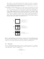
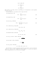
Katholieke Universiteit Leuven Departement Elektrotechniek Afdeling ESAT/MI2 Laboratorium voor Medische Beeldvorming (ESAT-Radiologie) Kardinaal Mercierlaan 94 B-3001 Heverlee - Belgium TECHNISCH RAPPORT - TECHNICAL REPORT Multimodality Image Registration using Information Theory (MIRIT), Version 97/08 Manual Pages Frederik Maes, Dirk Vandermeulen and Paul Suetens September 1997 Nr. KUL/ESAT/MI2/9708 Multimodality Image Registration using Information Theory M.I.R.I.T. Version 97/08 Manual Pages Frederik Maes1 , Dirk Vandermeulen, Paul Suetens. Katholieke Universiteit Leuven Medical Image Computing (ESAT-Radiology) UZ Gasthuisberg, Herestraat 49, B-3000 Leuven, Belgium E-mail: [email protected] 1 Frederik Maes is Aspirant of the Fund for Scientific Research - Flanders (Belgium). Abstract This document describes the MIRIT software developed at the Laboratory for Medical Imaging Research of the K.U.Leuven for automated affine registration of multimodal medical images. MIRIT implements the registration algorithm described in [1]. The method is based on maximization of the mutual information between corresponding voxel intensities in the two images to be registered. Because no limiting assumptions are made regarding the image content and the nature of the relation between corresponding voxel intensities, this criterion is very general and powerful, allowing for completely automated and robust registration in a variety of applications without prior segmentation or other preprocessing. The accuracy of the method has been validated to be subvoxel [1, 2] for rigid body registration of CT, MR and PET brain images compared to the stereotactic reference registration solution. MIRIT also allows to compute one-dimensional traces of the registration criterion through registration space and to reformat the images at the registered position. The MIRIT software and this manual is distributed without warranty and the software is to be used for experimentation only. All questions or feedback relating to this software or requests to obtain the MIRIT software should be addressed to Frederik Maes at the address mentioned above. This document has two parts. Part one describes some implementation specifics of the program, the second part describes how to install and use it. Part I Implementation issues 1 Chapter 1 The geometrical transformation 1.1 Coordinate frames and axis orientation With each of the images to be registered is associated an image coordinate frame in voxel units with its origin in the first voxel of the image, the x-coordinate corresponding to the column number, the y-coordinate to the row number and the z-coordinate to the slice number, assuming that the data are stored row by row and slice by slice (row major order). With each of the images is also associated a world coordinate frame in millimeter units with its origin positioned in the center of the image volume, defined in image coordinates by c = (cx , cy , cz ) = (d − 1)/2, with d = (dx , dy , dz ) being the dimensions of the image in directions x, y and z respectively. The axes of the world coordinate frame are defined with respect to the patient, the x-axis running from patient’s right to patient’s left (R/L), the y-axis from patients’s anterior to patient’s posterior (A/P) and the z-axis from patient’s inferior to patient’s superior (I/S). The orientation of each of the image coordinate axes (column, row and slice direction) with respect to the world or patient coordinate frame has to be specified for each of the images. This allows to compute image-to-image transformations of for instance transversal CT images to sagittal MR images. Each axis can have 6 possible orientations as defined in table 1.1. The image orientation o = (ox , oy , oz ) is specified by 3 numbers with values 1, -1, 2, -2, 3 or -3. The default orientations (on Siemens scanners) for CT and axial, sagittal and coronal MR images are depicted in figure 1.1. Orientation 1 -1 2 -2 3 -3 From patient’s right left anterior posterior inferior superior to patient’s left right posterior anterior superior inferior Table 1.1: Definition of image axis orientations. 1.2 The image-to-world transformation The transformation of homogeneous image coordinates p to homogeneous world coordinates w is defined by the center c of the image in image coordinates, its voxelsizes v = (vx , vy , vz ) in millimeter and the orientation o of the image axes w.r.t. the world coordinate frame: w = (O ∗ V ∗ C). p 2 CT Origin = RAI o = (1, 2, 3) 1 0 0 0 1 0 O= 0 0 1 0 0 0 Axial MR Origin = RAS o = (1, 2, −3) 1 0 0 0 1 0 O= 0 0 −1 0 0 0 0 0 0 1 Sagittal MR Origin = RAS o = (2, −3, 1) 0 0 1 0 O= 0 −1 0 0 1 0 0 0 0 0 0 1 Coronal MR Origin = RPS o = (1, −3, −2) 1 0 0 0 O= 0 −1 0 0 0 −1 0 0 0 0 0 1 0 0 0 1 Figure 1.1: Standard orientation of image coordinate frames for different modalities. 3 with C, V and O 4 × 4 transformation matrices that represent translation of the origin to the image center c, scaling by the voxelsizes v and permutation of the axes according to o respectively: 1 0 0 −cx 0 1 0 −cy C= 0 0 1 −cz 0 0 0 1 vx 0 0 0 0 vy 0 0 V = 0 0 vz 0 0 0 0 1 and O = {Oij } is given by (see figure 1.1) sign(oj ) if i = abs(oj ) − 1 Oij = 0 otherwise Eventually, for CT images, a non-zero gantry tilt can also be taken into account: w = (O ∗ Γ ∗ V ∗ C). p with Γ defined by the gantry tilt γ (measured in radians) by 1 0 0 0 cos(γ) 0 Γ= 0 sin(γ) 1 0 0 0 0 0 0 1 assuming that γ is positive for rotation of the top of the gantry caudally from patient’s head towards patient’s feet (as is the case on Siemens scanners). The image-to-world transformation matrix Ti,w is thus given by w = Ti,w . p Ti,w 1.3 Ti,w = O ∗ Γ ∗ V ∗ C 0 0 −vx .cx vx 0 cos(γ).vy 0 −vy .cy =O∗ 0 sin(γ).vy vz −vz .cz 0 0 0 1 (1.1) The affine world-to-world transformation The affine transformation that transforms world coordinates w 1 in image 1 into world coordinates w 2 in image 2 is defined by the 4 × 4 matrix A w 2 = A.w 1 with A of the form A=T ∗R∗G∗S (1.2) with S, G, R and T being 4×4 matrices respresenting scaling, skew, rotation, and translation respectively. The affine transformation is defined by 12 parameters α : 3 translation distances ti , 3 rotation angles φi , 3 skew factors gi and 3 scale factors si , from which the matrices T , R, G and S are computed as described below. Alternative definitions of A are possible, such as for instance A = T ∗ G ∗ S ∗ R, but definition 1.2 has the advantage that S can be interpreted directly as correction factors to be applied to the voxelsizes of image 1, such that S ∗ V represents the correctly calibrated voxelsizes of this image. This interpretation 4 is important when the voxelsizes of image 1 are not precisely known. Moreover, if image 1 is a CT-image with orientation [1, 2, 3] for which a gantry tilt was applied when acquiring image 1, the gantry angle γ can be recovered from G ∗ S as γ = atan(gz ). The translation matrix T is defined by the 3 translation parameters tx , ty and tz (expressed in millimeter) representing translation along the x, y and z axis respectively: 1 0 0 tx 0 1 0 ty T = (1.3) 0 0 1 tz 0 0 0 1 The rotation matrix R is the product of 3 matrices Rx , Ry and Rz defined by the 3 rotation parameters φx , φy , and φz (expressed in radians), representing rotation around the x, y and z axis respectively: R = Rx ∗ Ry ∗ Rz 1 0 0 0 cos(φx ) sin(φx ) Rx = 0 − sin(φx ) cos(φx ) 0 0 0 cos(φy ) 0 − sin(φy ) 0 1 0 Ry = sin(φy ) 0 cos(φy ) 0 0 0 cos(φz ) sin(φz ) 0 − sin(φz ) cos(φz ) 0 Rz = 0 0 1 0 0 0 0 0 0 1 0 0 0 1 0 0 0 1 such that R is given by (denoting cos(φi ) and sin(φi ) by cosi and sini respectively) cosy . cosz cosy . sinz − siny sinx . siny . cosz − cosx . sinz sinx . siny . sinz + cosx . cosz sinx . cosy R= cosx . siny . cosz + sinx . sinz cosx . siny . sinz − sinx . cosz cosx . cosy 0 0 0 0 0 0 1 (1.4) The skew matrix G is the product of 3 matrices Gx , Gy and Gz defined by the 3 skew parameters gx , gy and gz , representing skew in the x, y and z direction respectively: G = Gx ∗ Gy ∗ Gz 1 0 gx 0 0 1 0 0 Gx = 0 0 1 0 0 0 0 1 1 0 0 0 gy 1 0 0 Gy = 0 0 1 0 0 0 0 1 1 0 0 0 0 1 0 0 Gz = 0 gz 1 0 0 0 0 1 5 such that G is given by 1 gy G= 0 0 gx .gz 1 gz 0 gx 0 1 0 The scale matrix S is defined by the 3 scale parameters x, y and z axis respectively: sx 0 0 0 sy 0 S= 0 0 sz 0 0 0 0 0 0 1 (1.5) sx , sy and sz , representing scaling along the 0 0 0 1 (1.6) The overall expression for A = {Aij } as function of the affine transformation parameters α = {ti , φi , gi , si } is given by: A00 = sx .(cosy . cosz +gy . cosy . sinz ) A01 = sy .(cosy . sinz −gz . siny +gx .gz . cosy . cosz ) A02 = sz .(gx . cosy . cosz − siny ) A03 = tx A10 = sx .((sinx . siny . cosz − cosx . sinz ) + gy .(sinx . siny . sinz + cosx . cosz )) A11 = sy .((sinx . siny . sinz + cosx . cosz ) + gz . sinx . cosy +gx .gz .(sinx . siny . cosz − cosx . sinz )) A12 = sz .(sinx . cosy +gx .(sinx . siny . cosz − cosx . sinz )) A13 = ty A20 = sx .((cosx . siny . cosz + sinx . sinz ) + gy .(cosx . siny . sinz − sinx . cosz )) A21 = sy .((cosx . siny . sinz − sinx . cosz ) + gz . cosx . cosy +gx .gz (cosx . siny . cosz + sinx . sinz )) A22 = sz .(cosx . cosy +gx .(cosx . siny . cosz + sinx . sinz )) A23 = tz A30 = 0 A31 = 0 A32 = 0 A33 = 1 1.4 The image-to-image transformation The affine geometrical transformation of image coordinates p1 (measured in voxels) in image 1 into image coordinates p2 in image 2 is defined by w 2 = A.w 1 Ti,w,2 . p2 = A.(Ti,w,1 . p1 ) −1 ∗ A ∗ Ti,w,1 ). p1 p2 = (Ti,w,2 p2 = T12 . p1 (1.7) with Ti,w,1 and Ti,w,2 being the image-to-world coordinate transformation matrices for images 1 and 2 respectively, A the affine world-to-world transformation matrix mapping world coordinates in image 1 into world coordinates in image 2 and T12 the affine image-to-image transformation matrix mapping image coordinates in image 1 into image coordinates in image 2. T12 is thus given by −1 T12 = Ti,w,2 ∗ A ∗ Ti,w,1 (1.8) T12 incorporates the differences in orientation, resolution and relative position of the images 1 and 2. 6 1.5 Implementation of the image-to-image transformation One of the images to be registered is selected as the floating image from which samples are taken and transformed into the volume of the other image, the reference image. The image-to-image transformation is computed from the floating image into the reference image. The image-to-world coordinate transformation matrices Ti,w,1 and Ti,w,2 are constructed for both the floating and the reference image respectively using expression 1.1. These matrices are independent of the actual geometrical transformation between both images and are fixed given the image dimensions, voxel sizes and axes orientation. For a given set of affine registration parameters α = (tx , ty , tz , φx , φy , φz , gx , gy , gz , sx , sy , sz ) the matrices S, G, R, T and A are constructed using expressions 1.6, 1.5, 1.4, 1.3 and 1.2. The image-toimage transformation matrix T12 is computed using expression 1.8. The transformation of all points p1 in the floating image into points p2 in the reference image using expression 1.7 can be efficiently evaluated using addition operations only. Indeed, because of the linearity of the transformation, the columns of matrix T12 represent the transformed position p2,o of the origin p2 in position in image 2 for differential changes p1,o of image 1 in image 2 and the differential changes ∆ ∆ p2 in position in image 1: p1,o = [0 0 0 1] p2,o = T12 . p1,o = T12 (:, 4) p2,o + ∆ p2 = T12 .( p1,o + ∆ p1 ) p1 ∆ p2 = T12 .∆ ∆x p1 = [1 0 0 1] ⇒ ∆x p2 = T12 (:, 1) p1 = [0 1 0 1] ⇒ ∆y p2 = T12 (:, 2) ∆y ∆z p1 = [0 0 1 1] ⇒ ∆z p2 = T12 (:, 3) p1,o = T12 (:, 4) of the origin of the floating image into the Given the transformation p2,o = T12 . reference image, the transformed position p2 of all other points p1 of the floating image is computed incrementally while scanning the floating image and incrementing p2 with T12 (:, 1), T12 (:, 2) or T12 (:, 3) for a step in the floating image along the x, y or z image axis respectively. 1.6 Computing the parameters of the affine transformation Given the 12 affine transformation parameters α = {ti , φi , gi , si }, the affine transformation matrix A can be straightforwardly computed by the matrix multiplications described above. Here we are interested in the inverse problem: decomposing a given affine transformation matrix A into A = T ∗ R ∗ G ∗ S with T , R, G and S of the form defined above, i.e. computing α from A. This is useful if the transformation A of image 1 into image 2 is known and we wish to use the parameters of the inverse transformation A−1 to reformat image 1 along the grid of image 2. The translation parameters tx , ty , tz of the transformation are simply given by ti = Ai4 from which the translation matrix T can be constructed. Once T has been found, the scale and skew parameters can be most easily computed from L = T −1 ∗ A = R ∗ G ∗ S using the fact that the rotation matrix R is orthonormal: RT = R−1 . The product P of L and its transpose LT is therefore independent of R: L = T −1 ∗ A = R ∗ G ∗ S P = = LT ∗ L (R ∗ G ∗ S)T ∗ (R ∗ G ∗ S) = = S T ∗ GT ∗ RT ∗ R ∗ G ∗ S S ∗ GT ∗ G ∗ S 7 The 6 skew and scale parameters can be computed from P by solving for gi and si the set of 6 non-linear equations S ∗ GT ∗ G ∗ S = P with s2x .(1 + gy2 ) sx .sy .(gy + gx .gz ) S ∗ GT ∗ G ∗ S = sx .sz .gx 0 sx .sy .(gy + gx .gz ) s2y .(1 + gz2 .(1 + gx2 )) sy .sz .gz .(1 + gx2 ) 0 sx .sz .gx sy .sz .gz .(1 + gx2 ) s2z .(1 + gx2 ) 0 0 0 0 1 using the additional relation that sx .sy .sz = det(L) Solving these equations yields the following expressions for gi and si , with D = det(L): s2y = s2x = s2z = 2 P12 P22 (P01 .P22 − P02 .P12 )2 P00 − 2 .s2 P22 y P11 − g̃x = g̃y = g̃z = sx = P2 P22 − 02 s2x s2 x s2y s2z |sy | P02 . D P01 .P22 − P02 .P12 |sz | . P22 D 2 P12 sz .|sx | . P22 D sign(sx ).|sx | sy = sign(sy ).|sy | sz gx = = sign(sz ).|sz | sign(sy ).g̃x gy gz = = sign(sz ).g̃y sign(sx ).g̃z |sx | = |sy | = |sz | = in which the sign of the scale factors has yet to be determined. From the computed ti , si and gi , the matrices T , S and G can be reconstructed and the rotation matrix R can be derived as R = T −1 ∗ A ∗ (G ∗ S)−1 = L ∗ S −1 ∗ G−1 using expressions 1.6 and 1.5 for S −1 and G−1 . The sign of the scale factors can be determined such that the elements R00 = cos(φy ). cos(φz ) and R22 = cos(φx ). cos(φy ) of R are positive. All rotation parameters φi can then be assumed to be in the range [−π/2, π/2]. These conditions can be expressed as R00 = R22 = − 1 gy gy .gz .L00 − .L01 + .L02 ≥ 0 sx sy sz gx gx .gy 1 − gx .gy .gz .L20 + .L21 + .L22 ≥ 0 sx sy sz 8 Substituting the expressions for gi , these conditions are equivalent to sign(sx ).( sign(sz ).(− 1 g̃y g˜y .g˜z .L00 − .L01 + .L02 ) ≥ 0 |sx | |sy | |sz | g̃x g̃x .g̃y 1 − g̃x .g̃y .g̃z .L20 + .L21 + .L22 ) ≥ 0 |sx | |sy | |sz | from which the appropriate signs can be derived to be sign(sx ) = sign(S1 ) sign(sy ) sign(sz ) = sign(S1 ).sign(S2).sign(D) = sign(S2 ) with S1 = S2 = − 1 g̃y g˜y .g˜z .L00 − .L01 + .L02 |sx | |sy | |sz | g̃x g̃x .g̃y 1 − g̃x .g̃y .g̃z .L20 + .L21 + .L22 |sx | |sy | |sz | The sign(S1 ).sign(S2).sign(D) factor in the expression for sy assures that sx .sy .sz has the same sign as D. Finally, the rotation parameters φi can be derived from R: φy φx φz = −asin(R02 ) R12 ) = asin( cos(φy ) R01 ) = asin( cos(φy ) 9 Chapter 2 The registration measure 2.1 Histogram computation The mutual information of the images to be registered at the current registration position α is evaluated from the joint histogram of the image intensities of the overlapping volume of the images at this position. Let SF = { pF } be the set of samples pF taken from the floating image F and transformed by the α) into the set SR = { pR = T12 ( α). pF } in the reference image R. image-to-image transformation T12 ( Only those samples pF ∈ SF,α ⊂ SF are retained for which pR falls inside the volume of R. pR ) denote the image intensity values in image F at position pF and in image R at Let f ( pF ) and r( the transformed position pR respectively. The joint image intensity histogram Hα (f, r) of the overlapping part of F and R is computed by binning the image intensity pairs (f ( pF ), r( pR )) for all pF ∈ SF,α . The number of bins nF and nR to be used for the floating and reference image intensities respectively are parameters to be specified by the user. Typically, we use nF = nR = 256. In order to do the binning efficiently, the floating and the reference image intensities are first linearly rescaled between [1, nF − 1] and [1, nR − 1] respectively. The histogram bins {H(0, r), r = 0, 1, . . . , nR − 1} and {H(f, 0), f = 0, 1, . . . , nF − 1} are not being considered when computing the mutual information criterion. This allows to use the value 0 in either image for special purposes, such as to mark regions in the image that one wants to exclude when computing the registration measure. A rectangular region of interest and sampling factors along each axis separately can be specified in either image. The original images are first resampled using trilinear interpolation within these regions. Only the voxels inside the overlapping volume of these regions are considered when computing the joint image intensity histogram and the registration criterion. Subsampling the floating image aims at increasing speed performance (see also section 3.3), while supersampling the floating or the reference image aims at increasing registration precision. 2.2 Interpolation While all samples pF are taken at grid points of the floating image F, their transformed positions pR will in general not coincide with a grid point of the reference image R and interpolation of the reference image is needed to obtain the image intensity value r( pR ) at this position. Three interpolation methods have been implemented (see figure 2.1): Nearest neighbour (NN) interpolation The nearest neighbour of pR on the grid of R is found. If this neighbour is inside the volume of R, its intensity value is assigned to r( pR ) and the histogram is updated by adding 1 to the entry corresponding to (f ( pF ), r( pR )). Nearest neighbour interpolation is generally insufficient to guarantee subvoxel accuracy, as it is insensitive to translations up to one voxel. Trilinear (TRI) interpolation The 8 nearest neighbours of pR on the grid of R are found. If all these neighbours are inside the volume of R, their intensities are linearly interpolated and this 10 value is assigned to r( pR ). The histogram is updated by adding 1 to the entry corresponding to (f ( pF ), r( pR )). Linear interpolation may introduce new intensity values which are originally not present in the image R, leading to unpredictable changes in the marginal histogram of the reference image for small changes in the registration parameters. Partial volume (PV) interpolation The 8 nearest neighours of pR on the grid of R are found. For all neighbours ni , i = 1, 2, . . . , 8 that fall inside the volume of R, the histogram is updated by adding p1 ), r(ni )), wi being the linear interpolation weight associated with neighbour i wi to entry (f ( (0 ≤ wi ≤ 1). To avoid having to test for each neighbour separately whether it falls inside the volume of R, R is expanded into Rb by appending a one-voxel wide border to the reference volume at all sides, which is assigned the value zero. The histogram is updated for each sample for which pR falls inside the volume of Rb . Because histogram entries with reference image zero are not taken into account when computing the registration criterion, only those neighbours that fall inside the volume of R are effectively being considered. Because the histogram is build up as the sum of , the histogram and thus the fractions wi that vary smoothly with the registration parameters α mutual information measure itself is a continuous function of α . n4 r rn3 ✚ ❃ ✚ ✚ s p R NN: n1 r n2 rn3 w2 s TRI: w3 w1 p R w4 r( pR ) = r i wi ( pR ) = 1 i wi . r(ni ) Hα pF ), r( pR )) += 1 (f ( r n2 n4 r rn3 w2 PV: w3 n1 r( pR ) = r(n3 ) pF ), r( pR )) += 1 Hα (f ( r n4 r n1 arg minni d( p R , ni ) = n3 s w1 p R w4 r i wi ( pR ) = 1 ∀i : Hα pF ), r(ni )) += wi (f ( r n2 Figure 2.1: Graphical illustration of NN, TRI and PV interpolation in 2-D. NN and TRI interpolation find the reference image intensity value at position pR and update the corresponding joint histogram entry, while PV interpolation distributes the contribution of this sample over multiple histogram entries defined by its nearest neighbour intensities, using the same weights as for TRI interpolation. 2.3 Criterion Once the joint image intensity histogram Hα (f, r) has been constructed as described above, estimations for the joint and marginal probability density functions of the image intensities in the overlapping volume of images F and R are obtained by normalization of H: N= n F −1 n R −1 f =1 r=1 11 Hα (f, r) p(f, r) = Hα (f, r)/N n R −1 p(f ) = p(f, r) r=1 p(r) = n F −1 p(f, r) f =1 Histogram bins corresponding to value zero in either image are not being taken into account as explained in sections 2.1 and 2.2. Various information theoretic measures are then computed as follows: • the marginal entropy of F: HF = − n F −1 p(f ). log2 p(f ) (2.1) p(r). log2 p(r) (2.2) f =1 • the marginal entropy of R: HR = − n R −1 r=1 • the joint entropy of F and R: HF R = − n F −1 n R −1 f =1 p(f, r). log2 p(f, r) (2.3) r=1 • the conditional entropy of F given R: HF |R = HF R − HR • the conditional entropy of R given F: HR|F = HF R − HF • the mutual information of F and R: IF R = HF + HR − HF R (2.4) • the entropy correlation coefficient of F and R: 'F R = 2. IF R HF + H R • the uncertainty coefficient of F and R: UF R = IF R HR • the entropy metric of F and R: ρF R = HF |R + HR|F = HF R − IF R HF , HR and HF R are computed from the histogram H using expressions 2.1, 2.2 and 2.3 and all other quantities are computed from these. MIRIT allows all these quantities to be specified as the registration criterion, although only IF R , 'F R , UF R and ρF R are meaningful. 12 Chapter 3 Search The optimal set of registration parameters α ∗ is defined as α ∗ = arg max I( α) α (3.1) with I the mutual information of the intensities of corresponding voxels in both images to be registered (or any other criterion specified in MIRIT). The optimization method that is used for registration is a straightforward implementation of the Powell direction set method as discussed in [3], chapter 10, pp. 412-420. For the line minimizations, the Brent algorithm is used (see [3], chapter 10, pp. 402-405). Because the measures IF R , 'F R and UF R need to be maximized while the implementation of the Powell algorithm allows minimization only, these measures are internally converted into measures that are minimal when the original measures are maximal. The conversions used are: Iˆ = log2 (min(nF , nR )) − I 'ˆ = 1 − ' Û = 1 − U with nF and nR the number of histogram bins used for the floating and the reference image respectively. Because 0 ≤ I ≤ log2 (min(nF , nR )), 0 ≤ ' ≤ 1 and 0 ≤ U ≤ 1, these measures obey 0 ≤ Iˆ ≤ log2 (min(nF , nR )), 0 ≤ 'ˆ ≤ 1 and 0 ≤ Û ≤ 1. 3.1 The line minimization algorithm The implementation of the line minimization algorithm is based on the routines linmin, mnbrak and brent in [3], chapter 10. The parameters that determine convergence and that have to be specified by the user are: • the initial step taken when bracketing the minimum (i.e. 1.0 in the routine linmin in [3], pp. 419). This is a parameter to be specified by the user, as for instance a step of 1.0 has a different impact for scaling and skew than for translation and rotation. Default values are 1.0 mm for translation, 1.0 degree for rotation and 0.1 for scaling and skew. These initial step values are decreased by a factor of 2 after each Powell iteration in order to try to minimize the number of evaluations required for the line minimization as the optimization nears the optimum. • the maximal step taken when bracketing the minimum (i.e. GLIMIT in the routine mnbrak in [3], pp. 400-401). Default value is 10 for all directions. • the fractional precision to which the minimum is isolated (i.e. tol in the routine brent in [3], pp. 404-405). Default value is 10−3 for all directions. 13 • the absolute precision to which the minimum is isolated. This parameter is not included in the routine brent in [3], pp. 404-405. It is included here to declare convergence when the bracket is smaller than, say, 0.01 mm or 0.1 degrees. Default value is 10−4 for all directions. • the maximum allowed number of iterations (i.e. ITMAX in the routine brent in [3], pp. 404-405). Default value is 20. 3.2 The Powell algorithm The implementation of the Powell algorithm is based on the routine powell in [3], chapter 10, pp. 417-418. The parameters that determine convergence and that have to be specified by the user are: • the order in which the parameters are optimized. The direction matrix is initialized with unit vectors in each direction. The order in which these directions are considered may greatly influence optimization robustness, due to the fact that the image resolution is generally not the same along all axes. • the maximum allowed number of iterations (i.e. ITMAX in the routine powell in [3], pp. 417-418). Default value is 20. • the fractional tolerance in the function value (i.e. ftol in the routine powell in [3], pp. 417-418). Default value is 10−5 . • a flag indicating whether or not the direction matrix should be updated when a new direction has been determined. New directions are considered according to the criteria discussed in [3], pp. 416-417. Default behavior is not to update the direction matrix. 3.3 Multiresolution optimization Because the time required to evaluate the registration criterion is proportional to the number of samples taken from the floating image and transformed into the reference image to construct the joint image intensity histogram, large speedups are possible by starting the optimization at a lower resolution by subsampling the floating image and by switching to a higher resolution by including more samples as the optimization proceeds. A straightforward multiresolution strategy has been incorporated in MIRIT. The number of resolution levels and the resolution factor from one level to the next has to be specified for each axis of the floating image. The floating image is simply subsampled without prior lowpass filtering in order not to introduce new intensity values in the subsampled images. The optimization is started using the subsampled image at the lowest resolution level and the method switches to the next resolution level when convergence is reached at the previous level. Experiments have indicated that the robustness of the method is not affected by subsampling the floating image as long as moderate subsampling factors (2 to 4 along each axis) are used, depending on the resolution of the original floating image. Using more than 2 resolution levels (a lower resolution one and the full resolution level) results generally in slower overall convergence, due to the additional evaluations that are needed to reach convergence at the intermediate resolution level. When more than 1 resolution level is specified, the speed performance can usually be increased by limiting the number of Powell iterations at each level, for instance by setting the maximum allowed number of Powell iterations to 5 (instead of 20 by default). 14 Part II User’s manual 15 Chapter 4 Running the program 4.1 Platforms The Mirit software was developed in C++ on an IBM RS6000 workstation under AIX 4.1.3 using IBM’s xlC compiler and has been ported to SUN, HP and SGI using the CC compiler. Porting to other platforms, such as PC, should not pose too many problems, due to the fact that the code is completely self-contained, does not require external libraries except for the standard C++ library and does not use the template class mechanism. 4.2 Installation The program is distributed as a compressed tar-file Mirit.tar.gz. First move this file to the directory in which the program has to be installed, keeping in mind that extracting the code from this file will itself create a subdirectory Mirit. The code can be extracted from this file by > gunzip Mirit.tar.gz > tar -xvf Mirit.tar This will create the following directory structure: ./Mirit/include/MIChrono.h MIImageGrid.h MIManager.h MIMeasure.h MIOptimisation.h MIParams.h MIPrint.h MIReformat.h MIShrtImage.h MITrace.h MITransform.h MITypes.h ./Mirit/src/MIChrono.C MIImageGrid.C MIManager.C MIMeasure.C MIMirit.C MIOptimisation.C MIParams.C MIReformat.C MIShrtImage.C 16 MITrace.C MITransform.C MakefileHP MakefileIBM MakefileIBMPW2 MakefileSGI MakefileSUN ./Mirit/bin ./Mirit/lib ./Mirit/man/MiritManual.ps.gz (= this document) ./Mirit/examples/MIRITinput MIRITimages MIRITparams 4.3 Compilation The program can be compiled by running (depending on your platform) > make -f MakefileIBM (xlC compiler) or > make -f MakefileIBMPW2 (xlC compiler for IBM Power 2 architecture) or > make -f MakefileSUN (CC compiler) or > make -f MakefileHP (CC compiler) or > make -f MakefileSGI (CC compiler) in the ./Mirit/src directory. This creates the library ./Mirit/lib/libMiritX.a and the executable ./Mirit/bin/MiritX, with X the architecture name (IBM, IBMPW2, SUN, HP or SGI). The compiler flags have been set to generate optimized code (-O3) for each platform. For SGI, some flags (-ip) have to be adapted to match the processor type. See the manual pages for CC on your platform. 4.4 Starting the program The MIRIT program has no fancy user interface, but is designed to run off-line, reading its input from a number of input files and writing its output to an output file. Assuming that the program executable Mirit resides in the directory /home/registration/Mirit/bin, the program can be run from the working directory /home/registration/Mirit/experiment by the commands > cd /home/registration/Mirit/experiment > /home/registration/Mirit/bin/Mirit MIRITinput The file MIRITinput (which should be in the working directory) specifies all input to the program. All input filenames mentioned in this document are arbitrary. Examples of the MIRIT input files can be found in the ./Mirit/examples directory. The format of the MIRITinput file is discussed in chapter 5. 17 Chapter 5 Passing input to the program 5.1 Specifying the operation mode: MIRITinput The file MIRITinput specifies the image data, the user controllable parameters, the mode in which the program should operate and the name of the file in which the program writes its output. It has the following contents: MIRITimages MIRITparams 1 MIRIToutput.m < < < < filename filename number filename : : : : image data > parameters > operation mode : 1, 2, 3 or 4 > output file > MIRITimages MIRITimages is the name of the file that specifies the floating and reference image data. The format of this file is discussed in section 5.2. This file should be accessible from the working directory from which the program is started. MIRITparams MIRITparams is the name of the file that specifies all user controllable parameters. The format of this file is discussed in section 5.3. This file should be accessible from the working directory from which the program is started. MIRIToutput MIRIToutput is the name of the file to which the program writes its output. The output format depends on the operation mode in which the program runs. For registration, the outputfile is in Matlab [4] format. If a directory path is specified (dirpath filename) this should be accessible from the working directory. If no directory path is specified, the file is written in the working directory. Operation mode The operation mode defines the behaviour of the program. Currently, the following modes are defined: • 1 = registration : computes the optimal registration position of the images specified by MIRITimages using the registration parameters specified by MIRITparams and writing the registration results to file MIRIToutput • 2 = tracing : computes a trace of the registration criterion through parameter space for the images specified by MIRITimages using the trace parameters specified by MIRITparams and writing the trace values to file MIRIToutput • 3 = histogram : computes the joint intensity histogram of the images specified by MIRITimages at their relative position specified by MIRITparams and writing the histogram image to file MIRIToutput 18 • 4 = reformatting : reformats the reference image specified by MIRITimages along the grid of the floating image at the relative position of the images specified by MIRITparams and writing the reformatted image to file MIRIToutput If any other number is specified, the program exits. 5.2 Image data specification : MIRITimages The program reads the images from user specified files, assuming that the image data are stored contiguously row by row and slice by slice using 16 bits per voxel (short). The image data file may have a header and the user can specify the number of bytes to skip from the beginning of the file. The dimensions and voxelsizes of the images have to be specified in the file MIRITimages. This file has the following contents: 2 1 2 3 256 256 180 0.9765625 0.9765625 1.0 0.0 /images/registration/MR.img 512 0 255 0 255 0 179 1.0 1.0 1.0 1 2 3 256 256 100 0.9375 0.9375 1.55 0.0 /images/registration/CT.img 512 0 255 0 255 0 99 1.0 1.0 1.0 < < < < < < < < < < < < < < < < < number of images to be registered > reference image orientation > reference image dimensions > reference image voxel sizes > reference image gantry > reference image file name > reference image file header > reference image ROI > reference image sampling factors > floating image orientation > floating image dimensions > floating image voxel sizes > floating image gantry > floating image file name > floating image file header > floating image ROI > floating image sampling factors > The number of images specified should always be 2. The first image specified is taken to be the reference image, the second image specified is the floating image. Samples are taken from the floating image and transformed into the reference image to compute the joint image intensity histogram of the overlapping volume of both images. The speed of the method is increased by selecting the smaller image of the two to be the floating image. Each of the images is specified by the following parameters in this order: Dimensions along the x (column), y (row) and z (slice) axis respectively Orientation of the x, y and z axis respectively as defined in section 1.1 Voxel sizes in mm along the x (column), y (row) and z (slice) axis respectively Gantry tilt in degrees. This is the angle between the imaging plane and the plane orthogonal to the slice axis for CT images. The gantry tilt is assumed to be positive if the top of the gantry is tilted towards the patient’s feet (caudally) and is negative if the top of the gantry is tilted towards the patient’s head (cranially). This number should always be 0.0 for MR and PET images. File name including directory path and Header length in bytes. The image data are read from the specified file name, skipping the specified number of bytes for the file header. MIRIT requires that the image data are stored contiguously row by row and slice by slice using 16 bits (short) per voxel. The program exits if the specified file can not be opened or if the number of voxels read from file does not match the specified dimensions. 19 Region of interest The program allows for a rectangular region of interest (ROI) to be defined in either image. Only voxels inside this ROI will be taken into account when computing the registration criterion. The ROI is specified by the first and last image coordinates [xmin xmax ymin ymax zmin zmax ] of the region along each of the axes. These coordinates have to be specified even if the full image is to be considered. Sampling The program allows to first resample either image within the specified ROI before registration. This allows to artificially increase the resolution of the reference image for higher precision or to decrease the resolution of the floating image to increase speed performance. Sampling of the images is specified by the sampling factors [fx fy fz ] along each dimension. A sampling factor of fx for the x dimension means that 1 out of every fx voxels along the image row axis is sampled. Sampling is done using trilinear interpolation. Each image can be either supersampled (f < 1) or subsampled (f > 1) within the specified ROI. Sampling factors of 1.0 in each dimension have to be specified if no sub- or supersampling has to be applied. 5.3 Parameter specification : MIRITparams All user controllable parameters are specified in the file MIRITparams. Their interpretation may depend on the operation mode of the program (registration, tracing, histogram or reformatting). All parameters have to be specified in all cases, although some parameters are not used in some operation modes. The contents of the parameter file MIRITparams are : 0.0 0.0 0.0 0.0 0.0 0.0 1.0 1.0 1.0 0.0 0.0 0.0 5 6 3 1 2 4 0 0 0 0 0 0 10 1.0 0.0 0.0 0.0 0.0 0.0 0.0 0.0 0.0 0.0 0.0 0.0 4 256 256 3 2 2 2 3 3 2 1 10.0 1e-4 1e-3 20 1e-5 20 0 < < < < < initial position > parameter order > nr of steps, step sizes > criterion parameters > optimization parameters > Initial position The initial position specifies the initial value for each of the 12 registration parameters in the order φx , φy , φz , tx , ty , tz , sx , sy , sz , gx , gy , gz (φ being the rotation parameters, t the translation parameters, s the scaling factors and g the skew parameters). Rotation parameters are specified in degrees, translation parameters in millimeter. In the example file above, the rotation, translation and skew parameters are initialized with 0.0, while the scaling factors are set to 1.0. These values are used in each of the operation modes. In registration mode, the optimization will be started from this initial position. In histogram and reformatting mode, the images are considered to be at this position. In tracing mode, the trace is computed with its center point corresponding to this initial position. Parameter order The next line specifies the order in which the parameters will be optimized over in the Powell algorithm. These values are only used in registration mode. In the example above, tx is optimized first, followed by ty , φz , φx and φy and finally tz . An entry of 0 means that the corresponding parameter will not be optimied over, but will be kept constant and equal to its initial value. In the example above, the three scaling parameters and the three skewing parameters are unaffected by the optimization and the affine transformation is restricted to a rigid body transformation only. The number of non-zero entries determines the number of directions in Powell’s direction set method. Different non-zero entries should start at 1 and be numbered consecutively. Registration parameters may be coupled and optimized together by assigning them the same order number. For instance, the parameter order specification 5 6 3 1 2 4 7 7 8 0 0 0 will force the scaling parameters in the x and y direction to vary simultaneously, such that if they had the same value initially, they will have the same value after optimization. Experiments have indicated that robustness is increased by first optimizaing the in-plane parameters (i.e. tx , ty and φz for an axial image) before optimizing the out-of-plane parameters (tz , φx and φy ) and that the non-rigid parameters si and gi are best optimized after the rigid parameters ti and φi . A reasonable specification for the parameter order in most cases is therefore 5 6 3 1 2 4 0 0 0 0 0 0 for rigid-body registration and 5 6 3 1 2 4 7 8 9 10 11 12 for full affine registration. 20 Step size The first parameter on this line, the number of steps parameter, is used in tracing mode only, while the next 12 parameters, the step size parameters - one for each affine parameter in the same order as used to specify the initial position, are used both in tracing and registration mode. In registration mode, the step sizes determine the size of the first step in the bracketing phase of the line minimization routine (see section 3.1). Default bracketing step values are 1.0 for rotation and translation and 0.1 for scaling and skewing, and these are decreased during optimization. If the specified step size parameter is zero, the defualt value is used. If the specified step size parameter is non-zero, the initial bracketing step is set to the step size parameter if this is larger than 0.001 and smaller than 10.0, otherwise the default value is used. In tracing mode, the step size parameters define the direction of a one-dimensional line in parameter space. Values of the registration criterion are computed along this trace direction at intervals of a step size in each parameter. The trace is computed symmetrically around the initial position and has a total length of 2 times the number of steps plus 1. Criterion parameters These parameters specify the registration measure: 4 256 256 3 2 2 2 3 3 2 < < < < < < < < < < registration criterion > number of reference image histogram bins > number of floating image reference bins > type of interpolation in reference image > number of resolution levels for column dimension > number of resolution levels for row dimension > number of resolution levels for slice dimension > resolution factor for column dimension > resolution factor for row dimension > resolution factor for slice dimension > These are explained below: Registration criterion This parameter specifies the information measure that is computed from the joint image intensity histogram and used as the matching criterion. The parameter is to be specified as follows: 1 = H(F,R) = the joint entropy of both images 2 = H(F|R) = the conditional entropy of the floating image 3 = H(R|F) = the conditional entropy of the reference image 4 = I(F,R) = the mutual information of both images 5 = U(F,R) = the uncertainty coefficient of both images 6 = ECC(F,R) = the entropy correlation coefficient of both images 7 = rho(F,R) = the entropy metric of both images other: invalid The program exits if a non-valid number is specified. Histogram size The joint histogram of the overlapping part of both images is computed by binning all pairs of floating and reference image intensity values of geometrically corresponding voxels in both images. The number of bins to be used for either image is specified by these parameters. Typically, a value of 256 is used for all images. Interpolation The type of interpolation to be used to obtain image intensity values in the reference image is specified by: 1 = nearest neighbour 2 = trilinear 3 = partial volume other: invalid The program exits if a non-valid number is specified. 21 Multi-resolution parameters These parameters have only effect in registration mode. To increase speed performance, MIRIT incorporates a multiresolution strategy for registration (see section 3.3). When the optimization starts, the criterion is computed from a coarsely sampled floating image, while at the end, as the optimization convergences, the full floating image resolution is considered. The number of resolution levels to be considered during optimization and the subsampling factors applied from one level to another is specified by the user for each dimension of the floating image. If resolution levels [1 1 1] are specified, no additional resolution levels will be considered and the complete optimization is done at full resolution. If resolution levels [2 2 1] are specified together with resolution factors [2 2 2], 2 resolution levels will be used. The floating image is first subsampled by a factor of 2 along the column and row direction, but not along the slice direction. The optimization starts using this subsampled image, and proceeds with the full resolution image. If resolution levels [3 3 2] and resolution factors [2 2 2] are specified, 3 resolution levels will be used, with subsampling factors of [4 4 2], [2 2 2], and [1 1 1] respectively. In the example above, 2 resolution levels are used, one using subsampling factors [3 3 2] and the other at full floating image resolution. Optimization parameters These parameters are used in registration mode only. They specify the convergence parameters for the Powell algorithm and for the Brent line minimization routine. Referring to the example file above and the description of the optimization parameters in sections 3.1 and 3.2, the interpretation of the parameters is as follows: 1 10.0 1e-4 1e-3 20 1e-5 20 0 < < < < < < < < optimization method: should be 1 (= Powell) > Brent: maximum bracket step > Brent: absolute tolerance for convergence > Brent: relative tolerance for convergence > Brent: maximum number of iterations > Powell: relative tolerance for convergence > Powell: maximum number of iterations > Powell: update direction matrix if new direction is found > The values given here are the default values for these parameters. For most cases, it is not needed to change them. However, if more than one resolution level is used, the maximum number of Powell iterations is better set to 5 (instead of 20) to increase speed performance. 22 Chapter 6 Functionality When the program is started using > /home/registration/Mirit/bin/Mirit MIRITinput the files MIRITimages and MIRITparams as specified in MIRITinput are read and the images are loaded from file. The program mirrors its input on screen: MIRIT input file: MIRITinput MIRIT images file: MIRITimages MIRIT parameter file: MIRITparams MIRIT mode: 1 (registration) MIRIT output file: MIRIToutput.m LOADING IMAGES: Reference image: Orientation: [1 2 3] Dimensions: [256 256 180] Voxelsizes: [0.976562 0.976562 1.000000] Gantry: 0.000000 File: /images/registration/MR.img Header: 512 ROI: 0 255, 0 255, 0 179 Sampling: [1.000000 1.000000 1.000000] Floating image: Orientation: [1 2 3] Dimensions: [256 256 100] Voxelsizes: [0.937500 0.937500 1.550000] Gantry: 0.000000 File: /images/registration/CT.img Header: 512 bytes ROI: 0 255, 0 255, 0 99 Sampling: [1.000000 1.000000 1.000000] The program may run in one of 4 different operation modes, as specified by the operation mode parameter in the MIRITinput file described above. The functionality of each of these modes is described hereafter. 6.1 Registration mode The reference and the floating image are read from file as specified by the parameters in the file MIRITimages. The floating and reference images are resampled within the specified ROI. The world 23 coordinate frame for the cropped and resampled images is the same as the one assigned to the original images. Both the reference and the floating image intensities are rescaled linearly to the range [1,Nbins-1] with Nbins being the number of histogram bins as specified in the MIRITparams file for the reference and floating image respectively. The images are initially positioned according to the position parameters specified in the MIRITparams file, which are echoed to screen. Registration then involves optimizing the selected matching criterion. During optimization, the user can monitor the behaviour of the program from the output on the screen (figure 6.1). At each iteration, the criterion is optimized along a set of one-dimensional lines specified by Direction. These directions are initialized with unit vectors in each of the parameters seperately and are considered in the order as specified by the order parameters in MIRITparams as discussed above. Bracket and Brent denote the bracketing and Brent steps of the line minimization algorithm respectively. The initial guess for the bracket is determined by the step size paramaters in the MIRITparams file. The bracket values, the current guess for the optimum within this bracket and the corresponding function value are displayed at each step. Because some criteria needs to be minimized while others have to be maximized and because our implementation of the Powell algorithm only allows minimization, those criteria that require maximization are in fact converted to a related measure that is minimal when the true criterion is maximal. At the end of each line minimization step, the updated position is displayed, together with the number of evaluations so far. Convergence of each of the Brent steps and of the overall minimization process is determined by the convergence parameters specified in MIRITparams. The program terminates by writing the registration result to file which can be interpreted by Matlab [4] (provided it has been given the extension .m). The format of this output file is discussed in section 7. 6.2 Tracing mode The images are treated as in registration mode. Values of the registration measures are computed along a one-dimensional line in the parameter space and written to file which can be interpreted by Matlab [4] (provided it has been given the extension .m). The format of this output file is discussed in section 7. The position corresponding to the first value in the trace is determined from the number of steps and the initial position as specified in the MIRITparams file. The trace is computed symmetrically around this initial position, such that there are 2 times the number of steps plus 1 values in the trace and that the center value in the trace corresponds to the specified initial position. During program execution, the initial position and the current step along the trace are displayed, together with values for the number of floating image sample points in the overlapping volume (N), the joint entropy (H), the mutual information (I), and the entropy correlation coefficient (ECC), as well as the CPU time required to compute these values (figure 6.2). 6.3 Histogram mode In this mode, the joint histogram of the overlapping parts of both images is computed at the specified registration position and written to file. The input images are treated as in registration mode. The position for which the histogram is to be computed is defined by the registration parameters specified in the MIRITparams file. The histogram image data are stored contiguously using 8 bytes per entry (double). The number of columns in the histogram image equals the number of bins specified for the reference image, while the number of rows in the histogram image equals the number of bins specified for the floating image. The number of bins is specified in the MIRITparams file. A header of 128 bytes is added to the histogram output file describing the histogram image size (figure 6.4). 6.4 Reformatting mode In this mode, the reference image is reformatted along the grid of the transformed floating image. The reference and floating image are read from file, cropped and resampled according to the ROI and sam24 CRITERION PARAMETERS: Criterion: 4 ( I(X,Y) ) Reference image: 256 bins Floating image: 256 bins Interpolation: 3 (partial volume) Resolution levels: [2 2 2] , 2 levels Resolution steps: [3 3 2] OPTIMISATION PARAMETERS: Method: 1 (Powell) Line minimisation parameters: max bracket step: 1.00e+01 absolute tolerance: 1.00e-04 fractional tolerance: 1.00e-03 max iterations: 20 Convergence parameters: fractional tolerance: 1.00e-05 max iterations: 20 Powell parameters: order = [ 5 6 3 1 2 4 0 0 0 0 0 0 ]; steps = [ 1.00 1.00 1.00 1.00 1.00 1.00 0.10 0.10 0.10 0.10 0.10 0.10 ]; accept new direction: 0 REGISTRATION HAS STARTED ... Initial position: 0.0000000000 0.0000000000 0.0000000000 0.0000000000 0.0000000000 0.0000000000 1.0000000000 1.0000000000 1.0000000000 0.0000000000 0.0000000000 0.0000000000 Iteration 1, direction 1: 0.0000000000 0.0000000000 0.0000000000 1.0000000000 0.0000000000 0.0000000000 0.0000000000 0.0000000000 0.0000000000 0.0000000000 0.0000000000 0.0000000000 Bracket [ 0.0000000000 2.6180340000 ] 1.0000000000 7.421546973235 [ 2.6180340000 12.3911170327 ] 6.3510195276 7.403797011246 Brent [ 2.6180340000 8.6581314112 ] 6.3510195276 7.403797011246 [ 4.9251459775 8.6581314112 ] 6.3510195276 7.403797011246 ... Final position: 10.0683506925 -3.1541507013 2.0849665884 6.8953720978 1.1058616719 18.2236738732 1.0000000000 1.0000000000 1.0000000000 0.0000000000 0.0000000000 0.0000000000 OUTPUT TO FILE : MIRIToutput.m Figure 6.1: Typical MIRIT screen output in registration mode. 25 TRACING HAS STARTED ... Initial position: -5.0000000000 0.0000000000 0.0000000000 0.0000000000 1.0000000000 1.0000000000 0.0000000000 0.0000000000 Step sizes: 1.0000000000 0.0000000000 0.0000000000 0.0000000000 0.0000000000 0.0000000000 0.0000000000 0.0000000000 Number of steps: 11 0: N = 1039651, H = 9.05637407, 1: N = 1039351, H = 9.05759336, 2: N = 1040029, H = 9.05825980, ... 8: N = 1040029, H = 9.04950813, 9: N = 1039351, H = 9.05225641, 10: N = 1039651, H = 9.05171481, 0.0000000000 0.0000000000 1.0000000000 0.0000000000 0.0000000000 0.0000000000 0.0000000000 0.0000000000 I = 0.59871847, ECC = 0.12402128 ( 1.80 s) I = 0.59697297, ECC = 0.12366645 ( 1.74 s) I = 0.59340902, ECC = 0.12296506 ( 1.71 s) I = 0.58294867, ECC = 0.12103842 ( 1.89 s) I = 0.58010088, ECC = 0.12044837 ( 1.86 s) I = 0.57742469, ECC = 0.11993277 ( 1.88 s) OUTPUT TO FILE : MIRIToutput.m Figure 6.2: Typical MIRIT screen output in tracing mode. HISTOGRAM COMPUTATION HAS STARTED ... Reference image: 256 bins Floating image: 256 bins Interpolation: 3 (partial volume) Position: 0.0000000000 0.0000000000 0.0000000000 0.0000000000 1.0000000000 1.0000000000 0.0000000000 0.0000000000 Done ! ( 6.75 seconds) OUTPUT TO FILE : MIRIToutput 0.0000000000 0.0000000000 1.0000000000 0.0000000000 Figure 6.3: Typical MIRIT screen output in histogram mode. % MIRIT Version 97/08: histogram : Thu Apr 17 18:14:06 1997 Type: double Size: 256 256 Header: 128 bytes < binary double histogram image data > Figure 6.4: Header format of the MIRIT output file in histogram mode. 26 pling factors as specified in MIRITimages. The values in the floating image are then overwritten by the interpolated values at the transformed position in the reference image. The transformation is defined by the transformation parameters specified in MIRITparams. By default, trilinear interpolation is used, but nearest neighbour interpolation can be used as well, which is to be specified in MIRITparams. The reformatted reference image is written to the specified output file using 2 bytes per voxel (short). A 128 byte header describes the image size (figure 6.6). REFORMATTING HAS STARTED ... Position: 0.0000000000 0.0000000000 0.0000000000 0.0000000000 1.0000000000 1.0000000000 0.0000000000 0.0000000000 Interpolation: 2 (trilinear) Done ! ( 9.13 seconds) OUTPUT TO FILE : MIRIToutput 0.0000000000 0.0000000000 1.0000000000 0.0000000000 Figure 6.5: Typical MIRIT screen output in reformatting mode. % MIRIT Version 97/08: reformat : Thu Apr 17 18:15:57 1997 Type: short Size: 256 256 100 Header: 128 bytes < binary short reformatted image data > Figure 6.6: Header format of the MIRIT output file in reformatting mode. 27 Chapter 7 Interpreting the output file The output file formats for histogram and reformatting mode have been described in sections 6.3 and 6.4 above. In this section, we discuss the output file in case of registration and tracing mode. 7.1 Registration mode The MIRIT output file corresponding to the above example files MIRITimages and MIRITparams for registration mode is shown in figures 7.1, 7.2 and 7.3. This file is in Matlab [4] format, which allows easy analysis of the results. The contents of the file are: Reference image The parameters of the reference image as specified by the user in the MIRITimages file. The intensity range of the image (RefRange) as determined when rescaling the image is also displayed. Floating image The parameters of the floating image as specified by the user in the MIRITimages file. The intensity range of the image (FltRange) as determined when rescaling the image is also displayed. Criterion The criterion parameters as specified by the user in the MIRITparams file. Optimisation The optimization parameters as specified by the user in the MIRITparams file and the optimization result. This includes: FinalPosition the computed registered position (rotation, translation, scaling and skew) CriterionValues the values of the information theoretic measures and of the registration criterion at the initial and at the final position. NrOfIterations the number of Powell iterations at each resolution level and overall NrOfEvaluations the number of criterion evaluations at each resolution level and overall TimeInSeconds the CPU time at each resolution level and overall ResolutionFactors the total floating image subsampling factors at each resolution level Transformation the transformation matrices for the floating to reference and for the reference to flaoting image transforms, including the affine transformation parameters, the image-to-world transformation matrix Ti,w,1 , the affine world-to-world transformation matrix A, the world-to-image transfor−1 −1 and the overall image-to-image transformation matrix T12 = Ti,w,2 ∗ A ∗ Ti,w,1 . mation matrix Ti,w,2 For instance, when points are being indicated in the reference image, their coordinates in voxels have to be multiplied with the RefToFltImageTransform matrix to find the corresponding points in the floating image, while its inverse matrix, the FltToRefTransform, has to be used to transform points in the floating image into the reference image. The image-to-image matrices take both the differences in resolution and orientation as the difference in relative position of the images into account. 28 % MIRIT Version 97/08: registration : Tue Jul 29 12:06:08 1997 % REFERENCE IMAGE: RefOrientation = [1 2 3]; RefDimensions = [256 256 180]; RefSizes = [0.976562 0.976562 1.000000]; RefGantry = 0.000000; RefFile = ’/images/registration/MR.img’; RefHeader = 512; RefROI = [0 255 0 255 0 179]; RefSampling = [1.000000 1.000000 1.000000]; RefRange = [1 4094]; % FLOATING IMAGE: FltOrientation = [1 2 3]; FltDimensions = [256 256 100]; FltSizes = [0.937500 0.937500 1.550000]; FltGantry = 0.000000; FltFile = ’/images/registration/CT.img’; FltHeader = 512; FltROI = [0 255 0 255 0 99]; FltSampling = [1.000000 1.000000 1.000000]; FltRange = [1 4093]; % CRITERION: % Criterion: 4 ( I(X,Y) ) % Interpolation: 3 (partial volume) Criterion = 4; RefNrOfBins = 256; FloatNrOfBins = 256; Interpolation = 3; ResolutionLevels = [2 2 2]; NrOfResolutionLevels = 2; ResolutionSteps = [3 3 2]; % OPTIMISATION: % Optimisation method: 1 (Powell) OptimisationMethod = 1; % Line minimisation parameters: LinminMaxBracketStep = 1.00e+01; LinminAbsTolerance = 1.00e-03; LinminFracTolerance = 1.00e-02; LinminMaxNrOfIterations = 20; % Convergence parameters: OptimFracTolerance = 1.00e-05; OptimMaxNrOfIterations = 20; % Powell parameters: OptimOrder = [ 5 6 3 1 2 4 0 0 0 0 0 0 ]; OptimBracketSteps = [ 1.00 1.00 1.00 1.00 1.00 1.00 0.10 0.10 0.10 0.10 0.10 0.10 ]; OptimAcceptNewDirection = 0; Figure 7.1: Typical MIRIT output file in registration mode. 29 % Optimisation result: InitialPosition = [ 0.0000000000 0.0000000000 0.0000000000 0.0000000000 0.0000000000 0.0000000000 1.0000000000 1.0000000000 1.0000000000 0.0000000000 0.0000000000 0.0000000000 ]; FinalPosition = [ 10.0522495309 -3.1595130675 2.0918915841 6.9018589962 1.0915816053 18.2176739384 1.0000000000 1.0000000000 1.0000000000 0.0000000000 0.0000000000 0.0000000000 ]; CriterionValues = [ % Initial Final 4589046 4372616 % Npoints 4.902308020691 4.982842932259 % H(float) 4.339177262774 4.039391170488 % H(float|ref) 6.041564058499 5.981530181951 % H(ref) 5.478433300581 5.038078420180 % H(ref|float) 10.380741321272 10.020921352439 % H(float,ref) 0.563130757918 0.943451761771 % I(float,ref) 0.102912525629 0.172094063554 % ECC(float,ref) 0.093209432601 0.157727493312 % UC(float,ref) 9.817610563355 9.077469590668 % Rho(float,ref) 7.436869242082 7.056548238229 % Criterion ]; NrOfIterations = [ 7 2 9 ]; NrOfEvaluations = [ 595 133 728 ]; TimeInSeconds = [ 275.21 889.69 1164.90 ]; ResolutionFactors = [ 18.0 1.0 ]; % TRANSFORMATION : FltToRef % Transformation parameters FltToRefParameters = [ 10.0522495309 -3.1595130675 2.0918915841 6.9018589962 1.0915816053 18.2176739384 1.0000000000 1.0000000000 1.0000000000 0.0000000000 0.0000000000 0.0000000000 ]; % Flt-to-world coordinate transformation FltToRefImageToWorldTransform = [ 0.9375000000 0.0000000000 0.0000000000 0.0000000000 0.9375000000 0.0000000000 0.0000000000 0.0000000000 1.5500000000 0.0000000000 0.0000000000 0.0000000000 ]; % World coordinate transformation FltToRefWorldTransform = [ 0.9978145425 0.0364468009 0.0551159642 -0.0455558087 0.9836416260 0.1742808650 -0.0478623766 -0.1764108339 0.9831522825 0.0000000000 0.0000000000 0.0000000000 ]; -119.5312500000 -119.5312500000 -76.7250000000 1.0000000000 6.9018589962 1.0915816053 18.2176739384 1.0000000000 Figure 7.2: Typical MIRIT output file in registration mode (cont.). 30 % World-to-Ref coordinate transformation FltToRefWorldToImageTransform = [ 1.0240005243 0.0000000000 0.0000000000 1.0240005243 0.0000000000 0.0000000000 0.0000000000 0.0000000000 ]; % Image coordinate transformation FltToRefImageTransform = [ 0.9579019608 0.0349889289 -0.0437335763 0.9442959609 -0.0448709781 -0.1653851568 0.0000000000 0.0000000000 ]; 0.0000000000 0.0000000000 1.0000000000 0.0000000000 127.5000000000 127.5000000000 89.5000000000 1.0000000000 0.0874800583 0.2766185890 1.5238860379 0.0000000000 3.6436522953 0.1034553716 59.0929722627 1.0000000000 % TRANSFORMATION : RefToFlt % Transformation parameters RefToFltParameters = [ -10.1725523080 2.7433602007 -2.6140571097 -5.9651062228 1.8885192662 -18.4813921137 1.0000000000 1.0000000000 1.0000000000 -0.0000000000 -0.0000000000 -0.0000000000 ]; % Flt-to-world coordinate transformation RefToFltImageToWorldTransform = [ 0.9765620000 0.0000000000 0.0000000000 0.0000000000 0.9765620000 0.0000000000 0.0000000000 0.0000000000 1.0000000000 0.0000000000 0.0000000000 0.0000000000 ]; % World coordinate transformation RefToFltWorldTransform = [ 0.9978145425 -0.0455558087 -0.0478623766 0.0364468009 0.9836416260 -0.1764108339 0.0551159642 0.1742808650 0.9831522825 0.0000000000 0.0000000000 0.0000000000 ]; % World-to-Ref coordinate transformation RefToFltWorldToImageTransform = [ 1.0666666667 0.0000000000 0.0000000000 0.0000000000 1.0666666667 0.0000000000 0.0000000000 0.0000000000 0.6451612903 0.0000000000 0.0000000000 0.0000000000 ]; % Image coordinate transformation RefToFltImageTransform = [ 1.0393901484 -0.0474539674 -0.0510532017 0.0379654176 1.0246266937 -0.1881715562 0.0347252798 0.1098039724 0.6342917952 0.0000000000 0.0000000000 0.0000000000 ]; -124.5116550000 -124.5116550000 -89.5000000000 1.0000000000 -5.9651062228 1.8885192662 -18.4813921137 1.0000000000 127.5000000000 127.5000000000 49.5000000000 1.0000000000 -0.7653814991 10.8752806350 -37.6200741141 1.0000000000 Figure 7.3: Typical MIRIT output file in registration mode (cont.). 31 7.2 Tracing mode The MIRIT output file corresponding to the above example files MIRITimages and MIRITparams for tracing mode is shown in figure 7.4. This file is in Matlab [4] format, which allows easy analysis of the results. The file summarizes all user specified image related input parameters, together with the image intensity range as determined when rescaling the images, the trace parameters and the computed criterion values along the trace. These values are the number of floating image samples in the overlapping volume of both images, the marginal entropy of both the floating and the reference image and their joint entropy, and the value of the registration criterion (Criterion) as specified in MIRITparams. From these values, all other information theoretic quantities can be computed. 32 % MIRIT Version 97/08: trace : Thu Apr 17 18:08:25 1997 % REFERENCE IMAGE: RefOrientation = [1 2 3]; RefDimensions = [256 256 180]; RefSizes = [0.976562 0.976562 1.000000]; RefGantry = 0.000000; RefFile = ’/images/registration/MR.img’; RefHeader = 512; RefROI = [0 255 0 255 0 179]; RefSampling = [1.000000 1.000000 1.000000]; RefRange = [1 4094]; % FLOATING IMAGE: FltOrientation = [1 2 3]; FltDimensions = [256 256 100]; FltSizes = [0.937500 0.937500 1.550000]; FltGantry = 0.000000; FltFile = ’/images/registration/CT.img’; FltHeader = 512; FltROI = [0 255 0 255 0 99]; FltSampling = [1.000000 1.000000 1.000000]; FltRange = [1 4093]; % CRITERION: % Criterion: 4 ( I(X,Y) ) % Interpolation: 3 (partial volume) Criterion = 4; RefNrOfBins = 256; FloatNrOfBins = 256; Interpolation = 3; ResolutionLevels = [2 2 2]; NrOfResolutionLevels = 2; ResolutionSteps = [3 3 2]; % TRACE: % Trace parameters: InitialPosition = [ -5.0000000000 0.0000000000 0.0000000000 0.0000000000 0.0000000000 0.0000000000 1.0000000000 1.0000000000 1.0000000000 0.0000000000 0.0000000000 0.0000000000 ]; StepSizes = [ 1.0000000000 0.0000000000 0.0000000000 0.0000000000 0.0000000000 0.0000000000 0.0000000000 0.0000000000 0.0000000000 0.0000000000 0.0000000000 0.0000000000 ]; NumberOfSteps = 11; % Trace values: % Npoints H(float) H(ref) H(float,ref) TraceValues = [ 4587506 4.902859046003 6.025869005183 10.375254270044 4589021 4.902324662568 6.028251727764 10.374780710069 ... ]; Criterion 7.446526218858 7.444204319737 Figure 7.4: Typical MIRIT output file in tracing mode. 33 Bibliography [1] F. Maes, A. Collignon, D. Vandermeulen, G. Marchal, P. Suetens, “Multimodality image registration by maximization of mutual information,” IEEE Trans. Medical Imaging, vol. 16, no. 2, pp. 187-198, April 1997. [2] J. West, M. Fitzpatrick et al., “Comparison and evaluation of retrospective intermodality brain image registration techniques”, Jourbal of Computed Assisted Tomography, vol. 21, no. 4, pp. 554566, 1997. [3] W.H. Press, B.P. Flannery, S.A. Teukolsky, and W.T. Vetterling, “Numerical Recipes in C,” Second Edition, Cambridge, England: Cambridge University Press, 1992, chapter 10, pp. 412-419. [4] Matlab, The Language of Scientific Computing, The MathWorks, Inc., 24 Prime Park Way, Natick, MA 01760-1500, USA. 34