Download Catchment, Landform, and River Network analysis - Sisyphe

Catchment, Landform, and River Network analysis
A geomorphological toolbox for Scilab
User Manual (draft)
Nicolas Le Moine
UMR Metis, Université Pierre et Marie Curie
4 Place Jussieu, 75252 Paris cedex 05, France
2
CLaRiNet 0.1.0 (December 2013)
c 2013 UPMC
Copyright CLaRiNet is free software; you can redistribute it and/or modify it under the terms of the
GNU General Public License as published by the Free Software Foundation; either version 3 of
the License, or (at your option) any later version. CLaRiNet is distributed in the hope that it
will be useful, but without any warranty; without even the implied warranty of merchantability or fitness for a particular purpose. See the GNU General Public License for more details.
You should have received a copy of the GNU General Public License along with the program
(see the file COPYING.txt); if not, write to the Free Software Foundation, Inc., 675 Mass Ave,
Cambridge, MA 02139, USA.
ClaRiNet uses a subset of the LAPACK routines developed at Univ. of Tennessee, Univ. of
California Berkeley, NAG Ltd., Courant Institute, Argonne National Lab, and Rice University.
They are copyrighted by the University of Tennessee and covered by a BSD-style license (see
LAPACK.txt). ClaRiNet also uses a subset of the BLAS routines, developed by: Jack Dongarra,
Argonne National Lab; Jeremy Du Croz, NAG Ltd.; Iain Duff, AERE Harwell; Richard Hanson,
Sandia National Labs; and Sven Hammarling, NAG Ltd.
Scilab is governed by the CeCILL license (GPL compatible) abiding by the rules of distribution of free software since Scilab 5 family. See the information delivered on the Free Software
Foundation on CeCILL at the following URL: http://www.fsf.org/licensing/licenses/
You can use, modify and/or redistribute the software under the terms of the CeCILL license as
circulated by CEA, CNRS and Inria at the following URL: http://www.cecill.info
Copyright
Copyright
Copyright
c 2011-2013 Scilab Enterprises
c 1989-2012 INRIA
c 1989-2007 ENPC
Contents
1 Introduction
5
2 Getting started
2.1 Building and running CLaRiNet . . . .
2.1.1 Compatibility issues . . . . . . .
2.1.2 Windows version . . . . . . . . .
2.1.3 Linux version . . . . . . . . . . .
2.1.4 Demo dataset . . . . . . . . . . .
2.2 CLaRiNet data structures . . . . . . . .
2.2.1 Handling structures . . . . . . .
2.2.2 Grid indexation . . . . . . . . . .
2.2.3 FloatRaster structure . . . . . .
2.2.4 FlowDirGrid structure . . . . . .
2.2.5 CellTree structure . . . . . . . .
2.3 Getting help . . . . . . . . . . . . . . . .
2.3.1 Online help . . . . . . . . . . . .
2.3.2 Error messages . . . . . . . . . .
2.4 Basic examples . . . . . . . . . . . . . .
2.4.1 Extracting a catchment . . . . .
2.4.2 Computing a hypsometric curve
2.4.3 Strahler ordering . . . . . . . . .
.
.
.
.
.
.
.
.
.
.
.
.
.
.
.
.
.
.
.
.
.
.
.
.
.
.
.
.
.
.
.
.
.
.
.
.
.
.
.
.
.
.
.
.
.
.
.
.
.
.
.
.
.
.
.
.
.
.
.
.
.
.
.
.
.
.
.
.
.
.
.
.
.
.
.
.
.
.
.
.
.
.
.
.
.
.
.
.
.
.
.
.
.
.
.
.
.
.
.
.
.
.
.
.
.
.
.
.
.
.
.
.
.
.
.
.
.
.
.
.
.
.
.
.
.
.
.
.
.
.
.
.
.
.
.
.
.
.
.
.
.
.
.
.
.
.
.
.
.
.
.
.
.
.
.
.
.
.
.
.
.
.
.
.
.
.
.
.
.
.
.
.
.
.
.
.
.
.
.
.
.
.
.
.
.
.
.
.
.
.
.
.
.
.
.
.
.
.
.
.
.
.
.
.
.
.
.
.
.
.
.
.
.
.
.
.
.
.
.
.
.
.
.
.
.
.
.
.
.
.
.
.
.
.
.
.
.
.
.
.
.
.
.
.
.
.
.
.
.
.
.
.
.
.
.
.
.
.
.
.
.
.
.
.
.
.
.
.
.
.
.
.
.
.
.
.
.
.
.
.
.
.
.
.
.
.
.
.
.
.
.
.
.
.
.
.
.
.
.
.
.
.
.
.
.
.
.
.
.
.
.
.
.
.
.
.
.
.
.
.
.
.
.
.
.
.
.
.
.
.
.
.
.
.
.
.
.
.
.
.
.
.
.
.
.
.
.
.
.
.
.
.
.
.
.
.
.
.
.
.
.
.
.
.
.
.
.
.
.
.
.
.
.
.
.
.
.
.
.
.
.
.
.
.
.
.
.
.
.
.
.
.
.
.
.
.
.
.
.
.
.
.
.
.
.
.
.
.
.
.
.
.
.
.
7
7
7
7
8
8
10
10
10
10
12
12
14
14
15
15
15
15
16
3 Writing complex workflows
19
Bibliography
21
3
4
CONTENTS
Chapter 1
Introduction
CLaRiNet is a library for geomorphological analysis using raster datasets. It has been developed
with the intent of providing low-level functions for batch analyses; as such, it does not compete
with more user friendly, graphically interfaced packages that come with popular GIS softwares
(e.g. Hydrology tools within ArcGis’ Spatial Analyst). In contrast, the functions provided by
CLaRiNet are designed to be interfaced within a more general programming environment, in order to perform advanced analyses of geomorphological variables sampled at numerous locations
in the geographical space.
Currently, CLaRiNet is distributed in the form of a main library (written in C++ and Fortran)
and a Scilab gateway written in C, even though the main library could be interfaced with any
software. The choice of Scilab as the host environment has been motivated by the fact that is a
very general, open-source, high-level, numerically oriented programming language. It provides
an interpreted programming environment, with matrices as the main data type. This allows
users to rapidly construct models for a wide range of mathematical problems.
Hereafter it is assumed that the user has a basic knowledge of Scilab environment. Docmentation and tutorials for Scilab can be found at the following URL:
http://www.scilab.org/en/resources/documentation.
In the second chapter of this short manual the basic data structures handled by CLaRiNet will be
presented, as well as some basic functions. In the third chapter we will see how to combine these
functions in order to write more complex workflows and to couple them with Scilab capabilities
(e.g. graphics, optimization tools, . . . ).
5
6
CHAPTER 1. INTRODUCTION
Chapter 2
Getting started
2.1
Building and running CLaRiNet
Currently the only documented way to use CLaRiNet library is through the Scilab interface,
though the library can be freely interfaced with any code. This section describes how to compile
the source and build the Scilab toolbox.
2.1.1
Compatibility issues
CLaRiNet interface has been developed with the Scilab 5.3.x API, and there has been some
substantial changes in this API for versions 5.4.x so that the current interface will not build
with these latest versions. It is recommended to use CLaRiNet with Scilab 5.3.3 (either under
Linux or Windows).
2.1.2
Windows version
The CLaRiNet library is written in C++ and Fortran, and the Scilab interface is written in C,
so you will need a set of compilers to build the toolbox from the source. The most secure way
to do this is to (1) install the MinGW package (Minimalist GNU for Windows) which provides
a set of compilers, and then (2) install the MinGW Compiler support for Scilab 5.3 written by
Allan Cornet, available through the ATOMS package manager in Scilab.
1. You need to install MinGW package distributed by Equation Solution:
http://www.equation.com/servlet/equation.cmd?fa=programminglog
ftp://ftp.equation.com/gcc
On Windows 32 bits platform:
(* x86) ftp://ftp.equation.com/gcc/gcc-4.5.2-32.exe
On Windows 64 bits platform with Scilab 32 bits:
(* x86) ftp://ftp.equation.com/gcc/gcc-4.5.2-32.exe
with Scilab 64 bits:
(* x64) ftp://ftp.equation.com/gcc/gcc-4.5.2-64.exe
2. Once you have installed MinGW, run Scilab, open the ATOMS package manager, and
browse for the MinGW toolbox in the category “Windows Tools”. Install the package and
restart Scilab. The compiler support should be available (you can check it by calling the
function haveacompiler(), which should return “True”).
7
8
CHAPTER 2. GETTING STARTED
Now you can build the ClaRiNet library, interface, and macros: open the toolbox folder, first
run cleaner.sce, and the builder.sce (just drag and drop the files in the Scilab console). At
the end of the process a file loader.sce should have been created: run this file in order to load
CLaRiNet.
2.1.3
Linux version
In order to build CLaRiNet under Linux, you will need to have Fortran and C/C++ compilers:
check that you have installed gcc and gfortran or get them from the package manager of your
distribution. In order to the ClaRiNet library, interface, and macros, open the toolbox folder:
first run cleaner.sce, and the builder.sce (just drag and drop the files in the Scilab console).
At the end of the process a file loader.sce should have been created: run this file in order to
load CLaRiNet.
2.1.4
Demo dataset
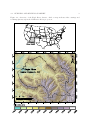
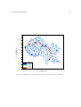
The demo dataset used in the following examples is a small tributary of the Colorado River in
the Southern Rocky Mountains, the Eagle River below Gypsum, CO, closed at USGS stream
gage 09070000 (see Figure 2.1):
Geographic coordinates:
Latitude +39◦ 38’58”
Longitude −106◦ 57’11”
NAD 1983 Albers projected coordinates:
X = −929387 m
Y = 1901293 m
Catchment area: 2445 km2
Elevation data comes from the hydro-conditioned Digital Elevation Model (DEM) provided in
the National Hydrography Dataset (NHD Plus, McKay et al., 2012 [2]), derived from the 30meter National Elevation Dataset (NED, USGS, 2009 [3]). Data files are located in the demo
directory of the toolbox.
2.1. BUILDING AND RUNNING CLARINET
9
Figure 2.1: Overview of the Eagle River dataset. Grid on map indicates false eastings and
northings (in meters) in the NAD 1983 Albers projection.
10
2.2
2.2.1
CHAPTER 2. GETTING STARTED
CLaRiNet data structures
Handling structures
The basic purpose of the CLaRiNet main library is to handle large raster datasets which would
otherwise not fit in the Scilab stack; an important part of the code is dedicated to memory
allocation and management. In order to access data from Scilab, CLaRiNet uses a system of
handles: a handle can be seen as an abstract reference to a data structure stored outside the
Scilab stack. In CLaRiNet, every handle is simply an integer identifier which is used to ’grab’
an existing data structure.
2.2.2
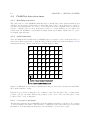
Grid indexation
Since the main library is written in C, CLaRiNet uses a row-major order for internal storage of
raster data. Indices start at 0, so that the raster cells are numbered as shown in Figure 2.2. In
many functions grid cells are referenced to by their memory offset.
Figure 2.2: Illustration of row-major cell indexation and georeferencing convention used in CLaRiNet, with a small 8 × 8 grid.
Rasters are georeferenced using the x-y coordinates of the lower-left pixel. Two conventions are
possible: (xll , yll ) can either indicate the position of the center of the lower-left pixel, or the
position of the corner of this pixel.
2.2.3
FloatRaster structure
The first data structure used in CLaRiNet is the FloatRaster structure; it is used to store arrays
of 32-bit floating-point values. The structure contains the raster data and its georeferencing
information. New FloatRaster structures can essentially be created in two ways:
11
2.2. CLARINET DATA STRUCTURES
• the function CreateFloatRaster will create a new structure with specified dimensions and
georeference information:
ras = CreateFloatRaster ( ncols, nrows, cellsize, xll, yll, NODATA_value, LL )
where LL must be either "center" (if xll and yll refer to the center of the lower-left
pixel) or "corner" (if these coordinates refer to the corner of the lower-left pixel).
• the function CreateRasterFromBinary will load a raster dataset stored in a binary file on
the disk:
ras = CreateRasterFromBinary ( binfile , datatype )
where binfile is the path (relative or absolute) to the binary file on the disk. An ascii
header file having the same and the extension .hdr must be located in the same directory
in order to provide the referencing information. The possible values for the datatype
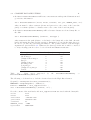
argument are given in Table 2.1. Whatever the data type in the file, it will be converted
to 4-byte floating-point in order to be stored in the FloatRaster structure.
Data type
Unsigned char
Short integer
Unsigned short integer
Integer
Unsigned integer
Floating-point
Long integer
Unsigned long integer
Double
Record size (byte)
1
2
2
4
4
4
8
8
8
Table
2.1:
Data
types
supported
CreateFlowDirFromBinary functions.
by
the
datatype argument
"uc"
"s"
"s"
"i"
"ui"
"f"
"l"
"ul"
"d"
CreateRasterFromBinary
or
The following code shows how to load the elevation data for the Eagle River dataset:
[m,path] = libraryinfo("toolbox_clarinetlib") ;
DEMOPATH = fullpath(path+"/../demos/") ;
binfile = DEMOPATH + "elev_eagleriver.flt" ;
elev = CreateRasterFromBinary ( binfile, "f" ) ;
Note the content of the ascii header file elev_eagleriver.hdr associated with the binary file:
ncols
nrows
xllcorner
yllcorner
cellsize
NODATA_value
byteorder
2772
2132
-941985.888
1856628.955
30
-9999
LSBFIRST
12
CHAPTER 2. GETTING STARTED
2.2.4
FlowDirGrid structure
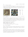
In order to perform geomorphological analyses in river networks, it is necessary to provide
information about local flow directions. CLaRiNet uses a classical D8 approach (Jenson and
Domingue, 1988 [1]) in which each pixel can flow into one of its eight neighors. You may
read/write flow direction grids from/to binary rasters using any coding convention (see Figure 2.3
for the ESRI/ArcGis convention).
23
32
61
72
59
83
65
42
32
16
16
1
64
16
1
128
26
47
65
86
90
101
71
50
64
16
32
4
4
8
1
64
31
50
70
54
53
74
107
68
4
8
2
4
4
4
8
4
17
45
64
29
36
46
79
49
16
16
1
4
16
16
16
1
35
56
63
28
34
65
111
70
64
32
4
8
8
16
16
64
45
60
22
25
37
78
83
61
4
4
8
16
16
16
2
4
26
19
55
31
76
55
67
48
4
8
16
32
16
2
4
4
18
30
51
28
56
40
31
25
8
16
1
4
16
1
1
2
Direction
→ E
ց SE
↓
S
ւ SW
← W
տ NW
↑
N
ր NE
Code
1
2
4
8
16
32
64
128
Figure 2.3: ESRI flow direction coding: elevation values (left map) and corresponding flow
directions (right map).
Because flow directions can only take 8 different values a 1-byte type is sufficient to store this
information. For this reason CLaRiNet uses a distinct data structure for storing flow direction
grids instead of the 4-byte FloatRaster structure. The following code shows how to load the
flow direction grid for the Eagle River dataset (which uses the ESRI convention) by invoking
the CreateFlowDirFromBinary function. This function creates a FlowDirGrid data structure
in memory and returns a handle on this structure in Scilab.
[m,path]=libraryinfo("toolbox_clarinetlib") ;
DEMOPATH = fullpath(path+"/../demos/") ;
fdrfile = DEMOPATH + "fdr_eagleriver.flt" ;
fdrcoding = [ 32,64,128 ; 16,255,1 ; 8,4,2 ] ;
fdr = CreateFlowDirFromBinary ( fdrfile, "f", fdrcoding ) ;
2.2.5
CellTree structure
We have seen that the flow direction grid contains the exhaustive pixel topology and that it is
sufficient to perform any search upstream or downsteam a given pixel. However, for some problems it can be usefull to translate this topological information into a different representation,
namely a binary tree.
The CellTree structure is designed for this purpose. A cell tree is always rooted at some outlet
pixel, and spans upstream from this outlet. It is a linked list in which each link contains the pixel
ID and two pointers: a pointer to its first child (i.e., the outlet of largest catchment draining into
the pixel) and a second pointer to its next sibling (i.e., the second smallest catchment draining
into the same downstream pixel). Figure 2.4 illustrates how the pixels of the catchment closed
at pixel 49 can be transformed into a binary tree.
13
2.2. CLARINET DATA STRUCTURES
0
1
2
3
4
5
6
7
8
9
10
11
12
13
14
15
16
17
18
19
20
21
22
23
24
25
26
27
28
29
30
31
32
33
34
35
36
37
38
39
40
41
42
43
44
45
46
47
48
49
50
51
52
53
54
55
56
57
58
59
60
61
62
63
Figure 2.4: Transformation of the pixel topology into a binary tree in a catchment.
14
CHAPTER 2. GETTING STARTED
This structure stores the topology in a way which avoids redundancy. Consider the tree rooted
at pixel 43:
• Pixel 43 has two children trees: the one rooted at pixel 36, and the one rooted at pixel
44 (both pixels 36 and 44 drain into pixel 43). The largest of these two trees is the one
rooted at pixel 36 (it has a total weight of 3): hence we only store the information “The
first (larger) child of pixel 43 is pixel 36”.
• Pixel 43 (which has a total weight of 6) drains into pixel 42 (its ancestor pixel); so do pixels
34 (size 1), 35 (size 14) and 51 (size 2). Hence these 4 pixels are siblings which can be
sorted by decreasing size: 35, 43, 51 and 34. Pixel 43 is second, and the only information
we need to store is: “The next sibling of pixel 43 is pixel 51”.
The most convenient aspect of this approach is that each link in the tree is a fixed-size structure
containing only static elements: an integer ID, a first pointer to the first child structure and a
second pointer to the next sibling structure. If a link has no child, then the first pointer is set
to NULL. If it has no subsequent sibling, then the second pointer is set to NULL.
A CellTree structure is created by invoking the CreateCellTree function with the handle on
flow direction grid and the outlet pixel as arguments:
[m,path]=libraryinfo("toolbox_clarinetlib") ;
DEMOPATH = fullpath(path+"/../demos/") ;
fdrfile = DEMOPATH + "fdr_eagleriver.flt" ;
fdrcoding = [ 32,64,128 ; 16,-9999,1 ; 8,4,2 ] ;
fdr = CreateFlowDirFromBinary ( fdrfile, "f", fdrcoding ) ;
header = GetFlowDirGridHeader ( fdr ) ;
outlet = XY2rec ( header, [-929387,1901293] ) ;
t = CreateCellTree ( fdr, outlet ) ;
The function returns a handle on the newly created structure, i.e. an integer ID of the tree.
Practically, besides a pixel ID and two pointers, each link of the linked list can be associated
with a weight. In the previous example, each pixel has a unit weight, so that the total weight of
the tree rooted at a given outlet is the number of upstream sites (on Figure 2.4, the tree rooted
at pixel 35 has a total weight of 14). Instead of it, the tree can be constructed with a different
weight for each pixel: this local value of the weight can be read in a raster. For example, we can
build a topographic partition based not on equal areas but on equal inflow volumes by using a
tree with the map of mean annual rainfall as a weighting raster (see Figure XX: the procedure
will be explained in Chapter 3).
2.3
2.3.1
Getting help
Online help
You can access online help either by the toolbar (or F1 shortcut), or by the prompt by typing
help followed by the name of a function:
-->help CreateFloatRaster
CLaRiNet online help provides a quite exhaustive list of the functions in the library, and a
description of their syntax.
2.4. BASIC EXAMPLES
2.3.2
15
Error messages
Thanks to the Scilab API CLaRiNet provides minimal error management. If you encounter an
error, it is often wiser to quit and restart Scilab. In some cases CLaRiNet may crash without
warning; in particular, recursive traversing in very large networks may cause stack overflow
due to an excessive recursion depth. Some important functions have dual implementations (a
recursive one and a slower, but safer, iterative one) but not all of them. In the cases where
recursive calls fail repeatedly you may want to consider splitting the problem into smaller parts,
e.g. calling the function on several subcatchments. More iterative implementations will be added
in future.
2.4
2.4.1
Basic examples
Extracting a catchment
Demo script extract_catchment.sce :
[m,path]=libraryinfo("toolbox_clarinetlib") ;
DEMOPATH = fullpath(path+"/../demos/") ;
fdrfile = DEMOPATH + "fdr_eagleriver.flt" ;
fdrcoding = [ 32,64,128 ; 16,-9999,1 ; 8,4,2 ] ;
fdr = CreateFlowDirFromBinary ( fdrfile, "f", fdrcoding ) ;
header = GetFlowDirGridHeader ( fdr ) ;
ncols = header(1);
nrows = header(2);
cellsize = header(3);
xll = header(4);
yll = header(5);
LL = header(7);
outlet = XY2rec ( header, [-929387,1901293] ) ;
// Create a new raster
NODATA_value = -9999;
bas = CreateFloatRaster(ncols,nrows,cellsize,xll,yll,NODATA_value,LL);
SetRasterToNODATA(bas);
// Flag catchment pixels with value "1" in this new raster
FlagCatchmentCells ( fdr, outlet, bas, 1 );
// Write raster to file
WriteRasterToFile(bas,DEMOPATH+"bas_eagleriver.flt");
Of course in this example we have flagged only one catchment in the raster, so it would have
made more sense to do this operation with a GIS software... However it is possible to flag as
many catchments as one wish in a single raster. We will see that this functionality will be very
usefull for generating topographic partitions (e.g. for running a spatially distributed hydrological
model).
2.4.2
Computing a hypsometric curve
Demo script hypsometric_curve.sce :
16
CHAPTER 2. GETTING STARTED
[m,path]=libraryinfo("toolbox_clarinetlib") ;
DEMOPATH = fullpath(path+"/../demos/") ;
// Run the catchment flagging script
exec(DEMOPATH+"extract_catchment.sce",-1);
// Define the empirical frequencies of the desired quantiles
P = [0:1000]/1000 ;
elev = CreateRasterFromBinary(DEMOPATH+"elev_eagleriver.flt","f");
// Compute elevation quantiles using catchment as a mask
msk = bas ;
Qz = RasterCDF(elev,msk,P);
// Plot the curve (elevations are in cm in the raster)
plot(1-P,Qz/100);
xtitle("","Exceedance probability","Elevation (m)")
The RasterCDF function can be used to compute any zonal CDF (e.g. rainfall, topographic
index, . . . ).
2.4.3
Strahler ordering
Strahler stream ordering in a catchment is a good example of a problem which is better addressed
with the use of a tree structure. The following code (demo script strahler.sce) illustrates how
to extract and order streams with a support area (threshold for channelization) of 1 km2 . The
resulting plot is shown in Figure 2.5.
[m,path]=libraryinfo("toolbox_clarinetlib") ;
DEMOPATH = fullpath(path+"/../demos/") ;
fdrfile = DEMOPATH + "fdr_eagleriver.flt" ;
fdrcoding = [ 32,64,128 ; 16,255,1 ; 8,4,2 ] ;
fdr = CreateFlowDirFromBinary ( fdrfile, "f", fdrcoding ) ;
header = GetFlowDirGridHeader ( fdr ) ;
outlet = XY2rec ( header, [-929387,1901293] ) ;
t = CreateCellTree ( fdr, outlet ) ;
cellsize = header(3) ;
pixelarea = cellsize^2 ;
supportarea = 1e6 ; // in square meters
supportweight = supportarea / pixelarea ;
[ STREAMS, StreamOrder ] = MakeStrahlerStreams ( t, supportweight ) ;
// Plot streams
COLOR = jetcolormap(max(StreamOrder));
for i=1:length(STREAMS)
XY = rec2XY(header,STREAMS(i));
order = StreamOrder(i);
plot(XY(:,1),XY(:,2),"Color",COLOR(order,:),"LineWidth",order)
end
a = gca();
a.isoview = "on";
17
2.4. BASIC EXAMPLES
1.92e+06
1.91e+06
Y, northing (m)
1.90e+06
1.89e+06
1.88e+06
1.87e+06
1.86e+06
1.85e+06
-9.4e+05
order
order
order
order
order
-9.3e+05
1
2
3
4
5
-9.2e+05
-9.1e+05
-9.0e+05
-8.9e+05
-8.8e+05
-8.7e+05
-8.6e+05
X, easting (m)
Figure 2.5: Extraction of Strahler streams for the Eagle River catchment.
18
CHAPTER 2. GETTING STARTED
Chapter 3
Writing complex workflows
19
20
CHAPTER 3. WRITING COMPLEX WORKFLOWS
Bibliography
[1] Jenson, S. K., and J. O. Domingue (1988), Extracting topographic structure from digital
elevation data for geographic information system analysis, Photogrammetric Engineering
and Remote Sensing, 54(11), 1593–1600.
[2] McKay, L., T. Bondelid, T. Dewald, et al. (2012), NHDPlus Version 2: User Guide,
ftp://ftp.horizon-systems.com/NHDPlus/NHDPlusV21/.
[3] USGS (2009), National Elevation Dataset, edition 2, U.S. Geological Survey, Sioux Fall, SD.
21