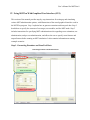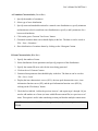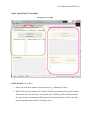
1
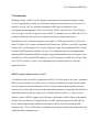
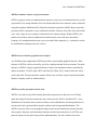
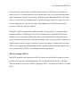
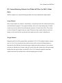
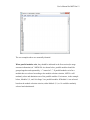
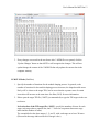
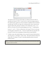
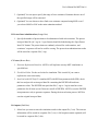
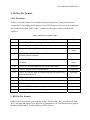
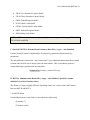
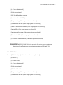
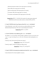
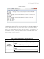
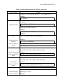
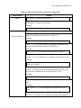
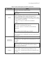
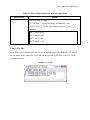
2013 User’s Manual: MSTGen Kyung (Chris) T. Han User’s Manual for MSTGen 1 Header: User’s Manual: MSTGen User’s Manual for MSTGen: Simulated Data Generator for Multistage Testing Kyung T. Han Graduate Management Admission Council ® The views and opinions expressed in this article are those of the author and do not necessarily reflect those of the Graduate Management Admission Council®. User’s Manual for MSTGen 2 I. Introduction Multistage testing, or MST, was developed as an alternative to computerized adaptive testing (CAT) for applications in which it is preferable to administer a test at the level of item sets (i.e., modules). As with CAT, the simulation technique in MST plays a critical role in the development and maintainance of tests. Theoretically, MST is a special case of CAT (likewise, CAT also can be viewed as a special version of MST). Technically, however, MST and CAT, are completely different relative to how test systems work; thus existing commercial or noncommercial CAT simulation programs, for example, CATSim (Weiss & Guyer, 2012) and SimulCAT (Han, 2012), cannot accommodate MST-based tests. MSTGen, a new MST simulation software tool, was developed to serve various purposes ranging from fundamental MST research to technical MST program evaluations. The new CAT simulation software tool supports both traditional MST functioning (MST by routing to preassembled modules after each stage; Luecht & Nungester, 1998) and new MST methods (e.g., MST by shaping a module for each stage; Han & Guo, 2012). It offers a variety of test administration environments and a user-friendly graphical interface. MSTGen supports different modes of MST Two different modes for MST are supported in MSTGen. The first mode is the typical, traditional MST in which examinees are routed to one of several preassembled test modules based on their previous responses (Luecht & Nungester, 1998). Users have three different module selection criteria to choose from (the maximum Fisher information, minimum average difficulty difference, and random selection) and can employ sets of multiple parallel modules (i.e., panels) for test exposure control. MSTGen supports up to 990 stages and modules with few limits in the number of items. The second mode is designed for the new MST approach, proposed by Han and Guo (2013), which shapes an item module for each stage on the fly, based on test information function targets. The new MST mode accomplishes item exposure control and content balancing within the module shaping process. User’s Manual for MSTGen 3 MSTGen simulates various testing environment. MSTGen supports various test administration options to create test environments that are as close as possible to live testing situations. First, the interim and final score estimates can be calculated using the maximum likelihood (ML), Bayesian maximum a posteriori (MAP), Bayes expected a posteriori (EAP) estimations, or any combination of those. Software users also can set the initial score value, range of score estimates, and restriction in estimate change. Within MSTGen, the number of test takers who are administered simultaneously at each test time slot and the frequency of communication between a test server and client computers (i.e., terminals) can also be conditioned according to the user’s choice. MSTGen has an intuitive graphical user interface As a Windows-based application, MSTGen provides a user-friendly graphical interface. Most features of MSTGen can be accessed by just a few simple point-and-click movements. The main interface of MSTGen largely retains the theme of earlier test simulation software tools that the author developed—WinGen (Han, 2007) and SimulCAT (Han, 2012), both of which are widely used in the field. The main interface consists of three easy-to-follow steps: Examinee/Item Data, Module Assembly, and Test Administration. MSTGen provides powerful research tools. MSTGen can read user-specified existing data and can generate new data sets as well. Many input and output file formats remain the same as those used in WinGen and SimulCAT . Score distribution can be drawn from a normal, uniform, or beta distribution, and item parameters for an item pool can be generated from normal, uniform, and/or lognormal distributions. The MSTGen tool also offers several graphical analysis tools such as distribution density functions, item response functions, and information functions at both item and pool levels. MSTGen can generate reports on item pool usage and test administrations. For more advanced research, User’s Manual for MSTGen 4 MSTGen provides users with options to input differential item functioning (DIF) or item parameter drift (IPD) information as well as preexisting item exposure data. The software tool also supports the use of syntax files and a cue file for massive simulation studies. System Requirements, Availability, and Distribution MSTGen runs on a Microsoft Windows-based operating system with .NET framework 2.0 or higher. Microsoft’s Windows Vista and later editions include the .NET framework, but a machine running an older version of the Windows OS will first need to have .NET framework installed. The software package, a copy of the manual in PDF format, and sample files can be found and downloaded at the following web site: http://www.hantest.net. The software package is free of charge and may be distributed to others without the author’s permission for noncommercial uses only. MSTGen always checks for the latest version and automatically updates itself as long as it is running on a machine with an active Internet connection. User’s Manual for MSTGen 5 II. MST Modes Used Within MSTGen MSTGen supports two distinctive MST modes: MST by Routing (MST-R) MST by Shaping (MST-S) MST by Routing (MST-R) As its name implies, a multistage test (MST) is divided into multiple stages and administered adaptively for each stage with a module whose difficulty level is the closest to examinee’s Module expected proficiency. For example, the following figure shows typical MST structures. Medium Stage 1 Hard Hard Medium Medium Easy Easy Stage 2 Stage 3 Test (Stage) Progress In this example, the test was divided into three stages, with one module in the first stage and three modules in each of the second and third stages. Such a design often is referred to as the “13-3” module design (Luecht, Brumfield, & Breithaupt, 2006; Jodoin, Zenisky, & Hambleton, 2006). In this design, an examinee starts with the first stage, which usually has a medium or averagee item module difficulty level. After completing the first stage, the examinee is routed in the second stage to one of three preassembled item modules, depending on his or her performance in the first stage. After completing the second stage, the examinee is, again, routed User’s Manual for MSTGen 6 to one of the three item modules in the third stage. In this way, MST behaves essentially as a special case of CAT, which adaptively routs each test taker to one of several preassembled item groups based on the test taker’s performance on the previously administered items. In the same respect, a typical CAT also resembles MST, in which each stage consists of a single item, with no items being tied to a single specific stage. This traditional type of MST hereafter will be referred to as MST by routing, or MST-R. For MST-R, MSTGen supports three different module selection criteria: (1) maximum fisher information (MFI), (2) Matching b-value, and (3) random selection. With the MFI criterion, MSTGen looks for an eligible module that results in the maximized Fisher information at the interim θ estimate after each stage. With the “matching b-value” criterion, MSTGen looks for an eligible module with an average b-value that is closest to the interim θ estimate after each stage. MSTGen also supports test administrations that have parallel modules. If parallel modules exist for a selected module, MSTGen will randomly administer one of them. MST by Shaping (MST-S) Han (2012) proposed a new approach to MST, in which a test module that is shaped as close as possible to the target test information function (TIF) is assembled on the fly after each stage. This new method is referred to as MST by shaping or MST-S. For details of the MST-S, see Han (2012). User’s Manual for MSTGen 7 III. Content Balancing Methods Used Within MSTGen (For MST-S Mode Only) MSTGen employs two content-balancing methods: the script method and weight method. Script Method In the script method, test content is controlled by a script that specifies the content area based on test administration progress. The program randomly selects one script among many available scripts to prevent test takers from predicting the sequence of content areas (Note: The current version of SimulCAT supports only one script). When the script is shorter than the actual test length, it will restart from the top after the last content area in the script is administered. Weight Method Kingsbury and Zara (1989) proposed the constrained CAT (CCAT) method to balance content areas. In CCAT, the content area from which an item will be selected for administration is determined by the difference between the target weight and actual percentage of each content area thus far administered. In other words, the system selects the content area with a percentage farthest from the target weight. For the MST-S, the CCAT method is applied to determine eligible items based on content before each item-shaping process begins. User’s Manual for MSTGen 8 IV. Using MSTGen With Graphical User Interface (GUI) This section of the manual provides step-by-step instructions for setting up and simulating various MST administration options, with illustrations of the actual graphical interface used in the MSTGen program. Step 1 explains how to generate examinee and item pool data. Step 2 details how to specify the structure of test stages, test modules, and the MST mode. Step 3 includes instructions for specifying MST administration rules regarding score estimation, test administration, and pre-test administration, and allows the user to specify extra features and output formats before running an MST simulation. It also contains information on running example scenarios. Step 1. Generating Examinee and Item Pool Data Generating Examinee and Item Pool Data User’s Manual for MSTGen 9 A. Examinee Characteristics (Green Box) 1. Specify the number of examinees. 2. Select type of score distribution . 3. Specify mean and standard deviation for a normal score distribution or, specify minimum and maximum value for a uniform score distribution or, specify a and b parameters for a beta score distribution. 4. Click on the green ‘Generate True Scores’ button. 5. Generated examinee theta scores should display in the box. The data set can be saved at ‘File > Save > Examinee.’ 6. Show distribution of examinee thetas by clicking on the ‘Histogram’ button. B. Item Characteristics (Blue Box) 1. Specify the number of items. 2. Select distribution of item parameters and specify properties of the distributions. 3. Specify the content ID (area code) for the items being generated. 4. Click on the red ‘Generate’ button. 5. Generated item parameter data should display in the box. The data set can be saved at ‘File > Save > Item.’ 6. Display the item characteristic curves (ICCs), the item pool characteristic curve, item information function curves (IIF), and the pool information function curve (PIF) by clicking on the ‘Plot Item(s)’ button. 7. Check the box labeled, ‘Add to the previous item set’, and repeat steps 1 through 4 if you need to add another set of items (or items with different content IDs) to a previous set of items. This option is useful when simulating an item pool that has multiple content areas. Note: The current version of MSTGen only supports the three parameter logistic model (3PLM). User’s Manual for MSTGen 10 Step 2. Specifying Test Assembly Specifying Test Assembly A. MST-R Mode (Green Box) 1. Select one of the three module selection criteria (e.g., Matching b-Value) 2. Either click the ‘Open Module File’ button (*.MGM) (recommended) or type the module information in the two text boxes. In a module file (*.MGM), specify information about the stage structure and modules following the format described below. (Please note that stage and module indices must be of integer value. ) User’s Manual for MSTGen 11 In Section One of the module file (*.MGM), specify module indices for each stage (each stage takes a separate line, and “:” is used as a separator between a stage index and module indices, which are delimitated by “,”). The example below includes three stages (1, 2, and 3), and a total of seven modules (Module 1 for Stage 1, Modules 2, 3, and 4 for Stage 2, and Modules 5, 6, and 7 for Stage 3). In Section Two of the module file, you need to provide the item list for each preassembled module. MSTGen supports two input methods. The first method, as shown in the example above, is to list items for each module (each module takes a separate line, and “:” is used as a separator between a module index and items, which are delimitated by “,”). The example above has 140 items, with 20 items in each module (for instance, Items 1 to 20 belonged to Module 1). To input items this way, the keyword “MI” should be placed between the first and second section of the input file. The second input method, shown in the example below, requires you to specify the module index for each item (each item takes a separate line, and “@” is used as a separator between each item and a module index). To input information this way, the keyword “IM” should be placed between the first and second section of the input file. User’s Manual for MSTGen 12 The two examples above are essentially identical. When parallel modules exist, they should be indicated in the first section (the stage structure information) of *.MGM file. As shown below, parallel modules should be grouped together and separated by “=” instead of “,”. If parallel modules exist for a module that was selected according to the module selection criterion, MSTGen will randomly select and administer one of the parallel modules. For instance, in the example below, Modules 2, 9, and 16 in Stage 2 are parallel modules. If Module 16 was selected based on the module selection criterion, either Module 2, 9, or 16 would be randomly selected and administered. User’s Manual for MSTGen 13 3. If any changes were made in the text boxes after *.MGM file was opened, click the ‘Update Changes’ button so that MSTGen will recognize the changes. This will not update/change the content of the *.MGM file but only update the current data in the computer memory. B. MST-S Mode (Pink Box) 1. Specify the number of iterations for the module shaping process. In general, as the number of iterations for the module shaping process increases, the shaped module more likely will be closer to the target TIFs, but be aware that the exposure rates of certain items also will increase at the same time. See Han (2012) for more information. 2. Either open the target TIF file (*.MGT) (recommended) or type the TIF targets in the two text boxes. In Section One of the TIF target file (*.MGT), specify the numbers of items for each stage (each stage takes a separate line, and “:” is used as a separator between a stage index and the number of items). The example below has three stages (1, 2, and 3), with each stage set to have 20 items. (Please note that stage indices must be of integer value.) User’s Manual for MSTGen 14 After the first section, the range and the number of evaluation points for the TIFs are specified in the format of “(X,Y,Z)”, where X and Y are the lower and upper bounds of the evaluation points, respectively, and Z is the number of equidistant intervals within the specified range. In MSTGen, the range of the evaluation points is always centered at the interim θ estimate after each stage. For instance, in the example above, with “(-1,1,3)” MSTGen will evaluate TIFs for the module shaping process at the “3” evaluation points between θ - 1 and θ + 1. This line is followed by a list of target TIF values for each stage (each stage takes a separate line, and “:” is used as a separator between a stage index and the target TIF values at the corresponding evaluation points [comma delimited]). 3. To balance content when module shaping, select your preferred content balancing format, either “By Script” or “By Weight,” or select “None”. The input file formats for Script and Weight differ. See Chapter V, Section 2, for detailed information about each content balancing method. NOTE: The content area (content ID) needs to be determined before the item selection criterion and exposure control are selected. User’s Manual for MSTGen 15 Step 3. Specifying MST Administration Rules Specifying MST Administration Rules A. Score Estimation (Green Box) 1. Select MLE, MAP, or EAP for estimating interim and final scores. a. Specify posterior mean and SD values if you selected MAP or EAP. (The default values for posterior mean and SD are 0 and 1, respectively). 2. Specify the initial score value. The initial score value can be fixed, randomly drawn, or loaded with a preexisting data (*.wge file). a. The default setting randomly draws a value from a uniform distribution (-0.5, 0.5). User’s Manual for MSTGen 16 3. (Optional) You can opt to specify the range of score estimates. Estimates that are out of the specified range will be truncated. 4. (Optional) You can choose to have final score estimates computed using MLE even if you selected MAP or EAP as the main estimation method. B. Pretest Item Administration (Orange Box) 1. Specify the number of pretest items to be administered with each examinee. The pretest item pool data file (in *.wgi or *.wgix format) should be loaded using the ‘Open Pretest Item File’ button. The pretest items are randomly selected for each examinee, and examinees’ responses will not be used for scoring. The pretest item administration results will be stored in a separate file (*.scp). C. Extras (Brown Box) 1. Generate Replication Data Sets. MSTGen will replicate as many MST simulations as specified here. 2. Fixed Seed Value. Fix the seed value for simulation. This is useful if you want to replicate the exact same study. 3. Item Pool with DIF/Drift. To simulate MST with DIF/item parameter drift (IPD), check this box and provide an item pool data file containing the DIF/IPD affected item parameter values. The DIF/IPD item pool data file (*.wgi or *.wgix) must have item parameters for all items (even if items are not all of DIF/IPD). MSTGen uses the DIF/IPD item parameters only to generate responses. During the item selection process, MSTGen uses the original item pool data. D. Outputs (Pink Box) 1. Select how you want to store the simulation results in the output file (*.sca). The item use information will be stored in a separate file (*.scu). A full response matrix (optional) will be stored in a separate file (*.dat). User’s Manual for MSTGen 17 E. Simulation Run (Black Box) 1. Specify the file name of the main output file (*.MGA). 2. After reviewing all your selections in Steps 1, 2, and 3, click the ‘Run Simulation’ button to launch the MST simulation. 3. Messages from MSTGen and the progress of the MST simulation will be displayed in the ‘Log/Message’ box. F. Examples To run examples, select ‘File>Open>Syntax’and choose an example syntax file. Once a syntax file is successfully loaded, review all settings throughout Steps 1, 2 and 3. Click ‘Run Simulation’ in Step 3. For more information about file formats used in MSTGen see Chapter V. For more information about MSTGen syntax commands, see Chapter VI. Example Scenario 1 (Example syntax file: MSTR1-3-3_140_MI.MGS) 1,000 examinees from a uniform distribution N(0,1) (from a data file, “10000_U_3_3.wge”) 140 items used in item modules (from a data file, “itemPool140.wgix”) MST-R Mode Stage/Module information loaded from a file, “MSTR1-3-3_140_MI.MGM”: 1-3-3 design Maximum Fisher Information Criterion for module selection Initial theta estimate is a random value between -0.5 and 0.5 Interim theta is estimated using the EAP method. Final theta is estimated using the MLE method. User’s Manual for MSTGen 18 V. MSTGen File Formats 1. File Extensions MSTGen uses and produces several kinds of input and output files. Unique extensions are assigned to files according to their purpose. Several file formats are the same as several that are used with WinGen (Han, 2007). Table 5.1 summarizes the types of files associated with MSTGen. Table 5.1 Extensions of MSTGen Files Extension Description Type *.cue SimulCAT cue file for executing sets of syntax files *.log SimulCAT log (for each ‘Run Simulation’) *.wge WinGen/SimulCAT/MSTGen data file for examinees Input and output *.wgi WinGen/ SimulCAT /MSTGen data file for item parameters (without content variables) Input only *.wgix SimulCAT/MSTGen data file for item parameters (with content variables) Input and output Input only Output only *.dat SimulCAT/ MSTGen output for full response data matrix Output only *.mga MSTGen output for MST administration Output only *.scc SimulCAT/MSTGen input for content balancing information (two different formats exist) Input only *.mgs MSTGen syntax file Input only *.mgm MSTGen module file Input only *.mgt MSTGen target TIF file Input only *.scp SimulCAT/MSTGen output for response data for pretesting items Output only *.scu SimulCAT/WinGen output for item usage information. Output only 2. MSTGen File Formats Similar to its sister programs written by the author—WinGen (Han, 2007) and SimulCAT (Han, 2012)—all input and output files in MSTGen are formatted as ASC text files and can be opened and edited with Notepad, TextPad, MS Excel, SPSS, SAS,etc. User’s Manual for MSTGen 19 A. WinGen/MSTGen Examinee Data File (*.wge)—‘tab-delimited’ Format: [Examinee #][Theta] B. WinGen/MSTGen Item Parameter Data File (*.wgi)—‘tab-delimited’ Format: [Item#][Model][# of categories][a-parameters][b-parameters][c-parameters] Models available include: 1PLM: One Parameter Logistic Model User’s Manual for MSTGen 20 2PLM: Two Parameter Logistic Model 3PLM: Three Parameter Logistic Model GRM: Graded Response Model PCM: Partial Credit Model GPCM: General Partial Credit Model NRM: Nominal Response Model RSM: Rating Scale Model NOTE: MSTGen currently does not support any polytomous response models, e.g., GRM, PCM, GPCM, NRM, and RSM. C. SimulCAT/MSTGen Extended Item Parameter Data File (*.wgix)—‘tab-delimited’ Format: [Item#][Content Code][Model][# of categories][a-parameters][b-parameters][cparameters] The only difference between the *.wgix format and *.wgi is additional information about content (content code must always be integer) after the item number. This is a mandatory format if content balancing is performed in the simulation. Example File> Example_ItemPool500.wgix D. MSTGen Administration Result File (*.mga)—‘tab-delimited’ (partially ‘commadelimited’ for a list of interim values) The format of *.mga is slightly different, depending on the user’s choice on the MST modes between MST-R and MST-S. 1. In MST-R Mode Format:[Replication # (only if there is more than one replication)] [Examinee #] [True theta value] User’s Manual for MSTGen 21 [# of items administered] [Final theta estimate] [SEE for the final theta estimate] [Administered module IDs] [Response string (if the output option was selected)] [Administered item IDs (if the output option was selected)] [Initial & interim theta estimates (if the output option was selected)] [Interim SEEs (if the output option was selected)] [Interim test information (if the output option was selected)] [True interim SEEs (if the output option was selected)] [True interim test information (if the output option was selected)] Example File> MSTR1-3-3_MI.MGA (with an option for saving response strings and administered item IDs, interim theta estimates, and interim SEEs and TIFs) 2.In MST-S Mode Format:[Replication # (only if there is more than one replication)] [Examinee #] [True theta value] [# of items administered] [Final theta estimate] [SEE for the final theta estimate] [Response string (if the output option was selected)] [Administered item IDs (if the output option was selected)] User’s Manual for MSTGen 22 [Initial & interim theta estimates (if the output option was selected)] [Interim SEEs (if the output option was selected)] [Interim test information (if the output option was selected)] [True interim SEEs (if the output option was selected)] [True interim test information (if the output option was selected)] Example File> MSTR1-3-3_MI.MGA (with an option for saving response strings and administered item IDs, interim theta estimates, and interim SEEs and TIFs) E. SimulCAT/MSTGen Item Usage (Exposure) Data File (*.scu)—‘tab-delimited’ Format: [Replication # (only if there are more than one replication)][Item #][# of item administration] [Retirement day if the item was retired during the test window] Example File> MSTR1-3-3_MI.SCU F. SimulCAT/MSTGen Content Balancing File (*.scc)—‘tab-delimited’ The formats of *.scc for ‘By Script’ and ‘By Weight’ are different. The first line should be either ‘script’ or ‘weight’, indicating the way it will be used. The format for the remaining lines is as follows: Format (by script): [Item sequence][Content area (integer)] Example File> Example_SCC_byScript.SCC Format (by weight): [Content area (integer)][weight (percent)] Example File> Example_SCC_byWeight.SCC G. SimulCAT/MSTGen Pretesting Item Administration Data File (*.scp)—‘tab-delimited’ Format: [Examinee ID (8 characters)][blank (2 spaces)] User’s Manual for MSTGen 23 [True theta value (6 characters)][blank (2 spaces)] [Final score estimate (6 characters)][blank (2 spaces)] [Response data] H. SimulCAT/MSTGen Full Response Matrix File (*.dat)—fixed format Format: [Examinee ID(8 characters)][blank (2 spaces)][Response data] Example File> MSTS6.DAT I. MSTGen Module File (*.mgm) Format: Refer to Chapter IV, Step 2.A” on page 10. Example File> MSTR1-3-3_140_MI.MGM J. MSTGen Target TIF File (*.mgt) Format: Refer to Chapter IV.Step 2.B on page 13. Example File> MSTS_targetTIFs.MGT VI. Advanced Uses of MSTGen Using a Syntax File A syntax file can be used to run MSTGen instead of the point-and-click method of the graphical user interface. Syntax files for MSTGen can be composited using any kind of text editing software such as ‘Notepad’ or ‘TextPad.’ The structure of a syntax file is straightforward—there is one command/option per line. Each line starts with an abbreviation for the corresponding section in the interface, followed by “>” and a choice of options. If an option has multiple inputs, they should be delimited by “,” (comma). See the example below for an illustration. User’s Manual for MSTGen 24 Example of Syntax File It should be noted that when MSTGen runs with a syntax file, it can only read existing data for examinee and item characteristics. To generate random examinee and/or item data, MSTGen should be used with the graphical user interface, not with a syntax file. Text/syntax after “!” is recognized as a ‘comment’ and ignored by MSTGen. Table 6.1 displays the complete list of abbreviations and options for syntax files. Table 6.1 Abbreviations/Options for MSTGen Syntax Files Abbreviation EC Option [‘file,’ a full file name with a complete directory name] Example (Examinee characteristics) IC EC> file, c:\MSTGenStudy\examinee.wge [‘file,’ a full file name with a complete directory name] Example (Item characteristics) IC> file, c:\ MSTGenStudy\item.wgix User’s Manual for MSTGen 25 Table 6.1 Abbreviations/Options for MSTGen Syntax Files Abbreviation Option [‘normal’]—scale to normal metric (D = 1.702 instead of 1.0) Example IC> normal OM (Operation mode) [‘MSTR’]—MST by Routing Example OM> MSTR !MST-R Mode [‘MSTS’, X]—MST by Shaping with X being the number of iterations for the module shaping process Example OM> MSTS, 6 !MST-S Mode with six iterations for module shaping MSC [‘MFI’]—the maximum Fisher information. (Module selection criterion) Example (Only for ‘MST-R’ mode) [‘MAT’]—the matching b-value method. ISC> MFI !MFI method [‘RAN’]—the randomization method. MGM [a full file name with a complete directory name] (Module information) (Only for ‘MST-R’ mode) Example MGM> c:\MSTGenStudy\module.mgm MGT [a full file name with a complete directory name] (Target TIF) (Only for ‘MST-S’ mode) CB Example MGT> c:\MSTGenStudy\targetTIF.mgt [‘NON’]—no content balancing (Content balancing) [‘SCR,’ a full file name with a complete directory name]—content balancing by a script. (Only for ‘MST-S’ Example User’s Manual for MSTGen 26 Table 6.1 Abbreviations/Options for MSTGen Syntax Files Abbreviation Mode) Option CB> SCR, c:\ MSTGenStudy\script.scc [‘WGT,’ a full file name with a complete directory name]—content balancing by a weight (or percentage). Example CB> WGT, c:\ MSTGenStudy\script.scc SE (Score estimation) [‘MLE’]—the maximum likelihood Estimation [‘MAP,’ X, Y]—the Bayesian maximum a posteriori estimation with a posterior distribution with mean of X and SD of Y. Example SE> MAP, 0, 1 !MAP estimation with a posteriori of N(0,1) [‘EAP,’ X, Y]—the Bayes expected a posteriori estimation with a posterior distribution with mean of X and SD of Y. Example SE> EAP, 0, 1 !EAP estimation with a posteriori of N(0,1) [‘FIX,’ X]—the initial score is fixed to X. [‘RAN,’ X, Y]—the initial score is a random value between X and Y. Example, SE> RAN, -0.5, 0.5 !Initial theta value is a random value between -0.5 and 0.5. [‘FILE,’ X, a full file name with a complete directory name]—the initial score is loaded from an existing data file (*.wge). Example, SE> FILE, c:\ MSTGenStudy\oldScore.wge [‘TRUNC,’ X, Y]—the score estimates are truncated to be between X and Y. Example, SE> TRUNC, -3, 3 !Theta estimates are truncated to be b/w -3 and 3. [‘FINAL’]—the final score is estimated using the MLE regardless of User’s Manual for MSTGen 27 Table 6.1 Abbreviations/Options for MSTGen Syntax Files Abbreviation Option the choice of proficiency estimation method. Example, SE> FINAL EXT (Extras) [‘REP,’ X]—Replicating the simulation X times. [‘DIF,’ a full file name with a complete directory name, X]— Introducing DIF/IPD from the item parameter data (*.wgi or *.wgix) for the first X number of examinees (X can be skipped if all examinees are to be introduced with DIF/IPD). [‘SEED,’ X]—Using X as a SEED value for simulation. Example, EXT> REP, 10 !Replicates 10 times EXT> DIF, c:\simulcatStudy\DIF_Param.wgi !Examinees’ responses are simulated based on the DIF item parameters. EXT> SEED, 61346125 !SEED value is 61346125 [‘IP,’ item pocket size]—simulating the worst case scenario for item pocket option. PIA (Pretest item administration) [‘NON’]— no precalibrated item to be administered. [X, a full file name with a complete directory name] – administering X pretesting items to each examinee from a pretesting item pool (*.wgi or *.wgix). Example, PIA> 5, c:\ MSTGenStudy \preTestingItems.wgi !Each examinee takes 5 precalibrated items that are randomly selected from ‘preCalItems.wgi’. OUT [’SAVE, RES’]—Saving the response strings and item IDs in *.mga. [’SAVE, THE’]—Saving all interim theta estimates in *.mga. (Outputs) [’SAVE, SEE’]—Saving all interim SEE and test information values in *.mga. [’SAVE, TRU’]—Saving all interim SEE and test information values User’s Manual for MSTGen 28 Table 6.1 Abbreviations/Options for MSTGen Syntax Files Abbreviation Option at the true theta in *.mga. [’SAVE, USE’]—Saving item usage information in *.scu. [’SAVE, FULL’]—Saving a full response matrix in *.dat. Examples OUT> SAVE, RES OUT> SAVE, THE OUT> SAVE, SEE OUT> SAVE, USE Using a Cue File A cue file is a batch file that MSTGen uses to run multiple syntax files. Basically, it is a list of the full names of the syntax files. A cue file can be executed at ‘File>Run a Cue File’ on the program menu bar. Example of a Cue File User’s Manual for MSTGen 29 References Birnbaum, A. (1968). Some latent trait models and their use in inferring an examinee’s ability. In F. M. Lord & M. R. Novick (Eds.), Statistical theories of mental test scores (Chaps. 1720). Reading, MA: Addison-Wesley. Han, K. T. (2007). WinGen: Windows software that generates IRT parameters and item responses. Applied Psychological Measurement, 31(5), 457-459. Han, K. T. (2012). SimulCAT: Windows software for simulating computerized adaptive test administration. Applied Psychological Measurement, 36(1), 64–66. Han, K. T., & Guo, F. (2013). A new approach to assembling optimal multistage testing modules on the fly. GMAC Research Report RR-13-01, March 4, 2013. Jodoin, M. G., Zenisky, A. L., Hambleton, R. K. (2006). Comparison of the psychometric properties of several computer-based test designs for credentialing exams. Applied Measurement in Education, 19, 203-220. Kingsbury, G. G., & Zara, A. R. (1989). Procedures for selecting items for computerized adaptive tests. Applied Measurement in Education, 2(4), 359–375. Luecht, R. M., & Nungester, R. (1998). Some practical examples of computer-adaptive sequential testing. Journal of Educational Measurement, 35, 239–249. Luecht, R. M., Brunfield, T., & Breithaupt, K. (2006) A testlet assembly design for adaptive multistage tests. Applied Measurement in Education, 19, 189-202. Weiss, D. J. (1982). Improving measurement quality and efficiency with adaptive testing. Applied Psychological Measurement, 6, 473–492. Weiss, D. J. & Guyer, R. (2012). Manual for CATSim: Comprehensive simulation of computerized adaptive testing. St. Paul MN: Assessment Systems Corporation. Acknowledgements The author is very grateful to Lawrence M. Rudner, Fanmin Guo, and Paula Bruggeman of the Graduate Management Admission Council® for their valuable comments and support. Author’s Address Correspondence concerning MSTGen should be addressed to Kyung T. Han, Graduate Management Admission Council, 11921 Freedom Dr., Suite 300, Reston, VA 20190; email: [email protected].