Download User Manual for the Third-Generation, Advanced Piston Corer

User Manual for the Third-Generation, Advanced Piston Corer
Temperature tool (APCT-3)
1
1
Fisher, A. T., 2Villinger, H, 2Heesemann, M.
Earth and Planetary Sciences Department and Institute for Geophysics and Planetary
Physics, University of California, Santa Cruz, CA 95064, USA
2
Department of Geosciences, Universität Bremen, Klagenfurter Straße, 28359 Bremen,
Germany
in preparation for delivery to the US-IO for IODP: (draft) XX July 2007
Acknowledgements and Preface
This document describes tools and programs that were developed in support of
international scientific drilling. Primary funds in support of this work were provided by
German Science Foundation (DFG) grants Vi 133/9-1 and Vi 133/9-2 to H. Villinger
(University of Bremen, Bremen, Germany) and by grants JSC 2-04 from the U. S.
Science Support Program to ODP and OCE-0326699 from the U.S. National Science
Foundation to A. Fisher (University of California, Santa Cruz, CA). Many individuals
contributed to this development effort, including members of the engineering and
operations groups at the U.S. Implementing Organization to IODP (formally ODP),
particularly Kevin Grigar who designed the new APCT-3 coring components and
prepared machine drawings, the tool development group at Antares (Sturh, Germany),
staff from the Scripps Institution of Oceanography Hydraulics Lababoratory, and
scientists and technicians of IODP Expedition 311. We are grateful to these individuals
for their generous contributions of time and advice, and to the US-IO to IODP for the
loan of equipment needed to develop and test the new tools.
The last generation of tools developed for measurement of temperatures while APC
coring was introduced to the scientific drilling community in 1991. Much has changed in
the last 16 years, including increasing demand for capabilities to quantify subseafloor
thermal conditions, and remarkable improvements in computational speed and electronics
stability, accuracy, and resolution. We do not imagine that this will be the last APC tool
development, or that this document will comprise the "final word" on use of the thirdgeneration tools. We encourage users to make modifications to this User Manual as
needed. If changes are made to this document, please be sure that they are carefully
noted, that all copies of the User Manual are updated, and that electronic materials are
archived.
APCT-3 User Manual
Draft: 2 July 2007
Page i
Table of Contents
Acknowledgements and Preface
Table of Contents
List of Figures
List of Tables
I. Introduction
A. Goals and Organization
B. Brief history of APCT measurements and tools
II. APCT-3 Components and Operation
A. APCT-3 Components
1. Coring hardware
2. Electronic components
B. Collecting APCT-3 Data
1. Physically preparing the APCT-3 tool
2. Programming for data collection
3. Running the station
4. Recovering the tool and data
C. APCT-3 Operation Quickstart
III. APCT-3 Data Processing
A. Modeling and other considerations
B. TP-Fit
C. APCT-3 Processing Quickstart
IV. References
Appendices
A1. APCT-3 data sheet
A2. Tool technical information
1. Coring shoe components
2. Electronics documentation
A3. Calibration
1. Goals and procedures, limitations
2. Summer 2006 calibration
A4. TP-Fit installation and operation
APCT-3 User Manual
Draft: 2 July 2007
Page ii
I. Introduction
A. Goals and Organization
This user manual accompanies the third generation of hardware and software to be
used to determine subseafloor temperatures within sediments during piston coring
operations. This manual is intended to guide shipboard scientists and technicians in (1)
the use of the APCT-3 tools to collect subseafloor thermal data, and (2) application of
software designed to help with interpretation of these data. Although it seems like it
should be a simple matter to determine the temperature of subseafloor sediments while
coring, in practice it can be challenging to collect high-quality data and interpret this data
correctly. We have attempted to explain and summarize sufficient information so that a
novice user can collect and interpret data with the APCT-3 system, but it is important to
discuss the information and recommendations in this manual with experienced scientists,
technicians, and the drilling crew.
The rest of Section I contains background information on the history of temperature
measurement while APC coring, which may be useful to know about in order to
understand why the current system was designed and constructed the way that it is. This
section also contains a few references to previous scientific and technical studies. Section
II comprises an overview of APCT-3 system components and tool operation procedures.
These are summarized at the end of this section with two "Quickstart" documents that are
intended to remind experienced users what steps to follow and in what order during
routine operation of the tools.
Section III focuses on data processing and interpretation, with an emphasis on a
newly-developed model representing tool response during deployment. The new
processing software includes a helpful graphical user interface and provides considerably
greater control on parameter selection than did earlier software, and the ability to explore
parameter dependences of extrapolated temperatures. Inexperienced users should pay
particular attention to Section IIIA, which discusses limitations of the modeling approach
and ambiguities that are likely to remain in interpretation of formation temperatures, even
when the tool is deployed properly and works well.
Section IV comprises references cited throughout the manual. Appendix A1 is the
latest version of the tool data sheet used by the US-IO when running the APCT-3.
APCT-3 User Manual
Draft: 2 July 2007
Page 1
Appendix A2 contains technical documents, machine drawings, and other information
provided by the electronics vendor. Appendix A3 comprises a discussion of APCT-3
calibration and compilation and interpretation of calibration data collected for the first
three production tool sets in Summer 2006. This information is helpful for evaluating tool
accuracy and calibration limitationsm. Appendix A4 contains installation and other
information on TP-Fit, the new APCT-3 processing program that runs through Matlab.
B. Brief history of APCT measurements and tools
Measurements of in-situ temperature have been made in oceanic sediments during
scientific drilling since before the Deep Sea Drilling Project (DSDP) began [Von Herzen
and Maxwell, 1964]. New tools were developed and modified during DSDP [Horai,
1985; Uyeda and Horai, 1980] and during the Ocean Drilling Program (ODP) [Davis et
al., 1997; Fisher and Becker, 1993; Shipboard Scientific Party, 1992a], the successor to
DSDP. In some cases, temperature tools were run during drilling programs to resolve
specific geothermal, hydrogeologic, or paleoceanographic questions, but in other cases,
data were collected during routine operations even though they were not central to
primary expedition goals (see summaries of DSDP and ODP thermal studies: [Erikson et
al., 1975; Hyndman et al., 1987; Pribnow et al., 2000]).
Temperature measurement tools in scientific ocean drilling comprise a subset of
third-party tool developments (designed, built, and tested independent of the primary
scientific operator or its subcontractors) that have contributed to both the success and the
enduring legacies of these programs. One of the most innovative down hole tool
developments in the latest years of DSDP was a piston coring shoe with temperaturemeasurement capability [Horai, 1985; Horai and Von Herzen, 1985; Koehler and Von
Herzen, 1986]. This tool allowed DSDP (and later, ODP) personnel to determine in-situ
temperatures within the undisturbed formation, well ahead of the drilling bit, without
making a dedicated tool run. These tools have been used successfully in many geological
environments to evaluate thermal conditions within sub-seafloor sediments and in open
boreholes. Although the piston coring system in DSDP was initially referred to as the
HPC, subsequent improvements created an advanced piston coring (APC) capability. A
temperature tool run with this system is herein referred to as an “APCT tool.”
APCT-3 User Manual
Draft: 2 July 2007
Page 2
Eight APCT tools based on the design introduced during DSDP were purchased by
the ODP science operator [Texas A & M University (TAMU)] in 1984 and were used
extensively during the early years of the new program. All of these tools were eventually
lost or damaged over time, and by ODP Leg 117, it was necessary to begin building a
new set of instruments. A second-generation APCT tool development was completed in
1991. This tool system was designed and built on contract by a commercial engineering
company, under the supervision of ODP personnel. The new tools were placed on the
JOIDES Resolution for use during Leg 139 and operated for over 15 years. The secondgeneration APCT tools differed from first-generation tools in several important ways.
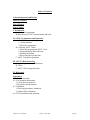
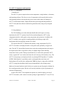
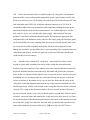
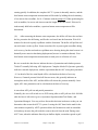
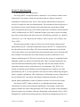
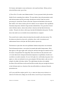
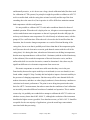
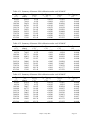
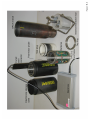
The first-generation tools were based on custom-designed and -constructed
electronics, bonded with epoxy into a form about the size of a small package of chewing
gum (Fig. I-1A). A metal probe containing a thermistor extended from the base of the
tool, and a separate battery pack was attached with a small connector. Both the tool and
battery pack fit into a slots milled into the wall of a conventional APC coring shoe. These
first-generation APCT tools were a marvel of technology, especially considering that they
were created in the early 1980's, but they were fragile instruments (particularly the
connectors) and had to be removed from the coring shoe after each deployment in order
to recover data. The second-generation tools were designed around a cylindrical tool
frame that fit into an annular cavity in the base of a redesigned APC coring shoe (Fig. I1B). Two prongs extended from the base of the tool frame, one of which contained a
platinum resistance-temperature device (RTD); the other prong helped to "register" the
tool frame as it was lowered into the annular cavity. Batteries were contained in two
separate packs that fit into the tool frame, and the tool could be programmed, deployed,
and downloaded without removing the tool from the coring shoe. As of winter 2003,
many of these second-generation tools had been lost or damaged, and the company that
had built and serviced these tools had gone out of business.
Development of a third generation of APCT tools began in 2003, with support
provided by the German Science Foundation (to H. Villinger, University of Bremen) and
the U.S. National Science Foundation (to A. Fisher, University of California, Santa
Cruz). The technical development was completed in close collaboration with Fa. Antares
(Stuhr, Germany), who had previously collaborated with H. Villinger and colleagues on
APCT-3 User Manual
Draft: 2 July 2007
Page 3
development of a Miniaturized Temperature Logger (MTL) project, for use with
collection of thermal data during conventional gravity- and piston-coring operations
(Pfender and Villinger, 2002; Jannasch et al., 2003).
Hardware designs were discussed through 2003 and into 2004, and it was decided to
retain as much as possible of the form and function of the second-generation tools, which
had proven to be robust and easy to operate. Designs for coring components were
prepared by engineers working with the U.S. Implementing Organization (US-IO) to
IODP, and new coring components were built by an established vendor. Antares
personnel created a series of prototype tool frames so that the fit into the coring
components could be confirmed, and produced a working prototype tool in advance of
IODP Expedition 311 (Cascadia Hydrates). APCT-3 project co-PIs and colleagues
worked closely with Expedition 311 researchers, who calibrated and field-tested the
prototype tool, which worked extremely well and generated useful thermal data
[Heesemann et al., 2007]. On the basis of this experience, project researchers requested
several important design and functional changes to the APCT-3 electronics, and Antares
personnel responded by producing redesigned tools in Spring 2006. These instruments
were taken to the Hydraulics Laboratory at the Scripps Institution of Oceanography in
Summer 2006 and calibrated across a working range of 0–45 °C (see Appendix A3 for a
discussion of calibration procedures and examples of results from the 2006 calibration
effort). This user manual was assembled in Spring and Summer 2007.
APCT-3 User Manual
Draft: 2 July 2007
Page 4
II. APCT-3 Components and Operation
A. APCT-3 Components
1. Introduction
The APCT-3 system comprises three main components: coring hardware, electronics,
and operating software. The first two sets of components are discussed in this section,
and operating software is discussed in the next section in the context of running an
APCT-3 measurement station. Chapter III discusses processing and interpretation of
APCT-3 data (and data collected with earlier generation tools) using newly-designed
software.
2. Coring hardware
The US-IO drilling crew and technicians handle almost all aspects of coring
operations, but APCT-3 operators benefit from understanding how APCT coring
components interface with regular coring components and operations. In addition, the
APCT-3 includes a new option for running multiple tools during a single APC
deployment; this last capability remains to be tested.
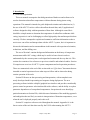
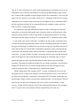
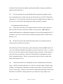
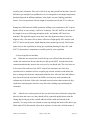
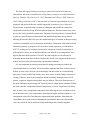
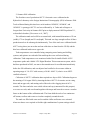
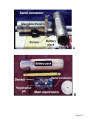
The layout of the APCT-3 illustrates the primary coring components (Fig. II-1).
APCT-3 electronics are deployed inside a coring shoe (and, optionally, an upper tool
sub). The APCT-3 shoe differs from the shoe used with second-generation tools only in
the depth extent of the o-ring surfaces (they are slightly longer) and in labeling
instructions for the vendor. During conventional use (as with earlier-generation APCT
tools) a regular APC core-catcher sub forms the seal at the top of the annular cavity. The
APCT-3 tool prototype was deployed in this way during IODP Expedition 311 and the
NGHP ("India Hydrate") expeditions, and it is anticipated that most future tool
deployments will use this same configuration. [NB: the deeper o-ring surface inside the
APCT-3 coring shoe should not lead to any incompatibilities with existing coring
hardware, but some hardware made for the new system may not fit properly with that for
the second-generation system. Be sure to fit-test any hardware as part of preparation in
advance of deployment.]
As part of the APCT-3 development, an option was created to deploy two sets of
APCT-3 electronics, with a sensor-to-sensor spacing of approximately 57.2 cm (22.5 in)
APCT-3 User Manual
Draft: 2 July 2007
Page 5
(Fig. II-1). If two electronics sets can be used simultaneously to determine correct in-situ
temperatures, this will allow determination of a thermal gradient during a single coring
run. Creation of this capability required design of three new components: cross-over sub,
upper tool sub, and a new core-catcher sub (Fig. II-1). Prototypes of the first two of these
components were created as part of the new tool development, but (as of Summer 2007)
the last component will need to be constructed before the complete system can be run
with two APCT-3 temperature loggers.
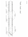
It is important to note that, although the annular cavities of the upper tool sub and
coring shoe are identical (allowing the same electronics frames to be deployed in either
location), other geometries of these components are significantly different. The coring
shoe tapers near the cutting end (Fig. II-1), placing the APCT-3 thermistor probe within
~1-2 mm of the outer surface of the shoe. In addition, the taper of the cutting shoe helps
to assure that it makes good thermal contact with the surrounding formation. In contrast,
the upper tool housing is cylindrical in cross-section (except for wrench flats that extend
across the housing 90° from the hole containing the thermistor probe), meaning that the
wall between the thermistor probe and the formation is considerably thicker than in the
coring shoe, ~8-9 mm. Perhaps of greater concern, the lack of a taper near the thermistor
probe in the upper tool sub means that the development of a damaged zone (or "skin")
outside the upper tool sub could limit the thermal contact between the tool and the
formation. The numerical models developed for use with the coring shoe, as discussed in
Chapter III, will have to be revised for interpretation of tool from the upper tool sub,
which is expected to have a somewhat slower equilibration response.
Finally, deployment of the complete APCT-3 system, including the cross-over sub
and upper tool sub, will place the butyrate core liner back about 40 cm (16 in) relative to
the front of the coring shoe, compared to conventional APC operations, making the core
pass through a longer section of metal before entering the liner. It is not known if friction
between the core and metal components will cause greater core disturbance or limit
recovery. Testing will be required to resolve this question and determine if the complete
APCT-3 system can be run routinely without compromising recovered core.
APCT-3 User Manual
Draft: 2 July 2007
Page 6
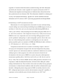
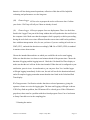
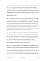
3. Electronic components
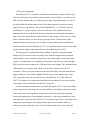
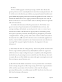
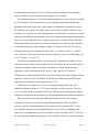
The primary APCT-3 electronics are built into an aluminum, cylindrical frame (Fig.
II-2). Four flat surfaces are machined onto the frame, two of which are currently used to
hold electronic boards, and two of which remain empty for potential future use. One of
the boards holds the measurement circuit for the thermistor probe, processor, analogdigital converter, and memory. The second board holds two 1.5-V batteries in series,
providing the 3-V power supply to the tool. On the top of the cylindrical frame are
threaded holes for use with the tool insertion-extraction tool, and female mini-banana
plug contacts for communication with the deck box and computer. There are two o-rings
on the cylindrical frame, one near the top, one near the base. On the bottom of the
cylindrical frame are two prongs, one of which is empty, and the other containing the
thermistor probe (nominal 30 kOhms at 25°C). A second thermistor or other sensor could
be placed in the empty prong as part of a later tool modification (Fig. II-2).
The electronics are programmed using a desktop or notebook computer running
Windows XP (no tests have been run using Vista; limited testing has been performed
using Windows 98, but vendor specifications do not include support for this operating
system). Communications is accomplished using serial communication, either through a
DB-9 serial port on the computer or a USB port and a serial adapter. The communications
cable attaches to a deck box, from which a second cable connects to the APCT-3
electronics. There is a special connector at the end of this cable, with male mini-banana
plugs attached to a curved form, shaped to fit into the top of the annular cavity in the
APC coring shoe when the electronics frame is installed (Fig. II-2). This allows the
APCT-3 electronics to be programmed and deployed, and data to be recovered, without
removing the electronics frame from the APC coring shoe.
A frame insertion-extraction tool is used when placing the APCT-3 electronics frame
in the coring shoe or removing it for servicing. Ideally, a tool might be placed in a coring
shoe near the start of an expedition, and not removed until the end of the expedition,
minimizing opportunities for damaging the electronics. A top ring (machined steel with
inner and outer o-rings) fits above the APCT-3 electronics frame when it is inserted in the
coring shoe, protecting the tool (and particularly the electrical contacts, which are
otherwise exposed on the top surface of the tool frame) from water, grease, and mud.
APCT-3 User Manual
Draft: 2 July 2007
Page 7
B. Collecting APCT-3 Data
1. Physically preparing the APCT-3 tool
(1a)
If you are not familiar with operation of the APCT-3 tool, take time in port or
during transit to review these instructions and run bench tests. Find an APC coring shoe
with the annular cavity and place it on the lab bench on a stand that will prevent the shoe
from falling over. The tools are kept in plastic cylinders that help to keep them clean and
prevent the electronics or prongs from being damaged. Please keep the APCT-3
electronics either inside the plastic cylinder or in an APC coring shoe; the electronics
should not be left exposed on the counter. Unscrew the top of the plastic cylinder and
remove the tool. If you just want to inspect or clean the electronics, you can extract the
frame from the plastic case by pushing your hand inside the frame, then lifting up.
However, if you are planning to insert the frame into the APC shoe, use the insertionextraction tool
(1b)
The insertion-extraction tool has two screws topped with thumb knobs that are
used to secure the tool to the electronics frame. Place the insertion-extraction tool on top
of the electronics frame and turn the thumb knobs to make up the insertion-extraction tool
tight to the frame. There are two sets of threaded holes in the top of the frame that are
compatible with the insertion tool. As of summer 2007, one set of threaded holes is
blocked (protected) with set screws, and the other set includes holes that will align the
insertion-extraction tool with the electrical contacts on the top of the tool frame. When
installed properly, a small vertical groove near the top of the insertion tool will align with
the thermistor probe, making is easier to insert the frame in the coring shoe. Before lifting
the frame using the insertion-extraction tool, back out the large wing-nut in the center of
the insertion-extraction tool so that ~3 cm of threads are exposed. This will raise a central
piston inside the insertion-extraction tool, allowing the electronics frame to be landed in
the base of the annular cavity.
(1c) Clean the o-ring grooves and clean and grease the o-rings on the electronics frame.
Use Dow 4 or similar o-ring grease.
APCT-3 User Manual
Draft: 2 July 2007
Page 8
(1d)
Before the electronics frame is installed in the APC coring shoe, the thermistor
probe should be coated with heat sink compound to assure a good contact with the shoe.
Tools were delivered to the US-IO along with a small tub of AOS non-silicone HTC heat
sink compound (part 52050-1J0), which has a thermal conductivity of 2.6 W/m-K,
considerably higher than conventional heat sink compounds. Holding the frame in one
hand with the handle on the insertion-extraction tool, use a small applicator (wooden
stick, end of a zip-tie, etc.) with the other hand to apply a thin coating of heat sink,
perhaps 1-2 mm thick, around the thermistor probe. Be sure that you apply heat sink
compound only to the thermistor probe, and not to the empty prong; the thermistor probe
can be identified by the wires extending from the main circuit board into the probe. Also
try to keep the heat sink compound on the probe. The heat sink compound will not
damage the electronics, but inevitably there is some spreading of the compound onto tool
components (and fingers), and this can make the system more difficult to handle and
could foul the electrical contacts.
(1e)
Align the probe with the APC coring shoe – there should be a short vertical
scratch or a paint mark extending from the lip of the coring shoe that indicates the
location of the hole at the base of the annular cavity into which the thermistor probe will
be placed. Hold the insertion-extraction tool by the handle and position the electronics
frame so that it is aligned with the annular cavity. It may help to have someone else hold
a flashlight or to use a camping light on your forehead during this process, so that you
can see to the base of the annular cavity. As you lower the frame into the cavity in the
coring shoe, watch the alignment mark near the top of the insertion-extraction tool. This
should align closely with the vertical mark on the coring shoe when the frame is oriented
correctly. The o-rings on the electronics frame will cause a small amount of friction as
the tool is lowered into the cavity, but you should not have to push hard. If there is much
resistance, extract the frame and examine the o-rings and cavity in the shoe to see if there
are any obstructions. If the thermistor probe lands on the bottom of the annular cavity but
misses the hole, gently raise and lower the frame until you find the hole, then lower the
frame until it lands on the bottom of the cavity. [NB: over time, the APCT shoe or
APCT-3 User Manual
Draft: 2 July 2007
Page 9
electronics frame may deform slightly, requiring that smaller o-rings (or possibly no orings) be used on the frame.]
(1f)
If you are preparing for an actual deployment (as opposed to running a bench
test), clean and dress the o-rings in the top ring. Fill out the top of an APCT Data Sheet
(Appendix A1). You will need to keep this sheet with you during the station, filling it out
as events occur, to help with data interpretation after the station is complete.
2. Programming for data collection
(2a)
Connect the serial cable to the computer and to the deck box, then connect the
deck box to the tool cable, which ends with the curved connector. [NB: Shipboard
technical staff should have configured the computer to be used for operating the APCT-3
electronics. Ask if you are not sure where to find the operating software, where to store
data files, etc.]
(2b)
Run WinTemp. Insert the mini-banana plugs on the curved connector into the
contacts on the top of the tool electronics.
In the following WinTemp instructions, typed commands are listed in bold. In almost all
cases, after entering something at the keyboard, you need to press the <enter> or <return>
key (or select the Enter button or the OK button in a pop-up window). Occasionally you
may need to press a special key or button; I’ll identify these by placing the key name
inside <triangular brackets>. Finally, you may need to select a menu or window item,
listed in this manual in italics.
(2c)
Verify that electronics are working and you have communication by choosing
Logger Online from the main menu. You will see a real-time listing of digital counts,
resistance, and temperature, updated once/second. Choose Offline to return to the main
screen. Choose Logger Battery and record the Voltage and Total Sample Count on the
Data Sheet. We don't have enough experience yet to know how long a single set of
APCT-3 User Manual
Draft: 2 July 2007
Page 10
batteries will last during normal operations; collection of this data will be helpful in
evaluating tool performance over the long term.
(2d)
Choose Logger Clear data to prepare the tool to collect new data. Confirm
your choice. WinTemp will tell you if data are already cleared.
(2e)
Choose Logger Setup to prepare for a new deployment. There is a check box
listed in the Logger Time part of the Setup window that will synchronize the tool clock to
the computer clock. Make sure that the computer clock is properly set before proceeding;
having the tool clock set at a time different from the correct time could lead to problems
later with data interpretation. Also, be sure you know if you are working in local time or
GMT (UTC), and mark the data sheet accordingly. NB: Use of GMT (UTM) is standard
in marine science observations.
Choose the intended date and time at which you would like the tool to start logging.
Make sure that this time is at least several minutes ahead of the present time. Choose the
duration of logging and the logging interval. Check the Calculated End Time display to
make sure that the tool will run for the time intended. When the tool is configured to your
satisfaction, press Activate. As an alternative, you can press Start Now! and the logger
will begin logging immediately. In this case, the tool will run for the duration indicated,
and will complete logging somewhat sooner than the time listed in the Calculated End
Time display.
WinTemp presents a Verification window that shows selected parameters, giving the
operator a chance to revise the logging plan. The time until logging will begin is shown.
If WinTemp finds no problem, the OK button will be colored green. If the OK button is
grayed out, there must be a problem with the selected program. Press Cancel and return
to Setup if needed to revise the sampling plan.
3. Running the station
APCT-3 User Manual
Draft: 2 July 2007
Page 11
(3a)
After the tool is programmed to run, remove the electrical connectors from the top
of the tool. Place the top ring (with clean, dressed o-rings) above the electronics frame.
[NB: if you insert the top ring by hand, rather than using the insertion tool, be sure that
you leave the threaded holes facing up! If you do not do this, it will be difficult to get the
top ring out later.]
(3b)
The core tech should provide a core catcher sub. Clean and dress the o-rings, then
insert the core catcher sub into the top of the coring shoe and make it up by hand so that
only a few threads remain exposed, to limit opportunities for water, dirt, or grease to foul
the electronics. Hand the untightened assembly to the core tech or another member of the
rig crew. The rig crew will tighten the core catcher prior to deployment using the special
wrench made for the APCT shoe. You will generally want to hand over the tool to the rig
crew 20–40 minutes before they send the core barrel down the pipe, and they will want to
be ready before the driller announces that the last core is on deck. The rig crew will make
up the APCT-3 coring shoe and core catcher sub to a core barrel, then will lower the
barrel into the pipe on the sand line. When the core barrel has been launched, put on your
steel-toed boots, grab a hard hat, go to the driller's shack (with the Data Sheet), and let
the driller know how you would like to run the station.
(3d)
The core barrel is usually pumped down the pipe on the sand line until the core
barrel is a few tens of meters above mudline. Let the driller know in advance if you
would like to stop at mudline to record a bottom water temperature. The APCT-3 tools
have been carefully calibrated (see Appendix A3), but it is good practice to verify bottom
water temperature at each site at least once for each electronics set used during an
expedition. More frequent bottom water measurement may be desirable, particularly
when working in shallow water or in other environments where bottom water temperature
variations are expected. The drill pipe is an efficient heat exchanger, so water in the pipe
is generally close to bottom water temperature by the time the water reaches the bottom
of the pipe, provided that the water is sufficiently deep and that the surface water is not
anomalously warm. However, depending on the pumping rate and the ambient
hydrography, water in the pipe may not equilibrate with bottom water if the pumps are
APCT-3 User Manual
Draft: 2 July 2007
Page 12
running quickly. In addition, the complete APCT-3 system is thermally massive, and the
best bottom water temperature measurement will be made by holding the tool stationary,
a few meters above mudline, for 10-15 minutes with the pumps off. When positioning the
tools at mudline, be sure to take into account the length of the core barrel. If the tool is
inadvertently held below mudline, a spurious bottom water temperature will be
determined.
(3e)
After measuring the bottom water temperature, the driller will lower the tool into
the bit, pressurize the drill string, and fire the core barrel into the formation. Wait 8-10
minutes for the tool to partly equilibrate with the formation. The driller will pull the tool
out and return it to the rig floor. Some researchers like to pause again at mudline during
tool recovery, but the tool tends to equilibrate more slowing during this time because it is
thermally more massive than during deployment (because it contains sediment). Your
best bottom water temperature measurement is made prior to collection of a core.
Be sure to mark the data sheet to indicate the time of penetration and whether pressure
"bled off" normally following APC deployment. Complete bleed off of pressure generally
indicates a normal deployment, with the expectation that the APC coring shoe penetrates
~9.5 m ahead of the bit; actual depth will be calculated on the basis of recovery.
However, if normal pressure bleed off does not occur, this generally indicates an
incomplete stroke of the APC, and the driller will release the pressure manually. Once
again, APC shoe penetration can be calculated on the basis of recovery.
A note about APC pull out and partial penetration:
Normally, the crew will switch over to XCB coring after an APC pull out of 60-100 klbs
(this decision is left to the rig crew, Operations Superintendent/Tool Pusher, and
Operations Manager). You may wish to discuss this decision in advance so that you can
determine when to run the APCT-3 system. Leaving the APC barrel in the mud for the
extra minutes required by APCT operation allows the formation to settle in around the
tool and may increase the pull needed to remove the tool from the mud. During some
APCT runs, when the sediment firmed up at shallow depths, researchers agreed to pull
APCT-3 User Manual
Draft: 2 July 2007
Page 13
out after just 6-8 minutes. If the tool is left in for any time period less than this, it may be
difficult to get enough of an equilibration curve to extrapolate a meaningful temperature,
but much depends on drilling conditions, water depth, sea state, lithology and other
factors. You can experiment with the length of measurement with the TP-Fit software.
During later ODP and early IODP operations, drilling crews continued to APC to great
depths (300 m or more) using a "drill-over" technique. The APC drill bit was advanced
the length of recovery following incomplete stroke, and another APC barrel was
launched. This approach requires more time, since the depth increment of each core
might be only a few meters, but it allows collection of high-quality APC samples, and
APCT-3 data, to much greater depths than have been attained previously. Discuss this
option early in the expedition (or during pre-expedition planning) if deep APC (and
APCT-3) penetration is important to scientific goals for your expedition.
4. Recovering the tool and data
(4a)
When the tool comes back on deck the rig crew will break the shoe and core
catcher sub connections. Be sure that they use the special APCT wrench to break the
connection and that they unscrew the cross-over by one thread only! The core techs are
well aware of the need to use the APCT wrench, but sometimes one of the lessexperienced crew members will use a regular pipe wrench, and this could deform the
shoe or damage the electronic components inside the shoe. After the shoe and sub have
been removed from the core barrel, the IODP core techs may need to hammer the
sediment out of the shoe. If the sub is loosened too much (more than one thread), they
could drive mud and grease into the cavity above the retaining ring and damage the
electronics.
(4b)
After the core catcher portion of the core has been removed from the coring shoe,
place the shoe and cross-over (they should still be connected) upside-down (with the
cutting edge facing up) on the catwalk and hose off the inside and outside of the
assembly. You may need to run a brush or some rags through the inside of the shoe to get
all the mud off. Do this outside, where there is plenty of water and it will not matter if
APCT-3 User Manual
Draft: 2 July 2007
Page 14
you make a mess. If you let the mud dry it will be tougher to clean off later. When the
shoe is clean, carry it to the lab and set it on the counter, again with the cutting edge
facing up. Wipe off the shoe and sub with a dry rag. If the sub has water on it when you
open the tool cavity, the water could drip down inside the cavity in the shoe and onto the
electronics. When the shoe and sub are clean and dry, unscrew the coring shoe. You will
need to either have someone hold the sub or put it in the vise to hold it until you get it
unscrewed past the o-rings.
(4c)
When the coring shoe is free, turn it over and place it on the stand on the counter.
If you look down inside the shoe the top ring should be visible at the top of the annular
cavity. Wipe off grease and mud from around the ring using Kimwipes, Q-tips, and rags.
Use the frame insertion-extraction tool to remove the ring, then gently wipe any water
drops off the top of the frame before attaching the electrical connector to recover the data.
NB: do not remove the APCT-3 electronics from the coring shoe unless it requires
servicing or inspection. If all goes well, you will be able to collect data from dozens of
deployments without removing the electronics from the coring shoe.
(4d)
Insert the electrical connector to allow the APCT-3 electronics to communicate
with the computer. If it is not already running, start WinTemp. Choose Logger Read
data from the main menu. If the tool is still running, you will be asked to confirm that
you would like to stop logging. You may be asked to identify a calibration file for use
with your tool. Navigate to the appropriate directory (probably C:\Program
Files\Antares)
and choose the *.wtc with the file name matching your tool number.
Data are downloaded and displayed in tabular form on the screen.
Choose File Save to save the data. The file will automatically be named with the tool
ID, followed by the date and time at which the tool started, and saved in WinTemp (.wtf)
format. It is a good idea to also save the data in text format, for use with processing
software. Choose File Export. The data will be saved to an ASCII file (.dat), using the
same naming convention. NB: WinTemp defaults to saving data to the primary Antares
directory. You can save files to a different directory, but then the program may ask you to
APCT-3 User Manual
Draft: 2 July 2007
Page 15
locate a calibration file when you next recover data. It is easier to just save to the Antares
directory, then to transfer the data to separate archive and working directories. It may be
that future releases of WinTemp provide more flexibility in file locations.
(4e)
Complete the Data Sheet, recording any anomalous events or tool behaviors. If
you plan to deploy the APCT-3 tool again soon, you can leave the APC shoe tool out on
the counter (in the stand!).
(4f)
If this is the last station for several days (or the end of the cruise), it would be a
good idea to clean up and put the tool components away for safe keeping. Use the
insertion-extraction tool to remove the electronics frame from the coring shoe. Make sure
that the central piston and shaft in the extraction tool is backed out about 3 cm by turning
the large wing-nut counter-clockwise. Lower the insertion-extraction tool onto the top of
the electronics frame and turn the thumb-knobs to engage the threaded holes in the top of
the frame. Make up the screws snug, but not too tight, so that you don't strip the threads
in the frame. If the insertion-extraction tool will not fit completely down on top of the
frame, it is likely that you need to back out the central piston and shaft by turning the
wing-nut. When the extraction tool is fully secured to the frame, turn the wing-nut
clockwise. This moves the central piston downward and pushes against the inner wall of
the coring shoe. Continuing to turn the wing-nut will "jack" the electronics frame up and
out of the cavity. Keep turning the wing-nut until the frame becomes loose, then raise the
handle on the insertion-extraction tool and gently lift the tool vertically.
(4g)
Clean the surface of the electronics gently with a dry cloth. Wipe off excess
grease or heat sink compound. Lower the clean electronics frame into the plastic
cylindrical holder and screw on the cap. Put the cylinder in a drawer or on the shelf.
Clean off the cutting shoes and sub(s). Put the interface box, cables, batteries and parts in
Ziploc bags and place these in their boxes and/or on the shelf. Tell the ET, lab tech, or
Lab Officer if supplies are needed.
APCT-3 User Manual
Draft: 2 July 2007
Page 16
C. APCT-3 Operation Quickstart
Deploy Tool (assumes electronics frame is in shoe, ready for deployment)
1. Turn on computer, launch WinTemp. Attach curved connector to top of frame.
2. Fill out top of Data Sheet.
3. Choose Logger Battery and record the Voltage and Total Sample Count on Data
Sheet.
4. Choose Logger Clear data.
5. Choose Logger Setup. Check box for Synchronize Logger from PC Time.
6. Set start time, logging duration, logging interval.
7. Press Activate and confirm plan, press OK.
8. Disconnect connector from top of frame.
9. Insert top ring. Make up core catcher sub. Hand to rig crew.
APCT-3 User Manual
Draft: 2 July 2007
Page 17
APCT-3 Operation Quickstart
Recover Tool (assumes coring shoe is clean, open, electronics frame is accessible)
1. Turn on computer, launch WinTemp. Attach curved connector to top of frame.
2. Enter time on Data Sheet.
3. Choose Logger Read Data. Confirm you wish to stop logging, if necessary.
4. Choose File Save to save the data in binary (WinTemp) format.
5. Choose File Export to save the data in ASCII format.
6. Copy and/or backup data to archive and working directories.
APCT-3 User Manual
Draft: 2 July 2007
Page 18
III. APCT-3 Data Processing
A. Modeling and other considerations
Processing APCT-3 temperature data to determine in-situ conditions cannot be done
automatically, but requires careful and somewhat subjective fitting of measured
temperatures to theoretical decay curves. Some general understanding of the physics
involved is required to make good interpretations. The description of processing steps in
the following section assumes that the reader understands the general theory behind
APCT measurement processing, as described by Horai and Von Herzen [1985] and Horai
[1985], and Heeseman et al. [2007]. Additional insight is provided by papers describing
processing of subseafloor probe data using tools with differing geometries [e.g., Bullard,
1954; Davis et al., 1997; Hartmann and Villinger, 2002; Langseth, 1965; Villinger and
Davis, 1987].
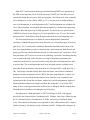
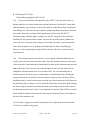
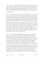
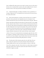
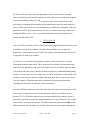
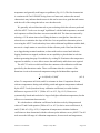
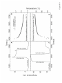
Discussing the procedure requires a brief review of tool responses during typical
deployments (Fig. III-1). Measured temperatures drop as the APCT-3 is deployed from
the ship and lowered to the seafloor. The lowest measured temperature may be found
close to the seafloor, but as described earlier, this temperature may not be consistent with
that of bottom water unless the tool is held stationary just above mud-line for 10-15
minutes with the pumps off. The tool is lowered to the bit, pressure is accumulated in the
drillstring, and the core barrel is fired into the mud. There is an abrupt temperature rise
associated with frictional heating of the coring shoe, and (for most stations) the tool
temperature begins to decay towards the true in-situ temperature (Fig. III-1A). For
stations in unusually warm sediments, the tool temperature may continue to rise after
penetration (Fig. III-1C). It is not possible to leave the tool in the seafloor long enough to
achieve complete equilibration. This would require 40-60 minutes or more, risking loss of
the tool (and the APC core barrel) with settling of sediment around the core barrel.
Instead, partial equilibration is achieved, and the core barrel is recovered by wireline.
Processing of APCT-3 data to infer the in-situ formation temperature requires
extrapolation of a short record of thermal equilibration. The programs used for this
purpose with the first- and second-generation APCT tools were based on the assumption
that tool response was consistent with a one-dimensional, radial geometry [Horai, 1985].
Fitting data to a model based on this geometry is based on the assumption (proven to be
APCT-3 User Manual
Draft: 2 July 2007
Page 19
largely appropriate) that radial heat transfer away from the tool is much more important
than vertical heat transport along the tool, and that the temperature probe is sufficiently
far from the end of the coring shoe that there is little influence associated with the
contrast in properties between the shoe and deeper sediment. As part of the development
of the APCT-3 system, new cooling curves were calculated numerically on the basis of
the geometry of the coring shoe and core barrel. In addition, earlier programs were based
on a fixed, analytical relationship between sediment thermal conductivity (k) and heat
capacity (c). New cooling curves have been calculated using a wide range of k and c
values, allowing the user to select values that seem most appropriate, and to explore the
influence of parameter selection interactively.
The general procedure is to select formation properties, select an interval of data to be
processed, and shift the tool penetration time so as to minimize the statistical misfit
between the measurements and the model. Once an appropriate fit is achieved,
temperatures are extrapolated to infinite time, using the model, to infer the in-situ
formation temperature. Users typically neglect the first 30-60 seconds of data following
penetration, as these measurements often deviate from theory for several reasons,
including the non-instantaneous and variable rate of tool penetration, and the nonuniform distribution of frictional heat. The data interval selected for processing is usually
no longer than 7-9 minutes, sometimes less, in part because of limited time with the tool
motionless in the seafloor, but also because deviations of tool cooling from the theoretical
model tend to occur at later times.
Selection of formation properties is challenging for several reasons. First, sediment
thermal conductivity is heterogeneous in many formations. Second, DSDP, ODP, and
IODP scientists typically do not determine sediment heat capacity, and there is no single
relation between thermal conductivity and heat capacity that applies for all sediments.
Third, thermal conductivity measurements are virtually never made at exactly the same
location as the temperature probe, and even if they are, recovered sediments from the
coring shoe are often highly disturbed. Thus researchers must be prepared to process data
using a variety of reasonable properties, and to list in-situ temperatures determined
through processing with uncertainties that span a range of values.
APCT-3 User Manual
Draft: 2 July 2007
Page 20
The time shift applied during processing to optimize the statistical fit between
observations and model calculations has a long history in analysis of seafloor heat flow
data [e.g., Bullard, 1954; Davis et al., 1997; Hartmann and Villinger, 2002; Langseth,
1965; Villinger and Davis, 1987]. The time shift is a heuristic representation of several
properties and processes that are virtually impossible to predict a priori: finite tool
insertion time, irregular heating, creation of a damaged zone around the coring shoe
(inside and/or outside) having different sediment properties, fluid movement away from
the tool for a brief period after penetration. Experience has shown that it is often difficult
to achieve a good fit between observations and modeled temperature decay without
allowing for the time shift. However, this additional degree of freedom in data processing
can also accommodate use of a theoretical model that is inconsistent with actual tool and
formation geometry or properties. We do not have much experience yet with the new
APCT-3 cooling curves, and there remains to be completed a detailed comparison of
older and newer decay curves and their influence on inferred in-situ temperature, but it
appears that time shifts required to "best-fit" the data using the new model may be
somewhat shorter than those needed with the older models. This suggests that the newer
models may do a better job representing experimental conditions.
It is also important in selecting a data interval during processing to examine the
experimental data very carefully, and to avoid data segments that show evidence of tool
motion. In some cases, the tool is moved abruptly and this results in a second heating
pulse that is clearly visible, but in other cases, there can be a subtle change in the rate of
cooling. If data are used in processing that include secondary heating because of tool
motion, a spurious formation temperature may be inferred. This issue illustrates one of
the great challenges in processing APCT data in general: a high-quality statistical fit does
not assure that the extrapolated formation temperature is correct. Experience has shown
that, in many cases, extrapolated temperatures from what appear to be excellent records
are inconsistent with in-situ temperatures determined at higher and lower depths (i.e., an
extrapolated value falls of an otherwise consistent thermal gradient). Sometimes the
conundrum can be resolved by reexamining the questionable data record, but in other
cases, the reason for the inconsistent extrapolated temperature remains enigmatic.
APCT-3 User Manual
Draft: 2 July 2007
Page 21
B. TP-Fit
TP-Fit is a Matlab program created for processing of APCT-3 data. Because the
geometry of the new tool is essentially identical to that of the second-generation tool, TPFit will also work with older data, provided they are properly formatted. Installation and
general Matlab and program operation are discussed in Appendix A4. In this section, it is
assumed that Matlab and TP-Fit are properly installed on the computer to be used, and
that the user has access to one or more APCT-3 data sets. Example data sets are provided
with the TP-Fit software.
As with the earlier discussion of WinTemp, instructions for TP-Fit follow some
general conventions. Typed commands are listed in bold. In almost all cases, after
entering something at the keyboard, you need to press the <enter> or <return> key (or
select the Enter button or the OK button in a pop-up window). Occasionally you may
need to press a special key or button; I’ll identify these by placing the key name inside
<triangular brackets>. Finally, you may need to select a menu or window item, listed in
this manual in italics. [NB: most TP-Fit functions can be run without the graphical user
interface, from the Matlab command line, but all instructions herein assume that the user
is running TP-Fit using the Graphical User Interface. See Appendix A4 for more
information.]
(1) Start Matlab, then cd to the working directory. This directory should contain the main
TPFit.m script and folders (subdirectories) called RefModels and TP-Fit. In general, it
will be best to have a single working directory for an expedition, and to bring data files
into this directory for processing, then move results files out of the directory when work
is complete. Be sure to follow Matlab conventions with regard to naming directories and
files (avoid spaces, unusual characters, etc.).
(2) Run TPFit from the Matlab command line. You are presented with a vertical button
window showing the typical work-flow for processing APCT-3 data. In general, buttons
will be used from top to bottom. Select Load Data to load a data file and begin
processing. When you have successfully opened an APCT data file, the Load Data and
Edit Meta-Data buttons will turn green.
APCT-3 User Manual
Draft: 2 July 2007
Page 22
(3) Choose Edit Meta-Data and enter appropriate values. Initial values are already
entered on the basis of the data file and the last values that were saved when the program
was used. In addition, values for k and c may have been set by default. Part of data
processing is evaluating the uncertainty in final temperatures caused by uncertainty in k
and c values, but it is best to enter something that you think to be reasonable. In the last
generation of APCT processing software, the user was asked to enter only a value for k,
and thermal diffusivity ( = k/c) was calculated from the empirical relation of Von
Herzen and Maxwell [1959]:
=
3.657 (k 0.70)
107
where k is in W/m-k and is in m2/s. Other studies have explored relations between k and
, and the user is advised to choose a favored relation initially, but to explore the
significance of this relation as part of APCT processing, as described below. Choose OK
to close the Edit Meta-Data window.
(4) Choose Pick to select the data segment to process, and a plot window will open
showing the complete data record. Three values must be selected: tool penetration time
(labeled t0), the initial data point to fit to the model (Data Start), and the final data point
to fit to the model (Data Stop). Because the data are shown in a standard Matlab plotting
window, you can zoom in and out, adjust axes, etc. Most of the data are colored blue, but
a subset is colored green; the latter indicates the segment of data to be processed. Zoom
in on the window of data that starts before penetration and ends after penetration,
including several minutes of data prior to tool penetration.
Press the Pick button adjacent to the t0 box, then move the cursor to the point you would
like to select to represent the time of tool penetration, and left-click with the mouse.
Because TP-Fit will shift the time between penetration and the data window as part of
processing, selection of exactly the right penetration time is not essential. TP-Fit assumes
a data window to process of 9 minutes, from 60 seconds after penetration to 600 seconds
after penetration. You can adjust one or both of these times by choosing the appropriate
APCT-3 User Manual
Draft: 2 July 2007
Page 23
Pick button, and using the cursor and mouse to select preferred times. When you have
selected all three times, press Done.
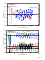
(5) Press Show Fit on the vertical button window. You are presented with a plot window
labeled Results containing four windows. The top window shows the penetration record,
with the data points used for processing colored green and red. Points not used in
processing are colored blue. Points colored red comprise the final third of the selected
data window. Also shown in the top Results window are two estimates of the equilibrium
formation temperature, labeled with green and red dashed lines. The green line is based
on the full data window, whereas the red line is based on the final third of the data
window. This plot also shows a thick gray line that falls behind the data points. This line
shows the model curve to which the observational data are compared.
The second Results window shows deviation from the model by the observations. The
deviations are plotted on a log-scale, as absolute values, with overestimates and
underestimates shown with open and filled symbols, respectively.
The bottom two plots show how the equilibrium formation temperature was estimated.
The left-bottom plot shows a cross-plot of measured and modeled temperatures. Early
data appear on the upper right corner of this plot, and later data appear towards the lower
left corner. Extrapolation of the (hopefully linear) trend shown in this plot back to the
x=0 value indicates the interpreted formation temperature at equilibrium (what the tool
would have recorded eventually, if it were left in place for a sufficiently long time). Once
again, two values are indicated, one in green using the full data window, and one in red
using the last third of the data window. The right-bottom plot shows the standard
deviation of the misfit between the model and observations (the green straight line shown
in the left-bottom plot) as a function of the time shift added to or subtracted from the
penetration time.
(6) If you would like to adjust specific k or c values, the fastest way to do this is to
return to Edit Meta-data, change one or both values, rerun Pick (you can just choose
APCT-3 User Manual
Draft: 2 July 2007
Page 24
Done immediately without changing the pick, but you must enter the Pick window), and
choose Show Fit. TP-Fit will update the results window (and plots) with your new values.
(7) If you are satisfied with the processing at this stage and would like to save your work,
use the Save Session button to put the workspace into a Matlab mat file that can be
reloaded later. You can also send results of the fit analysis to a text file for plotting with
different software by pressing Make Report.
(8) Two additional buttons are used to process APCT data using a variety of k and c
values. Press Compute Contours and the program will cycle through all available models,
using a range of k and c values, and calculate best-fitting, equilibrium temperatures for
each model. As of summer 2007, models are available for 0.5 k 2.5 W/m-k, and 2.3 x
106 c 4.3 x 106 J/m3-K, in increments of 0.1. This range of values should
accommodate the needs of most APCT-3 tool users. When the calculations are complete,
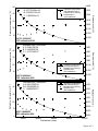
press the Explore button to see the results of the analysis. You are presented with four
contour plots in a new plot window labeled, Contours.
The top plot shows the smallest standard deviations achieved by least-squares best-fitting
of each combination of k and c values. For high-quality data (rapid tool penetration, no
motion during 8–10 minute penetration), the smallest standard deviation may be 0.01°C
or less. This is the standard deviation of a particular fit of data to a function, not an
uncertainty in the equilibrium temperature. To decide what may be an appropriate
uncertainty, look at the next plot. This one shows the equilibrium temperature as a
function of k and c. For high-quality data, there may be a range of ±0.1–0.2 °C or more
in equilibrium temperatures based on selection of reasonable values of k and c. This is a
more reasonable estimate of uncertainty in the final value (assuming high-quality data
and a good fit of observations to the model).
The third plot shows how the best-fitting time shift in penetration time varies with k and
c values, and the fourth plot shows the difference between final temperatures calculated
APCT-3 User Manual
Draft: 2 July 2007
Page 25
on the basis of the entire data window, and those based on using only the final 1/3 of the
data window.
On all contour windows, the star shows the k and c values that minimize the standard
deviation of the misfit between model and observations, and the white dot shows the
currently-selected value. If you look back at the Results window, you will see that it has
been updated to show values of k and c consistent with the position of the red star. You
can select different values of k and c by moving the cursor over the top plot on the
Contours window and left-clicking with the mouse. The white dot will move and, once
again, the Results plot is automatically updated.
(9) A few comments on selecting an equilibrium temperature. None of the information
shown on the contour plots can be used, by itself, to determine the "true" in-situ
temperature of the formation. In many cases, the properties that provide the best-fit of the
model to data may be unrealistic, for example, sometimes including very high values of k
and c. The difficulty in selecting an appropriate model (and equilibrium temperature) is
that, although the new models are better than the old models in replicating the tool
geometry, there are aspects of each deployment that remain poorly constrained,
including: the distribution of frictional heating, heterogeneities in the formation, the
quality of the thermal contact between the shoe and sensor probe, the creation of a
damaged zone around the shoe. Because these (and likely other) characteristics of each
deployment are not well characterized, available parameters (k, c, and the time shift)
may end up being "adjusted" to accommodate the data and improve the fit statistics. In
summary, a good fit of the data to the model does not demonstrate that the model (or the
equilibrium temperature) is correct. Similarly, the model that provides the statistical best
fit to the data is not necessarily most likely to be correct. Ultimately, researchers will
need to use all available data, particularly physical properties measurements from around
the APCT measurement depth, and empirical relations between k and c, and consider
whether an inferred equilibrium value makes sense on the context of other measurements.
APCT-3 User Manual
Draft: 2 July 2007
Page 26
C. APCT-3 Processing Quickstart
1. Put APCT-3 data in a working directory with the TPFit.m code (and subdirectories)
and start Matlab. Run TPFit.
2. Select Load Data to load a data file.
3. Select Edit Meta-Data and enter appropriate values. Be sure to enter values of k and c
most consistent with initial expectations.
4. Select Pick and choose the tool penetration time (t0), the initial data point to fit to the
model (Data Start), and the final data point to fit to the model (Data Stop).
5. Select Show Fit and examine the Results plot window. Return to Edit Meta-Data and
Pick as needed to examine different properties and data intervals.
6. Select Compute Contours and the program will complete the same calculations using
all available values of k and c. When this is complete, select Explore to evaluate the
influence of sediment physical properties in fit statistics, equilibrium temperatures, and
other parameters.
7. Select Save Session to create a Matlab mat file, or Make Report to generate text output
for later plotting.
APCT-3 User Manual
Draft: 2 July 2007
Page 27
IV. References
Bullard, E.C., The flow of heat through the floor of the Atlantic Ocean, Proc. Royal Soc.
Lond, Ser. A, 222, 408-429, 1954.
Davis, E.E., H. Villinger, R.D. Macdonald, R.D. Meldrum, and J. Grigel, A robust rapidresponse probe for measuring bottom-hole temperatures in deep-ocean boreholes,
Mar. Geophys. Res., 19, 267-281, 1997.
Erikson, A.J., R.P. Von Herzen, J.G. Sclater, R.W. Girdler, B.V. Marshall, and R.
Hyndman, Geothermal measurements in deep-sea drill holes, J. Geophys. Res.,
80, 2515-2528, 1975.
Fisher, A.T., and K. Becker, A guide for ODP tools for downhole measurements, pp. 148,
Ocean Drilling Program, College Station, TX, 1993.
Hartmann, A., and H. Villinger, Inversion of marine heat flow measurements by
expansion of the temperature decay function, Geophys. J. Int., 148 (3), 628-636,
2002.
Heesemann, M., H. Villinger, A.T. Fisher, A.M. Trehu, and S. Witte, Testing and
deployment of the new APC3 tool to determine insitu temperature while piston
coring, in Proc. IODP, edited by T.S. Collett, M. Riedel, and M.J. Malone, pp. in
press, Integrated Ocean Drilling Program, College Station, TX, 2007.
Horai, K., A theory of processing down-hole temperature data taken by the Hydraulic
Piston Corer (HPC) of DSDP, Lamont-Doherty Geological Observatory,
Palisades, NY, 1985.
Horai, K., and R.P. Von Herzen, Measurement of heat flow on Leg 86 of the Deep Sea
Drilling Project, in Init. Repts., DSDP, edited by G.R. Heath, and L.H. Burckle,
pp. 759-777, U. S. Govt. Printing Office, Washington, D. C., 1985.
Hyndman, R.D., M.G. Langseth, and R.P. Von Herzen, Deep Sea Drilling Project
geothermal measurements: a review, Rev. Geophys., 25, 1563-1582, 1987.
Koehler, R., and R.P. Von Herzen, A miniature deep sea temperature data recorder:
design, construction, and use, Woods Hole Oceanographic Institution, Woods
Hole, MA, 1986.
Langseth, M.G., Techniques of measuring heat flow through the ocean floor, in
Terrestrial Heat Flow, edited by W.H.K. Lee, pp. 58-77, Am. Geophys. Union,
Washington, DC, 1965.
Pribnow, D.F.C., M. Kinoshita, and C.A. Stein, Thermal data collection and heat flow
recalculations for ODP Legs 101-180., pp. <http://wwwodp.tamu.edu/publications/heatflow/>, Institute for Joint Geoscientific Research,
GGA, Hanover, Germany, 2000.
Shipboard Scientific Party, Explanatory Notes, in Proc. ODP, Init. Repts., edited by E.E.
Davis, M.J. Mottl, and A. Fisher, pp. 55-97, Ocean Drilling Program, College
Station, TX, 1992a.
Shipboard Scientific Party, Site 858, in Proc. ODP, Init. Repts.,, edited by E.E. Davis,
M.J. Mottl, and A. Fisher, pp. 431-572, Ocean Drilling Program, College Station,
TX, 1992b.
APCT-3 User Manual
Draft: 2 July 2007
Page 28
Uyeda, S., and K. Horai, Heat flow measurements on Deep Sea Drilling Project Leg 60,
in Init. Repts., DSDP, edited by D. Hussong, and S. Uyeda, pp. 789-800, U. S.
Govt. Printing Office, Washington, D. C., 1980.
Villinger, H., and E.E. Davis, A new reduction algorithm for marine heat-flow
measurements, J. Geophys. Res., 92, 12,846-12,856, 1987.
Von Herzen, R.P., and A.E. Maxwell, The measurement of thermal conductivity of deep-sea
sediments by a needle probe method, J. Geophys. Res., 64, 1557-1563, 1959.
Von Herzen, R.P., and A.E. Maxwell, Measurements of heat flow at the preliminary
Mohole site of Mexico, J. Geophys. Res., 69, 741-748, 1964.
APCT-3 User Manual
Draft: 2 July 2007
Page 29
Appendices
A1. APCT-3 data sheet
APCT-3 User Manual
Draft: 2 July 2007
Page 30
A2. Tool technical information
Documents in this section comprise an assortment of drawings, instructions, packing
slips, and other information related to APCT-3 tool components.
APCT-3 User Manual
Draft: 2 July 2007
Page 31
A3. Calibration
1. Goals and procedures, limitations
APCT-3 tool calibration is an important part of tool production and maintenance, but
there are some common misunderstandings as to the need for calibration, how it is done,
and its limitations. This section discusses these issues, and the next section reports on
results of the laboratory calibration of the first three "production" APCT-3 tools during
Summer 2006. A prototype tool was calibrated by A. Trehu and colleagues at OSU prior
to the expedition, as described in Heesemann et al. [2007].
The determination of conductive seafloor heat flow requires measurements of the
thermal gradient and thermal conductivity. What matters most from the perspective of
APCT-3 measurements used to determine the heat flux is the difference between adjacent
measurements, rather than their absolute values. However, applications involving
assessment of changes in seafloor temperature do require acquisition of absolutely
accurate data. In addition, use of multiple tools requires that data from these tools be
directly comparable; although comparison of bottom water readings provides a loose
intercalibration between tools, differences in operational procedures can make direct
comparison of apparent bottom water temperatures difficult.
As described earlier in this manual, there will always be uncertainty in estimated insitu temperatures determined with the APCT tool because many processes and properties
are not determined. Even when very high-quality data is collected, ambiguities in
processing generally result in uncertainties in equilibrium temperatures on the order of
0.1–0.2 °C. Thus the goal of calibration should be to determine the temperature recorded
with the tool at any time with an absolute accuracy at least as good as 0.01–0.02°C, and
perhaps as good as 0.002–0.004 °C. There are limited benefits to be gained from
achieving greater accuracy in calibration with this tool system.
Absoluate calibration of APCT-3 tools requires two additional instrument systems: a
stable calibration bath capable of achieving the desired temperature range, and a
precision temperature reference that has itself been calibrated to the desired accuracy
(e.g., with a NIST-traceable certificate of accuracy). Most calibration baths operate with
simultaneous water chillers and heaters that work against each other to hold the
temperature within a narrow operating range. The APCT-3 tool system is physically large
APCT-3 User Manual
Draft: 2 July 2007
Page 32
and thermally massive, so it is best to use a large, stirred calibration bath (like those used
for calibration of CTD systems). In principle it might be possible to calibrate an APCT-3
tool in a smaller bath, with the coring shoe oriented vertically and the top of the shoe
extending above the water level, but in practice it will be difficult to maintain constant
bath temperature with this configuration.
It is not possible to calibrate APCT-3 tools under conditions identical to those of
standard operation. When the tool is deployed at sea, it begins at room temperature, then
cools towards bottom water temperature as the tool is pumped down the drill pipe; the
tool may reach bottom water temperature if it is held steady at in bottom water, with the
pumps off, for a sufficient time. When the tool is lowered to the bit and fired into the
formation, the electronics changes temperature as a result of frictional heating of the
coring shoe, but at a rate that is probably much lower than that of the temperature probe
itself (because the tool electronics are not in good thermal contact with the wall of the
coring shoe). It is during this time, when the tool electronics are drifting in temperature,
that the most important data are collected for 8–10 minutes (with the tool held stationary
in the sediment). How much the temperature of the tool electronics varies, and how
uniform this drift is across the electronics, cannot be determined. Also, there may be
significant differences in electronics temperature from run to run.
Electronic components are much more stable now than they were in the past.
Functionality that used to require multi-layer circuit board (or even two boards) is now
found within a single IC chip. Certainly this has helped to improve electronic stability in
the presence of changing temperatures. But there may still be some thermal drift with
modern electronics, and there are other (largely-unknown) factors that may contribute to
variations in electronic performance. The point is not to bring into question the entire
basis for APCT-3 measurements, but rather to note that the conditions of tool calibration
are inevitably somewhat different from those of standard tool operation. This is another
reason why it is probably not worthwhile to attempt to calibrate the APCT-3 tools to an
absolute accuracy better than 0.002–0.004 °C, although the resolution of the instrument
should make higher accuracy possible. Even absolute accuracy of 0.01–0.02 °C should be
acceptable for the vast majority of applications, given the much larger uncertainties
associated with data processing.
APCT-3 User Manual
Draft: 2 July 2007
Page 33
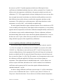
2. Summer 2006 calibration
The first three sets of production APCT-3 electronics were calibrated at the
Hydraulics Laboratory at the Scripps Institution of Oceanography (SIO) in Summer 2006.
Tools calibrated during this time have serial numbers 1858002C, 1858004C, and
1858005C. A prototype APCT-3 tool was calibrated by A. Trehu and colleagues at
Oregon State University in Summer 2005 prior to deployment on IODP Expedition 311,
as described elsewhere [Heesemann et al., 2007].
The calibration tank used at SIO was custom built, with internal dimensions of 50 cm
(width), 172 cm (length) and 36 cm (depth). This tank was large enough to allow all three
production tools to be submerged simultaneously. Two of the tools were calibrated inside
APCT coring shoes (one new shoe and one older shoe on loan from the US-IO) and the
third was calibrated inside a new upper sub.
Tank temperatures were controlled using competing water heating and chilling
systems, and spinners at each end of the tank kept the water well mixed during
calibration. Tank temperatures were monitored with a Hart Scientific Model AS125
temperature probe and a Model 1521 Digital Readout. This measurement system, which
had been purchased in 2002, was sent to the manufacturer for recalibration immediately
before the SIO calibration, and was adjusted and certified to be accurate within an
operating range of -10–50°C with accuracy of 0.001–0.002 °C (relative to an NISTcertified reference).
Collection of APCT-3 calibration data required two days at SIO. Calibration began on
the morning of 16 August 2006 by inserting the three APCT-3 electronics sets in coring
shoes and an upper sub, and starting each of the tools with a logging interval of 10
seconds. The shoes and subs were sealed with an end cap (constructed for this purpose)
or a cross-over sub, and were bound together with straps and lowered to rest on a wooden
frame on the bottom of the calibration tank. The frame held the tools a few centimeters
off bottom, to allow tank water to circulate completely around the tools.
The tank was filled with water and ice and the chiller and heater were activated.
About two hours were required to find the right combination of system settings to hold
APCT-3 User Manual
Draft: 2 July 2007
Page 34
the bath temperature constant near 0°C. Reference data were logged from the digital
probe readout by terminal emulation with a frequency of 5 seconds.
For calibration purposes, each "fixed" bath temperature was held as steady as possible
for 20–30 minutes, allowing the tools to come to thermal equilibrium with the bath.
Rheostats on the bath temperature control panel were adjusted to strengthen or weaken
the sensitivity of the heater and chiller switches in an effort to optimize stability. If the
sensitivity was set incorrectly, the bath temperature would oscillate excessively or would
drift away from the desired temperature. When we wished to change the bath temperature
(always increasing from the previous stable temperature), we turned off the chiller and
turned on the heater and watched as the bath temperature rose, then reset the controllers
to maintain temperature when a change of about 5°C had been achieved. We made no
attempt to obtain specific temperatures in the tank (e.g., exactly 15.000 °C, 20.000 °C,
etc.); instead we chose temperature increments of about 5°C across a working range of 0
to 45 °C (Tables A3-1 to A3-3).
After the first calibration point, it generally took 30–60 minutes to change to a new
temperature, and we held each temperature for 20–30 minutes. In fact, the bath could not
maintain a completely stable temperature, but tended to oscillate about the target
temperature with an amplitude of 0.005–0.010 °C and a period of 2–3 minutes.
Temperatures recorded with the ACPT-3 tools also oscillated, but with a slightly reduced
amplitude. Collection of 20–30 minutes of data for each calibration point allowed the
tank and tool oscillations to be averaged out (Fig. A3-1).
Calibration over a range of 0–30 °C was completed during the first day, and
additional calibration points at 35–45°C were completed on the second day. The tools
were recovered and data downloaded and reviewed briefly before draining the bath and
ending the calibration session, to make sure that the instrumentation worked as expected.
Data were processed to determine calibration coefficients. First, the reference
temperature records were reviewed to determine the timing of stable temperature
intervals, one for each calibration point. Next, data recovered from the APCT-3 tools
were plotted to determine tool readings during the time periods corresponding to the
times when the temperature reference was stable. Curiously, the three APCT-3 tools did
not show the same equilibration response. Tool 1858002C tended to overshoot the target
APCT-3 User Manual
Draft: 2 July 2007
Page 35
temperature and generally took longer to equilibrate (Fig. A3-1). The first characteristic
is consistent with Tool 1858002C being closer to a heater unit, whereas the second
characteristic may indicate that the sensor in this tool was not in as good thermal contact
with the wall of the coring shoe/sub as were the other tools.
We generally selected data intervals to process during which the reference probe and
all of the APCT-3 tools were in rough "equilibrium" with the bath temperature; measured
tool responses oscillated, but there was no measurable drift. The latter was assessed by
selecting a 15-20 minute interval and fitting the data to a straight line. Intervals were
selected so as to minimize the slope of this line. It is not possible to determine prior to
recovering the APCT-3 tools when they have achieved thermal equilibrium with the bath,
nor was it a simple matter to assess this with the reference probe. Data from the latter
were logged using terminal emulation, so data could not be accessed until after the
logging function was stopped, and there was no capability to plot the data in real time
without generating data gaps. Nevertheless, by waiting 20-30 minutes after temperatures
appeared to stabilize, we were able to assure that sufficiently-stable data were acquired.
The APCT-3 tools were delivered from the contractor with calibration coefficients
provided by the thermistor vendor. These coefficients relate the resistance of the
thermistor circuit to the measured temperature using the Steinhart-Hart equation:
1
= A + B(ln R) + C(ln R) 3
T
(A3-1)
where T is temperature in Kelvin, and R is resistance in ohms. Comparison of mean
reference temperatures during each stability period and apparent temperatures indicated
by the APCT-3 tools (based on factory calibration coefficients) revealed absolute
differences as great as 0.034 °C (Tables A3-1 to A3-3, Fig. A3-2). Errors were
systematically biased and tended to be largest for higher calibration temperatures, but the
offsets were inconsistent between tools.
We calculated new calibration coefficients for the three tools by fitting measured
values of T and R with equation (Tables A3-1 to A3-3) to derive new coefficients A, B,
and C (Table A3-4, Fig. A3-2). Comparison of temperatures calculated with new
coefficients to those determined with the reference probe indicates errors 0.002°C for all
tools across the full range of calibration temperatures; for most tools and temperatures,
APCT-3 User Manual
Draft: 2 July 2007
Page 36
the errors are 0.001°C. Equally important, residual errors following fit of new
coefficients are distributed randomly about zero, with no systematic bias. Curiously, for
all three tools, the temperature at which there is the greatest residual error in the new
calibration is 35°C. This suggests that the reference reading may be in error (or may have
been averaged incorrectly), but the data were checked carefully and there seems to be
little difference between the reference record for this temperature and those at other
temperatures. The residual errors at this temperature, while larger than those at other
temperatures, are still 0.002 °, well within the acceptable range.
We had originally intended to explore calibration options for use with the new ACPT3 tools, including converting directly from digital counts to temperature, or cross-plotting
apparent and true temperatures, but the basic calibration attempted initially worked out so
well, that there was no need for additional analyses. The new calibration coefficients
determined during 2006 tests have been entered into updated calibration files (*.wtc) for
the three new tools. Copies of these files are provided to the US-IO with this manual,
along with back-up copies of the original factory calibrations.
A note on updating calibration coefficients using WinTemp
WinTemp uses unique calibration coefficients associated with each tool, stored in
*.wtc files. For example, the coefficients for tool 1858002C are stored in a file called:
1858002C.wtc. When data are retrieved from an APCT-3 tool, WinTemp looks in the
current (working) directory for the appropriate file for the tool being used, and requests
that the user identify the file if it can not be found. When data are retrieved from a tool,
they are stored in a binary *.wtf file. This file contains a set of temperatures used to create
the calibration coefficients applied by WinTemp to convert from resistance to
temperature. Thus calibration data are embedded within each *.wtf file. When a user
wishes to export ASCII data, the header of the *.dat file contains a list of calibration
coefficients used to generate the file, but not the original calibration data that are
embedded within the *.wtf file.
In order to change calibration coefficients, one must open a *.wtf file, as this allows
access to a set of calibration data. Once a *.wtf file is open, choose Calibration Temperature from the main menu. You are shown a set of three resistance-temperature
APCT-3 User Manual
Draft: 2 July 2007
Page 37
(R-T) pairs, and are allowed to change these values. Apparently, WinTemp always uses
three temperatures to determine the values of the three calibration coefficients, A, B and
C. Follow these steps to get WinTemp to use coefficients determined with a greater
number of R-T pairs.
Determine coefficients based on calibration using more than three R-T pairs with a
least-squares approach (with Excel, Kaleidagraph, Matlab, or a similar program). Use a
spreadsheet to calculate three new R-T pairs using the coefficients just determined,
spanning the full range of calibration. For example, during Summer 2006 calibration, we
use a range of 0–45°C; thus we calculated three R-T pairs for T = 0, 20, 45 °C. Make sure
to cover the full calibration range, and to include values at the extreme ends and in the
middle of the range. Enter these R-T pairs in the Calibration Temperature window and
press OK. The temperature values in the open *.wtf will be updated accordingly. If you
wish to save the new calibration coefficients, choose Calibrtion Store from the main
menu, and name the *.wtc file accordingly. NB: Antares releases *.wtc files as "readonly" so you will need to change this to overwrite an existing *.wtc file. Be sure to back
up the old file first!
The method above was used for saving new coefficients based on Summer 2006
calibration of the first three APCT-3 tools. Small errors were introduced in the
specification of calibration coefficients A, B, and C (which are slightly different as stored
in the *.wtc files by WinTemp), but additional spreadsheet calculations show that these
additional errors result in calibrated temperatures that are <0.001°C different from those
determined using the full, 10-point calibration. NB: this does not mean that a 3-point
calibration is as good as a 10-point calibration! Rather, the method above "tricks"
WinTemp into using coefficients determined with a 10-point calibration, as if they were
detemined with a 3-point calibration.
APCT-3 User Manual
Draft: 2 July 2007
Page 38
Table A3-1. Summary of Summer 2006 calibration results: tool 1858002C.
Tref
(°C)
0.1992
4.9558
10.0300
14.9440
19.9130
24.9210
30.0050
35.0350
40.1180
45.1260
R002C
(ohms)
94104
74614
58654
46760
37416
30070
24232
19684
16046
13189
T002C-orig
(°C)
0.188
4.954
10.035
14.955
19.930
24.941
30.027
35.059
40.140
45.146
Tref –T002C-orig
(°C)
0.0112
0.0018
-0.0050
-0.0110
-0.0170
-0.0200
-0.0220
-0.0240
-0.0220
-0.0200
T002C-new
(°C)
0.1993
4.9561
10.0296
14.9437
19.9128
24.9209
30.0048
35.0363
40.1179
45.1255
Tref –T002C-new
(°C)
0.0001
0.0003
-0.0004
-0.0003
-0.0002
-0.0001
-0.0002
0.0013
-0.0001
-0.0005
Table A3-2. Summary of Summer 2006 calibration results: tool 1858004C.
Tref
(°C)
0.1992
4.9558
10.0300
14.9440
19.9130
24.9210
30.0050
35.0350
40.1180
45.1260
R004C
(ohms)
94211
74692
58711
46801
37445
30090
24245
19692
16050
13190
T004C-orig
(°C)
0.165
4.932
10.014
14.936
19.913
24.926
30.015
35.050
40.134
45.144
Tref –T004C-orig
(°C)
0.034
0.024
0.016
0.008
0.000
-0.005
-0.010
-0.015
-0.016
-0.018
T004C-new
(°C)
0.1990
4.9564
10.0298
14.9439
19.9130
24.9208
30.0047
35.0359
40.1177
45.1259
Tref –T004C-new
(°C)
-0.0002
0.0006
-0.0002
-0.0001
0.0000
-0.0002
-0.0003
0.0009
-0.0003
-0.0001
Table A3-3. Summary of Summer 2006 calibration results: tool 1858005C.
Tref
(°C)
0.1992
4.9558
10.0300
14.9440
19.9130
24.9210
30.0050
35.0350
40.1180
45.1260
R005C
(ohms)
93978
74535
58607
46733
37401
30063
24230
19685
16049
13193
APCT-3 User Manual
T005C-orig
(°C)
0.215
4.975
10.052
14.969
19.939
24.946
30.029
35.058
40.136
45.139
Tref –T005C-orig
(°C)
-0.0158
-0.0192
-0.0220
-0.0250
-0.0260
-0.0250
-0.0240
-0.0230
-0.0180
-0.0130
Draft: 2 July 2007
T005C-new
(°C)
0.1997
4.9561
10.0294
14.9433
19.9128
24.9210
30.0051
35.0367
40.1179
45.1252
Tref –T005C-new
(°C)
0.0005
0.0003
-0.0006
-0.0007
-0.0002
0.0000
0.0001
0.0017
-0.0001
-0.0008
Page 39
Table A3-4. Calibration coefficients for APCT-3 tools, based on fit to Steinhart-Hart
equation,
1
= A + B(ln R) + C(ln R) 3 .
T
Tool ID
A
B
-4
C
-4
1.2263852 x 10-7
1858002C
9.2779185 x 10
2.2234513 x 10
1858004C
9.3166619 x 10-4
2.2183365 x 10-4
1.2375744 x 10-7
1858005C
9.2931769 x 10-4
2.2203068 x 10-4
1.2425852 x 10-7
Notes: T is calculated in Kelvin, in ohms. Also, read section on entering coefficients
for use by WinTemp; actual coefficients used are slightly different than those listed
above, for reasons explained at the end of Appendix A3.
APCT-3 User Manual
Draft: 2 July 2007
Page 40
Figure Captions
Figure I-1. Photos of first- and second-generation APCT tools and components. A. Firstgeneration tool developed for use during DSDP (and used in the first several years of
ODP) [Horai, 1985; Horai and Von Herzen, 1985; Koehler and Von Herzen, 1986]. B.
Second-generation tool developed by Adara Systems in collaboration with ODP staff,
first deployed during ODP Leg 139 [Shipboard Scientific Party, 1992a].
Figure II-1. Machine drawing of complete APCT-3 measurement system, including
optional configuration with two electronics sets. The primary APCT-3 coring
components comprise these pieces: coring shoe with annular cavity (drawing OP4375),
cross-over sub (drawing OM0701), upper tool housing (drawing OM0702), and a corecatcher sub (drawing OM0703). Other components include o-rings and core-catcher
components, and test plugs for sealing the coring shoe and upper tool housing during lab
testing and calibration. Conventional use of the APCT-3 involves deployment of only a
single electronics set, in the coring shoe. See text for discussion of parts and deployment
options, and Appendix A2 for detailed drawings of tool components.
Figure II-2. Photo of APCT-3 electronics and related components.
Figure III-1. Examples of (second-generation) APC tool data from ODP Leg 139 in
Middle Valley [Shipboard Scientific Party, 1992b]. A. Complete deployment in relatively
cool sediments. B. Expanded view of record from in sediment, including fit of
observations to model. Every third observation is plotted for clarity. Early time data are
not used in fit because these data tend to not follow the theoretical decay curve. C.
Complete deployment in relatively warm sediments. D. Expanded view of record from in
sediment, including fit of observations to model. Every third observation is plotted for
clarity. Note how much equilibrium temperatures deviate from final in-situ temperatures,
indicating why modeling of tool response is required to estimate equilibrium tempertures.
APCT-3 User Manual
Draft: 2 July 2007
Page 41
Figure A3-1. Example calibration data from 2006 experiments with APCT-3 tools. A.
Temperatures determined with NIST-traceable reference probe. All measured values are
shown with thin line. Filled squares indicate time period during which data were
averaged to yield the mean ± standard deviation shown. The reference probe and logging
system were shut down for the night after 18:20:00, although the tank was left running to
allow work to continue the following day with minimal disruption. B. Resistances
recorded simultaneously by the three APCT-3 tools. All data recorded during the period
shown are indicated with thin lines. Symbols indicate data used to derive mean
resistances for this reference temperature, as shown. See discussion in text concerning
selection of data windows.
Figure A3-2. Calibration temperatures and residual errors plotted against tool resistance.
In all plots, the left axis shows temperature measured with the reference probe, indicated
with open squares and a thin line. The right axis shows residual errors between mean
temperatures determined with the reference probe and those determined using factory
calibrations (provided by the thermistor manufacturer, filled squares), and temperatures
determined following calculation of new Steinhart-Hart coefficients (crosses). In all
cases, the new coefficients provide residual errors 0.002 C °C. A. Tool 1858002C. B.
Tool 1858004C. C. Tool 1858005C.
APCT-3 User Manual
Draft: 2 July 2007
Page 42
30.020
Temperature (°C)
APC3 Calibration
SIO Hydraulics Lab
30.015
Point 7
T = 30.005 ± 0.004 °C
30.010
30.005
30.000
29.995
29.990
17:50:00
18:00:00
18:10:00
Time (16 August 2006)
24250
Resistance (ohms)
24245
R
APC3 Calibration
SIO Hydraulics Lab
Point 7
004C
18:20:00
18:30:00
= 94211 Ω
24240
R
24235
002C
= 94104 Ω
24230
R
24225
17:50:00
005C
= 93978 Ω
18:00:00
18:10:00
Time (16 August 2006)
18:20:00
18:30:00
Figure A3-1
40
Steinhart-Hart Coefficients:
A: 9.27791854e-04
B: 2.22345132e-04
C: 1.2263852e-07
0.040
Reference temperature
with Steinhart-Hart fit
Residual error (factory)
Residual error
(SIO calibration)
0.000
20
-0.010
-0.020
10
-0.030
40
Steinhart-Hart Coefficients:
A: 9.3166619E-04
B: 2.2183365E-04
C: 1.2375744E-07
0.030
0.020
0.010
30
0.000
Reference temperature
with Steinhart-Hart fit
Residual error (factory)
Residual error
(SIO calibration)
20
10
-0.020
-0.030
APC3 1858004C
SIO calibration 8/06
40
-0.010
Reference temperature
with Steinhart-Hart fit
Residual error (factory)
Residual error
(SIO calibration)
0.030
0.020
0.010
0.000
20
-0.010
-0.020
10
-0.030
APC3 1858005C
SIO calibration 8/06
20000
Residual misfit (°C)
Steinhart-Hart Coefficients:
A: 9.2931769E-04
B: 2.2203068E-04
C: 1.2425852E-07
30
0
Residual misfit (°C)
Reference temperature (°C)
0.020
0.010
30
APC3 1858002C
SIO calibration 8/06
Reference temperature (°C)
0.030
Residual misfit (°C)
Reference temperature (°C)
50
40000
60000
Resistance (ohms)
80000
-0.040
100000
Figure A3-2