Download ATC990/UPR900 TechNotes


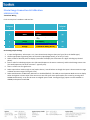
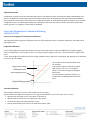
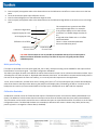
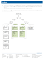
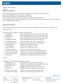
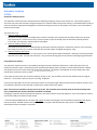
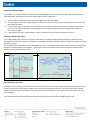
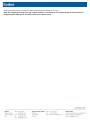
ATC
990
AND
UPR900
APPLICATIONS
AND
SETUP
Rev:
10‐22‐2013
Author:JDiOrio
ATC990
Process
Controller
and
UPR900
Process
Indicator
Technical
Notes,
Applications
and
Setup
Dynisco
UPR900
&
ATC990
Introduction
UPR900
Indicator
Is
¼
Din
(96x96mm)
size,
117mm
depth
behind
the
panel.
It
has
1
or
2
inputs
for
the
indication/display
of
pressure,
temperature
or
other
parameters.
The
graphical
display
has
80
x
160
pixels,
and
a
red/green
colour
change
backlight.
Flexible
output/option
combinations,
including
a
data
recorder
and
USB
port
Input
types
include
Strain
gauge,
linear
mA/VDC,
thermocouples
or
RTDs
ATC990
Controller
Features
and
options
are
as
on
the
UPR900,
but
with
the
addition
of
single
loop
PI/PID
control.
ATC990
has
two
very
distinct
modes
of
operation:
Pressure
or
Temperature/standard
PID.
Pressure
mode
has
options,
features,
tuning
and
calibration
tailored
to
the
specific
needs
of
the
Dynisco
core
business.
Differential
pressure
control
possible
with
the
optional
2nd
input.
The
Temperature/standard
PID
mode
offers
features
suitable
for
more
general
applications,
most
commonly
temperature:
single
PID
(heat)
or
dual
PID
(e.g.
Heat
&
Cool),
but
also
%RH,
pH
etc.
Strain
Gauge
Connection
&
Calibration
UPR900
&
ATC990
Transducer
Wiring
For
6
wire
Dynisco
Transducers
and
test
box:
Input
1
Terminal
s
Colour
2
3
4
Red
Black
White
5
6
7
Green
Blue
Orange
Function
Signal
+
Signal
‐
Excitation
+
(10VDC
+/‐
7%)
Excitation
‐
Calibration
Relay
(R‐CAL)
Calibration
Relay
(R‐CAL)
Input
2
Terminal
s
35
36
37
38
39
40
Strain
Gauge
Input
Settings
1. In
Input
Configuration,
select
Input
I
or
2,
then
choose
Strain
Gauge
as
the
Input
Type
(this
is
the
default
type).
2. Choose
appropriate
Engineering
Units
such
as
KGcm,
Mpa
(Mega
Pascal),
psi
or
bar
(or
none).
3. Select
number
of
decimal
places
to
display
(remember
the
display
has
a
maximum
of
5
digits
including
any
decimal
places).
4. Enter
a
value
for
Scale
Range
Upper
Limit
(this
would
equate
to
the
sensor
maximum),
and
the
Scale
Range
Lower
Limit
(this
would
equate
to
the
sensor
minimum
–
typically
zero).
5. There
is
a
filter
time
for
signal
noise.
6. Select
Input
Failure
mode
as
High
or
Low
(makes
alarms
/
control
behave
as
thought
the
input
is
above
maximum
range
or
below
minimum
range
if
the
signal
is
lost).
7. Select
Peak
detection
to
Maximum,
Minimum
or
Disabled
(default).
This
adds
an
extra
Operator
Mode
screen
to
display
either
the
highest
or
lowest
input
value
seen
since
it
was
last
reset.
Reset
performed
at
this
screen
by
pressing
UP
&
DOWN
simultaneously.
It
can
also
be
reset
via
a
digital
input
if
fitted.
Four
digital
(logic)
inputs
are
now
standard
on
UPR900,
and
optional
on
ATC990.
Strain
Gauge
Semi‐Automatic
Calibration
If
enabled,
the
semi‐automatic
calibration
uses
a
resistor
present
within
the
pressure
transducer,
to
calibrate
the
instrument
to
the
transducer.
The
resistor
is
used
to
force
the
mV
output
from
transducer
to
a
fixed
percentage
of
the
full
scale
value
when
the
calibration
relay
shorts
out
the
R‐CAL
connections.
Strain
Gauge
Calibration
is
a
sub‐menu
option
in
Input
Configuration,
but
can
also
be
accessed
at
any
time
by
pressing
DOWN
and
FORWARD
simultaneously.
Allow
time
for
the
instrument
and
process
to
reach
operating
temperature
before
starting.
The
first
strain
gauge
input
is
calibrated
then
the
second
if
it
is
fitted
and
configured.
1. Select
the
Shunt
Resistor
as
Enabled.
If
enabled
the
semi‐automatic
calibration
procedure
is
used.
If
it
is
disabled,
use
the
Manual
calibration
instructions
below.
2. Set
the
Calibration
Resistor
value
(default
=
80%
of
sensor
maximum).
The
instrument
must
know
what
percentage
will
be
applied
to
calibrate
correctly
–
Check
sensor
datasheet.
3. At
the
Low
Point
Calibration
screen,
ensure
the
transducer
is
at
working
temperature
with
zero
pressure
applied,
then
press
UP
and
DOWN
simultaneously.
Low
end
calibration
is
performed
and
a
completed
message
shown.
The
error
message
“Count
Failure”
is
shown
if
the
input
was
not
±10mV
of
the
nominal
0mV
expected
signal,
and
calibration
is
not
altered.
This
could
signify
a
faulty
transducer.
You
can
only
move
onto
high
end
calibration
once
the
problem
is
corrected
and
low
calibration
has
been
completed
successfully!
4. At
the
High
Point
Calibration
screen,
press
UP
and
DOWN
simultaneously.
The
calibration
relay
turns
ON
to
short
the
R‐
CAL
terminals
together
and
force
required
%mV
value
to
be
output
from
transducer
into
the
instruments
input.
High
end
calibration
is
performed
and
a
completed
message
shown.
The
error
message
“R
Cal
Failure”
is
shown
if
the
signal
was
less
than
+20mV
or
greater
than
+50mV,
and
calibration
is
not
altered.
This
could
signify
a
faulty
transducer
R‐Cal
resistor.
Repeat
the
calibration
procedure
once
the
problem
is
corrected.
5. The
procedure
from
1
to
4
is
repeated
if
a
2nd
strain
gauge
input
is
configured.
Strain
Gauge
Manual
Calibration
If
the
shunt
is
disabled,
a
Manual
Calibration
needs
to
be
performed
by
user.
Manual
Calibration
requires
the
user
to
input
known
Zero
Offset
and
Full
Scale
mV
values
into
the
input
terminals
of
the
instrument
using
an
accurate
mV
calibration
source.
The
Manual
Calibration
process
for
the
low
offset
is
as
follows:
1. Ensure
Unit
is
powered
on
and
mV
Input
from
the
calibration
signal
source
is
wired
to
the
instrument’s
strain
gauge
input
terminals.
2. Enter
the
Strain
Gauge
Calibration
mode,
(e.g.
press
DOWN
and
FORWARD
simultaneously).
3. Select
the
Shunt
Resistor
as
Disabled.
4. The
Calibration
Resistor
percentage
value
is
fixed
to
100.0%
and
cannot
be
changed
by
the
user.
5. At
the
Low
Point
Calibration
screen,
check
that
the
calibration
signal
is
set
to
exactly
the
transducer
mV
signal
at
zero
pressure,
then
press
UP
and
DOWN
simultaneously.
Low
end
calibration
is
performed
and
a
completed
message
shown.
The
error
message
“Count
Failure”
is
shown
if
the
input
was
not
±10mV
of
the
nominal
0mV
expected
signal,
and
calibration
is
not
altered.
Check
your
signal
and
repeat
the
calibration
process
from
the
start.
You
can
only
move
onto
high
end
calibration
once
low
calibration
has
been
completed
successfully!
6. At
the
High
Point
Calibration
screen,
check
that
the
calibration
signal
is
set
to
the
full
scale
mV
signal
as
per
the
transducer
datasheets
(e.g.
33.3mV),
then
press
UP
and
DOWN
simultaneously.
High
end
calibration
is
performed
and
a
completed
message
shown.
The
error
message
“R
Cal
Failure”
is
shown
and
calibration
is
not
altered
if
the
signal
was
less
than
+20mV
or
greater
than
+50mV
OR
the
High
Cal
–
Low
Cal
value
is
less
than
10mV.
Check
your
signal
and
repeat
the
calibration
process
from
the
start.
Calibration
Reminder
A
calibration
reminder
can
be
set
if
Data
Recorder
option
is
fitted
(which
means
instrument
has
battery‐backed
Real
Time
Clock).
The
addition
of
a
clock
means
that
the
instrument
can
be
aware
of
the
date
and
time
(even
when
powered
down).
This
information
can
be
used
to
remind
the
user
to
calibrate
the
inputs
at
a
specified
future
date.
The
date
is
set
in
the
Input
Configuration
menu.
If
enabled
and
the
date
set
is
exceeded,
a
calibration
due
screen
is
shown
every
24hrs
(and
at
every
power‐up)
until
it
is
changed
to
a
future
date
(or
disabled).
Linear
and
Temperature
Calibration
&
Scaling
UPR900
&
ATC990
Linear
(non‐strain
gauge)
and
Temperature
Calibration
The
instrument
offers
single
point
calibration,
with
zero
offset
adjustment
only,
or
two
point
calibration,
with
both
zero
&
span
adjustments.
Single
Point
Calibration
A
‘zero
offset’
applied
to
the
process
variable
across
the
entire
span.
Positive
values
are
added
to
the
reading,
negative
values
are
subtracted.
Can
be
used
if
the
error
is
constant
across
the
range,
or
the
user
is
only
interested
in
a
single
critical
value.
To
use,
select
Single
Point
Calibration
from
the
input
calibration
menu,
and
enter
a
value
equal,
but
opposite
to
the
observed
error
to
correct
the
reading.
This
example
shows
a
positive
offset
value.
For
example:
If
the
process
displays
27.8
when
it
should
Single
Point
‘Offset
read
30,
The
error
is
‐2.2
so
an
applied
Calibration’
value
offset
of
+2.2
would
change
the
displayed
value
to
30.
New
Displayed
Value
The
same
offset
is
applied
to
all
values,
so
at
100.0
the
new
displayed
value
would
be
102.2.
Original
Displayed
Value
Two
Point
Calibration
This
method
is
used
where
an
error
is
not
constant
across
the
range.
Separate
offsets
are
applied
at
two
points
in
the
range
to
eliminate
both
“zero”
and
“span”
errors.
To
use:
1. Measure
and
record
the
error
at
a
low
point
in
the
process.
2. Measure
and
record
the
error
at
a
high
point
in
the
process.
3. Go
to
the
first
two
point
input
calibration
screen.
a. Enter
the
desired
low
point
value
as
the
Calibration
Low
PV
value.
b. Enter
an
equal,
but
opposite
value
to
the
observed
error
as
the
Calibration
Low
Offset
to
correct
the
error
at
the
low
point.
4. Go
to
the
second
two
point
input
calibration
screen.
a. Enter
the
desired
high
point
as
the
Calibration
High
PV
value.
b. Enter
an
equal,
but
opposite
value
to
the
observed
error
as
the
Calibration
High
Offset
to
correct
the
error
at
the
high
point.
This
example
shows
a
positive
Low
Offset
and
a
negative
High
Offset.
For
example:
Calibration
High
Offset
If
the
process
displays
+0.5
at
the
low
end,
Original
Displayed
Value
an
offset
of
‐0.5
would
change
the
value
to
0.0
New
Displayed
Value
A
high
end
value
of
98.3
with
a
+1.7
offset
would
read
100.0.
Calibration
Low
Offset
There
is
a
linear
relationship
between
these
two
calibration
points.
Calibration
Low
Process
Value
Calibration
Low
Process
Value
CAUTION:
Choose
values
as
near
as
possible
to
the
bottom
and
top
of
your
usable
span
to
achieve
maximum
calibration
accuracy.
The
effect
of
any
error
can
grow
past
the
chosen
calibration
points.
Multi‐point
Scaling
If
an
input
is
connected
to
a
linear
input
signal
(mA,
mV
or
VDC),
multi‐point
scaling
can
be
enabled
for
that
input
to
allow
linearization
of
a
non‐linear
signal.
–
see
Input
Configuration
Sub‐Menu.
The
Scale
Input
Upper
&
Lower
Limits
define
the
values
shown
when
the
input
is
at
its
minimum
and
maximum
values.
Up
to
15
breakpoints
can
scale
the
input
vs.
displayed
value
between
these
limits.
It
is
advisable
to
concentrate
the
break
points
in
the
area
of
the
range
with
the
most
non‐linearity,
or
an
area
of
particular
importance
to
the
application.
To
use,
set
the
scale
limits,
and
then
enter
the
1st
scaling
point
(this
is
a
%
of
the
scaled
input
span,
and
the
desired
display
value
to
be
shown
at
that
input
value.
Next
set
the
2nd
point
and
display
value,
followed
by
the
3rd
etc.
Continue
unit
all
breakpoints
are
used
or
you
have
reached
100%
of
the
input
span.
A
breakpoint
set
at
100%
ends
the
sequence
Calibration
Reminder
A
calibration
reminder
can
be
set
if
Data
Recorder
option
is
fitted
(which
means
instrument
has
battery‐backed
Real
Time
Clock).
The
addition
of
a
clock
means
that
the
instrument
can
be
aware
of
the
date
and
time
(even
when
powered
down).
This
information
can
be
used
to
remind
the
user
to
calibrate
the
inputs
at
a
specified
future
date.
The
date
is
set
in
the
Input
Configuration
menu.
If
enabled
and
the
date
set
is
exceeded,
a
calibration
due
screen
is
shown
every
24hrs
(and
at
every
power‐up)
until
it
is
changed
to
a
future
date
(or
disabled).
Setting
Up
ATC990
for
Use
Pressure
Setup
&
Automatic
Tuning
&
Operation
1. Power
up
the
instrument
and
if
in
automatic
control
mode(1.),
change
to
manual
mode
at
0%
power/0
RPM(2)..
Set
the
alarm
types
and
values
as
required
for
your
application
(see
alarm
configuration).
2. Set
local
setpoint
1
as
the
active
setpoint,
and
its
value
to
the
required
operating
pressure(3).
3. Allow
the
process
to
reach
operating
temperature,
then
carefully
adjust
the
manual
power
level
(use
UP
&
DOWN
keys
from
the
main
screen)
to
bring
the
process
approximately
to
the
operating
pressure.
4. Select
the
automatic
tuning
menu,
and
set
“Run
Pressure
Pre‐Tune”
to
YES.
5. Press
the
RIGHT
key.
The
Pressure
Tune
Status
screen
shows
the
current
status
‐e.g.
“Running”,
and
The
TUNE
LED
is
flashes
until
the
pre‐tune
is
completed.
6. The
instrument
adds
the
defined
Pressure
Tune
Output
pulse(4.)
to
the
current
manual
power
level,
the
process
reaction
is
observed
and
the
instrument
calculates
and
stores
the
correct
PI
tuning
terms.
Pre‐tune
is
now
complete
and
exits.
7. Automatic
control
can
now
be
selected,
where
the
control
power
output
level
is
maintained
by
the
controller.
If
setpoint
mode
was
selected
as
the
auto/manual
transfer
method,
some
adjustment
of
the
setpoint
may
be
required(5.).
8. Optionally
Pressure
Self‐Tune
may
be
used
once
in
automatic
control
mode,
by
selecting
the
automatic
tuning
menu,
and
setting
“Run
Pressure
Self‐Tune”
to
YES(6.).
The
TUNE
LED
is
lit
if
Self‐tune
is
enabled.
Notes
for
Setup
&
Automatic
Tuning
&
Operation
1. The
initial
“power‐up
control
state”
can
be
set
to
manual
or
automatic
from
the
control
configuration
menu,
the
default
is
manual
mode
at
0%
power(2)..
Auto
or
manual
mode
can
be
selected
from
the
auto/manual
control
menu,
or
to
immediately
go
to
manual
mode
from
any
point,
simply
press
the
LEFT
&
RIGHT
keys
simultaneously.
The
transition
from
auto
to
manual
control
while
running
is
Bumpless.
It
takes
the
last
PI
power
level
as
the
initial
manual
control
power
level.
2. Manual
power
can
be
expressed
in
%
or
RPM.
For
RPM,
enable
“Scaled
Power”
in
the
control
configuration
menu,
then
scale
0%
and
100%
power
to
their
equivalent
RPM
values).
3. Setpoint
Select
and
the
setpoint
value
screen
is
in
operation
mode.
Setpoint
upper
and
lower
limits
can
be
set
in
the
control
configuration
menu.
4. The
Pressure
Tune
Output
pulse
value
is
set
in
the
control
configuration
menu.
The
pulse
can
be
from
‐25%
to
+25%.
Default
is
10%.
5. The
method
of
transition
from
manual
to
automatic
control
is
set
in
the
control
configuration
menu.
Two
methods
are
possible,
both
ensure
a
smooth
transition
to
automatic
mode:
a. Bumpless
Mode
sets
the
initial
PI
power
level
to
match
the
previous
manual
power
vale,
then
uses
the
integral
function
progressively
alter
the
power
to
the
correct
value.
b. Setpoint
Mode
modified
the
current
Setpoint
value
to
the
measured
input
pressure
value
at
the
time
of
switchover.
The
operator
can
change
the
setpoint
value
from
the
setpoint
value
screen
and
the
PI
control
algorithm
will
adjust
the
process
to
this
value.
6. The
self‐tune
is
a
continuous,
on
on‐line
algorithm
that
"observes"
the
measured
value
and
looks
for
oscillation
due
to
load
variations
or
set‐point
changes.
When
a
significant
pattern
is
recognized
the
tuning
parameters
are
automatically
adjusted.
When
Self‐tune
is
running
the
PI
parameters
(PB,
TI)
are
read
only
in
the
operator
menus.
The
type
of
automatic
tuning
available
depends
on
which
mode
the
controller
is
in
(Pressure
or
Non‐Pressure),
and
whether
the
control
is
manual
or
automatic.
Alarms
&
Latching
Outputs
UPR900
Alarms
In
Alarm
Configuration,
there
are
up
to
3
alarms
selectable
as
Process
High,
Process
Low,
Rate
of
Signal
Change
(per
minute),
Sensor/input
Break,
The
alarm
source
can
be
input
1
or
2
Enter
the
value
(threshold)
at
which
the
alarm
should
occur,
an
adjustable
hysteresis
value
and
an
alarm
filter
time
(this
is
the
minimum
duration
for
on
to
happen,
but
if
set
to
OFF
activation
is
immediate).
There
is
also
an
option
to
inhibit
(mask)
an
alarm
at
power‐up.
Colour
change
on
alarm
is
optional
(set
in
Display
Configuration)
Outputs
Only
relays
can
be
used
as
alarm
outputs.
In
Output
Configuration,
select
a
relay
output
to
use,
then
select
Alarm
1,
2
or
3
(direct
or
reverse
acting).
Alternatively,
select
Boolean
logical
output
of
alarms
1
OR
2,
or
alarms
1,
2
OR
3
(these
also
can
be
direct
or
reverse
acting).
Reverse
action
with
OR
would
equate
to
Boolean
NOR.
Each
output
can
be
selected
to
latch
or
not
independently.
Usage
If
the
alarm
threshold
is
exceeded
for
longer
than
the
filer
time
(assuming
no
power‐up
inhibit),
the
alarm
activates,
and
relay
changes
state.
NOTE:
from
normal
main
operator
screen,
pressing
the
BACK
key
shows
the
Alarm
Status
Screen,
and
another
press
will
show
the
Clear
Latched
Outputs
screen
(if
any
are
latched).
When
alarm
threshold
is
no‐longer
exceeded,
the
alarm
turns
off
and
a
non‐latching
relay
output
would
also
change
back.
However,
if
the
relay
output
was
set
for
latching
it
would
not
change
back.
At
the
Clear
Latched
Outputs
screen,
use
FORWARD
or
BACK
keys
to
select
the
latched
outputs,
then
press
the
UP
or
DOWN
key
to
unlatch
it.
NOTE:
The
output
can
only
be
unlatched
if
the
associated
alarm
is
no‐longer
active.
ATC990
As
UPR900
except
additional
alarm
types
are
possible:
PV‐SP
Deviation,
Band,
Control
Loop,
Percentage
memory
used,
High
and
Low
power.
Digital
(Logic)
Input.
UPR900
Digital
Input
Specifications
The
four
digital
inputs
operate
from
either
a
DC
voltage
signal
or
switch
closure
(“volt
free”
contacts)
Open
contacts
(>5000
ohm)
or
2
to
24VDC
signal
=
Logic
High
Closed
contacts
(<50
ohm)
or
‐0.6
to
+0.8VDC
signal
=
Logic
Low.
Five
rear
terminals
are
used.
25
to
28
are
C1
to
C4
+ve
input,
with
33
a
shared
common
–ve
They
are
“Edge
Sensitive”
requiring
a
high
to
low
or
Low
to
High
logic
state
transition
to
change
the
function
status.
Current
state
is
remembered
at
power
down.
Digital
Input
Configuration
The
four
digital
(or
logic)
inputs
are
setup
in
a
sub‐menu
of
Input
Configuration
called
“Digin
Function
Select”.
They
are
numbered
C1
to
C4.
Each
of
these
can
be
set
perform
a
single
function
from
this
list:
• IP1
Peak
Reset
Resets
stored
peak
value
to
match
the
current
input
1
value.
• IP2
Peak
Reset
Resets
stored
peak
value
to
match
the
current
input
2
value.
• IP1/2
Peak
Reset
Resets
stored
peaks
to
match
the
current
input
1
&
2
values.
• Alarm
Reset
Resets
any
latched
alarm
output
relays
(if
alarm
not
active).
• IP1
Peak
&
Alarm
Reset
Resets
latched
alarms
and
input
1
stored
peak
value
• IP2
Peak
&
Alarm
Reset
Resets
latched
alarms
and
input
2
stored
peak
value
• IP1/2
Peak
&
Alarm
Reset
Resets
latched
alarms
and
input
1
stored
peak
value
• IP1
Zero
Calibration
Performs
a
zero
calibration
on
input
1
• IP1
Zero
Calibration
Performs
a
zero
calibration
on
input
1
• IP2
Zero
Calibration
Performs
a
zero
calibration
on
input
2
• IP1/2
Zero
Calibration
Performs
a
zero
calibration
on
input
1
and
2
• IP1
Zero
Cal,
Alrm,
Pk
Reset
Performs
IP1
zero
cal,
plus
resets
peak
&
latched
outputs
• IP2
Zero
Cal,
Alrm,
Pk
Reset
Performs
IP2
zero
cal,
plus
resets
peak
&
latched
outputs
• IP1/2
Zero
Cal,
Alrm,
Pk
R
Performs
IP1&2
zero
cal,
plus
resets
peak
&
latched
outputs
• Data
Recorder
Starts/pauses
the
recording
of
data
(if
recorder
fitted)
ATC990
As
UPR900
except,
these
additional
Digital
Input
functions:
• Setpoint
Selection
Selects
between
the
local
and
alternate
setpoints
• Auto/Manual
Ctrl
Select
Switches
the
control
between
automatic
and
manual
modes
• PID
Control
Outputs
Enables
or
Disables
the
PID
controller
outputs
• Run
Pre
Tune
Engages
the
controllers
automatic
Pre‐Tune
function
• Run
Self
Tune
Engages
the
controllers
automatic
Self‐Tune
function
• Increment
Control
Output
Increases
the
control
output
value
(0‐100%
in
20s)
• Decrement
Control
Output
Reduces
the
control
output
value
(100‐0%
in
20s)
Automatic
stand‐by
ATC990
Automatic
stand‐by
Feature
The
automatic
stand‐by
function
avoids
overshoots
following
temporary
process
interruptions
(i.e.
if
the
pressure
goes
to
zero)
that
may
cause
the
controllers
integral
component
to
saturate.
When
the
process
restarts,
a
saturated
output
is
likely
to
cause
an
excessive
and
potentially
dangerous
overshoot
(starting
the
motor
at
full
speed).
This
feature
is
not
active
while
in
manual
control
mode.
The
parameters
are:
1. Pressure
Stand‐by
Threshold
Automatic
stand‐by
pressure
threshold
value
to
switch
controller
into
the
automatic
stand‐by
sequence
(in
physical
units
from
0
to
15
%
of
full
scale
or
OFF).
Input
excursions
of
[SP±
Threshold]
start
the
automatic
stand‐by
feature.
If
set
to
OFF,
the
automatic
stand‐by
feature
is
disabled.
2. Pressure
Stand‐by
Recovery
Time
The
maximum
of
time
(from
1
to
60
seconds)
the
automatic
stand‐by
sequence
is
allowed
to
continue.
If
the
excursion
lasts
longer
than
this
time,
manual
mode
with
0%
controller
output
is
applied
(emergency
stop).
3. Pressure
Stand‐by
Active
Limit
An
active
power
limitation
value.
It
limits
power
to
the
“known
good
steady
state
power”
required
±
the
Pressure
Stand‐
by
Active
Limit
value.
This
improves
safety
for
a
very
sensitive
reacting
pressure
processes
by
avoiding
large
deflections.
Using
Automatic
stand‐by
The
automatic
stand‐by
function
is
activated
by
setting
the
Pressure
Stand‐by
Threshold
to
a
value
other
than
OFF.
The
unfiltered
controller
input
is
monitored
(not
the
slower
filtered
display
value),
and
when
it
leaves
the
band
above
or
below
the
setpoint
set
by
the
“Pressure
Stand‐by
Threshold”
parameter,
the
output
is
immediately
set
to
the
steady
state
value
stored
when
the
process
was
first
stable(1.
see
Finding
the
Steady
State
Power
below).
If
the
input
recovers
within
the
“Pressure
stand‐by
recovery
time”,
the
controller
waits
for
two
and
half
time
the
integral
value
(2.5
*
Ti)
and
then
returns
to
normal
“running”
conditions.
If
the
process
input
does
not
recover,
the
output
remains
at
the
steady
state
value
until
the
Pressure
stand‐by
recovery
time
has
elapsed,
at
which
time
the
controller
is
switched
to
manual
mode
at
0%
power.
Note:
if
the
Pressure
stand‐by
recovery
time
is
set
to
OFF,
the
controller
enters
manual
mode
at
the
stored
steady
state
value,
immediately
the
Pressure
Stand‐by
Threshold
is
exceeded.
Changing
the
setpoint
while
the
Automatic
stand‐by
is
active
will
cancel
the
stand‐by
sequence.
It
will
not
be
able
to
activate
until
a
new
steady
state
value
has
been
found.
**The
old
model
ATC880
monitor
the
input
and
output
the
feature
only
began
if
the
threshold
was
passed
and
the
output
was
at
saturation.
ATC990
monitors
the
input
level,
but
not
output
saturation
because
the
process
could
see
heavy
disturbances
before
the
output
is
saturated.
Automatic
stand‐by
Example
For
example,
in
a
process
with
these
conditions
set:
Setpoint=6000;
Pressure
Stand‐by
Threshold
=200
Stand‐by
Recovery
Time=30seconds;
Stand‐by
Active
Limit=20.0
and
Integral
Time(Ti)=10seconds
1.
2.
3.
4.
Stand‐by
begins
immediately
at
SP+Threshold
(6200)
or
SP‐Threshold
(5800).
If
normal
input
returns
(within
band
of
5801
to
6199)
in
less
that
the
recovery
time,
normal
power
resumes
after
2.5x
the
integral
time
(25s).
If
normal
input
does
not
resume
in
in
less
that
the
recovery
time,
0%
manual
mode
power
is
applied.
The
user
must
return
the
controller
to
automatic
mode
and
allow
a
new
steady
state
power
to
be
stored
before
the
feature
can
become
active
again.
If
the
recovery
time=OFF,
manual
mode
is
instantly
applied,
with
power
set
to
the
steady
state
value.
Finding
the
Steady
State
Power..
For
a
stable
(steady
state)
condition,
the
process
value
must
be
inside
the
requested
band
[Setpoint
±Pressure
Stand‐by
Threshold]
for
more
than
one
minute.
The
power
level
needed
to
achieve
the
stable
condition
is
called
the
steady
state
value.
See
figure
1a
below.
Once
calculated
the
stored
value
remains
unchanged
until
there
is
a
change
of
the
setpoint,
or
the
controller
is
changed
from
automatic
to
manual
mode.
If
this
happens,
a
new
steady
state
value
must
be
found,
and
the
automatic
stand‐by
feature
cannot
function
until
it
has
been
stored.
Finding
Steady
State
Power
Figure
1a
Active
Power
Limiting
Figure
1b
Using
Stand‐by
Active
Limit.
In
addition
to
the
automatic
stand‐by
feature
itself,
further
protection
to
the
process
is
given
by
the
Stand‐by
Active
Limit.
Its
purpose
is
to
limit
the
output
swing
possible
in
very
sensitive
reacting
pressure
process.
This
works
by
limiting
the
power
applied
to
the
process
to
not
more/less
than
the
stored
steady
state
value
±
the
Stand‐by
Active
Limit
set
by
the
user.
See
figure
1b
above.
If
the
stored
steady
state
value=50%
and
stand‐by
active
limit=20%,
the
overall
limits
would
be
30%
to
70%.
Setting
a
Stand‐by
Active
Limit
value
of
100%
would
effectively
disable
this
function.
Note:
If
the
Steady
State
Power
level
has
not
been
found
(or
is
reset
because
of
a
setpoint
change
or
switch
to
manual
mode)
the
power
limits
are
0%
and
100%
until
the
new
value
is
stored.