Download SPSS for Unix - University of Windsor

Introduction
How to use this document
This document is intended to introduce SPSS for the UNIX environment. The University of Windsor has SPSS on
Unix available on the ARC1 server.
Features of SPSS
Data management capabilities include:




Detailed labeling of variables and data values; additional documentation of data sets; storage of data and
documentation in system files.
Flexible definition of missing data codes.
Permanent and temporary transformation of existing variables and computation of new variables;
conditional and looping structures for complex data transformations.
Reading raw data files in a wide variety of formats (e.g., numeric, alphanumeric, binary, dollar, date, and
time formats).

Reading hierarchical and other non-rectangular raw data files.

Reading, combining, outputting multiple files.

Reading matrices for input to procedures.

Flip command to switch the columns and rows in a data set.


Macro facility to build ones own block of SPSS syntax elements and to control the execution of these
blocks.
Ability to read and write to compressed files.
Statistical procedures for data analysis include:




The EXAMINE procedure to explore data sets before deciding on the course of data analysis to perform.
Descriptive statistics, frequency distributions, and cross-tabulations, bar charts, histograms, and
scatterplots.
The RANK procedure, which produces ranks, normal scores, Savage scores, and percentiles for numeric
variables.
T-tests, univariate and multivariate analysis of variance and covariance, including repeated measures and
nested designs.

Multiple regression, NonLinear Regression, Constrained NonLinear Regression.

Loglinear models for discrete data; probit models.

Factor and principle components analysis, discriminant analysis, cluster analysis, multidimensional scaling.

Nonparametric tests.
Besides these capabilities, SPSS add-on modules feature:



Tables to produce simple or complex tabulation formatted for presentation.
Trends including time series plots, plots of autocorrelation, partial autocorrelation, cross-correlation
function, smoothing, seasonal regression, Box-Jenkins methods, spectral methods and forecasting.
Categories for doing conjoint analysis and optimal scaling.
UNIX basics
In UNIX, you may encounter the C-shell (csh), Bourne shell (sh), and Korn shell (ksh). These are interpreters of
command language, telling the system to act on submitted commands. Each shell has some unique features.
For SPSS, it does not matter which shell you use. You can access SPSS the same way regardlesss.
Helpful UNIX commands
Below is a list of useful UNIX commands. Bold type denotes a parameter that you must specify (e.g. filename,
directory name, etc.).
ls
list files in directory
ls -l
list files in directory in detail
quota
display disk quota (if any)
history
see a list of commands executed so far
date
print date and time
who
see a list of all logged in users
whoami
who is logged on to this account
pwd
show current directory
passwd
change password
cat file
list the contents of the file
cat file1 file2 > file3 concatenates file1 and file2 into file
more file
list file page by page
cp file1 file2
copy file1 to file2
mv file1 file2
rename file1 to file2
rm file
delete the file
head file
show the beginning 10 lines of the file
tail file
show the last 10 lines of the files
diff file1 file2
list the file differences
wc file
count the number of lines, words, and character in the file
chmod mode file
change the protection mode of the file
finger username
give information on the user specified.
chfn
change finger information
cd pathname
change to directory pathname
cd ..
move one directory up
cd
move to the login directory
mkdir pathname
create a new directory pathname
rmdir pathname
remove directory pathname
man command
display UNIX manual entry for command
logout
end terminal session
Refer to a UNIX commands document for further information.
Editors in UNIX
You may use one of the several editors (e.g., vi, pico, emacs) available from UNIX. Refer to a user's manual or, at the
UNIX prompt, type man editor name for online manual. For beginning UNIX users, pico is the easiest to use.
Getting Started
Organizing data for analysis: A sample
Suppose a researcher collected the following data during a study investigating computer anxiety in school children.
The information collected on each student is: identification number, gender, school system, previous computer
experience, scores on a 10-item Likert type computer anxiety scale, scores on a 10-item Likert type mathematics
anxiety scale, math score for a given testing period, and computer test score for the same testing period. The
researcher wants to write an SPSS program to analyze the data.
Now we'll look into creating an SPSS program for analyzing these data. The first task is to present the data in an
orderly form for the SPSS software to read it and analyze. There are several variables involved in this research. In
SPSS, variables are named with 8 or fewer characters, but must begin with a letter. Name these variables according
to SPSS conventions:
ID (student identification number)
GENDER (gender of the student)
LEVEL (level of previous computer experience in months/yrs)
AREA (location of school system)
V1 thru V10 (10 scores on the computer anxiety scale)
S1 thru S10 (10 scores on the math anxiety scale)
COMP (computer test score for a given testing period)
MATH (math score for the same testing period)
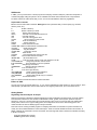
Next, prepare a code book with details of the data layout. Following is a code book for your research. Preparing a
code book would be helpful for researchers of all levels.
VARIABLE NAME WIDTH COLUMNS VALUE LABELS
ID
2 1-2
GENDER
1 3
M=male, F=female
LEVEL
1 4
1=1 yr or less,2=2 yrs,3=3 yrs
AREA
1 5
1=rural,2=city,3=suburban
V1
1 6
1=s.agree, 2=agree, 3=undecided,
4=disagree, 5=s.disag.
V2
1 7
"
V3
1 8
"
V4
1 9
"
V5
1 10
"
V6
1 11
"
V7
1 12
"
V8
1 13
"
V9
1 14
"
V10
1 15
"
S1
1 16
"
S2
1 17
"
S3
1 18
"
S4
1 19
"
S5
1 20
"
S6
1 21
"
S7
1 22
"
S8
1 23
"
S9
1 24
"
S10
1 25
"
MATH
2 26-27
COMP
2 28-29
In this code book, VARIABLE NAME stands for the name of the variable in the data, and WIDTH stands for the
number of fields taken by each variable. For example, the variable ID takes a maximum of two fields/columns, since
the highest ID number is 40. Similarly, EXP takes a maximum of one column/field. COLUMNS stands for the column
number/s on a given line where SPSS can find a value for each variable. VALUE LABELS means the value
represented within a variable. For example, within the variable SEX, M represents male and F represents female
students. Within the variable SCHOOL, 1,2,3 represent rural, city, and suburban schools, respectively.
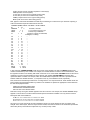
Now, examine how the data layout will look on a coding sheet or on a computer terminal. These variable values are
being copied from questionnaires filled in by students. The variables are placed into appropriate columns based on
the code book prepared earlier.
01M12123112245222113541213944
02F22325445211233445422212526
03F11211551141121122155114845
Note that on every line a given variable appears in the same column/s. For example, the variable GENDER always
appears in column three. In the above data no blank space is left between variables. You may choose to leave a
blank space after each variable as:
01 M 1 2 1 2 3 1 1 2 2 4 5 2 2 2 1 1 3 5 4 1 2 1 39 44
02 F 2 2 3 2 5 4 4 5 2 1 1 2 3 3 4 4 5 4 2 2 2 1 25 26
03 F 1 1 2 1 1 5 5 1 1 4 1 1 2 1 1 2 2 1 5 5 1 1 48 45
As long as you convey the format correctly to SPSS, the format you choose should not have any impact on the
analysis. In the above layout, there are only three lines of data, and each line stands for an observation (information
about each person). Note that each subject has only one line (record) of data.
Using an editor such as vi or pico, you can enter the data directly into your account on a UNIX-based system. Or, you
can type the data using a microcomputer text editor and save it on a floppy diskette for transfer to a UNIX platform
using FTP (File Transfer Protocol) or any other appropriate communication package.
Basic elements of an SPSS syntax file
The SPSS program consists of commands for defining and analyzing your data. In an SPSS program file, there are
two distinct parts: (1) data definition and (2) procedure section.
1. Defining data
In the data definition section, the variables involved in the study are specified, followed by the locations/columns in
which they're entered. This includes the number of columns occupied by each variable, decimal points, if appropriate,
and the type of variable (numeric or string). The data definition section may also contain information on specification
of missing values for the data set, variable labels, and value labels for the variables involved. Finally, a data definition
section can contain a number of data transformation/manipulation commands to organize the data before analysis.
All SPSS commands must begin in column one and continue on for as many lines as needed. Command lines that
continue on more than one line must be indented at least one column for continuation lines. Each command should
end with a period, which serves as the line termination character, although it is not required when running SPSS in
batch or non-interactive modes. A period at the end of each command is always required in DOS, Windows, and
Macintosh versions of SPSS, so it is a good practice to always use a command terminator, regardless of operating
system.
The SPSS commands are not case sensitive, but it preserves upper and lower case within labels and strings. SPSS
also distinguishes between an uppercase and lowercase character within a string variable. For example, in a variable
gender the value F is not the same as the value f. Unix is case sensitive, however, education.dat and
EDUCATION.DAT are different filenames in Unix.
Each command begins with a keyword, followed by command specifications. Keyword and specifications are
separated by at least one space.
TITLE command
The first line of an SPSS program may be a TITLE command. This command gives a title for your study and prints it
at the top of every page of output. The SUBTITLE command gives subtitles for your analysis. Both of these
commands can be up to 60 characters long. You can insert as many of these commands as you wish into your
program, but don't place them between a procedure command and BEGIN DATA when the data are inline, or within
the data records. Each command overrides the previous one. However, these two commands are optional.
TITLE 'Marketing Strategies'.
SUBTITLE 'Frequency analysis'.
DATA LIST command
A typical SPSS program may start with a DATA LIST command, followed by FILE definition (if data are not inline),
variable names, and column locations.
DATA LIST FILE = 'pathname/filename'
/ var1 col# var2 col# ... varn col#.
The DATA LIST command tells SPSS to prepare to read some data. The FILE definition portion of the data list points
SPSS to the data file, and indicates the format of the file. The pathname shows the directory in which the data file
resides. Replace pathname with an appropriate directory name and filename with the name of the data file. If the
data file is in the default directory, a pathname is not necessary. In this document we assume the data file is stored in
the same directory along with the command file. If your data contains multiple lines per case (observation), indicate
that along with the file definition.
DATA LIST FILE=education.dat FIXED RECORDS=2
/1 id 1-2 gender 3 (A) test1 10-11 test2 25-26
/2 final 1-4 (2) iq 8-10.
In the above command line, the keyword FIXED indicates that the data are presented in fixed format. That is, each
variable is recorded in the same location on the same record for each case. FREE and LIST are other two format
types. In FIXED format, a fortran-like format specification is also permitted.
DATA LIST FILE=clas.dat FIXED RECORDS=2
/1 id gender test1 test2 (F2.0,A,6X,F2.0,13X,F2.0)
/2 final iq (F4.2,3X,F3.0).
The RECORDS subcommand specifies the number of records (lines) per observation. This subcommand is not used
with free or list formats. In the above example the variable id is in columns 1-2 on the first record of each observation.
The variable sex is alphanumeric (character), as indicated by (A), and is in column 3 of the first record. The DATA
LIST command, by default, assumes all the variables are numeric. If a variable is alphanumeric, you need to define it.
If an alphanumeric variable has 2 characters, specify it as (A2), 3 characters as (A3), and so on. The variable final is
in columns 1-4, and the variable iq is in columns 8-10, both on the second record. By default, DATA LIST assumes
that the data are whole numbers or that decimal points have been recorded on the data file. To indicate non-integer
values when a decimal point is not actually coded in the data, specify the number of implied decimal places in
parentheses following the column specification. In the above example, the variable final is in columns 1-4, but the
last 2 digits are decimal points. Since this decimal point was not included when the data were entered, you indicate
this in the format statement.
MISSING VALUE command
There are several options to indicate missing values in a data file. You can leave missing values blank or code them
with a specification of your choice. When you leave a field blank SPSS by default assigns a system-missing value to
that field. If you decide to leave a blank for missing values, a MISSING VALUE command is not required in the
program file. However, some researchers choose to assign unique values for missing data (e.g. 9, 99, 0).
MISSING VALUES salary (99) age (9).
In the above example, missing values for salary and age are coded as 99 and 9, respectively.
VARIABLE LABLES command
The VARIABLE LABELS command in SPSS is used to assign an extended descriptive label to variables. Specify the
variable name followed by a blank and the associated label enclosed in apostrophes or quotation marks. Each
variable label can be up to 120 characters long, but most procedures print fewer than 120 characters for each label in
the output.
VARIABLE LABELS salary 'current salary for the employee'
exp 'years of experience with the present employer'
age 'present age'.
VALUE LABELS command
The VALUE LABELS command is used to assign labels to the values of variables. The value labels command is
followed by a variable name, or variable list, and a list of values with the associated labels. Value labels can have a
maximum of 60 characters; however, most procedures print out fewer characters for each label.
VALUE LABELS age 1 '20-29 yrs' 2 '30-35 yrs' 3 '36-41 yrs'
4 '42+ yrs' / sex 'M' 'male' 'F' 'female'.
Reading inline data
Earlier in this section, you used the FILE command to indicate the name of the file where the data is stored. If your
data are inline, omit the FILE subcommand on the DATA LIST command. You'll need two SPSS commands to
separate lines containing data from lines containing SPSS commands: BEGIN DATA and END DATA.
TITLE 'employee grievances study'.
DATA LIST
/ id 1-2 sex 3 (A) salary 5-11 (2) position 15 age 18-19.
VARIABLE LABELS id 'identification number' salary 'current salary'
position 'job classification' age 'present age'.
VALUE LABELS sex 'M' 'male' 'F' 'female'/
position 1 'managerial' 2 'professional' 3 'clerical'.
MISSING VALUES salary (999) position (0).
BEGIN DATA
01M 1838235 1 23
02F 2145325 1 31
03M 2382329 2 29
04F 126825 3 27
END DATA.
SPSS allows you to create and refer to a set of variable names by using the keyword TO. Suppose you have 20
items for a questionnaire in your study. When you are assigning names, item1 TO item25 is equivalent to 25 names:
item1, item2, item3, .... item24, item25. The prefix can be any valid name and the numbers can be any integers as
long as the first number is smaller than the second, and the full variable name, including the number, does not
exceed 8 characters.
DATA LIST FILE=dstudy.dat RECORDS=3
/1 id 1-3 qn1 TO qn25 4-28
/2 item1 TO item50 1-50
/3 ascale1 TO ascale5 1-10.
Note that on record 3 there are 5 variables with a total of 10 columns. SPSS automatically divides the 10 columns
equally among the 5 variables. You can also use the keyword TO in a number of command lines (e.g., VALUE
LABELS, RECODE, FREQUENCIES).
RECODE and COMPUTE commands
The ability to transform data is another important feature of SPSS. Two commands that form the core of the
transformation language are RECODE and COMPUTE. The RECODE command is used to change the coding
scheme of an existing variable on a value by value basis or for ranges of values. To recode the values of item3,
item9, and item21 from 5, 4, 2, and 1 to 1, 2, 4, and 5, use the command below:
RECODE item3 item9 item21 (5=1) (4=2) (2=4) (1=5).
There are a number of keywords that could be used with the recode command.
RECODE age (LO THRU 20=1).
RECODE age (LO THRU 20=1) (ELSE=2).
RECODE item1 TO item4 (0=1) (1,2=0) (ELSE=SYSMIS).
RECODE age (MISSING=9) (18 THRU HI=1) (0 THRU 18=0) INTO voter.
RECODE state ('MI'='MN').
The COMPUTE command is used to create a new variable or transform an existing one using information from other
variables in your file. The COMPUTE command generates a variable on your active file on a case-by-case basis. To
compute a variable specify the target variable on the left of the equals sign and the expression on the right.
COMPUTE subscore=item1+item2+item3+item4+item5.
There are several functions (e.g., arithmetic, statistical, logical) that can be used with the compute command.
COMPUTE subscore=SUM(item1 TO item5).
COMPUTE x=y*5.68.
COMPUTE pctwages=(wages/income)*100.
COMPUTE allavg=MEAN(qn1 to qn25).
COMPUTE m=SQRT(x1).
SELECT IF command
SPSS allows you to control the number and groups of cases used in analysis by selecting the observations you
specify with the SELECT IF command. These selections can be either temporary or permanent.
SELECT IF (sex EQ 'M').
This command selects cases for which the variable sex has the value M. The SELECT IF command permanently
selects cases, unless it's preceded by the temporary command.
TEMPORARY.
SELECT IF (sex EQ 'M').
FREQUENCIES VARIABLES=salary age.
In this case, the temporary selection of male population ends as soon as the FREQUENCIES procedure is executed.
You may also use SELECT IF to set multiple conditions. Suppose you want to permanently select, for further
analysis, all the males over 40 years of age. You may issue following the command:
SELECT IF sex EQ 'M' AND AGE GE 40.
There are a number of logical (e.g., AND, OR, ANY) and relational operators (e.g., EQ, NE, GT, LT, GE) you can use
for data transformation.
COMMENT command
Comments can help you and others review what you intend to accomplish with individual commands and blocks of
commands. SPSS ignores the comment part when it runs a job. You can insert comments using the COMMENT
command or an asterisk (*), or by enclosing the comment within /* and */ in any command line.
COMMENT select all the males from the data.
Comment can also be inserted with an asterisk (*), as in:
* select all the cases with values 1 or 2 for the variable income.
You may also use the comment within /* and */.
/* three categories are to be created */
Another reasonable place for the comment is at the end of the line, in which case the closing is optional, as in:
RECODE income (2,3=1) (else=1). /* recoding the values for income */
2. Data analysis
SPSS has a variety of procedures for statistical analysis you can choose based on your needs, e.g., FREQUENCIES,
DESCRIPTIVES, CROSSTABS, CORRELATIONS, ANOVA, MANOVA, and REGRESSION. Below are some brief
examples with samples of the output these commands generate.
Note: the data used in this section are described above. The actual program file is in the next section titled "Writing
an SPSS program."
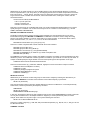
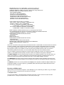
CORRELATION command
The procedure CORRELATIONS produces Pearson product-moment correlations with significance levels and,
optionally, univariate statistics, covariance, and cross-product deviations. For example, to correlate a single variable
against three other variables, you would use the following syntax:
CORRELATIONS VARIABLES=compopi WITH mathatti mathscor compscor.
The following correlation matrix is produced:
- - Correlation Coefficients - MATHATTI MATHSCOR COMPSCOR
COMPOPI
.2589
.1743
.7719
( 40) ( 37) ( 38)
P= .107 P= .302 P= .000
(Coefficient / (Cases) / 2-tailed Significance)
" . " is printed if a coefficient cannot be computed
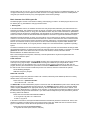
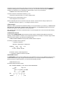
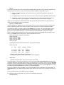
CROSSTABS command
The CROSSTABS procedure produces tables that are joint distributions of two or more variables that have a limited
number of distinct values. Again, using the data described above, if you wanted a breakdown of the students by
gender and years of computer experience, you would use the following command:
CROSSTABS sex by exp.
The following table presents the results:
SEX STUDENT GENDER by EXP YRS OF COMP EXPERIENCE
EXP
Page 1 of 1
Count |
|UPTO 1 Y 2 YEARS 3 OR MOR
|R
E
Row
| 1 | 2 | 3 | Total
SEX
--------+--------+--------+--------+
F | 7 | 7 | 8 | 22
FEMALE
|
|
|
| 55.0
+--------+--------+--------+
M | 8 | 7 | 3 | 18
MALE
|
|
|
| 45.0
+--------+--------+--------+
Column
15
14
11
40
Total 37.5 35.0 27.5 100.0
Number of Missing Observations: 2
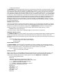
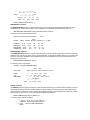
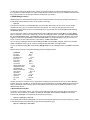
DESCRIPTIVE command
The DESCRIPTIVES procedure computes univariate summary statistics and standardized variables. Using the
sample data, you could produce a table of basic statistics on four variables with the following command:
DESCRIPTIVES VARIABLES=compopi mathati mathscor compscor.
The output for this command appears below:
Number of valid observations (listwise) =
Variable
Mean
35.00
Valid
Std Dev Minimum Maximum
COMPOPI
27.93
11.53
MATHATTI 38.83
12.55
MATHSCOR 40.65
7.57
COMPSCOR 35.95
6.57
13
15
20
24
N Label
46 40
50 40
50 37
48 38
FREQUENCIES command
The FREQUENCIES procedure computes a table of frequency counts and percentages for the values of individual
variables. This command is typically used to get the breakdown of categorical variables. Below is an example of the
syntax for obtaining a distribution of the variable SCHOOL which indicates the type of school the students in the
sample data set come from.
FREQUENCIES VARIABLES = school.
The following output is generated:
SCHOOL
SCHOOL REPRESENTING
Value Label
RURAL
CITY
SUBURBAN
Valid Cum
Value Frequency Percent Percent Percent
1
13 31.0 32.5
32.5
13 31.0 32.5
65.0
3
14 33.3 35.0 100.0
.
2
4.8 Missing
------- ------- ------Total
42 100.0 100.0
2
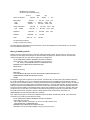
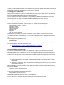
ANOVA command
The ANOVA procedure performs analysis of variance for factorial designs. The example below attempts to test the
relationship between gender and computer experience, again drawing from the sample files. Notice that the SEX
variable has been recoded into a new variable called NSEX because the original variable was a character variable
which cannot be used in many of the more sophistical statistical procedures.
ANOVA COMPOPI BY EXP (1,3) NSEX (1,2).
A summary of the results is as follows:
*** ANALYSIS OF VARIANCE ***
COMPOPI TOTAL FOR COMP SURVEY
by EXP
YRS OF COMP EXPERIENCE
NSEX
UNIQUE sums of squares
All effects entered simultaneously
Source of Variation
Main Effects
EXP
NSEX
Sum of
Squares
Mean
DF
Sig
Square
of F
742.012
3
247.337 2.176 .109
566.882
2
283.441 2.493 .098
340.840
1
340.840 2.998 .092
2-Way Interactions
EXP
NSEX
903.184
903.184
2
2
451.592 3.972 .028
451.592 3.972 .028
Explained
1319.489
5
263.898
Residual
3865.286
34
113.685
Total
F
5184.775
39
2.321 .064
132.943
42 cases were processed.
2 cases (4.8 pct) were missing.
For further details on data definitions and procedures, see the SPSS Reference Guide (Release 6.1), and SPSS
Advanced Statistics (Release 6.1).
Writing an SPSS syntax file
Now that we have looked at the steps involved in creating an SPSS program, the next step is to write one.This
example is for the sample research topic we discussed earlier. Suppose you decided to include your data within
(inline) the program file. First, look at the program file in its simple form.
TITLE 'COMPUTER ANXIETY IN MIDDLE SCHOOL CHILDREN'.
DATA LIST /ID 1-2 SEX 3 (A) EXP 4 SCHOOL 5 C1 TO C10 6-15
M1 TO M10 16-25 MATHSCOR 26-27 COMPSCOR 28-29.
MISSING VALUES MATHSCOR COMPSCOR (99).
BEGIN DATA
[data entered here]
END DATA.
LIST VARIABLES=SEX EXP SCHOOL MATHSCOR COMPSCOR/CASES=10.
FREQUENCIES VARIABLES=SEX EXP SCHOOL.
FINISH.
The program begins with an optional TITLE command. The DATA LIST command names the variables followed by
the column specification for each. The TO keyword specifies the names of variables in sequential order. Missing
values for the two variables (mathscor, compscor) are declared through the MISSING VALUE command. A comment
is added to the end of the missing value command demarcated by /*. Since the data are inline, the beginning of the
data line is declared using the BEGIN DATA command, and the end of the data line with the END DATA command.
The LIST procedure displays in standard format the values of the variables for 10 cases in the active file. Using this
procedure may be a good way to check whether the data are being read by program as you wanted them to read.
The CASE subcommand controls the number of observations to be processed for this procedure. The
FREQUENCIES command requests tables for 5 variables.
Next, expand the program to include some additional features of SPSS. The data file, clas.dat, is an external file.
Comments are provided in several places for clarity.
TITLE 'COMPUTER ANXIETY IN MIDDLE SCHOOL CHILDREN'.
DATA LIST FILE=clas.dat
/ID 1-2 SEX 3 (A) EXP 4 SCHOOL 5 C1 TO C10 6-15 M1 TO M10 16-25
MATHSCOR 26-27 COMPSCOR 28-29.
MISSING VALUES MATHSCOR COMPSCOR (99).
RECODE C3 C5 C6 C10 M3 M7 M8 M9 (1=5) (2=4) (3=3) (4=2) (5=1).
RECODE SEX ('M'=1) ('F'=2) INTO NSEX. /* char var into numeric var
COMPUTE MATHATTI = M1+M2+M3+M4+M5+M6+M7+M8+M9+M10.
COMPUTE COMPOPI = SUM (C1 TO C10) /* total 10 items using SUM function
VARIABLE LABELS ID 'STUDENT IDENTIFICATION'
SEX 'STUDENT GENDER'
EXP 'YRS OF COMP EXPERIENCE'
SCHOOL 'SCHOOL REPRESENTING'
MATHSCOR 'SCORE IN MATHEMATICS'
COMPSCOR 'SCORE IN COMPUTER SCIENCE'
COMPOPI 'TOTAL FOR COMP SURVEY'
MATHATTI 'TOTAL FOR MATHATTI SCALE'.
VALUE LABELS SEX 'M' 'MALE' 'F' 'FEMALE'/
EXP 1 'UPTO 1 YEAR' 2 '2 YEARS' 3 '3 OR MORE YRS'/
SCHOOL 1 'RURAL' 2 'CITY' 3 'SUBURBAN'/
C1 TO C10 1 'STRONGLY DISAGREE' 2 'DISAGREE'
3 'UNDECIDED' 4 'AGREE' 5 'STRONGLY AGREE'/
M1 TO M10 1 'STRONGLY DISAGREE' 2 'DISAGREE'
3 'UNDECIDED' 4 'AGREE' 5 'STRONGLY AGREE'.
PRINT FORMATS COMPOPI MATHATTI (F2.0). /*Specifying the print format
LIST VARIABLES=SEX EXP SCHOOL MATHSCOR COMPSCOR COMPOPI MATHATTI
/FORMAT=NUMBERED/ CASES=10. /* only the 1st 10 cases
FREQUENCIES VARIABLES=SEX,EXP,SCHOOL
/STATISTICS=ALL.
TEMPORARY.
SELECT IF SEX EQ 'F'.
FREQUENCIES VARIABLES=SEX EXP SCHOOL
/STATISTICS=ALL.
CROSSTABS TABLES=SEX BY EXP SCHOOL.
DESCRIPTIVES COMPOPI MATHATTI MATHSCOR COMPSCOR.
ANOVA COMPOPI BY EXP (1,3) NSEX (1,2).
FINISH.
Some of the commands in this program may need further discussion. The RECODE command reverses the values of
a number of variables. It also changed the variable sex to a numeric variable named nsex. SPSS does not permit
you to change a variable from string to numeric or from numeric to string by recoding it into itself. You can use the
INTO keyword to specify a new variable in recode command. String variables cannot be used on a number of
mathematical operations and functions. The new variable, nsex, is later used in the ANOVA procedure.
Two new variables (compopi and mathatti) are created using the COMPUTE command. Two methods, arithmetic
operator (+) and statistical function (SUM), are used to create new variables for the purpose of illustration.
The PRINT FORMATS command changes the print formats for the variables specified on the command. When you
create a new variable (e.g., compopi, mathatti) using the transformation language, the default format is F8.2. To
override this feature and to get the value printed as you want, use the PRINT FORMAT command.
The TEMPORARY command is used to create a temporary data set with the female population alone and to run a
frequency analysis with selected variables. Once the frequency procedure is executed the temporary transformation
ends.
The ANOVA procedure runs a two-way ANOVA with compopi as the dependent variable and exp and nsex as the
independent variables. A number of options (e.g., MISSING, REG, STATISTICS) are available with this and other
procedures used in the program.
Executing an SPSS program
Suppose that you saved the above program in a file, clas1.sps, in your root directory (to obtain a copy, see "Sample
Files" above). There are several ways to execute these commands.
1. Prompted session
You may access SPSS in a prompted session (interactive line mode). You don't need an X terminal to start a
prompted session. To begin a prompted session, at the system prompt, type:
spss -m
In the above command, m is one of several switches available with SPSS under Unix. Them switch suppresses the
Manager mode or the Window mode. A few of the other switches available in SPSS under Unix are:



t output -- to send the listing file to the terminal and to a file simultaneously. Replace output with an
appropriate name.
p -- displays output on the terminal one screen at a time. This is the same as the more command in Unix.
s workspace -- replace workspace with the number of bytes to be used for working storage. Specify a
number followed by k () or m (megabytes). The default is 512K. This is sufficient for most jobs.
Suppose you want to start a prompted SPSS session with the output file stored as test.lst, and want to view the
output on a terminal page by page. You would type:
spss -m -p -s 300k -t test.lst
Command switches are applicable for any mode of SPSS access. You must specify them when you invoke SPSS.
See the SPSS Base System Users's Guide for UNIX for further information on switches available with SPSS.
Once SPSS is invoked, you will see the SPSS prompt SPSS> at the input line. This means that SPSS is ready to
accept your input commands. Each SPSS command is terminated by a period (.). A command, starting with a
keyword, may span across several lines. A command terminator informs SPSS that a command is complete.
Below is a sample SPSS prompted session. Start your prompted session by typing spss -m at the system prompt.
When you see SPSS> type the following lines, pressing ENTER after each line.
SPSS> data list free / id age educ exper salary.
SPSS> begin data
DATA> 01 32 16 4 32000
DATA> 02 24 13 2 19000
DATA> 03 42 18 8 41000
DATA> end data.
Preceding task required .02 seconds CPU time; 105.32 seconds elapsed.
SPSS> list var=all.
ID
AGE
1.00 32.00
2.00 24.00
3.00 42.00
EDUC
16.00
13.00
18.00
EXPER
4.00
2.00
8.00
SALARY
32000.00
19000.00
41000.00
Number of cases read: 3 Number of cases listed: 3
Preceding task required .01 seconds CPU time; .12 seconds elapsed.
SPSS> finish.
End of job: 8 command lines 0 errors 0 warnings 0 CPU seconds
In the above session, you typed in the data lines. You may also use the data list file=myfile.dat command to read
an external data file into a prompted session. During a prompted session, you have the option of using the INCLUDE
command t o read in a stored command file. If you decide to type in the command lines, you can save the commands
you type in a journal file for later use. To turn the journaling on, at the SPSS> prompt, type set journal.You can stop
journaling by typing s et journal off, and resume it by typing set journal on.
For help, at the SPSS> prompt, type help. You may also type help to receive a description of the help facilities, or
help keyword (where you replace "keyword" with by anova, manova, t-test, report, etc.) to get help on the topic yo u
want.
To end a prompted session, at the SPSS> prompt, type finish.
If you decide to read in a command file, e.g., clas1.sps, at the SPSS> prompt, type:
include clas1.sps
The file will be read into the SPSS session and the commands executed. The listing will be displayed on the screen.
If you specified an output filename, the output would be stored in that file. Note: if you have a FINISH command in the
file you are rea ding in from a prompted session,it will terminate your session.
2. SPSS Manager session
SPSS Manager is a character-based interactive interface designed to help you build and run SPSS commands. To
invoke SPSS under a Manager session, at the system prompt, type:
spss +m
This opens two windows in the SPSS Manager: the Input window at the bottom of your screen, and the Output
window at the top. Type your command lines in the Input window. To run the job, first move the cursor to the
beginning of the line where the execu tion should begin, then open the run menu by pressing Esc 0 and selecting
run from the cursor.
You can also read in a file you already created and saved into a Manager session (press Esc 3 and select Insert
file). For example, to read in the command file, clas.sps, at the Manager session, press Esc 3, then select Insert f
ile. At the File to Insert prompt:, type clas1.sps. Now the file will be included in the window. Move the cursor to the
beginning of the file and press Esc 0 and select run from cursor. The output will appear in the top por tion of the
screen. To move into the Output window or Input window, use Esc 2 and switch.
You can also run a Manager session in Menu Mode (press Esc 1 and select M). The Menu mode has an interface
similar to SPSS/PC+ where you can select the commands and paste them to the Input window.
You can get help by pressing Esc 1 and selecting manager help. To exit a Manager session, press Esc 0 and select
exit.
Below is a brief summary of the keyboard mapping during a Manager session:
Command
run menu
information
windows menu
files menu
lines menu
look menu
go to menu
mark/unmark menu
marked area menu
write/delete file
switch Input/Output
menu mode
edit mode
switch mode
menu off
top menu
exit
Key
Esc 0
Esc 1
Esc 2
Esc 3
Esc 4
Esc 5
Esc 6
Esc 7
Esc 8
Esc 9
Esc S
Esc 1 M
Esc E
Esc S
Esc M
Esc Esc
Esc 0 E
Use the arrow keys to move the cursor in any window. Not all keys become active as soon as you start a Manager
session. Some work only after you incorporate lines into the Input Window. For example, Esc 8 becomes active only
after you press E sc 7 and mark lines. See the SPSS Base System User's Guide for UNIX for information on the
SPSS Manager session.
3. Non-interactive session
To initiate a non-interactive session, you need a command file saved with all the necessary SPSS commands you
want to use. In this instance, we created a command file, clas1.sps, with its data file, clas.dat. To execute the
command file, clas1.sps, non-interactively, at the system prompt, type:
spss -m < clas1.sps > clas1.out
The output file will be stored as clas1.out. You cannot use the terminal while the job is running. However, if you want
to free the terminal for other work while the job runs in the background, type:
spss -m < clas1.sps > clas1.out &
You will see a process identification number (PID) for the background task and your terminal will be free for other
computing. To check the status of the job, at the system prompt, type the ps command. Once the job is executed, the
listing file will be stored in the default directory or in the directory you specify.
4. Sending jobs to a batch queue
Batch queues are available on the SP. You must submit CPU-intensive jobs to the batch queue for execution. Jobs
that exceed the limits described below will be terminated automatically.
There is a special queuing system on Research SP (e.g., aries05) for submitting long SPSS jobs to run in batch
mode. CPU-intensive jobs (requiring more than 20 minutes of CPU time) must be submitted to IBM's LoadLeveler
batch queuing system. Two types of queues are available for statistical jobs on aries05. They are:
stat
jobs requiring up to 8-day of CPU time
To submit an SPSS job to LoadLeveler, create a script file, e.g., spsjob1, with the following lines:
#@ requirements = (Feature == "spss")
#@ group = standard
#@ initialdir = directory
#@ error = filename
#@ class = stat
#@ queue
spss -m < inputfile > outputfile
Replace directory with the directory where the command file is stored. Replace filename with a name for the
LoadLeveler error/log file which will be stored in the same directory. Replace inputfile (e.g., clas1.sps) with the name
of the SPSS command file, and outputfile (e.g., clas1.out) with an appropriate name for storing the output from the
run.
To submit the job, at the system prompt, type:
llsubmit spsjob1
The output files will be stored in the directory you specified in the script file. You may log out after submitting the job.
For more information on batch jobs on SP System, visit:

The UITS Research SP System - Submitting Batch Jobs to LoadLeveler
Accessing SPSS from an X-terminal
If you want to use all the features of SPSS for Unix (Release 5.0 or higher), you must access it from a Unix Xwindows environment. One of the most attractive features of the latest versions of SPSS is the Motif graphical users
interface (GUI), which makes it easier to learn and use. This provides descriptive menus and simple dialog boxes
providing a point-and-click environment for SPSS that is very similar to the Windows and Macintosh versions. The
Motif interface also provides several other features:



Data Editor. A versatile spreadsheet-like system for defining, entering, editing, and displaying data.
High-resolution graphics. High-resolution, full-color charts and graphics as a standard feature in SPSS
Base system.
Chart Editor. A highly visual, object-oriented facility for manipulating and customizing the many charts and
graphs produced by SPSS.
Before invoking SPSS, set up the terminal for proper display. Korn or Bourne shell users should add the following
lines into the .profile file.
DISPLAY = nnn.nnnn.nnnn.nnnn:0;export
DISPLAY
C shell users should add the following line to the .login file.
setenv DISPLAY nnn.nnn.nnnn.nnn:0
Replace nnn.nnn.nnnn.nnn with the IP number of your workstation.
To access SPSS from a windowing environment, at the system prompt (in X-windows), type:
spss
If you want to use the same X window for other tasks, type:
spss &
The first time you start an SPSS session, the Startup Preferences dialog box opens. To accept the default settings,
click OK. This opens three other windows: output window, syntax window, and data editor window. At this point, you
can open an existing SPSS system file, or define new data files through menus. You can accomplish most of the
tasks by simply pointing and clicking the mouse.You can define the colors for your windows through -bd (border
color), -bg (background color), and -fg (foreground color). For example, the command below will start a session with
the specified colors for the windows.
spss -bd red -bg cyan -fg black $
You can also define an alias in your .kshrc or .cshrc for running SPSS. The default workspace during a Motif session
is 1512K.
To read your command file, clas1.sps, into an SPSS Motif session, select FILE-> Open -> SPSS Syntax. To execute
the job, click the "run" button (the second button from the right, on the button bar). The output will be stored in the
output window. To exit the session, select FILE -> EXIT from any of the windows. Note that an SPSS Motif session is
very similar to an SPSS for Windows session.
For help on a specific topic during an SPSS Motif session, click the menu bar Help option. You may also click the
Help pushbutton in an SPSS dialog box. Another option is to press F1 at any time and select the topic you want.
Finally, for specialized help, click the Glossary pushbutton in an SPSS output window or the Syntax pushbutton in a
syntax window. For an overview of how to use the help system, select On Help from the Help menu.
For more on an SPSS Motif session, see SPSS Base System User's Guide for UNIX.
Printing files from Unix systems
lpr -Pprintername filename
Replace printername with the name of any of the UITS supported printers, and filename with the name of the file
you want to print. You may download a file to your workstation and print it on your printer. Contact a UITS consultant
if you need help.
SPSS Data Sets
SPSS system files
A system file is a file that contains data and program together in binary format. These files can be processed by
computers much more quickly than can ASCII files. Creating a system file substantially reduces the computer
processing time, especially with several data transformation steps. System files are normally created with variable
names, value labels, variable labels, and data manipulation steps.
Suppose you want to create a system file from the data (clas.dat) and command (clas1.sps) files created earlier. Add
the SAVE OUTFILE immediately after the VALUE LABELS command in the command file.
The general syntax for creating a system file is:
SAVE OUTFILE='systemfile'.
Replace systemfile with an appropriate path name and filename for storing the system file. Note: Any external file in
SPSS that is encased in single-quotes must be in the correct case.
A system file is readable only by the operating system from where it was created. The general syntax for accessing a
system file is:
GET FILE='systemfile'.
Replace systemfile with the name of the file. Specify a full pathname when applicable.
SPSS portable files
If you are using SPSS under other operating systems (e.g., Macintosh, Windows), you can move your SPSS files to a
Unix environment. However, SPSS system files created under one operating system are not readable under another
system. For example, an SPSS system file created under Windows is not readable under Unix. There are variations
of Unix, and system files created under one Unix platform are not readable from anoth er. For example, a SPSS
system file created under SunOS (Steel) is not readable under IBM AIX (SP), and vice versa.
When you want to use a system file created under one operating system on another, you must create an export file
and move it to the host machine. The general syntax (irrespective of the operating system) for creating an export
format file is:
EXPORT OUTFILE='exportfile'.
Replace exportfile with appropriate filename. In some instances, you may want to give the full pathname where the
export file is to be stored. Once the export file is in the designated operating system, use the import command to
read the import file. The general syntax for reading an export file is:
IMPORT FILE='exportfile'.
Replace exportfile with the name of the file you moved from the source operating system.
If you want to create a system file from the export file, add another command line to the above import command line:
SAVE OUTFILE='systemfile'.
Replace systemfile with an appropriate filename for storing the system file.
Reading compressed files
For SPSS 6.1 on UNIX, you can create and use compressed ASCII data files, SPSS systems files, and SPSS
portable files. This means you can compress any SPSS data files you have in order save disk space on your account.
To compress an SPSS file, use the UNIX "compress" command which uses the Lempel-Ziv compression method. At
your UNIX prompt, type:
compress filename
Replace the filename with the name of the file you want to compress. This creates a new file with the extension ".Z".
For example, if you compressed a file called "test.dat," a compressed file called "test.dat.Z" would be created.
To read this file into SPSS, use the FILE HANDLE command. For example,
FILE HANDLE alias/INPIPE="zcat filename.Z".
Replace alias with the file handle (nickname) you'll assign the compressed file. It can be up to 8 characters long.
Replace filename.Z with the name of your compressed file (remember to always have a .Z extension). This can
either be an ASCII data file or an SPSS systems file. Be sure, also, to include the path of the data file if the file is
stored somewhere other than the default directory from which you are running SPSS.
For example, if you had an ASCII data file called "test.dat" with 10 variables (v1-v10) that you wished to compress
and then access, the command to compress the file is:
compress test.dat
To use this file in SPSS, use the following SPSS commands:
FILE HANDLE test/inpipe="zcat test.dat.Z".
DATA LIST FILE = test / v1 to v10.
You can then execute this command file as you normally would.
If you are using a compressed SPSS systems file, you would use the same syntax, but you would use the GET FILE
command instead of a DATA LIST statement. If "test.dat" was an SPSS systems file instead of a compressed ASCII
file, you would replace the second line above with:
GET FILE = test.
Finally, if "test.dat" were a compressed SPSS portable file, you would use the IMPORT FILE command:
IMPORT FILE = test.
Transferring files between SPSS and SAS
SPSS can read SAS transport format files and create SPSS system files. The general syntax for reading a SAS
transport format file and creating an SPSS system file is:
GET SAS DATA='sastransportfile'.
SAVE OUTFILE='fromsas.sys'.
Replace sastransportfile with the name of the SAS transport format file, and fromsas.sys with an appropriate
filename to store the system file. An SPSS system file or export file is also readable during a SAS session.
SPSS can also read data files created using Lotus, Excel, dBase, and so on. Refer to the GET TRANSLATE
command in the SPSS System Syntax Reference Guide (Release 5.0 or 6.1).