Download Sunfleck User Manual - manuals.decagon.com

S
D
N
F
L
E
C
R
E
T
E
M
T
O
P
U
E
C
P e
M ullm ca
ad
g
e an on
in , W
U A
S
A
IO
T
C
N
U
F
8
7
K
N
2 PA
3 Su R
4 Au nfl
5 Au to ec
A
6 Co to PA k
7 Tim nti Su R
T
n
S h e u n
sa
8 in re se o fle
E g sh t us ck
sa m
ra le o
re m ple
se S ld
re ad ple
o en or
ho ad
av
r s
S or
ho ld
av era
en
se urs
re era g
d
t
re ad g e
e
era
sto ad
m re
se
in
ute
se
s
se t
nd
1
6
B
5
4
3
2
1
Sunfleck
PAR Ceptometer
1
10
20
30
40
50
60
70
Operator's Manual
Table of Contents
1. Introduction
About This Guide
Warranty
Customer Service Information
Seller's Liability
2. About the Sunfleck Ceptometer
3. Getting Started
Installing the Batteries
Calibration
Finding the Zenith Angle of the Sun
Direct Measurement
Calculation
Example Calculation
4. Keyboard Operation
Overview of Functions
Function 1: PAR Measurement
Function 2: Sunfleck Measurement
Function 3: Unattended PAR Measurement
Function 4: Unattended Sunfleck Measurement
Function 5: Continuous Sunfleck and PAR
Readings
Function 6: Setting the Time
Function 7: Setting the Threshold
Function 8: Send/Erase Memory and Individual
Sensor Dump
5. Measurement Tips
Discussion of the Effects of Non-Random
Distribution of Canopy Elements of LAI
Measurement in situ
6. Applications
PAR
Measuring Averaged and Intercepted PAR
Sampling for Fractional Interception
Unattended Recording of Transmitted PAR
Survey Sampling of Average Line PAR
Using PAR to Determine Leaf Area Index
Applications and Examples
Final Comments
Spectral and Cosine Response
2
4
4
4
4
5
6
9
9
10
11
11
13
14
16
16
19
20
21
22
22
23
24
26
27
28
31
31
31
33
36
37
37
41
42
42
7. Sunflecks
Setting the Threshold
Sampling for Sunfleck Fraction
Unattended Recording of Sunfleck Fraction
Survey Sampling of Sunfleck Fraction
8. The Theory of Sunflecks and Canopy Structure
Example
Computer Program to Find LAI and LAD
Correction of Sunfleck and Intercepted
Radiation for Sun Angle
Example
9. Interfacing with a Computer
Connections
BASIC Program
Notes on the BASIC Program
Executing the BASIC Program
Sunfleck SunView Software
Backing Up and Running SunView from
Floppy Disk
Installing SunView to the Hard Drive
Connecting the RS-232 Cable
Downloading Memory to a Computer
Running SunView Software
10. Maintenance
Changing the Batteries
Recalibrating the Sensors
Cleaning the Probe
11. Return and Repair
12. Questions and Answers
Appendix A: Additional Information
References
3
45
46
47
48
48
49
51
53
54
54
57
58
58
59
60
61
61
62
62
63
63
64
65
65
65
66
67
70
74
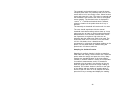
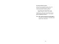
1. Introduction
The Sunfleck Ceptometer is a battery-operated PAR
sensor used for data collection in plant and forestry
canopy research. It will enable the user to collect and
store radiation data in the 400-700 nm PAR region.
The Ceptometer is easy to use and will give accurate
results when properly maintained.
About This Guide
Included in this manual are instructions for operation
and calibration of the Ceptometer along with
guidelines to help you maintain and care for your
instrument. Please read all of these instructions
before operating the Ceptometer to insure that the
instrument performs to its full potential.
Warranty
The Ceptometer has a 30 day satisfaction guarantee
and a one year warranty on parts and labor. To
validate your warranty, please complete and return
the warranty card included in this manual. It is
necessary for Decagon to have your current mailing
address and telephone number in case we need to
send updated product information to you.
Customer Service Information
If you ever have questions concerning the
Ceptometer or need assistance regarding your
instrument, please call our toll free customer service
number between 8 a.m. and 5 p.m. Monday through
Friday, Pacific Time.
1-800-755-2751
4
Seller's Liability
Seller warrants new equipment of its own manufacture
against defective workmanship and materials for a
period of one year from date of receipt of equipment
(the results of ordinary wear and tear, neglect, misuse,
accident, and excessive deterioration due to corrosion
from any cause not to be considered a defect); but
Seller's liability for defective parts shall in no event
exceed the furnishing of replacement parts f.o.b. the
factory where originally manufactured. Material and
equipment covered hereby which is not manufactured
by Seller shall not be liable to Buyer for loss, damage
or injuries to persons (including death), or to property
or things whatsoever kind (including, but not without
limitation, loss of anticipated profits), occasioned by or
arising out of the installation, operation, use, misuse,
nonuse, repair, or replacement of said material and
equipment, or out of the use of any method or
process for which the same may be employed. The
use of this equipment constitutes Buyer's acceptance
of the terms set forth in this warranty. There are no
understandings, representations, or warranties of any
kind, express, implied, statutory or otherwise
(including, but without limitation, the implied warranties
of merchantability and fitness for a particular purpose),
not expressly set forth herein.
5
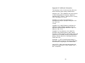
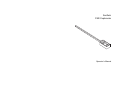
2. About the Ceptometer
The Sunfleck PAR Ceptometer is a battery-operated
PAR sensor used for data collection in plant and
forestry canopy research. Model SF-80 has 80
independent sensors located in a weather-proof
enclosure at one centimeter intervals along a sensor
probe. Model SF-40 has 40 sensors located in the
same manner. The datalogger is capable of either
hand-held push button operation or stand alone
measurements of light in plant canopies.
The sensors measure PAR (Photosynthetically Active
Radiation) in the 400 to 700 nanometer waveband.
Units of measurement for the instrument are µmol m2 -1
s .The Ceptometer has two main modes of
operation. In the first, the average photon flux density
of PAR on the probe is measured. In the second, the
fraction of the probe in sunflecks is measured and
reported. Other modes allow continuous display of
readings on a single sensor and stand alone data
collection in both modes.The datalogger averages
and stores measurements, and dumps them to a
computer when field measurements are complete.
The biggest problem with making reliable
measurements of light in plant canopies is the
extreme light level variation of the measurements. In
the PAR waveband, irradiances can vary from full sun
to almost zero over the space of a few centimeters,
and a reliable measurement of average PAR requires
many samples at many locations under the plant
canopy. The Ceptometer provides an easy way of
obtaining the necessary number of samples for light
measurement.
6
The instrument's 80 sensor probe is inserted into the
canopy, and a microprocessor scans the sensors. In
the sample mode, the Ceptometer displays a reading
( an average of the readings of all sensors) each time
the sample button is pushed, and the user discerns
when to average the accumulated readings and store
them in memory. In the auto mode, the unattended
Ceptometer takes readings every minute, then
averages and stores accumulated readings every 30
minutes.
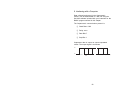
The Sunfleck application of the Ceptometer is an
added bonus. Sunflecks are the bright areas under
the canopy where direct beam solar radiation
penetrates without attenuation by the canopy. The
fraction of the ground covered by sunflecks is a useful
measurement for determining canopy cover. Sunfleck
fraction measurements can also be used with inverse
methods to determine important characteristics of
canopy structure. These will be discussed later in the
manual. Sampling, averaging, and auto mode
operation features for the sunfleck fraction mode are
similar to those in the PAR mode.
The Ceptometer can be operated in environments
0
0
with temperatures from -30 to 50 C, and relative
humidities up to 100%. The instrument comes with a
standard RS-232 interface cable for easy connection
to a user-provided computer. The Sunfleck provides
fast reading and averaging data, and stores over
1,000 data sets. Each stored data set includes time,
PAR, and sunfleck percentage regardless of the
operating mode.
Biomass production in plant communities is directly
related to PAR interception. The Ceptometer provides
the user with the measurements needed to interpret
field experiments.
7
Leaf area index and canopy cover can be estimated
from measurements of intercepted PAR. The
Ceptometer may also aid the user in understanding
the importance of sunflecks in the photosynthesis and
growth of forest understory plants and crops by
recording their occurrance. Other Ceptometer
applications include water stress studies, crop and
canopy modeling, plant disease and environmental
research, and fertilizer and pesticide efficacy studies.
8
3. Getting Started
There are a few things to consider before beginning
measurements with the Ceptometer. These consist of
installing the batteries, calibrating the instrument, and
finding the zenith angle of the sun.
Installing the Batteries
The Ceptometer's batteries are shipped separate of
the instrument and must be installed before
operation. To install the batteries, remove the four
screws in the corners of the instrument's cover and lift
the cover carefully. The battery clips will be visible as
the cover is lifted. Place the batteries in the battery
clips, making sure to orient them correctly as indicated
by the diagrams on the battery clip. Replace the cover
and the four screws.
Note: When shipping the Ceptometer, always remove
the batteries to prevent damage to the battery
clips.
When using the Ceptometer in the field, the
user may wish to download data to a portable
personal computer; rough terrain may cause
the batteries to shift and data may be lost.
9
Calibration
Each time the batteries are replaced or installed for
the first time, the Ceptometer's sensors must be
recalibrated. Calibration must be performed in bright,
even sunlight on a cloudless day. Shift to function
seven by pressing the function key until the display
pointer is stationed at function7. Hold down buttons A
and B simultaneously and press the function key. The
letter "PLL" will appear on the left side of the display.
This indicates that the probe has been correctly
calibrated. If these letters do not appear, refer to the
troubleshooting section of this manual.
Note: Be sure to recalibrate the Ceptometer in the H -mode of function seven and not the ELE
mode. If the ELE mode is used, the instrument
will not function properly and will need to be
recalibrated.
10
Finding the Zenith Angle of the Sun
Zenith angle of the sun is required for inversion of
canopy light transmission data to determine leaf area
index. Zenith angle can either be calculated from time
of day or measured directly. This section suggests
methods for finding the zenith angle of the sun.
Direct Measurement
The zenith angle is the angle the sun makes with
respect to a line vertical to the earth's surface. For
zenith angle, the point directly overhead would be
o
o
defined as 0 and the horizon defined as 90 . For
elevation angle, the point directly overhead would be
defined as 90o and the horizon 0o . The simplest
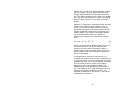
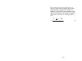
method for measuring zenith angle is to construct a
device as shown in Figure 1 from two pieces of wood
placed at right angles to each other. The top edge of
the vertical piece should be 10 centimeters above the
top surface of the horizontal piece, and the horizontal
piece should be 20 to 30 centimeters long. Mount a
bubble level and a ruler on the horizontal piece. To
measure zenith angle, level the horizontal piece with
the vertical piece perpendicular to the sun azimuth
and measure the length of the shadow on the
horizontal ruler. The zenith angle is calculated from
θ = arctan(x/10)
where x is the shadow length (cm) and 10 is the
height of the vertical piece.
11
10 cm
20
/30
cm
Figure 1. Board/Scale zenith angle device.
Another simple method is to attach a protractor to a
small board, mount a bubble level on the board to the
level of the protractor, and attach the end of a soda
straw with a pin to the center of the protractor so that
the straw can pivot across the face of the protractor.
To take a reading, level the board with the protractor
parallel with the sun azimuth, and adjust the soda
straw, watching its shadow on a surface below its end.
When light shines through the straw onto the surface,
read the angle from the protractor.
Figure 2. Protractor/Straw zenith angle device.
12
Calculation
The formulas for calculating elevation angle are
relatively straightforward. The zenith angle is
calculated from:
θ = arccos(sin L sin D + cos L cos D cos 0.2618(t-to))
(1)
where L is the latitude, D is the solar declination, t is
the time, and to is the time of solar noon. The earth
turns at a rate of 0.2618 radians per hour, so the
0.2618 factor converts hours to radians. Time, t, is in
hours (standard local time), ranging from 0 to 24.
Latitude of site is easily found in an atlas. Solar
declination ranges from +0.409 radians (+23.45
degrees) at summer solstice to -0.409 radians (-23.45
degrees) at winter solstice. It can be calculated from:
D = arcsin{0.39785 sin[4.869 + 0.0172 J + 0.03345
sin(6.224 + 0.0172 J)]}
(2)
where J is the day of the year. Some values are given
in Table 1. The time of solar noon is calculated from:
to = 12 - LC - ET
(3)
where LC is the longitude correction and ET is the
Equation of Time. LC is +4 minutes, or +1/15 hour for
each degree east of the standard meridian and -1/15
hour for each degree west of the standard meridian.
Standard meridians are at 0, 15, 30...345 degrees.
Generally, time zones run approximately +7.5 to -7.5
degrees either side of a standard meridian, but this
varies depending on political boundaries so check an
atlas to both standard meridian and longitude.
13
The Equation of Time is a 15 to 20 minute correction
which depends on the day of the year. It can be
calculated from:
ET = [-104.7sinφ + 596.2sin2φ + 4.3sin3φ - 12.7sin4φ
(4)
- 12.7sin4φ - 429.3cosφ - 2.0cos2φ +19.3cos3φ]/3600
where f = (279.575 + 0.986 J)p/180. Some values for
ET are given in Table 1.
Example Calculation
Find the zenith angle for Pullman, WA at 10:45 PDT
on June 30. Convert the time of observation to
standard time by subtracting one hour and convert
minutes to decimal hours, so t = 9.75 hours.
June 30 is J = 181.
Pullman latitude is 46.77 degrees or 0.816 radians,
and longitude is 117.2 degrees.
The standard meridian is 120 degrees.
The local meridian is 2.8 degrees east of the standard
meridian, so LC = 2.8/15 = 0.19 hours.
From equation 4 or Table 1, ET = -0.06 hours.
Equation 3 then gives to = 12 - 0.19 - (-0.06) = 11.87.
Declination from Table 1 or equation 3 is 0.4 radians.
Substituting these values into equation1 gives:
θ = arccos{sin(0.816) sin(0.4) + cos(0.816 cos(0.4)
cos[0.2618(9.75 - 11.87)]}
= 0.61 radians or 34.9 degrees.
14
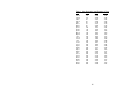
Table 1. Solar Declination and Equation of Time.
Date
Jan 1
Jan 10
Jan 20
Jan 30
Feb 9
Feb 19
Mar 1
Mar 11
Mar 21
Mar 31
Apr 10
Apr 20
Apr 30
May 10
May 20
May 30
Jun 9
Jun 19
Jun 29
Jul 9
Jul 19
Jul 29
Aug 8
Aug 18
Aug 28
Sep 7
Sep 17
Sep 27
Oct 7
Oct 17
Oct 27
Nov 6
Nov 16
Nov 26
Dec 6
Dec 16
Dec 26
DOY
1
10
20
30
40
50
60
70
80
90
100
110
120
130
140
150
160
170
180
190
200
210
220
230
240
250
260
270
280
290
300
310
320
330
340
350
360
D-rad
-0.403
-0.386
-0.355
-0.312
-0.261
-0.202
-0.138
-0.071
-0.002
0.067
0.133
0.196
0.253
0.304
0.346
0.378
0.399
0.409
0.406
0.392
0.366
0.331
0.286
0.233
0.174
0.111
0.045
-0.023
-0.091
-0.157
-0.219
-0.275
-0.324
-0.363
-0.391
-0.406
-0.408
15
ET-hour
-0.057
-0.123
-0.182
-0.222
-0.238
-0.232
-0.208
-0.170
-0.122
-0.072
-0.024
0.017
0.046
0.060
0.059
0.043
0.015
-0.019
-0.055
-0.085
-0.103
-0.107
-0.094
-0.065
-0.022
0.031
0.089
0.147
0.201
0.243
0.268
0.273
0.255
0.213
0.151
0.075
-0.007
4. Keyboard Operation
This section is designed to familiarize the user with the
Ceptometer's function keys. More in depth discussion
of the methods described briefly here can be found
later in this chapter.
Overview of Functions
Function 1:
Function 2:
Function 3:
Function 4:
Function 5:
Function 6:
Function 7:
Function 8:
PAR Measurement; A is the sample
button and B averages the readings
and sends them to memory.
Sunfleck Measurement; A is the
sample button and B averages the
readings and sends them to
memory.
Views previously stored PAR
readings and reads PAR and
sunflecks unattended.
Views previously stored sunfleck
readings and reads sunflecks and
PAR unattended.
Continuously samples PAR and
sunflecks and displays readings.
Sets the Sunfleck to the correct
time. The A key controls the hours
and the B key controls the minutes.
Sets single element mode for point
sensor use and sets the sunfleck
threshold.
Downloads and erases memory.
16
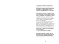
The Ceptometer is controlled by the three keys on the
cover, located just below the display. The key on the
left is the function key and is used to switch functions.
Keys A and B, located in the middle and right of the
cover respectively, affect the Ceptometer's mode of
operation within a function. All of the Ceptometer's
modes are mapped out on the keyboard.
When the batteries are installed, the Ceptometer's
microprocessor is always on to update the clock,
check the keyboard, and maintain the memory, but
the display closes after 7 minutes without keyboard
operation. Any button may be pressed to activate the
display.
8
7
6
5
4
3
2
1
FUNCTION
A
B
1 PAR
2 Sunfleck
3 Auto PAR
4 Auto Sunfleck
5 Continuous
6 Time set
7 Threshold or
Single Sensor
8 Erase or Send
sample
sample
read
read
hold
hours
set
average
average
read
read
store
minutes
erase
set
send
SUNFLECK
CEPTOMETER
Decagon
Pullman, WA
Made in USA
Figure 3. Cover of the Sunfleck Ceptometer.
17
Any of the eight functions of the Ceptometer may be
selected by pressing the function key. A small arrow
above the display corresponding indicates the
selected function.
Note: Regardless of the mode, both Sunfleck and
PAR readings are stored in final memory. The
functions only alter the displayed readings.
8
7
6
5
4
3
2
Figure 4. Function Indicator Arrow.
18
1
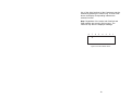
Function 1: PAR Measurement
Press the function key until the display arrow is
pointing to number one. In this mode, the A key is the
sample key. Each time this key is pressed, the
Ceptometer will take a new PAR reading. The
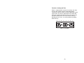
previous readings will be saved in a short-term
memory until an average is taken. The sample
number is shown on the left side of the display and
the PAR measurement is shown on the right.
8
7
6
5
4
3
2
1
Figure 5. Sample Number and PAR Measurement.
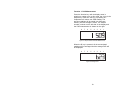
When the B key is pressed, all the accumulated
readings will be averaged and the average PAR will
be displayed.
8
7
6
5
4
3
Figure 6. Average PAR.
19
2
1
Pressing the B key a second time will store the
average reading in memory. Pressing the A key clears
all readings and resets the sample counter. If the A
key is pressed before the average reading is stored in
memory, the average will be erased.
8
7
6
5
4
3
2
1
Figure 7. Memory Indicator: Indicates 11 readings stored
in memory.
Function 2: Sunfleck Measurement
Function two is similar to function one, but the number
appearing on the right side of the display is the
sunfleck fraction. Sunfleck fraction is given as a
percentage of the sensors exposed to a radiation
level greater than the set threshold. For a more
detailed discussion of sunfleck fraction, please refer to
page 43 of this manual. The A key is the sample key.
The B key averages the readings and sends the
averaged reading to memory. Before making sunfleck
fraction measurements, a threshold will need to be
set. Refer to function seven.
20
Function 3:
Unattended PAR Measurement
and Display of PAR Memory.
This function displays previously stored PAR readings
and measures PAR unattended. Stored readings can
be read by pressing either the A or B keys. The A key
displays progressively earlier readings while the B key
displays progressively later readings. The readings are
shown on the right of the display and the time of
sampling is displayed on the left.
To begin the unattended reading mode, press the A
and B keys simultaneously. The Ceptometer will
display the auto mode indicator. (Refer to Figure 9).
Every minute, the instrument will automatically sample
PAR and sunflecks, but the display will only show
PAR. Function 4 is identical to function 3 and will only
show sunflecks. Each half hour, the thirty samples will
be averaged and stored in memory. The Ceptometer
will remain in automatic mode until either the A or B
key is pressed.
8
7
6
5
4
3
2
1
Figure 8. Time and Stored Reading.
8
7
6
5
4
3
2
Figure 9. Unattended PAR Indicator.
21
1
Function 4:
Unattended Sunfleck
Measurement and Display of
Sunfleck Memory
Function four displays previously stored sunfleck
readings and measures sunflecks unattended. This
function is similar to function three and the keys are
used in the same way. As in function two, a threshold
should be set before sunfleck measurements are
taken. Refer to function seven.
Function 5:
Continuous Sunfleck and PAR
Readings
Function five continuously samples both PAR and
Sunfleck and displays the readings. The PAR
measurement is shown on the right of the display and
the sunfleck measurement is shown on the left. As
measurement conditions change, so will the readings,
but they may be held by pressing the A key. Pressing
the A key again will release the values. Held values
can be sent to memory by pressing the B key and
stored values can then be viewed by using functions
three and four.
8
7
6
5
4
3
2
1
Figure 10. Continuous Sunfleck and PAR measurements.
22
Function 6: Setting the Time
When a measurement is stored in memory, the time
in hours and minutes will be stored along with it.
Function six can be used to set the Ceptometer to the
correct time. The A key controls the hour value and
the B key controls the minutes. The clock can be set
by either moving one hour or minute at a time by
pressing the key once, or moving rapidly by holding
down the key.
8
7
6
5
4
3
Figure 11. Time Setting.
23
2
1
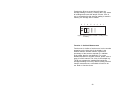
Function 7: Setting the Threshold
Function seven is used to set the threshold and
determine whether one or all of the sensors will be
sampled. For applications of the threshold and line
vs. single sensor operation, refer to chapter six
beginning on page 31 of this manual.
Threshold refers to the lowest PAR value in µmoles
that will be sampled. Any number below the chosen
value will not be counted in the measurement.
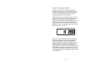
Pressing the A key sets the threshold manually; it will
be set equal to half of the highest reading of any
sensor on the probe. The letter "H" is shown on the
display to indicate a threshold function along with the
threshold setting in µmol m-2 s-1 .
8
7
6
5
4
3
2
1
Figure 12. Threshold Indicator and Setting.
The B key is used for both automatic threshold and
single sensor setting. In the automatic threshold
mode, the Ceptometer will find the highest light
reading on the probe and set the threshold at half of
that value.If there is a difference in light along the
probe, the sunfleck reading will be displayed as a
percentage less than 100 if the lower value falls below
the threshold. If the light on the probe is even, the
reading will be 100 percent, regardless of the strength
of the light and assuming the reading is greater than
the set threshold.
24
In the single sensor mode, only one sensor at the tip
of the probe will respond to light. This allows the
instrument to be used as a point sensor. In this mode,
the readings in functions one through five will be
single sensor readings. The sunfleck reading will be
either "1" or "0," indicating that the reading is above
or below the manually set threshold.
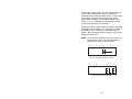
Pressing the B key shifts between automatic threshold
and single sensor settings. The automatic threshold is
indicated by an "H" followed by two dashes on the
display. When the single sensor setting is chosen, the
display will read "ELE."
NOTE: The automatic threshold cannot be used in the
single sensor mode. The threshold must be
manually set before using this option.
8
7
6
5
4
3
2
1
Figure 13. Automatic Threshold Indicator.
8
7
6
5
4
3
2
Figure 14. Single Sensor Indicator.
25
1
Function 8:
Send/Erase Memory and
Individual Sensor Dump
Function eight is used to send stored readings to an
external device or to erase the memory. Pressing the
B key sends the data via an RS-232 interface cable to
the external device. The sample numbers on the
display will continually update until the transaction is
complete. This transaction can be interrupted at any
time by pressing the A key. To erase the memory,
hold down the A key and press the B key.
If the memory is empty, individual sensor PAR
readings may be sent to an external device. This
option will not work if any data is stored in the
memory. To send these readings, select function five.
Choose desired values by pressing the A key to hold
them. Return to function eight. This move must be
direct; if function eight is passed, the reading will
be lost and must be made again. Prepare the
computer or other external device to receive the data.
Press the B key to send the individual sensor readings
to the prepared file. Refer to chapter nine for more
information about interfacing with a computer.
8
7
6
5
4
3
2
1
Figure 15: Sending Memory to an External Device.
26
5. Measurement Tips
❑ When measuring with the Ceptometer, the
instrument should be kept fairly level. This is less
critical below the canopy; however, it should be
followed as closely as possible as some of the
radiation below the canopy may be direct beam.
❑
Since light below a canopy is extremely variable,
several samples are necessary for reliable
averages.
❑
When using sunfleck inversion methods, the
instrument should be left in the same position. If
the instrument is moved, errors may result in data
collection.
❑
In canopies with clumped or row structures, it is
important to take samples that show no favoring
of within-row or between-row areas. In these
cases, it is best to sample with the probe of the
Ceptometer placed perpendicular to the row. If
row spacing is different from the probe length, the
probe can be placed diagonally to get a
representative sample.
❑
In tall canopies and canopies having small leaves,
overlapping penumbra make measurements of
sunfleck fraction unreliable. Inversion to obtain
leaf area index must therefore be performed using
measurements of transmitted PAR.
27
Discussion of the Effects of Non-Random
Distribution of Canopy Elements on LAI
Measurements in situ
There has been much discussion concerning inversion
methods to obtain leaf area index. Since all inversion
methods rely on the assumption that elements of a
canopy are randomly dispersed in space, errors in the
measurement of leaf area index may result from a
non-random arrangement of canopy elements. This is
especially true for canopies with heliotropic leaves,
conifer forests, row crops before canopy closure or for
canopies which never close, as in desert vegetation.
The degree of error in measurement is a result of the
canopy's deviation from this random dispersion
assumption.
In past studies, LAI has been used to relate both
actual biomass area and the interception of PAR by a
plant canopy. Chen et. al. (1991) have proposed
another view regarding LAI in which L, the actual
biomass area, was related to a new term, Le , which
represents the actual orientation of the canopy
elements relating to the interception of PAR at a given
angle. In situ measurements of LAI using
hemispherical photography were equated with this
new term, "effective plant area index" (Le ), which was
defined as
Le = ΩL
where L represents the actual leaf area index (equal
to a harvested leaf area measurement) and Ω refers
to a clumping index resluting from the non-random
distribution of canopy elements.
28
When a canopy displays random dispersion, Ω is
unity; however, when a canopy is clumped, Ω is not
unity. In this equation, Le refers to the actual canopy
element orientation. For example, in a randomly
dispersed canopy, L would be equal to Le (figure 1), in
an underdispersed canopy (clumping), L would be
greater than Le (figure 2), and conversely, in an
overdispersed canopy, L would be less than Le (figure
3). Refer to page 30 for illustrations.
The purpose of this discussion is to expose the user
to possible errors that may occur when making LAI
measurements in situ. When setting up an
experiment, the user should carefully examine the
desired end result. If one is interested in the
interception of PAR within a canopy, the result of the
inversions given in this manual will be correct in
reaching Le . The leaf or plant area index that is
calculated through inversion will be an accurate
portrayal of the canopy's structure and orientation with
respect to light interception. In this instance, while
clumping effects within the canopy remain present,
these effects do not cause error with regard to light
interception and the effective area index for that
situation. Alternately, if the user is interested in
obtaining the actual biomass represented by L in this
discussion, all measurements should be performed so
that the effects of clumping are minimized. This can
be accomplished by modeling the clumping factors of
the canopy or by measuring only at certain times of
day or at positions within the canopy that directly
minimize the clumping effects.
29
Figure 1: Randomly Dispersed
L=Le
Figure 2: Underdispersed
L>Le
Figure 3: Overdispersed
L<Le
30
6. Applications
The Sunfleck Ceptometer is useful for a number of
applications including the measurement of average
and intercepted PAR and the recording of sunfleck
occurrences. From these measurements, canopy
structure can be estimated.
PAR
PAR (photosynthetically active radiation) is generally
considered to be the radiation in the 400 to 700
nanometer waveband. It represents the portion of the
spectrum that plants can use for photosynthesis. In
the PAR waveband, irradiances can vary from full sun
to almost zero over the space of a few centimeters
and reliable measurement of PAR requires many
samples at many locations under the canopy.
Measuring Average and Intercepted PAR
Monteith (1977) observed that dry matter production
of a plant canopy is directly related to the amount of
photosynthetically useful radiation intercepted by the
canopy. Dry matter production is modeled as the
product of three terms:
P = efS
where P is the amount of dry matter produced, S is
the flux density of incident radiation intercepted by the
crop, and e is a conversion efficiency. Conversion
efficiency and fractional interception are determined
by crop physiology and management.
31
Incident solar radiation is the only environmental
factor. If f and S are monitored over the period of
growth of a crop, and P is measured at harvest, e can
be determined.
The results of experimental treatments or the
influence of genetics can be interpreted in terms of
their effect on
e and f.
The radiation incident on a canopy can be absorbed
by the canopy, transmitted through the canopy and
absorbed or reflected at the soil surface, or reflected
by the canopy. In principle, only PAR absorbed by the
canopy is useful in producing dry matter, so f should
be the fractional absorption. If t is the fraction of
incident radiation transmitted by the canopy, r is the
fraction of incident radiation reflected to a sensor
above the canopy, and r s is the reflectance of the soil
surface, then the absorbed radiation fraction is
calculated from:
f = 1 - t - r + trs
(1)
The last two terms are often ignored and fractional
interception is approximated by:
f=1-t
(2)
The error resulting from this approximation is usually
small when t, r, and rs are measured in the PAR
waveband, because most of the PAR is absorbed.
The error becomes much more significant when
measurements of total solar radiation are used
because of large scattering coefficients of leaves for
near infrared radiation.
32
As a first-order estimate of error, assume that
r=(1-t)rc+trs
(3)
where rc is the reflectance of the vegetation. The first
equation becomes:
f = (1 - t)(1 - rc)
(4)
The error resulting from using the second equation is
approximately equal to rc, which is typically less than
0.05 in the PAR waveband. Since the Ceptometer's
sensors are sensitive only to radiation in the PAR
waveband, equation 2 will generally be accurate for
making measurements of intercepted radiation.
However, measurement of the other terms needed for
equation 1 is simple and will also be explained.
Sampling for Fractional Interception
Select function one. For specific instructions
concerning function one, refer to page 18 of this
manual. The measurements needed for fractional
interception are those from which t, r, and rs are
calculated. If S is the PAR reading from an upwardfacing Ceptometer above the plant canopy, R is the
reflected PAR above the canopy (inverted Ceptometer
above the crop), T is the upward-facing Ceptometer
below the plant canopy, and U is the reflected PAR
from the soil surface, then t, r, and rs can be
calculated from:
t = T/S
(5)
r = R/S
(6)
rs = U/T
(7)
33
Assume only t needs to be known. Measure S above
the crop canopy. Level the Ceptometer above the
canopy using the bubble level and then press the A
key. The reading appearing on the right of the display
is S. This value can be stored in memory by pressing
the B key twice. Press the A key again to clear the
display.
Measure T by placing the Ceptometer below the plant
canopy, being careful to place it below all of the
leaves. Try to keep the instrument level. Since the
light below the canopy is extremely variable, several
samples at different locations will be necessary for a
reliable reading. The number of necessary samples
can be determined by taking, for example, 10
readings and computing the coefficient of variation
from:
CV = [Σ(xi - x)2 / (n - 1)]1/2 / S
(8)
where n is the number of samples taken. The error in
any measurement of t will be CV divided by the
square root of the number of samples. Usually, a
number around 10 should suffice. Press the A key to
take a reading. Each of the readings will appear on
the left of the display.
In canopies with a clumped or row structure, it is
important that samples show no favor of between-row
or within-row areas. It is best to sample with the probe
perpendicular to the row. If the row spacing is different
from the probe length, the probe can be placed
diagonally to get a representative sample. The
readings taken can be averaged by pressing the B
key. This reading is the T value. Pressing the B key a
second time stores the reading in memory. The
fractional transmission for the canopy, t, can now be
calculated from equation 5.
34
This calculation would normally be generated by a
computer program after the data from all of the
samples have been sent to the computer. However, it
is important to set up some kind of sampling scheme
beforehand or keep detailed notes of sampled areas
of the field plot or treatment so that they can be
compared to the readings stored in the instrument's
memory.
To find r, invert the Ceptometer at a height of 1-2
meters above the crop canopy. Leveling is not critical
for this measurement, since the radiation reaching the
sensor is not directional. Clear the display by pressing
the A key. Press the A key a second time to take a
reading. The display shows the R value. Multiple
readings are not necessary since R is not usually
variable. Press the B key twice to store the reading in
memory. Calculate r from equation 6 using the
previously recorded S value.
To find rs, invert the Ceptometer over the soil below
the canopy and take measurements at several
locations. Average and store these measurements as
before. This reading is the value U. Calculate rs from
equation 7 using U and T. A value in the range of 0.1
to 0.2 should be obtained, but it is possible that the
light level below the canopy will be so low that U will
not be accurately measured. If a value outside of the
expected range is obtained, there will be negligible
error in f by assuming
r = 0.15. As mentioned before, evaluation of
intercepted radiation normally involves the
measurement of t.
Only measurements below the canopy have been
discussed. Obviously, measurements throughout the
canopy are possible. Profiles of interception with
height can be useful in determining at what location
most of the photosynthesis is occurring in the canopy.
35
Unattended Recording of Transmitted PAR
The value of f in equation 1 can vary with sun
elevation, since t depends on elevation angle.
Fractional interception should be an integrated value
averaged over the growing season. While the reading
obtained at a particular time is closely related to this
average value, readings need to be taken over a full
day to find the true integrated value of t. Two
measurements are needed;
T at various times of the day, and S integrated over
these same times.
We recommend that the data for S be obtained by
recording the output of another Ceptometer or a
SunLink PAR Probe. Both instruments have identical
spectral and cosine responses. A PAR point sensor
may also be used, or the data may be obtained by
calculating PAR from incident solar radiation. To do
so, multiply the total short- wave flux density (W m-2 )
by 2.1 to convert to µmol m-2 s-1 . This calculation can
be verified by comparing these estimates to spot
measurements with the Ceptometer placed above the
plant canopy.
To obtain data for T, support the Ceptometer in the
canopy, select function three, and press the A and B
keys simultaneously. Readings will be taken
automatically every minute, and then averaged and
stored in memory every 30 minutes. Press either the
A key or the B key to stop logging. Readings can be
reviewed by pressing the A and B keys to move back
and forth through the memory.
36
Survey Sampling of Average Line PAR
Select function five. The value appearing to the right
of the display is the average PAR over the length of
the probe. The value will be updated continuously
until the A key is pressed to hold the present reading.
This reading may be stored in memory by pressing
the B key, or the user may return to the continuous
readings by pressing the A key again.
Using PAR to Determine Leaf Area Index
Ceptometer users may want to use sunfleck
measurements to determine plant canopy parameters
such as leaf area index and leaf angle distribution.
The theory for obtaining LAI and leaf angle
distribution from these measurements is widely
published. However, the theory is incomplete in some
respects and this affects the accuracy of canopy
parameters predicted from sunfleck measurements.
Errors are greatest when LAI is high and/or when the
canopy is tall. The sunfleck inversion fails completely
when the sky is overcast and there are no sunflecks.
Our research has shown that an inversion using
transmitted PAR is much more reliable under almost
all conditions than an inversion using sunfleck fraction.
We recommend that this PAR inversion be used
instead of the inversion based on sunfleck fraction.
The PAR measured by the Ceptometer within a plant
canopy is a combination of radiation transmitted
through the canopy and radiation scattered by leaves
within the canopy. A complete model of transmission
and scattering is given by Norman and Jarvis (1975),
but it is very complex and not suitable for inversion.
37
The Norman-Jarvis model was used to test and fit two
simpler models which are more easily inverted.
Equation 1 is a simple light scattering model
suggested by Goudriaan (1988). It gives the fraction
of transmitted PAR, t (ratio of PAR measured below
the canopy to PAR above the canopy), below a
canopy of LAI, L, as
(
)
(
τ = f b exp − aKL + (1 − f b ) exp −0.87 aL
)
(1)
Here fb is the fraction of incident PAR which is beam,
a is the leaf absorptivity in the PAR band (typically
around 0.9), and K is the extinction coefficient for the
canopy. The extinction coefficient can be modeled in
various ways. Assuming an ellipsoidal angle
distribution function (Campbell, 1986), then
K=
(x
2
+ tan 2 θ
)
1/ 2
x + 1. 744 ( x + 1. 182 )
−0.733
(2)
where θ is the zenith angle of the sun and x is a leaf
angle distribution parameter. When x=1, the angle
distribution is spherical, and K simplifies to
K=
1
2 cos θ
John Norman suggested a different equation for
predicting scattered and transmitted PAR.


 A(1 − 0.47 f b ) L 
τ = exp 

 1 − 1  f b − 1 
 

2K 
where A = 0.283 + 0.785a - 0.159a 2 .
38
(3)
Both equations predict canopy PAR within a few
percent of values from the complete Norman-Jarvis
model. Equation 1 is slightly more accurate, but
equation 3 is much easier to invert to obtain L. The
difference in accuracy of the two equations is smaller
than other incertainties in the method, so equation 3
will be used to determine LAI. Inverting equation 3
gives:
1 


1 − 2 K  f b − 1 ln τ
L=
A(1 − 0.47 f b )
39
(4)
Applications and Examples
PAR was measured above a barley canopy of
391µmol m-2 s-1 on an overcast day. The average of
several measurements below the canopy was 62
µmol m-2-1. The transmission, τ, is therefore 62/391 =
0.159. Since the day was overcast, fb = 0. If a = 0.9,
then A = 0.86. From equation 4, L = - ln (0.159)/0.86
= 2.14. Because the measurement was made under
overcast skies, it was not necessary to have canopy
structure information or solar elevation angle.
Measurements on overcast days are the simplest for
LAI determination and do not require assumptions
about canopy structure.
The next example uses measurements on a sunny
day. 1614 µmol m-2 s-1 was measured above a pea
canopy and 80 µmol m-2 s-1 under the canopy. The
fraction of PAR transmitted by the canopy was
therefore
τ = 80/1614 = 0.05. The solar zenith angle was 30o .
The fraction of diffuse radiation was measured by
switching the Ceptometer to single sensor mode and
taking a reading with the leveled probe in full sun and
another reading with the sensor at the tip of the probe
shaded by a 10 centimeter diameter shade at a
distance of about 1 meter. The ratio of the shaded to
unshaded readings was 0.119, which is the diffuse
PAR fraction. The beam fraction was fb = 1 - fd =
0.881. The A value for equation 4 is again 0.86. "x"
for the canopy is unknown, but unless leaves have
obvious horizontal or vertical tendencies, a spherical
distribution can be assumed and x be set equal to 1.
For a zenith angle of 30 degrees, this gives K =
0.577. Substituting these values into equation 4
results in L = 5.2.
40
Final Comments
While leaf area estimates can be made under either
clear or overcast skies, the clear sky estimate requires
that you guess a value for x. The overcast sky
measurement may therefore be more reliable. Spatial
variability is a big problem in canopies, and
measurements at several locations should always be
used to determine LAI.
Spectral and Cosine Response
The Ceptometer is limited in ideal PAR response
because of its deficiencies in the blue spectrum.
These deficiencies are insignificant when working with
normal plant canopy environments and solar
radiation. However, the Ceptometer should not be
used as an absolute PAR sensor when the
environment being studied has a significant blue
emphasis in its radiation composition. Examples of
this blue component would include the measurement
of blue skies while the sensors are shaded from direct
beam radiation or artificial lighting that contains a
strong blue component like metal halide.
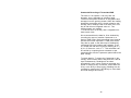
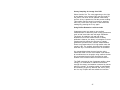
The two graphs on the following pages show the
responses of the Ceptometer sensors. Spectral
response of the photodiodes lies almost entirely within
the PAR waveband. The response approximates an
ideal quantum response, but drops to zero at about
680 nm rather than 700 nm, and is somewhat low in
the blue region. If the radiation is entirely blue skylight,
the GaAsP photodiode reads about 20% lower than
the PAR sensor, but under normal sun and light,
cloudy skies, or in crop canopies, errors due to limited
spectral response are negligible.
41
42
Relative Response
0
0.2
0.4
0.6
0.8
1.0
400
500
Wavelength (nm)
GaAsP Photodiode
Quantum
600
700
43
Response Ratio
0.70
0.75
0.80
0.85
0.90
0.95
1.00
0
10
20
40
50
Horizontal
60
Zenith Angle (degrees)
30
Vertical
70
80
90
7. Sunflecks
Sunflecks refer to the bright areas under the canopy
where direct beam solar radiation penetrates without
dissipation by the canopy. The size, shape, duration,
and peak photon flux of a sunfleck depends on the
height and precise arrangement of vegetation within
the canopy as well as the position of the sun in the
sky. Fraction measurements of a ground covered by
sunflecks can be used with inverse methods to
determine important characteristics of canopy
structure.
The sun approximates a point source of radiation
which can be used on clear days to probe the canopy
and obtain information on canopy cover and canopy
geometry. The information needed to determine
these canopy properties is the fraction of the area
under the canopy which is covered by sunflecks, or
the gap fraction of the canopy. For canopy cover, only
measurements at high sun angles are needed since
cover is the fraction of the ground covered by a
vertical projection of the canopy onto it. Sunfleck
measurements at several sun angles are needed to
determine other canopy characteristics.
Note: When using sunflecks for inversions, it is critical
that the instrument be placed in exactly the
same location for each reading. It is therefore
strongly recommended the unattended mode
of data collection be used.
The sunfleck measurement can also be used to
determine intercepted radiation for a canopy.
44
The sunfleck measurement is faster than the PAR
measurement since the sunfleck measurement does
not require finding the ratio of measurements below
the canopy to measurements above it. It also has
advantages on days where incoming radiation varies
over short time periods, since light levels needed for
making calculations are all measured at one time. The
method cannot be used on overcast days or in
canopies with overlapping penumbra since it relies on
distinct shadows to make the measurement.
(Penumbra are the partial shadows which surround
the shadows of objects illuminated by the sun or any
other source of finite size, and are the result of the
sun not being a point source of light).
Setting the Threshold
A proper threshold level must be established before
accurate sunfleck measurements can be made. At
each sunfleck measurement, the sensors in the probe
are scanned by the microprocessor, and the reading
of each sensor is compared to the established
threshold. The microprocessor counts the number of
sensors above the threshold, divides this value by the
total number of sensors in the probe, and then
displays the reading as a percentage. Two types of
threshold settings are possible. When a sample is
taken by the instrument in the automatic threshold
setting, the microprocessor scans the set of readings,
finds the highest one and sets the threshold at half of
this value. If the highest light value on the probe
changes as different samples are taken, the threshold
will also change. As long as the sunflecks are large
enough for at least one sensor to be in full sun the
automatic threshold setting is the simplest and most
reliable setting to use. It also measures the correct
size of sunflecks with penumbra, as long as they do
not overlap.
45
The manually set threshold must be used for dense
canopies when there is a possibility that not even one
sensor will be in full sun during a scan. Select function
seven and press the A key. The probe is scanned and
the threshold is set at half of the value of the highest
sensor reading. The threshold value is displayed in
-2 -1
µmol m s . If a different threshold level is desired,
select the location of the probe when the A key is
pressed.
The manually set threshold will remain until it is reset.
The user should experiment with the manual
threshold mode before taking serious data, as it may
take some time to learn to use this setting effectively.
Measurements of low sunfleck fraction which cause
the Ceptometer to register a high value are an
indication that this mode may need to be used. The
instrument reads 100.0 in full sun, but it also reads
100.0 in full shade, since it determines the
percentages by comparing the highest reading on the
probe. It is only when there is variation along the
probe that it can detect sunflecks.
Sampling for Sunfleck Fraction
Sampling for sunfleck fraction is similar to sampling
PAR under the canopy. Select function two. Place the
probe under the canopy and press the A key. Many
samples are needed because of the large spatial
variation in sunfleck fraction. Leveling is not important
for sunfleck measurements, and it is sometimes
desirable to tip the probe in the direction of the sun
when sun angles are low so that a larger reading is
obtained. The sunfleck fraction is shown on the right
of the display and the number of samples taken is
shown on the left. After 10 to 20 samples are taken,
press the B key to average and display the reading.
46
The number of samples needed for a given precision
can be estimated using equation 8 on page 34. To
store the reading, press the B key again. In the
sampling modes of functions one through five, both
PAR and sunfleck fraction are read, averaged, and
stored, but only one reading (PAR in function one and
three, and sunfleck fraction in function two and four) is
displayed.
Unattended Recording of Sunfleck Fraction
To record sunfleck fraction unattended, select function
four. Press the A and B keys simultaneously to begin
readings. Readings will be taken every minute
automatically and stored in memory every 30
minutes. The display will show time on the left and the
sunfleck fraction on the right. To stop data collection,
press either the A or B key. The readings can be
reviewed by pressing the A and B keys to move
backward and forward through the memory.
Survey Sampling of Sunfleck Fraction
Select function five. A continuous sunfleck fraction is
shown on the left of the display. Press the A key to
hold the reading and the B key to store the reading in
memory. This mode is often used to check a canopy's
variability or to determine which threshold mode to
use.
47
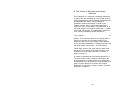
8. The Theory of Sunflecks and Canopy
Structure
If the elements of a canopy are randomly distributed
in space, then the probability of a ray of light or other
probe penetrating the canopy without interception can
be calculated from theory. The probability of
penetration without interception is equal to the
sunfleck fraction, which is the beam transmission
coefficient, τ(Θ), for the canopy. The parameter, Θ ,is
the zenith angle of the probe or solar beam. τ usually
varies with zenith angle. The transmission coefficient
for a canopy of randomly placed elements is:
τ(Θ) = exp(-KL)
(1)
where L is the leaf area index of the canopy (area of
leaves per unit area of soil surface) and K is the
extinction coefficient for the canopy, which depends
on the leaf angle distribution of canopy elements, and
the zenith angle of the probe. τ is sunflecks/100.
Zenith angle refers to the angle the sun makes with
respect to a line vertical to the earth's surface. A full
description of zenith angle and how to measure it
begins on page 11.
A number of expressions have been proposed for K.
The most useful is from Campbell (1986) where the
angle distribution of canopy elements is assumed to
be ellipsoidal. One can picture the angle distribution of
area in a plant canopy to be similar to the angle
distribution of area on the surface of oblate or prolate
spheroids, or spheres.
48
The equation for K is:
K=
(x
2
+ tan 2 Θ
)
1
2
x + 1. 744 ( x + 1. 182 )
−0.733
(2)
The parameter, x, is the ratio of the length of the
horizontal to the vertical axis of the spheroid, and can
be measured as the ratio of the projected area of an
average canopy element on a horizontal plane to its
projection on a vertical plane. Extinction coefficient is
plotted as a function of zenith angle for various values
of x. (See figure 16). At a zenith angle of about 57
degrees, the extinction coefficient is near unity for all
canopies. When leaves are horizontal (large X), the
extinction coefficient, K, is unity for all elevation
angles, but as X decreases, K becomes smaller at
large zenith angles and larger at small zenith angles.
Equation 1 can be used in various ways to determine
the leaf area index, and possibly also the leaf angle
distribution function for a canopy. The simplest
application is that of Bonhomme et al. (1974). Since
K=1 for zenith angles near 57 degrees, the inversion
of equation 1 is simple and gives:
L = -ln(τ57)
(3)
If a sunfleck measurement is made when the zenith
angle is about 57 degrees, equation 3 can be used
directly to find L.
If measurements of the transmission coefficient, τ, are
made at several elevation angles, a simple method
from Lang (1987) can be used.
49
The measurements of τ are used to compute y = cos
Θ ln τΘ. These are regressed on Θ (in radians), giving
a slope, B, and an intercept, A. The leaf area index is
given by:
L = 2(A+B)
(4)
An approximate value for x is x = exp(-B/0.4L).
Example: Sunfleck readings were obtained as follows:
Θ-degree
35
41
55
Θ-radian
0.61
0.72
.096
τ
0.21
0.18
0.10
-cosΘ ln τ
1.28
1.29
1.32
Linear Regression gives:
A = 1.21
B = 0.12
L = 2(1.21 + 0.12) = 2.64
x = exp(-0.12 / 0.4 x 2.64) = 0.9
Note: Θ can be measured by placing a stick of length,
y, vertically in the ground and measuring the
shadow length, x, on a horizontal surface.
tan Q = x/y so Θ = tan -1(x/y).
50
A more precise method for finding x is as follows. We
would like to find values for x and L which minimize:
F = Σ(ln τi + Ki L)2
subject to the constraint, x>0, where τi are
transmission coefficients measured at several zenith
angles, and τi Ki are the extinction coefficients for the
corresponding angles. A BASIC computer program
which finds L and x from measured sunfleck fraction
data is outlined on the following page.
51
A Computer Program to Find LAI and LAD
from Sunfleck Fraction Measurements
10 REM ******* ELLIPSOIDAL EXTINCTION COEFFICIENT
20 DEF FNK(Z,X)=SQR(X*X+Z*Z)/(x + 1.774*(x + 1.182)^(-0.733))
35 REM ******* Z IS TAN(ZENITH ANGLE)
30 REM *******
40 PI=3.14159:DX=0.1
50 INPUT "NUMBER OF ZENITH ANGLES";NZ
60 DIM Z(NZ),T(NZ)
70 FOR I=1 TO NZ
80
PRINT "ZENITH ANGLE";I;" - DEGREES";:INPUT Z(I)
90
PRINT "TRANSMISSION AT ";Z(I);"DEG";: INPUT T(I)
100 Z(I)=TAN(Z(I)*PI/180):T(I)=LOG(T(I))
110 NEXT
120 REM ******* FIND X USING BISECTION METHOD
130 XMAX=10:XMIN=.1:X=1
140 S1=0:S2=0:S3=0:S4=0
150 FOR J=1 TO NZ:TZ=Z(J)
160
KB=FNK(TZ,X):DK=(FNK(TZ,X+DX)-KB)
170
S1=S1+KB*T(J):S2=S2+KB*KB:S3=S3+KB*DK:S4=S4+DK*T(J)
180 NEXT
190 F=S2*S4-S1*S3 :PRINT X,F
200 IF F<0 THEN XMIN=X ELSE XMAX=X
210 X=(XMAX+XMIN)/2
220 IF (XMAX-XMIN)>.01 THEN GOTO 140
230 REM ******* FIND LAI AND PRINT RESULTS
240 L=-S1/S2:PRINT "LEAF AREA INDEX=";L
250 PRINT "RATIO OF VERTICAL TO HORIZONTAL
PROJECTIONS=";X
260 PRINT
270 PRINT "ZENITH ANG.","MEASURED T","PREDICTED T"
280 FOR J=1 TO NZ
290
PRINT ATN(Z(J))*180/PI,EXP(T(J)),EXP(-FNK(Z(J),X)*L)
300 NEXT
52
Correction of Sunfleck and Intercepted Radiation
for Sun Angle
Sunfleck fraction, τ, measured at one zenith angle,
can be used to predict sunfleck fraction or radiation
interception for other zenith angles. For example, a
measurement might be made at Θ = 32o from which
cover (1 - transmission at Θ = 0) is to be calculated.
From equation 1,
ln τ1 /ln τ2 = K1 /K2 = p
(5)
so
τ(Θ1 ) = τ(Θ2 )p
(6)
Calculate p from equation 2
p = [(x2 + tan2 Θ1 )/(x2 + tan2 Θ2 )]1/2
(7)
If Θ1 = 0, p = [x2 /(x2 + tan2 Θ2 )]1/2 .
If x is not known, assume x = 1.
Example: From the previous measurements, find the
canopy cover. Take Θ = 35o , τ = 0.21, and x = 0.9.
p = [(0.92 )/(0.92 + tan2 35)] = 0.79
τ(0) = 0.210.79 = 0.29
Cover = 1 - τ(0) = 1 - 0.29 = 0.71.
53
Intercepted radiation averaged over an entire day can
be estimated from:
f = 1 = τd
(8)
where τd is the transmission coefficient averaged over
all elevation angles. τd can be calculated from:
(9)
-ln τd = uLv
where u and v are functions of x which can be
calculated from:
u = 1 - 0.33 exp(-0.57x)
(10)
v = 1 - 0.3 exp(0.97x)
(11)
The following table shows typical values of u and v.
v
_________
0.1
0.5
1.0
2.0
4.0
8.0
u
_________
0.699
0.745
0.816
0.903
0.963
0.989
v
_________
0.728
0.818
0.892
0.951
0.982
0.995
Table 2. Values for u and v for equation 9.
54
Combining equations 1 and 9 gives:
τd = τ(Θ)q
where q = uLv-1 /K.
Example: Calculate a value for fractional daily
interception for the crop in the previous examples.
u = 1− 0 . 33 exp ( −0. 57 × 0. 9 ) = 0. 80
v = 1− 0. 3 exp ( −0. 97 × 0. 9 ) = 0. 87
K=
(0.9
2
− tan 2 35)
1/ 2
0.9 + 1.774(0.9 + 1.182)
0.80 × 2.64 −0.13
τ=
= 1.2
0.59
τ d = 0. 211.2 = 0. 15
f = 1− τ d = 1− 0. 12 = 0. 85
55
−0.733
=
1.14
= 0.59
1.94
9. Interfacing with a Computer
Data collected and stored in the Ceptometer's
memory can be downloaded to a disk file using the
SunView software included with your instrument or the
BASIC program outlined in this chapter.
The Ceptometer's communication protocol is:
❑
Baud Rate: 1200
❑
Parity: even
❑
Data Bits: 7
❑
Stop Bits: 1
Ceptometer data is output as comma separated
values. The output signal is as follows:
5V
0V
Start
D0
LSB
D1
…
56
D7
Parity
Stop
Connections for the 9 pin connector are:
1.
2.
3.
4.
5.
5V
Ground
NC
NC
NC
6.
7.
8.
9.
5V
NC
NC
Data Out
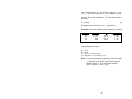
BASIC Program
5
10
20
40
45
50
60
70
80
85
INPUT "NAME OF DATE FILE";DF$
OPEN"COM1:1200,,,,CS,DS,CD" AS 1
OPEN DF$ FOR OUTPUT AS 2
T$ = INPUT$(1,#1)
ON ERROR GOTO 85
IF T$ = CHR$(127) THEN T$ = CHR$(63)
PRINT T$;
PRINT #2,T$;
GOTO 40
RESUME
57
Notes on the BASIC Program
Line 1: Prompts the program to go to line 85 if an
error occurs during the execution of the program.
Line 5: Displays "NAME OF DATA FILE?", and
assigns it to the variable DF$.
Line 10: Opens communication device 1as file
number 1. The baud rate is 1200, parity is set to the
default value, the number of data bits is set to the
default value, the stop bit is set to the default value,
the request to send is suppressed, and CS(clear to
send), DS(data set ready), and CD(carrier detect) are
set so as not to allow them to time out.
Line 20: Opens DF$ and creates a file number 2 to
receive data.
Line 40: Inputs one character at a time from the file
numbered 1 to the file or variable t.
Line 50: Checks the contents of t. If it is equal to 127,
it is changed to 63.
Line 60: Prints the contents of t to the screen.
Line 70: Prints the contents of t to the file numbered
2.
Line 80: Prompts the program to go to line 40.
Line 85: Prompts the program to resume running on
the line where an error was detected.
58
Executing the BASIC Program
Write and save the BASIC program to disk, then
execute it in the following way to avoid any
communication/buffer overflow problems:
If the program were called Sunread, type
"gwbasic sunread \C:15000" at the prompt.
This allocates 15,000 bytes to the RS-232 receiver
buffers and allows enough room for a full interface
with the Ceptometer's memory.
Note: When running the program and saving data to
disk, check to see that there is at least 40K left
on the disk. A full interface of 1200 data points
requires 22K of disk space.
59
Sunfleck SunView Software
Backing Up and Running SunView from Floppy Disk
Before using the SunView program from a floppy disk,
make a backup copy.
❑
Insert a blank formatted disk into drive A.
❑
Place the SunView disk in drive B.
❑ Type COPY B: SUNVIEW.EXE A:
To run SunView from a floppy disk:
❑
Place the floppy disk in drive A.
❑
Type A:SUNVIEW.
Note: Put the original SunView disk in a safe
place. Always run the program from a
backup copy.
60
Installing SunView to the Hard Drive
❑
Place the SunView disk in drive A.
❑
Move to your hard drive and make a SunView
directory by typing MD SUNVIEW.
❑
Move to the SunView directory (CD\SunView)
and type COPY A:SUNVIEW.EXE.
❑
Put the original SunView disk in a safe place.
❑
To run the SunView program, type
CD\SUNVIEW then SUNVIEW.
Connecting the RS-232 Cable
An optically isolated RS-232 cable is included with
each Ceptometer. This cable is specifically designed
for use with the instrument and should be used
whenever the operator wishes to download data to a
computer. Other cables will not provide correct data
output.
One end of the RS-232 cable houses a 9 pin
connector. Secure this connector to the 9 pin
receptacle on the Ceptometer. The other end of the
cable houses a 25 pin connector which needs to be
connected to the serial port of the computer at COM1.
If you are unsure which port is COM1, see your
computer operator's manual.
Note: You may use a 25-to-9 pin adapter to interface
with your computer if needed; however, the 9 pin end
of the RS-232 cable must be connected to the
Ceptometer for correct operation.
61
Downloading Memory to a Computer
Prepare your computer to receive data with the
SunView software or the BASIC program described
earlier. Press the function key until the display pointer
is stationed at function 8, then press the B key to
send the data to the computer. The sample numbers
on the display will continually update until the
transaction is complete. This transaction can be
interrupted at any time by pressing the A key.
Running SunView Software
The SunView program displays data under four
headings: Index, Time, PAR, and Sunfleck %. The
Index column refers to the data set number as it was
stored in the Ceptometer's memory.
After the required data has been sent, press F2 to
save. Press F1 to exit. If printing is a necessary
application, data sets will need to be copied to a userprovided spreadsheet. Some instructions for importing
to these spreadsheets are listed below.
Microsoft Excel: To export data to Excel, include a
.CSV extension when naming a file. You can load the
file into Excel by selecting File-Open.
Lotus 123: To export data to Lotus 123, include a
.PRN extension when naming a file. You can load the
file into Lotus 123 by selecting File-Import-Numbers.
Borland's Quattro: To export data to Quattro, include
a .PRN extension when naming a file. You can load
the file into Quattro by selecting Tools-Import. Then
select Comma & "" delimited ascii for the file format.
62
10. Maintenance
Changing the Batteries
The Ceptometer does not have a power switch. The
microprocessor is always on to maintain the memory
and update the clock, but the display closes after 7
minutes without keyboard activity.
The instrument uses 5 AA-type batteries. When the
batteries are low, an indicator will appear when the
Ceptometer is activated (the letters "LO" to the left of
the display). Press any button to clear the display. The
instrument may be used and although it will continue
its normal function, the batteries should be replaced
as soon as possible.
To replace the batteries, remove the four screws in
the cover of the Ceptometer and lift the cover
carefully. The batteries will be exposed and can be
replaced. Be sure to orient the batteries correctly. The
battery clips indicate the direction in which the
batteries should be placed.
The switch to the side of the batteries controls power
to the Ceptometer. The switch will be closed when the
cover is on the instrument and power will be on to
maintain the memory and update the clock. When the
cover is removed, the switch opens and the
instrument is reset. Data will be lost whenever the
instrument is reset. Only one sensor of the
Ceptometer has an absolute calibration; the others
are calibrated against that sensor by the
microprocessor and stored in memory. Memory is
usually lost when the batteries are replaced and the
sensors must be recalibrated.
63
Recalibrating the Sensors
The sensors should only need recalibration when the
batteries are replaced. Calibration must be performed
in bright, even sunlight on a cloudless day. Select
function seven. The display should read H - -. Hold
down the A and B keys simultaneously and press the
function key. The letters "PLL" will appear on the left
of the display, indicating that the sensors have been
recalibrated.
Note: Be sure to recalibrate the Ceptometer in the
H - - mode of function seven and not the ELE
mode. If the ELE mode is used, the instrument
will not function properly and will need to be
recalibrated.
Cleaning the Probe
The white surface of the probe should always be
clean to insure accurate readings. To clean the probe,
use a small amount of alcohol and a soft cloth. Rub
the surface until it is clean.
64
11. Return and Repair
Should anything ever go wrong with the Ceptometer,
Decagon will repair it. Just follow the instructions below
for returning the instrument.
❑ Before returning the Ceptometer, call our offices
for a Return Materials Authorization Number
(RMA#). Include this number on all
correspondence regarding the repair of your
instrument.
❑
❑
With your return, please include your RMA#, a
complete return address, the name and
department of the person responsible for the
Ceptometer, a repair budget for non-warranty
instruments, and a purchase order number.
Pack the Ceptometer carefully and mail to:
Decagon Devices, Inc.
NE 1525 Merman Drive
Pullman, WA 99163
To avoid damage during shipping, return the
instrument in the case in which it was shipped or
place adequate padding around it. NEVER
SHIP THE CEPTOMETER WITH THE
BATTERIES INSTALLED.
65
12. Questions and Answers
❑
When should I remove the batteries from my
instrument?
❍
Always remove the batteries before shipping or
traveling with the Ceptometer. If the batteries are
shifted during transit, data will be lost and cannot
be retrieved. Damage to the battery clips is also a
possibility if the batteries are shifted.
❑
Can the data I gather with the Ceptometer be
saved to an external device?
❍
Yes. Data collected and stored in the Ceptometer
memory can be downloaded to a disk file using a
BASIC program or the SunView software included
with the instrument. Please refer to page 63 of
this manual for instructions on downloading the
Ceptometer.
❑
Can I send individual PAR readings to an external
device?
❍
Yes. However, this option will not work if any data
is stored in memory. Please refer to page 26 of
this manual for instructions on this option.
66
❑
Can I use the automatic threshold setting in the
single sensor mode?
❍
No. The automatic threshold setting cannot be
used in the single sensor mode. The threshold
must be manually set before using this option.
Please refer to page 25 of this manual for more
details.
❑
"PLL" does not appear on the display after I have
calibrated. What should I do?
❍
First try your calibration technique again.
Remember to hold the keys down simultaneously
to avoid any errors. Refer to page 10 of this
manual for detailed instructions on calibration. If
this does not work, contact Decagon for technical
assistance.
❑
I accidentally recalibrated my instrument in the
ELE mode instead of the H - - mode. What should
I do?
❍
Recalibrate the Ceptometer making sure to
calibrate in the H - - mode. Refer to page 65 of
this manual for instructions on recalibraiton.
Calibrating in the ELE mode will not damage the
instrument, but will put it in the single sensor
mode, meaning that only one sensor at the probe
tip will respond to light. Future readings in this
mode will not be accurate.
❑
The display is reading "LO." What does this
mean?
❍
A "LO" reading indicates that the batteries are
running low. Press any key to clear the display.
The instrument may be used as normal; however,
the batteries should be replaced as soon as
possible.
67
❑
Pressing keys on the keypad does not activate the
display. What should I do?
❍
Reset the batteries in the battery pack. Refer to
page 64 of this manual for instructions. If this
does not solve the problem, the instrument will
need to be sent for repair. Refer to chapter 11 for
return and repair instructions.
The following is a list of problems that may indicate
other complications with the Ceptometer. If any of
these problems should occur, the instrument may
need to be returned for repair. Please contact
Decagon first for technical assistance.
❑
The instrument powers up but seems to stick
when trying to scroll through functions.
❑
The instrument powers up but the display fades a
and flickers.
❑
After calibration, the instrument reads low light
readings, but will not read above low light
readings.
68
Appendix A: Additional Information
The following is a list of references that offer more
detail concerning plant canopy characteristics.
Anderson, M.C. (1971) Radiation and crop structure.
In Plant Photosynthetic Production, Manual of
Methods (eds A. Sestak, J. Catsky and P.G. Jarvis),
Junk, The Hague, pp. 412-66.
Campbell, G.S. (1977) An Introduction to
Environmental Physics, Springer-Verlag New York
Inc., New York,
159 pp.
Campbell, G.S. (1986) Extinction coefficients for
radiation in plant canopies calculated using an
ellipsoidal inclination angle distribution. Agric. For.
Meteorol., 36, 317-21.
Campbell, G.S. and Norman, J.M. (1988) The
description and measurement of plant canopy
structure. in Plant Canopies: Their Growth, Form and
Function (ed. G. Russell), Society for Experimental
Biology, Seminar Series 29, Cambridge University
Press, New York.
Goudriaan, J. (1977) Crop Micrometeorology: A
Simulation Study, Center for Agriculture Publication
Documentation, Wageningen, The Netherlands.
Lang, A.R.G., 1986. Leaf area and average leaf
angle from transmission of direct sunlight. Aust. J.
Bot ., 34:349-355.
69
Lang, A.R.G.,1987. Simplified estimate of leaf area
index from transmittance of the sun's beam. Agric.
For. Meteorol., 41:179-186.
Lang, A.R.G. 1991. Application of some of Cauchy's
theorems to estimation of surface areas of leaves,
needles and branches of plants, and light
transmittance. Agric. For. Meteorol., 54: (in press).
Lang, A.R.G., McMurtrie, R.E., and Benson, M.L.,
1991. Validity of leaf area indices of Pinus radiata
forests estimated from transmittances of the sun's
beam.
Agric. For. Meteorol., (accepted).
Lang, A.R.G., and McMurtrie, R.E., 1991. Total leaf
areas of single trees of Eucalyptus grandis estimated
from transmittance of the sun's beam. Agric. For.
Meteorol., (accepted).
Lang, A.R.G. and Xiang Yueqin (1986) Estimation of
leaf area index from transmission of direct sunlight in
discontinuous canopies. Agric. For. Meteorol., 37,
229-43.
Lang, A.R.G., Xiang Yueqin and Norman, J.M. (1985)
Crop structure and the penetration of direct sunlight.
Agric. For. Meteorol., 35, 83-101.
Lemur, R. (1973) A method for simulating the direct
solar radiation regime in sunflower, Jerusalem
artichoke, corn and soybean canopies using actual
stand structure data. Agric. Meteorol., 12, 229-47.
70
Norman, J.M. (1979) Modeling the complete crop
canopy. in Modification of the Aerial Environment of
Crops (eds B.J. Barfield and J. Gerber), American
Society of Agricultural Engineers, St. Joseph, MI,
pp. 249-77.
Norman, J.M., and Campbell, G.S., 1989. Canopy
structure. Plant physiological ecology: Field methods
and instrumentation. R.E. Pearcy, J.R. Ehleringer,
H.A. Mooney and P.W. Rundel (eds). London,
Chapman and Hall. pp. 301-325.
Norman, J.M. and Jarvis, P.G. (1974) Photosynthesis
in Sitka Spruce (Picea sitchensis (Bong.) Carr.) III.
Measurements of canopy structure and interception of
radiation. J. Appl. Ecol., 11, 375-98.
Norman, J.M., Miller, E.E. and Tanner, C.B. (1971)
Light intensity and sunfleck-size distributions in plant
canopies. Agron. J., 75, 481-8.
Norman, J.M. and Welles, J.M. (1983) Radiative
transfer in an array of canopies. Agron. J., 63, 743-8.
Raison, R.J., Benson, M.L., Myers, B.J., Khanna, .K.,
McMurtrie, R.E., and Lang, A.R.G., 1991.Dynamics of
Pinus radiata foliage in relation to water and nitrogen
stress. II. Needle loss and temporal changes in total
foliage mass. For. Ecol. Manag., (accepted).
Ross, J. (1981) The Radiation Regime and
Architecture of Plant Stands, Junk, The Hague, 391
pp.
71
Welles, J.M., 1990. Some indirect methods of
estimating canopy structure. Instrumentation for
studying vegetation canopies for remote sensing in
optical and thermal infrared regions. (Eds N.S. Goel,
and J.M. Norman). Remote Sensing Reviews.
Harwood Academic Publishers, London. pp. 31-43.
72
References
Anderson, M. C. (1966) Stand structure and light
penetration. II. A theoretical analysis. J. Appl. Ecol.,
3:41-54.
Anderson, M. C. (1970) Radiation climate, crop
architecture and photosynthesis. in Prediction and
Measurement of Photosynthetic Productivity , p.71-78,
Setlik, J. ed., Pudoc, Wageningen.
Bonhomme, R. and Chartier, P. (1972) The
interpretation and automatic measurement of
hemispherical photographs to obtain sunlit foliage and
gap frequency. Israel J. Agric. Res., 22:53-61.
Bonhomme, R., Varlet Grancher, C. and Chartier, P.
(1974) The use of hemispherical photographs for
determining the leaf area index of young crops.
Photosynthitica,8:299-301.
Caldwell, M. M., Harris, G. W. and Dzurec, R. S.
(1983) A fiber optic point quadrat system for improved
accuracy in vegetation sampling. Oecologic, 59:417418.
Campbell, G. S. (1986) Extinction coefficients for
radiation in plant canopies using an ellipsoidal
inclination angle distribution. Agric. For. Meteor.,
36:317-321.
Charles-Edwards, D. A. and Thormley, J. H. M. (1973)
Light interception by an isolated plant, a simple
model. Ann. Bot., 37:919-928.
73
Chazdon, R. L. and Pearcy, R. W. (1991) The
importance of sunflecks for forest understory plants.
Bio. Science, 41:760-766.
Fuchs, M. and Stanhill, G. (1980) Row structure and
foliage geometry as determinants of the interception
of light rays in a sorghum row canopy. Plant, Cell and
Environment , 3:175-182.
Lang, A. R. G. (1973) Leaf orientation of a cotton
plant. Agric. Meteor., 11:37-51.
Lang, A. R. G. and Shell, G. S. G. (1976) Sunlit areas
and angular distribution of sunflower leaves for plants
in single and multiple rows. Agric. Meteor., 16:5-15.
Lang, A. R. G. Xiang Yueqin, and Norman, J. M.
(1985) Crop structure and the penetration of direct
sunlight. Agric. For. Meteor., 35:83-101.
Lang, A. R. G. (1987) Simplified estimate of leaf area
index from transmittance of the sun's beam. Agric.
For. Meteor., 41:179-186.
Lemeur, R. (1973) A method for stimulating the direct
solar radiation regime in sunflower, Jerusalem
artichoke, and corn and soybean canopies using
actual stand structure data. Agric. Meteor., 12:229247.
Levy, E. B. and Madden, E. A. (1933) The point
method of pasture analysis. New Zeal. J. Agric.,
46:267-279.
Mann, J. E., Curry, G. L. and Sharpe, P. H. (1979)
Light interception by isolated plants. Agric. Meteor.,
20:205-214.
74
Mann, J. E., Curry, G. L., DeMichele, D. W. and
Baker, D.N. (1980) Light penetration in row-crop with
random plant spacing. Agron. J., 72:131-142.
Marquardt, D. W. (1963) An algorithm for leastsquares estimation of nonlinear parameters. J. Soc.
Ind. Appl. Math, 11:431-444.
Menke, W. (1984) Geophysical Data Analysis:
Discrete Inverse Theory. Academic Press, New York.
260 p.
Monsi, M. and Saeki, T. (1953) Uber den Lichtfaktor in
den Pflanzengesellschaften und seine Bedeutung fur
die Stoffproduktion. Jap. J. Bot., 14:22-52.
Monteith, J. L. (1965) Light distribution and
photosynthesis in field crops. Ann. Bot., 29:17-37.
Monteith, J. L. (1973) Principles of Environmental
Physics. Edward Arnold, London. 241 p.
Nilson, J. M. (1971) A theoretical analysis of frequency
of gaps in plant stands. Agric. Meteor., 8:25-38.
Norman, J. M. (1979) Modeling the complete crop
canopy. in: Modification of the Aerial Environment of
Plants, p. 249-277. B. J. Bardield and J. F. Gerber
eds. ASAE, St. Joseph, Michigan.
Norman, J. M. and Jarvis, P. G. (1975)
Photosynthesis in Sitka spruce (Picea sitchensis
(Bong.) Carr.) V . Radiation penetration theory and a
test case. J. Appl. Ecol., 12:839-878.
Norman, J. M. and Welles, J. M. (1983) Radiative
transfer in an array of canopies. Agron. J., 75:481488.
75
Norman, J. M., Miller, E. E. and Tanner, C. B. (1971)
Light intensity and sunfleck-size distributions in plant
canopies. Agron. J., 63:743-748.
Norman, J. M., Perry, S. G., Fraser, A. B. and Mach,
W. (1979) Remote sensing of canopy structure. Proc.
14th Conf. Agric. For. Meteor., p.184-185, Am.
Meteor. Soc., Boston.
Philip, J. R. (1965) The distribution of foliage density
with foliage angle estimated from inclined point
quadrat observations. Aust. J. Bot., 13:357-366.
Pierce, L. L. and Running, S. W. (1988) Rapid
estimation of coniferous forest leaf area index using a
portable integration radiometer. Ecology.
Ross, J. (1981) The Radiation Regime and
Architecture of Plant Stands. W. Junk, The Hague,
391 p.
Shell, G. S. G. and Lang, A. R. G. (1975) Description
of leaf orientation and heliotropic response of
sunflower using directional statistics. Agric. Meteor.,
15:33-48.
Vanderbilt, V. C. (1985) Measuring plant canopy
structure. Remote Sensing Environ., 18:281-294.
Vanderbilt, V. C., Bauer, M. E. and Silva, L. F. (1979)
Prediction of solar irradiance distribution in a wheat
canopy using a laser technique. Agric. Meteor.,
20:147-160.
Warren Wilson, J. (1959) Analysis of the spatial
distribution of foliage by two-dimensional point
quadrats. New Phytol., 58:92-101.
76
Warren Wilson, J. (1963) Estimation of foliage
denseness and foliage angle by inclined point
quadrats. Aust. J. Bot., 11:95-105.
Warren Wilson, J. (1965) Stand structure and light
penetration. I. Analysis by point quadrats. J. Appl.
Ecol., 2:383-390.
Warren Wilson, J. (1967) Stand structure and light
penetration. III. Sunlit foliage area. J. Appl. Ecol.,
4:159-165.
77