Download Separation Analysis with OpenModelica

Institutionen för systemteknik
Department of Electrical Engineering
Examensarbete
Separation Analysis with OpenModelica
Examensarbete utfört i Reglerteknik
vid Tekniska högskolan i Linköping
av
Malin Källdahl
LITH-ISY-EX--07/4061--SE
Linköping 2007
Department of Electrical Engineering
Linköpings universitet
SE-581 83 Linköping, Sweden
Linköpings tekniska högskola
Linköpings universitet
581 83 Linköping
Separation Analysis with OpenModelica
Examensarbete utfört i Reglerteknik
vid Tekniska högskolan i Linköping
av
Malin Källdahl
LITH-ISY-EX--07/4061--SE
Handledare:
Albert Thuswaldner
Saab Space
Johanna Wallén
isy, Linköpings universitet
Examinator:
Anders Helmersson
isy, Linköpings universitet
Linköping, 5 December, 2007
Avdelning, Institution
Division, Department
Datum
Date
Division of Automatic Control
Department of Electrical Engineering
Linköpings universitet
SE-581 83 Linköping, Sweden
Språk
Language
Rapporttyp
Report category
ISBN
Svenska/Swedish
Licentiatavhandling
ISRN
Engelska/English
Examensarbete
C-uppsats
D-uppsats
Övrig rapport
2007-12-05
—
LITH-ISY-EX--07/4061--SE
Serietitel och serienummer ISSN
Title of series, numbering
—
URL för elektronisk version
http://www.control.isy.liu.se
http://www.ep.liu.se/exjobb/isy/2007/4061/
Titel
Title
Separationsanalys med OpenModelica
Separation Analysis with OpenModelica
Författare Malin Källdahl
Author
Sammanfattning
Abstract
When launching a satellite a separation system is used to keep the satellite attached to a launch vehicle during ascent and to separate it from the launch vehicle
while in space. In separation analysis the separation is studied by simulations
to see if requirements on the system can be fulfilled. The purpose of this master’s thesis is to investigate if separation analysis can be done using the modeling
program OpenModelica and to evaluate OpenModelica and compare it to other
modeling programs.
OpenModelica is free software implementing the Modelica language, which is an
object-oriented language for modeling and simulation of complex physical systems.
Modelica uses equation-based modeling, this means that the physical behaviour
of a model is described by differential, algebraic and discrete equations and no
particular variable needs to be solved manually.
The work is divided into two parts. The main part is to implement a mathematical model of a separation system in OpenModelica, simulate it and study the
behaviour of the system. A Monte Carlo method, which randomly generates values
for uncertain model parameters, is used when simulating the model. The other
part of the work is to evaluate OpenModelica and compare it with other modeling
programs, such as Matlab/Simulink, C/C++ and JAVA to see advantages and
disadvantages with OpenModelica.
Nyckelord
Keywords
Modeling, Modelica, OpenModelica, Separation system, Monte Carlo
Abstract
When launching a satellite a separation system is used to keep the satellite attached
to a launch vehicle during ascent and to separate it from the launch vehicle while
in space. In separation analysis the separation is studied by simulations to see if
requirements on the system can be fulfilled. The purpose of this master’s thesis
is to investigate if separation analysis can be done using the modeling program
OpenModelica and to evaluate OpenModelica and compare it to other modeling
programs.
OpenModelica is free software implementing the Modelica language, which is an
object-oriented language for modeling and simulation of complex physical systems.
Modelica uses equation-based modeling, this means that the physical behaviour
of a model is described by differential, algebraic and discrete equations and no
particular variable needs to be solved manually.
The work is divided into two parts. The main part is to implement a mathematical model of a separation system in OpenModelica, simulate it and study the
behaviour of the system. A Monte Carlo method, which randomly generates values
for uncertain model parameters, is used when simulating the model. The other
part of the work is to evaluate OpenModelica and compare it with other modeling
programs, such as Matlab/Simulink, C/C++ and JAVA to see advantages and
disadvantages with OpenModelica.
v
Sammanfattning
För att skjuta upp en satellit används en bärraket, ett separationssystem ser till
att satelliten hålls fast till bärraketen under uppskjutningen och att satelliten separeras när den har kommit upp i rymden. För att studera separationen med simuleringar och för att se om krav på systemet uppfylls används separationsanalys.
Syftet med det här examensarbetet är att undersöka om det går att använda modelleringsprogrammet OpenModelica för att göra separationsanalys och att jämföra
OpenModelica med andra modelleringsprogram.
Programmet OpenModelica är fritt och det använder sig av språket Modelica. Modelica är ett objektorienterat språk som är utvecklat för att användas vid
modellering av komplexa fysikaliska system. Det här språket använder sig av ekvationsbaserad modellering, vilket betyder att ett systems beteende beskrivs av
differentialekvationer och algebraiska och diskreta ekvationer och att ingen variabel behöver lösas ut för hand.
Arbetet är uppdelat i två delar. Huvuddelen består av att implementera en
matematisk modell av ett separationssystem i OpenModelica, simulera den och
studera systemets beteende. En Monte Carlo-metod, som slumpvis genererar värden för osäkra modellvariabler, används för att simulera modellen. Den andra
delen av arbetet är att jämföra OpenModelica med andra modelleringsprogram
som t.ex Matlab/Simulink, C/C++ och JAVA för att hitta för- och nackdelar
med OpenModelica.
vi
Acknowledgments
Many people have helped make this thesis what it has become and I would like to
express my gratitude to all of you here.
First of all I would like to thank Albert Thuswaldner, my supervisor at Saab
Space, for all the help with the work, the report and the presentation. Thank you
for always having time to help me with my problems and for keeping me up when
I was tired of writing this report and just wanted to put it in a shredder.
I would also like to thank my supervisor at ISY, Johanna Wallén, for the help
with the report and for reading it over and over again to find things that could be
better. Further I would like to thank my examiner Anders Helmersson for taking
time to read the report. I would also like to thank Magnus Larsson, my opponent,
for reading my report and for many interesting questions.
Thanks to all of you at Saab Space in Linköping, first of all for making it possible for me to do this master’s thesis but also for being so nice and for welcoming
me with embrace. I have really enjoyed this time!
Last but not least I would like to thank my sister Therese for always being by
my side and for listening to me when I was complaining on the report.
vii
Contents
1 Introduction
1.1 Background . . . . . . .
1.2 Problem description . .
1.3 Purpose . . . . . . . . .
1.4 Disposition of the thesis
.
.
.
.
.
.
.
.
.
.
.
.
.
.
.
.
.
.
.
.
.
.
.
.
.
.
.
.
.
.
.
.
.
.
.
.
.
.
.
.
.
.
.
.
.
.
.
.
.
.
.
.
.
.
.
.
.
.
.
.
.
.
.
.
.
.
.
.
.
.
.
.
.
.
.
.
.
.
.
.
1
1
2
2
2
2 Launching satellites
2.1 Satellite . . . . . . . . . . . . . .
2.1.1 Satellite orbits . . . . . .
2.1.2 Launched satellites . . . .
2.2 Adapter . . . . . . . . . . . . . .
2.3 Launch vehicle . . . . . . . . . .
2.3.1 Expandable and reusable
2.3.2 Mass and stages . . . . .
2.3.3 Nation and space agency
2.4 Flight sequence during launch . .
.
.
.
.
.
.
.
.
.
.
.
.
.
.
.
.
.
.
.
.
.
.
.
.
.
.
.
.
.
.
.
.
.
.
.
.
.
.
.
.
.
.
.
.
.
.
.
.
.
.
.
.
.
.
.
.
.
.
.
.
.
.
.
.
.
.
.
.
.
.
.
.
.
.
.
.
.
.
.
.
.
.
.
.
.
.
.
.
.
.
.
.
.
.
.
.
.
.
.
.
.
.
.
.
.
.
.
.
.
.
.
.
.
.
.
.
.
.
.
.
.
.
.
.
.
.
.
.
.
.
.
.
.
.
.
.
.
.
.
.
.
.
.
.
.
.
.
.
.
.
.
.
.
.
.
.
.
.
.
.
.
.
.
.
.
.
.
.
.
.
.
5
5
5
9
9
9
11
11
13
14
3 Satellite separation
3.1 Requirements . . . . . . . .
3.2 Hardware . . . . . . . . . .
3.2.1 Connection device .
3.2.2 Release mechanisms
3.2.3 Separation springs .
3.2.4 Umbilical connectors
3.3 Separation analysis . . . . .
3.3.1 Release and ejection
3.3.2 Collision analysis . .
.
.
.
.
.
.
.
.
.
.
.
.
.
.
.
.
.
.
.
.
.
.
.
.
.
.
.
.
.
.
.
.
.
.
.
.
.
.
.
.
.
.
.
.
.
.
.
.
.
.
.
.
.
.
.
.
.
.
.
.
.
.
.
.
.
.
.
.
.
.
.
.
.
.
.
.
.
.
.
.
.
.
.
.
.
.
.
.
.
.
.
.
.
.
.
.
.
.
.
.
.
.
.
.
.
.
.
.
.
.
.
.
.
.
.
.
.
.
.
.
.
.
.
.
.
.
.
.
.
.
.
.
.
.
.
.
.
.
.
.
.
.
.
.
.
.
.
.
.
.
.
.
.
.
.
.
.
.
.
.
.
.
.
.
.
.
.
.
.
.
.
17
17
18
18
19
19
24
26
26
26
4 Modelica
4.1 OpenModelica . . . . . . . . . . . .
4.2 Modeling with Modelica . . . . . .
4.2.1 Models . . . . . . . . . . .
4.2.2 Formulation of equations .
4.3 Modelica libraries . . . . . . . . . .
4.3.1 Add a new Modelica library
.
.
.
.
.
.
.
.
.
.
.
.
.
.
.
.
.
.
.
.
.
.
.
.
.
.
.
.
.
.
.
.
.
.
.
.
.
.
.
.
.
.
.
.
.
.
.
.
.
.
.
.
.
.
.
.
.
.
.
.
.
.
.
.
.
.
.
.
.
.
.
.
.
.
.
.
.
.
.
.
.
.
.
.
.
.
.
.
.
.
.
.
.
.
.
.
.
.
.
.
.
.
.
.
.
.
.
.
27
28
28
28
29
31
31
.
.
.
.
.
.
.
.
.
.
.
.
.
.
.
.
.
.
.
.
.
.
.
.
.
.
.
.
.
.
.
.
.
.
.
.
.
.
.
.
.
.
.
ix
x
Contents
5 Model description
5.1 Theory . . . . . . . . . . . . . . . . . . . . . .
5.1.1 Newton’s laws of motion . . . . . . . .
5.1.2 Torque . . . . . . . . . . . . . . . . . .
5.2 Coordinate systems . . . . . . . . . . . . . . .
5.3 Velocity and position . . . . . . . . . . . . . .
5.4 Torque . . . . . . . . . . . . . . . . . . . . . .
5.5 Angular rate and orientation quaternion . . .
5.6 Forces and torques acting on the system . . .
5.6.1 Spring local frame . . . . . . . . . . .
5.6.2 Spring position and force . . . . . . .
5.6.3 Components which are not included in
. . . . . .
. . . . . .
. . . . . .
. . . . . .
. . . . . .
. . . . . .
. . . . . .
. . . . . .
. . . . . .
. . . . . .
the model
.
.
.
.
.
.
.
.
.
.
.
.
.
.
.
.
.
.
.
.
.
.
.
.
.
.
.
.
.
.
.
.
.
.
.
.
.
.
.
.
.
.
.
.
.
.
.
.
.
.
.
.
.
.
.
.
.
.
.
.
.
.
.
.
.
.
35
35
35
36
37
40
41
41
42
43
43
48
6 Monte Carlo methods
6.1 The use of Monte Carlo . . . . . .
6.1.1 Simulating physical models
6.1.2 Mathematical problems . .
6.1.3 Applications . . . . . . . .
6.2 Basis components . . . . . . . . . .
6.3 An example . . . . . . . . . . . . .
6.4 Monte Carlo and random numbers
6.4.1 Pseudo-random numbers . .
6.4.2 Probability distributions . .
6.5 Monte Carlo history . . . . . . . .
.
.
.
.
.
.
.
.
.
.
.
.
.
.
.
.
.
.
.
.
.
.
.
.
.
.
.
.
.
.
.
.
.
.
.
.
.
.
.
.
.
.
.
.
.
.
.
.
.
.
.
.
.
.
.
.
.
.
.
.
.
.
.
.
.
.
.
.
.
.
.
.
.
.
.
.
.
.
.
.
.
.
.
.
.
.
.
.
.
.
.
.
.
.
.
.
.
.
.
.
.
.
.
.
.
.
.
.
.
.
.
.
.
.
.
.
.
.
.
.
.
.
.
.
.
.
.
.
.
.
.
.
.
.
.
.
.
.
.
.
.
.
.
.
.
.
.
.
.
.
.
.
.
.
.
.
.
.
.
.
.
.
.
.
.
.
.
.
.
.
.
.
.
.
.
.
.
.
.
.
49
49
49
50
50
50
50
51
51
52
53
7 OMSep implementation
7.1 Input data . . . . . . . . . . . .
7.2 Model implementation . . . . .
7.2.1 Functions . . . . . . . .
7.2.2 Classes . . . . . . . . .
7.2.3 Simulation of the model
7.3 Output data . . . . . . . . . . .
7.4 Monte Carlo implementation .
.
.
.
.
.
.
.
.
.
.
.
.
.
.
.
.
.
.
.
.
.
.
.
.
.
.
.
.
.
.
.
.
.
.
.
.
.
.
.
.
.
.
.
.
.
.
.
.
.
.
.
.
.
.
.
.
.
.
.
.
.
.
.
.
.
.
.
.
.
.
.
.
.
.
.
.
.
.
.
.
.
.
.
.
.
.
.
.
.
.
.
.
.
.
.
.
.
.
.
.
.
.
.
.
.
.
.
.
.
.
.
.
.
.
.
.
.
.
.
.
.
.
.
.
.
.
55
55
56
57
57
59
59
59
8 OpenModelica evaluation
8.1 Advantages with OpenModelica . . . . . . . .
8.1.1 Readable code . . . . . . . . . . . . .
8.1.2 No pre-determined data flow direction
8.1.3 Reusable code . . . . . . . . . . . . . .
8.1.4 Object-oriented . . . . . . . . . . . . .
8.1.5 Suited for multi-domain modeling . .
8.1.6 Modelica libraries . . . . . . . . . . .
8.2 Disadvantages with OpenModelica . . . . . .
8.2.1 Documentation . . . . . . . . . . . . .
8.2.2 Error messages . . . . . . . . . . . . .
8.2.3 Error testing . . . . . . . . . . . . . .
.
.
.
.
.
.
.
.
.
.
.
.
.
.
.
.
.
.
.
.
.
.
.
.
.
.
.
.
.
.
.
.
.
.
.
.
.
.
.
.
.
.
.
.
.
.
.
.
.
.
.
.
.
.
.
.
.
.
.
.
.
.
.
.
.
.
.
.
.
.
.
.
.
.
.
.
.
.
.
.
.
.
.
.
.
.
.
.
.
.
.
.
.
.
.
.
.
.
.
.
.
.
.
.
.
.
.
.
.
.
.
.
.
.
.
.
.
.
.
.
.
.
.
.
.
.
.
.
.
.
.
.
63
63
63
63
64
64
64
65
65
65
65
66
.
.
.
.
.
.
.
.
.
.
.
.
.
.
Contents
8.2.4
8.2.5
xi
Input and output data . . . . . . . . . . . . . . . . . . . . .
Simulation time . . . . . . . . . . . . . . . . . . . . . . . . .
66
67
9 OMSep evaluation
9.1 Comparing the models . . . . . . . . . . . . . . . . . . . . . . . . .
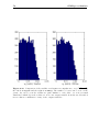
9.2 Monte Carlo results . . . . . . . . . . . . . . . . . . . . . . . . . .
9.3 Further work . . . . . . . . . . . . . . . . . . . . . . . . . . . . . .
69
69
74
79
10 Conclusions
81
Bibliography
83
A Quaternions
A.1 Basic definitions . . . . . . . . . . . . .
A.2 Translation . . . . . . . . . . . . . . . .
A.3 Rotation . . . . . . . . . . . . . . . . . .
A.4 Euler rotation expressed in quaternions
.
.
.
.
87
87
87
88
88
B User’s manual
B.1 Files . . . . . . . . . . . . . . . . . . . . . . . . . . . . . . . . . . .
B.2 Run OMSep . . . . . . . . . . . . . . . . . . . . . . . . . . . . . . .
89
89
90
C SepSim input data
95
Index
99
.
.
.
.
.
.
.
.
.
.
.
.
.
.
.
.
.
.
.
.
.
.
.
.
.
.
.
.
.
.
.
.
.
.
.
.
.
.
.
.
.
.
.
.
.
.
.
.
.
.
.
.
.
.
.
.
Chapter 1
Introduction
The purpose of this master’s thesis is to investigate if separation analysis can
be done using the program OpenModelica. The work is made at Saab Space
in Linköping and it is divided into two parts. The main part of the work is
to implement a mathematical model of a separation system in OpenModelica,
simulate it and study the behaviour of the system. The other part of the work is
to evaluate OpenModelica and compare it with other modeling programs, such as
Matlab/Simulink, C/C++ and JAVA to see advantages and disadvantages of the
programs.
1.1
Background
Saab Space develops and manufactures equipment for space. The main office is
located in Göteborg and they have a division in Linköping with two main products;
separation systems for launch vehicles and control systems for sounding rockets.
A separation system supports a satellite during ascent, releases the satellite upon
command and ejects the satellite from the launch vehicle. A sounding rocket is an
instrument-carrying rocket designed to take measurements and perform scientific
experiments in space.
Saab Space wants to investigate if the program OpenModelica [20], described
below, which uses the language Modelica can be used for modeling and simulation
of their separation systems. Modelica will maybe be a standard language for
modeling and therefore Saab Space wants to evaluate OpenModelica to see if this
is a program they can use.
OpenModelica is free software with the goal to create a complete Modelica
modeling, compilation and simulation environment based on free software. Modelica [18] is an object-oriented language for modeling and simulation of complex
physical systems. It has a JAVA and Matlab-like syntax. Modelica uses equationbased modeling, this means that the physical behaviour of a model is described
by differential, algebraic and discrete equations and no particular variable needs
to be solved manually.
1
2
Introduction
1.2
Problem description
When launching a satellite a separation system is used to keep the satellite attached
to a launch vehicle during ascent and to separate it from the launch vehicle while
in space. In separation analysis the separation is studied by simulations to see if
requirements on separation velocity and satellite angular velocity can be fulfilled.
To be able to simulate separations a mathematical model of the separation system
is needed. This model will be implemented in OpenModelica during the work with
this master’s thesis.
A Monte Carlo method will be used to get as reliable results as possible. When
using a Monte Carlo method the model will be simulated many times with some
small differences in the input data, this method randomly generates values for
uncertain parameters to simulate a model. This is done to make sure that the
system always will meet all its requirements.
To see if OpenModelica is suited for modeling this kind of systems it will be
evaluated and compared with other modeling programs, such as Matlab/Simulink,
JAVA and C/C++.
1.3
Purpose
The purpose of this master’s thesis is to
• Make a mathematical model of a separation system and implement it in
OpenModelica.
• Simulate the model to see if separation analysis can be performed.
• Use a Monte Carlo method when simulating the model.
• Evaluate OpenModelica and compare it with other modeling programs to
see advantages and disadvantages.
1.4
Disposition of the thesis
The structure of the thesis is described in this section.
Chapter 2, Launching satellites includes facts about satellites, adapters
and launch vehicles. These are the components needed for launching a satellite.
Chapter 3, Satellite separation describes the separation system.
Chapter 4, Modelica gives an introduction to the modeling language
Modelica and to the program OpenModelica.
Chapter 5, Model description describes the mathematical model of the
separation system and includes the equations.
1.4 Disposition of the thesis
3
Chapter 6, Monte Carlo describes Monte Carlo methods.
Chapter 7, OMSep implementation presents the implementation of OMSep,
the program developed in this master’s thesis.
Chapter 8, OpenModelica evaluation discusses advantages and
disadvantages with OpenModelica compared to other modeling programs, such
as Matlab/Simulink, JAVA, C/C++.
Chapter 9, OMSep evaluation compares the results from OMSep with the
results from SepSim, a corresponding program used at Saab Space now.
Chapter 10, Conclusions discusses the result of this master’s thesis.
Appendix A, Quaternions includes facts about quaternions.
Appendix B, User’s manual describes how to use the program OMSep.
Appendix C, SepSim input data describes the input files to the program
SepSim.
Chapter 2
Launching satellites
When launching a satellite, apart from the satellite, a launch vehicle and an
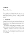
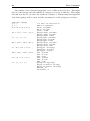
adapter are needed. These components are described below and can be seen in
Figure 2.1.
2.1
Satellite
A satellite is a smaller object that rotates around a larger object. Satellites that
have been placed into orbit by human are sometimes called artificial satellites to
distinguish them from natural satellites such as the moon. Most satellites orbit
the Earth. The satellites are designed for the missions they shall perform, such
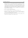
as weather satellites, communications satellites and navigation satellites. Weather
satellites, see Figure 2.2, observe atmospheric conditions over a large area to help
study weather patterns and forecasting the weather. A communications satellite,
see Figure 2.3, relays radio, television and other signals between points in space
and on Earth. Navigation satellites, see Figure 2.4, send signals that operators
of aircrafts, ships, land vehicles and people on foot can use to determine their
location. [16]
Satellites are also used to study the universe. Such satellites have orbited the
moon, the sun, asteroids, and the planets Venus, Mars, and Jupiter. These satellites mainly gather information about the bodies they orbit to help scientists to
investigate these bodies. Some examples of satellites and their weights, dimensions
and orbits can be seen in Table 2.1. [16]
2.1.1
Satellite orbits
Depending on the mission, satellite orbits have a variety of shapes. Some are
circular, while others are highly elliptical. Orbits also vary in altitude. For example
some circular orbits are just above the atmosphere at an altitude of about 250
kilometers, while others are about 36,000 kilometers above Earth. Many types of
orbits exist, but most artificial satellites that orbit Earth travel in one of three
types; geostationary earth orbit (geo), medium earth orbit (meo) and low earth
5
6
Launching satellites
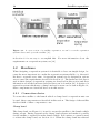
Figure 2.1. An example of a launch vehicle, Long March 3C, an adapter and a satellite.
The stages token together with the boosters are called a launch vehicle. A launch vehicle
and an adapter are used when launching a satellite. [22]
2.1 Satellite
7
Figure 2.2. This is a weather satellite, it observes atmospheric conditions over a large
area to help scientists study and forecast the weather. [16]
Figure 2.3. A communications satellite, such as Astra 1K shown here, relays radio,
television and other signals between points in space and on Earth. [16]
Mission
Communication
Navigation
Scientific
Example
Astra 1K [19]
Navstar GPS [8]
ENVISAT [7]
Weight [kg]
5250
1705
8211
Dimensions [m]
6.6 × 37.0
2.4 × 35.5
10.0 × 26.0
Table 2.1. Examples of satellites and their missions. The dimensions are satellite
height × wingspan. The numbers after the names of the satellites are the references to
the sources where more information about these satellites can be found.
8
Launching satellites
Figure 2.4. A navigation satellite, like this Global Positioning System (gps) satellite
sends signals that operators of aircraft, ships, land vehicles and people on foot can use
to determine their location. [16]
orbit (leo). Most orbits of these three types are circular. See [9, 16] for more
information about satellite orbits, these are the sources for this section.
geo satellites lie above the equator at an altitude of about 36,000 kilometers.
Communications satellites, which relays radio, television and other signals between
points in space and on Earth, are put into these high altitude orbits. The aim
with the geo is that it has a constant distance to the surface of Earth.
meo is the region of space around the Earth above leo and below geo. Radio
signals sent from a satellite at medium altitude can be received over a large area
of the surface of Earth. These orbits are stable and they have wide coverage which
makes them ideal for navigation satellites, such as gps satellites, see Figure 2.4.
A leo is just above Earth’s atmosphere, where there is still some air that
cause drag on the satellite and reduce its speed. Less energy is required to launch
a satellite into this type of orbit than into any other orbit. Satellites that point
toward deep space and provide scientific information generally operate in this
type of orbit. An example of a leo is the sun-synchronous polar orbit, it passes
almost directly over the North and South poles. A slow drift of the orbit position
is coordinated with Earth’s movement around the sun in such a way that the
satellite always crosses the equator at the same local time on Earth. Because the
satellite goes over all latitudes, its instruments can gather information on almost
the entire surface of Earth. These satellites can be used to study how natural
cycles and human activities affects the climate on Earth.
2.2 Adapter
9
Figure 2.5. This launch vehicle, Soyuz R-7A, was used to launch the world´s first
artificial satellite, Sputnik 1, on October 4 in 1957 [5].
2.1.2
Launched satellites
The Soviet Union launched the first artificial satellite, Sputnik 1, on October 4 in
1957. The launch vehicle used to launch this satellite, Soyuz R-7A, can be seen
in Figure 2.5. Since then, the United States and about 40 other countries have
developed, launched and operated satellites. Today, about 3,000 useful satellites
are orbiting Earth. Table 2.2 describes some examples of launch vehicles and which
nation and space agency they belong to. [16]
2.2
Adapter
An adapter is a physical structure used to connect a satellite to a launch vehicle,
some adapters that have been developed at Saab Space can be seen in Figure 2.6.
An adapter has a bolted launcher interface at the bottom and a satellite interface
at the top. The satellites can, as described in Section 2.1, have various of sizes
depending on their missions. The adapter makes it possible to use the same kind
of launch vehicle for all kinds of satellites. The adapter also includes a separation
system, described in Chapter 3, which is used to separate the satellite while in
space. [24]
2.3
Launch vehicle
A launch vehicle is a rocket used to carry a payload from the surface of Earth into
outer space. Usually the payload is a satellite which is placed into orbit. A launch
vehicle can be seen in Figure 2.1. There are various types of launch vehicles and
there are various ways to characterize them, for example if they are expandable or
reusable, by the amount of mass they can lift into orbit or the number of stages
10
Launching satellites
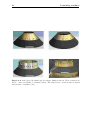
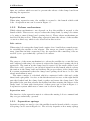
Figure 2.6. Saab Space Modular Payload adapter family is shown. These adapters are
used to connect a satellite to a launch vehicle. The adapters are of various sizes to match
various sizes of satellites. [24]
2.3 Launch vehicle
11
they employ, by nation or space agency responsible for the launch, this is described
in this section. To read more about launch vehicles see [9] which is the source for
this section.
2.3.1
Expandable and reusable
Expandable launch vehicles are designed to be used only once and their components are not recovered after the launch. These launch vehicles usually separate
from their payload and break up during atmospheric reentry. Reusable launch
vehicles, on the other hand, are designed to be recovered intact and used again for
subsequent launches. Most launch vehicles for launching satellites are expandable,
the only example of a reusable launch vehicle in operations is Nasa’s Space Shuttle which can be seen in Figure 2.7. This is the spacecraft currently used by the
United States government for its human spaceflight missions. It carries astronauts
and payload such as satellites or space station parts into low earth orbit. Usually
five to seven astronauts ride in the spacecraft. The weight and height of the Space
Shuttle can be seen in Table 2.2.
2.3.2
Mass and stages
Launch vehicles are often characterized by the amount of mass they can lift into
orbit or the number of stages they employ. A stage is mounted on top of or attached
next to another stage. The result is effectively two or more rockets stacked on top
of or attached next to each other. Taken together these are called a launch vehicle,
see Figure 2.1.
Each stage contains its own engines and fuel. By jettisoning stages when they
run out of fuel, the mass of the remaining rocket is decreased. This staging allows
the thrust of the remaining stages to more easily accelerate the rocket to its final
speed and altitude. Two stage rockets are quite common, but rockets with as many
as five separate stages have been successfully launched.
The main reason for multi-stage launch vehicles is that once the fuel is burnt,
the space and structure which contained the fuel and the motors themselves are
useless and only add weight to the vehicle which slows down its future acceleration.
By dropping the stages which are no longer useful, the rocket gets lighter. The
thrust of the future stages is able to provide more acceleration than if the earlier
stages were still attached, or than a single, large rocket would be capable of. When
a stage drops off, the rest of the rocket is still traveling near to the speed that
the whole assembly reached at burn-out time. This means that it needs less total
fuel to reach a given velocity and/or altitude. A further advantage is that each
stage can use its own type of rocket motor, with each stage/motor tuned for the
conditions in which it will operate.
On the downside, staging requires the vehicle to lift motors which are not being
used until later and makes the entire rocket more complex and harder to build.
But the savings are so great that every rocket currently used to deliver a payload
into orbit uses staging.
12
Launching satellites
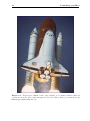
Figure 2.7. Nasa’s space shuttle is the only example of a reusable launch vehicle in
operations, it is the spacecraft currently used by the United States government for its
human spaceflight missions. [16]
2.3 Launch vehicle
2.3.3
13
Nation and space agency
Launch vehicles are also characterized by nation or space agency responsible for
the launch and the company that manufactures and launches the vehicle. Some
examples of launch vehicles, their nations, space agencies, weight, height and how
many stages they employ can be seen in Table 2.2.
Launch Vehicle
Space Shuttle [16]
Soyuz 2 [5]
Ariane 5 [7]
H-IIA(H2A) [12]
GSLV [11]
Long March 4B [4]
Shavit 2 [10]
Dnepr [28]
VSL [23]
Nation/
nations
USA
Russia
Europe
Japan
India
China
Israel
Ukraine
Brazil
Company/
agency
NASA
RSA
ESA
JAXA
ISRO
CALT
ISA
Yuzhmash
AEB
Weight
[103 kg]
2,029
305
777
285
402
254
0.25
211
1,4
Height [m]
Stages
58.12
46,1
59
53
49
44.1
3.76
34.3
8.0
2
2 or 3
2
2
3
3
2
3
2
Table 2.2. Examples of launch vehicles from various nations and space agencies. The
numbers after the names of the launch vehicles are the references to the sources where
more information about these launch vehicles can be found.
14
Launching satellites
2.4
Flight sequence during launch
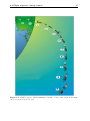
Figure 2.8 describes the flight sequence when launching a satellite, in this case
for the launch vehicle LM-3C [22] which can be seen in Figure 2.1. The first step
is the lift-off of the launch vehicle. Then the boosters and a bit later the first
stage will be separated from the rest of the launch vehicle. The boosters are used
to assist with the lift-off and these are sometimes referred to as stage 0. The
boosters and the stages separate when they have run out of fuel because then they
are no longer useful and the rocket gets lighter, to read more about how this works
see Section 2.3.2. The fairing it is used to protect the satellite while in Earth’s
atmosphere, this is no longer needed when outside the atmosphere and the launch
vehicle will therefor jettison the fairing then. After this has happened the third
stage will be separated. The last thing that will happen is that the satellite will
separate from the launch vehicle. To perform this separation a separation system,
described in Chapter 3, will give the satellite the needed velocity and angular rate
to be ejected from the launch vehicle. The following are a description of the steps
in the flight sequence which can be seen in Figure 2.8 (the numbers in the list
refers to the numbers in the Figure). [22]
1. Lift off
2. Pitch over
3. Booster separation
4. First/second stage separation
5. Fairing jettison
6. Second/third stage separation
7. Third stage first powered phase
8. Third stage coast phase
9. Third stage second powered phase
10. Attitude Adjustment
11. Satellite/launch vehicle separation
2.4 Flight sequence during launch
15
Figure 2.8. Flight sequence when launching a satellite. A list of the steps in the figure
can be seen in Section 2.4. [22]
Chapter 3
Satellite separation
When launching a satellite, see Chapter 2, it is important that the satellite is
secured to the launch vehicle during ascent and that the satellite separates while
in space. A connection device is needed to secure the satellite to the launch vehicle
and a release mechanism is needed to be able to separate the satellite. When the
satellite has been released it has to be ejected from the launch vehicle and be
given the provided kinetic energy. The system used to perform all this are called a
separation system. In Figure 3.1 a satellite separation can be seen and a separation
system can be seen in Figure 3.4. [24]
The requirements on a separation system and the hardware Saab Space uses in
their separation system are described in this chapter. To see if the requirements
are fulfilled separation analysis is done, this is also discussed here.
3.1
Requirements
A separation system has some requirements that have to be fulfilled, which depends
on the mission. The most important requirement is that the separation occur in
a controlled way. There are also requirements on the separation velocity and the
angular rate to make sure that the satellite will be placed into orbit.
Other requirements on the system are that it has to be able to attach the
satellite to a launch vehicle during ascent and that the satellite can be released
and ejected with the provided energy to be able to be placed into orbit while in
space.
A satellite separation is an abrupt course of events and when the satellite
separates it causes a mechanical shock to the satellite. Sometimes there are such
requirements on the system that this shock has to be low. To meet this requirement
a clamp band opening device (cbod), see Section 3.2.2, has been developed. Another requirement is that housekeeping data has to be transmitted to the ground
during ascent. This data is information about the satellite and its health and
safety.
The design of the system has to be made in such a way that it meets all the
requirements on the system. The design used at Saab Space which is described
17
18
Satellite separation
Figure 3.1. A cross section of a satellite separation, as can be seen the separation
system releases and ejects the satellite. [15]
in Section 3.2 is one way to accomplish this. For more information about the
requirements on a separation system, see [24]
3.2
Hardware
When designing a separation system it is desirable to have an simple design, because the most important is to make the separation system reliable, i.e. the satellite has to separate every time. A separation system can be designed in various
ways to meet the requirements described in Section 3.1. The hardware Saab Space
uses in their designs of separation systems are described in this section and more
information about the hardware described here can be found in [24]. A design of a
separation system which uses a clamp band and a cbod can be seen in Figure 3.4,
these components are described later on in this section.
3.2.1
Connection device
To secure the satellite to the launch vehicle a clamp band or separation nuts can
be used, these components are described in this section. The design of the satellite
decides which of these components to use.
Clamp band
The clamp band, see Figure 3.2, is used to secure the satellite to the launch vehicle
during ascent. During separation the clamp band releases and makes it possible
for the satellite to separate from the launch vehicle. Bolt cutters or a cbod is used
to release the clamp band, see Section 3.2.2. When the clamp band has released
3.2 Hardware
19
there are catchers which are used to prevent the release of the clamp band from
affecting the separation.
Separation nuts
When using separation nuts, the satellite is secured to the launch vehicle with
bolts. A separation nut can be seen in Figure 3.5.
3.2.2
Release mechanisms
Which release mechanism to use depends on how the satellite is secured to the
launch vehicle. There are two ways to release the clamp band; by using bolt cutters
or by using a cbod (clamp band opening device). These release mechanisms are
described in this section. When using separation nuts the release of the satellite
occurs in a third way, which is also described in this section.
Bolt cutters
When using bolt cutters the clamp band consists of two band halves, named straps,
for attaching the satellite to the adapter. The straps are joined together by two
strap joints that include connecting bolts. At separation the connecting bolts are
severed by two pyrotechnically operated bolt cutters.
CBOD
The purpose of the cbod mechanism is to release the satellite in a controlled way
and compared with using bolt cutters it reduces the clamp band opening shock at
separation. The tension in the clamp band is reacted by the cbod when closed.
This device will, operated by an electrical signal from the launch vehicle, release
the tension in the clamp band and facilitate the proper release of the clamp band.
If a system requirement is that the clamp band opening shock has to be low, this
release mechanism is used.
The cbod consists of a flywheel which is constructed with a left and a right
thread and a pin-puller. A screw on the left thread and a screw on the right thread
puts the flywheel and the clamp band together and tenses the clamp band. The
pin-puller is the part that releases the flywheel and thus starting the release of the
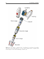
clamp band. A cbod with descriptions of these parts can be seen in Figure 3.3.
A separation system which uses a cbod can be seen in Figure 3.4.
Separation nuts
The function of the separation nuts is to release the mating bolt at command and
they are pyrotechnically operated.
3.2.3
Separation springs
Separation springs are used to eject the satellite from the launch vehicle, a separation spring can be seen in Figure 3.6. The velocity depends on how many springs
20
Satellite separation
Figure 3.2. A clamp band is used to secure a satellite to a launch vehicle during ascent,
the cbod is a release mechanism, it is used to release the clamp band at separation, and
the catchers catch the clamp band when it has released. [24]
3.2 Hardware
21
Figure 3.3. A cbod (clamp band opening device) is a release mechanism which is used
to reduce the clamp band opening shock at separation. [24]
22
Satellite separation
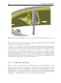
Figure 3.4. This separation system which uses a clamp band and a cbod is developed
at Saab Space.
3.2 Hardware
23
Figure 3.5. The function of the separation nuts is to release the mating bolt at command
and they are pyrotechnically operated. [24]
24
Satellite separation
Figure 3.6. Separation springs are used to eject the satellite from the launch vehicle. [24]
that are used and how much energy they employ. The angular rate of the satellite
depends on how the springs are placed.
There are two types of separation; symmetric separation, where the separation
springs do not contribute to the satellite rotation after separation, and asymmetric
separation, where the separation springs gives contribution to the satellite rotation
after separation. The symmetric separation is to prefer if no satellite rotation
caused by the separation is wanted. But if a certain angular rate on the satellite is
wanted the asymmetric separation can be used to achieve this. The springs sizes
and placements decides how the separation will occur and the requirements on the
system decides which type of separation will be used.
3.2.4
Umbilical connectors
During ascent it is required that housekeeping data can be transmitted to the
ground to make sure that everything is working properly. This is performed by
using umbilical connectors, an umbilical connector can be seen in Figure 3.7. The
umbilical connectors are not needed to be able separate the satellite but they give
a disturbance to the separation and how they affect the separation are described
in Chapter 5. Therefore they are a part of the separation system.
3.2 Hardware
25
Figure 3.7. Umbilical connectors are used to transmit housekeeping data to the ground.
This data is information about the satellite and its health and safety. [24]
26
3.3
Satellite separation
Separation analysis
In separation analysis the separation is simulated to see if requirements on separation velocity and satellite angular rate are fulfilled. This is done to determine if
the satellite will be placed into the wanted orbit. Separation springs are used to
achieve this velocity and this angular rate. The amount of energy for the springs,
the numbers of springs and how the springs are placed decides the separation velocity and angular rate. Which springs to use and where to place them to meet
the requirements on satellite velocity and angular rate can be analysed to find a
design that can be used in the real system. [25]
The separation analysis is done to verify that the chosen design fulfil all the
requirements on the system and that it can be used, see Section 3.1 for a description
of the system requirements. To make the analysis reliable it has to comprise all
uncertainties that can affect the system variables. To do this in an efficient way,
Monte Carlo simulations, see Chapter 6, are used. [25]
3.3.1
Release and ejection
A separation analysis covers two phases; release and ejection. The release phase
is defined to be the phase when the satellite and the launch vehicle have contact
through the separation plane. The duration of this phase normally is in the magnitude of a millisecond. In this phase it is studied how the release mechanism
affects the separation. [25]
The ejection phase comprises the time from the contact in the separation plane
has ceased until all of the separation springs have lost contact with the satellite
surface. The duration of this phase normally is in the magnitude of a few tenths
of a second. In this phase it is studied how the springs and umbilical connectors
affect the separation. [25]
3.3.2
Collision analysis
Sometimes also collision analysis is performed. This is to make sure that the
satellite will not collide with the launch vehicle when they separate. In this analysis
the points on the satellite and the points on the launch vehicle which are most
possible to collide are studied with simulations to see if the satellite and the launch
vehicle will collide. [25]
Chapter 4
Modelica
This chapter gives an introduction to Modelica [18], which is an object-oriented
language for modeling of complex physical systems. The aim is to construct a
standard language for describing physical models. Modelica is suited for multidomain modeling, for example modeling of mechatronic systems within automotive
and robotics applications. Such systems are composed of mechanical, electrical and
hydraulic subsystems, as well as control systems. Modelica uses equation-based
modeling, the physical behaviour of a model is described by differential, algebraic
and discrete equations. This means that the equations can be written as they are
with no need to manipulate them. [18]
There are two important differences between Modelica and other object-oriented
programming languages, such as C/C++ or JAVA; Modelica is a modeling language rather than a true programming language and the primary content of the
classes is a set of equations and not statements or blocks with assignments as in
other object-oriented programming languages. The equations do not describe assignment but equality. In contrast to a typical assignment statement, such as
x := 3y + 5;
(4.1)
where the left-hand side of the statement is assigned a value calculated from the
expression on the right-hand side, an equation may have expressions on both its
right- and left-hand sides, for example,
2x + y = 7z + w;
(4.2)
The Modelica language is acausal, i.e. the equations have no pre-defined causality.
This means that the user do not have to define which variables are inputs and
which are outputs in contrast to for example Simulink where the input-output
causality is fixed. In Modelica the simulation engine must manipulate the equations symbolically to determine their order of execution to solve the equation
system. [18]
27
28
4.1
Modelica
OpenModelica
OpenModelica [20] is a free software implementation of the Modelica language
and it is a project at Linköpings universitet. The goal is to create a complete
Modelica modeling, compilation and simulation environment based on free software distributed in source code form or binary form. OpenModelica is intended
for research, teaching and industrial usage. It is also used to experiment with
new language features and language design for the ongoing development of the
Modelica language. [20]
OpenModelica is written in a language called RML (Relational Meta Language). This language is based on natural semantics which is a popular formalism
for describing the semantics for compilers. By using the RML language this formalism is combined with efficient compilation into optimized C code. [1]
The OpenModelica environment consist of a compiler that translates Modelica
code into flat Modelica, which basically is the set of equations, algorithms and
variables needed to simulate the compiled Modelica model. The environment also
includes a shell, i.e. an interactive command and expression interpreter, similar to
a Matlab prompt, where models can be entered, computations can be performed
and functions can be called. In this environment it is also possible to execute
Modelica scripts, i.e. Modelica functions or expressions executed interactively or
a set of algorithm statements defined in a text file. [1]
4.2
Modeling with Modelica
Commercial software products such as MathModelica and Dymola have been developed for modeling with Modelica. It is also an open source project, the OpenModelica Project [20]. These programs have open model libraries which means that
the users are free to create their own libraries or modify the already made libraries.
This is to better match the users unique modeling and simulation needs. All programs that use the Modelica language can use the Modelica Standard Library,
described in Section 4.3. Both MathModelica and Dymola have an interactive
graphical environment. They also have some additional libraries in the various
application areas, such as biochemical, magnetic and vehicle dynamics libraries.
To see which additional libraries exist in MathModelica, see [13], and to see which
additional libraries exist in Dymola, see [6].
4.2.1
Models
Modelica models consists of several smaller sub models which can be joined together to form larger and more advanced models. The models are built as classes,
and functions can be used to facilitate the evaluations. In Modelica everything
is described using classes, it is the only way to build abstractions and it enables
structured modeling. [18]
4.2 Modeling with Modelica
29
Classes
A class contains variable declarations, an algorithm section with assignments and
an equation section describing the behaviour of the class. Similar classes have a
base class with the common properties which they inherit from. The syntax of a
class can be seen below, where “name” is the name of the class. [18]
class name
variable declarations;
algorithm
algorithm section;
equation
equation section;
end name;
Functions
A number of mathematical functions like abs, sqrt, mod, etc. are predefined in
the Modelica language whereas others such as sin, cos, exp, etc. are available in
the Modelica standard mathematical library Modelica.Math. See Section 4.3 for
a description of the Modelica libraries. User-defined functions can also be useful
when modeling. [18]
Modelica functions are mathematical functions with no memory, they always
return the same results given the same arguments. The syntax of a function
definition (where name is the name of the function) can be seen below and it
is quite close to the syntax of a class definition. The body of a function is an
algorithm section that contains algorithmic code to be executed when the function
is called. Input and output parameters are also defined in the function. [18]
function name
input declarations;
output declarations;
algorithm
algorithm section;
end name;
4.2.2
Formulation of equations
To help Modelica solve an equation system and to give the right solution it is
important how the equations are formulated. But the most important is that the
number of equations is equal to the number of variables. Some aspects about
formulating the equations are described in this section. [18]
Division by zero and square roots
During a simulation a lot of problems that stop the solving process can occur.
One problem is division by zero. Formulations involving square roots could be
another problem, because the square root function is returning complex numbers
30
Modelica
for negative values. This is a problem if no complex numbers are wanted in the
model. It is important to reformulate the equations in a way that these problems
will not occur.
Initial values
When Modelica solves an equation system each variable has the default initial
value zero. To increase the probability to find a solution, and to do it in a more
efficient way, it is possible to set a more appropriate initial value. To find the
solution fast, it is important to have a good initial value of as many variables as
possible in the model. In some equations initial values have to be set to get the
right solution. For example the differential equation
ẋ = ax
(4.3)
where a is a constant will result in the solution x = 0 if no initial value is set to
x. If the wanted solution instead is
x = eat
(4.4)
then the initial value of x has to be set to 1.
If-statements
When using if-statements it is important that the number of equations in the ifpart is equal to the number of equations in the else-part. Because if this is not
true the number of equations will not be equal to the number of variables. An
example of this is the two if-statements below which will produce the same result.
The first is is written with equations as in Modelica.
class if-example
Real a(start=0);
Real b;
equation
if time > 0.1 then
a = 1;
b = 2;
else
a = 0;
b = 1;
end if;
end if-example;
The second is written with assignments as in other programming languages such
as C/C++ or JAVA.
4.3 Modelica libraries
31
class if-example
Real a(start=0);
Real b;
algorithm
if time > 0.1 then
a := 1;
b := 2;
else
b := 1;
end if;
end if-example;
Real a(start=0) gives a the initial value 0 in both examples. In the second ifstatement a will have the initial value 0 as long as the if-statement is false. But
in the first if-statement an equation is needed to perform this, because otherwise
the number of equation will not be the same as the number of variables.
4.3
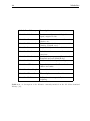
Modelica libraries
In Modelica related classes in particular areas are grouped into packages to make
them easier to find. Modelica Standard Library [17] is a standardized, predefined package. It provides constants, types and model classes of components from
various application areas, which are grouped into sub packages of the Modelica
Standard Library package. The currently available libraries in Modelica Standard
Library can be seen in Table 4.1. The libraries in Modelica Standard Library can
be used in OpenModelica, accept from Mechanics.MultiBody library and Media library, which are not implemented in OpenModelica yet. The libraries can be used
freely for both commercial and noncommercial purposes. Additional libraries are
available in application areas such as thermodynamics, hydraulics, power systems,
data communication, etc. The full documentation as well as the source code of
these libraries appear at the Modelica web site [18]. The most of these additional
libraries are implemented in OpenModelica. There are also some libraries for commercial usage, such as libraries for vehicle dynamics, hydraulic components and
air conditioning systems. [17]
Because OpenModelica has open source code everyone can develop new libraries
both for personal usage and to share with others. This means that the Modelica
libraries are growing all the time.
4.3.1
Add a new Modelica library
To build a model in OpenModelica the easiest way is to first find out if some of
the functions needed for the modeling already exist in the available libraries. If
some of the libraries can be used, then add these libraries and use the functions.
To add a new Modelica library and to be able to use the functions in the library
the following has to be done.
32
Modelica
Modelica Library
Description
Modelica.Blocks
Continuous, discrete and logical
input/output blocks.
Common constants from mathematics,
physics, etc.
Common electrical component models
(Analog, Digital, etc.).
Graphical layout of icon definitions.
Modelica.Constants
Modelica.Electrical
Modelica.Icons
Modelica.Math
Modelica.Mechanics
Modelica.Media
Modelica.SIUnits
Definitions of common mathematical
functions.
Mechanical components (Rotational,
Translational and MultiBody)
Media models for liquids and gases.
Modelica.StateGraph
Type definitions with SI standard
names and units.
Hierarchical state machines.
Modelica.Thermal
Thermal phenomena, heat flow, etc.
Modelica.Utilities
Utility functions especially for
scripting.
Table 4.1. A description of the libraries currently included in the Modelica Standard
Library. [17]
4.3 Modelica libraries
33
• Open the source code for the packages (.mo files) in the library and delete
extends Icon.Library and extends Icon.Library2 everywhere in the code.
Icon.Library and Icon.Library2 are used for the graphical interface of the
Modelica language and they makes icons for the libraries (extends Icon.Library
and extends Icon.Library2 should not be deleted if a graphical editor is used).
If these libraries are not removed from the code it will be errors when trying to simulate the packages, because if no graphical editor is used the icon
libraries will have no function.
• Use the command loadModel(Modelica).
• Use the command loadFile for each package (.mo-files) to use.
• Simulate the packages. These packages are exactly as all other .mo-files, i.e.
they have to be simulated before they can be used, otherwise the functions
do not exist in the OpenModelica environment.
• The functions in the packages can now be used. In the packages every
function has a description of how it shall be used.
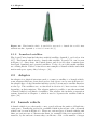
Chapter 5
Model description
The separation system model which has been developed in this master’s thesis
describes two rigid bodies which separates from each other. The two bodies are a
satellite and a launch vehicle which are both modeled with six degrees of freedom,
often denoted as 6DoF. 6DoF refers to motion in three dimensional space combined
with rotation about three perpendicular axes. In this Chapter the equations used
in the model and the theory behind them are described. To read more about the
model equations used in this Chapter, see [26].
5.1
Theory
The theory behind the equations used in the separation system model, i.e. the
theory of how forces and torques act on rigid bodies, is described in this section.
5.1.1
Newton’s laws of motion
When having rigid bodies Newton’s second and third laws of motion are used to
calculate the forces acting on the bodies and the movements of the bodies. These
laws are described in this section.
Newton’s second law of motion
Newton’s second law of motion tells that the net force on a particle is proportional
to the time rate of change of its linear momentum (linear momentum is the product of mass and velocity)
X
F
=
d(mv)
dt
(5.1)
where F is the force acting on the particle, m is the mass of the particle and v is
35
36
Model description
Figure 5.1. An illustration of Newton’s third law of motions.
the velocity of the particle. This law is often stated as
X
F = ma
(5.2)
where a is the acceleration of the particle. [21]
Newton’s third law of motion
Newton’s third law of motion tells that whenever a particle, A, exerts a force on
another particle, B, B simultaneously exerts a force on A with the same magnitude
in the opposite direction. This together with Newton’s second law of motion gives
the following equations for a system of two rigid bodies, A and B
F
= mA aA
(5.3)
−F
= mB aB
(5.4)
where mA and mB are the masses of particle A respective particle B and aA and
aB are the accelerations of particle A respective particle B. An illustration of this
can be seen in Figure 5.1. [21]
5.1.2
Torque
If a force is applied to a body and the force point of support is not the center of
gravity of the body, the force will cause a torque to the body. For a rigid body
this torque is calculated as the cross product
5.2 Coordinate systems
37
M
= r×F
(5.5)
where M is the torque, r is the position of the force point of support relative the
center of gravity of the body and F is the force acting on the body. [21]
If a torque is acting on a rigid body this will cause an angular rotation of the
body. The relation between the torque and the angular rotation of the body is
described as
X
M
= Iα
(5.6)
where M is the torque, I is the moment of inertia and α is the angular acceleration.
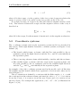
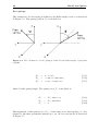
5.2
Coordinate systems
The coordinate systems used in the separation system model are described in
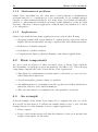
this section. Three right-handed Cartesian coordinate systems, see Figure 5.2 are
defined. [26]
• The launch vehicle frame, lv-frame, with the XLV -axis parallel to the lv
symmetry axis in the flight direction and the YLV - and ZLV -axis initially in
the separation plane.
• The not moving reference frame which initially coincides with the lv-frame.
• The satellite frame, sc-frame with the origin in the separation plane, the
XSC -axis parallel to the sc symmetry axis in the satellite flight direction
and the YSC - and ZSC -axis initially in the separation plane.
An example of how the coordinate systems used in the model can look like after
the satellite and the launch vehicle have separated a bit from each other can be
seen in Figure 5.3
The sc orientation is defined by rotations with the Euler angles; φ, θ, ψ with
the rotations from the reference frame performed in order ψ, θ, φ. ψ is rotation
about the Y-axis, θ is rotation about the new X-axis and φ is rotation about
the new Z-axis. For example the application [−90◦ , −45◦ , −90◦ ] is illustrated in
Figure 5.4. [26]
38
Model description
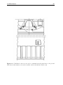
Figure 5.2. Right-handed Cartesian coordinate system, this is how the three coordinate
systems used in the model initially will look like. [26]
Figure 5.3. An example of how the coordinate systems used in the model can look like
after the satellite and the launch vehicle have separated a bit from each other.
5.2 Coordinate systems
39
Figure 5.4. Rotation from the reference frame to the sc frame with the Euler angles
φ, θ, ψ performed in order ψ, θ, φ. ψ is rotation about the Y-axis, θ is rotation about the
new X-axis and φ is rotation about the new Z-axis. The application [−90◦ , −45◦ , −90◦ ]
is illustrated in this Figure. [26]
40
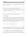
5.3
Model description
Velocity and position
This section describes the equations used in the separation system model to calculate the satellite and launch vehicle velocity and position.
The satellite and the launch vehicle can be described as two rigid bodies. Therefore Newton’s second and third laws of motion, see 5.1.1, is used to calculate the
velocity and the position of the satellite and the launch vehicle. If the separation is
asymmetric, see Section 3.2.3, the satellite and the launch vehicle will get angular
rates when they separate from each other. Newtons second law of motion gives
the following equations
Fnet
=
ma + ω × mv
(5.7)
v̇
=
a
(5.8)
ṗ
=
v
(5.9)
where the term ω × mv in equation 5.7 describes the satellite and launch vehicle rotation in the sc frame respective the lv frame relative to the reference
frame. The acceleration, a = (ax , ay , az ), the velocity, v = (vx , vy , vz ), the angular rate, ω = (ωx , ωy , ωz), the position, p = (px , py , pz ) and the total force,
Fnet = Fnetx , Fnety , Fnetz , are defined in the sc-/lv-frame.
Fnet is the net force acting on the body, i.e. the vector sum of all the forces
acting on the body. Only the springs and the umbilical connectors, which are
described later on in this chapter, will cause forces on the bodies, therefore
Fnet
=
Fs1 + Fs2 + ... + Fsn + Fuc1 + Fuc2 + ... + Fucm
(5.10)
where Fs1 , Fs2 , ..., Fsn are the forces caused by the n springs used in the model
and Fuc1 , Fuc2 , ..., Fucm are the forces caused by the m umbilical connectors used
in the model.
Newton’s third law of motion, see Section 5.1.1, can be used to calculate the
velocity and the position of the satellite and of the launch vehicle because the
satellite and the launch vehicle are modeled as two rigid bodies. This law tells
that if a force F acts on the satellite then a force -F will act on the launch vehicle,
which gives the following equations for the satellite
Fnet
= msc asc + ωsc × msc vsc
(5.11)
v̇sc
=
asc
(5.12)
ṗsc
=
vsc
(5.13)
and the following equations for the launch vehicle
−Fnet
=
mlv alv + ωlv × mlv vlv
(5.14)
v̇lv
=
alv
(5.15)
ṗlv
=
vlv
(5.16)
5.4 Torque
41
To calculate the relative separation velocity between the satellite and the launch
vehicle, vrel , the velocities vsc and vlv has to be transformed to the reference frame.
Then vrel is calculated as
vrel
=
vsc0 − vlv0
(5.17)
where vsc0 is the satellite velocity transformed to the reference frame and vlv0 is
the launch vehicle velocity transformed to the reference frame.
The distance, d, between the satellite and the launch vehicle is calculated in
the same way, the positions psc and plv has to be transformed to the reference
frame and then d is calculated as
d =
psc0 − plv0
(5.18)
where psc0 is the satellite position transformed to the reference frame and plv0 is
the launch vehicle position transformed to the reference frame.
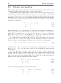
5.4
Torque
The forces acting on the bodies are provided by springs and umbilical connectors, which are described later on in this chapter. If the placement of the springs
and/or the umbilical connectors have any asymmetry, such as the amount of energy of the springs/umbilical connectors differ or the center of gravity of the body
is not placed in origo of the reference frame, they will cause torques on the bodies,
see Section 5.1.2. The torque is modeled in the same way for the springs and the
umbilical connectors, which gives the following cross product
Ms = Sp × Fs
(5.19)
for each of the springs and the following cross product
Mu = Up × Fu
(5.20)
for each of the umbilical connectors, where Ms = Msx , Msy , Msz is the torque
caused by the spring, Mu = Mux , Muy , Muz is the torque caused by the umbilical
connector, Sp is the spring position, Up is the umbilical connector position and
Fs /Fu is the force acting on the body caused by the spring/umbilical connector.
5.5
Angular rate and orientation quaternion
If a torque, see Section 5.1.2, is acting on the system, the satellite and the launch
vehicle will get angular rates, the following equation is used to calculate the angular
42
Model description
rate and this equation can be used both for the satellite and for the launch vehicle.
Mnet
=
Iα + ω × (Iω)
(5.21)
ω̇
=
α
(5.22)
where the term ω × (Iω) describes the satellite and launch vehicle rotation in the
sc frame respective the lv frame relative to the reference frame. The the vector
sum of all the torques acting on the satellite/launch vehicle, Mnet , the angular
acceleration, α, and the angular rate, ω, are defined in the sc-/lv-frame. The
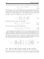
moments of inertia, I, are defined by moment of inertia tensors

I
=

−Ixz
−Iyz 
Izz
−Ixy
Iyy
−Iyz
Ixx
 −Ixy
−Ixz
(5.23)
This gives the following equation for the satellite
Mnetsc αsc
ω̇sc
=
Isc + ωsc × (Isc ωsc )
(5.24)
= αsc
(5.25)
and the following equation for the launch vehicle
Mnetlv αlv
ω̇lv
= Ilv + ωlv × (Ilv ωlv )
(5.26)
= αlv
(5.27)
The torque will cause an angular rotation of the satellite/launch vehicle, this
rotation is defined by quaternions, Q = (q0 , q1 , q2 , q3 ), see Appendix A for a description of quaternions. The quaternions describe the relation between the sc/lv
frame and the reference frame and they are used to transform between the frames.
The following algorithm is used to calculate the orientation quaternion, Q, and
this algorithm can be used both to calculate the satellite orientation quaternion,
Qsc and to calculate the launch vehicle orientation quaternion, Qlv


0
q̇0
 q̇1  1  ω1
 = 
 q̇2  2  ω2
ω3
q̇3

Q̇ =
5.6
−ω1
0
−ω3
ω2
−ω2
ω3
0
−ω1

−ω3
−ω2 

ω1 
ω0


q0
 q1 
 
 q2 
q3
(5.28)
Forces and torques acting on the system
The forces and torques acting on the bodies are provided by springs and umbilical
connectors, see Section 3.2.3 respective 3.2.4. There are two kinds of springs; fixed
5.6 Forces and torques acting on the system
43
springs and free springs and the forces and torques that they produce are wanted
by the system. The umbilical connectors do not have the purpose to provide the
system with forces and torques, they can instead be seen as disturbances to the
system. But they affect the system in the same way as the springs and are therefore
modeled as the springs. These components are described later on in this section.
5.6.1
Spring local frame
A spring local frame, (XSP , YSP , ZSP ), is defined to describe the position of the
springs and the umbilical connectors. The spring top connection point to the
satellite is defined by the polar coordinates r and Φ and the distance above the
separation plane, h, expressed in the reference frame, (X0 , Y0 , Z0 ). The origin is
defined to be the spring attachment point to the launch vehicle. The spring local
frame and the reference frame can be seen in Figure 5.5 (h is assumed to be zero).
Figure 5.5. The reference frame (X0 , Y0 , Z0 ) for the separation system and a spring
local frame for the spring, (XSP , YSP , ZSP ) which is defined by the polar coordinates r
and Φ with origin in the spring attachment point to the launch vehicle.
5.6.2
Spring position and force
The input data to the model describes the position of the spring top connection
point to the satellite, the position of the spring local frame origin expressed in
the reference frame, Sp = (x, y, z), is needed to be able to determine the torque
caused by the spring. How to calculate Sp and the force, F , caused by the springs
44
Model description
depends on if it is a fixed spring, a free spring or an umbilical connector, this is
described in this section.
Fixed springs
When using fixed springs, the spring can tilt an angle α as described in Figure 5.6.
The spring position, Sp , is modeled as
Spx
= h − l cos α
(5.29)
Spy
= −r sin φ + l sin α
(5.30)
Spz
= r cos φ
(5.31)
where l is the spring length. The spring force, Fs , is modeled as
Figure 5.6. The orientation of a fixed spring is defined by the tilt angle α around the
Z-axis.
Fsx
=
Fstot cos α
(5.32)
Fsy
=
−Fstot sin α
(5.33)
Fsz
=
0
(5.34)
The magnitude of the spring force, Fstot , is defined by three parameters; initial
force, cut off force and stroke (the spring extension length) as defined in Figure 5.7.
5.6 Forces and torques acting on the system
45
Figure 5.7. The magnitude of the spring force, Fstot , is defined by three parameters;
initial force, cut off force and stroke.
46
Model description
Free springs
The orientation of a free spring is defined by the Euler angles θ and ψ as described
in Figure 5.8. The spring position, Sp , is modeled as
Figure 5.8. The orientation of a free spring is defined by the Euler angles ψ (left) and
θ (right).
Spx
=
h − l cos θ
Spy
=
−r sin φ + l sin θ sin ψ
(5.36)
Spz
=
r cos φ − l sin θ cos ψ
(5.37)
(5.35)
where l is the spring length. The spring force, Fs , is modeled as
Fsx
=
Fstot sin θ cos ψ
(5.38)
Fsy
=
Fstot sin θ sin ψ
(5.39)
Fsz
=
0
(5.40)
The magnitude of the spring force, Fstot , is the same as for fixed springs, i.e. it is
defined by the three parameters initial force, cut off force and stroke as described
in Figure 5.7.
5.6 Forces and torques acting on the system
47
Umbilical connector
The umbilical connector position, Up , is modeled as
Upx
=
h
(5.41)
U py
=
−r sin φ
(5.42)
U pz
=
r cos φ
(5.43)
The umbilical connector force, Fu , is modeled as
The magnitude of the
spring extension phase
eters; initial force, cut
stroke2 (pin retraction
Fux
=
Futot
(5.44)
Fuy
=
0
(5.45)
Fuz
=
0
(5.46)
umbilical connector force, Futot , consists of two parts; a
and a pin retraction phase. Futot is defined by five paramoff force, min force, stroke1 (spring extension phase) and
phase) as defined in Figure 5.9.
Figure 5.9. The magnitude of the umbilical connector force, Futot , is defined by five
parameters; initial force, cut off force, min force, stroke1 and stroke2.
48
5.6.3
Model description
Components which are not included in the model
This model only describes the forces caused by springs and umbilical connectors.
As described in Section 3 the separation system comprises some more components,
such as separation nuts or a clamp band with bolt cutters or with a cbod. The
springs used in the model can be extended, they can for example get parameters which describe the friction in the springs and parameters which describe the
deflection in the springs. Further work which can be done with the model is to
implement these components, to read more about further work, see Section 9.3.
Chapter 6
Monte Carlo methods
Monte Carlo methods are widely used for simulating the behavior of various physical and mathematical systems. They randomly generate values for unknown parameters to simulate models of the systems. The methods are distinguished from
other simulation methods by being stochastic, i.e. they are using random numbers or in practice, pseudo-random numbers. These randomly generated values
are often uniform or normal distributed.
Monte Carlo methods are based on the fact that the average value of a number
of independent observations gets closer and closer to the mean value as the number
of observations increases. This means that the result will be normal distributed
when using a Monte Carlo method. To read more about Monte Carlo methods,
see [3, 2] which are the sources in this chapter.
6.1
The use of Monte Carlo
Two common situations where Monte Carlo are used are when simulating physical
models and to find solutions to mathematical problems. These and some more
applications are discussed in this section.
6.1.1
Simulating physical models
When simulating physical models it is important to do many simulations with some
small differences in the input data for the uncertain variables (if there are any) to
get as reliable results as possible. This is to make sure that the model always will
fulfil all its requirements. Monte Carlo simulation is a method to perform this, it
randomly generates values for uncertain variables to simulate a model.
In OMSep, the program developed in this master’s thesis, a Monte Carlo method
is used. This method randomly generates uniform distributed values for the uncertain parameters and simulates the model with these values. The implementation
of this Monte Carlo function is described in Section 7.4.
49
50
Monte Carlo methods
6.1.2
Mathematical problems
Monte Carlo algorithms are also often used to find solutions to mathematical
problems that are too complicated to solve analytically by for example integral
calculus or other numerical methods. For many types of problems, its efficiency
relative to other numerical methods increases as the dimension of the problem
increases. The most common application of the Monte Carlo method is to use it
to do integration.
6.1.3
Applications
Monte Carlo methods have many application areas, such as the following
• Studying systems with a large number of coupled degrees of freedom, such as
liquids, disordered materials, strongly coupled solids, and cellular structures.
• Evaluation of definite integrals.
• Calculation of risk in business.
• Computational physics, physical chemistry and related applied fields.
6.2
Basis components
As can be seen in Section 6.1 there are many types of Monte Carlo methods
and depending on application areas the methods can differ a bit. The following
components comprise the basis of most Monte Carlo applications.
• The physical or mathematical system must be described by a set of probability distribution functions.
• A random number generator must be available.
• An implementation for sampling from the specified probability distribution
functions with use of the random numbers.
• The outcomes must be accumulated into the quantities of interest.
6.3
An example
A trivial example of the Monte Carlo method is to estimate the area of a circle.
It is trivial because there is a well known formula which is easy to use, but this
example has most of the elements of more complex applications.
1. Draw a square.
2. Draw a circle in the square such that the diameter of the circle and the side
length of the square are the same.
6.4 Monte Carlo and random numbers
51
Figure 6.1. This figure illustrates an example of estimating the area of a circle with use
of a Monte Carlo method.
3. Randomly cover the surface of the square with dots, see Figure 6.1
4. Count all the dots, then count the ones inside the circle, the area of the circle
is then estimated as
Acircle (estimated)
=
Asquare ×
dotsinside
dotsall
(6.1)
By increasing the number of dots, the accuracy of the estimation will increase.
When
using Monte Carlo methods the accuracy of the estimation increases as
√
number of experiments.
6.4
Monte Carlo and random numbers
Monte Carlo simulation methods do not generally require truly random numbers
to be useful. Many of the most useful techniques use pseudo-random sequences,
described later on in this section, which makes it easy to test and re-run simulations. The only quality usually necessary to make good simulations is that
the pseudo-random sequence appear randomly enough. What this means depends
on the application, but typically the sequence should pass some statistical tests.
Testing that the numbers are uniformly distributed, normal distributed or follow
another desired distribution is the simplest and most common ones.
6.4.1
Pseudo-random numbers
A pseudo-random number is a number that appears random but is not truley random. Pseudo-random sequences typically have statistical randomness while being
generated by an entirely deterministic causal process. Such a process is easier to
produce than a genuine random one and it can be used again and again to produce exactly the same numbers. This is useful when testing software. There is
52
Monte Carlo methods
Figure 6.2. The probability density function for the uniform distribution U(a,b).
no known method to produce true randomness, because if any factor determines
the outcome it would mean that the produced number is not random at all. The
random number generation functions provided in all software packages are therefore pseudo-random, as for example the function randn in Matlab which produces
normally distributed random numbers.
6.4.2
Probability distributions
The randomly generated numbers used in Monte Carlo methods follows a probability distribution. The two most common used distributions, uniform distribution
and normal distribution, are described in this section.
Uniform distribution
Uniform distribution is a probability distribution such that each number on the
support of the distribution are equally probable. The support is defined by two
parameters, a and b, which are the minimum and maximum values of the support.
The distribution is often abbreviated U(a,b). The probability density function for
the uniform distribution U(a,b) is
f (x)
=
1
b−a
f or a ≤ x ≤ b, 0 else
(6.2)
(6.3)
and it can be also be seen in Figure 6.2.
6.5 Monte Carlo history
53
Figure 6.3. Probability density functions for some normal distributions with the mean,
µ, and the variance, σ.
Normal distribution
A normal distributed, also called the Gaussian distributed, variable is defined by
two parameters; mean (average value), µ, and variance (variability), σ. The distribution is often abbreviated N(µ, σ). The normal distribution is the most widely
used family of distributions in statistics. Many statistical tests are based on the
assumption of normality and if having enough numbers from some distribution, the
numbers will be asymptotically normal distributed. Probability density functions
for some normal distributions, N(µ, σ), can be seen in Figure 6.3.
6.5
Monte Carlo history
Monte Carlo methods were originally practiced under more generic names such as
statistical sampling. The name Monte Carlo is a reference to the famous casino in
Monaco, because the methods use of randomness and the repetitive nature of the
process are analogous to the activities at a casino.
Chapter 7
OMSep implementation
The program developed in this master’s thesis, OMSep (OpenModelica Separation),
consists of a model of a separation system, a function which gives input data to the
model, a function which simulates the model and a function which saves the output
data. An overview of OMSep can be seen in Figure 7.1 and the implementation of
the program is described in this chapter. A Monte Carlo method can also be used
when simulating the model, the implementation of the function to perform this is
also described in this chapter.
Figure 7.1. An overview of OMSep, the program developed in this master’s thesis. It
consists of a model of a separation system, a function which gives input data to the model,
a function which simulates the model and a function which saves the output data.
7.1
Input data
The input data to OMSep are written in the files Sep.Inp and Spring.Inp. In
Sep.Inp the satellite and launch vehicle input data are written and the spring
input data are written in Spring.Inp. Examples of input files and a description
of how to use them can be seen in Appendix B.
A Python script, readSepinput.py, is used to read the input data from the
input files. This script only reads the input data and saves them as variables.
55
56
7.2
OMSep implementation
Model implementation
The separation system model, see Chapter 5, is implemented in OpenModelica,
see Section 4.1, and it comprises a model of a satellite, a model of a launch vehicle
and a model of a separation system. These sub models are build as classes and
there are some functions to facilitate the evaluations, see Section 4.2.1. To get
the model structured the classes that have common properties share a base class
which they inherit from. The system is described below and a system overview
with the structure of the model classes and functions can be seen in Figure 7.2.
The model equations are described in Chapter 5.
Figure 7.2. An overview of the model classes and functions. Evaluate is the main class
where the calculations are done and CrossProduct, mm2m and QuatRot facilitates the evaluations. Evaluate have objects of the classes LaunchVehicle, SpaceCraft, FixedSpring,
FreeSpring and UmbilicalConnector. LaunchVehicle and SpaceCraft have a base class,
Body which they inherit from. FixedSpring, FreeSpring and UmbilicalConnector have
a base class, SpringModel, which they inherit from.
7.2 Model implementation
7.2.1
57
Functions
CrossProduct and mm2m are the only functions in Figure 7.2, all the others are
classes. CrossProduct calculates the cross product of two 3x1-vectors and mm2m
translates from millimeter to meter. It is also one function, Constants.D2R, from
the Modelica Standard Library, see Section 4.3, used in the model. This function translates from degrees to radians. The functions are used to facilitate the
calculations in the classes.
7.2.2
Classes
All the sub models of the model are described using classes, because in Modelica
everything is described using classes and it is the only way to build abstractions.
The model classes are described in this section.
Evaluate
There are a main class, Evaluate, where all the calculations which uses more than
one of the model classes are done. It uses all the other classes to calculate the
relative separation velocity between the launch vehicle and the satellite and the
satellite angular rate. This class brings all the sub models together to form a whole
model of a separation system.
QuatRot
The class QuatRot calculates quaternion rotation and the class Evaluate uses
this class for rotating between the reference frame and the other frames. For a
description of the frames, see Section 5.2, and for a description of quaternions, see
Appendix A.
Body
A satellite and a launch vehicle have many variables in common, such as mass,
moment of inertia, velocity and position, and therefore they have a base class,
Body, with the common properties which they inherit from.
SpringModel
Fixed springs, free springs and umbilical connectors also have many variables in
common, such as forces and orientation, and they have some calculations in common, such as computation of torques and forces. Therefore they have the base
class, SpringModel, which they inherit from. The class FixedSpring can be seen
on the next page, it illustrates the syntax of the classes.
58
OMSep implementation
class FixedSpring
"Includes variables and calculations for a fixed spring"
extends SpringModel;
Real alpha[NoS];
//Spring tilt angle (rad)
equation
if Spring == 0 then //Spring = 0 if there are no fixed springs
Ftot = {0};
Sposx = {0};
Sposy = {0};
Sposz = {0};
Fi = [0;0;0];
else
for i in 1:NoS loop
//Position of the spring, expressed in the reference frame
Sposx[i] = springh[i] - springl[i]*cos(alpha[i]);
Sposy[i] = -(SpringRadius[i]*cos(SpringPhi[i])
- springl[i]*sin(alpha[i]));
Sposz[i] = SpringRadius[i]*sin(SpringPhi[i]);
//Force caused by the spring expressed in the reference frame
Ftot[i] = if distance <= stroke[i] then
(Fmax[i] - ((Fmax[i]-Fmin[i])/stroke[i])*distance) else 0;
Fi[1,i] = Ftot[i]*cos(alpha[i]);
Fi[2,i] = -Ftot[i]*sin(alpha[i]);
Fi[3,i] = 0;
end for;
end if;
end FixedSpring;
7.3 Output data
7.2.3
59
Simulation of the model
To simulate the model a Python script, writeOMScript.py, is used. It assigns the
input data to the model variables and loads all the needed OpenModelica files, i.e.
all the classes and functions that the model consists of. This script also simulates
the model and saves the output variables.
7.3
Output data
The most important variables in the model are the relative separation velocity
between the satellite and the launch vehicle and the satellite angular rate, therefore
the output data consists of these variables.
The output data from OMSep consists of the values that the variables have in
each point of time during the simulation and it also consists of a time vector. A
Python script, sim.py, writes the output data to the Matlab file SepOutput.m.
This file can be run in Matlab and plots of the results can be performed to analyse
the result.
7.4
Monte Carlo implementation
OMSep also includes the possibility to use a Monte Carlo method, see Chapter 6 for
a description of Monte Carlo methods, when simulating the model. This section
describes how this function is implemented and an overview of the program which
includes the Monte Carlo function can be seen in Figure 7.3.
Figure 7.3. An overview of OMSep, when using a Monte Carlo method. It consists
of a model of a separation system, a function which gives input data to the model, a
function which performs a Monte Carlo method, a function which simulates the model
and a function which saves the output data.
The input data to the Monte Carlo function are written in the file MC.Inp.
For a description of how to use the input file, see Appendix B. When using
the Monte Carlo function the separation system model will be simulated a userdefined number of times. The variables which exist in the file MC.Inp will vary
from simulation to simulation and these variables are uniform distributed random
numbers. The maximum allowed variation in the parameters are set in the file
60
OMSep implementation
MC.Inp and the mean values of the variables are the values which have been set
in the input files Sep.Inp and Spring.Inp.
Two Python scripts are used to perform this; readMCinput.py and mc.py.
readMCinput.py reads the input data from the input file MC.Inp and saves them
as variables. readMCinput.py can be seen on the next page it illustrates the syntax
of the script files. The script mc.py produces uniform random numbers for the
variables in the file MC.Inp and writes the output data from the simulations to
file.
The output data from OMSep when using the Monte Carlo function consists of
the values that the variables have at the end time of each simulation, i.e. when
the separation has fulfilled and the satellite and the launch vehicle have lost their
contact. The script mc.py writes the output data to the Matlab file MCOutput.m.
This file can be run in Matlab to analyse the result.
7.4 Monte Carlo implementation
# Write OpenModelica .mos script
#
# load modules
# -------------------------------------------------------------import sys, os, re, codecs
# Open Input file for reading
# -------------------------------------------------------------fileObject1=open(’MC.Inp’,’r’,1)
# Read Simulation header
# -------------------------------------------------------------NOS=fileObject1.readline().split(’,’)[0:1]
# Read variables
# -------------------------------------------------------------dSCm
= fileObject1.readline().split(’,’)[0:1]
dSCcog = fileObject1.readline().split(’,’)[0:3]
dSCmoi = fileObject1.readline().split(’,’)[0:3]
dSCpoi = fileObject1.readline().split(’,’)[0:3]
dLVm
dLVcog
dLVmoi
dLVpoi
=
=
=
=
fileObject1.readline().split(’,’)[0:1]
fileObject1.readline().split(’,’)[0:3]
fileObject1.readline().split(’,’)[0:3]
fileObject1.readline().split(’,’)[0:3]
seednumber = fileObject1.readline().split(’,’)[0:1]
# Close Input file
# -------------------------------------------------------------fileObject1.close()
61
Chapter 8
OpenModelica evaluation
An evaluation between OpenModelica, see Section 4.1, and other modeling programs, such as Matlab/Simulink, C/C++ and JAVA has been done. In this chapter some advantages and disadvantages with OpenModelica, which were discovered
while building and simulating the separation system model, are discussed.
8.1
Advantages with OpenModelica
In this section some advantages with OpenModelica compared to other modeling
programs are discussed.
8.1.1
Readable code
The modeling language is acausal, see Chapter 4. This means that the equations
can be written in their original form, the way they are usually found in textbooks
and there are no need to manipulate them. This makes the code easier to write
because no time has to be put on reformulating equations. It also makes the code
readable and simple to understand. The aim with the Modelica language is that
the equations can be written as they are without any manipulations.
8.1.2
No pre-determined data flow direction
Because the Modelica language is acausal and equation-based, there is no need to
specify which variables are inputs and which are outputs. No particular variable
has to be solved manually and the data flow can take place in both directions.
This is a large advantage compared to for example Simulink where the blocks
have a pre-determined data flow from inputs to outputs. To solve for example this
equation system
F
=
m ∗ p̈
(8.1)
M
=
p×F
(8.2)
63
64
OpenModelica evaluation
when the mass, m, and the torque, M, are input variables and the position, p, is
the output variable the equations can be written as they are in Modelica. But if
a language which is not acausal is used then the second equation,
M =p×F
(8.3)
has to be reformulated in a way that p is on the left side and M and F are on
the right side of the equation. This makes the code harder to both write and
understand. This example clearly shows how advantageous it can be to use an
acausal language compared to using a language with a pre-determined data flow.
8.1.3
Reusable code
The Modelica language is object-oriented and therefore the code can be reused.
The acausality of the language also makes the code more reusable than code from
other object-oriented languages such as C/C++ or JAVA, because these languages
contain assignment statements where the input-output causality is fixed. An example is the following equation
F = ma
(8.4)
which can be used in two ways in Modelica as follows
F
:= ma;
a := F/m;
(8.5)
(8.6)
In other object-oriented languages with fixed input-output causality the assignments have to be used instead of the equation which makes it harder to reuse the
code. Because of this it is simple to write a structured code with use of inheritances
when using the Modelica language.
8.1.4
Object-oriented
Modelica is an object-oriented language, this means that it is simple to reuse
and structure the code due to classes and inheritances. It is also simple to add
additional components to the model which means that it is no problem to extend
the model if some more functions or sub models are needed. These are large
advantages compared to for example building models in Matlab/Simulink which
is not object-oriented. In Matlab/Simulink the models can not inherit from each
other and the code will therefore be less structured.
8.1.5
Suited for multi-domain modeling
The Modelica language is also suited for multi-domain modeling. It offers the
possibility to create hybrid models, i.e. models that consist of both continuous
8.2 Disadvantages with OpenModelica
65
and discrete components that interact with each other. Therefore there are no
need to transform between the time domain and the frequency domain. This
means that the language is well suited for modeling of all kinds of physical and
mathematical systems.
8.1.6
Modelica libraries
There are functions in the Modelica libraries, see Table 4.1, which can be used to
facilitate the modeling. This simplifies the modeling, because it is much simpler
to add an existing function from a library and use it than create an own function.
Because OpenModelica has open source code, anyone can develop new libraries
and share with others. If some functions are needed in a particular area when
building a model maybe they are already created and exist in a library. Then it
is just to add the library and use the functions. This means that the more people
using Modelica, the more libraries will be created and the simpler it will be to
build models in Modelica.
8.2
Disadvantages with OpenModelica
In this section some disadvantages with OpenModelica compared to other modeling
programs are discussed.
8.2.1
Documentation
OpenModelica is a free software and there are quite few people using the program.
Therefore it is hard to find documentation and it is also hard to find help when
problems occur. Because of this it often takes long time to solve the problems that
have occurred.
An example is the Modelica libraries, see Section 4.3. Most of them can be
used in OpenModelica, but not all of them and it is hard to find information about
which libraries are implemented in OpenModelica and which are not. The simplest
way to find out is to try the functions in OpenModelica. But if a function does
not work it is hard to know if the function is not implemented in OpenModelica
or if the function was used in an incorrect way. Because of this it can take long
time to determine if the function can be used in OpenModelica or not.
8.2.2
Error messages
Another disadvantage with OpenModelica is that there are often very poor information in the error messages, apart from syntax errors. If it is a syntax error
OpenModelica tells exactly where the error had occurred and what is wrong. Otherwise the error messages often do not tell any more than that it is something
wrong somewhere in the code.
Two common error messages is: “Too few equations, under determined system”
and “Too many equations, overdetermined system”. Both these messages means
that the number of equations is not equal to the number of variables but they do
66
OpenModelica evaluation
not give any information of where the error had occurred. The only way to find
out is to search through all the sub models to find the missing or extra equations.
This can take quite a long time if the model is a bit complex and comprises a lot
of sub models.
The worst and unfortunately one of the most common error messages is: “Variable getErrorString not found in scope <global scope>”. The only information this
error message gives is that the model could not be simulated because something
is wrong. Good luck and patience are needed to find out why it does not work.
8.2.3
Error testing
When something does not work it can be hard to find where the error is, because
of the poor error messages as described in the previous section. When building
a model in OpenModelica, an equation system creates where the equations with
common variables depend on each other. Therefore it is hard to test only parts
of the model. This means that it is not always advantageous that the Modelica
language is acausal and that the data flow can take place in both directions. The
acausality makes it hard to take a part of the model, give it input signals and see
which output signals it result in since there are no input and output signals when
using the Modelica language.
The variables can exist in many equations at the same time and if one variable
is set to a value, as an input signal, it is hard to know which of the equations to
remove. An equation has to be removed because the number of variables has to
be equal to the number of equations and if one variable is set to a value it is an
equation. When one equation is removed it often causes problems in the other
equations which depend on this equation. This result in that more variables have
to be set to values and more equations have to be removed to be able to simulate
the model. If the model can be simulated after removing these equations it is hard
to know which equation/equations was/were wrong. Compared to Simulink this
is a disadvantage. In Simulink parts of the model can easily be tested by giving
them input signals and see if the output signals are correct, then it is easy to find
in which sub model the error had occurred.
8.2.4
Input and output data
The input data often exist in a text file or another type of file outside OpenModelica. Then it is preferable to be able to export the input data to the OpenModelica
model in an automatic way instead of having to write them directly in the model.
Sometimes there are need of exporting the output data to another program, for
example Matlab, to compare the result with the result from another program.
There is no function implemented in OpenModelica which can be used to read
input data from file and write output data from the simulations to file. There are
neither any documentation which can easily be found about this. The problem can
be solved by using scripts as described in chapter 7 but this is quite complicated.
It had been much simpler if the reading of input data and writing of output data
could have been done inside OpenModelica.
8.2 Disadvantages with OpenModelica
8.2.5
67
Simulation time
It takes long time to simulate models in OpenModelica even if the model is not
very complex. This is a problem when trying to use Monte Carlo simulations, see
Chapter 6, because then the model has to be simulated many times. If for example
the OMSep model, see Chapter 5, is simulated 5000 times it takes about 50 hours.
This is the number of simulations used to perform the results in Chapter 9. Because
of this long simulation times it is hard to run Monte Carlo simulations when using
OpenModelica.
Chapter 9
OMSep evaluation
To see if the separation system model described in Chapter 5 gives correct results
it has been compared to a model of a separation system which is now used at Saab
Space. A program which is called SepSim (Separation Simulation Software) [26]
is used at Saab Space to give their model input variables, simulate it and produce
output variables. The corresponding program for the model developed in this
master’s thesis has got the name OMSep. In this chapter OMSep is evaluated and
compared to SepSim, both when using Monte Carlo simulations, see Chapter 6,
and when not using it. Further work which can be done with OMSep are also
discussed in this chapter.
9.1
Comparing the models
The most important variables in the models are the relative separation velocity
between the satellite and the launch vehicle and the satellite angular rate. These
variables are important to be sure that the satellite will be ejected from the launch
vehicle in a controlled way and to be sure that the requirements on the system
will be fulfilled, see Section 3.1. In this section the relative separation velocity,
which can be seen in Figure 9.1, and the satellite angular rate, which can be seen
in Figures 9.3, 9.4 and 9.5, from the two models are compared. The dotted lines
are the results from OMSep and the solid lines are the results from the SepSim.
The input data used to perform these plots can be seen in Appendix B and
in Appendix C. When simulating with these parameters the model describes a
satellite separation where four symmetrically placed fixed springs, see Section 3.2.3
and Section 5.6 for a description of springs, are used to eject the satellite from the
launch vehicle. The satellite gets an angular rate due to that the satellite center
of gravity and the launch vehicle center of gravity are not placed in origo of the
reference frame, see Section 5.2 for a description of the reference frame.
The relative separation velocity, vrel , gives almost the same result for the two
models as can be seen in Figure 9.1, the difference of vrel can be seen in Figure 9.2.
The angular rate around the Z-axis, wz , also gives almost the same result for the
two models as can be seen in Figure 9.5, the difference of wz can be seen in
69
70
OMSep evaluation
Figure 9.1. Comparison of the relative separation velocity, vrel between the satellite
and the launch vehicle when using the input data files shown in Appendices B and C.
The solid line is the result from SepSim and the dotted line is the result from OMSep, as
can be seen the results are almost the same.
Figure 9.6. The angular velocities wx and wy differs a bit as can be seen in
Figures 9.3 and 9.4, but their values are very small in the plots which means that
the differences are small.
One problem when comparing the models is that the SepSim model is more
complex and includes more functions than the OMSep model, such as more complex
models for the springs and a model for how the clamp band release affects the
system. See Section 9.3 for a description of the functions which only exists in
the SepSim model. The input files to SepSim can be seen in Appendix C. When
simulating the models the variables that only exist in SepSim have been given
values in such a way that they will affect the result as little as possible. This was
done to make the models more similar to each other and simpler to compare. The
models are not equivalent and because of this they do not give exactly the same
results, as can be seen in the plots.
9.1 Comparing the models
71
Figure 9.2. The difference of vrel for the two models is as can be seen quite small. It
depends on that the models are not exactly the same, the SepSim model is more complex
than the OMSep model.
Figure 9.3. Comparison of the satellite angular rate around the X-axis, wx . The solid
line is the result from SepSim and the dotted line is the result from OmSep. The difference
depends on that the models are not exactly the same, the SepSim model is more complex
than the OMSep model. But the difference is quite small, remark the scale of the y-axis.
72
OMSep evaluation
Figure 9.4. Comparison of the satellite angular rate around the Y-axis, wy . The solid
line is the result from SepSim and the dotted line is the result from OmSep. The difference
depends on that the models are not exactly the same, the SepSim model is more complex
than the OMSep model. But the difference is quite small, remark the scale of the y-axis.
Figure 9.5. Comparison of the satellite angular rate around the Z-axis, wz . The solid
line is the result from SepSim and the dotted line is the result from OmSep, as can be
seen the results are almost the same.
9.1 Comparing the models
73
Figure 9.6. The difference of wz for the two models is as can be seen quite small. It
depends on that the models are not exactly the same, the SepSim model is more complex
than the OMSep model.
74
9.2
OMSep evaluation
Monte Carlo results
A Monte Carlo method, see Chapter 6 and Section 7.4, have been used with 5000
simulations each for the OMSep model and the SepSim model to get the results
described in this section.
The input data files to OMSep can be seen in Appendix B and the input data
files to SepSim can be seen in Appendix C. The input data file to the Monte Carlo
function describes how much the mass, the center of gravity and the moment of
inertia for the satellite and for the launch vehicle are allowed to variate between
the simulations. The input data in the files Sep.Inp and Spring.Inp describes
which values these variables can vary about and they also give input data to the
rest of the model variables. The input data to the satellite, the launch vehicle and
the springs used in this section are the same as used in the previous section. In this
example the variables that can variate are uniform distributed, see Section 6.4.2
for a description of uniform distribution.
In this section histograms of the results when the Monte Carlo function was
used are compared. In Figure 9.7 the relative separation velocity between the
satellite and the launch vehicle, vrel , can be seen. The satellite angular rates, wx
and wy can be
9.8 and 9.9 and the satellite total transverse angular
qseen in Figure
rate, wT = wx2 + wy2 , can be seen in Figure 9.10. In all these figures the result
from SepSim is to the left and the result from OMSep is to the right. The variable
values in the histograms are the values that the variables have at the stop time
for the simulations, i.e when the separation is completed.
When simulating the model with the Monte Carlo function random numbers
are used, this means that the results will not be exactly the same for the models
but as can be seen in the histograms the results from OMSep and SepSim are similar
to each other. Another explanation for the differences in the results is that the
SepSim model is more complex than the OMSep model, as described in Section 9.1.
The only histograms that differs are the ones for wx , see Figure 9.8 (the values
on the x-axis differs a bit), but as described in Section 9.1 these values are small,
remark the scale on the x-axis, which means that the difference is small.
The output variables will be normally distributed when using Monte Carlo
simulations, see Chapter 6 for a description of this. In the histograms it can be
seen that all variables apart from wT are approximately normal distributed. But
only the output variables and linear combinations of the output variables will be
normal distributed when using Monte Carlo simulations (if some variables are normal distributed, then all linear combinations of them are normal distributed too).
Because of
wT =
p
wx2 + wx2
(9.1)
includes a square root and quadrats it is not a linear combination of any of the
output variables. Therefor wT will not be normal distributed and it will not get
any of the standard distributions, this can be seen in Figure 9.10.
9.2 Monte Carlo results
75
Figure 9.7. Comparison of the relative separation velocity between the satellite and the
launch vehicle, vrel , the left from SepSim and the right from OMSep. The number of cases
can be seen on the y-axis. As can be seen the results are quite similar to each other and
vrel gets approximately normal distributed for both of the models. There are some small
differences in the results, they depend on that the two models differs a bit and that some
of the input variables are randomly generated.
76
OMSep evaluation
Figure 9.8. Comparison of the satellite angular rate around the X-axis, wx , the left
from SepSim and the right from OMSep. The number of cases can be seen on the y-axis.
As can be seen the results for vx gets approximately normal distributed for both of the
models. The results differs a bit but the values are small, remark the scale of the x-axis,
which means that the difference is quite small.
9.2 Monte Carlo results
77
Figure 9.9. Comparison of the satellite angular rate around the Y-axis, wy , the left from
SepSim and the right from OMSep. The number of cases can be seen on the y-axis. As
can be seen the results are quite similar to each other and vy gets approximately normal
distributed for both of the models. There are some small differences in the results, they
depend on that the two models differs a bit and that some of the input variables are
randomly generated.
78
OMSep evaluation
p
Figure 9.10. Comparison of the satellite total transverse angular rate, wT ( wx2 + wy2 ),
the left from SepSim and the right from OMSep. The number of cases can be seen on the
y-axis. As can be seen the results are quite similar to each other. wT is not normal
distributed which depends on that wT is not an output variable from the models and it
is not a linear combination of any of the output variables.
9.3 Further work
9.3
79
Further work
As described in Section 9.1 the SepSim model are more complex than the OMSep
model which means that further work can be done with the OMSep model. Some
functions which exist in the SepSim model and not exist in the OMSep model, see
Chapter 5, are described in this section. [26]
• A spring deflection model which calculates the transverse force due to deflection of the push-rod.
• A friction model which is applied on the force between the satellite push off
pad and the push-rod top.
• Modeling of play in the bushings. (A bushing is designed to reduce friction
or restrain motion of mechanical parts.)
• A model of the stiffness in the adapter spring brackets and payload push off
pads.
• Modeling the effects of perturbation from clamp band release.
• Implement the uncertainties for the springs in the Monte Carlo function.
Chapter 10
Conclusions
One part of this master’s thesis was to investigate if separation analysis can be
done using the program OpenModelica [20]. A program named OMSep has been
developed and it consists of a mathematical model of a separation system and a
function which makes it possible to use a Monte Carlo method when simulating
the model, see Chapter 5 and Chapter 6 respectively. OMSep has been compared
to a corresponding program, SepSim, which is now used at Saab Space to see if
it gives correct results. As can be seen in Chapter 9 the results are almost the
same for the two programs both when using the Monte Carlo function and when
not using it, but there are some small differences. One explanation for this is that
the separation system model used in SepSim is more complex and includes more
variables than the OMSep model. This means that the OMSep model can be used
for separation analysis and that it can be extended with the functions that only
exists in the SepSim model now, see Section 9.3, to give better results.
The other part of this master’s thesis was to evaluate OpenModelica and compare it to other modeling programs to see advantages and disadvantages. The
largest advantage with the language is that the equations can be written in their
original form and there are no need to manipulate them. This makes the code
simple to write because no time has to be put on reformulating equations. This
is why OpenModelica is well suited for modeling of mathematical and physical
systems. OpenModelica is free software and there are quite few people using the
program. A disadvantage is that this makes it hard to find documentation and it
is also hard to find help when problems occur. Another disadvantage is the error
messages, they are unfortunately very poor, they often only tells that something
is wrong in the code and not where the error had occurred and what is wrong.
But the largest disadvantage with OpenModelica is that the simulation times are
very long. The fact that it takes about 50 hours to run 5000 simulations of the
OMSep model makes it very hard to use a Monte Carlo method when simulating
the model.
To summaries OpenModelica is well suited for modeling this kind of systems
and it is simple to use as long as no problems occur, but when problems arise it
is very hard to find help. OpenModelica is a young program and it will maybe
81
82
Conclusions
be simpler to use it in a couple of years, because if more people starts to use
OpenModelica the documentation and the error messages will probably be better.
Bibliography
[1] Peter Aronsson, Peter Fritzson, Levon Saldamli, Peter Bunus, and Kaj Nyström. Meta Programming and Function Overloading in OpenModelica. Proceedings of Modelica’2003 conference Linköping, Sweden, 3-4 November 2003.
[2] James.O. Berger. Statistical decision theory and Bayesian analysis. Springer,
cop., Berlin, 2 edition, 1985. ISBN 3540960988.
[3] Gunnar Blom, Jan Enger, Gunnar Englund, Jan Grandell, and Jan Holst.
Sannolikhetsteori och statistikteori med tillämpningar. Studentlitteratur,
Lund, 5 edition, 2005. ISBN 91-44-02442-8.
[4] CALT. Launch vehicle. URL: http://www.cnsa.gov.cn, Accessed 16 October 2007.
[5] The Soyuz Company. Document ID: ST-GTD-SUM-01, Soyuz user’s
manual. Issue 3 April 2001.
[6] Dynasim. URL: http://www.dymola.com, Accessed 4 October 2007.
[7] ESA. ENVISAT. URL: http://envisat.esa.int/, Accessed 16 October
2007.
[8] United
States
Air
Force.
Global
positioning
system.
URL: http://www.af.mil/factsheets/factsheet.asp?id=119, Accessed
16 October 2007.
[9] Peter Fortescue and John Stark. Spacecraft Systems Engineering. Wiley,
Chichester, 2 edition, 1995. ISBN 0-471-95220-6.
[10] ISA. Shavit. URL: http://www.most.gov.il/English/Units/Science/
Israel+Space+Agency/default.htm, Accessed 16 October 2007.
[11] ISRO. GSLV. URL: http://www.isro.org/gslv.htm, Accessed 16 October
2007.
[12] JAXA Japanese Aerospace Exploarating Space.
About JAXA.
URL: http://www.jaxa.jp/index_e.html, Accessed 16 October 2007.
[13] MathCore. URL: http://www.mathcore.com/products/mathmodelica, Accessed 4 October 2007.
83
84
Bibliography
[14] The MathWorks. URL: http://www.mathworks.com/access/helpdesk
/help/toolbox/aeroblks/index.html?/access/helpdesk/help/toolbox
/aeroblks/quaternionrotation.html, Accessed 19 September 2007.
[15] NASA. URL: http://visual.gsfc.nasa.gov/images/separation_web.
jpg, Accessed 26 October 2007.
[16] John E Oberright. Satellite, Artificial.
URL: http://www.nasa.gov/worldbook/artificial_satellites_
worldbook.html, Accessed 14 September 2007.
[17] Martin Otter and Hilding Elmqvist. Modelica- Language, Libraries, Tools,
Workshop and EU-project RealSim. URL: http://www.modelica.org, June
2001.
[18] Martin Otter and Hilding Elmqvist.
Modelica- A Unified ObjectOriented Language for Physical Systems Modeling Language Specification.
URL: http://www.modelica.org, 5 September 2007.
[19] Gunther’s Space Page. URL: http://space.skyrocket.de/index_frame.
htm?http://space.skyrocket.de/doc_sdat/astra-1k.htm, Accessed 16
October 2007.
[20] Programming
Environment
Laboratory
(PELAB),
Department
of Computer, and Information Science (IDA) at Linköping University.
Openmodelica Users Guide.
URL: http://www.ida.liu.se/˜
pelab/modelica/OpenModelica.html, June 2007.
[21] Andrew Pytel and Jaan. Kiusalaas. Engineering Mechanics Statistics.
Brooks/Cole Publishing Company, Pacific Grove, CA, 2 edition, 2004. ISBN
91-44-02443-6.
[22] China Academy of Launch Vehicle Technology. Lm-3c User’s manual. 5
June 2003.
[23] AEB. Sonda 3. URL: http://www.astronautix.com/lvs/sonda3.htm, Accessed 16 October 2007.
[24] Albert Thuswaldner Saab Space. Risk analysis. Functional Analysis and
FMECA. Functional Categories and Definition Characteristics. Critical
Points list. Document ID: P-MPA-NOT-00009-SE, 29 January 2007.
[25] Hasse Andersson Saab Space. Kapitel Analys “Realease & Separation
Analysis”. Document ID: D-LR-NOT-5392-SE, 12 February 2002.
[26] Hasse Andersson Saab Space. Separation Simulation Software - Description
and Users Manual. Document ID: D-LR-NOT-05441-SE, 29 May 2006.
[27] James R. Wertz. Spacecraft Attitude Determination and Control. D. Reidel
Publishing Company, Dordrecht, 4 edition, 1985. ISBN 90-277-0959-9.
Bibliography
85
[28] Yuzhmash. Rockets. URL: http://www.russianspaceweb.com/dnepr.html,
Accessed 16 October 2007.
Appendix A
Quaternions
In this appendix it is described how translation and rotation from a coordinate
system a to a coordinate system b is performed with quaternions. See [14, 27] for
more information about quaternions, these are the sources used in this appendix.
A.1
Basic definitions
A quaternion, q ∈ Q = {R4 : qq T = 1}, is a four-tuple of real numbers. It is
denoted by q = (q0 , q1 , q2 , q3 ). Alternatively it is denoted by q = (q0 , q), where
q0 is called the scalar part and q the vector part of the quaternion. Some of the
operators used for quaternions are the following
Addition:
p + q = (p0 + q0 , p + q)
Multiplication: p q = (p0 q0 − pq, p0 q + q0 p + p × q)
Conjugation:
q c = (q0 , −q)
A Cartesian vector x ∈ R3 is represented in quaternions as (0, x) ∈ R4 .
A.2
Translation
The translation from coordinate system b to coordinate system a is defined by
qa = qb + va ,
qa ∈ Q
(A.1)
where v a = (0, v) and v is the vector from the origin of coordinate system a to
the origin of coordinate system b, expressed in coordinate system a.
87
88
Quaternions
A.3
Rotation
The rotation from coordinate system b to coordinate system a , Rab , of a position,
x, is defined by
xa = Rab (xb ) = q ab xb (q ab )c
A.4
(A.2)
Euler rotation expressed in quaternions
The initial orientation of the spacecraft is defined by Euler angles; φ, θ, ψ with the
rotations from the reference frame performed in the order ψ, θ, φ. The quaternion
to represent this rotation is given as

cos(ψ/2) cos(θ/2) cos(φ/2)
 sin(ψ/2) cos(θ/2) cos(φ/2)

q= 
cos(ψ/2) sin(θ/2) cos(φ/2)
cos(ψ/2) cos(θ/2) sin(φ/2)
+
−
+
−

sin(ψ/2) sin(θ/2) sin(φ/2)
cos(ψ/2) sin(θ/2) sin(φ/2) 

sin(ψ/2) cos(θ/2) sin(φ/2) 
sin(ψ/2) sin(θ/2) cos(φ/2)
(A.3)
Appendix B
User’s manual
This appendix describes how to use the program developed in this master’s thesis,
OMSep, both with and without using the Monte Carlo function.
B.1
Files
The files described in this section are needed to be able to run the program OMSep.
The .mo-files are OpenModelica files and consists of classes and functions. The
.py-files are Python script files, these are described in Chapter 7, and the .Inp-files
are input files to the program.
• Body.mo, base class for the classes LaunchVehicle and SpaceCraft. Body
comprises all the variables and computations that these classes have in common.
• crossproduct.mo, calculates the cross product of two 3x1-vectors.
• Evaluate.mo, main class where all the calculations which need more than
one class are performed.
• FixedSpring.mo, includes the variables and calculations for a fixed spring.
• FreeSpring.mo, includes the variables and calculations for a free spring.
• LaunchVehicle.mo, includes the variables and calculations for a launch vehicle.
• mm2m.mo, translates from millimeter to meter.
• Quaternions.mo, performs quaternion rotation between two frames.
• SpaceCraft.mo, includes the variables and calculations for a satellite.
• SpringModel.mo, base class for the classes FixedSpring, FreeSpring and UmbilicalConnector. SpringModel comprises all the variables and computations
that these classes have in common.
89
90
User’s manual
• UmbilicalConnector.mo, includes the variables and calculations for an umbilical connector.
• compileModel.py
• sim.py
• readSepinput.py
• writeOMScript.py
• Sep.Inp, input file for satellite and launch vehicle parameters.
• Spring.Inp, input file for spring and umbilical connector parameters.
To be able to run Monte Carlo simulations the following files are needed too
• mc.py
• readMCinput.py
• MC.Inp, input file for the Monte Carlo function.
The program OpenModelica 1.4.3 also has to be installed on the computer to be
able to run OMSep.
B.2
Run OMSep
The following have to be done to run OMSep without using the Monte Carlo function.
• Give input data for the satellite and the launch vehicle in the file Sep.Inp
and give input data for the separation springs and the umbilical connectors
in the file Spring.Inp. An example of how the input files look like can be
seen later on in this appendix.
• Run compileModel.py, this script compiles the model.
• Run sim.py, this script simulates the model and produces the output data.
• Output data for the relative separation velocity and the satellite angular
velocity can be found in the file SepOutput.m.
To run OMSep with the Monte Carlo function the following have to be done.
• Give input data for the satellite and the launch vehicle in the file Sep.Inp,
give input data for the separation springs and the umbilical connectors in
the file Spring.Inp and give input data to the Monte Carlo function in the
file MC.Inp. An example of how the Monte Carlo input file look like can bee
seen later on in this appendix.
• Run compileModel.py, this script compiles the model.
B.2 Run OMSep
91
• Run mc.py, this script performs the Monte Carlo function, simulates the
model and produces output data.
• Output data for the relative separation velocity and the satellite angular
velocity can be found in the file MCOutput.m.
The variables used in the input and output files are described in Chapter 5 and
examples of the input data files can be seen later on in this appendix. The output
files can be run i Matlab and plots and histograms of the variables can be done to
analyse the result.
An example of how the file Sep.Inp can look like is shown below. The input
data for the satellite and the launch vehicle are set in this file. This input data
file was used to produce the results in Chapter 9.
Input data: Spacecraft and launch vehicle
435.0,
Spacecraft mass
240.0,
Launch Vehicle mass
0.0, 0.0, 0.0,
Spacecraft initial orientation(deg)
0.0, 0.01, 0.0,
Spacecraft Cog (m)
0.0, 0.0, 0.0,
Launch Vehicle Cog (m)
180.0, 180.0, 180.0,
Ixx, Iyy, Izz (kgm2), Spacecraft
0.0, 0.0, 0.0,
Pxy, Pxz, Pyz (kgm2)
105.0, 105.0, 105.0,
Ixx, Iyy, Izz (kgm2), Launch Vehicle
0.0, 0.0, 0.0,
Pxy, Pxz, Pyz (kgm2)
92
User’s manual
An example of how the file Spring.Inp can look like is shown below. The input
data for the springs and the umbilical connectors are set in this file. This input
data file was used to produce the results in Chapter 9. When using this input file
only fixed springs will be used and the parameters for the springs are set here.
Input
1, 0,
4, 0,
43.8,
data: Springs
0,
0,
43.8, 43.8, 43.8,
100.0, 100.0, 100.0, 100.0,
0.0, 0.0, 0.0, 0.0,
365.0, 365.0, 365.0, 365.0,
0.0, 90.0, 180.0, 270.0,
193.0, 193.0, 193.0, 193.0,
22.0, 22.0, 22.0, 22.0,
0.0, 0.0, 0.0, 0.0,
1 if there are fixed,free,uc
Number of springs/uc
Stroke, fixed(mm)
Stroke, free(mm)
Stroke, uc(mm)
Spring length, fixed(mm)
Spring length, free(mm)
Spring length, uc(mm)
Spring hight, fixed(mm)
Spring hight, free(mm)
Spring hight, uc(mm)
Spring radius, fixed(mm)
Spring radius, free(mm)
Spring radius, ucmm)
Spring phi, fixed(deg)
Spring phi, free(deg)
Spring phi, uc(deg)
Fmax, fixed(N)
Fmax, free(N)
Fmax, uc(N)
Fmin, fixed(N)
Fmin, free(N)
Fmin, uc(N)
Spring tilt angle(deg)
Spring orientation, psi(deg)
Spring orientation, theta(deg)
Fmin2(N), uc
Stroke2(mm), uc
B.2 Run OMSep
93
An example of how the file MC.Inp can look like is shown below. The input
data for the Monte Carlo simulations are set in this file. How much the parameters
are allowed to vary between the simulations are set here. This input data file was
used to produce the results in Chapter 9.
5,
35.0,
5.0,
30.0,
5.0,
20.0,
50.0,
10.0,
20.0,
345678,
5.0,
30.0,
5.0,
45.0,
10.0,
5.0,
10.0,
15.0,
20.0,
10.0,
15.0,
20.0,
Number of simulations
S/C: dMass(kg),
kMass
dCog(1:3) (mm),
kCoG
dMoI(1:3) (kgm2), kMoI
dPoI(1:3) (kgm2), kPoI
L/V: dMass(kg),
kMass
dCog(1:3) (mm),
kCoG
dMoI(1:3) (kgm2), kMoI
dPoI(1:3) (kgm2), kPoI
Random seed number
94
User’s manual
Appendix C
SepSim input data
In this appendix the input data files to the program SepSim is shown, the corresponding input files to the program OMSep can be seen in Appendix B.
An example of an input file for the satellite and the launch vehicle to the program SepSim is shown below. This input data file was used to produce the results
in Chapter 9.
Separation of 800S (Lisa). PDR.
F
0.0 0.0 0.0
-0.2
0.00003
0.0002
0.00002
0.2
0.0
0.0
0.0
3
435.0
240.0
0.0
0.0
0.01
0.0
0.000
0.0
0.0
0.0
0.0
0.0
180.0
180.0
180.0
0.0
0.0
0.0
105.0
105.0
105.0
0.0
0.0
0.0
0.0
0.0
0.0
0.0
0.0
0.0
0.0
0.0
0.0
0.5
0.0
0.0
0.012
0.05
F
Spring.Inp
2006-06-01 / Hasse A
! Firm rocket T/F, gravity (m/s2)
! tMax, dtPrint (s)
! dt1, dt2, dt3 (s)
! P/L orient.: phi, theta, psi (deg)
! Main rotation axis, 1=X, 2=Y, 3=Z
! mSat, m3stage, mAdapter (kg)
! Cg3Sat:
x, y, z (m)
! Cg3stage: x, y, z (m) (not inc. adapter)
! CgAdapter: x, y, z (m)
! Ixx Iyy Izz Satellite (kgm2)
! Pxy Pxz Pyz (kgm2)
! Ixx Iyy Izz 4th stage (kgm2)
! Pxy Pxz Pyz (kgm2)
! Ixx Iyy Izz Adapter (kgm2)
! Pxy Pxz Pyz (kgm2)
! Initial rotation: wx, wy, wz (deg/s)
! Test measurement: rMark,hMark(m), psiMark(deg)
!
l1, l2
! Measurement output in local frame (T/F)
! Spring data file
95
96
SepSim input data
An example of an input file for the springs to the program SepSim is shown
below. This input data file was used to produce the results in Chapter 9.
808S (LISA). PDR. 2006-06-01 / HA (Modified) ! Ident
F
! Free springs: T, fixed springs: F
4
! number of springs
1
15.0
! Release shock duration (ms) (no frict.)
1
0.0
! CP height (mm)
1
365.0
! Spring radius (mm)
4
0.0 90.0 180.0 270.0
! Phi spring (deg)
1
0.0
! Spring tilt angle (deg)
1
100.0
! Spring assembly length (mm)
1
193.0
! Initial force(N)
1
22.0
! Cut off force (N)
1
43.8
! Stroke (mm)
1
20.0
! Pushrod diameter (mm)
1
0.1
! Gap ***
1
67.0
! Length between bearings (neg. -> const)
1
5.0
! Length above upper bearing
1
0.0
! Bearing friction coefficient
1
0.0
! Pushrod/satellite friction coeff.
1
1.0
! Pushrod/satellite friction fact.
1 99999000.0
! Spring bracket stiffness X (N/mm) (>0)
1 99999000.0
! Spring bracket stiffness Y (N/mm)
1 99999000.0
! Push off pad stiffness X (N/mm)
1 99999000.0
! Push off pad stiffness Y (N/mm)
T
! Definition of tolerances: T-true, f-false
1
1.0
! Force coefficient
1
0.0
! P/L dx, height (mm)
1
0.0
! P/L dz, radius (mm)
1
0.0
! P/L dy, tangential (deg)
1
0.0
! Launcher dx, height (mm)
1
0.0
! Launcher dz, radius (mm)
1
0.0
! Launcher dy, tangential (deg)
97
An example of a Monte Carlo input file to the program SepSim. This input data
file was used to produce the results in Chapter 9.
0
! Start value for the simulation counter, normally = 0
5000
! End value
-"F
! simulation with one tolerance for each simulation
0
! Case number for selection of one simulation, normally = 0
-1
! selection of plot files instead of log files (only one sim.)
1
! Selection of Monte Carlo performance output ( 1, 2 or 11)
F
! Simulations with spring tolerances
T
! Siumlations with spacecraft and launcher tolerances
T
! Random position of push-rod within upper beraing (T/F)
F
! Place springs to minimize disturbations (not in function)
4
0
! Number of springs: set 1 & 2
47.7
47.7
! Spr. nom. (des.) energy (1 & 2) (Nm)
100.0
100.0
! Spring efficiency: set 1 & 2 (%)
0.0
0.0
! Set energy tolerance: set 1 & 2 (%)
1.4
3.0
(0.6+2.4)
! Spring ind. tol. measured, eff set 1 (%)
100.0
0.0
(Sep dist.)
! Spring ind. tol. measured, eff set 2 (%)
0
0
! Umb start, numb. of force inputs
0.0
0.0 (10%, 75 N/61 pin) ! Umbilical force tolerances#1 (N)
0.0
0.0
! Umbilical force tolerances#2 (N)
0.0
0.0
0.0
! Spr. pos: dhSat, drSat, dtSat (mm)
0.0
0.0
0.0
!
dhRoc (mm), dAngR, dAngT (deg)
100.0
! Spr. house length (mm)
0.1
0.28
15.0
0.0
! p.r. gap(mm), dFri, dtFri (ms), dfFri
0.0
0.0
0.0
2 ! Initial rates: wx, wy, wz (deg/s)
32
3
! Release pert. model, distr type
0
0
! Delaymodel, DelayDistr
91223
5.0
10.0
! S/C MoI envelope type
35.0
1.0
-1 ! S/C: dMass(kg),
kMass
5.0
5.0
45.0
1.0
-1 !
dCog(1:3) (mm),
kCoG
30.0
30.0
10.0
1.0
-1 !
dMoI(1:3) (kgm2), kMoI
5.0
5.0
5.0
1.0
-1 !
dPoI(1:3) (kgm2), kPoI
20.0
1.0
-1 ! L/V: dMass(kg),
kMass
50.0
10.0
10.0
1.0
-1 !
dCog(1:3) (mm),
kCoG
10.0
15.0
15.0
1.0
-1 !
dMoI(1:3) (kgm2), kMoI
20.0
20.0
20.0
1.0
-1 !
dPoI(1:3) (kgm2), kPoI
345678
! Random seed number
98
SepSim input data
Index
Adapter, 9
Monte Carlo
Basis components, 50
Applications, 49
Description of, 49
Example of, 50
History, 53
Monte Carlo results, 74
Bolt cutter, 19
CBOD, 19
Clamp band, 18
Collision analysis, 26
Comparison of OMSep and SepSim,
69
Conclusions, 81
Newton’s laws of motion, 35
OMSep classes, 57
OMSep evaluation, 69
OMSep functions, 57
OMSep implementation, 55
OpenModelica, 28
Advantages, 63
Disadvantages, 65
Evaluation, 63
Dymola, 28
Fixed spring, 44
Flight sequence during launch, 14
Free spring, 46
Further work, 79
Implementation of
Input data, 55
Monte Carlo, 59
Output data, 59
The separation system model, 56
Probability distributions, 52
Pseudo-random numbers, 51
Quaternion
Basic definitions, 87
Rotation, 88
Translation, 87
Launch vehicle
Expandable and reusable, 11
Mass and stages, 11
Nation and space agency, 13
Table of, 13
Launch vehicle velocity, 40
Satellite orbits, 5
Satellite separation
Description of, 17
Hardware, 18
Requirements, 17
Satellite velocity, 40
Satellites
Description of, 5
Table of, 7
Separation analysis, 26
Separation nut, 19
MathModelica, 28
Modelica
Building models, 28
Classes, 29
Description of, 27
Equations, 29
Functions, 29
Libraries, 31
99
100
Separation spring, 19
Separation system model
Coordinate systems, 37
Description of, 35
Spring local frame, 43
Space Shuttle, 11
Sputnik 1, 9
Torque, 36, 41
Umbilical connector, 24, 47
User’s manual, 89
Index
Index
101