1
Doc.No: ASTOS-PEET-SUM-001
PEET
Astos
Solutions
Issue:
1.7
Date: 2013-07-26
Page:
1
of:
60
Pointing Error Engineering Tool
PEET Software User Manual
Document Number:
Issue:
Date:
2013-07-26
ASTOS-PEET-SUM-001
1.7
Name/Function
Organization
J. Eggert
Astos Solutions
2013-07-26
M. Hirth
Astos Solutions
2013-07-26
H. Su
iFR
2013-07-26
T. Ott
iFR
2013-07-26
Checked by:
S. Weikert
Astos Solutions
2013-07-26
Product Assurance:
A. Wiegand
Astos Solutions
2013-07-26
Project Management:
S. Weikert
Astos Solutions
2013-07-26
Prepared by:
Astos Solutions GmbH
Grund 1, 78089 Unterkirnach, Germany
Signature
All Rights Reserved - Copyright 2013 per ISO 16016
Copying and distribution is prohibited without express authority.
Doc.No: ASTOS-PEET-SUM-001
PEET
Astos
Solutions
Issue:
1.7
Date: 2013-07-26
Page:
2
of:
60
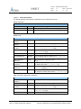
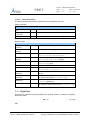
Document Change Record
Issue
Date
Affected Chapter/Section/Page
Reason for Change
Brief Description of Change
Draft
1.1
2012-10-15
2012-10-16
All
7, 10
1.2
2012-10-18
10
1.3
1.4
2012-10-30
2012-11-23
2.1, 7, 8, 9, 10.1.1
All
1.5
2012-12-19
1.2, 3
1.6
2013-07-08
7, 9
Added PEC (position) and
reaction wheel models
1.7
2013-07-26
7
PEC (position) updated
Astos Solutions GmbH
Grund 1, 78089 Unterkirnach, Germany
Draft issue
Added chapters
Added references
PointingSat example
to
the
Customer Review
Customer Review
Added references, added
paragraph
All Rights Reserved - Copyright 2013 per ISO 16016
Copying and distribution is prohibited without express authority.
Doc.No: ASTOS-PEET-SUM-001
PEET
Astos
Solutions
Issue:
1.7
Date: 2013-07-26
Page:
3
of:
60
Table of Contents
1
2
Applicable and Reference Documents ......................................................... 6
1.1
Applicable Documents ....................................................................................... 6
1.2
Reference Documents ....................................................................................... 6
Terms, Definitions and Abbreviated Terms .................................................. 7
2.1
Acronyms ........................................................................................................... 7
2.2
Definitions .......................................................................................................... 7
3
Introduction.................................................................................................. 8
4
Prerequisites ............................................................................................... 9
5
Installing and running PEET ...................................................................... 10
6
7
5.1
Installation ........................................................................................................ 10
5.2
Running PEET ................................................................................................. 10
Graphical User Interface ............................................................................ 11
6.1
The System View ............................................................................................. 11
6.2
The Tree View .................................................................................................. 13
6.3
The Database Browser .................................................................................... 14
Block Types ............................................................................................... 15
7.1
7.1.1
7.2
7.2.1
7.3
7.3.1
7.4
7.4.1
7.5
7.5.1
7.6
Coordinate Transformation Block .................................................................... 15
Block Parameters ..................................................................................... 15
Dynamic System Block .................................................................................... 15
Block Parameters ..................................................................................... 15
Feedback System Block .................................................................................. 17
Block Parameters ..................................................................................... 17
Flexible Plant Block .......................................................................................... 19
Block Parameters ..................................................................................... 19
Gyro Rate Noise Block ..................................................................................... 19
Block Parameters ..................................................................................... 20
Gyro-Stellar Estimator Block ............................................................................ 20
7.6.1
Block Parameters ..................................................................................... 21
7.6.2
Block inputs and outputs .......................................................................... 21
7.7
7.7.1
Mapping Block ................................................................................................. 21
Block Parameters ..................................................................................... 22
Astos Solutions GmbH
Grund 1, 78089 Unterkirnach, Germany
All Rights Reserved - Copyright 2013 per ISO 16016
Copying and distribution is prohibited without express authority.
Doc.No: ASTOS-PEET-SUM-001
PEET
Astos
Solutions
7.8
Issue:
1.7
Date: 2013-07-26
Page:
4
of:
60
PEC Blocks ...................................................................................................... 22
7.8.1
PEC (Pointing) .......................................................................................... 22
7.8.2
PEC (Position) .......................................................................................... 22
7.9
PES Block ........................................................................................................ 24
7.9.1
Time Constant Block Parameters ............................................................. 24
7.9.2
Time Random Block Parameters.............................................................. 27
7.10
Reaction Wheel Model ..................................................................................... 31
7.10.1
Reaction Wheel (Force) ............................................................................ 31
7.10.2
Reaction Wheel (Torque) ......................................................................... 35
7.11
Rigid Plant ........................................................................................................ 37
7.11.1
7.12
PID Controller .................................................................................................. 38
7.12.1
7.13
Block Parameters ..................................................................................... 38
Block Parameters ..................................................................................... 38
Static System Block ......................................................................................... 39
7.13.1
Block Parameters ..................................................................................... 39
7.14
Summation Block ............................................................................................. 39
7.15
Star Tracker Noise Block ................................................................................. 39
7.15.1
8
Block Parameters ..................................................................................... 40
Building Pointing Systems Using PEET ..................................................... 42
8.1
Global settings ................................................................................................. 43
8.2
Configuring blocks ........................................................................................... 43
8.2.1
Linking to external data ............................................................................ 43
8.2.2
Sensitivity analysis.................................................................................... 45
8.3
9
Container blocks .............................................................................................. 46
Computing Pointing Errors Using PEET .................................................... 47
9.1
10
Pointing budget reports .................................................................................... 49
PointingSat Example ................................................................................. 50
10.1
Building the pointing system ............................................................................ 50
10.1.1
Connecting blocks .................................................................................... 54
10.1.2
Defining correlations between error sources ............................................ 56
10.2
Computing pointing errors................................................................................ 56
10.2.1
Creating error indices ............................................................................... 56
10.2.2
Perform error computation ........................................................................ 58
Astos Solutions GmbH
Grund 1, 78089 Unterkirnach, Germany
All Rights Reserved - Copyright 2013 per ISO 16016
Copying and distribution is prohibited without express authority.
Doc.No: ASTOS-PEET-SUM-001
PEET
Astos
Solutions
10.2.3
Issue:
1.7
Date: 2013-07-26
Page:
5
of:
60
Analyse pointing errors ............................................................................. 59
Astos Solutions GmbH
Grund 1, 78089 Unterkirnach, Germany
All Rights Reserved - Copyright 2013 per ISO 16016
Copying and distribution is prohibited without express authority.
Doc.No: ASTOS-PEET-SUM-001
Astos
Solutions
1
PEET
Issue:
1.7
Date: 2013-07-26
Page:
6
of:
60
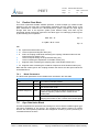
Applicable and Reference Documents
1.1
Applicable Documents
[AD1]
ECSS-E-ST-60-10C; Control Performance Standard ECSS-E-ST-60-10C, ESAESTEC Requirements & Standards Division, 2008.
ESSB-HB-E-003; ESA Pointing Error Engineering Handbook, Issue 1, 19 July
2011
[AD2]
1.2
Reference Documents
[RD1]
[RD2]
ASTOS-PEET-TN-001_Iss1.0; PointingSat Definition
IEEE-STD 952-1997 (R2003); IEEE Standard Specification Format Guide and
Test Procedure for Single-Axis Interferometric Fiber Optic Gyros
[RD3] Ott T., Benoit A., Van den Braembussche P., Fichter W., “ESA Pointing Error
Engineering Handbook”, 8th International ESA Conference on Guidance,
Navigation & Control Systems, Karlovy Vary CZ, June 2011.
[RD4] Ott T., Fichter W., Bennani S., Winkler S.‚ "Precision Pointing H∞-Control Design
for Absolute-, Windowed-, and Stability-Time Errors", manuscript submitted to
CEAS Space Journal.
[RD5] Hirth M., Brandt N., Fichter W., "Inertial Sensing for Future Gravity Missions",
GEOTECHNOLOGIEN Science Report No.17, Observation of the System Earth
from Space, Bonn, 2010, ISSN: 1619-7399.
[RD6] Hirth M., Fichter W., et al., "Optical Metrology Alignment and Impact on the
Measurement Performance of the LISA Technology Package", Journal of Physics
Conference Series, 7th International LISA Symposium, Barcelona, Spain, 2008.
[RD7] NPD/5022/TD/TR/001 v1.r1.m0; "Error Budgets for Formation Flying Missions",
Harwood A. March 2008
[RD8] PFF-MEMO-MC-001; "Reaction Wheel Microvibration Model", Memo, Casasco
M., April 2013.
[RD9] Masterson R.A., "Development and Validation of Empirical and Analytical
Reaction Wheel Disturbance Models", Master Thesis, Massachussetts Institute of
Technology, June 1999.P3-EST-TN-7001;
[RD10] Masterson R.A., Miller D.W., Grogan R.L. "Development of Empirical and
Analytical Reaction Wheel Disturbance Models", AIAA 99-1204, AIAA Structural
Dynamics and Materials Conference, St. Louis, USA, 1999.
Astos Solutions GmbH
Grund 1, 78089 Unterkirnach, Germany
All Rights Reserved - Copyright 2013 per ISO 16016
Copying and distribution is prohibited without express authority.
Doc.No: ASTOS-PEET-SUM-001
PEET
Astos
Solutions
2
2.1
Issue:
1.7
Date: 2013-07-26
Page:
7
of:
60
Terms, Definitions and Abbreviated Terms
Acronyms
The following abbreviations are used throughout this document.
Acronyms
PEET
CDF
GUI
PEC
PES
PSD
CRV
RV
RP
Pointing error engineering tool
ESA/ESTEC Concurrent Design Facility
Graphical user interface
Pointing/Performance error contributor
Pointing error source
Power spectral density
Constant random variable
Random variable
Random process
2.2
Definitions
The following definitions are used throughout this document.
Definitions
Signal
Block mask
The information about the pointing error which will be
exchanged between adjacent blocks.
The input dialog provided by the blocks for parameter input.
Astos Solutions GmbH
Grund 1, 78089 Unterkirnach, Germany
All Rights Reserved - Copyright 2013 per ISO 16016
Copying and distribution is prohibited without express authority.
Doc.No: ASTOS-PEET-SUM-001
Astos
Solutions
3
PEET
Issue:
1.7
Date: 2013-07-26
Page:
8
of:
60
Introduction
The ECSS Control Performance Standard E-ST-60-10C [AD1], published in November
2008, provides solid and exact mathematical elements to build up a performance error
budget. However, an additional document that provides guidelines and summation rules
based on the top level clauses gathered in this ECSS-E-ST-60-10C standard was
considered necessary by ESA to provide ESA projects with a clear pointing error
engineering methodology. This methodology is the basis for a step-by-step process with
guidelines, recommendations and examples consistent with and complementing the
ECSS standard. The answer to this necessity is the ESA Pointing Error Engineering
(PEE) Handbook [AD2] that was published in 2011 as ESA applicable document with the
reference ESSB-HB-E-003.
According to the methodology defined in the Control Performance Standard [AD1] and in
the Pointing Error Engineering Handbook [AD2], a software tool called PEET (Pointing
Error Engineering Tool) was developed to support system engineers and control
engineers working in CDF and in Phase A studies in performing preliminary pointing error
engineering tasks.
PEET was designed as an extension to MATLAB. It uses the computational power
provided by MATLAB and provides the user a graphical user interface suitable for
building pointing systems and analysing pointing errors. The graphical user interface is
implemented in Java. The core of the PEET software, containing the mathematical
algorithms for error computation, is implemented using MATLAB classes. PEET runs
completely inside the MATLAB environment.
The MATLAB classes are based on the iFR Precision Analysis and Control Toolbox in
MATLAB. This toolbox provides algorithms in MATLAB for the research results published
in [RD3] - [RD6], but also to not yet published results. In order to integrate the toolbox in
the PEET framework, it has been extended and adapted by the subcontractor iFR.
This software user manual explains how pointing systems can be build up in PEET and
how pointing error computations can be performed. Chapter 6 will introduce the reader to
the graphical user interface in general and to the various window types, the user is faced
with while building up pointing systems and analysing pointing errors. How to build up
pointing systems is explained in detail in chapter 8 while chapter 9 gives a detailed
explanation about performing and analysing error computations.
Astos Solutions GmbH
Grund 1, 78089 Unterkirnach, Germany
All Rights Reserved - Copyright 2013 per ISO 16016
Copying and distribution is prohibited without express authority.
Doc.No: ASTOS-PEET-SUM-001
Astos
Solutions
4
PEET
Issue:
1.7
Date: 2013-07-26
Page:
9
of:
60
Prerequisites
The following items are mandatory to install PEET.
Standard Desktop PC
Windows XP or higher
MATLAB 2011b or higher
MATLAB Control System Toolbox
Astos Solutions GmbH
Grund 1, 78089 Unterkirnach, Germany
All Rights Reserved - Copyright 2013 per ISO 16016
Copying and distribution is prohibited without express authority.
Doc.No: ASTOS-PEET-SUM-001
PEET
Astos
Solutions
5
Issue:
1.7
Date: 2013-07-26
Page:
10
of:
60
Installing and running PEET
5.1
Installation
PEET can be installed to any location by simply placing the PEET folder at the desired
location. The PEET folder must be writeable for all users. PEET is completely running
inside the MATLAB environment. As already mentioned in the introduction, the graphical
user interface is written in Java. All the java classes required by PEET are stored in the
following jar files.
peet.jar, graphical user interface of PEET
jxl.jar, Java classes used for import and export of Excel data.
piccolo2d-core-1.3.1.jar, graphical framework used by the GUI.
piccolo2d-extras-1.3.1.jar, graphical framework used by the GUI.
In order that MATLAB can find the Java classes, the absolute paths to all the jar files
must be added to the static class path of MATLAB. This is done by adding the absolute
paths to the classpath.txt file located in the toolbox\local folder of your MATLAB
installation. If this file cannot be edited or should be kept in its original state, it is also
possible to create a local classpath.txt file for each user. Simply copy the content of the
original classpath.txt file to a new classpath.txt file located in the Documents/MATLAB
folder (or My Documents/MATLAB on Windows platforms other than Windows Vista).
This local classpath.txt file will be used at start-up. The required jar files can now be
added to the new classpath.txt file.
5.2
Running PEET
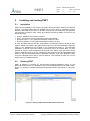
PEET is started by entering int_.esa.peet.gui.Peet.main({'installation_path'}) on the
MATLAB command line. For installation_path, use the absolute path to the PEET folder.
Figure 5-1 shows an example assuming that the PEET folder was placed in c:\Program
Files.
Figure 5-1: Running PEET from the MATLAB command line
Astos Solutions GmbH
Grund 1, 78089 Unterkirnach, Germany
All Rights Reserved - Copyright 2013 per ISO 16016
Copying and distribution is prohibited without express authority.
Doc.No: ASTOS-PEET-SUM-001
PEET
Astos
Solutions
6
Issue:
1.7
Date: 2013-07-26
Page:
11
of:
60
Graphical User Interface
This chapter will provide the user an introduction to the graphical user interface and to the
various window types he will face while building up pointing systems and analysing
pointing errors.
6.1
The System View
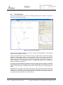
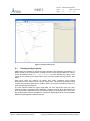
The system view is the main window of PEET. It will be the first window after PEET has
been started. It is mainly used to build up the pointing system in a way similar to Simulink.
A detailed description on how a pointing system can be build is given in chapter 8.
Figure 6-1: The System View window
Figure 6-1 shows the system view window. This window contains a menu bar, a tool bar
and the system view, covering most of the window.
The file menu contains all actions related to file handling e.g. opening an existing pointing
system, creating an empty pointing system or saving the current pointing system. It also
contains the menu entry used to create the reports for the currently loaded pointing
system.
The setup menu contains all menu entries used for configuring the current pointing
system. Using the setup menu, the user can define the correlations between the pointing
error sources, define the error indices he is interested in and define the global parameters
applicable for the pointing system.
Astos Solutions GmbH
Grund 1, 78089 Unterkirnach, Germany
All Rights Reserved - Copyright 2013 per ISO 16016
Copying and distribution is prohibited without express authority.
Doc.No: ASTOS-PEET-SUM-001
Astos
Solutions
PEET
Issue:
1.7
Date: 2013-07-26
Page:
12
of:
60
The Database menu contains all actions related to the block database. It provides the
user the possibility to open the database browser and to manage user defined block
types.
Finally the Windows menu gives the user access to all window types and to actions
related to the system view e.g. fit the current system view in order to show the whole
pointing system.
The tool bar contains some short cuts to menu entries. Starting on the left, the user can
open the database browser, open the tree view, delete the selected element or fit the
system view to show the whole pointing system.
The main part of the system view window shows the currently loaded pointing system.
Each pointing system consists of a number of blocks and connection between the blocks.
The location of the blocks can be changed by selecting a block and dragging it to the
desired location. It is also possible to zoom the system view by pressing the right mouse
button and moving the mouse to the left (zoom out) or right (zoom in).
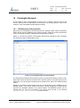
For editing a connection between blocks, the user has some possibilities. Figure 6-2
shows a selected connection which now can be edited by the user.
Figure 6-2: Editing connections
To edit the location of the connection, the user has to click on one of the red spots of the
line. Afterwards the spot can be moved to the desired location. In this way, connections
are completely adjustable by the user.
Astos Solutions GmbH
Grund 1, 78089 Unterkirnach, Germany
All Rights Reserved - Copyright 2013 per ISO 16016
Copying and distribution is prohibited without express authority.
Doc.No: ASTOS-PEET-SUM-001
PEET
Astos
Solutions
6.2
Issue:
1.7
Date: 2013-07-26
Page:
13
of:
60
The Tree View
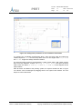
The tree view window can be used to analyse pointing errors. Figure 6-3 gives an
example of the tree view window.
Figure 6-3: The Tree View window
The tree view window consists of a tool bar, a tree-like representation of the pointing
system and an information section.
Using the drop down menu in the tool bar, the user can select the error index he wants to
analyse. The information shown in the information section on the right of the window
shows the current signal data for the selected error index and the selected block. To
select a block, the user simply clicks on the block of interest. If no block is selected, no
data is available in the information section. A detailed description of the information
section is provided in chapter 9.
The user can switch between the data of input and output ports of a block by selecting
the associated tab in the information panel. There will be always on output port tab. The
number of input port tabs is related to the number of input ports of the currently selected
block.
Compared to the system view window, the blocks and connections cannot be moved
inside the tree view window. The tree view window automatically organizes all blocks and
connections in a tree-like structure starting with the error sources on the upper most level
and ending with the PEC block on the lowest level.
Astos Solutions GmbH
Grund 1, 78089 Unterkirnach, Germany
All Rights Reserved - Copyright 2013 per ISO 16016
Copying and distribution is prohibited without express authority.
Doc.No: ASTOS-PEET-SUM-001
Astos
Solutions
6.3
PEET
Issue:
1.7
Date: 2013-07-26
Page:
14
of:
60
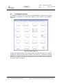
The Database Browser
The database browser provides access to the block database. It organizes all available
block types in categories. For each block category, a tab is shown in the database
browser.
Figure 6-4: Database Browser
The first tab contains all block types used by PEET. All other tabs represent a category
containing a subset of the block types available on the first tab. To add blocks from the
database to the pointing system, the desired block must be dragged from the database
browser to the system view window. A detailed description on how a pointing system will
be created is given in chapter 8.
Astos Solutions GmbH
Grund 1, 78089 Unterkirnach, Germany
All Rights Reserved - Copyright 2013 per ISO 16016
Copying and distribution is prohibited without express authority.
Doc.No: ASTOS-PEET-SUM-001
PEET
Astos
Solutions
7
Issue:
1.7
Date: 2013-07-26
Page:
15
of:
60
Block Types
This chapter explains the various block types and their required parameters. For each
block type, the meaning of the block parameters will be explained in detail.
If not otherwise stated in the software user manual or in the block masks, all parameters
must be provided in SI units (e.g. angles must be defined in radian). It is up to the user to
ensure that the numbers are consistent across the pointing system. If a block mask
forces the user to provide parameters in Non-SI units, these parameters will be converted
to SI units internally.
7.1
Coordinate Transformation Block
The coordinate transformation block is used to transform signal data from one coordinate
system to another coordinate system. The coordinate system transformation is defined by
an Euler transformation using three angles and a rotation sequence. The resulting matrix
is used as static system gain to transfer the input signal.
7.1.1
Block Parameters
The coordinate transformation parameters offered by the block mask are listed in the
following table.
Block mask parameters
Rotation sequence
Selection The rotation sequence used for the Euler transformation.
Possible values are 1-2-3, 1-3-2, 2-1-3, 2-3-1,
3-1-2, 3-2-1, 1-2-1, 1-3-1, 2-1-2, 2-3-2,
3-1-3 and 3-2-3.
Phi
Double
Theta
Double
Psi
Double
7.2
The angle describing the rotation around the first axis of
the rotation sequence.
The angle describing the rotation around the second axis
of the rotation sequence.
The angle describing the rotation around the third axis of
the rotation sequence.
Dynamic System Block
The dynamic system block is used to model any kind of dynamic systems. In general, the
system transfer is described by a 3x3 matrix. The elements of the system transfer matrix
can be transfer functions, frequency-response models or zero-pole-gain models.
Alternatively a state space model can be provided which defines the dynamic system.
Internally all inputs are transformed to a state space model which will be used for the
system transfer.
7.2.1
Block Parameters
Depending on the matrix element type, different parameters are provided by the block
mask as described in the next subchapters. The two parameters which are always
available independent of the matrix element type are listed in the next table.
Astos Solutions GmbH
Grund 1, 78089 Unterkirnach, Germany
All Rights Reserved - Copyright 2013 per ISO 16016
Copying and distribution is prohibited without express authority.
Doc.No: ASTOS-PEET-SUM-001
PEET
Astos
Solutions
Issue:
1.7
Date: 2013-07-26
Page:
16
of:
Representation
Block mask parameters
Selection The type of the matrix elements. Possible values are
Transfer function, Frequency-Response,
Zero-Pole-Gain and State space.
Matrix element
Selection
60
A drop down menu providing the user the possibility to
choose the element of the system transfer matrix for
editing. This parameter is only used by the block mask
and has no effect on the error calculations. In general,
always the whole 3x3 transfer matrix will be used for the
system transfer. Possible values are x-x, x-y, x-z,
y-x, y-y, y-z, z-x, z-y and z-z. Only
available if the representation is not set to State
space. In this case the state-space model defines the
entire 3x3 system.
7.2.1.1
Transfer Function Parameters
A transfer function is described by the coefficients for its numerator and its denominator.
The parameters provided by the block mask are listed below.
Numerator
List
Denominator
List
Block mask parameters
A list of coefficients defining the numerator of the transfer
function. Each coefficient is of type double.
A list of coefficients defining the denominator of the
transfer function. Each coefficient is of type double.
7.2.1.2
Zero-Pole-Gain Parameters
The zero-pole-gain model is described by a list of coefficients describing the zeros of the
transfer function, a list of coefficients describing the poles of the transfer function and a
gain value. The block mask provides the following parameters.
Block mask parameters
Zeros
Poles
Gain
List
A list of coefficients defining the zeros of the transfer
function. Each coefficient is of type double.
List
A list of coefficients defining the poles of the transfer
function. Each coefficient is of type double.
Double A single double value describing the gain of the transfer
function.
7.2.1.3
State Space Parameters
The state space model is described by the number of state variables (n) and by four
matrices A, B, C and D.
Block mask parameters
State variables Selection
A
nxn Matrix
Astos Solutions GmbH
Grund 1, 78089 Unterkirnach, Germany
The number of state variables. Possible values are in the
range from 1 to 99.
The state matrix of the state space model. Each matrix
element is a scalar value of type double.
All Rights Reserved - Copyright 2013 per ISO 16016
Copying and distribution is prohibited without express authority.
Doc.No: ASTOS-PEET-SUM-001
PEET
Astos
Solutions
B
Nx3 Matrix
C
3xn Matrix
D
3x3 Matrix
7.3
Issue:
1.7
Date: 2013-07-26
Page:
17
of:
60
The input matrix of the state space model. Each matrix
element is a scalar value of type double.
The output matrix of the state space model. Each matrix
element is a scalar value of type double.
The feedthrough matrix of the state space model. Each
matrix element is a scalar value of type double.
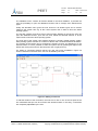
Feedback System Block
Feedback systems are the only block type which allows the user to integrate loops into
the pointing system. The fixed structure of the feedback system implemented by this
block type is shown in Figure 7-1.
Figure 7-1: Feedback system structure
Each of the blocks labelled 1 to 6 can either be turned on or off. If turned on, the user has
to specify the block type and the block parameters. The available block types are a
subset of the blocks available in the database and are explained in chapter 7.3.1. By
turning internal blocks on and off, the user can build up any kind of feedback system
structure required for the pointing error calculations of PEET.
The nodes labelled A to G serves as input or output ports. It is possible to define more
than one input port. The number of output ports is restricted to one. In addition to this
restriction, it is not possible to use one of the nodes as input and output port.
All block parameters are converted internally to state space models. Using this state
space models, an equivalent dynamic system is build up which will be used for the
system transfer.
7.3.1
Block Parameters
The parameters for the feedback system can be divided into two groups. The first set of
parameters deals with the definition of the input and output ports. These parameters are
listed in the next table.
Block mask parameters
Input ports
Selection
Astos Solutions GmbH
Grund 1, 78089 Unterkirnach, Germany
The user can choose one or more input ports. Possible
values are A, B, C, D, E, F and G. The node which is
currently set as output port cannot be selected as input
port.
All Rights Reserved - Copyright 2013 per ISO 16016
Copying and distribution is prohibited without express authority.
Doc.No: ASTOS-PEET-SUM-001
PEET
Astos
Solutions
Output port
Selection
Issue:
1.7
Date: 2013-07-26
Page:
18
of:
60
The user can select the output port. Only one node can be
set as output port. Possible values are A, B, C, D, E,
F and G. If the user selects a node which is currently used
as input port, this port is removed from the list of input
ports and set as the one and only output port.
The second set of parameters deals with the parameter settings for the blocks. Each of
the blocks provides the same parameters which are listed below. In general any system
transfer block from the database can be selected with the only restriction of one single 3D
input and one single 3D output.
Block mask parameters
Block type
Selection
The type of the block. Possible values are Unused,
Coordinate Transformation, Dynamic System,
Flexible Plant, Rigid Plant, Static System
and PID Controller.
Using the block type Unused turns off the block. By turning off a block, the signal can
pass this block without any modifications to it. If a block type different than Unused is
selected, additional parameters are available. These parameters are described in the
next chapters.
7.3.1.1
Internal Block Type: Coordinate Transformation
The parameters for the coordinate transformation type are the same as for the
Coordinate Transformation block. These parameters are explained in detail in chapter
7.1.
7.3.1.2
Internal Block Type: Dynamic System
The parameters for the dynamic system type are the same as for the Dynamic System
block. These parameters are explained in detail in chapter 7.2.
7.3.1.3
Internal Block Type: Flexible Plant
The parameters for the flexible plant type are the same as for the Flexible Plant block.
These parameters are explained in detail in chapter 7.4.
7.3.1.4
Internal Block Type: Rigid Plant
The parameters for the rigid plant type are the same as for the Rigid Plant block. These
parameters are explained in detail in chapter 7.11.
7.3.1.5
Internal Block Type: Static System
The parameters for the static system type are the same as for the Static System block.
These parameters are explained in detail in chapter 7.13.
7.3.1.6
Internal Block Type: PID Controller
The parameters for the PID controller system type are the same as for the PID Controller
block. These parameters are explained in detail in chapter 7.12.
Astos Solutions GmbH
Grund 1, 78089 Unterkirnach, Germany
All Rights Reserved - Copyright 2013 per ISO 16016
Copying and distribution is prohibited without express authority.
Doc.No: ASTOS-PEET-SUM-001
PEET
Astos
Solutions
7.4
Issue:
1.7
Date: 2013-07-26
Page:
19
of:
60
Flexible Plant Block
This block implements flexible satellite dynamics. It takes multiple (n) flexible modes
defined by the user with their corresponding parameters and the inertia tensor of the
plant. Afterwards it constructs an n-termed dynamic system, transfers the input signal
through each term of the dynamic system (each flexible mode), and sums up the
transferred signals as the final response of this block type. The underlying model is given
by the following set of equations:
δα
N
Θω
Eq 7-1
2 ζ Ω α Ω2 α δ T Ω
α
Eq 7-2
with:
Θ
ω
δ
N
α
spacecraft inertia matrix (3x3)
vector of spacecraft angular rates (3x1)
matrix of coupling coefficients describing the coupling of flexible modes into the
spacecraft body rotation (3xn)
vector of torques acting on the spacecraft body (3x1)
vector containing the amplitudes of n flexible modes (nx1)
ζ
Ω
diagonal matrix containing the damping ratio of the flexible modes (nxn)
diagonal matrix containing the cantilever frequencies of the flexible modes (nxn)
Note that this model ignores the coupling between the flexure and the spacecraft linear
acceleration/force
7.4.1
Block Parameters
The block mask parameters for the flexible block are listed in the next table.
Block mask parameters
Mode
Integer
Inertia
Matrix
Coupling coefficients Matrix
Cantilever frequency Matrix
Damping ratio
7.5
Matrix
The number of flexible modes.
A 3x3 matrix containing the inertia tensor.
A 3xn matrix containing the coupling coefficients for each
axis and for each mode.
An nx1 vector containing the diagonal elements of the
cantilever frequency matrix for the n modes of the
flexible plant.
An nx1 vector containing the diagonal elements of
damping ratio matrix for the n modes of the flexible plant.
Gyro Rate Noise Block
This block implements a special kind of pointing error source which combines typical gyro
rate noise contributors in one source. The resulting noise shape is fitted to a transfer
function with user-specified parameters and mapped to all axes (x,y and z) assuming no
correlation between the axes.
Astos Solutions GmbH
Grund 1, 78089 Unterkirnach, Germany
All Rights Reserved - Copyright 2013 per ISO 16016
Copying and distribution is prohibited without express authority.
Doc.No: ASTOS-PEET-SUM-001
PEET
Astos
Solutions
7.5.1
Issue:
1.7
Date: 2013-07-26
Page:
20
of:
60
Block Parameters
The GUI parameters for the gyro rate noise block are shown in the table below.
Block mask parameters
Min. pole order
Max. pole order
Number of frequency
points
Angle random walk (N)
Rate random walk (K)
Bias instability (B)
Quantization noise (Q)
Time window (T)
Double
Double
Double
Minimum pole order for rational fit of PSD
Maximum pole order for rational fit of PSD
Frequency point used for rational fitting
Double
Double
Double
Double
Double
The magnitude of the angle random walk [°/√h].
3/2
The magnitude of the angle random walk [°/h ].
The magnitude of the bias instability [°/h].
The magnitude of the quantization noise [arcsec].
The time window [s].
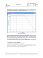
Using the parameters defined, the Gyro Rate Noise block realizes a PSD type error
source with a spectral behaviour as shown in Figure 7-2. For further information about the
involved parameters see appendix B of [RD2].
Figure 7-2: Gyro noise PSD derived from typical specifications [RD2] .
7.6
Gyro-Stellar Estimator Block
This block implements the gyro-stellar estimator in PEET. It is the only block type which
has more than one output port. The parameters required by this block type are the two
Kalman gains Kp and Kd. In general, the Kalman estimator is realized as a dynamic
system, which takes 3 inputs and 2 outputs. It computes the signal transfer according to
the fixed Kalman estimator structure using user input gains from the model given below
individually for each axis:
Astos Solutions GmbH
Grund 1, 78089 Unterkirnach, Germany
All Rights Reserved - Copyright 2013 per ISO 16016
Copying and distribution is prohibited without express authority.
Doc.No: ASTOS-PEET-SUM-001
PEET
Astos
Solutions
~
φ
1
~ 2
B
s K ps K 2
7.6.1
Issue:
1.7
Date: 2013-07-26
Page:
21
of:
(K p s K d ) n Str s n gyro Bgyro
K s n K n (s K ) B
d gyro
p
gyro
d Str
60
Eq 7-3
Block Parameters
The GUI parameters for the gyro-stellar estimator block are listed in the next table.
Kalman gain Kp Vector
Kalman gain Kd Vector
7.6.2
Block mask parameters
A three dimensional vector containing the Kalman gains
Kp for the x,y and z axis. The elements of the vector are of
type double.
A three dimensional vector containing the Kalman gains
Kd for the x,y and z axis. The elements of the vector are of
type double.
Block inputs and outputs
The gyro-stellar estimator block offers the user three input and two output ports. All of
these ports are optional and can be left unconnected. An explanation of these ports is
provided by the tables below.
n_str
n_gyro
b_gyro
Input ports
The star-tracker measurement noise.
The gyro rate measurement noise.
The gyro drift bias noise ('Rate random walk').
Output ports
φ_est
B_est
The attitude estimation error.
The gyro bias estimation error
Note the gyro noise contributions can be realized in different ways: Either as individual
signals using both n_gyro and b_gyro or by combining the gyro drift bias and rate noise to
a total noise using the Gyro Rate Noise block presented in section 7.5 only and feeding it
to the n_gyro input only (see also definition of PES 7 in the PointingSat example for
further details).
7.7
Mapping Block
The Mapping block is used to map a 1D signal to a spatially distributed 3D signal, i.e.
mapping thruster noise from the axis of each thruster to the reference frame of the
pointing error. The user input consists of the number of devices (n) that are mapped by
this block and the nx3 mapping matrix. The mapping block extends the 1D signal to an
nxn signal, and transfers the nxn signal through the nx3 mapping matrix, which serves as
a static system. Finally it produces a three dimensional signal.
Astos Solutions GmbH
Grund 1, 78089 Unterkirnach, Germany
All Rights Reserved - Copyright 2013 per ISO 16016
Copying and distribution is prohibited without express authority.
Doc.No: ASTOS-PEET-SUM-001
PEET
Astos
Solutions
7.7.1
Issue:
1.7
Date: 2013-07-26
Page:
22
of:
60
Block Parameters
The next table explains the block mask parameters for the Mapping block.
Block mask parameters
Number of devices
Selection
Mapping matrix
Matrix
7.8
The number of devices which will be mapped by this
block. Possible values are in the range from 1 to 99.
The nx3 mapping matrix with as many rows as devices
are defined. The columns contain the mappings for the
x, y and z axis.
PEC Blocks
The pointing error contributor block represents the "endpoint" of each PEET system
model at which the resulting total error contribution shall be evaluated. The evaluation is
realized according to AST-4 of [AD2] and the results are grouped into time-constant,
time-random and total error contribution. The usage of a PEC block is mandatory for each
PEET system and only one PEC block can be used in a system. Two kinds of blocks are
available in the block database:
7.8.1
PEC (Pointing)
The PEC (Pointing) block is the standard block for the overall error evaluation. It has no
parameters and only one single input which corresponds to the total error signal of the
system under consideration. The content of the different parts of the input signal (CRV,
RV, drift, periodic signal and random process part) is summed according to AST-4 of
[AD2] after the equivalent variance of a potential random process signal is computed
within the user-defined global evaluation bandwidth.
The overall error is computed per axis (x,y,z) and with respect to the user defined LOS
axis. Note that the latter is the only special feature that links the block really to pointing.
Disregarding the LOS error, this block (and PEET) could be used to compute any kind of
3-axis budget (i.e. PEET could generally be understood as "Performance Error
Engineering Tool" rather than a "Pointing Error Engineering Tool" only.
7.8.2
PEC (Position)
The PEC (Position) realizes a special case for the overall error evaluation. It allows the
computation of a position/displacement error budget which is the result of "pure" 3-axis
position errors and 3-axis attitude errors which couple into equivalent position errors due
to dedicated "lever arms" (e.g. as it is the case for formation flying missions such as
PROBA 3). The implemented model is based on Eq.5 in [RD7]:
N att
μ tot,x μ pos ,x y i μ att,z ,i z i μ att, y,i
i 1
N att
N att
2
2 2
σ 2tot,x σ 2pos ,x y i2 σ att
,z.i z i σ att, y ,i
i 1
N att
2
2 2
μ tot, y μ pos , y z i μ att,z,i x i μ att,z ,i σ 2tot, y σ 2pos , y z i2 σ att
, x .i x i σ att,z ,i
i 1
N att
i 1
N att
i 1
i 1
2
2 2
μ tot,z μ pos ,z x i μ att,z ,i y i μ att,x ,i σ 2tot,z σ 2pos ,z x i2 σ att
, y.i y i σ att, x ,i
Eq 7-4
with (axis index omitted):
Astos Solutions GmbH
Grund 1, 78089 Unterkirnach, Germany
All Rights Reserved - Copyright 2013 per ISO 16016
Copying and distribution is prohibited without express authority.
Doc.No: ASTOS-PEET-SUM-001
PEET
Astos
Solutions
Issue:
1.7
Date: 2013-07-26
Page:
23
of:
μ tot
total mean of resulting displacement error
σ tot
total standard deviation of resulting displacement error
μ pos
overall mean of "pure" position error contributors
σ pos
overall standard deviation of "pure" position error contributors
N att
number of attitude error coupling to position
μ att,i
mean of i-th attitude error
σ att,i
standard deviation of i-th attitude error
x i , yi , zi
components of coupling vector of i-th attitude error
60
Different to Eq. 5 in [RD7] there is no summation over different position error contributors.
The summation of these contributors has to be realized using standard Sum blocks in the
PEET system (this allows the usage of one single position error input for the PEC
(Position) block).
Above realization corresponds to the option Exact in the block's Summation rule dropdown menu. In case the directions ('sign relations') of individual contributors are not
exactly known a priori, PEET alternatively offers of a more conservative approach using
the Worst case option. Here, the total mean is computed using absolute values
according to the following equation:
μ tot, x μ pos, x
μ tot, y μ pos , y
μ tot, z μ pos, z
yi μ att, z,i zi μ att, y,i
N att
i 1
zi μ att, z,i x i μ att, z,i
N att
i 1
Eq 7-5
x i μ att, z,i yi μ att, x ,i
N att
i 1
The number of additional block inputs for attitude errors depends on the settings of the
parameters which are listed in the table below:
Summation rule
Block mask parameters
Selection Desired summation for the means in the equation
above (see Eq. 5 in [RD7]), possible selections are
Worst case and Exact.
Number of attitude
contributors
Selection
Attitude coupling
vector
Matrix
The number of attitude contributors (Natt) that couple
with different lever arms to position errors (determines
the number of additional block input ports).
Nattx3 mapping matrix with as many rows as attitude
contributors are defined. The columns contain the x, y
and z components of the i-th coupling vector.
The tree-view of the block finally provides the following information:
signal content of each attitude and position error signals
Astos Solutions GmbH
Grund 1, 78089 Unterkirnach, Germany
All Rights Reserved - Copyright 2013 per ISO 16016
Copying and distribution is prohibited without express authority.
Doc.No: ASTOS-PEET-SUM-001
PEET
Astos
Solutions
Issue:
1.7
Date: 2013-07-26
Page:
24
of:
60
the total mean and standard deviation of the resulting displacement error (timeconstant, time-random and overall contribution)
the mean and standard deviation of the "pure" position error contributor only (timeconstant, time-random and overall contribution)
the mean and standard deviation of the position error due to all the attitude
contributors only (time-constant, time-random and overall contribution)
7.9
PES Block
The pointing error source block is used to model all kind of error sources applicable to
pointing error calculations. Each pointing error source consists of a time constant part
and a time random part. The time constant part is defined by a probability distribution
function. The time random part is either defined as a random variable or as a random
process. Internally, the time constant part and the time random part of type random
variable are converted to an equivalent Gaussian distribution. If the time random part is
described as a random process, it is converted to a state space representation. The
signal generated by a pointing error source block can either be one dimensional or three
dimensional. The dimension of the signal is set by the parameter listed in the table below.
The dimension applies to the time constant part as well as to the time random part.
Block mask parameters
The dimension of the output signal of the PES block.
Possible values are 1D and 3D.
Signal dimension
Selection
Use time constant
part
Use time random
part
Checkbox A flag indicating if the pointing error source provides a
time constant part or not.
Checkbox A flag indicating if the pointing error source provides a
time random part or not.
7.9.1
Time Constant Block Parameters
The time constant part of the pointing error source block is defined by using a probability
distribution function. The parameter responsible for the type of the probability distribution
function is given in the next table.
Distribution type
Block mask parameters
Selection The probability distribution function used to specify the
time constant part of the pointing error source block.
Possible values are Discrete, Uniform, Bimodal,
Gaussian and Rayleigh.
Depending on the distribution, additional block mask parameters are available to the
user. The next subchapters will list the parameters for each probability distribution
function applicable for the time constant part.
7.9.1.1
Discrete Distribution Parameters
A discrete distribution is a probability distribution whose variables can only take discrete
values. In the context of PEET, only the mean value must be given by the user. The
parameters provided by the block mask are shown in the next table.
Astos Solutions GmbH
Grund 1, 78089 Unterkirnach, Germany
All Rights Reserved - Copyright 2013 per ISO 16016
Copying and distribution is prohibited without express authority.
Doc.No: ASTOS-PEET-SUM-001
PEET
Astos
Solutions
Mean value
Issue:
1.7
Date: 2013-07-26
Page:
25
of:
60
Block mask parameters
Double / Vector The mean value of the discrete distribution. In case of a
three dimensional PES, this is a vector containing the
mean values for the x, y and z axis. For a one
dimensional PES, the mean value is a single double
value.
7.9.1.2
Uniform Distribution Parameters
The uniform distribution is a continuous probability distribution with the probability density
function
1
pdf ( x ) b a
0
axb
x a or x b
in which a is called the minimum value and b is called the maximum value. The
parameters for the Uniform probability distribution are listed below.
Minimum
Maximum
Axes correlation
Block mask parameters
Double /
The minimum value of the uniform distribution. In
Vector
case of a three dimensional PES, this is a vector
containing the minimum values for the x, y and z
axis. For a one dimensional PES, the minimum
value is a single double value.
Double /
The maximum value of the uniform distribution. In
Vector
case of a three dimensional PES, this is a vector
containing the maximum values for the x, y and z
axis. For a one dimensional PES, the maximum
value is a single double value.
String
The correlation between the axes. Possible values
are Uncorrelated and Full correlated. Only
available in case of a three dimensional PES.
7.9.1.3
Bimodal Distribution Parameters
The bimodal distribution is a continuous probability distribution with two modes. The
modes appear as two distinct peaks (local maxima) in the probability density function. In
the context of PEET it is sufficient to only specify the amplitude of the local maxima. All
parameters required by the block mask are shown in the next table.
Amplitude
Axes
correlation
Block mask parameters
Double / Vector The amplitude of the bimodal distribution. In case of a
three dimensional PES, this is a vector containing the
amplitudes for the x, y and z axis. For a one dimensional
PES, the amplitude is a single double value.
String
The correlation between the axes. Possible values are
Uncorrelated and Full correlated. Only available
in case of a three dimensional PES.
Astos Solutions GmbH
Grund 1, 78089 Unterkirnach, Germany
All Rights Reserved - Copyright 2013 per ISO 16016
Copying and distribution is prohibited without express authority.
Doc.No: ASTOS-PEET-SUM-001
PEET
Astos
Solutions
Issue:
1.7
Date: 2013-07-26
Page:
26
of:
60
7.9.1.4
Gaussian Distribution Parameters
The Gaussian distribution is a continuous probability distribution with the probability
density function
pdf ( x )
1
σ 2π
e
1 x μ
2 σ
2
2
in which µ is called mean value, σ is called standard deviation and σ is called variance.
The block mask parameters offered by the PES block are listed below.
Block mask parameters
Mean value
Double / Vector
Standard
deviation
Double / Vector
Axes correlation
String
The mean value for the Gaussian distribution. In
case of a three dimensional PES, this is a vector
containing the mean values for the x, y and z axis.
For a one dimensional PES, the mean value is a
single double value.
The standard deviation for the Gaussian
distribution. In case of a three dimensional PES,
this is a vector containing the standard deviation
for the x, y and z axis. For a one dimensional PES,
the standard deviation is a single double value.
The correlation between the axes. Possible values
are Uncorrelated and Full correlated.
Only available in case of a three dimensional PES.
In case of a three dimensional PES, a 3x3 covariance matrix is always used in addition to
the mean value. To simplify the user input, the user can specify the correlation between
the axes. For an uncorrelated or a fully correlated PES, it is required to only define the
standard deviations for the x, y and z axis. These standard deviations are used to
compute the diagonal elements of the covariance matrix. Internally all other elements of
the covariance matrix are set automatically to 0 for an uncorrelated PES and 1 for a fully
correlated PES.
7.9.1.5
Rayleigh Distribution Parameter
The Rayleigh distribution is a continuous probability distribution with the probability
density function
x2
x 2
pdf ( x ) 2 e 2σ
σ
, x 0, σ 0
in which σ is called the Rayleigh parameter. The parameters provided by the block mask
are listed in the next table.
Rayleigh parameter
Block mask parameters
Double / Vector The Rayleigh parameter of the Rayleigh
distribution. In case of a three dimensional PES,
this is a vector containing the Rayleigh
Astos Solutions GmbH
Grund 1, 78089 Unterkirnach, Germany
All Rights Reserved - Copyright 2013 per ISO 16016
Copying and distribution is prohibited without express authority.
Doc.No: ASTOS-PEET-SUM-001
PEET
Astos
Solutions
Axes correlation
7.9.2
String
Issue:
1.7
Date: 2013-07-26
Page:
27
of:
60
parameter for the x, y and z axis. For a one
dimensional PES, the parameter is a single
double value.
The correlation between the axes. Possible
values are Uncorrelated and Full
correlated. Only available in case of a three
dimensional PES.
Time Random Block Parameters
The time random part of the pointing error source can either be defined as a random
variable or as a random process.
If the time random part is defined as a random variable, the user has to choose from a list
of probability distributions. Possible values are Uniform, Gaussian and Drift. For
the Uniform distribution, the parameters are the same as for the time constant part. The
remaining parameters for random variable options are described in chapters 7.9.2.1 and
7.9.2.2
Note that whenever a non-zero mean of a Gaussian RV is defined, PEET automatically
maps this mean to a CRV with discrete distribution and removes it from the RV as it
essentially represents a time-constant part. The same is true for a uniform RV (e.g. in
case of a lower bound 0 and upper bound 3, a CRV with a mean of 1.5 is automatically
created).
If the time random part is defined as a random process, the user has to set the type of the
random process. Possible types are Time series, PSD, Covariance and
Periodic. The parameters for these types are explained in the chapters 7.9.2.3 to
7.9.2.6
7.9.2.1
Random Variable: Gaussian Distribution Parameters
The parameters for the Gaussian distribution of the time random part are listed in the
table below.
Block mask parameters
Mean value
Double /
In case of a three dimensional PES, this is a
Vector
vector containing the mean values for the x, y and
z axis. For a one dimensional PES, the parameter
is a single double value.
Distribution of standard Selection
The ensemble distribution of the standard
deviation
deviation. Possible values are Discrete and
Uniform.
Standard deviation
Double /
Matrix
A 3x1 vector defining the standard deviation for all
axes. In case of a one dimensional error source
the standard deviation is a scalar value. Only
available if the distribution of the standard
deviation is set to Discrete.
Minimum
Double /
Matrix
A 3x1 vector defining the minimum standard
deviation for all axes. In case of a one dimensional
error source the minimum standard deviation is a
scalar value. Only available if the distribution of
Astos Solutions GmbH
Grund 1, 78089 Unterkirnach, Germany
All Rights Reserved - Copyright 2013 per ISO 16016
Copying and distribution is prohibited without express authority.
Doc.No: ASTOS-PEET-SUM-001
PEET
Astos
Solutions
Issue:
1.7
Date: 2013-07-26
Page:
28
of:
60
the standard deviation is set to Uniform.
Maximum
Double /
Matrix
A 3x1 vector defining the maximum standard
deviation for all axes. In case of a one dimensional
error source the maximum standard deviation is a
scalar value. Only available if the distribution of
the standard deviation is set to Uniform.
Axes correlation
String
The correlation between the axes. Possible values
are Uncorrelated and Full correlated.
Only available in case of a three dimensional PES.
7.9.2.2
Random Variable: Drift Distribution Parameters
The drift distribution is only available for the time random part. The parameters provided
by the block mask are listed in the table below.
Block mask parameters
Reset time
Rate distribution
Double
Selection
The time after which the drift will be reset.
A probability distribution used for the drift rate.
Possible values are Discrete, Uniform,
Gaussian and Bimodal.
Axes correlation
String
The correlation between the axes. Possible
values are Uncorrelated and Full
correlated. Only available in case of a three
dimensional PES.
Depending on the rate distribution, additional parameters are available in the block mask.
These additional parameters are explained below.
Discrete Rate Distribution
The parameters for the discrete rate distribution are shown in the next table.
Rate
Block mask parameters
Double / Vector The drift rate. In case of a three dimensional
PES, this is a vector containing the drift rates for
the x, y and z axis. For a one dimensional PES,
the parameter is a single double value.
Uniform Rate Distribution
The table below list all parameters available for the uniform rate distribution.
Block mask parameters
Minimum rate
Maximum rate
Double / Vector The minimum drift rate. In case of a three
dimensional PES, this is a vector containing the
minimum drift rates for the x, y and z axis. For a
one dimensional PES, the parameter is a single
double value.
Double / Vector The maximum drift rate. In case of a three
Astos Solutions GmbH
Grund 1, 78089 Unterkirnach, Germany
All Rights Reserved - Copyright 2013 per ISO 16016
Copying and distribution is prohibited without express authority.
Doc.No: ASTOS-PEET-SUM-001
PEET
Astos
Solutions
Issue:
1.7
Date: 2013-07-26
Page:
29
of:
60
dimensional PES, this is a vector containing the
maximum drift rates for the x, y and z axis. For a
one dimensional PES, the parameter is a single
double value.
Gaussian Rate Distribution
The parameters provided by the block mask for the Gaussian rate distribution are listed
below.
Block mask parameters
Mean rate
Standard deviation
Double / Vector The mean drift rate. In case of a three
dimensional PES, this is a vector containing the
mean drift rates for the x, y and z axis. For a one
dimensional PES, the parameter is a single
double value.
Double / Matrix The standard deviation of the drift rate. In case
of a three dimensional PES, 3x1 vector
containing the standard deviations and the
standard deviations. For a one dimensional PES,
the variance is a single double value.
Bimodal Rate Distribution
Only one single parameter is required for the bimodal rate distribution. This parameter is
explained below.
Block mask parameters
Amplitude
Double / Vector The amplitude for a bimodal drift distribution. In
case of a three dimensional PES, this is a vector
containing the amplitudes for the x, y and z axis.
For a one dimensional PES, the parameter is a
single double value.
7.9.2.3
Random Process: Time Series Parameters
In case the time random part is defined as a random process of type Time series, the
block mask provides a single table containing time-value data. For each time step, a new
row must be added to this table, which contains the time and the data values for the x, y
and z axis at this time point. The time series are then converted to equivalent spectrum
magnitudes (auto- and cross-spectra) first. This frequency-magnitude data is fitted to a
rational transfer function in a subsequent step.
Min. pole order
Max. pole order
Time series
Block mask parameters
Double
The minimum order used for the rational fit of the
retrieved PSD (optional)
Double
The maximum order used for the rational fit of
the retrieved PSD (optional)
List
A list of time-value pairs containing the time and
the data values for the x, y, and z axis. In case of
a 1D signal, only a single data value must be
Astos Solutions GmbH
Grund 1, 78089 Unterkirnach, Germany
All Rights Reserved - Copyright 2013 per ISO 16016
Copying and distribution is prohibited without express authority.
Doc.No: ASTOS-PEET-SUM-001
PEET
Astos
Solutions
Issue:
1.7
Date: 2013-07-26
Page:
30
of:
60
provided.
7.9.2.4
Random Process: PSD Parameters
For the random process of type PSD, the user has to specify a either a 3x3 matrix in
which the elements can either be transfer functions, frequency-response models or zeropole-gain models or he has to specify a state space model. The parameters for the PSD
type are similar to the parameters of the dynamic system block. For an explanation of the
parameters see chapter 7.2.1.
In addition to these PSD representations, the user can also select Spectrum
magnitude as PSD representation. In this case the following parameters are available.
Frequency-Magnitude
Axes correlation
7.9.2.5
Spectrum magnitude parameters
List
A list specifying frequency-magnitude data. In
case of a three dimensional PES, a magnitude
for all three axes must be provided for all
frequency points. For a 1D signal, only one
magnitude at each frequency point is required.
Selection
The correlation between the axes. Possible
values are Uncorrelated an Fully
correlated
Random Process: Covariance Parameters
For a random process of type Covariance, the following parameters are available in the
block mask.
Sampling time
Axes correlation
Variance
Block mask parameters
Double
The sampling time
Selection
Only available for a three dimensional PES. This
parameter defines the correlation between the x,
y and z axis. Possible values are
Uncorrelated and Fully correlated
Double / Vector In case of a three dimensional PES, this is a
vector containing the desired variance for the x,
y and z axis. For a one dimensional PES, the
variance is a single double value and always
available.
In case of a three dimensional PES, a 3x3 covariance matrix is always used in addition to
the sampling time. To simplify the user input, the user can specify the correlation between
the axes. For an uncorrelated or a fully correlated PES, it is required to only define the
variances for the x, y and z axis. These variances are used for the diagonal elements of
the covariance matrix. Internally all other elements of the covariance matrix are set
automatically to 0 for an uncorrelated PES and 1 for a fully correlated PES.
7.9.2.6
Random Process: Periodic Parameters
In case the Periodic type is used for the random process definition, the PES output
signal is supposed to be a composition of sine functions. In this case, the required block
mask parameters are listed in the next table.
Astos Solutions GmbH
Grund 1, 78089 Unterkirnach, Germany
All Rights Reserved - Copyright 2013 per ISO 16016
Copying and distribution is prohibited without express authority.
Doc.No: ASTOS-PEET-SUM-001
PEET
Astos
Solutions
Issue:
1.7
Date: 2013-07-26
Page:
31
of:
60
Amplitude distribution
Block mask parameters
Selection
The distribution of the amplitude. Possible values
are Discrete and Uniform.
Axes correlation
Selection
Only available for a three dimensional PES. This
parameter defines the correlation between the x,
y and z axis. Possible values are
Uncorrelated and Fully correlated
Frequency-Amplitude
List
The frequency amplitude data. This data
depends on the PES dimension and the
amplitude distribution.
For a one dimensional PES and a discrete amplitude distribution, the frequencyamplitude data contains the frequency and a single amplitude. For a uniform amplitude
distribution, the frequency-amplitude data contains the frequency, a minimum amplitude
and a maximum amplitude. In case of a three dimensional PES, the same data must be
provided but for all three axis x, y, and z.
7.10
Reaction Wheel Model
PEET provides two special pointing error source blocks for setting up disturbance forces
and torques on the spacecraft interface which are generated by a single reaction wheel.
The output disturbance is always provided with respect to the wheel frame (defined by
wheel spin around z-axis). The orientation of the wheel in the spacecraft/reference frame
can be realized with the Coordinate Transformation PEET block, multiple wheels by
repeated usage of this block. The implemented models are based on [RD8] (which are
further based on [RD9] and [RD10]) and briefly explained in the following subsections.
7.10.1
Reaction Wheel (Force)
The disturbance force model includes models for the radial and axial translation mode of
the wheel and covers different kinds of parameter sets for the excitation force inputs. The
definition of axial force parameters is optional.
7.10.1.1
Radial Force Model
The radial (wheel x-y plane) disturbance forces acting on the spacecraft interface are
modelled using the set of equations described below:
m 0 x c r 0 x k r
0 m y 0 c y 0
r
Astos Solutions GmbH
Grund 1, 78089 Unterkirnach, Germany
0 x
Fr
k r y
Eq 7-6
cr 4πξ r f r m
Eq 7-7
k r m(2π f r ) 2
Eq 7-8
All Rights Reserved - Copyright 2013 per ISO 16016
Copying and distribution is prohibited without express authority.
Doc.No: ASTOS-PEET-SUM-001
PEET
Astos
Solutions
Issue:
1.7
Date: 2013-07-26
Page:
32
of:
k 0 x
Fr , SC r
0 kr y
60
Eq 7-9
with:
m
Fr
flywheel mass
the (x,y) excitation forces for the radial translation mode
ξr
damping of the radial translation mode
fr
frequency of the radial translation mode
Fr ,SC resulting (x,y) disturbance forces at the spacecraft interface
7.10.1.2
Axial Force Model
The axial (wheel z-axis) disturbance forces acting on the spacecraft interface are
modelled using the set of equations described below:
mz ca z k a z Fa
Eq 7-10
ca 4πξ a f a m
Eq 7-11
k a m(2π f a ) 2
Eq 7-12
Fa ,SC k a z
Eq 7-13
with:
m
Fa
flywheel mass
the excitation forces for the axial translation mode
ξa
damping of the axial translation mode
fa
frequency of the axial translation mode
Fa ,SC resulting (z) disturbance force at the spacecraft interface
7.10.1.3
Excitation Force Model
According to [RD8] the overall excitation force comprises (broadband) noise and tonal
disturbances which can be defined individually for the radial and axial modes.
Fr Fr ,tonal Fr ,noise
Fr
F Fr Fr ,tonal Fr ,noise
Fa F F
a a ,tonal Fa ,noise
Astos Solutions GmbH
Grund 1, 78089 Unterkirnach, Germany
Eq 7-14
All Rights Reserved - Copyright 2013 per ISO 16016
Copying and distribution is prohibited without express authority.
Doc.No: ASTOS-PEET-SUM-001
Astos
Solutions
PEET
Issue:
1.7
Date: 2013-07-26
Page:
33
of:
60
Noise:
The noise contribution to both the axial and translational force can be defined in different
ways which correspond to selected options also available from the 'standard' PES block
(section 7.9.2):
by definition of a standard deviation only (RV definition)
by definition noise bandwidth upper frequency together with a standard deviation
which is converted to a PSD (random process definition)
by direct definition of a PSD (random process definition)
Tonal disturbance:
The tonal force contributions to both the axial and translational force are realized as one
periodic 3D signal with amplitudes at frequencies of the corresponding harmonics. The
amplitude Ak of the k-th harmonic (k=1...N, index for radial and axial mode omitted) and
the corresponding frequency fk are obtained from:
A k Ck Ω 2
Eq 7-15
f k 2π h k Ω
Eq 7-16
where is the spin speed of the wheel, Ck is the amplitude coefficient of the k-th
harmonic and hk the harmonic number (i.e. the ratio of frequency of k-th harmonic to spin
frequency of the wheel.
Alternatively the radial disturbance can also be defined by the static imbalance coefficient
Us (i.e. considering only the first harmonic) resulting in an amplitude/frequency set:
A1 U s Ω 2
Eq 7-17
f1 2π Ω
Eq 7-18
The wheel speed itself is assumed to be constant within a single observation period. This
can be understood as a "linearization" around a certain working point during the
observation.
In addition it has to be noted that there is no distinction between the radial axes
amplitudes (x and y) although the time-based model in [RD8] accounts for the 90° phase
shift between the axes for each harmonic. This is however no restriction of the model as
from a performance point of view only the overall magnitude or temporal mean is of
interest when applying the statistical interpretation.
Furthermore it has to be noted that the arbitrary phase angle between different harmonics
cannot be directly accounted for as in the time-domain model from [RD8]. As a full
correlation between the different harmonics and axes) might be too pessimistic, an
uncorrelated set is realized in the PEET model.
Astos Solutions GmbH
Grund 1, 78089 Unterkirnach, Germany
All Rights Reserved - Copyright 2013 per ISO 16016
Copying and distribution is prohibited without express authority.
Doc.No: ASTOS-PEET-SUM-001
PEET
Astos
Solutions
Issue:
1.7
Date: 2013-07-26
Page:
34
of:
60
7.10.1.4
Block Parameters
The following tables summarize the parameters to be defined by the user.
Wheel properties:
Block mask parameters
Wheel mass
Wheel speed
Broadband force
noise
Double mass of the flywheel [kg]
Double Rotational speed of the reaction wheel [rpm]
Selection Representation type of broadband noise case
(Standard deviation, Band-limited or PSD)
Radial mode:
Translation mode
frequency
Translation mode
damping
Noise standard
deviation
Double
Block mask parameters
Radial translation mode frequency [Hz]
Double
Radial translation mode damping [-]
Double
Force noise standard deviation (case Standard
deviation or Band-limited) [N]
Noise bandwidth
Double
Upper frequency limit for force noise content (case
Band-limited) [Hz]
PSD representation
Dependent See section 7.9.2.4 [N/√Hz] (case PSD)
Tonal disturbance
Selection
Type of noise model for radial force (by imbalance
or by harmonics)
Static imbalance
coefficient
Double
Number of
harmonics
Double
Static imbalance coefficient (case by imbalance)
[cm g]
Overall number N of harmonics to be considered for
the radial mode (case by harmonics) [-]
Amplitude
coefficients
Vector
Nx1 vector of amplitude coefficients (case by
harmonics) [N/rpm²]
Harmonic numbers
Vector
Harmonic numbers, i.e. ratios of frequency of harmonic
with respect to wheel speed (case by harmonics) [-]
Axial mode (fully optional via checkbox):
Axial mode
Double
frequency
Axial mode damping Double
Noise standard
Double
deviation
Block mask parameters
Axial translation mode frequency [Hz]
Axial translation mode damping [-]
Force noise standard deviation (case Standard
deviation or Band-limited) [N]
Noise bandwidth
Double
PSD representation
Dependent See section 7.9.2.4 [N/√Hz] (case PSD)
Astos Solutions GmbH
Grund 1, 78089 Unterkirnach, Germany
Upper frequency limit for force noise content (case
Band-limited) [Hz]
All Rights Reserved - Copyright 2013 per ISO 16016
Copying and distribution is prohibited without express authority.
Doc.No: ASTOS-PEET-SUM-001
PEET
Astos
Solutions
Number of
harmonics
Amplitude
coefficients
Harmonic numbers
7.10.2
Double
Vector
Vector
Issue:
1.7
Date: 2013-07-26
Page:
35
of:
60
Overall number N of harmonics to be considered for
the axial mode [-]
Nx1 vector of amplitude coefficients [N/rpm²]
Harmonic numbers, i.e. ratios of frequency of harmonic
with respect to wheel speed [-]
Reaction Wheel (Torque)
The disturbance torque model includes a model for the rocking mode (in the x-y plane)
only as according to [RD8] axial disturbance are negligible.
7.10.2.1
Rocking Mode Model
The disturbance torques due to the rocking mode (wheel x-y plane) which act on the
spacecraft interface are modelled using the set of equations described below:
I rr
0
c rock Ω I zz φ k rock
0 φ
0 φ
Trock
I rr θ Ω I zz c rock θ 0 k rock θ
Eq 7-19
c rock 4πξ rockf rock I rr
Eq 7-20
k rock I rr (2π f rock ) 2
Eq 7-21
0 φ
k
Trock,SC rock
0 k rock θ
Eq 7-22
with:
I rr
flywheel inertia perpendicular to spin axis
I zz
flywheel inertia about spin axis
Trock
(x,y) excitation torques for the rocking mode
ξ rock
damping of the rocking translation mode
f rock
frequency of the rocking mode
Trock,SC
resulting (x,y) disturbance torques at the spacecraft interface
7.10.2.2
Excitation Torque Model
According to [RD8] the overall excitation torque comprises (broadband) noise and tonal
disturbances for the rocking mode and negligible disturbance torques around the z-axis
().
Astos Solutions GmbH
Grund 1, 78089 Unterkirnach, Germany
All Rights Reserved - Copyright 2013 per ISO 16016
Copying and distribution is prohibited without express authority.
Doc.No: ASTOS-PEET-SUM-001
PEET
Astos
Solutions
Issue:
1.7
Date: 2013-07-26
Page:
36
of:
Trock Trock,tonal Trock,noise
Trock
T
Trock Trock,tonal Trock,noise
0
0
0
60
Eq 7-23
Noise:
The noise contribution to the torque can be defined in different ways which correspond to
selected options also available from the 'standard' PES block (section 7.9.2):
by definition of a standard deviation only (RV definition)
by definition noise bandwidth upper frequency together with a standard deviation
which is converted to a PSD (random process definition)
by direct definition of a PSD (random process definition)
Tonal disturbance:
The tonal torque contribution from the rocking mode is realized as one periodic 3D signal
with amplitudes at frequencies of the corresponding harmonics. The amplitude Ak of the
k-th harmonic (k=1...N, index for rocking mode omitted) and the corresponding frequency
fk are obtained from:
A k Ck Ω 2
Eq 7-24
f k 2π h k Ω
Eq 7-25
where is the spin speed of the wheel, Ck is the amplitude coefficient of the k-th
harmonic and hk the harmonic number (i.e. the ratio of frequency of k-th harmonic to spin
frequency of the wheel.
Alternatively the rocking mode can also be defined by the dynamic imbalance coefficient
Ud (i.e. considering only the first harmonic) resulting in an amplitude/frequency set:
A1 U d Ω 2
Eq 7-26
f1 2π Ω
Eq 7-27
The wheel speed is assumed to be constant within a single observation period. This can
be understood as a "linearization" around a certain working point during the observation.
In addition it has to be noted that there is no distinction between the radial axes
amplitudes ( and ) although the time-based model in [RD8] accounts for the 90° phase
shift between the axes for each harmonic. This is however no restriction of the model as
from a performance point of view only the overall magnitude or temporal mean is of
interest when applying the statistical interpretation.
Furthermore it has to be noted that the arbitrary phase angle between different harmonics
cannot be directly accounted for as in the time-domain model from [RD8]. As a full
correlation between the different harmonics and axes) might be too pessimistic, an
uncorrelated set is realized in the PEET model.
Astos Solutions GmbH
Grund 1, 78089 Unterkirnach, Germany
All Rights Reserved - Copyright 2013 per ISO 16016
Copying and distribution is prohibited without express authority.
Doc.No: ASTOS-PEET-SUM-001
PEET
Astos
Solutions
Issue:
1.7
Date: 2013-07-26
Page:
37
of:
60
7.10.2.3
Block Parameters
The following tables summarize the parameters to be defined by the user.
Wheel properties:
Block mask parameters
Inertia about spin
axis
Inertia perpendicular
to spin axis
Wheel speed
Double
Wheel inertia about spin axis [kg m²]
Double
Wheel inertia perpendicular to spin axis [kg m²]
Double
Rotational speed of the reaction wheel [rpm]
Rocking mode:
Block mask parameters
Rocking mode
frequency
Rocking mode
damping
Broadband noise
Double
Rocking mode frequency [Hz]
Double
Rocking mode damping [-]
Selection
Type of noise model for torque (Standard
deviation, Band-limited or PSD)
Noise standard
deviation
Double
Torque noise standard deviation (case Standard
deviation or Band-limited) [Nm]
Noise bandwidth
Double
Upper frequency limit for torque noise content (case
Band-limited) [Hz]
PSD representation
Dependent See section 7.9.2.4 [N/√Hz] (case PSD)
Tonal disturbance
Selection
Type of noise model for disturbance torque (by
imbalance or by harmonics)
Dynamic imbalance
coefficient
Double
Number of
harmonics
Double
Dynamic imbalance coefficient (case by imbalance)
[cm² g]
Overall number N of harmonics to be considered for
the rocking mode (case by harmonics) [-]
Amplitude
coefficients
Vector
Nx1 vector of amplitude coefficients (case by
harmonics) [Nm/rpm²]
Harmonic numbers
Vector
Harmonic numbers, i.e. ratios of frequency of harmonic
with respect to wheel speed (case by harmonics) [-]
7.11
Rigid Plant
This block can be used to add rigid plants to the pointing system. It realizes the following
ideal plant model:
N
Θω
Eq 7-28
with:
Astos Solutions GmbH
Grund 1, 78089 Unterkirnach, Germany
All Rights Reserved - Copyright 2013 per ISO 16016
Copying and distribution is prohibited without express authority.
Doc.No: ASTOS-PEET-SUM-001
PEET
Astos
Solutions
Θ
ω
N
Issue:
1.7
Date: 2013-07-26
Page:
38
of:
60
spacecraft inertia matrix (3x3)
vector of spacecraft angular rates (3x1)
vector of torques acting on the spacecraft body (3x1)
7.11.1
Block Parameters
The block mask parameters are listed in the next table.
Inertia
7.12
Matrix
Block mask parameters
A 3x3 matrix of containing the inertia.
PID Controller
This block represents a system transfer via a set of ideal single-input single-output
Proportional-Integral-Derivative (PID) controllers. It is represented (in transfer function
notation) by the following model individually for each axis:
K KP
KI
K Ds
s
Eq 7-29
with:
K total controller transfer function
K P proportional gain of the controller
K I integral gain of the controller
K D differential gain of the controller
s
'Laplace variable'
7.12.1
Block Parameters
The block mask parameters are listed in the next table.
P-Gains
Vector
I-Gains
Vector
D-Gains
Vector
Block mask parameters
A vector containing the proportional gains for
each axis.
A vector containing the integral gains for each
axis.
A vector containing the differential gains for each
axis.
Note that per definition of this block only a single 3D input signal can be fed to the PID
controller. However, more complex inputs (e.g. feeding an attitude signal to the
proportional part and a rate signal to the differential one) can be realized by proper
modification of the desired closed-loop structure. An example for such realization is given
in section 6.2.8.3 of [RD1].
Astos Solutions GmbH
Grund 1, 78089 Unterkirnach, Germany
All Rights Reserved - Copyright 2013 per ISO 16016
Copying and distribution is prohibited without express authority.
Doc.No: ASTOS-PEET-SUM-001
PEET
Astos
Solutions
7.13
Issue:
1.7
Date: 2013-07-26
Page:
39
of:
60
Static System Block
The static system block is used to model all kind of static systems. The static system
block is using a 3x3 static gain matrix as the system model. The elements of the system
transfer matrix are double values.
7.13.1
Block Parameters
The block mask parameters for the static system block are listed below.
Block mask parameters
System matrix
7.14
Matrix
A 3x3 matrix of double values, describing the
system transfer.
Summation Block
The summation block is used to sum up several error signals to one single signal. It offers
the user a single block mask parameter. This parameter defines the number of input ports
of the summation block and is listed below.
Number of input ports
7.15
Block mask parameters
Selection
The number of block input ports. The number of
input ports is in the range from 1 to 99.
Star Tracker Noise Block
This special error source block implements a parametric model for the pixel and field of
view noise of a typical star tracker (temporal noise is not included and has to be defined
in a separate pointing error source block, e.g. as 'standard' random process of type
desired by the user). The underlying model is briefly described below, starting with the
spectrum of the field of view noise:
PSDFOV
TFOV
n
TFOV FOV
1 s
2
Eq 7-30
The correlation time TFOV is assumed to be proportional to the inverse of the velocity vstar
(pixels/sec) with which the star image moves on the sensor pixel matrix:
TFOV
1024
v star N stars
Eq 7-31
The star velocity itself can be linked to the average spacecraft angular velocity ωSC :
v star ω
Astos Solutions GmbH
Grund 1, 78089 Unterkirnach, Germany
1024
sin β cos α
FOV
Eq 7-32
All Rights Reserved - Copyright 2013 per ISO 16016
Copying and distribution is prohibited without express authority.
Doc.No: ASTOS-PEET-SUM-001
PEET
Astos
Solutions
Issue:
1.7
Date: 2013-07-26
Page:
40
of:
60
where FOV is the sensor field, is the angle between the sensor boresight and the
spacecraft rotation axis and is the angle between the star image direction of motion on
the detector matrix and the reference axis.
The PSD of the field of view noise can be modelled using a 2nd-order filter as:
PSDpixel
ω02
Tpixel
s 2ξω 0s ω02
2
n pixel
Eq 7-33
where the characteristic frequency ω 0 is given by:
ω0
4ξ
Tpixel
Eq 7-34
The correlation time Tpixel is again assumed to be proportional to the inverse of the
velocity vstar :
Tpixel
N pixels
v star
Eq 7-35
where N pixels is the size of the centroiding window.
7.15.1
Block Parameters
The block mask parameters for the star tracker noise are listed in the next table,
subdivided into general parameters, field of view noise parameters and pixel noise
parameters.
General parameters:
Block mask parameters
Detector size
Sensor field of view
Spacecraft angular
velocity
Average number of
tracked stars
Alpha*
Double
Double
Double
Number of detector pixels.
Field of view of the sensor camera head.
Average spacecraft angular velocity.
Double
Average number of stars tracked by the sensor.
Double
The angle between the star image direction of motion on
the detector matrix and the reference axis.
Beta*
Double The angle between the sensor boresight and the
spacecraft rotation axis.
*Note: For a worst-case set Alpha to 0 and Beta to /2.
Field of view noise parameters:
Astos Solutions GmbH
Grund 1, 78089 Unterkirnach, Germany
All Rights Reserved - Copyright 2013 per ISO 16016
Copying and distribution is prohibited without express authority.
Doc.No: ASTOS-PEET-SUM-001
PEET
Astos
Solutions
Noise level
Issue:
1.7
Date: 2013-07-26
Page:
41
of:
60
Block mask parameters
Double The low frequency noise level for all axes
Pixel noise parameters:
Block mask parameters
Size of centroiding
window
Noise level
(boresight)
Noise level (crossaxes)
2nd-order filter filter
damping coefficient
Double
The size of the centroiding window in pixels.
Double
The low frequency noise level for the sensor boresight
axis.
The low frequency noise level for the cross boresight
axes.
The damping coefficient used for the pixel noise transfer
function.
Double
Double
Astos Solutions GmbH
Grund 1, 78089 Unterkirnach, Germany
All Rights Reserved - Copyright 2013 per ISO 16016
Copying and distribution is prohibited without express authority.
Doc.No: ASTOS-PEET-SUM-001
PEET
Astos
Solutions
8
Issue:
1.7
Date: 2013-07-26
Page:
42
of:
60
Building Pointing Systems Using PEET
Building pointing systems using PEET is similar to Simulink. Blocks are added to the
pointing system by dragging the required block type from the database browser to the
system view window. After the block was added, it must be connected with other blocks
of the pointing system. To create a connection between two blocks, the user must first
select either the port of the source block or the port of the destination block. To select a
block port, the mouse must be moved near the block port until the mouse cursor changes
to a cross. Clicking on the port will select it. A selected block port is visualized with a red
color (see Figure 8-1).
Note that each pointing system requires at least one PEC block (position or pointing) to
which the final error signals are routed.
Figure 8-1: Connecting Static System 2 and SUM
After one of the two required block ports is selected, the mouse must be moved to the
second block port. Again the mouse cursor changes to a cross as soon as the cursor is
near the block port. Clicking on the second block port now creates the connection
between the blocks.
The shape of the newly created connection can be adjusted by first selecting the
connection. As soon as the connection is selected, it changes its colour to red. It also
owns some nodes visualized as small circles. An example of a selected connection is
given in Figure 6-2. By dragging the nodes of the connection, the shape can be freely
adjusted.
Astos Solutions GmbH
Grund 1, 78089 Unterkirnach, Germany
All Rights Reserved - Copyright 2013 per ISO 16016
Copying and distribution is prohibited without express authority.
Doc.No: ASTOS-PEET-SUM-001
PEET
Astos
Solutions
8.1
Issue:
1.7
Date: 2013-07-26
Page:
43
of:
60
Global settings
Before computing the error budget some global settings can be adapted by the user. This
is done by selecting Settings from the Setup menu. Here the evaluation bandwidth for the
determination of equivalent random process variances can be specified by providing
the upper and lower frequency bounds
the number of frequency points evaluated between these bounds.
In addition the line-of-sight axis for the pointing error evaluation can be selected.
8.2
Configuring blocks
After a block was added to the pointing system, its parameters must be set. This is done
by double clicking on the block. This will bring up the block mask associated with the
block type. Figure 8-2 gives an example for such a block mask.
Figure 8-2: Block mask for a pointing error source
The content of the block mask is different for every block type. A detailed description of
the block parameters is given in chapter 7.
8.2.1
Linking to external data
It is possible to link parameter values to data provided in an Excel file or data defined in
the MATLAB workspace.
8.2.1.1
Linking to Excel data
To link parameter values to data in an Excel file, right-click on the parameter input field
and select Import from Excel. This will open a new dialog which supports the user in
defining the cells containing the parameter values. This dialog is shown in Figure 8-3.
First of all, the user has to provide the name of the Excel file.
Astos Solutions GmbH
Grund 1, 78089 Unterkirnach, Germany
All Rights Reserved - Copyright 2013 per ISO 16016
Copying and distribution is prohibited without express authority.
Doc.No: ASTOS-PEET-SUM-001
PEET
Astos
Solutions
Issue:
1.7
Date: 2013-07-26
Page:
44
of:
60
Figure 8-3: The Excel Import dialog
The next step is to select the Excel sheet from the dropdown list. Finally the data range
must be defined. In case of vector data the data range can either be defined as a row or
column vector.
Scalar values
Scalar values can be defined in two ways:
1. The column is defined by upper case letters, the row is defined by an index. The
row index of the first row is 1.
Example: Setting range to A1 will link the first cell in the first row of an Excel
sheet.
2. The row and column is defined by an index starting at 1. The column index comes
first and is preceded by the lower letter c. The row index is preceded by the lower
letter r.
Example: Setting range to c1r1 will link the first cell in the first row of an Excel
sheet.
Matrix and table data
Matrix and table data values can be defined similar to scalar values. In this case, the
upper left and the lower right cell of the data range must be defined.
1. The upper left and the lower right cell are defined using upper case letters for the
columns and indices for the rows. The row index of the first row is 1. The cells are
separated by ':'.
Example: Setting range to A1:C3 will link a 3x3 matrix starting at the first cell of
the first row of an Excel sheet.
2. The upper left and the lower right cell are defined using row and column indices
starting at 1. The column index comes first and is preceded by the lower letter c.
The row index is preceded by the lower letter r. The cells are separated by ':'.
Example: Setting the range to c1r1:c3r3 will link a 3x3 matrix starting at the
first cell of the first row of an Excel sheet.
8.2.1.2
Linking to MATLAB workspace variables
Linking parameter values to MATLAB variables is similar to the linking of Excel data. In
order to link data from the MATLAB workspace, a MATLAB variable must be created
before parameter values can be linked to it. Afterwards right-click on the parameter input
field which will be linked and select Import from MATLAB. A new dialog will be shown,
providing a dropdown list of all available MATLAB variables. It is up to the user to select a
Astos Solutions GmbH
Grund 1, 78089 Unterkirnach, Germany
All Rights Reserved - Copyright 2013 per ISO 16016
Copying and distribution is prohibited without express authority.
Doc.No: ASTOS-PEET-SUM-001
PEET
Astos
Solutions
Issue:
1.7
Date: 2013-07-26
Page:
45
of:
60
variable which fits to the dimension of the linked block parameter. In case of tabular data,
the linked data must have the same number of columns, but can have as many rows as
desired.
8.2.2
Sensitivity analysis
PEET provides the possibility of a sensitivity analysis. This feature can be accessed by
the same popup menu used to link parameters to external data sources (see chapter
8.2.1). After selecting sensitivity analysis, the sensitivity analysis manager shown in
Figure 8-4 will be opened.
The sensitivity analysis uses difference quotients for each axis to compute the sensitivity.
Therefore the user first selects the parameter element he wants to examine. In case of a
scalar value, nothing has to be selected. Pressing the Analyse button will now compute
the difference quotients. During the analysis, the total pointing error is computed twice.
First the total pointing error for the perturbed parameter element
is computed.
Afterwards the total pointing error for the unperturbed parameter element
is
computed. The parameter element is perturbed using the equations below.
{
(
)
|
|
|
|
Figure 8-4: Sensitivity Analysis Manager
Finally, for each axis the difference quotient is computed using the equation
After the sensitivity analysis has finished, the sensitivity for each axis can be seen in the
sensitivity analysis manager. The unit of the sensitivity depends on the unit of the
⁄
parameter. In general the unit is
.
Example: Let's consider the sensitivity analysis, shown in Figure 8-4, was performed for a
⁄
parameter which has the unit
. In this case we can observe several things:
1. Perturbing the first element of the first row will have an effect on all three axes.
2. Comparing all three axes, the y-axis is very sensitive to changes on the selected
parameter element
3. The unit of the sensitivity will be
.
⁄
Astos Solutions GmbH
Grund 1, 78089 Unterkirnach, Germany
All Rights Reserved - Copyright 2013 per ISO 16016
Copying and distribution is prohibited without express authority.
Doc.No: ASTOS-PEET-SUM-001
PEET
Astos
Solutions
4. Increasing the selected parameter element by 1
pointing error on the x-axis by 0.36151881 rad.
5. Increasing the selected parameter element by 1
pointing error on the y-axis by 11.9455992 rad.
6. Increasing the selected parameter element by 1
pointing error on the z-axis by 0.14442361 rad.
8.3
Issue:
1.7
Date: 2013-07-26
Page:
46
of:
60
⁄
will decrease the total
⁄
will increase the total
⁄
will decrease the total
Container blocks
Container blocks are a special kind of block type. They can be used to abstract a
complex block structure into a single block symbol. They do not have a block mask.
Double clicking a container block will open a new system view window. Figure 8-5 shows
an example for a container block. The content of a container block is added to the system
view of the container in the same way as for the pointing system. All the blocks added to
a container must be configured separately.
Container blocks can have as many input and output ports as required. Input and output
ports are defined by adding Input Port and Output Port blocks from the database browser
to the system view of the container block.
Container blocks can also be exported to the block database as user defined block types.
This is done by selecting the container block which should be exported and selecting the
menu Database - Export selected block. This will open a dialog in which the name of the
block type and the category can be defined. It is also possible to create a new category.
Figure 8-5: System View window for a container block
Astos Solutions GmbH
Grund 1, 78089 Unterkirnach, Germany
All Rights Reserved - Copyright 2013 per ISO 16016
Copying and distribution is prohibited without express authority.
Doc.No: ASTOS-PEET-SUM-001
Astos
Solutions
9
PEET
Issue:
1.7
Date: 2013-07-26
Page:
47
of:
60
Computing Pointing Errors Using PEET
After the pointing system has been built, the error computation can be performed. To
perform the error computation, one or more error indices must be defined. This is done by
selecting Edit Error Indices from the Setup menu. This will open the Error Index Manager
shown in Figure 9-1.
Figure 9-1: Error Index Manager
On the left side of the Error Index Manager, a list of all currently defined error indices is
shown. Selecting one of the list entries allows the user to edit the parameters for the error
index.
Error indices can be added or removed by the elements of the tool bar. If a new index will
be added, the user has to choose the type of the error index. The absolute knowledge
error and the absolute performance error can be only defined once. All other index types
can be defined several times. To remove an error index, select the error index and click
on the cross in the tool bar. All defined error indices are available in the dropdown menu
of the tree view window.
After one or more error indices are defined, the computation can be triggered inside the
tree view window. The computation is either triggered by changing the error index in the
dropdown menu or by pressing the green arrow in the tool bar of the tree view. Every
time a block parameter was changed, the computation must be performed again by
clicking on the green arrow or by changing the error index.
The results of the pointing error computation can be analysed in the information section
of the tree view window. Each signal consists of several signal parts. These parts are
constant random variable, random variable, drift, random process and periodic (see
Figure 6-3). Not all signal parts are always available. If a signal part is not available, it is
marked as N/A in the information section of the tree view window.
Astos Solutions GmbH
Grund 1, 78089 Unterkirnach, Germany
All Rights Reserved - Copyright 2013 per ISO 16016
Copying and distribution is prohibited without express authority.
Doc.No: ASTOS-PEET-SUM-001
Astos
Solutions
PEET
Issue:
1.7
Date: 2013-07-26
Page:
48
of:
60
The random process signal part is represented by a PSD plot. In the information section,
a preview of the plot is shown. This preview can be enlarged by double clicking on the
plot. This will open a new plot window shown in Figure 9-2.
Figure 9-2: Plot window
In this plot window the plot can be examined in detail. It is possible to click on one of the
lines to get a detailed description of the current value at this position. To do this, the data
picker must be first selected in the tool bar (right most icon). It is also possible to zoom
into the plot in order to enlarge certain regions. This is done by using the right mouse
button and dragging a rectangle to define the region of interest.
To analyse the final pointing error, the PEC block must be selected in the tree view
window. In this case, the final pointing error is shown on the first tab of the information
section (see Figure 9-3):
The total error on all axes individually
The error contribution from all time-constant signals
The error contribution from all time-random signals
In addition, the PEC (Pointing) block provides the line-of-sight error around the userselected axis while the PEC (Position) additionally displays the contribution from 'pure'
position errors and attitude error couplings on separate tabs.
Astos Solutions GmbH
Grund 1, 78089 Unterkirnach, Germany
All Rights Reserved - Copyright 2013 per ISO 16016
Copying and distribution is prohibited without express authority.
Doc.No: ASTOS-PEET-SUM-001
Astos
Solutions
PEET
Issue:
1.7
Date: 2013-07-26
Page:
49
of:
60
Figure 9-3: Final pointing error
9.1
Pointing budget reports
PEET offers the possibility to export the output signals of the budgeting computation in a
tabular format to an Excel report file. At least one error index must be defined in order to
access this feature using File - Create Report. For each defined error index, a new
report will be created in the output folder of the currently loaded pointing systems .peet
folder.
Each Excel report file contains six sheets. One sheet containing some general
information and five sheets for the various signal parts. The general information sheet
contains some general data like the creation date of the report, the settings of the error
index and the total pointing error.
The other sheets contain the output signal data. For each signal part (CRV, RV, Drift,
Periodic and RP) a separate sheet is available, containing for each block the block ID, the
block type and the equivalent mean and variance values of the signal part for each axis.
Not all signal parts must be available for each block. Signal parts which are not available
inside an output signal are marked with N/A.
Astos Solutions GmbH
Grund 1, 78089 Unterkirnach, Germany
All Rights Reserved - Copyright 2013 per ISO 16016
Copying and distribution is prohibited without express authority.
Doc.No: ASTOS-PEET-SUM-001
PEET
Astos
Solutions
10
Issue:
1.7
Date: 2013-07-26
Page:
50
of:
60
PointingSat Example
In this chapter a step-by-step example is given on how a pointing system is built up and
how the pointing error computations are performed. The pointing system used in this
example, is the PointingSat example defined in [RD1].
10.1
Building the pointing system
Before the error computations can be performed, the pointing system must be defined by
adding blocks from the database to the pointing system, setting up the block parameters
and by connecting the blocks. Adding blocks to the pointing system
Figure 10-1 shows the structure of PointingSat. Some blocks marked by green rectangles
are missing and will be added step by step.
Figure 10-1: PointingSat with some missing blocks
The PointingSat example and all pointing systems in general must always contain a PEC
block which serves as the final end block of the pointing system. The signal going into the
PEC block is the final signal containing all the pointing error data of the whole pointing
system.
Building up a pointing system requires the user to add blocks from the database to the
pointing system. This is done similar to Simulink by simply dragging the required block
type from the database window to the system window. The database window can be
opened either by using the first button in the system view tool bar or by selecting
Database - Show Block Database from the menu bar.
Astos Solutions GmbH
Grund 1, 78089 Unterkirnach, Germany
All Rights Reserved - Copyright 2013 per ISO 16016
Copying and distribution is prohibited without express authority.
Doc.No: ASTOS-PEET-SUM-001
PEET
Astos
Solutions
Issue:
1.7
Date: 2013-07-26
Page:
51
of:
60
After the database window was opened, simply drag the PES block from the database
window to the system window. A new PES block is now available in the system view
window. Blocks inside the system view can be dragged in order to define the location of
the blocks. Move the new block to the same location like the red block shown in Figure
10-2.
Figure 10-2: Setting block parameters for the first PES
Blocks can also be renamed. To rename a block, double click on the block name below
the block. A small dialog will open into which the new block name can be entered. Block
names must be unique inside a system view window, but they can have the same name,
if they are in two different system views. More than one system view window is only
available, if container blocks are used (see chapter 8.3 for details).
In this example the PES block is renamed to PES 1. Double click on the name below the
PES block and enter PES 1 into the rename dialog. After pressing the OK button, the new
name is used in the pointing system.
Most of the blocks must be configured with some parameters. For this reason, every
configurable block type owns a block mask. This block mask can be opened by double
clicking the block symbol inside the system view window.
Double click on the PES 1 block. This will open the block mask for the PES 1 block. This
block mask is shown in Figure 10-2. To configure the block, the user can now provide
values for the parameters.
In this example, the error source PES 1 only provides a time constant pointing error. This
can be defined by deselecting the check box labelled Use time random part. If the
time random tab is now selected, the whole content is greyed out indicating that these
Astos Solutions GmbH
Grund 1, 78089 Unterkirnach, Germany
All Rights Reserved - Copyright 2013 per ISO 16016
Copying and distribution is prohibited without express authority.
Doc.No: ASTOS-PEET-SUM-001
PEET
Astos
Solutions
Issue:
1.7
Date: 2013-07-26
Page:
52
of:
60
parameters are not used. Switch back to the time constant tab. Now set the distribution
type to Uniform. This will enable the user to define all parameters required for a uniform
distribution. In this case, minimum and maximum values for all three axes must be
defined. For the minimum values, enter [0.0, 0.0, 0.0] and for the maximum values
use [1.454e-4, 1.212e-4, 1.309e-4]. Set the correlation to Uncorrelated. The
block is now correctly set up.
Now insert a second error source and rename it to PES 9. Move it to the position shown
in Figure 10-3. Open the block mask for the new error source by double clicking the block
symbol of PES 9. In this case, the error source will own a time random part. Deselect the
time constant check box.
To configure the time random part, select the time random tab. Now set the
representation to Random process, the type to Periodic and the amplitude
distribution to Uniform. Set the correlation to Uncorrelated. Insert the values
[1.1574e-5, 2.424e-5, 7.272e-5, 1.939e-5, 4.848e-5, 4.85e-6,
2.424e-5] into the first row of the table.
Figure 10-3: Setting time random parameters
In this case, the table contains only one row. It is also possible to add or remove rows by
using the three icons to the upper left of the table.
Now all pointing error sources are added to the pointing system. But there are still
missing some system transfers. In the next step, add a coordinate transformation by
dragging the coordinate transformation block from the block database to the system view
window. Rename it to STR to Body Frame.
Astos Solutions GmbH
Grund 1, 78089 Unterkirnach, Germany
All Rights Reserved - Copyright 2013 per ISO 16016
Copying and distribution is prohibited without express authority.
Doc.No: ASTOS-PEET-SUM-001
PEET
Astos
Solutions
Issue:
1.7
Date: 2013-07-26
Page:
53
of:
60
Figure 10-4: Setting block parameters for the coordinate transformation
To configure the coordinate transformation block, open the block mask and select the
rotation sequence 1-2-1 from the drop down menu. For the angles enter 0.0, 1.5708
and 3.1416. Angles are always defined in radians.
The second system transfer is represented by a static system block. Add a static system
block from the database, rename it to Temp to Focal Point and open the block
mask. Enter the values [4.315e-6, 5.624e-6, 5.769e-6] on the diagonal of the
system matrix.
After all blocks are added to the pointing system, the system should look like in Figure
10-7. Blocks can be rearranged by dragging them in the system view window. The next
step is to connect the blocks.
Astos Solutions GmbH
Grund 1, 78089 Unterkirnach, Germany
All Rights Reserved - Copyright 2013 per ISO 16016
Copying and distribution is prohibited without express authority.
Doc.No: ASTOS-PEET-SUM-001
PEET
Astos
Solutions
Issue:
1.7
Date: 2013-07-26
Page:
54
of:
60
Figure 10-5: Setting block parameters for the static system
10.1.1
Connecting blocks
Connecting blocks is straight forward. All that has to be done is to select the source port
and the destination port. The source port must always be a block output port and the
destination port must always be an input port. No loops are allowed. Input block ports are
always on the left site of the block symbol and output ports are always on the right site.
The order in which the ports are selected does not matter. In this case the output port of
the PES 1 block is selected first. Move the mouse cursor near the output port of PES 1.
The cursor will change to a plus sign. Select the port by clicking the left mouse button. A
selected port is visualized with a red colour like shown in Figure 10-6. Now move the
mouse cursor to the input port of the SUM 1 block until it changes to a plus sign. Click
again on the left mouse button and a connection will be created between PES 1 and SUM
1.
Proceed with adding connections until all blocks are connected like in Figure 10-7. Now
the pointing system is built up completely. The next step is to run the error computation
and to analyse the results.
Astos Solutions GmbH
Grund 1, 78089 Unterkirnach, Germany
All Rights Reserved - Copyright 2013 per ISO 16016
Copying and distribution is prohibited without express authority.
Doc.No: ASTOS-PEET-SUM-001
PEET
Astos
Solutions
Issue:
1.7
Date: 2013-07-26
Page:
55
of:
60
Figure 10-6: PES 1 block port selected
Figure 10-7: The final pointing system
Astos Solutions GmbH
Grund 1, 78089 Unterkirnach, Germany
All Rights Reserved - Copyright 2013 per ISO 16016
Copying and distribution is prohibited without express authority.
Doc.No: ASTOS-PEET-SUM-001
PEET
Astos
Solutions
10.1.2
Issue:
1.7
Date: 2013-07-26
Page:
56
of:
60
Defining correlations between error sources
It is also possible to define correlations between error sources. This is done by selecting
Setup - Edit PES Correlations from the menu. This will open the correlation
manager dialog shown in Figure 10-8.
Figure 10-8: Correlation manager dialog
Using this dialog, the correlation between two error sources can be defined. The
correlation can be set to either Uncorrelated or Fully correlated. In this example,
the correlation between PES 1 and PES 2 is set to Uncorrelated. Simply click Cancel
to close the dialog.
10.2
Computing pointing errors
After the pointing system has been defined, the error computations can be performed. To
perform the error computations, some error indices must be created. Afterwards, the
computation can be performed from the tree view window and the results can be
inspected in the information section of the tree view window.
10.2.1
Creating error indices
Before running any computation, one or more error indices must be created. To create an
error index, the error index manager must be opened. This is done by selecting Setup Edit Error Indices from the menu bar of the system view window. The error index
manager is shown in Figure 10-9.
Astos Solutions GmbH
Grund 1, 78089 Unterkirnach, Germany
All Rights Reserved - Copyright 2013 per ISO 16016
Copying and distribution is prohibited without express authority.
Doc.No: ASTOS-PEET-SUM-001
PEET
Astos
Solutions
Issue:
1.7
Date: 2013-07-26
Page:
57
of:
60
Figure 10-9: Error index manager
At the beginning, no error indices are defined. To add an error index, click on the green
plus sign. This will open a small dialog in which the type of the error index must be
selected.
Select Absolute Performance Error and press the OK button. This will add a new
error index to the index manager. The list of all defined error indices is located on the left
side of the error index manager. Figure 10-10 shows the error index manager after the
new error index was created. If the newly created error index is not selected in the index
list, select it.
Selecting an error index will show its parameters in the index manager. These
parameters may vary depending on the error index type. For this example, set the ID to
APE_ensemble, the statistical interpretation to Ensemble and the confidence coefficient
to 3.0. Then confirm the index settings by pressing the OK button.
Astos Solutions GmbH
Grund 1, 78089 Unterkirnach, Germany
All Rights Reserved - Copyright 2013 per ISO 16016
Copying and distribution is prohibited without express authority.
Doc.No: ASTOS-PEET-SUM-001
PEET
Astos
Solutions
Issue:
1.7
Date: 2013-07-26
Page:
58
of:
60
Figure 10-10: Error index settings
10.2.2
Perform error computation
After error indices are defined, they can be accessed in the tree view window (see Figure
10-11) using the drop down menu in the tool bar.
Figure 10-11: The tree view window
Astos Solutions GmbH
Grund 1, 78089 Unterkirnach, Germany
All Rights Reserved - Copyright 2013 per ISO 16016
Copying and distribution is prohibited without express authority.
Doc.No: ASTOS-PEET-SUM-001
PEET
Astos
Solutions
Issue:
1.7
Date: 2013-07-26
Page:
59
of:
60
To run the computation, press the green arrow. The computation must be performed
every time, the pointing system was modified. It will be performed automatically, if the
error index has changed using the drop down menu. Because only one error index is
defined in this example, only the green arrow can trigger the computation.
10.2.3
Analyse pointing errors
After the error computation has been performed, the results can be inspected. To inspect
the input and output signals of a block, the associated block symbol must be selected in
the tree. The signals can be analysed in the information section on the right site. Figure
10-12 gives an example for the signal data of the summation block SUM.
Figure 10-12: Inspect signals
Each signal consists of several signal components. Each signal component is listed in the
information section. Most of the time, the signal components are vectors, but for the
random process component, a PSD plot is shown. This plot is only a preview plot. It can
be enlarged by double clicking on the preview.
Data of all incoming and outgoing signals can be examined by selecting the appropriate
tab in the information section.
The PEC block provides an information section which is slightly different from the other
block types (see Figure 10-13).
Astos Solutions GmbH
Grund 1, 78089 Unterkirnach, Germany
All Rights Reserved - Copyright 2013 per ISO 16016
Copying and distribution is prohibited without express authority.
Doc.No: ASTOS-PEET-SUM-001
PEET
Astos
Solutions
Issue:
1.7
Date: 2013-07-26
Page:
60
of:
60
Figure 10-13: Final pointing error
In addition to the input signal data, first tab summarizes the total pointing error together
with its time-random and time-constant contributions together with the line-of-sight error
around the user-selected axis.
Astos Solutions GmbH
Grund 1, 78089 Unterkirnach, Germany
All Rights Reserved - Copyright 2013 per ISO 16016
Copying and distribution is prohibited without express authority.