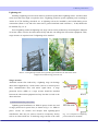
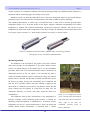
Download FluxHandbook_Ver1.0a

Practical Handbook of
Tower Flux Observation
Editorial Board of
"Practical Handbook of Tower Flux Observation"
Editorial Board
Editorial Board
Chairman
YAMANOI Katsumi (Hokkaido Research Center, FFPRI)
Members (in alphabetical order)
HIRATA Ryuichi (Faculty of Agriculture, Hokkaido University)
KITAMURA Kenzo (Department of Meteorological Environment, FFPRI)
MAEDA Takahisa (Institute for Environmental Management Technology, AIST)
MATSUURA Shoji (NILGS)
MIYAMA Takafumi (Kansai Research Center, FFPRI)
MIZOGUCHI Yasuko (Hokkaido Research Center, FFPRI)
MURAYAMA Shohei (Institute for Environmental Management Technology, AIST)
NAKAI Yuichiro (Department of Meteorological Environment, FFPRI)
OHTANI Yoshikazu (Department of Meteorological Environment, FFPRI)
ONO Keisuke (Agro-Meteorology Division, NIAES)
TAKAHASHI Yoshiyuki (Center for Global Environmental Research, NIES)
TAMAI Koji (Department of Soil and Water Conservation, FFPRI)
YASUDA Yukio (Tohoku Research Center, FFPRI)
Secretary
MIZOGUCHI Yasuko (Hokkaido Research Center, FFPRI)
YUTA Satoko (Department of Meteorological Environment, FFPRI)
Matsunosato 1, Tsukuba, Ibaraki, 305-8687 JAPAN
Department of Meteorological Environment
Forestry and Forest Products Research Institute (FFPRI)
Phone: +81-29- 873-3211 (main)
E-mail: [email protected]
i
Practical Handbook of Tower Flux Observation (Ver. 1.0)
Preface
Efforts to mitigate global warming at the societal level call for a rapid implementation of systems that quantitatively
evaluate the carbon dioxide (CO2) budgets for forests, croplands, grasslands, and other terrestrial ecosystems. For
observational studies of carbon budgets for terrestrial ecosystems, tower-based micrometeorological CO2 flux
observations conducted at the interface between the atmosphere and terrestrial ecosystems have attracted attention as an
approach that allows direct measurements of the amount of CO2 absorbed by the terrestrial ecosystems from the
atmosphere. Such CO2 flux observations have been taking place at more than 200 locations worldwide. Furthermore,
efforts to integrate studies from tower-based observations on CO2 and energy fluxes and those on the carbon dynamics
and energy budgets of terrestrial ecosystems are currently in progress with the goals of improving the parameterization
of ecosystem models relevant to global warming research and elucidating the influences of natural and anthropogenic
disturbances, e.g., typhoons and land use changes, respectively, on the dynamics of diverse terrestrial ecosystems.
With this background, four research institutes (Forestry and Forest Products Research Institute, National Institute for
Agro-Environmental Sciences, National Institute of Advanced Industrial Science and Technology, and National Institute
for Environmental Studies) which have conducted long-term tower observations within Japan agreed to conduct joint
research and development in 2007 in order to promote shared use of observation data, for which the reliability has been
ensured and quality-control has been performed. The observation data under consideration concern exchanges of energy
and mass such as CO2 between terrestrial ecosystems and the atmosphere, the exchanges for which worldwide
observation networking has been promoted. A micrometeorological observation and analysis technique called the eddy
covariance method has become very common in recent years as a result of the development of measuring instruments
with a relatively high response time and improvements in computational processing speed. This technique has enabled
continuous acquisition of ecosystem production data as well as ecosystem-atmosphere mass and energy exchange (flux)
data, without damaging the ecosystem under observation. Data acquisition with the eddy covariance method has, in turn,
allowed clear evaluations of the diurnal, annual, and inter-annual variations of energy and mass (e.g., CO2) exchanges,
contributing significantly to improved understanding of ecosystem carbon dynamics and energy budgets.
Unlike general surface observations of meteorological variables, the micrometeorological technique does not require
uniform conditions for the observation site and instrumentation. Therefore, while the micrometeorological technique
offers various advantages, the data acquired with this technique have been subject to measurement uncertainties
associated with variations in the observation location, observation method, and analysis method since the initial
adoption of this technique. Currently, the observation-data sharing that has been promoted by FLUXNET, AsiaFlux and
other related programs aims to inter-compare data through direct means or through indirect means such as model
validation and also to achieve an improved understanding of the regional-scale carbon budget. Therefore, great care has
been taken in order to eliminate data uncertainties including those associated with the use of the micrometeorological
technique. For example, in Europe and Canada, instrumentation and analysis techniques have been standardized by
creating manuals since the beginning of the observational efforts (Aubinet et al., 2000; Fluxnet-Canada, 2003), and
tower observations have been implemented in a systematic manner. In Japan, under the leadership of the AsiaFlux
Steering Committee, “Current Practice of CO2 and Other Flux Observations in Measurements for Terrestrial
Ecosystems“ (AsiaFlux Steering Committee (ed.), 2003 in Japanese, 2007 in English) was published, which has
ii
Preface
contributed to the improvement of observation and analysis standards and the establishment of an observation network
by illustrating measurement and analysis techniques. In 2004, with FLUXNET as the nucleus of the project, a handbook
with details on a wide variety of topics including the theory and technique of observation and analysis and examinations
of factors affecting observation error was published (Lee et al. (ed.), 2004). With the manual and the handbook, a
guideline has been created for handling factors which cause uncertainties in observation data. On the other hand, of the
issues associated with uncertainties in observation data, errors induced by phenomena that depend heavily on the terrain
conditions of the observation site, e.g., complex terrain, are fundamental causes of uncertainties in observation data and
are rooted in the principle of measurements and analysis. This issue remains as a research topic which needs to be
continuously addressed.
Accordingly, the number of literature references on observations by the eddy covariance method has increased
compared to the time when such observations were initiated. However, when observations and analyses by the eddy
covariance method are attempted in practice, detailed technical information that is not described in the existing
publications becomes necessary for many of the tasks associated with the project such as starting a new observation site,
deployment of the observation system, and analyses and quality control of the data. Given this circumstance, it has been
proposed that data quality and distribution among researchers be increased by making the necessary technical
information available on the internet and allowing researchers, who are aware of the necessity of standardizing the data,
to share technical information. This proposal aims to contribute to the construction of a system that provides an
improved estimate of the amount of CO2 absorbed by terrestrial ecosystems, which is relevant in the mitigation of
global warming. In the regions centered around Asia, tower-based observation sites within terrestrial ecosystems to be
used for the purpose of validating various models remain scarce. Without detailed technical information such as that
provided in this manual, it may be nearly impossible for a research team to start and operate a new observation site
alone.
Because detailed technical information such as that described above is inseparably linked to the development of
observation and analysis techniques, this information has been made available on the internet, which allows for
relatively easy update of information – an advantage of the internet. Because the information included in this manual is
published on paper at this time, the inability to easily update the information is one of the biggest concerns. Nonetheless,
publication of the present manual is valuable in that it provides a record of the current state of observations and analyses
from a technical point of view. It is our hope that the present manual will serve in transferring various techniques to the
science communities in Asia and contribute to the efforts to mitigate global warming through the expansion of tower
observation
August 2011
OHTANI Yoshikazu
Director, Department of Meteorological Environment,
Forestry and Forest Products Research Institute
iii
Practical Handbook of Tower Flux Observation (Ver. 1.0)
Preface to English edition
A half century ago, Dr. Eiichi Inoue, a pioneering scientist of turbulence in the atmospheric boundary layer and
famous for his studies on “Honami” (waving plants), tried to measure carbon dioxide (CO2) fluxes over crop fields by
applying the aerodynamic method. He dreamed that a sensor similar to a heat flux plate could be developed in the future
(he named the sensor the CO2 flux plate), and that by merely setting the plate horizontally we could easily measure the
CO2 flux from the difference between the concentration of CO2 at the upper side of the plate and that at the lower side
of the plate. We may say that his dream “partially” came true with the development of the eddy covariance system
consisting of a sonic anemometer, a fast-response infrared gas analyzer, and a data logger. Now, the eddy covariance
system is used for monitoring fluxes of CO2 as well as those of water vapor and sensible heat in various terrestrial
ecosystems throughout the world.
However, the measurement of CO2 flux using the eddy covariance system is not as easy as, and actually far different
from that using the CO2 flux plate which Dr. Inoue dreamed of a half century ago. It is certain that open- and
closed-path infrared gas analyzers as well as sonic anemometers and data loggers have recently been much improved
and have become more sophisticated so that we can operate those advanced instruments more easily than two decades
ago. In addition, as the number of users of the eddy covariance system increases, manufactures and their agents are
providing detailed instruction manuals, technical notes, and even training courses. However, these resources are not
enough for someone who is going to start flux observations using the eddy covariance system because these materials
and activities generally focus on how to use the individual instruments or the eddy covariance system at best, but do not
discuss practical issues related to eddy covariance flux observation such as constructing an observation site including a
tower and related facilities, setting up the eddy covariance instruments in the field, and conducting the
micrometeorological observations that are inseparable from the eddy covariance flux observations. AsiaFlux has also
had several training courses including lectures on the theory of flux observation, but could not spend much time on the
above-mentioned practical issues, which are really required for newcomers, especially those without expertise in
micrometeorology.
As shown by its title, the “Practical Handbook of Tower Flux Observation” focuses on the practical issues in eddy
covariance flux observation and includes a substantial amount of useful knowhow and unique sections such as
“lightning surge countermeasures” and “detection and reduction of noise”, which are rarely found in similar
publications. All of the authors of this handbook have been engaged in long-term flux monitoring in forest or cropland
sites and have expertise in eddy covariance flux observation. I sincerely appreciate the efforts of the authors to spend
their valuable time to share their experiences and knowhow with the readers, and expect this handbook to be utilized as
a practical reference by eddy covariance users and in training courses on eddy covariance flux observation. It is also my
hope that another practical handbook, which focuses on the processing of eddy covariance data and is complementary to
the present handbook, will be published in the near future.
August 2011
MIYATA Akira
Director, Agro-Meteorology Division,
National Institute for Agro-Environmental Sciences
iv
Preface
v
Practical Handbook of Tower Flux Observation (Ver. 1.0)
Contents
Editorial board ····················································································································· i
Preface ····························································································································· ii
Preface to English edition ········································································································ iv
1. Observation Planning and the Selection of Flux Observation Sites
1.1 The observation site ···································································································· 2
1.2 Building infrastructure ································································································· 5
1.2.1 Obtaining land-use permission ··············································································· 5
1.2.2 Tower construction and maintenance ······································································· 7
1.2.3 Electric power supply ························································································ 11
1.2.4 Lightning surge countermeasures ···········································································14
1.2.5 Observation hut ·······························································································18
1.2.6 Other ············································································································19
1.3 Measurement variables: recommendations and precedence ·····················································21
1.3.1 Variables essential for eddy covariance flux measurement (turbulence fluctuation method) ······21
1.3.2 Micrometeorological and hydrological elements ·························································21
1.3.3 Structure and basic characteristics of a plant canopy ····················································23
Related information for chapter 1 ·······················································································25
2. Observation of Turbulence
2.1 Ultrasonic anemometer thermometers (SATs) ····································································28
Appendix 2.2-1: Sample program ·················································································40
2.2 Open-path CO2/H2O gas analyzers ·················································································41
2.2.1 Measurement of fluctuating CO2 concentration by an open-path gas analyzer ······················41
2.2.2 Measurement of fluctuating H2O concentration by an open-path gas analyzer ······················56
2.2.3 Recent progress in addressing the effect of surface heating of open-path analyzers as of 2011 ····59
Appendix 2.2-1: Serial number-specific characteristics of the LI-7500 (LI-COR, Inc., U.S.A.) ·········63
Appendix 2.2-2: High frequency flux loss ·······································································64
Appendix 2.2-3: The influence of heating by the open-path gas analyzer on flux calculation ···········64
Appendix 2.2-4: Issues associated with horizontally deployed open-path gas analyzers ··················65
Appendix 2.2-5: Influence of dirt and dust accumulated on the lenses of the open-path gas
analyzer on CO2 number density measurements ···········································65
Appendix 2.2-6: Density and mixing ratio ·······································································65
Appendix 2.2-7: Literature which reports a negligible effect of instrument surface heating on
open-path analyzer measurements ···························································66
2.3 Closed-path CO2 gas analyzers ······················································································67
Appendix 2.3-1: References on corrections for high-frequency signals ·····································85
vi
Contents
2.4 CO2 storage change ···································································································86
2.5 Relaxed eddy accumulation (REA) method ·······································································96
2.6 Data logger ··········································································································· 103
2.7 Detection and reduction of noise ·················································································· 106
Related information for chapter 2 ····················································································· 109
3. Micro-meteorological Observation
3.1 Radiation ············································································································· 116
3.1.1 Solar radiation ······························································································· 116
3.1.2 Longwave radiation ························································································· 119
3.1.3 Net radiation ································································································· 122
3.1.4 Photosynthetically active radiation (photosynthetic photon flux density) ·························· 124
Appendix 3.1-1: Necessary factors to obtain the solar position ············································· 128
Appendix 3.1-2: Conversion of measurement units ·························································· 129
3.2 Wind direction / wind velocity ···················································································· 130
3.3 Air temperature ······································································································ 135
Appendix 3.3-1: Unit conversion ················································································ 141
3.4 Humidity ·············································································································· 142
Appendix 3.4-1: Definitions of humidity ········································································ 145
Appendix 3.4-2: Equilibrium relative humidity of air with chloride-saturated solution ·················· 146
3.5 Soil temperature and soil heat flux ················································································ 147
3.5.1 Soil temperature ····························································································· 147
3.5.2 Soil heat flux ································································································· 149
3.6 Soil moisture ········································································································· 152
3.7 Precipitation / snow water equivalent (SWE), snow survey (snow depth, snow weight) ················· 156
3.7.1 Precipitation (rainfall/snowfall) ··········································································· 156
3.7.2 Snow survey (snow depth, snow weight) ································································ 158
3.8 Water level, water temperature, irrigation and drainage ······················································· 160
3.8.1 Water level ··································································································· 161
3.8.2 Water temperature ··························································································· 162
3.8.3 Irrigation and drainage ····················································································· 163
3.9 Data logger ··········································································································· 166
Related information for chapter 3 ····················································································· 168
Literature cited ······················································································································································· 177
List of symbols ·················································································································· 184
Index ····························································································································· 188
List of authors···················································································································· 194
vii
Practical Handbook of Tower Flux Observation (Ver. 1.0)
viii
Observation Planning
and the Selection of
Flux Observation Sites
Practical Handbook of Tower Flux Observation (Ver. 1.0)
Chapter 1
1.1 The observation site
This section describes how to select appropriate sites for performing long-term, continuous
observations of energy and CO2 fluxes.
Basic concept
When selecting a site, you must clarify the purpose of your proposed observation by answering the
question: In what type of ecosystems will these flux measurements be taken? Specifically, you must
determine the following required conditions beforehand: vegetation type (dominant species), density,
height, and age; climatic conditions; soil characteristics; potential disruptions in the ecosystem due to
natural causes; and potential disruptions in the ecosystem because of man-made changes such as tree
trimming or land development. Then, search for an appropriate observation site based on these variables.
Careful site selection is important as it can profoundly affect the validity of your observational data;
preliminary studies on possible observation sites are worthwhile.
Flux measurements performed using the eddy covariance method postulate fewer atmospheric or
land-surface condition as compared to those performed using other micrometeorological methods.
However, the eddy covariance method does require that there is a flat terrain and homogeneous vegetation
in the windward side of the observation point (Schmid, 1997).
Preparation
Select candidate observation sites based on information collected from the following: topographic
maps, vegetation maps, aerial photography, satellite images, land use maps, forest management maps, data
on climate and hydrological conditions, and history of land use and management. With respect to climatic
conditions, studying the speed and direction of prevailing winds and changes in their daily and seasonal
patterns helps to determine the most appropriate site for flux measurements and sensor positioning.
Practically, it is necessary to collect information on land ownership, land-use rights, and building
restrictions. It is also important to find out the social structure and security of the area from people who are
familiar with the surrounding region. At the same time, draw up an observation plan that specifies the
observation period, methods for managing vegetation, manpower requirement, methods employed for data
collection, data usage, and procedures for making the data publically available, as well as any relation
between your study and other flux observation studies.
2
1.1 Selection of flux observation sites
Tips!
Flux measurement studies require two full-time staff members for each observation site (Baldocchi et
al., 1996). Additional staff members are required for the measurement of other items such as
micrometeorological variables. Advances in measurement equipment have reduced the need of
maintenance, and thus number of staff. Even then, it is better to avoid working alone in high places on a
tower.
Tips 1.1-1
Selecting a flux measurement point
When candidate sites have been identified, you should reconnoiter them, and if possible, view them
from above. Select an appropriate observation point (to set up a tower or pole) and ensure that there is a
vast expanse of flat terrain and homogeneous vegetation on its windward side. It is desirable to set the flux
measurement height at least twice as the vegetation height. However, due to technical limitations and
micrometeological-footprint restrictions (see section that contributes to the observed flux: 1.2.2, “Tower
construction and maintenance”), the height of the flux measurement might be lowered in some instances.
Avoid areas that have artificial facilities, such as buildings and power transmission lines or areas that
have cars and other traffic facilities nearby. This is because gas emissions from traffic and electrical noise
can invalidate your observational data. It is ideal to have an areal allowance of the same ecosystem for
conducting ecological and pedological surveys, which would disturb vegetation and soil but without
affecting flux observation. In most of the Asian countries, it is not rare that agricultural areas other than
permanent grasslands are managed in sections of one hectare or less. Each section may use a different
management method, and this can have an adverse effect on the observation results. It is important to take
this factor into consideration when conducting a preliminary survey on an observation site.
Access
It is desirable that there is a road leading to the observation tower so that heavy equipment can be
carried into the tower for maintenance. Where there is no road, one should be built, or if it is difficult to
build a road because of strict restrictions on the use of roads or due to steep slopes, installing a monorail is
a good option. However, since emissions from vehicles can adversely affect observation results, it is
necessary to have some restrictions on traffic.
Remote site
There are some areas that are difficult for people to access, but they must be observed as they are
considered important ecosystems. We call an observation site installed in such an area as a “remote site”.
What steps must be taken to conduct a long-term survey at such remote sites? It is impossible to install
commercial power lines in such locations. Access is also extremely inconvenient. To enable observational
3
Practical Handbook of Tower Flux Observation (Ver. 1.0)
Chapter 1
studies in such an area, we should first plan how to
address problems with the living environment, such as
problems
relating
to
transportation
and
accommodation.
Obtaining the cooperation of local residents is also
essential for conducting a successful study. Prior
preparation is ideal as it ensures that many obstacles
are removed before the study begins. Continuous
year-round observation is ideal in principle, in many
cases however, that is not always possible due to
Photo 1.1-1 A supportive year-round weather
limited budgets, human resources and electric power
station. (Tura, Russia)
supply. In such case, we should reduce the number of
observation items and the duration of observation to secure the indispensable data. Moreover, it is
desirable to set up an additional weather station in a readily accessible location where security and electric
power for collecting supportive meteorological data throughout the year (Photo 1.1-1).
4
1.2 Building infrastructure
1.2 Building infrastructure
This section describes some public procedures of the government, with cases of Japan as examples.
When setting up an observation station in other countries, it is necessary to proceed corresponding each
local or national government.
1.2.1 Obtaining permission for land use (example of case in Japan)
Private land
It is difficult to provide a general explanation of the procedures involved in acquiring permissions for
land-use for studies that include the construction of towers or roads on private land. It is necessary to
discuss the procedures with the land owners, and also, be sincere and patient in all your dealings with them.
While proceeding with the procedures for acquiring permission for land use, you should begin the
necessary construction and survey work. If the observation site is situated in an area designated as a
national park, a protected forest, or an erosion control area, then you need to obtain permission from the
proper authorities to use the land. (Details are explained below.)
Agricultural land
When you set up an observation station on an agricultural land, you must first obtain permission from
the land owner to use his land for the study. Towers tend to be rather small when built on agricultural lands,
compared to these in forest, and the impact of tower and facilities on cultivation should not come to an
issue. However, constructing objects such as towers in the middle of fields can adversely affect the
efficiency of agricultural work (especially work done by tractors and machinery). When negotiating the
rent with the land owner, this point should be taken into consideration.
Although installing a tower in an agricultural field rarely affects the surrounding fields, the consent of
neighboring land owners must also be acquired for managing the observation site. The consent can be
acquired through a land improvement organization or other local organizations. It is always important to
maintain amicable relation with neighboring land owners as they might also provide information that is
useful for your study.
Special areas and specially preserved areas in national parks and quasi-national parks
When you set up an observation station in special areas and in specially preserved areas of national
parks or quasi-national parks, you need to obtain permission from the proper authorities. For a national
park, obtain permission from the Environment Minister; for a quasi-national park, obtain permission from
the Prefectural Governor (Articles 13 and 14 of The National Parks Act). The installation of facilities is
5
Practical Handbook of Tower Flux Observation (Ver. 1.0)
Chapter 1
strictly regulated in these areas, and it is therefore, difficult to build a tower larger than the simple one such
as shown in Photo 1.1-1.
National and public forests
When the observation tower or roads used to access the research site are part of a national forest, you
need to obtain a Permit for Using National Forest for entering the forest. First, visit the local forest
management office and forest administrative bureau for applying to obtain permission to use the forest and
start negotiating with them sincerely. For land use activities that entail observations to be made as part of a
public research project, you can collaborate with public research organizations by following the procedures
outlined in the Implementation Guideline for Technical Development of Forest Office and in this case no
land use fee will be charged. Instead you will be obliged to submit annual reports on the implementation of
technical development. With regard to the use of forests owned by prefectural governments and other
municipalities, the process of obtaining permission varies from community to community. Some local
governments have systems that allow for land lease and prefectural forest use. Contact the division in
charge of forests and follow the necessary procedures. If the target forest is designated as a protected forest
or an erosion control area, then you need to acquire a protected forest work permit or an erosion control
work permit just as you would have done for the use of private land.
Protected forests
When large-scale construction and other work are to be performed in a protected forest area, you can
file a petition for the designation of the protected forest to be cancelled. To apply for such cancellation,
either of the following two conditions is required: when no reason can be found for the forest to be
designated as a protected area, or; when the outcome of research will be significant in terms of public
benefit, and will be more important than the protection of the forest. In reality, however, there is only a
slight chance that any such application will be accepted, even if it meets the requirements outlined above.
So, when you undertake a small-scale observational study in a protected forest, you need to apply for a
permit, register the observation tower and cabin as temporary buildings, and obtain a permit to cut down a
few trees (a protected forest work permit).
Erosion control area
The need for observations is not among the reasons for the designation of an erosion control area to be
cancelled. It is also virtually impossible to build permanent buildings in a location that is designated as an
erosion control area. This also applies to rivers. Building facilities or roads in an area that has been
designated as an erosion control area under The Sand Control Act or alongside rivers that have been
defined as rivers by The River Act is extremely difficult. However, it is possible to obtain permission to
construct a few temporary buildings in these areas not by obtaining a Construction Permit, but by
obtaining an Action Permit in an Erosion Control Area and River.
6
1.2 Building infrastructure
Tips!
To renovate a boardwalk or an observation station located in a protected forest or in an erosion control
area, you must apply for the permits stated above each time. Please remember this when you plan to
make large-scale repairs.
Tips 1.2-1
Tips!
Although an observation facility is usually temporary, The Building Standards Law requires you to
obtain a construction certificate if you intend to use it for a long time period. Besides obtaining land-use
permissions, confirm whether you need to obtain a permit for building a tower and an observation house
and if required, follow the necessary steps for obtaining these permits.
Tips 1.2-2
1.2.2 Tower construction and maintenance
Height
The specifications of a tower for flux observations between the atmosphere and ecosystem in forests,
grasslands, or agricultural lands are determined by the construction budget and on-site conditions however,
the tower must be at least higher than the surrounding vegetation. There have been cases (e.g., Laubach et
al., 1994) where measurements taken from observation points that were 3 % higher than the surrounding
vegetation were not very different from those taken from observation points that were 50 ~ 70 % higher
than the surrounding vegetation. Thus, observations are possible at any height provided the observation
site is slightly higher than the surrounding vegetation. However, measurements taken at a lower site tend to
be influenced more strongly by the surrounding vegetation. So, it is necessary to check whether the
observed values are representative of those of the surrounding vegetation. Footprint analysis prior to
observation is an efficient means of verification (e.g., Schuepp et al., 1990; Rannik et al., 2000; Kormann
and Meixner, 2001; Okada, 2002). However, along with such ex ante analysis, it is recommended that site
inspections be performed at various observation heights (depending on on-site conditions). In such cases,
the tower must be higher than the surrounding vegetation with a certain allowance. Also, if long-term
observations are performed at a height close to the vegetation height, then the vegetation will grow and
approach the measurement level. Therefore, when a tower is constructed, its height should at least be 1.5 ~
2 times that of the surrounding vegetation, regardless of the height of the flux observation equipment.
Tower types and features
In grassland or agricultural areas, a pole-like tower of approximately 3 ~ 5 m is used in most cases
7
Practical Handbook of Tower Flux Observation (Ver. 1.0)
Chapter 1
(Photo 1.2-1). There is a free-standing type of tower,
which has a pipe driven deep into the ground; a
reinforced type that is supported by wires; and a tripod
type.
In a forest, a higher tower is needed. Most
common type is the one which the observer can
climbs up with the instruments. Some of the towers
have stairs (Photo 1.2-2; here we call it a “scaffolding
tower”) and others have ladders (Photo 1.2-3; here we
call it a “ladder tower”). There is also another tower
Photo 1.2-1 A pole-like tower. (Mase paddy
type with an elevating table attached to lift up the
flux site)
instruments to the top.
The advantage of using a scaffolding tower is that it is easy to ensure the safety of the climber. It is also
easier to go up and down the stairs when holding an instrument in hand. So the installation and
maintenance of instruments is comparatively easy, even when there are few observers.
In case of a scaffolding tower, a four-sided tower is built on a comparatively broad yet shallow
foundation, with metal stays that extend outward from the four corners of the tower and are fixed to the
buried concrete anchor. An anchor is important for ensuring adequate protection against strong winds, so
sometimes a large anchor is buried deep in the ground (e.g., an anchor of more than 1 m3 is buried at a
depth of more than 1 m). In snowy areas, where snow load such as weight on the metal stays and settling
force can be significant, a scaffolding tower without stays is possibly chosen. In such cases, it is necessary
to have a large base area and to use reinforcing materials that are selected on the basis of their strength to
withstand the snow season.
A scaffolding tower that uses ordinary scaffolding pipes and clamps is treated as a temporary
construction at a general construction site, whereas a tower used for long-term observation must have an
appropriate distribution of stiffened elements, based on specifications such as the tower height, and it
should be designed and constructed using strength calculations based on the planned height of the tower
and properties of the construction materials. From the perspective of construction and maintenance, using
strong, lightweight materials (such as aluminum) is preferable, but the material costs rise steeply.
Many ladder towers consist of triangles (or quadrilaterals) of about 10 cm on one side (Photo 1.2-3).
These towers are used for radio and cell phone communications, and materials and strength calculations
are often set as standards. Since telecommunication towers are used around the world, it is easy, even in
overseas, to construct such a tower as it can be built relatively cheaply according to the local labor costs. It
is also possible to add an optional electric or manually operated winch or space for working and evacuation,
which is called a safety box or stage. However, this type of tower requires greater physical strength of the
observer for moving up and down the tower compared with the scaffolding tower. Also, when working at
great heights, the sensation of being high above the ground is more intense, and this will limit the number
of people who can work in such an area. It is also difficult to move up and down while holding something,
8
1.2 Building infrastructure
so to set up an instrument you need a pulley and a rope as well as a support person on the ground. A device
for preventing falls when working high above the ground or safety gear used for mountain climbing is
indispensable for moving up and down this type of tower. Moreover, setting up metal frames that are used
for climbing greatly reduces the worker’s sense of fear when installing and removing safety appliances.
This type of tower stands like a rod on a base, whose area is relatively small with respect to its height. So,
when it is used for long-term observations its foundation should be laid very deep in order to prevent it
from falling over. Also, it is possible to build this type of tower, depending on the height, as a self-standing
tower without the use of stays. However, when the height of the tower greatly exceeds the top of the forest
canopy, metal stays and an anchor of appropriate size are required.
Photo 1.2-2 “Scaffolding tower” with access
Photo 1.2-3 “Ladder tower” with a ladder-like part
stairs. (Kahoku Experimental Watershed)
for easy access. (Kampong Thom Province,
Cambodia. Photograph: courtesy of Shimizu Akira)
Photo 1.2-4 Monorail used for transporting construction materials.
(Yamashiro forest hydrology research site)
9
Practical Handbook of Tower Flux Observation (Ver. 1.0)
Chapter 1
Transporting construction materials
Since usually a high tower is constructed in a forest and most of the construction work is done in the
mountains, the transport of construction materials is arduous. Use a monorail to effectively transport
materials in large amounts while minimizing damage to the forest floor (Photo 1.2-4). The price of a
monorail car is about three million yen, and the costs of laying the rail is about 30 ~ 40 thousand yen per
meter.
Tower maintenance
Maintenance of an observation tower is essential to ensure that observers working at the tower are safe.
If a tower is constructed with a strong foundation, using materials that have been chosen based on suitable
calculations of their strength, it can last for more than ten years unless damaged by a natural disaster.
However, even when it does not experience strong winds or a severe earthquake, the tension in the stays of
a tower will change slightly because of vibrations caused by wind and the observer’s movements on the
tower. It is thus preferable to measure the tension of the stays once a year, using a tension meter, and to
adjust the tension based on these measurements. It is also necessary to constantly check for corrosion of
the metal joints on the tower and to replace them when necessary by ordering the parts from a supplier or
by contacting the tower builders.
Especially for a tower built in a forest, even if the tower itself is designed to sustain vibrations induced
by strong winds, it is conceivable that a tree could fall on the tower or on the stays and cause severe
damage. To prevent this, any tree that could potentially interfere with the tower or the stays should be cut
down. In a forest with a fully closed canopy, cutting down a single tree creates a gap in the forest, but the
influence on the observational results appear to be small (e.g., Kelliher et al., 1995). If many trees need to
be felled, there are concerns that labor for cutting and transporting them will be considerable and that the
habitat will change. Instead of cutting trees, it is recommended that the target trees be tied to other trees
with a steel wire (Photo 1.2-5). Trees that are tied together do not fall as easily as single trees and the risk
of their causing damage to the tower or to the stays is also much lower. The Kahoku Experimental
Watershed of the Forestry and Forest Products Research Institute was hit twice by typhoons with
Photo 1.2-5 Trees connected by steel wires at the base (left) and at 10 m (right). The red arrows show the
connections. (Kahoku Experimental Watershed)
10
1.2 Building infrastructure
maximum wind velocities of 50 ms–1, but none of the trees that had been tied together fell and so there was
no damage to the tower or the stays and the observations can be continued without interruption.
At an observation site located on an agricultural land, agricultural work such as crop planting,
harvesting, and cultivation is conducted (mostly by machines) several times in a year. These alter the
ground surface conditions. A tower built on an agricultural field can interfere with agricultural work, but
observations of upward radiation, soil heat flux, plant community profile, and so on are often carried out in
the vicinity of the tower, so it is important to ensure the homogeneity of the land, even in the vicinity of the
tower. There are two ways to do this: One is to carry out observations by setting up a simplified tower that
can be easily transported (such as a tripod) and pulling down the tower temporarily when there is
agricultural work to be done; the other is to carry out observations at the permanently installed tower after
asking the field administrator to avoid agricultural work around the tower and having the observers
themselves do the agricultural work manually in the vicinity of the tower. Even when the latter option is
chosen, it is better to pull down the tower once in several years to ensure cultivation of the entire
agricultural field.
1.2.3 Electric power supply
Commercial power supply
Wherever possible, the use of a commercial power supply is recommended as is the introduction of a
facility that has considerable capacitance. A back-up power supply should be maintained for the event of
power loss, and the observation system should have automatic data saving and power restoration features.
To install a commercial power supply at the newly set-up experimental site, certain steps have to be
followed by an electrical contractor who is affiliated with the power company based in each region. For
example, Kandenko Co., Ltd in the region around Tokyo. Locally registered electricians can be recruited
through the local office of the power company in each region. If there are residential area close to where
power is to be installed, setting up the power supply can be done free of charge for a certain distance from
such area. When a meteorological observation tower is installed, it is often several kilometers away from
the residential area, there will be indispensable expenses for its installation, including the installation of
electric poles and electric wires. Rental expenses will accrue when electric poles are present on private
land.
Tips!
Comprehensive discussions with personnels of an electrical engineering company affiliated with a
power company can greatly improve their support level. It is important to emphasize the public nature of
observations, taking the time and making the effort to provide an explanation for your activities and to
participate in negotiations on-site prior to beginning your study.
Tips 1.2-3
11
Practical Handbook of Tower Flux Observation (Ver. 1.0)
Chapter 1
When installing a power supply line, high voltage electric power lines should be laid as close as
possible to the observation tower or to the experimental site in the forest, and a transformer should be set
on the nearest electric pole. This avoids problems such as power line noise after the start of the observation,
and it also makes it easy to change the capacitance.
As for wiring in a forest, in order to prevent the wire from being cut or damaged by falling trees, the
power supply line should be laid on or under the ground after being placed into protective tubes. (Products
such as corrugated pipe, accordion pipe, and so on can be used.) If a power supply line is laid under the
ground, then maintenance after setup is difficult. It requires efforts such as setting up a linkage box
midway along the line. As for wiring on telephone poles, it may be necessary to cut down some trees so
that they do not touch wires (Photo 1.2-6). When conservation of the forest is a priority, it is better to
install the power supply line on or under the ground. When the situation allows, “unfixed wiring” on the
ground, using protective tubes, is favorable for maintenance (Photo 1.2-7).
When the location is isolated and a commercial power supply is unavailable, a dynamo or a power
generation system employing solar panels can be used. Nowadays, many observation sites use a
photovoltaic generator based on solar panels. When a dynamo is used, it should be installed in such a
position that its exhausts do not affect flux observations.
Photo 1.2-6 Aerial wiring in a forest.
Photo 1.2-7 Unfixed wiring. The forest floor
(Yamashiro forest hydrology research site)
undulates, so it is more practical to use underground
corrugated protective tubes for unfixed wiring.
(Yamashiro forest hydrology research site)
12
1.2 Building infrastructure
Tips!
When a high voltage electrical power line cannot be extended to the transformer of the utility pole near
the observation facility, long-distance power transmission is needed between the transformer and the
observation facility either with an AC 100 V line or with a 200 V single-phase three-wire system. In this
case, the resistance of the wire extending to the observation facility can cause a voltage drop. As a
result, depending on the electric power required, sufficient power-supply voltage may not be available
for conducting observations. Use of a wire with small conductor resistance (i.e., a thick wire) helps to
minimize the voltage drop. Many measuring instruments that operate normally at 95 V perform unstably
at 90 V though the degree of instability depends on the individual measuring instrument. Therefore, the
voltage of the AC power supply that is to be used for the observation system needs to be checked.
Tips 1.2-4
Electric power generated by a photovoltaic power source
Photovoltaic cells on solar panels charge batteries using sunlight. During sunshine hours, a
photovoltaic generator generates more power than what the observation system needs, and the surplus is
used to charge the battery. The charged power is consumed during the night or during non-sunshine hours.
A charge controller is used to prevent the battery from overcharging and also prevents excessive discharge.
In terms of the charging capacity and durability of the battery, it is most appropriate to use a deep cycle
battery as it can be used even when fully charged, and it also delivers a consistent voltage as it discharge.
The capacity of the solar panel and the battery depend on power consumption by the observation system
and on the amount of available solar radiation. For more
information on how to calculate capacity, please refer to the
technical data posted on related websites. The available electric
power is limited. The observation system should have low
power consumption itself, and equipped with automatic power
control functions including saving of on-memory data, turning
off low-priority devices for power saving, and restarting of
observation.
The main precautions to take when using solar panels are as
follows: 1) solar panels should be used so that the wind impact
on the flux sensors is minimized; 2) the wind resistance of the
panel is high, so care should be taken that the tower or the panel
is not blown away by the wind; 3) the electrical resistance of
wiring should be small and loss of power should be minimized;
and 4) care should be taken to avoid electric shocks caused by
13
Photo 1.2-8 A flux observation tower
using solar cells. (Tura, Russia)
Practical Handbook of Tower Flux Observation (Ver. 1.0)
Chapter 1
the electric current in the panel. Measures such as light shielding should be taken when work is performed
in the vicinity of the panels. An example of a flux observation tower using solar cells is shown in Photo
1.2-8.
Tips!
When a lead storage battery becomes overly discharged, the precipitated lead sulfate forms hard crystals
on anode of the battery. This is called sulfation, and these crystals have a low solubility, which makes it
practically impossible to recharge the battery. Deep-cycle batteries are the same, because they are lead
storage batteries in principal. However, their electrode are strengthened to make them more discharge
resistant than ordinary lead storage batteries.
Tips 1.2-5
Tips!
Solar panels should be set up to achieve the maximum possible production of electricity. Sun’s rays
should preferably hit the panels at a right angle, but since the sun’s angle changes daily and seasonally,
solar panels are usually set at an angle of 10 ~ 40 degrees facing south (north in south hemisphere). The
influence of surrounding obstacles on the panels is taken into account as well as the influence of the
panels themselves on flux observations.
Tips 1.2-6
1.2.4 Lightning surge countermeasures
Lightning damage on tower observations
Since lightning tends to strike tall, pointed objects, observation towers are prone to lightning strikes.
Electric current (lightning surge) generated by lightning momentarily produces a large current and a high
voltage, and these can damage observation facilities. There are two kinds of surges: a direct lightning surge
caused by direct strikes on a tower; and a lightning-induced surge caused by strikes on the surrounding
area. Both cause damage that can include destruction and breakdown of electronic observation equipment.
Surges caused by direct lightning strikes generate a particularly large amount of energy and they can cause
severe damage, including fires.
For flux observation facilities, installation of lightning protection equipment is required by law when
the facility is first established and additional measures can also be taken to ensure the protection and safety
of observation equipments. The former includes installing a lightning rod on an observation tower, and the
latter includes protecting power lines, communication lines, and sensor signal lines.
14
1.2 Building infrastructure
Lightning rod
Installing a lightning rod is the most effective protection against direct lightning strikes. An observation
tower more than 20 m high is required to have a lightning protection system (lightning rod) according to
Article 88 of The Building Standards Act. A lightning rod can be installed by the builder during tower
construction (Photo 1.2-9) and at the same time a ground with little earth resistance (< 10 Ω) should also
be installed (Fig. 1.2-1).
Even if lightning strikes the lightning rod, surge current can be produced by electromagnetic induction
in various cables wired to the observation facility and this can damage the observation equipment. Thus,
surge arresters are required even if a lightning rod is installed.
Photo 1.2-9 A lightning rod (left) and a ground (right) installed in an observation tower.
(Sapporo forest meteorology research site)
Surge arrester
Abnormal current flow induced by a lightning surge can damage
observation equipments by various routes (such as via electric power
lines, communication lines, and sensor signal lines). A surge
protection device (SPD) or a surge arrester should be installed
between the observation equipment and any line that is wired to the
observation hut.
Countermeasures for power lines
Lightning-proof transformers or SPDs in power circuits are used
as surge protectors for power lines, as shown in Fig. 1.2-1. SPDs in
power circuits are smaller and cheaper than lightning-proof
transformers; thus, they are easier to install in a temporary facility
Fig. 1.2-1 Comparison of lightning-
such as an observation hut. To discharge surge current to the earth
proof transformers and SPDs.
15
Practical Handbook of Tower Flux Observation (Ver. 1.0)
Chapter 1
through the ground, it is necessary to prepare a good ground that has little earth resistance. Preliminary
discussion with builders is necessary as these protective devices should be installed at the same time when
the power lines are laid. Plug-in appliances called surge protectors are commercially available, and some
of these are built into power strips or uninterruptible power supplies and are easy to use.
Countermeasures for communication lines
For communication lines, SPD is selected according to the type of line used. As with power lines, these
are installed during line installation, and plug-in appliances can be used. Damage to the network can be
reduced by using optical lines.
Countermeasures for sensor signal lines
Sensor signal lines installed in a tower can also serve as discharge paths for surge current. A large
number of measuring instruments are set up in observation towers, so using terminal blocks for these
instruments (Photo 1.2-10) makes it easier to perform lightning surge countermeasures. All signal lines
should be grounded to protect the observation equipment, with protective elements such as ceramic surge
arresters or varisters. The connecting location and the surge path are the same as those for SPD in a power
circuit (Fig. 1.2-2). Ceramic arresters are small and well suited for connection to the terminal block. The
terminal block should be connected to a ground that has little earth resistance.
Arrester
To logger
Arrester
To sensor Ground
To logger
To sensor
Photo 1.2-10 Ceramic arrester (left) and arresters connecting the terminal block (right).
Installation of the ground bar
A ground bar should be installed as a countermeasure against noise and lightning surges that may
damage signal lines and electric power supply. These grounds should be separate from the lightning rod
ground (Photo 1.2-9). The ground for electric power supply is installed when the source facility is
constructed. As shown in Photo 1.2-10, a ground is needed when countermeasures are taken against surges
in signal lines. A ground that is installed for such a purpose should have a ground resistance of 100 Ω or
less. In an area of ordinary geology, simply inserting a 50 ~ 100 cm ground bar into the earth (Photo
1.2-11) is enough to keep the resistance within 100 Ω. The ground bar should be inserted into a soil that is
as moist as possible, and the tip of the bar should be at a depth of 40cm or more. Argilliferous soil is
16
1.2 Building infrastructure
preferable. Sometimes it is difficult for a ground to work effectively in gravelly soil, in such a situation,
ground bars should be buried 2 m apart and wired in parallel. It is also preferable to wire the ground with
electrical cables that are as close as possible to the grounds of the connected device.
Photo 1.2-11 Ground bar.
Fig. 1.2-2 Installing the ground bar.
Other matters
The most effective lightning countermeasures are cutting off the equipment power and unplugging the
power and communications cables. Instantaneous failure of a power line can occur during a lightning
storm, and an operational check of the observation equipment should be performed once it is safe to do so.
It is also very important to avoid working at or near a high tower when lightning strikes are likely.
Tips!
Telecommunication appliances, such as telephones, modems, and computers connected to the two types
of electric lines (power cables and telecommunications lines) are the items most likely to be damaged
by lightning. This is because of electrical surges that enter one line and exit by passing through another
such appliances. This can occur in electrical as well as ground lines. Therefore, it is best to avoid
addition of unnecessary electrical lines.
Tips 1.2-7
Tips!
There is often little space for connecting protective elements, such as ceramic arresters, to a terminal
block. To prevent these elements from touching, they should be protected with heat-shrink tubing or
insulating tubing (Photo 1.2-10).
Tips 1.2-8
17
Practical Handbook of Tower Flux Observation (Ver. 1.0)
Chapter 1
1.2.5 Observation hut
Flux observations often require an observation hut where computers and data loggers can be stored.
The hut should be as small as possible so as not to disturb the observation environment. Building the hut
close to the tower will shorten the length of plumbs and wires and will be conducive for operation, but the
hut must be placed at a distance that ensures it does not impact the observation environment. A simple
heating, ventilating, or air-conditioning facility may be needed, depending on the climatic conditions. It is
better for the floor of the hut to be above the ground level. This makes it more difficult for soil and sand to
be brought into the hut, and it also makes it easier for you to keep the inside of the hut clean. For a hut
used for storing gas cylinders for calibration of CO2 concentration, it is more convenient to bring the
cylinders into the hut when the hut is built near a road. It is also a good idea to set up two huts, one for
storing gas cylinders and the other for storing data loggers and other measuring instruments. When the
latter hut is close to the tower, it has the advantage of requiring shorter wires.
The Forestry and Forest Products Research Institute uses commercially available tool sheds placed on a
concrete foundation (Photo 1.2-12). The floor has to be adequately strong to store heavy items such as gas
cylinders. For this reason, concrete or other sturdy materials are used. Steel transportation containers are
used as a observation hut in countries where security is poor.
Many of the present observation sites of the Forestry and Forest Products Research Institute have huts
just beneath the tower, the reason being that such an installation has little effect on the tower. This is
particularly true in Japan, where the forest canopy tends to be dense. In contrast, observations near the
ground level in a forest should be performed far from the hut or tower. When an observation hut is set up
on an agricultural land, on grassland, or in an open forest with little vegetation, it needs to be far from the
tower. When minimal amounts of data are to be collected, it may be possible to avoid installing a hut at all
in which case data loggers, control loggers, control equipment, and measuring instruments can each be
stored in separate measuring boxes.
Photo 1.2-12 An observation hut close to the tower
Photo 1.2-13 A measuring box with desiccant
(center), and a shed for gas cylinders (right).
(closet dehumidifier) inside.
(Sapporo forest meteorology research site)
18
1.2 Building infrastructure
Tips!
Measurement boxes should be sealed as tightly as possible to keep out rain, insects, and humidity. Holes
for wires should be filled in with clay putty, and the desiccant in the box should be replaced regularly. A
closet dehumidifier can also be used, if there is enough space in the box (Photo 1.2-13).
Tips 1.2-9
1.2.6 Other
Paths
For the conservation of vegetation and soil, paths should be established for routes that are frequently
used by people, such as paths between the hut and the tower, from the parking area to the hut or tower, and
for approaches to observation equipment installed on the ground. Paths are indispensable in wetlands or
rice paddies, where a boardwalk is often installed (Photo 1.2-14). Careful consideration of factors, such as
whether a boardwalk is required or not, is also needed in a forest site to ensure conservation of soil and
vegetation around the tower over the course of time.
An important point to remember while maintaining facilities on an agricultural land is to avoid losing
tools and metal fittings (clamps, bolts, nuts, arms, piles) that are used for fixing and supporting the tower
and for measuring appliances and cables in the fields. Lost items such as these can hinder agricultural work,
damage agricultural machinery, and possibly, injure workers. Even in an area where a rental fee is paid,
disruption to crops and soil should be minimized. It is not pleasant for a landowner or manager to have his
land damaged, even if compensation is provided. Long-term observational studies on a private land require
such careful consideration.
Photo 1.2-14 Boardwalk installed around tower. (Tura, Russia)
Fences and security
A high tower should be fenced off from the surrounding area so that people cannot freely access the
tower as there is a possibility that a person under the tower could be injured by a falling object. The fence
19
Practical Handbook of Tower Flux Observation (Ver. 1.0)
Chapter 1
also prevents casual passers-by from trying to climb the tower out of curiosity. A "No Trespassing" sign
should be posted on the fence.
However, in case of an observation site located on an agricultural land, the tower is generally not as
high and a fence may affect the observation results. The fence can also obstruct agricultural work (where
machinery is used), so it is often not set up at such sites. But in case of an observation site located far from
town, measures against theft or deliberate destruction of measuring instruments are needed. For example,
the deployment of a security guard or the installation of a security camera is effective at forest sites. The
former is an especially practical measure to take at observation sites located in countries where labor costs
tend to be low.
Communications
It is better to provide a telephone line to the site to ensure emergency contact, although this is not
necessary when a cell phone can be used. It is even better if there is an Internet connection. Data can be
retrieved online, but for data integrity, it is safer to record and store the data onsite.
20
1.3 Measurement variables: recommendations and order of precedence
1.3 Measurement variables:
recommendations and order of precedence
Measurement variables required for flux measurement and analysis and for the use of flux data are
listed below. Here, the variables are ranked as “essential”, “A,” “B,” or “C,” according to their order of
precedence, mainly in terms of CO2 flux measurement. Lower-ranked variables may be adopted or rejected
based on the purpose of the study.
1.3.1 Variables essential for eddy covariance flux measurement (turbulence
fluctuation method)
The following variables are essential for energy or CO2 flux measurement.
1)
Three-dimensional wind velocity fluctuation
2)
Sonic virtual temperature fluctuation
3)
Water vapor (density or volumetric mixing ratio) fluctuation
4)
CO2 (density or volumetric mixing ratio) fluctuation
5)
Air temperature, humidity, and atmospheric pressure (These must be measured by sensors that have
slow but stable responses)
1.3.2 Micrometeorological and hydrological variables
In addition to the eddy covariance technique, the mean value of the following micrometeorological and
hydrological variables can be measured.
Micrometeorological and hydrological variables are used for flux analysis. In particular, variables that
are ranked as “essential” in this section are necessary for checking the quality and interpolation of CO2
flux and of the amount of net ecosystem CO2 exchange.
Radiation
Although it is best to measure upward and downward shortwave, longwave, and photosynthetically
active radiations (PARs) as well as radiations over and under the canopy, measurement of radiation over
the canopy takes priority over the other measurements (Table 1.3-1). Net radiation can be calculated by
subtracting the sum of the upward short and long-wave radiations from that of the downward short and
long-wave radiations. Moreover, a spectroradiometer or radiation meter for a certain frequency domain can
be set up for ground-based verification using remote sensing technology.
21
Practical Handbook of Tower Flux Observation (Ver. 1.0)
Chapter 1
Basic micrometeorological variables
Air temperature, humidity, wind velocity, and wind direction at about the same height as the point of
the eddy covariance measurement over the canopy are indispensable.
Measurements of the amount of precipitation and of the shallow ground temperature are also required.
Profile (vertical distribution) measurement variables
Table 1.3-2 shows the profile (vertical distribution) measurement variables.
To calculate CO2 storage change, the CO2 profile needs to be measured; the CO2 storage change is
required for the calculation of the net ecosystem CO2 exchange (NEE) of the plant community. The
radiation (solar radiation and PAR) profile can be measured for a detailed investigation of the
photoenvironment of the complicated forest crown layer.
Table 1.3-1 Variables required for flux measurement (radiation).
Over the canopy
Under the canopy
Downward
Upward
Downward
Upward
Shortwave radiation
essential
essential
A
A
Longwave radiation
A
A
B
B
essential
essential
A
A
B
B
C
C
B
B
C
C
Photosynthetically active radiation
Spectroradiation
(radiation of different wavelengths)
Net radiation
Table 1.3-2 Profile (vertical distribution) measurement variables.
Measurement variables
Rank
Air temperature profile
B
Humidity profile
B
Wind velocity profile
B
Soil temperature profile
A
PAR profile
B
CO2 density profile
A
Other
Measurement variables can be adopted or rejected according to the characteristics of the observation
site and the purpose of the study (Table 1.3-3).
22
1.3 Measurement variables: recommendations and order of precedence
Table 1.3-3 Other measurement variables.
Measurement variables
Rank
Atmospheric pressure
A
Soil heat flux
A
Temperature of canopy surface, leaf surface temperature
C
Snow depth
A
Snow water equivalent
C
Water quality of precipitation
C
Soil moisture profile
A
Groundwater level and quality
C
Amount of fog drip (precipitation resulting from thick fog condensing
on leaves)
Water level, water temperature, and amount of irrigation water
Stem temperature: Required to calculate the amount of heat stored in
stems and to estimate stem respiratory volume
C
B
C
Amount of water, snow, or other moisture adhering to the canopy
C
Sap flow velocity or sap flow rate
C
Amount of rainfall interception (throughfall, stemflow) and associated
water quality
Amount of runoff and associated water quality
C
C
1.3.3 Structure and basic characteristics of a plant canopy
It often requires a great deal of effort to investigate the structure and basic characteristics of an
ecosystem, especially in a forest of tall trees. For measurement variables that display only small secular
changes, data obtained from a single observation conducted during the measurement period is enough to
help clarify the condition of the site.
To determine the carbon balance of the agricultural ecosystem, it is necessary to measure the biomass
and carbon content in different parts of each crop in order to estimate the amount of agricultural product
removed from the study site at harvest. The influx of carbon accompanying the application of organic
materials such as compost and the outflow of carbon accompanying the burning of crop residues are
essential measurement variables when those management methods are used (Table 1.3-4).
23
Practical Handbook of Tower Flux Observation (Ver. 1.0)
Chapter 1
Table 1.3-4 Measurement variables of an ecosystem.
Measurement variable
Rank
LAI (Seasonal variation of vertical integrated value）
A
LAI (Vertical distribution profile)
B
Phenology observation
B
Canopy surface image
B
Hemispherical image from forest floor
C
Amount of litterfall
C
Soil survey
B
Inventory to estimate above-ground biomass
A
Survey of tree roots
C
Amount of agricultural products removed at harvest
A
Amount of organic materials applied (e.g., compost)
A
Amount of crop residues burnt in the field
A
Leaf photosynthetic characteristics
B
Nitrogen content of tree leaves
B
24
Related information for chapter 1
Related information for chapter 1
Further reading
AmeriFlux Standards: Guidelines/SOPs
http://public.ornl.gov/ameriflux/sop.shtml
Fluxnet-Canada Measurement Protocols Working Draft Version 1.3:
http://www.fluxnet-canada.ca/pages/protocols_en/measurement%20protocols_v.1.3_background.pdf
Devices and instruments
1.2
Monorail
・ Koei Sangyo Co., Ltd, Japan
http://www.koei-m.co.jp/ [in Japanese]
Tower
・ Nippon Light Metal Company, Ltd., Japan
(Nikkei Forest Tower)
http://www.nlmetal.com/
http://www.nikkeikin.co.jp/pages/products/products_p4/4b/4b_040.html [in Japanese]
・ CQ Tagami Corporation, Japan (Wireless antenna tower)
http://www.cq-tagami.jp/ [in Japanese]
・ Eagle Clamp Co., Ltd., Japan (Fall-prevention devices)
http://www.eagleclamp.co.jp/english/
Electrical construction
・ Kandenko Co., Ltd., Japan
http://www.kandenko.co.jp/en/
Underground cable protective tube
・ Furukawa Electric Co., Ltd., Japan (EFLEX)
http://www.furukawa.co.jp/english/
Power generation system and Power supply devices
・ Natural sky network, Japan
http://www.natural-sky.net/ [in Japanese]
Selection of solar power generation system and example of electric power calculation:
http://www.natural-sky.net/learn/index_study-solar.html
[in Japanese]
・ Campbell Scientific, Inc., US
http://www.campbellsci.com/
Lightning surge countermeasures
・ Sankosha Co., Ltd., Japan (Y08U-75B)
http://www.sankosha.co.jp/en/
・ Fuji Electric Technica Co., Ltd., Japan
http://www.fujielectric.co.jp/technica/ [in Japanese]
・ Shoden Co.,Ltd., Japan
http://www.sdn.co.jp/eng/
・ Morinaga Electronic Co., Ltd., Japan
http://alp-plp.co.jp/eng/
Storerooms
・ Yodogawa Steel Works, Ltd., Japan
http://www.yodomonooki.jp/ [in Japanese]
・ INABA SEISAKUSHO Co., Ltd., Japan
http://www.inaba-ss.co.jp/ [in Japanese]
25
Practical Handbook of Tower Flux Observation (Ver. 1.0)
26
Observation of
Turbulence
Practical Handbook of Tower Flux Observation (Ver. 1.0)
Chapter 2
2.1 Ultrasonic anemometer thermometers (SATs)
When scalar fluxes are measured using the eddy covariance method, the fluctuating components of the
wind velocity need to be measured regardless of the type of scalar of interest. In the observation of the
fluxes across the interface between the Earth’s surface and the atmosphere, the vertical exchanges of
energy and scalar quantities are important. Therefore, flux observation requires measurements of the
fluctuating component of the vertical wind velocity (w [ms–1]), w' [ms–1]. In order to accurately estimate
the exchange of energy and scalar quantities by turbulence, the observation system needs to be capable of
measuring w' at a sampling rate of approximately 10 Hz or higher. The observation instrument also needs
to be able to make measurements without drifting on the time scale of at least several days and needs to be
durable enough to make field observations for a year to several years. Ultrasonic anemometer
thermometers (SATs hereafter) are currently the only sensors available that meet the above-mentioned
requirements.
Principle of measurement
The principle of measuring the wind velocity components and the sonic virtual temperature using a
SAT is explained below. A SAT measures the wind velocity and the speed of sound in the air, c, along the
straight line (path) between a pair of sensors (transducers) that face each other. The path length of a SAT
typically used in field observations (span length) is approximately 0.05 ~ 0.20 m. The pair of sensors are
internally equipped with transceivers made of acoustic elements. Acoustic signals are transmitted from one
transceiver to the other in both directions. From the time required for an acoustic signal to travel between
the transceivers in two directions, t1 [s], and t2 [s], the wind velocity component parallel to the path, vd
[ms–1] and the speed of sound, cs [ms–1] can be calculated from the following relationships. For the span
length of d [m], the travel times, t1 and t2 are expressed as
t1 =
d
d
, t2 =
cs + v d
cs − v d
(2.1-1a, 2.1-1b)
respectively. By subtracting the inverse of Equation 2.1-1b from that of Equation 2.1-1a, the following
relationship can be obtained to calculate vd:
vd =
d⎛1 1⎞
⎜ − ⎟
2 ⎜⎝ t1 t 2 ⎟⎠
(2.1-2)
By taking the sum of the inverse of Equation 2.1-1a and that of Equation 2.1-1b and using the
relationship between the speed of sound, cs, and the sonic virtual temperature, Tv [K]: cs = 403Tv , the
2
following equation can be obtained for calculating Tv:
28
2.1 Ultrasonic anemometer thermometers (SATs)
c2
1 ⎡ d ⎛ 1 1 ⎞⎤
Tv = s =
⎢ ⎜ + ⎟⎥
403 403 ⎣ 2 ⎜⎝ t1 t 2 ⎟⎠⎦
2
(2.1-3)
The air temperature can be calculated from the sonic virtual temperature measured by a SAT. The
calculation procedure requires corrections for the effects of the horizontal wind (cross-wind
contamination) and the water vapor content as described in a later section (pp. 38 ~ 39). Refer to Kaimal
and Gaynor (1991) and Hignett (1992) for the details of the corrections.
Types of SATs
The SATs that are generally used for field observations are three-dimensional SATs (3D-SATs). They
are equipped with three pairs of sensors, and the three orthogonal components of the wind velocity parallel
to the x, y, and z axes (or the u, v, and w axes) are output. (The z axis or w axis indicates the axis aligned in
the direction of gravity.)
Unlike one-dimensional SATs which measure the scalar flux in only the vertical
direction, the use of 3D-SATs allows calculations of momentum fluxes, coordinate transformations in the
post-data acquisition stage, and correction for the cross-wind effect on the sonic virtual temperature
acquired by the SATs.
There are various types of 3D-SATs. Commercially available 3D-SATs are durable enough for field
observations and are characterized by a fair level of reliability.
Specifications of well-trusted SATs that have often been deployed for observations both in Japan and
abroad are summarized in Table 2.1-1. The 3D-SATs that are frequently used in observations are classified
below according to the configuration of the frame that supports the sensors (probe).
Vertical path 3D-SATs
Some 3D-SATs measure the vertical component of the wind velocity with a pair of sensors that
constitute a path parallel to the vertical axis and measure the horizontal components of the wind velocity
with two pairs of sensors that lie in a horizontal plane. These 3D-SATs will be referred to as vertical path
3D-SATs in this section. When the paths are orthogonal to one another, the 3D-SATs are called orthogonal
type (orthogonal probe). Vertical path 3D-SATs include the TR-61A (Table 2.1-1), the TR-61C (Table 2.1-1,
Photo 2.1-1(a)), and the TR-90AH all manufactured by SONIC CORPORATION, Japan (former Kaijo
Sonic Corp.) and the "K" Style Probe (Table 2.1-1, Photo 2.1-1(b)) manufactured by Applied Technologies
Inc., US (ATI). (A measuring and control unit together with a TR-** probe is identified by the model
number DA-600.)
Of the probes listed above, the TR-61C and the "K" Style Probe are orthogonal probes.
Slanted path 3D-SAT
Some 3D-SATs are equipped with three pairs of sensors which are arranged in such a way that the
upper sensors of all three pairs are on the vertices of an equilateral triangle as are the lower sensors of all
three pairs. Furthermore, the sensors are attached so that the measurement paths are slanted from the
vertical axis and the center of the three measurement paths intersect. (See Photo 2.1-1.) These 3D-SATs are
29
Practical Handbook of Tower Flux Observation (Ver. 1.00)
Chapter 2
called slanted path 3D-SATs here, and can be classified roughly into two types. The first type is called an
omni-directional probe. The supporting post of the omni-directional probe is located underneath the
sensors, and the probe is rotationally symmetrical around an axis in the vertical direction. In contrast, the
sensors in the second type (referred to as boom probes here) are supported by arms from the top and the
bottom; the supporting arms meet at a height that is mid-way between the upper and lower sensors.
Examples of omni-directional probes are the TR-61B (Table 2.1-1; an option with the DA-600) and the
SAT-540/550 (Table 2.1-1, Photo 2.1-1(c)) manufactured by SONIC, the WindMaster and the R3
manufactured by Gill Instruments Ltd, UK. (Table 2.1-1), the Model 81000 manufactured by R. M. Young
Company, US, and the USA-1 (previous model) manufactured by Metek Meteorologische Messtechnik
GmbH, Germany. Boom probes include the CSAT3 manufactured by Campbell Scientific Inc, US. (Table
2.1-1, Photo 2.1-1(d)) and the HS manufactured by Gill (Table 2.1-1).
Tips!
Slanted path probes were developed subsequent to vertical path probes. Slanted path probes were
designed to minimize the disturbance of the horizontal wind, the magnitude of which is usually larger
than that of the vertical wind. However, because the three components of the wind velocity are
calculated from the outputs from all three sets of sensors, the failure of any one set of sensors may lead
to a loss of data for the sonic virtual temperature and all of the x-, y-, and z- wind velocity components
(Hirano and Saigusa, 2007).
Tips 2.1-1
Table 2.1-1 Specifications of widely-used SATs.
Manufacturer
Model/ probe
Path-length Configuration (angle between horizontal
plane and vertical-wind sensor path)
[m]★
Probe weight
[kg]
Output
Power
Flow distortion references
consumption
DA-600 (TR-61A)
0.2
Vertical path (90°; 120° between the
horizontal-wind sensor paths)
4.3
Digital / Analog
<30W
Kondo and Sato (1982), Hanafusa
et al . (1982), Wieser et al . (2001),
Ito et al . (2001)
DA-600 (TR-61B)
0.2
Slanted path, omni-directional probe (45°)
7.9
Digital / Analog
<30W
Wieser et al ., (2001)
DA-600 (TR-61C)
0.2
Vertical path, orthogonal probe (90°)
5
Digital / Analog
<30W
Wyngaard et al . (1985) ※1, ※2,
Shimizu et al . (1999) ※1, ※2,
Wieser et al . (2001)
SAT-540/550
0.1
Slanted path, omni-directional probe (45°)
2.7
Digital / Analog
4W
"K" Style Prob
0.15
Vertical path, orthogonal probe (90°)
<1.0
Digital
CSAT3
0.115
Slanted path, boom probe (60°)
1.7
Digital / Analog
WindMaster/
WindMaster pro
0.144
Slanted path, omni-directional probe (45°)
0.9 / 1.7(-pro)
Digital /
Analog (optional)
0.66W
van der Molen et al . (2004)※2,
Nakai et al . (2006)※2
R3(-50, 100)
0.144
Slanted path, omni-directional probe (45°)
0.9
Digital / Analog
3.6W
van der Molen et al . (2004)※2,
Nakai et al . (2006)※2
HS(-50, 100)
0.144
Slanted path, boom probe (48.75°)
2.5
Digital / Analog
3.6W
Cristen et al . (2001)
SONIC
ATI
Campbell
Gill
★ Even within the same model, the path length may differ by a few mm.
※1 Evaluation of transducer shadowing only,　※2 correction formula available
30
1.2W
None
Kaimal et al . (1990) (see also ATI
homepage)　※1, ※2
1.2 W (operating
Cristen et al . (2001)
at 20 Hz)
2.1 Ultrasonic anemometer thermometers (SATs)
(a)
(b)
(c)
(d)
Photo 2.1-1 Configuration of SAT probes: (a) SONIC TR-61C (vertical path,
orthogonal probe, Yamashiro forest hydrology research site), (b) ATI "K" Style Probe
(vertical path, orthogonal probe, evergreen forest in Kompong Thom Province,
Cambodia), (c) SONIC SAT-540 (slanted path, omni-directional probe, evergreen forest
in Kompong Thom Province, Cambodia), (d) Campbell CSAT3 (slanted path, boom
probe, Kahoku Experimental Watershed).
Tips!
All the 3D-SAT models in Table 2.1-1 output the upward vertical component of the wind velocity as
positive values. However, the sign convention of the horizontal wind velocity components varies among
the models. Fig. 2.1-1 shows the sign convention of the horizontal coordinate system of some of the
SATs in Table 2.1-1.
Tips 2.1-2
31
Practical Handbook of Tower Flux Observation (Ver. 1.00)
Chapter 2
y
x
ATI
"K" Style Probe
Campbell
CSAT3
SONIC
DA-600
x
y
x
Front side of the sensor
(For omni-directional probes,
side labeled with the letter “N”)
Gill
WindMaster
R3
HS
y
Back side of the sensor
Fig. 2.1-1 Sign conventions of widely-used SATs.
Deployment
Selection of deployment location
When a SAT probe is installed on a tower, in order to avoid the influence of the tower and the SAT
itself on the wind velocity measurements, the following precautions need to be taken into account:
1)
Deploy the SAT probe on the top of the tower or on a long boom to keep the SAT probe away from
the tower.
2)
Deploy the SAT probe pointing into the direction of the prevailing wind and the direction in which
the flow distortion by the tower and the probe itself is minimized. (Flow distortion will be discussed
on p. 37.)
Regarding 1), it is desirable to use a boom that is more than 1.5 times the width of the tower through which
wind passes (Hirano and Saigusa, 2007). When the use of such a boom is not feasible, deploy the SAT as
far as possible from the tower taking into account the tasks required for deployment and maintenance.
Caution 2) is especially important for the deployment of a SAT with a structure which disturbs the wind
flowing through the backside of the probe, e.g., the TR-61A and TR-61C manufactured by SONIC, the HS
manufactured by Gill, and the CSAT3 manufactured by Campbell. (The backside of a probe usually
corresponds to the side to which cables are connected.)
Probes and parts
In the process of deploying a SAT probe, fittings are required to attach the probe to the tower. In most
cases, the SAT probe (or the boom provided by the SAT manufacturer) is secured to a base by screws or
U-bolts. The base, in turn, is secured to the tower by half-clamps and/or U-bolts. The simplest base can be
32
2.1 Ultrasonic anemometer thermometers (SATs)
made by drilling holes in a flat plate. Because the size of the base and the positions of the holes depend on
the SAT and the tower specification, the investigator usually needs to build a base on his/her own. While
plywood is easy to fabricate, it can warp and deform. Thus, when the base is used for long-term
observation, metal such as stainless metal or aluminum is recommended for the base. Alternatively,
sufficiently dried solid timber can be used if appropriate corrosion protection is applied.
Some models of SATs come with signal converters that are separate from the probes. For these models,
additional installation space and fittings are required for the signal converters.
Tips!
The DA-600 (TR-61A, B, and C) manufactured by SONIC consists of a probe, a signal conversion box
(waterproofed), and an output unit (non-waterproofed). The CSAT3 manufactured by Campbell consists
of a probe and a signal conversion box (waterproofed). Waterproofed SAT components are usually
deployed outdoors while non-waterproofed SAT components are usually placed inside a sheltered space
such as a hut in which the components are protected from rainfall.
Tips 2.1-3
Cables
The signal cables of SATs are usually made of 5 to 20 cores, thus the weight of a signal cable can
become large depending on the length of the cable and the SAT model. (For example, the signal and power
cables of the DA-600 manufactured by SONIC weigh about 150 gm–1.)
It is desirable to determine the
appropriate cable length in advance so that it will not be heavier than necessary for hauling and handling.
Secure the bends in the cables to the tower with weather-resistant cable ties (e.g., Insulok,
HellermannTyton, UK) and vinyl tape while making sure that the bends in the cables do not get damaged
by vibrations caused by strong wind. Furthermore, secure the cables running along the tower at appropriate
intervals so that large tension loads are not placed on the cables themselves.
Leveling adjustment and tilt check
In principle, the SAT probe should be deployed in such a way that the z-axis component of the wind
velocity is parallel to the direction of gravity. (The x-y plane of the SAT probe is horizontal.) The time and
effort to adjust the leveling of the SAT can be reduced significantly if a simple level is added to the
above-mentioned base used for installing the SAT. (See above section on “Probes and parts”.) Nonetheless,
the horizontal deployment of a SAT may not be strictly feasible in some cases. When flux measurements
are made over sloped topography and the blow-up and blow-down angle of the wind velocity for the site is
known from preliminary measurements, the SAT may be tilted by that angle for deployment. In either case,
the tilt of the SAT should be measured with an inclinometer after the SAT has been stabilized; so that the
measured vales of the tilt can be used to correct the wind velocity and direction as necessary. Sometimes,
33
Practical Handbook of Tower Flux Observation (Ver. 1.00)
Chapter 2
the tower tilt or tower vibrations may be of concern because of the weight of workers on the tower or
strong wind, respectively. In this case, the use of a self-recording inclinometer is recommended to record
the tower tilt and/or vibrations.
Tips!
A bubble level is equipped on the probe of both the CSAT3 manufactured by Campbell and the DA600
(TR-61A) manufactured by SONIC. An inclinometer is built into the probes of the R3-100, R3A-100
and HS manufactured by Gill. (An inclinometer can be added as an option for the R3-100 or R3A-100.)
Tips 2.1-4
Data acquisition
The output values of a deployed SAT can be recorded by connecting its signal cable to a data logger
and setting the data logger appropriately. (For setting the data logger, refer to Section 2.6 “Data logger”.)
Depending on the model of the SAT, its output can be acquired either as an analog voltage signal or as
a digital signal. (Digital signal outputs can be acquired using the Campbell SDM port or the RS-232C port.
Many SAT models are able to output both analog and digital signals.)
An advantage of analog signals is
that they can be easily acquired and recorded by a large number of data loggers. On the other hand, an
advantage of digital signals is that the output values are subject to less noise than those acquired as analog
signals.
In Appendix 2.1-1, a sample program is given for acquiring digital data with a CR1000 from an ATI
"K" Style Probe. In this example, pin numbers 3 and 2 of the RS-232C connectors are connected directly to
the C1 and C2 ports of the CR1000, respectively. The sample program may serve as a useful reference for
recording digital data outputs from the SATs manufactured by SONIC or Gill. (However, there is no
guarantee that the program will work in all situations.)
When data from a CSAT3 are output digitally to a data logger such as a CR1000, an SDM cable can be
used for a simple and easy connection between the sensor and the data logger. The SDM connection
requires less electricity than other connections, and a sample program for the operation of the system is
available in the CSAT3 manual. Although the length of the SDM cable supplied by the manufacturer is
normally 7.62 m, the user may need to extend its length in some circumstances. In this case, the numerical
value in the parenthesis that follows the control command "SDMspeed" for Campbell data loggers needs to
be set to a larger value. (The numerical value used for SDMspeed is approximately 30 for an SDM cable
with a length of 7.62 m.)
34
2.1 Ultrasonic anemometer thermometers (SATs)
Tips!
SDM (Synchronous Devices for Measurement) is a protocol established by Campbell for improving
the communication control between a data logger and peripheral devices. Connection of a data
logger to peripheral devices via SDM enables synchronized data acquisition at a high speed.
Therefore, the use of SDM is suitable for measurements such as those for the eddy covariance
method in which multiple signals are acquired simultaneously at a high frequency and in which care
is necessary to correct for the mis-synchronization of the signals. The maximum communication
speed of SDM (SDM clock rate) changes according to the number of sensors that are connected, the
scan interval, and the cable length. Thus, according to the measurement system to be used, the SDM
clock rate needs to be set to an appropriate value in order to avoid communication errors.
Tips 2.1-5
Maintenance
Generally, a SAT requires very little maintenance after its deployment. Even when the coating material
on the SAT becomes discolored or peels off due to its deployment outdoors, the influence of these coating
modifications on the measurement result is extremely small if it exits at all. The data output can be
influenced by nearby lightning strikes or instantaneous power outages as well as rain drops within the
measurement paths or on the sensors. In these cases, the data output is characterized by abnormal values.
However, as long as no similar abnormality can be detected in the data from a few days without rain after
the occurrence of the abnormality, the SAT measurement can be continued without any adjustment. On the
other hand, if abnormal values occur intermittently and their cause is unknown, turn in the SAT to the
manufacturer for repair and replace it by a backup SAT immediately.
Unless data abnormalities such as those discussed above are observed, the following procedures are
sufficient for routine SAT maintenance:
・
If objects such as spider webs are in the SAT measurement paths, remove the objects.
・
If the surfaces of the sensors are extremely dirty, wipe them with a soft cloth wetted with alcohol or
distilled water.
In addition, in the case of a long-term SAT deployment, it is desirable to follow the procedures below
every few months to a year.
・
Check the wind velocity offset.
・
Correct the sonic virtual temperature by referring to the data collected by a thermo-hygrometer near
the SAT height.
・
Check if the tilt angle has changed from the time of deployment and adjust it if necessary.
Although it is recommended that the wind velocity offset be checked indoors, the offset can also be
checked on a SAT while it is still deployed. In this case, cover the SAT with a large plastic bag and check if
35
Practical Handbook of Tower Flux Observation (Ver. 1.00)
Chapter 2
the values of the three wind velocity components fluctuate near zero. If the offset values are large, the SAT
is likely defective; the data acquired after the offset check need to be examined quickly and carefully to
make a decision about repairing the SAT.
Tips!
The probe head of the TR-61 (A, B, C) manufactured by SONIC can be easily changed by the user.
When an abnormality arises on the TR-61, it can sometimes be resolved by replacing the probe head
which includes the sensors. Because a backup probe head is not as expensive as a SAT itself, it is
desirable to have a backup probe head ready when a TR-61 probe is used.
Tips 2.1-6
Tips!
Abnormal output data from SATs are frequently associated with the presence of raindrops. When the
probe of a slanted path SAT is deployed with its x-y plane perpendicular to gravity, the sensors are
tilted, and raindrops can slide off easily, which is considered an advantage of slanted path SATs.
Furthermore, as an option to guide raindrops away from the measurement paths, mesh fabric called
wicks can be placed on the sensors of the CSAT manufactured by Campbell. Due to their presence
around the sensors, wicks may become a source of additional disturbance for the wind in the vicinity
of the sensors. However, from the size of the wicks, it is speculated that their influence on the wind is
small. Although caution is necessary, wicks can be added and removed by the user. Therefore, it is
possible to use wicks only during the rainy season in which the influence of rainfall on the sensors is
expected to be large. In principle, the method of raindrop removal with wicks is also applicable to
SATs of any other manufacturers.
Tips 2.1-7
Measurement errors intrinsic to SATs
Errors associated with averaging over the measurement path
The wind velocity and signal speed (speed of sound) obtained by a SAT are those averaged over the
measurement path. Fine-scale fluctuations of a variable that occur at scales smaller than the path length are
averaged, i.e., path-length averaging effect or line-averaging effect. Fluctuations of a variable that occur at
finer scales than the path length are sometimes sought, for example, in the case of measurements
conducted near the ground surface. In such cases, a SAT which is equipped with short paths and a
non-orthogonal probe (i.e., a configuration in which multiple paths intersect at the same point in space)
should be utilized.
36
2.1 Ultrasonic anemometer thermometers (SATs)
The amount of missing high-frequency signals to be corrected due to path-length averaging varies
according to the atmospheric stability (e.g., Kristensen and Fitzjarrald, 1984). On the other hand, some
studies, such as Aubinet et al. (2000), report that sufficient corrections of the signals for path-length
averaging can be made with the comprehensive method proposed by Moore (1986) which does not depend
on the atmospheric stability.
When a slanted path 3D-SAT is used, the wind velocity and sonic virtual temperature are calculated from
the measurements made over the three paths of the SAT. For this reason, caution is necessary for correcting
missing high-frequency signals due to path-length averaging (Horst and Oncley, 2006).
Errors associated with SAT-induced flow distortion
When a SAT is used for observations, its probe is fixed in the wind velocity field. It is thus believed
that flow distortion is induced by the sensor and the frame of the SAT itself. Blockage of the wind by the
sensors is called “transducer shadow”. This effect becomes the main source of flow distortion when using
a vertical path probe in which two pairs of sensors are placed on a horizontal plane. On the other hand,
when a slanted path probe is used, it is likely that the supporting post and frame which support the sensors
induce flow distortion mostly in the vertical wind velocity.
Generally, flow distortion is evaluated using wind tunnel experiments. The results of wind tunnel
experiments for some of the SAT probes can be found in the references given in Table 2.1-1. However, it
remains controversial whether the results of wind tunnel experiments on flow distortion can be applied to
observational data collected in field experiments. While a number of applications of the results of wind
tunnel experiments to field observations have been reported (e.g., Kondo and Sato, 1982; Kaimal et al.,
1990; Nakai et al., 2006; Saitoh et al, 2007), studies opposing such applications have also been published
(e.g., Hanafusa et al., 1982; Ito et al, 2001; Ishida et al., 2004).
Model recommended for its small measurement errors
All the commonly used SATs have achieved an acceptable level of reliability. Particularly, the models
listed in Table 2.1-1 have earned good reputations in terms of reliability. Of these models, the CSAT3
manufactured by Campbell, due to its small intrinsic errors and high measurement accuracy, is currently
considered the most trusted SAT model (e.g., Mauder et al., 2007).
No formula is yet available for flow distortion correction for the CSAT3 that is based on a wind tunnel
experiment. Therefore, when flow distortion corrections are necessary for the measurements made by a
CSAT3, the investigator may need to conduct his or her own wind tunnel experiment. Furthermore, when
wind flows from the backside of the CSAT3 probe, the wind velocity field is disturbed by the boom that
supports the probe (Christen et al., 2001). Thus, the influence of the boom on CSAT3 measurements needs
to be taken into consideration.
37
Practical Handbook of Tower Flux Observation (Ver. 1.00)
Chapter 2
Correction of SAT-measured temperature
Correction of horizontal wind contamination
The variable cs in Equations 2.1-1 and 2.1-3 is strictly the speed of sound waves that are measured in
the path of a SAT. The actual distance traveled by the sound waves along the path becomes longer than the
path-length due to the wind component normal to the path (cross wind), vn [ms–1] (Kaimal and Finnigan,
1994). Accordingly, the values of cs in Equations 2.1-1 and 2.1-3 are smaller than the actual (true) speed of
sound, ct [ms–1]. The actual sonic virtual temperature, Tvt [K], is the temperature that is evaluated from the
value of ct. Therefore, in order to calculate Tvt, corrections are required for the cross-wind effect. The
following relationship holds between cs and ct with the presence of a cross wind, vn:
cs = c t2 − v n2
2
(2.1-4)
Therefore,, the following can be obtained.
2
ct
1 ⎡d 2
⎢
Tvt =
=
403 403 ⎢ 4
⎣
⎛1 1
⎜⎜ +
⎝ t1 t 2
2
⎤
⎞
⎟⎟ + v n 2 ⎥
⎥⎦
⎠
(2.1-5)
When the sonic virtual temperature is evaluated from the vertical path of a vertical path 3D-SAT, vn is
equivalent to the horizontal wind velocity measured by the SAT. In this case, the cross-wind effect can be
corrected relatively easily. However, a somewhat complex method is necessary for the correction of the
cross-wind effect when slanted path 3D-SATs are used, particularly for the models in which the sonic
virtual temperature is evaluated from the measurements averaged over the three paths (Liu et al., 2001).
Tips!
Among the slanted path 3D-SATs in which the sonic virtual temperature is evaluated from the
measurements averaged over the three paths of an instrument, the CSAT3 manufactured by Campbell
outputs a sonic virtual temperature which has been corrected for the cross-wind effect. Furthermore,
concise procedures for correcting the cross-wind effect for the WindMaster, R3, and HS manufactured
by Gill can be found in their product manuals.
Attention: User Manual Issue 04 (April, 2009) for the WindMaster & WindMaster Pro states that the
virtual temperature output by the SAT has been corrected for the cross-wind effect. Whether the output
value of the virtual temperature has been corrected for the cross wind may depend on whether the data
are collected by an old or a new model. Thus, the investigator needs to inspect the manual for the
details on cross-wind correction.
Tips 2.1-8
38
2.1 Ultrasonic anemometer thermometers (SATs)
Water vapor correction
Rigorous calculation of the sensible heat flux requires the use of the air temperature, Ta [K], rather than
the sonic virtual temperature, Tvt, that is calculated in Equation 2.1-5. The sonic virtual temperature, Tvt,
can be related to the air temperature, Ta, as:
⎛
e⎞
Tvt = ⎜⎜1 + 0.32 ⎟⎟Ta
p⎠
⎝
(2.1-6)
where p [Pa] and e [Pa] are the atmospheric and water vapor pressures, respectively. If e << p ,
⎛
e⎞
⎜⎜1 + 0.32 ⎟⎟
p⎠
⎝
−1
≈1 − 0.32
m
e
e
e ; and also
0.32 ≈0.32
≈ 0.32q d ≈0.51q . Here, md is the molecular
mW
p
p−e
p
weight of dry air [kgmol–1], mW is the molecular weight of water vapor [kgmol–1], and q is the specific
humidity [kgkg–1]. Accordingly, the relationship
Ta = (1 − 0.51q )Tvt
(2.1-7)
is a close approximation for Equation 2.1-6. Similarly, the fluctuating components of Ta, Tvt, and q can be
related to one another as
Ta ' ≈ Tvt '−0.51Tvt q '
(2.1-8)
The effect of water vapor on the sensible heat flux evaluated from SAT measurements can be corrected
in the following way: if the instantaneous values of air pressure and water vapor pressure are available, the
instantaneous value of Ta can be calculated from that of Tvt and Equation 2.1-6. The calculated
instantaneous value of Ta can in turn be used to calculate the sensible heat flux. Alternatively, the effect of
water vapor can be corrected in an approximate sense using Equation 2.1-8 together with the individually
calculated values of sonic virtual temperature flux, w'Tvt ' , and moisture flux, w' q' .
39
Practical Handbook of Tower Flux Observation (Ver. 1.0)
Chapter 2
Appendix 2.1-1: Sample program
The following is a sample program for acquiring ATI "K" Style Probe data using a Campbell CR1000
data logger and the compact flash module, CFM100 (Campbell):
‘CR1000 Program for ATI SAT
'Declare Variables and Units
PUBLIC ATI_K as STRING * 100
PUBLIC SAT(4)
Units SAT=*ms-1/Deg C
'Define Data Tables
DataTable(Table1,1,-1)
DataInterval(0,100,mSec,10)
CardOut(1, -1)
Sample(4, SAT, FP2)
'
Sample(1, ATI_K, string)
'If activate, raw strings will be recorded
EndTable
'Main Program
BeginProg
SerialOpen (Com1, 9600, 0, 0, 500)
'The 3rd number corresponds to "Parity, Bits length, Flow ctrl"
Scan(100,mSec,10,0)
SerialIn(ATI_K, Com1,100,13,500)
'ASCII"13" is Carriage Return
SplitStr(SAT,ATI_K," ",4,0)
'The last “0” corresponds to split by number
CallTable(Table1)
NextScan
EndProg
40
2.2 Open-path CO2/H2O gas analyzers
2.2 Open-path CO2/H2O gas analyzers
2.2.1 Measurement of fluctuating CO2 concentration by an open-path gas
analyzer
An open-path CO2 gas analyzer measures the number of CO2 molecules within the open path of the
instrument. Because the CO2 measurement by the instrument is based on the absorption of infrared energy
by CO2, the attenuation of infrared radiation is the basic output value from the analyzer. The output value
is converted to the number of CO2 molecules per unit volume (CO2 number density [mol-CO2m–3]) with
the use of the calibration coefficients determined by the manufacturer or the user. Therefore, the user needs
to be aware that the physical variable being measured is CO2 number density rather than the mixing ratio
([ppm] or [mol-CO2mol-dry-air–1]) which is used to label the calibration gas and also to calculate the
fluxes.
The general characteristics of an open-path CO2 gas analyzer (open-path gas analyzer hereafter)
relative to a closed-path gas analyzer (Section 2.3) are as follows: 1) the response time of an open-path gas
analyzer to the fluctuating CO2 is faster; 2) an open-path gas analyzer requires less power; 3) the overall
configuration, i.e., the analyzer and its peripheral components, of an open-path gas analyzer is simpler; 4)
the volume of the sensor head is larger for an open-path gas analyzer. (The sensor head becomes an
obstruction to measurements at the measurement height.); 5) automated calibrations of an open-path gas
analyzer are difficult; 6) accurate measurements of air temperature and pressure within the open path are
not easily obtained, and also the magnitude of the correction term of the so-called WPL correction (Webb
et al., 1980) is larger. Characteristics 1 to 3 are generally considered advantages of an open-path gas
analyzer, while characteristics 4 to 6 are generally considered disadvantages.
Types of available open-path gas analyzers
Table 2.2-1 summarizes the major open-path gas analyzers that are available as commercialized
products. The measurement principle of all the products is the same, that is, their measurements are based
on the infrared absorption characteristics of CO2 molecules. All the sensors listed in Table 2.2-1 are also
equipped with interference filters for the infrared absorption waveband of H2O molecules. Thus, all the
sensors are able to measure the number of H2O molecules per unit volume (mol-H2Om–3) simultaneously
with that of CO2. The details of the measurement principle and the structure of typical open-path gas
analyzers are summarized in Kohsiek (2000). Kohsiek (2000) also gives the details of the cross sensitivity
(see next paragraph) and a method for evaluating the cross sensitivity.
When CO2 is measured by an open-path gas analyzer, the presence of H2O changes the infrared
absorption characteristics of CO2 molecules. The effect of H2O molecules on the measurement of the CO2
41
Practical Handbook of Tower Flux Observation (Ver. 1.0)
Chapter 2
number density (cross sensitivity) needs to be taken into consideration to evaluate the CO2 number density
accurately (Kohsiek, 2000). The control box of the LI-7500 (LI-COR, Inc., US) takes into account the
cross-sensitivity (LI-COR, 2004), however, the E-009 (Advanet, Inc., Japan) and the OP-2 (ADC
BioScientific Ltd., UK) do not adjust their measurement outputs for the cross-sensitivity. Furthermore, the
indoor experiments of Leuning and King (1992) and Leuning and Judd (1996) on the cross-sensitivity of
the E-009 showed that the characteristics of the cross-sensitivity of individual instruments vary according
to the serial numbers even within the same model. Therefore, when the E-009 or the OP-2 is used for
observations, the degree of cross-sensitivity needs to be assessed with indoor experiments such as those of
Kohsiek (2000) or from the shape of the co-spectrum (Monji, 2003).
Table 2.2-1 Open-path CO2 gas analyzers.
Outside dimensions*
Weight*
Output signal
6.5×30 cm
0.75 kg
0-5 V, RS-232C, SDM**
20 cm
11×45.5 cm
-
–5 ~ 5 V
Multiple
folded path
7.6×37 cm
1.1 kg
–5 ~ 5 V
Model
Manufacturer
Path length
LI-7500
LI-COR
12.5 cm
E-009***
Advanet
OP-2
ADC
(diameter and length)
(20 cm×4)
*
Outside dimension and weight are those of the sensor head
**
Synchronous Device for Measurement communication protocol of Campbell
***
This product has been discontinued.
A commercially available open-path gas analyzer usually consists of a sensor head, a control box, a
power supply unit and a mountable calibration tube. Furthermore, accessories such as instrument-specific
software are available for some of the commercially available open-path gas analyzers. When selecting an
open-path gas analyzer, the user needs to take into consideration the cable lengths because the length of the
cable between the sensor head and the control box as well as the length of the cable for the output signals
of the measured values are limited in some models of open-path gas analyzers. Regarding the LI-7500, the
value of the time lag of the output signal and the deployment method of the analyzer vary among its
product model which can be identified by the serial number. When the LI-7500 is selected for use, the user
needs to be aware of its serial number in order to address these issues. (See Appendix 2.2-1 for details.)
Advanet, Inc., of Japan, was one of the first companies to commercialize open-path gas analyzers in
1985 with the E-009 series. For many years the E-009 series was very popular and used in multiple field
observations. After LI-COR introduced the LI-7500 in 2000, the number of LI-7500 users gradually
increased. Currently (as of 2008), the LI-7500 is becoming the world-wide de facto standard instrument.
42
2.2 Open-path CO2/H2O gas analyzers
Tips!
Manufacturers do not always notify users of the latest information related to open-path gas analyzers
such as version upgrades of the firmware. Users are advised to visit the manufacturers’ websites every
3 to 6 months to check for the latest information on the instruments.
Tips 2.2-1
Measurement method
(1) Method of deploying an open-path gas analyzer
Two factors are considered important when an open-path gas analyzer is deployed: 1) the open-path
gas analyzer needs to be deployed in such a way that it does not interfere with the measurements made by
the ultrasonic anemometer thermometer, SAT; and 2) the distance between the open-path gas analyzer and
the SAT should be minimized in order to minimize the loss of fluxes in the high frequency range. Often,
these two factors are at odds with each other. For the deployment of an open-path gas analyzer, the
characteristics of the individual observation site, e.g., the prevailing wind direction and the range of
expected wind directions, also need to be taken into consideration. Therefore, no standard or formulated
method of deployment exits. Here, an example of a deployed open-path gas analyzer will be introduced in
order to elucidate the principles of deploying an open-path gas analyzer.
Method for deploying sensor head
Photo 2.2-1 shows an open-path gas analyzer that was deployed by a research group from the National
Institute for Agro-Environmental Sciences (NIAES). If the configuration of a SAT is not rotationally
symmetrical, the SAT needs to be deployed with the open section (front plane) pointed into the prevailing
wind direction. When an open-path gas analyzer is deployed, it should not be placed behind the SAT
structure. The open-path gas analyzer should also be mounted on the side of the SAT sensors that is
downwind of the prevailing wind. In other words, the mounting position of the open-path gas analyzer
needs to be selected in such a way that air parcels passing the open-path gas analyzer only occasionally
flow through the SAT. This goal is most easily achieved for observation sites at which the wind direction
remains relatively constant.
Tips!
It is advised that an open-path gas analyzer not be mounted behind the structure of a SAT and be
mounted at some distance away from and behind the “measurement paths” of the SAT. Refer to
Photo2.2-1 or Figure 3 (p.5) of the operator’s manual from Campbell. (Campbell, 2006)
Tips 2.2-2
43
Practical Handbook of Tower Flux Observation (Ver. 1.0)
Chapter 2
Photo 2.2-1 An example of a deployed open-path sensor (LI-7500, LI-COR). (Mase paddy flux site)
A SAT (DA-600, SONIC CORPORATION, Japan) can be seen behind the open-path sensor. Because
the prevailing wind direction of this site is easterly to southerly, the open section of the SAT is pointed
to the south at this site. With this set up, the influence of the LI-7500 on the wind velocity
measurements is small even when the wind is easterly. (Easterly wind blows from the back to the front
through this photo.) Occurrence frequencies of northerly (from the back side of the DA-600) and
westerly (from the direction of the LI-7500) winds are low at this observation site.
Alternatively, Campbell Scientific, Inc., US recommends that an open-path gas analyzer to be mounted
horizontally underneath the measurement paths of the SAT (Campbell, 2006). With this method, the
influence of the open-path gas analyzer on the wind velocity measurement is small. Therefore, this method
is considered effective for SAT measurements at observation sites with a large variation in wind direction.
However, when the wind direction is parallel to the measurement path of the horizontally mounted
open-path gas analyzer, the sensor head of the analyzer interferes with the analyzer’s measurement. This
measurement interference reduces the valid range of wind directions for the open-path gas analyzer, which
is considered a disadvantage of the horizontal mounting of an open-path gas analyzer. Furthermore, the
frequency response characteristics of the co-spectra, i.e., fluxes, from the horizontal mounting method and
the methods for correcting flux losses at high frequencies are both currently limited. (Refer to Appendix
2.2-2 for flux losses at high frequencies.)
Sensor separation distance
The ideal separation distance between the open-path gas analyzer and the SAT is 15 to 20 cm, and no
larger than 30 cm. The sensor separation distance needs to be at least 15 cm. Otherwise, the influence of
the sensor head on the wind velocity measurement becomes large. When the sensor separation distance is
larger than 30 cm, the flux losses at high frequencies become large (particularly for an ecosystem with a
small canopy height such as a grass field), and the uncertainty increases for the flux loss correction.
The sensor separation distance is defined as the distance between the center of the open-path gas
analyzer measurement path and that of the SAT measurement path. When the sensor separation distance is
measured, in addition to the value of the sensor separation distance, the following information needs to be
44
2.2 Open-path CO2/H2O gas analyzers
recorded: the north-south as well as the east-west distance [cm] between the center of the open-path gas
analyzer measurement path and that of the SAT measurement path. (Alternatively, the bearing of the
position of the open-path gas analyzer can be recorded with respect to the center of the SAT measurement
path.) The set of information described here will be required for correcting the flux loss at high frequencies
and/or quality-controlling the data. If the centers of the measurement paths are situated at different heights,
this information should also be recorded. Because of limited research on the topic, our understanding is
currently limited on flux loss due to the vertical separation distance between the centers of the
measurement paths, e.g., the frequency response characteristics of co-spectra and the method for correcting
for flux loss. However, future research may require flux loss correction and lead to appropriate methods for
correcting the flux losses due to sensors installed at different heights.
When an open-path gas analyzer is calibrated, the sensor head needs to be temporarily removed from
and placed back into its deployment location. Therefore, it is recommended that the sensor head is
mounted in such a manner that the position of the analyzer with respect to the SAT remains unchanged
before and after the calibration. The advantages of such a mounting method include that the characteristics
of flux losses remain the same between pre- and post-calibration and that the measurement of the sensor
separation distance does not have to be repeated.
Method for securing the sensor head and installation angle
In addition to the cautions related to the SAT as discussed above, the method for securing the sensor
head and the installation angle of an open-path gas analyzer need to be considered for its installation.
Because vibrations of the sensor head at certain frequencies will influence the measurements of an
open-path gas analyzer (LI-COR, 2004), the open-path gas analyzer needs to be secured in such a way as
to inhibit sensor head vibrations.
Tips!
The sensor head of an LI-7500 is equipped with a mounting post and a bolt for installation (LI-COR,
2004). However, the use of the mounting post and bolt is insufficient to secure the open-path gas
analyzer firmly. To ensure a secure mounting, it is advisable to use additional parts such as the crossover
Nu-Rail fitting as in Campbell (2006), a cross-over plate as in Photo 2.2-1 or a U-bolt.
Tips 2.2-3
The installation angle of the sensor head of an open-path gas analyzer can be classified into 4 options:
1) vertical, 2) slightly tilted (10 to 15 degrees), 3) tilted, and 4) horizontal. The author recommends “2)
slightly tilted” among these options. The advantages of a slightly tilted installation angle can be
summarized as follows:
1.
Flow disturbance related to the measurement by the open-path gas analyzer is small. (Accurate
measurements are possible for any wind direction.)
45
Practical Handbook of Tower Flux Observation (Ver. 1.0)
2.
Chapter 2
Rain water can run off easily. (Little rain water accumulates on the lens that is located at the end of
the measurement path.)
3.
The frequency response characteristics due to path-length averaging are well understood. (For the
frequency response characteristics, the sensor head can be considered to be oriented vertically in an
approximate sense.)
4.
If an LI-7500 is used for observation and the analyzer can be assumed to be vertically oriented, the
correction formula due to instrument surface heating of Burba et al. (2008) is applicable. (Refer to
Appendix 2.2-3 for the issue of instrument surface heating.)
The disadvantages of installing an open-path gas analyzer with a slightly tilted are the following:
5.
When wind flows from the open-path gas analyzer to a SAT, the SAT measurement is disturbed. (This
disadvantage can be minimized if the open-path gas analyzer is installed by taking into consideration
the prevailing wind direction.)
6.
When an LI-7500 that was manufactured prior to the one with serial number 0282 is used, direct solar
radiation influences the measurement. (Refer to Appendix 2.2-1.)
If an open-path gas analyzer is installed vertically (option 1), rain drops tend to accumulate on the lens. If
an open-path gas analyzer is installed with a tilt or horizontally (options 3 and 4, respectively), the
interference of the analyzer on the SAT measurement is small if the analyzer and SAT are positioned
appropriately. With these installation methods, the instrument surface heating can also be reduced.
However, the frequency response characteristics of both the spectra and co-spectra from a tilted or
horizontal open-path gas analyzer remain unknown, and the ability to correct flux losses at high
frequencies becomes limited (Appendix 2.2-4).
(2) Method for recording output signals
When output signals are analog-recorded in voltage, the output signals may be contaminated by noise,
and low-pass and/or digital filters are applied to remove the noise as necessary. For recording the data
output from an LI-7500, the use of the Synchronous Device for Measurement (SDM) communication
protocol of Campbell is highly recommended. Unlike analog recording, recording with the SDM
communication protocol avoids the issue of noise. The SDM communication protocol also allows the
simultaneous recording of the operation status of the analyzer. One of the recorded variables that
represents the operation status is the Automatic Gain Control (AGC). The value of AGC changes according
to the presence of objects, e.g., dirt and pollen, that are adhered to the lenses and interfere with the
measurements in the measurement path. The AGC data are particularly useful for quality-controlling the
acquired data.
When output signals are recorded, caution must be exercised on compensating for the time lag of the
signal output. After measurements are made by the sensor head of an LI-7500, they are processed in the
control box. This measurement processing requires time, which causes a time lag in outputting the data.
The duration of the time lag varies according to the specified output format. The product manual for the
LI-7500 (LI-COR, 2004) provides the following time lags for signal output: 0.240 seconds for signal
46
2.2 Open-path CO2/H2O gas analyzers
output in voltage and 0.186 seconds for sampling with SDM and RS-232C. With the LI-7500 software, the
time lag can be increased in increments of 0.0065 seconds. Consider the case in which the output signal is
recorded in the SDM format with a time interval of 0.1 seconds. If the time lag is increased by 17 units
(0.0065 seconds × 17 = 0.1105 seconds), the total time lag of the output signal becomes 0.297 seconds
(0.186 seconds + 0.1105 seconds), which corresponds to three data values (0.297 seconds / 0.1 seconds).
Therefore, if the time lag of the SAT is zero, the data from the SAT and from the LI-7500 can be
synchronized (almost perfectly) by shifting the time series of data from the LI-7500 forward by three
values. (The remaining slight mis-synchronization, 0.3 seconds –0.297 seconds = 0.003 seconds, is
considered sufficiently small to be neglected for most sites.)
To summarize, when an LI-7500 is used for
observation, the time lag of the signal output needs to be adjusted according to the signal output format,
the time lag of the SAT, and the data recording interval so that the total mis-synchronization within the
system becomes sufficiently small.
No descriptions of the time lag of the output signals are provided in the product manuals for the E-009
or the OP-2. When these open-path gas analyzers are used, the time lag should be considered equal to zero.
Alternatively, cross-correlation can be used to estimate the time lag. Calculate the cross-correlation
coefficient of the output signals from the SAT and those from the analyzer as a function of the time lag.
The time lag at which the cross-correlation coefficient reaches the maximum value is used as the time lag
of the output signals of the open-path gas analyzer with respect to the SAT. The use of the latter approach
implicitly includes a partial correction of flux losses due to the sensor separation in the along-wind
direction. Therefore, when this estimation approach is adopted, caution is necessary to avoid
over-correcting flux losses in the course of the flux calculation.
The time lag of the output signal influences the flux calculation significantly at sites at which the
contribution of the co-spectra at high frequencies to the total flux is large, e.g., grassland. The issue of the
time lag of the output signal needs to be addressed especially for those sites.
(3) Maintenance
The maintenance of an open-path gas analyzer is relatively easy. During regular visits to the
observation site, it is advisable to follow the instructions below:
1.
Using the display panel of the sensor and/or the data recorder, make sure that the signal output is
within the normal range. When the signal output is abnormal, one of the following may be the cause
of the abnormal values:
・ Dirt and/or dust accumulated on the lenses located at the end of the measurement path (see
instruction 2 below)
・ Loose connections of cables or signal wires
・ Trouble with the power and voltage supplies
・ Blown fuse
・ Abnormality in the environment surrounding the control box (e.g., high temperature or water
intrusion)
47
Practical Handbook of Tower Flux Observation (Ver. 1.0)
Chapter 2
・ Broken cables or signal wires
・ Deterioration of desiccant or other chemicals (if they are in use)
In addition to the possible causes above, if an LI-7500 is used for the measurement, the sensor
diagnosis information should also be checked. (When SDM is used, check “Diagnostic value”. The
diagnosis information can also be checked by connecting the sensor to a PC with the designated
software.)
2.
Clean the lenses (remove dirt and/or dust accumulated on the lenses) on the measurement paths with
water and Kimwipes (Kimberly-Clark Corporation, US) or other cleaning tissues. Even when the
lenses look clean, accumulated fine dirt or dust particles may be influencing the measurement.
Regardless of whether dirt or dust is apparent on the lenses, it is advisable to clean the lenses
regularly at a rate of once every 10days to once a month. (Refer to Appendix 2.2-5 for the effect on
the measurement of dirt or dust on the lenses.) Finally, application of water repellent such as Rain-X
(Pennzoil-Quaker State Company, US) on the lenses is recommended.
(4) Measurement of the absolute magnitude of CO2 number density
The absolute magnitude of CO2 number density (time-averaged value) is required to calculate CO2
fluxes from the data acquired by an open-path gas analyzer. An open-path gas analyzer can measure the
absolute magnitude of CO2 number density. However, because the measurement path of an open-path gas
analyzer is exposed to the atmosphere, the lenses located at the end of the measurement path can easily
accumulate dirt and dust. The dirt or dust accumulated on the lenses influences the measurement of the
absolute magnitude of CO2 number density. (See Appendix 2.2-5 for reference.) Thus, if possible, it is
desirable to measure the absolute magnitude of CO2 number density (or CO2 mixing ratio) with a
closed-path analyzer. Because the measurement with a closed-path analyzer is intended for the evaluation
of the time-averaged values of the absolute magnitude of CO2 number density, an analyzer with a relatively
slow response time can be used. However, make sure to select an analyzer that can provide reliable values
of the absolute magnitude of CO2 number density. If the use of a closed-path analyzer is not feasible, the
use of a humidity sensor such as the HMP45 manufactured by Vaisala, Oyj., Finland can be used instead as
proposed by Serrano-Ortiz et al. (2008). In this method, the time-averaged values of the atmospheric water
vapor content obtained from the humidity sensor are compared to those obtained from the open-path gas
analyzer. From this comparison, the amount of dust and dirt on the lenses is estimated, and the offset in the
absolute magnitude of CO2 number density measured by the open-path gas analyzer can be corrected.
Calibration
As discussed in the beginning of this section, the variable measured by an open-path gas analyzer is
CO2 number density [mol-CO2m–3]. On the other hand, the unit of mixing ratio [ppm] is usually used to
label the cylinder that contains the CO2 gas used for calibration. (Refer to Appendix 2.2-6.) Therefore, in
order to calibrate an open-path gas analyzer, the mixing ratio of CO2 in the calibration cylinder needs to be
first converted into units of CO2 number density with the use of the temperature and pressure within the
48
2.2 Open-path CO2/H2O gas analyzers
sample cell. The obtained value of the CO2 number density is compared to the output value from the
open-path gas analyzer to determine the offset value and sensitivity of the analyzer. The calibration tube
for the LI-7500, which is an accessory for the LI-7500, is equipped with a thermistor, thus the
above-mentioned unit conversion for the CO2 gas in the cylinder can be easily made using the data from
the pressure meter inside the control box. (If a separate pressure meter is available, the measurement of the
pressure inside the calibration tube can also be made.)
If an E-009 or OP-2 is used for observation, a
temperature sensor can be attached inside the calibration tube. (Alternatively, the temperature sensor can
also be attached to the outside wall of the calibration tube.)
The temperature measured by the
temperature sensor and the pressure near the calibration tube (or a constant pressure value, e.g., 101.3 kPa)
are used for the unit conversion for the concentration of the CO2 gas in the cylinder.
Frequency of calibration is an important factor to consider. The CO2 flux observational group of
NIAES has extensive experience in using the open-path gas analyzers listed in Table 2.2-1. When all
factors are considered together along with the knowledge acquired from experience, the CO2 flux
observational group recommends the following frequencies for calibration: once every month to three
months for the E-009 and the OP-2; once or twice a year for the LI-7500. The change in the calibration
coefficients with time for each of the three analyzers is provided in Ono et al. (2003) and Ono et al. (2007).
When the user has become familiar with the calibration procedure of an open-path gas analyzer, only 5 to 6
hours are necessary to complete the entire calibration procedure including the warming-up time for the
analyzer prior to calibration. In this case, the open-path gas analyzer can be taken back to the laboratory in
the evening for calibration. After completing calibration during the night, the analyzer can be brought back
to the observational site for re-installation the next morning. In contrast, if the user is not yet familiar with
the calibration procedure, multiple attempts may be necessary to carry out the entire procedure and
calibration may take up to 1 to 2 days. During the calibration period, no data can be collected in the field.
Therefore, the timing of calibration should be planned in advance in order to avoid time periods during
which flux data are necessary.
Cleaning of the lenses located at the end of the measurement path is at least as important as the
frequency of calibration. (Refer to “Measurement Method (3) Maintenance” and Appendix 2.2-5.) The
offset due to dirt or dust accumulated on the lenses is generally larger than the changes in offset and
calibration coefficients of the individual analyzer, particularly for the LI-7500, thus the lenses of the
analyzer need to be cleaned periodically.
Here, (1) the equipment necessary for calibration and (2) the procedure for calibration will be
discussed. The discussions will assume the use of an LI-7500 and will include calibration for H2O.
Subsequently, (3) calibration of an E-009 and an OP-2 will be discussed. In this section, the sensitivity is
defined as the ratio of the change in the indicated quantity (output value) to the change in the measured
quantity (the value of the mixing ratio of CO2 in the calibration cylinder). The units of sensitivity are
non-dimensional or V(mol-CO2m–3)–1. In addition, the offset is defined as the value (output value)
indicated at the time of zero-gas supply. The units of offset are ppm, mol-CO2m–3 or volts.
49
Practical Handbook of Tower Flux Observation (Ver. 1.0)
Chapter 2
(1) Equipment required for calibration
Standard gas for calibration
For calibration, three cylinders with the following concentrations of CO2 are required: 0 ppm, i.e.,
zero-CO2 gas, approximately 300 ~ 350 ppm, and approximately 500 ~ 700 ppm. (Cylinders with more
than 3 different CO2 concentrations can also be used. In this case, make sure to include cylinders with at
least the following 2 different CO2 concentrations: 0 ppm and approximately 500 ~ 700 ppm or 400 ~ 500
ppm for studies in forests.)
The concentration of H2O in the standard gas is usually zero, thus the
above-mentioned cylinders with the standard gas for CO2 can also be used as zero-H2O gas. As for the
balance gas, the use of an air balance is recommended over the use of pure nitrogen.
Tips!
CO2 standard gas is a gas that has been certified for a specific concentration. All other gases besides
CO2 are called balance gases. Common balance gases include nitrogen (N2 balance) and air (air
balance). For CO2 concentration measurements in the atmosphere, it is advisable to use a CO2 standard
gas in which air is used as the balance gas. This choice is recommended because the absorption
characteristics of infrared radiation by the gas mixture vary according to the balance gas.
Tips 2.2-4
Zero-CO2 and zero-H2O gases can also be produced with chemical scrubbers. A number of chemical
scrubbers are considered appropriate for producing zero gases, and their characteristics are summarized in
LI-COR (2003). LI-COR (2003) recommends a combination of soda lime and magnesium perchlorate for
removing CO2 and H2O from the air to produce zero gases. (The air needs to pass through the chemicals in
the correct order: the soda lime first and subsequently the magnesium perchlorate.)
Pressure regulator
It is recommended to use a pressure regulator with two adjustment screws that can adjust the gas
pressure from the cylinder to approximately 0.1 MPa (= 1.1 kgfcm–2 or 15 psi). Prepare tube fittings
appropriate for the tubing to be used for calibration.
Tubing
Tubing that is made of fluoroethylene resin such as Teflon and is either 6 mm or 1/4 inch in the outer
diameter is frequently used for calibration. Choose appropriate tube lengths to facilitate ease of use.
Minimize the length of the tubing for H2O calibration to avoid condensation inside the tubing.
Flow meter
Select a flow meter that can measure a flow rate of approximately 1 Lmin–1 and allows flow rate
adjustment at an increment of approximately 0.1 Lmin–1. A float-type flow meter is frequently used for
50
2.2 Open-path CO2/H2O gas analyzers
calibration.
Dew-point generator
A dew-point generator is usually used for H2O calibration. In the field of research flux observations,
the LI-610 portable dew-point generator manufactured by LI-COR is used as the de facto standard
dew-point generator. The LI-610 is already equipped with a floating-ball flow meter; therefore connect the
LI-610 directly to the calibration tube with a length of tubing. (It is better to avoid including a flow meter
between the LI-610 and the calibration tube as the inclusion of a flow meter increases the likelihood of
condensation or leakage within the system.)
Other equipment
Other equipment required for calibration includes the following: the calibration tube for the LI-7500; a
PC running the software for the LI-7500 analyzer, LI7500.exe (hereafter referred to as “LI-7500
software”); and a serial cable to connect the control box to the PC. When the pressure inside the calibration
tube is measured, a barometer will also be required. (For this measurement, a regular barometer used for
meteorological observations such as the PTB210 manufactured by Vaisala is sufficient.)
(2) Calibration procedure
The procedure for calibrating an LI-7500 that has been in operation at an observational site is
explained below. Based on the purpose of individual stages of calibration, the entire calibration procedure
can be roughly classified into 3 steps, which will be referred as Step 1, Step 2, and Step 3. In this
subsection, precautions regarding the preparation and the entire procedure for calibration will be discussed
first. Subsequently, the work sequence within each step will be explained.
Preparations and important reminders for the calibration procedure
1. If the equipment necessary for calibration can be taken out to the observational site, calibration can
potentially be conducted outdoors. However, outdoor calibration is subject to changes in the external
environment during the calibration and other uncertain factors that influence the calibration results.
Therefore, the user is advised not to calibrate the LI-7500 outdoors and to calibrate it indoors instead
by removing the sensor head and control box from the observation stand.
2. Make sure that there is no leakage at the tubing junctions when connecting the tubing to the calibration
equipment. When zero-CO2 gas is flowing through the sensor head and tubing junctions, breath on
these parts to ensure there is no leakage. i.e., ensure that the CO2 output does not change.
3. Check the AGC output on the PC when the calibration tube is not mounted on the analyzer.
Subsequently, place the calibration tube on the analyzer and make sure that the value of AGC does not
change. (If the mounting position of the calibration tube is inappropriate, the value of AGC will
increase.)
The value of AGC also needs to be checked immediately after the initiation and before the
cessation of calibration gas supply to ensure that the calibration tube is not misaligned. While H2O gas
51
Practical Handbook of Tower Flux Observation (Ver. 1.0)
Chapter 2
is supplied, despite an appropriate mounting of the calibration tube, the value of AGC can increase by
approximately 10 compared to the value of AGC without the calibration tube.
4. The flow rate of the calibration gas should be set to 0.5 ~ 1.0 Lmin–1. Adjust the flow rate after the
initiation of the calibration gas supply. Also make sure to check the flow rate before shutting off the
calibration gas supply.
5. The CO2 reading should stabilize in less than 5 to 10minutes after the initiation of the calibration gas
supply. In the case of H2O, 10 to 30 minutes (or sometimes longer) are required for the reading to
stabilize after the calibration gas supply has been initiated. The stabilization of the H2O reading
frequently requires some time especially when zero-H2O gas is supplied subsequent to supplying
calibration gas that contains H2O.
6. For analysis, use the data that are acquired in the last 1 to 3 minutes of the calibration gas supply and
during which the output value is stable.
7. In the course of H2O calibration, make sure that the dew-point temperature is always at least 3 to 5 °C
lower than the ambient air temperature. This dew-point temperature setting is necessary to avoid
condensation inside the tubing.
8. Occasionally, the output of the LI-7500 suddenly changes by a few ppm after the passage of some time
(approximately 5 min to 1 hour) following the initiation of calibration gas supply. The change in the
output of the LI-7500 is accompanied by a change in the cooler voltage of the LI-7500. During
calibration (particularly in Step 2), closely monitor the output displayed on the PC to make sure that no
sudden change occurs in the output.
9. The sensor head of the LI-7500 analyzer is internally equipped with two plastic bottles, containing
soda lime and magnesium perchlorate that keep the detector free of CO2 and H2O. The product manual
(LI-COR, 2004) recommends that the bottles be recharged with fresh chemicals once a year. After
recharging, the analyzer needs to be operated for at least 4 hours in warm-up mode. It has been the
experience of the CO2 flux observational group of NIAES that the chemicals degrade at a slow rate
and replacing the chemicals once every 2 to 3 years is sufficient. The group has also found that the
analyzer needs to be operated in warm-up mode for 1 to 3 days to achieve a stable zero output after
exchanging the chemicals.
10. After the completion of calibration, apply water repellant (e.g., Rain-X) on the lenses located at the
ends of the measurement path to prevent adhesion of rain drops.
The individual steps of calibration
Step 1
The objective of Step 1 is to check the sensitivity and offset of the LI-7500 as it was operated at the
observational site. The calibration gases required for Step 1 are zero gas and one or more concentrations of
span gas for both CO2 and H2O.
Supply calibration gas to the open-path gas analyzer and check the sensor output. This procedure is
performed on the analyzer while its condition is left the same as it was at the observational site, that is,
52
2.2 Open-path CO2/H2O gas analyzers
before any cleaning is performed on the lenses located at the ends of the measurement path. To avoid
removing the accumulated dirt and dust from the lenses, supply the CO2 gas first and then the H2O gas.
This procedure determines the sensitivity and offset of the LI-7500 in its condition from the observational
site as well as the degree of dirt and dust accumulation on the lenses. While the sensitivity drift of the
analyzer is usually less than 1 ~ 3 %, thus small, the offset of the instrument can be as large as
approximately 10 ppm.
Subsequently, clean the lenses with water and Kimwipes. When the lenses are completely dry, supply
the calibration gas again and check the sensor output. At this time, either CO2 or H2O gas can be supplied
first. This procedure determines changes in the sensitivity and offset of the LI-7500 itself. These changes
are small under usual circumstances (sensitivity drift: less than 1 ~ 3 %; offset change: a few ppm).
Step 2
The goal of Step 2 is to modify the calibration coefficients stored in the control box of the LI-7500.
This procedure is identical to the calibration procedure discussed in Section 4 “Calibration” of the product
manual (LI-COR, 2004).
Because Step 2 modifies the calibration coefficients Z and S that are stored in the control box, both
before and after Step 2, make sure to record the old and new values of these two coefficients either in a
field notebook or on a PC in case these values are needed in the future. After recording the old values of
the coefficients, supply zero-H2O and CO2 gases to the calibration tube. When the output stabilizes,
perform zero adjustments on the H2O and CO2 channels with the use of the LI-7500 software. The zero
adjustments are performed for H2O first and then for CO2. Next, a span adjustment is performed on the
H2O channel. For this adjustment, provide H2O gas to the calibration tube from the dew-point generator.
(The dew-point temperature setting should be 3 to 5 °C lower than the ambient air temperature.) When the
output reaches a steady value, span the H2O sensor using the LI-7500 software controls. Finally, the CO2
sensor is spanned. Supply CO2 gas of high concentration (500 ~ 700 ppm for analyzers used over farmland
and grassland and 400 ~ 500 ppm for analyzers used over forests) to the calibration tube. When the output
is stabilized, span the CO2 sensor with the LI-7500 software controls.
In Step 2, zero calibration needs to be performed prior to span calibration. Because the presence of
H2O influences the CO2 output, H2O calibration should be performed prior to CO2 calibration as a
precaution. (The gas used for CO2 calibration contains no H2O, thus the order of calibration should not
influence the calibration results in principle. However, a large offset may exist in the H2O channel, thus it
is recommended that calibration of the H2O channel be performed first.)
Step 3
Step 3 consists of two sub-objectives: 1) checking the calibration coefficients stored in the control box
that were modified in Step 2 (that is to check if Step 2 is finished successfully or not); and 2) performing a
set of calibrations to be used as a reference in Step 1 of the next round of calibration in the future.
In Step 3, as in Step 1, the CO2 and H2O outputs are checked after supplying zero gas and more than
one kind of appropriate span gas to the calibration tube of the LI-7500. If the calibration in Step 2 has been
53
Practical Handbook of Tower Flux Observation (Ver. 1.0)
Chapter 2
carried out properly, the difference between the stated value of the concentration of the calibration gas and
the output of the LI-7500 will be small. (For CO2, the difference should be smaller than 1 ppm; for H2O,
the difference in dew-point temperature should be less than 0.2 ~ 0.3 °C.)
When the calibration gas used in Step 2 is re-used in Step 3, the difference between the stated value of
the concentration of the calibration gas and the output of the LI-7500 is expected to be small. However,
when a calibration gas other than that used in Step 2 is used in Step 3, the difference between the stated
value of the concentration of the calibration gas and the output of the LI-7500 will sometimes be large. For
example, consider the case in which a calibration gas of 700 ppm is supplied in Step 2 and a calibration gas
of 350 ppm is supplied in Step 3. In this case, the difference between the concentration of the calibration
gas and the output of the LI-7500 can sometimes become as large as 1 ppm.
When the difference between the concentration of the supplied calibration gas and the output of the
LI-7500 becomes large (as a rough guide, more than 2 ~ 4 ppm for CO2 and more than 0.2 ~ 0.5 °C in
dew-point temperature for H2O), repeat Step 2 and Step 3.
(3) Calibration of the E-009 and OP-2
In principle, the E-009 and OP-2 do not require modification of the calibration coefficients stored in
the analyzers. (While the gain of both open-path gas analyzers can be adjusted in the control box, the
analyzers are usually used without adjusting the gain.)
Accordingly, only the calibration procedure
equivalent to Step 1 for the LI-7500 needs to be performed regularly to determine the sensitivity and offset
of the analyzer. The preparations and important reminders for the calibration procedure and the procedure
outlined in Step 1 for the LI-7500 are all applicable for the E-009 and the OP-2. However, the following
cautions are also important.
Although calibration tubes are available as accessories for both open-path gas analyzers, the calibration
tubes are not equipped to measure temperature or pressure for converting the units of the calibration gas
concentration, unlike the LI-7500. Therefore, a thermocouple or a thermistor needs to be used to measure
the temperature inside the calibration tube (or the temperature of the wall of the calibration tube). As for
the pressure, measured values near the calibration tube are desirable, however, the use of a constant such as
101.3 kPa is acceptable as an approximation. Both open-path gas analyzers undergo changes in their
sensitivities in environments with extremely low air temperatures (Miyata and Mano, 2002). When the
open-path gas analyzers are used outside the temperature range stated in the product manual, the sensitivity
and the temperature-dependency of the offset needs to be investigated prior to usage. (This caution is also
applicable to the LI-7500.)
The product manual of the E-009 (Advanet, 1996) calls for a flow rate of about 5Lmin–1 for the
calibration gas.
The OP-2 is equipped with a temperature sensor inside the sensor head. Temperature data can be output
from the sensor, however, these data are intended to calibrate the drift of the CO2 and H2O outputs. Thus, it
is advisable to avoid using these data as approximations of the temperature inside the calibration tube.
(Use a separate temperature sensor instead to evaluate the temperature inside the calibration tube.)
54
The
2.2 Open-path CO2/H2O gas analyzers
product manual for the OP-2 (ADC, 2003) calls for at least 3-point calibration for H2O as the H2O output
is expressed in a quadratic expression.
Finally, application of the calibration results to the observational data is considered. Over a period of
observation, the sensitivity and offset of an open-path gas analyzer sometimes change significantly. In this
case, the method of application of the calibration results to the observational data needs to be considered.
Because the change in the sensitivity of the analyzer influences the flux (co-variance) calculation, the
sensitivity change cannot be taken lightly. If CO2 number density (mixing ratio) data have been
simultaneously collected with a closed-path analyzer, the time-averaged values of these data can be
compared to those of the CO2 number density from the open-path gas analyzer. The result of the
comparison can sometimes be used to evaluate the temporal change in sensitivity. If no CO2 number
density (mixing ratio) data are available from a closed-path analyzer (or an evaluation of the temporal
change in sensitivity was not possible from the comparison), choose either of the following methods: 1)
apply the new value of the sensitivity since a particular date chosen by the investigator; and 2) adjust the
data using a mathematical operation that is based on the initial and final values of sensitivity over the
period under consideration. (See below.) In the former method, if an incidence such as a power outage
occurred that would change the sensitivity of the analyzer, the investigator should consider adjusting only
the data collected after the incidence. If no such incidence occurred, adjust the data collected after the most
recent calibration or after the mid-date between the previous and present calibrations. In the latter method,
two further options can be considered. In the first option, the average of the two values of sensitivity is
used to adjust the collected data. In the second option, the value of sensitivity can be calculated by
distributing the difference between the two values of sensitivity in proportion to the time elapsed (number
of days) between the latest calibration and the one before. However, there is no obvious solution for
adjusting the collected data if no information on the change of sensitivity with time is available. Determine
the sensitivity to be applied for data adjustment by taking the magnitude of sensitivity change and the
length of the observational period into consideration.
Changes in the offset value have no impact on the calculation of co-variance, therefore, as long as CO2
number density (mixing ratio) has been measured additionally by a closed-path analyzer, the flux
calculation will not be influenced by the change in the offset values. If no closed-path CO2 analyzer data
are available, compare the H2O output by the open-path gas analyzer to the water vapor content measured
by a separate humidity sensor. From this comparison, the temporal change in the offset value of the CO2
data can sometimes be evaluated. (Refer to “Measurement method (4) Measurement of the absolute
magnitude of CO2 number density” or Appendix 2.2-5.)
If none of the above-mentioned methods can be
used, follow a procedure similar to that for adjusting data for the change in sensitivity of the open-path gas
analyzer.
55
Practical Handbook of Tower Flux Observation (Ver. 1.0)
Chapter 2
Tips!
If the calibration results (sensitivity and offset) change significantly over a specific observational period,
calculate the flux values with both sets of calibration results to evaluate the difference in the flux values
caused by the difference in calibration results. It is also advisable to plot the relationship between the
calculated flux values and a meteorological factor (e.g., the relationship between solar radiation and CO2
flux). This plot sometimes reveals a change in both the flux values and the meteorological factor after a
particular time, which helps the investigator determine the time period in which the changes in the
sensitivity and offset values occurred.
Tips 2.2-5
2.2.2 Measurement of fluctuating H2O concentration by an open-path gas
analyzer
The measurement of water vapor (H2O) by an open-path gas analyzer relies on the infrared absorption
characteristics of H2O molecules for the measurement principle. One advantage of the use of this
measurement principle is that it allows a simultaneous measurement of CO2 with an interference filter that
transmits radiation with particular frequencies. Accordingly, open-path H2O/CO2 infrared gas analyzers
(referred to as an “open-path IRGA” hereafter) are currently (as of 2008) the most commonly used
analyzers in the field of research flux observations. Other factors that make open-path IRGAs the number
one choice for H2O flux (i.e., latent heat flux) observations are their widespread availability and the
abundance of information on using them for measurements and flux calculations.
In addition to open-path IRGAs, open-path ultraviolet gas analyzers are also open-path H2O gas
analyzers. The measurement principle of open-path ultraviolet gas analyzers is based on the ultraviolet
absorption characteristics of H2O molecules. Thermocouples are also sometimes used for measuring H2O
although they are not strictly open-path gas analyzers. However, the use of these non-IRGA instruments is
not widespread, and some aspects of these instruments are not well-suited for long-term continuous
observation. Except for cases with special research objectives and needs that call for the use of non-IRGA
instruments, an open-path IRGA is recommended for constructing a new observation system.
Types of available analyzers
Open-path gas analyzers are the collective term for gas analyzers for which the measurement sections
for the sample gas are exposed (open) to the atmosphere. Ordinarily, as the measurement principle,
open-path gas analyzers utilize the absorption characteristics of particular wavelengths of radiation by
gaseous molecules (e.g., H2O and CO2). Specifically, the infrared source situated at the end of the
measurement path emits a well-defined amount of infrared radiation to a detector that is situated at the
56
2.2 Open-path CO2/H2O gas analyzers
other end of the measurement path. The infrared radiation measured by the detector provides a
measurement of the attenuation of the infrared radiation over the measurement path (between the infrared
source and the detector). This measurement is then used to calculate the number density of gaseous
molecules in the measurement path. In general, the response time of open-path gas analyzers is shorter
than that of closed-path gas analyzers. Open-path gas analyzers are able to sample data at rates as high as
10 to 20 Hz, allowing accurate measurements of the fluctuating number density of gaseous molecules.
However, because the measurement path is exposed to the atmosphere, the infrared source and detector of
an open-path gas analyzer are subject to influences from the ambient environment. Therefore, open-path
gas analyzers are not well-suited for stable and accurate measurements of the absolute magnitude of the
number density of gaseous molecules.
Open-path gas analyzers for H2O measurements can be classified into open-path IRGA and open-path
ultraviolet gas analyzers according to the wavelengths of radiation used. As described in the beginning of
this section, open-path IRGA are able to measure H2O and CO2 simultaneously and are the main gas
analyzers used for flux observations at the present time. Unless there exist specific reasons for choosing
ultraviolet gas analyzers, the use of open-path IRGAs recommended for H2O flux observations. H2O flux
measurements are also possible with thermocouples. Though it is not strictly open-path gas analyzer, the
methodology that involves the use of thermocouples will be introduced briefly in this section. The
characteristics of each type of sensor are summarized below.
(1) Infrared gas analyzers
Refer to the section on CO2 measurement (Section 2.2.1 “Measurement of fluctuating CO2
concentration by an open-path gas analyzer”) for the methods of deployment, maintenance, and calibration
as well as for the characteristics of open-path IRGAs. Information on commercially available open-path
IRGAs can also be found in the same section.
(2) Ultraviolet gas analyzers
The measurements of open-path ultraviolet gas analyzers are based on the ultraviolet absorption
characteristics of H2O. According to the particular wavelengths of ultraviolet radiation (Lyman-alpha
radiation) or the radiation source (Krypton tube) that is used for these analyzers, open-path ultraviolet gas
analyzers are also called Lyman-alpha hygrometers or Krypton hygrometers. H2O molecules absorb
ultraviolet radiation more readily than infrared radiation. Therefore, the path length of an open-path
ultraviolet gas analyzer can be shortened to a few cm, and the spatially-smoothed values of H2O measured
by an open-path ultraviolet gas analyzer are higher in resolution than those measured by an open-path
IRGA. (The path length of the KH20 manufactured by Campbell (see next paragraph) is about 1 cm, which
is one tenth to one twentieth of the path length of an open-path IRGA.)
Some research requires the use of
a short measurement path length, for example, for evaluating the turbulence transport and dissipation rate
within a plant canopy. In this case, an open-path ultraviolet gas analyzer is frequently chosen for use. The
disadvantages of open-path ultraviolet gas analyzers include the short lifetime of the radiation source and
57
Practical Handbook of Tower Flux Observation (Ver. 1.0)
Chapter 2
the large temporal variation of the calibration coefficients that are required for converting the ultraviolet
attenuation into H2O number density. Accordingly, open-path ultraviolet gas analyzers cannot be operated
over a long time period (on the order of years) without investing a significant amount of labor. Finally,
when H2O measurements are made by open-path ultraviolet gas analyzers, corrections are required for the
cross-sensitivity of H2O and O2 on the measurements. Details of the required corrections are discussed in
van Dijk et al. (2003).
As of now, the KH20 manufactured by Campbell is one of the open-path ultraviolet gas analyzers that
are available for purchase. The price of the instrument is about 1.1 to 1.2 million yen (available through
TAIYO KEIKI Co., Ltd., Japan as of November, 2008), less expensive than the open-path IRGAs that are
discussed in Section 2.2.1 “Measurement of fluctuating CO2 concentration by an open-path gas analyzer”.
Therefore, the KH20 is an appropriate choice when a system needs to be constructed only for H2O flux
observations with a relatively low budget. The use of a KH20 is also appropriate for research which
requires a short measurement path length as mentioned earlier. (However, the reader is reminded that a
KH20 is not well-suited for long term continuous measurements.)
Refer to Section 2.2.1 for the deployment method of an ultraviolet open-path gas analyzer as it is the
same as that for an open-path IRGA. For the calibration method and maintenance of ultraviolet open-path
gas analyzers, refer to the product manuals.
(3) Thermocouples
Unlike open-path gas analyzers, thermocouples can be used to directly measure H2O in the atmosphere
by the sensing element of the instrument itself. There are two methods for measuring H2O with
thermocouples. One method uses a thermocouple psychrometer, and the other method uses the
combination of a SAT and a thermocouple.
Measuring H2O with a thermocouple psychrometer
A pair of dry-bulb and wet-bulb thermocouples, i.e., a thermocouple psychrometer, can be constructed
with fine wires 50 ~ 100 μm in diameter (fine-wire thermocouples) to measure the air temperature. The
difference in air temperature measured by the pair of thermocouples is used to evaluate H2O concentration.
A number of combinations of metals can be used to construct thermocouples. They include the
combinations of copper-constantan, chromel-constantan, and chromel-alumel. Although construction of
high-quality finished thermocouples may be difficult at first, thermocouples can be constructed in-house
and at low cost by users. For methods of constructing thermocouples, refer to Section 3.3 “Air
temperature”, 森林立地調査法 (Handbook of forest environmental survey - environmental measurement
in forest-, 1999 [in Japanese]), and 農業気象の測器と測定法 (Instruments and measurement techniques in
agricultural meteorology, 1988 [in Japanese]). Other advantages of the use of a thermocouple
psychrometer include the following: 1) the temperature measurement is highly accurate; 2) the measured
value is not subject to the effect of line averaging because of the small sensing elements of the
thermocouple psychrometer; and 3) a thermocouple psychrometer has little influence on the wind velocity
58
2.2 Open-path CO2/H2O gas analyzers
measurement of a SAT. On the other hand, the following are disadvantages of the use of thermocouple
psychrometers: 1) thermocouple psychrometers are not well-suited for long-term observations because of
the significant effort required for maintenance; and 2) corrections are required on the measurements by the
dry-bulb and wet-bulb thermocouples due to the difference in the response characteristics between the two
types of thermocouples (Tsukamoto, 1986). Therefore, the use of thermocouple psychrometers is
appropriate when an observational system is constructed for a short-term measurement at low cost.
Measuring H2O with a thermocouple and a SAT
As discussed in Section 2.1 “Ultrasonic anemometer thermometers (SATs)”, the temperature measured
by a SAT is the sonic virtual temperature that includes the influence of H2O in the atmosphere. Therefore,
if the air temperature is measured by another instrument, the concentration of H2O in the atmosphere can
be calculated from the difference between the sonic virtual temperature and the measured air temperature.
The air temperature can be measured by tungsten resistance wires, platinum wires, or thermistors as well
as 25 ~ 50 μm diameter thermocouples. In theory, as long as the sonic virtual and actual air temperatures
are measured with high accuracy, H2O fluxes can also be measured accurately. The present method has
been adopted for short-term observational studies (e.g., Hanafusa et al., 2005). However, no long-term
observational study (of more than a few months) based on this method has been reported in the literature.
In some cases, H2O fluxes estimated from the difference between the sonic virtual and actual air
temperatures differ from those estimated from other methods (e.g., Gunji et al., 2008; Matsuoka and
Hayashi, 2008). The combined use of a SAT and a thermocouple or another temperature sensor for the
estimation of H2O fluxes is currently under investigation and development. Thus, the present method
cannot be recommended as a method for H2O flux measurements at the present time (as of 2008).
2.2.3 Recent progress in addressing the effect of surface heating of open-path
analyzers as of 2011
Both the knowledge and technology of open-path analyzers have progressed remarkably. Three years
have passed since this chapter was initially prepared in 2008. In the meantime, three new models of
analyzers that have overcome measurement difficulties, specifically the effect of instrument surface
heating on the CO2 flux measurement, have been brought to market and are available for purchase today
(2011). In this newly added subsection, the recent progress in addressing the effect of the surface heating
of an open-path analyzer will be briefly described, and the three new models together with their individual
characteristics will be introduced.
As discussed in Appendix 2.2-3, the effect of surface heating of an open-path analyzer is an issue in
which the open-path analyzer becomes a heat source, creating errors in the CO2 flux measurements due to
errors in the estimate of the sensible heat flux. Specifically, the effect of instrument surface heating causes
the sensible heat flux measured within the measurement path of the open-path analyzer, Hop [Wm–2], to
deviate from that measured by a SAT, H [Wm–2]. The presence of this deviation (ΔH = |H – Hop|) is
59
Practical Handbook of Tower Flux Observation (Ver. 1.0)
Chapter 2
becoming commonly recognized in the field of flux observation (refer to Appendix 2.2-7) as a result of
past research findings including: 1) downward CO2 flux observed by open-path analyzers even during
periods with no photosynthetic activity (Harazono et al., 2000); 2) results based on comparisons of CO2
fluxes observed by open-path analyzers to those observed by closed-path analyzers (H does not have to be
taken into consideration) (e.g., Hirata et al., 2005); and 3) findings from measurements of air temperature
fluctuations within the measurement paths of open-path analyzers (e.g., Grelle and Burba, 2007; Ono et al.,
2008). An equation based on an instrument surface heat balance analysis has been proposed to evaluate ΔH,
that is, as a correction method, although it is limited to a specific open-path analyzer (LI-7500) (Burba et
al., 2008; Heusinkveld et al., 2008). The correction method proposed by Burba et al. (2008) is intended to
be versatile so that it can be easily applied to previously-acquired data as well as newly-acquired data.
However, the equations used in this method were derived for vertically deployed open-path analyzers, and
there remain some uncertainties arising from some of the simplifying assumptions. While the correction
method proposed by Heusinkveld et al. (2008) requires iterative calculations, it takes into account the
latent heat term which evaluates the amount of water condensed on the lenses at the ends of the
measurement path, the difference between the temperature of the measurement path of the SAT and that of
the open-path analyzer, and other factors. This method is applicable for open-path analyzers that are
deployed either horizontally or vertically. (However, the method is not applicable to analyzers which are
deployed with a tilt, a commonly adopted deployment style for flux observations.)
In the session titled
“Barriers in Flux Measurements” at AsiaFlux Workshop 2009, discussions were held on the effect of
instrument surface heating with Dr. Burba, one of the investigators who have proposed a correction
method for this effect. In this session, it was brought up that the correction term may underestimate the
necessary correction in a low-temperature environment (a brief summary of the content of the discussion is
reported in Ohkubo et al., 2009). In the Workshop, a simulation study was presented, indicating that the
correction term of Burba et al. (2008) overestimates the necessary correction in high wind speed
conditions (Ono et al., 2009). Currently, there is no agreement on the method for evaluating ΔH. Amiro
(2010), for example, calculated the cumulative CO2 flux for two cases, that is, using the correction term as
is and using the correction term reduced by 50 %, and compared the two values. Furthermore, the effect of
instrument surface heating, that is, the difference between the air temperature within the measurement path
of an open-path analyzer and the actual air temperature becomes large in a low temperature environment.
(Burba et al. (2005) showed that the temperature difference can become 4 °C or 10 ~ 12 °C at an air
temperature of –10 °C.)
Therefore, in practice, the correction method of Burba et al. (2008) is applied
only to data colleted at air temperatures below 0 °C (or below –10 °C), or alternatively, missing values are
assigned to these data (Mkhabela et al., 2009; Amiro, 2010). As discussed above, it has become commonly
acknowledged that conventional measurements with open-path analyzers are subject to the effect of
instrument surface heating, however, this issue is being handled on a trial and error basis as of today
(2011).
In parallel with the efforts to clarify the effect of instrument surface heating by researchers, efforts have
been made by manufacturers to address the effect by improving existing open-path analyzers. In order to
60
2.2 Open-path CO2/H2O gas analyzers
address the effect of instrument surface heating (non-zero ΔH), the following three measures are
considered effective, and three new models were brought to market in 2010 based on the second and third
measures.
The first measure, instead of aiming to minimize or eliminate ΔH, calculates CO2 flux from the directly
measured value of Hop rather than the value of H. Grelle and Burba (2007) placed a fine-wire thermometer
of 0.1 mm diameter (fine-wire Platinum Resistance Thermometer) on one of the support rods of the
measurement path of an LI-7500 in order to measure the air temperature fluctuations within the
measurement path. The CO2 flux calculated with the sensible heat flux from this thermometer (Hop) agrees
well with that evaluated from a closed-path analyzer (LI-6262, LI-COR), suggesting that this measure is
effective for addressing the effect of instrument surface heating. This measure, which utilizes a fine-wire
thermometer (or a thermocouple), is applicable for other conventional open-path analyzers in addition to
the LI-7500. Furthermore, the thermometer can be installed by an investigator, and the system can be
constructed at a relatively low cost. However, this measure is not well-suited for stable continuous
observations extending over a long period as, being made of fine-wires, the sensing element of the
thermometer deteriorates with age and is easily damaged by high speed winds and rainfall. Such
disadvantages of this measure are probably among the reasons that no analyzer models based on this
measure are commercially available at the present time.
The second measure is based on the notion of minimizing ΔH as much as possible. ΔH is generated as a
result of the open-path analyzer being a heat source, which is attributable mainly to heat generation from
the interior of the analyzer; or; longwave or shortwave radiation striking the analyzer, or both. While
heating by the former cause can be reduced by cutting down the power consumed by the analyzer, heating
by the latter cause (radiation) can be reduced by adjusting the analyzer configuration (specifically, for
example, by cutting down the area that receives radiation). With this in mind, LI-COR has produced the
LI-7500A as a successor to the LI-7500. The LI-7500A is equipped with an internal temperature setting
function, allowing the temperature to be set either at 5 °C or 30 °C according to the air temperature
(LI-COR, 2011a). By adjusting the temperature setting appropriately for summer, winter, and other seasons,
the analyzer can be operated with a power consumption of 12 W in the normal air temperature range (–20
to 40 °C). (The analyzer can also be operated at a minimum power consumption of 8 W, depending on the
conditions. For details, contact the distributors.)
Campbell has developed an open-path analyzer, the
EC150, which can be used together with the CSAT3, the SAT available from the same corporation.
Operation of the EC150 requires low power consumption (4.1 W at a temperature of 25 °C). The analyzer
outputs measured values which have been corrected for the temperature change inside the analyzer.
Optically, the analyzer is designed to reduce the radiation effect. Because the analyzer is also slim, it
causes less disturbance to the wind velocity field, thus the sensor separation distance between the SAT and
the analyzer can be reduced. (The sensor separation distance is 6 cm when used together with the CSAT3.)
When CO2 flux is evaluated with an open-path analyzer, high frequency flux loss (see Appendix 2.2-2) is
generally most attributable to sensor separation. Therefore, the slimmer analyzer not only reduces the
effect of instrument surface heating on the flux measurement, but also reduces the magnitude of the flux
61
Practical Handbook of Tower Flux Observation (Ver. 1.0)
Chapter 2
loss correction term (that is, reduction of uncertainties). Furthermore, the EC150 is equipped with a feature
to enhance water vapor evaporation subsequent to rainfall and diminish water condensation on the lenses at
the ends of the measurement path with the use of heaters. This feature reduces the occurrence of missing
values in the data acquired by the analyzer.
Finally, the third measure addresses the effect of instrument surface heating without the need to use H
in the process of CO2 flux calculations. H is the temperature fluctuation term that is required in the mass
conservation equation for dry air (Webb et al., 1980) and does not have to be considered for closed-path
measurements because air temperature fluctuations become attenuated in the course of drawing the sample
air. (However, because the degree of attenuation is influenced by factors such as tube configuration, tube
length, and drawing rate, the combination of these factors needs to be selected appropriately. For details,
refer to Clement et al., 2009). LI-COR has created a new product, the LI-7200, by covering the
measurement path of the LI-7500A with a PVC hood, which is low in temperature conductivity and allows
little water to adhere, and thus converting the instrument into a closed-path analyzer. With the combined
use of an LI-7200, a pump exclusive for the LI-7200, and a flow rate control unit, CO2 flux can be
calculated using the calculation procedure for closed-path analyzers, that is, without using H. Conventional
closed-path analyzers tend to be complex in terms of the configuration of the system because they are
required to be installed indoors or in shelters to address the influence of rainfall and changes in the
surrounding environment (particularly temperature). However, the open-path analyzer LI-7500A was
adopted for the basic measurement component of the LI-7200. Because the pump and flow rate control unit
of the analyzer are also designed to be weather-resistant, despite being a closed-path analyzer, the LI-7200
can be deployed outdoors. The design of the LI-7200 reduces missing data during a rainfall event, and as
reported by Nakai et al. (2011), it also allows evaluation of the pressure correlation term, which
contributes to the CO2 flux (Webb et al., 1980; Lee and Massman, 2011). These features are advantages of
the LI-7200. However, caution is necessary because water vapor (H2O) fluctuations, in a similar manner to
air temperature fluctuations, become attenuated in the process of drawing sample air. Because the suction
tube of the LI-7200 is short, the attenuation of water vapor fluctuations inside the tube is smaller for this
model than for other models of closed-path analyzers, that is, approximately 10 % of the signal is
attenuated (LI-COR, 2011b). Nonetheless, this value cannot be neglected, and adequate corrections are
necessary for the attenuated water vapor fluctuations. Incidentally, Campbell initiated the sale of a
closed-path analyzer, the EC155, which possesses features similar to those of the LI-7200.
As discussed above, the measurement theory and hardware technology in the field of CO2 flux
measurements with an open-path analyzer are in the process of advancement. Therefore, users need to pay
attention to announcements from manufacturers as well as published papers so that newly acquired
knowledge can be incorporated into ongoing observations.
62
2.2 Open-path CO2/H2O gas analyzers
Appendix
Appendix 2.2-1: Serial number-specific characteristics of the LI-7500 (LI-COR)
Ever since the LI-7500 became commercially available in 2000, LI-COR has been continuously
modifying and improving the product. Therefore, precautions are necessary at the time of calibration and
measurement for LI-7500 with certain serial numbers. These precautions are briefly summarized below.
Because the product will likely continue to be modified in the future, it is advisable to visit the web site of
LI-COR regularly to check the latest information.
(1) For all serial numbers
Upgrade the firmware for the control box (LI-7500 Instrument Embedded Software), the PC software
(LI7500.exe), and obtain the latest product manual for the LI-7500. The latest versions (as of Nov. 2008)
of the firmware, PC software and product manual are Ver. 3.0.1, Ver. 3.0.2, and Rev. 4, respectively.
(2) LI-7500s manufactured prior to serial number 75H/B-0282
When an LI-7500 manufactured prior to the one with serial number 75H/B-0282 is exposed to direct
solar radiation, it affects the ends of the paths of the analyzers and changes the output (LI-COR, 2002). To
avoid this effect, the sensor head of the LI-7500 needs to point north in the northern hemisphere and also
needs to be tilted according to the latitude of observation. For example, for an observation at 35°N, tilt the
sensor head by about 35 degrees to the north. For an observation at 40°N, tilt the sensor head by about 30
degrees to the north.
(3) LI-7500s distributed earlier than around July 2003
The firmware for the control box with version numbers Ver.1.0.0 ~ 2.0.4 is used for LI-7500s that were
distributed earlier than around July 2003. The time lag of the output signal programmed in the firmware is
different from that given in the product manual. (LI-COR refers to this discrepancy in the time lag as
timing error.)
This timing error can be eliminated by upgrading the firmware to Version 3.0.0 or later
versions.
(4) LI-7500s manufactured after serial number 75H/B-0370
As a result of improvements in the main circuit in the control box, LI-7500s manufactured after the one
with serial number 75H/B-0370 can be used at low air temperatures (down to –40 °C). As long as the
calibration coefficients can be transferred properly, LI-7500s can be used for measurements even if the
serial numbers of the sensor head and the control box do not match. However, the coefficients determined
for a combination of the main circuit of a control box manufactured before the above-mentioned
improvement and a sensor head cannot be used for a combination of the main circuit of a control box
manufactured after the improvement and a sensor head, and vice versa. Therefore, when the sensor head
that was used with the old-version (new-version) control box is transferred to the new-version
(old-version) control box, calibration needs to be performed for the new combination of sensor head and
control box. LI-COR recommends that calibration be performed, prior to the measurements, on the sensor
63
Practical Handbook of Tower Flux Observation (Ver. 1.0)
Chapter 2
head combined with the control box when the serial numbers differ between the sensor head and the
control box (even when the type of control box itself remains the same before and after the change in
combination). Refer to pp. 3–18 ~ 3–20 of the product manual for the LI-7500 (Rev. 4) (LI-COR, 2004)
for details on changing the sensor head.
Appendix 2.2-2: High frequency flux loss
When the measurement sensor for the vertical wind velocity and that for a scalar quantity (CO2 in the
present section) are separated by some distance, the sensor separation changes the cospectral shape
(frequency response characteristics). Numerous observations and studies have been conducted on the effect
of the sensor separation in the horizontal plane (horizontal direction) on the cospectral shape, and
satisfactory methods for correcting the change in the cospectral shape have been established (e.g., Moore,
1986; Massman, 2000). However, the influence of vertical separation between the two sensors on the
frequency response characteristics is not fully understood. When flux loss due to the vertical separation of
the sensors is corrected, a technique such as the band-path method which is often applied for flux
measurement with a closed-path analyzer (e.g., Watanabe et al., 2000) should be adopted. The methods for
correcting flux loss due to the sensor separation described here are discussed in the analysis edition of the
present manual.
Appendix 2.2-3:
The influence of heating by the open-path gas analyzer on flux calculation
When CO2 fluxes are calculated using data collected by an open-path gas analyzer, the correction term
for air density fluctuations (dry air flux) needs to be evaluated (Webb et al., 1980). (For details of the
Webb correction, refer to the analysis edition of the present manual.) The Webb correction requires
evaluation of air temperature fluctuations within the measurement path of the open-path gas analyzer
(sensible heat flux, Hop). In the past, Hop was assumed to be the same as the sensible heat flux measured by
the SAT. However, in recent years, it has been reported that the difference between the two sensible heat
fluxes (ΔH = |Hop – H| ) cannot be neglected for the Webb correction (e.g., Burba et al., 2008; Ono et al.,
2008). The magnitude of the introduced error depends on the magnitude of ΔH not that of H. (That is, the
issue arises regardless of the absolute magnitude of H.)
The non-zero value of ΔH originates from the open-path gas analyzer itself being the source of heating
of the air within the measurement path. The instrument can be heated due to its internal electronics or by
solar radiation. Burba et al. (2008) proposed a correction method for ΔH for vertically-deployed LI-7500s.
Thus, the correction method is not applicable for LI-7500s that are deployed other than vertically. The
same method is also not applicable to other open-path gas analyzers although they are also likely subject to
the heating issue. The issue of an open-path gas analyzer being the source of heating remains under
investigation as of today (2008), and journal articles associated with the topic continue to be published
(e.g., Heusinkveld et al., 2008.)
Thus, investigators are advised to keep up with the latest research trends
and future announcements by the manufacturer.
64
2.2 Open-path CO2/H2O gas analyzers
Appendix
Appendix 2.2-4: Issues associated with horizontally deployed open-path gas analyzers
The value of the CO2 number density measured by an open-path gas analyzer is that within the
measurement path. Accordingly, when the measurement path length is 20 cm, CO2 number density
variations occurring at a length scale smaller than 20 cm are averaged. When an open-path gas analyzer is
deployed vertically, CO2 number density variations occurring at a length scale smaller than 20 cm in the
vertical direction are averaged. Numerous studies have been conducted on the smoothing of CO2 number
density fluctuations measured by open-path gas analyzers mounted vertically, thus the smoothing effect
can be evaluated and/or corrected. When an open-path gas analyzer is deployed horizontally, CO2 number
density variations occurring at a length scale smaller than 20 cm in the horizontal direction are averaged.
In the vertical direction, CO2 number density variations occurring only at very small length scales are
averaged. For this case, there exists little research in the literature on the smoothing of CO2 number density
fluctuations, and no appropriate method is currently available for evaluating and/or correcting the
smoothing effect.
Appendix 2.2-5: Influence of dirt and dust accumulated on the lenses of the open-path gas analyzer
on CO2 number density measurements
When dirt and dust accumulate on the lenses of an open-path gas analyzer (LI-7500), the CO2 and H2O
outputs are offset (Serrano-Ortiz et al., 2008). According to Serrano-Ortiz et al. (2008), when the outputs
with dust-induced offsets are used to calculate fluxes, the errors on the calculated fluxes become large
when evaluating the long term (e.g., yearly) cumulative flux values. To minimize such errors, the following
actions are considered effective: 1) measure the absolute magnitude of CO2 number density (mixing ratio)
with a closed-path analyzer; 2) compare the H2O output from the open-path gas analyzer to that measured
by a humidity sensor. Apply the result of this comparison to correct the CO2 output; and 3) clean the lenses
at the end of the measurement path regularly. Although the discussions of Serrano-Ortiz et al.(2008) are
strictly valid only for LI-7500s, it is likely that dirt and dust on the lenses of other open-path gas analyzers
also induce offsets in the CO2 and H2O outputs. Thus, the above-mentioned actions may be necessary
when data are collected by other open-path gas analyzers.
Appendix 2.2-6: Density and mixing ratio
CO2 mass density is defined as the mass of CO2 that is included in a unit volume of air. CO2 mixing
ratio is expressed as the ratio of CO2 mass density, ρc [kgm–3], to dry air density, ρd [kgm–3], that is,
ρ c mc p c
=
ρ d md ( p − e )
(A2.2-1)
where mc : molecular weight of CO2 [kgmol–1], md : molecular weight of dry air [kgmol–1], p:
atmospheric pressure [Pa], e: water vapor pressure [Pa], pc: partial pressure of CO2 [Pa]. The partial
pressure of CO2, pc is related to CO2 concentration as pc = ρ cc p × 10 6 , where ρcc is the CO2
concentration [μmolmol–1].
65
Practical Handbook of Tower Flux Observation (Ver. 1.0)
Chapter 2
Appendix 2.2-7: Literature which reports a negligible effect of instrument surface heating on
open-path analyzer measurements
Some literature such as Giasson et al. (2006) and Haslwanter et al. (2009) reported that the effect of
instrument surface heating on the flux measurements by an open-path analyzer is negligibly small. At the
observation site of Giasson et al. (2006), winter CO2 flux indicating absorption of CO2 by the ecosystem,
which is caused by the effect of instrument surface heating, was not observed. Amiro (2010) suggested that
high wind speeds might have reduced the effect of instrument surface heating, leading to the results
observed by Giasson et al. (2006). Specifically, concurrent with the cooling of the instrument directly by
the wind, Hop / Hbody, the ratio of Hop (see Appendix 2.2-3) to the sensible heat flux generated at the
instrument surface, Hbody [Wm–2], might have decreased with increasing wind speed, an effect reported by
Ono et al. (2009).
66
2.3 Closed-path CO2 gas analyzers
2.3 Closed-path CO2 gas analyzers
The eddy covariance method that uses a closed-path CO2 gas analyzer (closed-path gas analyzer
hereafter) was developed when no open-path CO2 gas analyzers were yet available for long-term stable CO2
measurements (e.g., Leuning and Moncrieff, 1990; Leuning and King, 1992; Suyker and Verma, 1993). The
eddy covariance method that is based on the measurements from a closed-path gas analyzer evaluates CO2
fluxes from the wind velocity fluctuations observed by an ultrasonic anemometer thermometer and
fluctuations of the atmospheric CO2 concentration observed by a closed-path gas analyzer. In the meantime,
the LI-7500 (LI-COR, Inc., US), which was discussed in Section 2.2 “Open-path CO2/H2O gas analyzers”,
has become commercially available and has been used widely. As a result, the number of observational sites
which newly adopt a closed-path gas analyzer for the eddy covariance method is probably decreasing. On the
other hand, the use of a closed-path gas analyzer provides the following advantages (AsiaFlux Steering
Committee, 2007): 1) long-term stable measurements can be made; 2) calibration can be automated; and 3)
the magnitude of the density fluctuation correction is small. Advantage 1) can be achieved because the
sensing element of a closed-path gas analyzer is protected from direct exposure to the atmosphere and
rainfall. Automated calibration (advantage 2) is possible with a closed-path gas analyzer because of its
automatic switch-over function which allows a standard gas to flow into the flow path of the analyzer. The
disadvantages of a closed-path gas analyzer include: 1) its cumbersome and complex measurement system;
and 2) attenuation of fluctuations of CO2 concentration during the sampling procedure. Under some
observational conditions, the use of a closed-path gas analyzer may be better-suited for the eddy covariance
method than the use of an open-path gas analyzer (Ono et al., 2007). Thus, it may be to the investigator’s
advantage to acquire an understanding of the use of closed-path gas analyzers for the eddy covariance
method, so that this technique becomes an option for measuring CO2 fluxes.
The discussions in this section will mainly focus on CO2 concentration measurements by closed-path gas
analyzers although recently designed closed-path gas analyzers are capable of measuring both CO2 and H2O
concentrations in the sampled air.
(1) Summary of the air sampling system that includes a closed-path gas analyzer
Fig. 2.3-1 shows a schematic of an air sampling system that includes a closed-path gas analyzer. A photo
of the air sampling system in Fig. 2.3-1 is shown in Photo 2.3-1. In flux measurements with a closed-path gas
analyzer, CO2 concentration measurements are made on the sample air that is collected at the measurement
point and sent to the analyzer through the tubing. The sample air is drawn into the analyzer with a pump. The
length of tubing between the measurement point and the pump is determined based on the deployment
location of the analyzer.
67
Practical Handbook of Tower Flux Observation (Ver. 1.0)
Chapter 2
Flow path of sampled air
Regarding the flow path of sampled air (see Fig. 2.3-1), sampled air is first drawn in by a pump from the
measurement point (negative pressure). The moisture in the pumped air is removed with a membrane
dehumidifier made of resin. After the flow rate of the dried air has been regulated by a mass flow controller,
the dried air is sent into the sample cell of the CO2 analyzer (e.g., LI-6262 or LI-7000 manufactured by
LI-COR). Inside the sample cell, CO2 concentration of the dried air is measured, and the dried air is released
out of the analyzer. In the system shown in Fig. 2.3-1, the moisture in the sampled air is removed. However,
when H2O concentration is simultaneously measured for evaluating the moisture flux, no moisture is
removed from the sampled air. In this case, omit the dehumidifier shown in the schematic of the sampling
system of the closed-path gas analyzer (Fig. 2.3-1) and directly bypass the dehumidifier with a tube. When
no dehumidifier is used, caution is necessary as the likelihood of condensation within the sampling system
increases according to the temperature and pressure changes within the pathway of the sampling system.
The suction flow rate for air sampling depends on the tubing length, tubing diameter, and the pump
capacity. The air flow rate through the system after the pump is determined primarily by the maximum flow
rate allowed by the CO2 analyzer. For example, the maximum flow rate of the LI-6262 is 10 Lmin–1 (LI-6262
manual, LI-COR) while no such value is set for the LI-7000. (The LI-7000 manual states that its maximum
flow rate is unlimited.)
In Fig. 2.3-1, the rate of the sampled air flow through the system after the pump is
set to 2.0 Lmin–1 in order to enhance the efficiency of the moisture removal by the membrane dehumidifier.
Depending on the system configuration, the air discharge rate out of the pump can sometimes be increased to
a value much larger than the maximum flow rate allowed by the CO2 analyzer. One of the methods to
achieve such air discharge rates out of the pump is called sub-sampling (Refer to Suyker and Verma, 1993,
and Tips 2.3-13.) In this method, excess flow is vented out of the air sampling system between the pump and
the CO2 analyzer. When this method is utilized, a large suction flow rate can be achieved in the flow-path
between the air inlet and the pump. As a result, the time lag between the air sampling and the output of the
changing CO2 concentration can be reduced.
The use of a mass flow controller is recommended for controlling the flow rate of the sampled air
although a flow meter that is equipped with a flow rate control function can also be used for this purpose. A
mass flow controller not only allows highly stable flow rate control, but can also suppress pressure
fluctuations due to pump pulsation.
68
2.3 Closed-path CO2 gas analyzers
Branch
Sample Air
Inlet
Port
P-2
FM-1
By Choice
Silica gel
Bottle
Pump
Branch port
Solenoid Valve
Manual Valve
Dehumidified Air
Inside the Main Case
P-1
Control Line
Pump
Flow Meter
AF-1
SV-1
Air Dryer
NO
NC
Air Filter
COM
SV-2 NO
LI-6262/LI-7000 IRGA
AF-2
Exhaust
MFC-1
2Lmin-1
Sample cell
FM-2
NC
StdGas Span
FM-3
Reference cell
AF-3
Pump
P-3
StdGas Zero
COM
MFC-2
20mLmin-1
De-CO2/desiccant assembly
N2
ZEN
Programmable Sequence Controller
Fig. 2.3-1 An example of an air sampling system that includes a closed-path CO2 gas analyzer.
(Figure: Ohtani et al., 2001, partially modified)
Photo 2.3-1 The air sampling system that includes a
closed-path gas analyzer from Fig. 2.3-1.
69
Practical Handbook of Tower Flux Observation (Ver. 1.0)
Chapter 2
Tips!
Dust generated from the pump within the air sampling system as well as insects and dust in the air can
accumulate in the interior of the system piping and the cell of the CO2 analyzer. To keep the system and
cell interior free from dust and insects, the use of an air filter is recommended. For better results, the air
filter should be placed at the inlet of the suction tube, immediately after the pump, and immediately
before the CO2 analyzer. The air filters that come with CO2 analyzers manufactured by LI-COR are
PTFE membrane filters with a pore diameter of 1 μm. Because similar filters are commercially
available, the investigator can pick any alternatives to the LI-COR filters that can be easily handled
(e.g., filters manufactured by Toyo Roshi Kaisha, Ltd, Japan.).
Tips 2.3-1
Tips!
When moisture is removed from the sampled air, H2O concentration in the air cannot be monitored and
moisture fluxes cannot be calculated with the closed-path gas analyzer. Advantages of moisture removal
include the elimination of the need for the WPL correction and a reduction in the accumulation of dirt
inside the sample cells. On the other hand, because the sample cells of the LI-7000 can be removed and
cleaned, the analyzer can be used for long-term measurements without removing moisture from the
sampled air.
Tips 2.3-2
Reference cell
Closed-path gas analyzers (LI-6262or LI-7000) evaluate the CO2 concentration (or H2O concentration) of
the sampled air from the difference between the infrared radiation absorbed by the air in the sample cell and
that absorbed by the air in the reference cell. Therefore, when the absolute magnitude of the CO2
concentration is sought, the reference cell needs to be filled with CO2-free gas (LI-6262 manual, LI-COR)
There are two major methods to keep the reference cell free from CO2. (Refer to Fig. 2.3-1.) In the first
method, gas free of CO2 and H2O (e.g., pure nitrogen) is flushed into the reference cell. In order to keep the
cell constantly filled with nitrogen gas, the gas has to be supplied into the cell continuously. However, only a
small flow rate is required for the gas supply. In Fig. 2.3-1, the flow rate is set to 20 mLmin–1 as an example.
The second method uses chemicals (LI-6262 manual, LI-COR). In the LI-6262, soda lime and magnesium
perchlorate are used to produce air free of CO2 and H2O. This procedure is as simple as adding bottles
containing the chemicals directly to the inlets and outlets of the reference cell. Though replacement of the
chemicals may require some effort, the present method is a simple and convenient one for short-term
70
2.3 Closed-path CO2 gas analyzers
measurements and for sites into which the transportation of cylinders of standard gas is not easily feasible. In
the case of the LI-6262, if observations are made only for CO2, the second method requires only the addition
of the chemical bottles to the reference cells. However, if simultaneous observations of H2O concentration
are also required, a pump-induced forced circulation is necessary (LI-6262 manual, LI-COR). In the LI-7000,
air free of CO2 and H2O is produced with similar chemicals, i.e., soda lime (or Ascarite) and magnesium
perchlorate (or Drierite). The air within the reference cell can be circulated by the pump housed inside the
LI-7000 (LI-7000 manual, LI-COR).
Tips!
While both the use of chemicals and a reference gas (CO2 and H2O free gas) come with advantages and
disadvantages, these methods require replacement of either gas cylinders or chemicals. Gas cylinders
need replacement when they run out, and chemicals need replacement when their effect wears out.
(Make sure to replace the gas or chemicals before the gas runs out or the chemicals wear out.) The
interval for the gas replacement can be extended with the use of a large gas cylinder. Although the
appropriate interval for chemical replacement depends on the conditions under which the analyzer is
used, manufacturers recommend a week for the interval. Our past experiences suggest that the
chemicals actually last for 2 weeks to a month depending on the ambient conditions of the analyzer.
Tips 2.3-3
(2) Solenoid valves
One of the advantages of a closed-path analyzer is that the analyzer can be automatically calibrated. For
the automatic calibration, the flow path of the sampled air needs to be branched to create flow paths for the
calibration gas. (Refer to Fig. 2.3-1.) These flow paths are often created with the use of solenoid valves,
which can be opened and closed by providing electric voltage (electric current). Furthermore, the use of
three-way valves as in Fig. 2.3-1 is recommended. The three-way valves are equipped with three ports: COM,
NO (normal open), and NC (normal close). When no voltage is supplied (no electric current), the COM and
NO ports are connected. When voltage is supplied, the COM and NC ports are connected. When three-way
valves are used, connect the COM port to the tubing that leads to the analyzer, the NO port to the tubing that
originates from the sample air inlet, and the NC port to the tubing that leads to the calibration gas. When two
kinds of calibration gas (i.e., zero gas and span gas) are used for calibration, connect two three-way valves in
series with the COM port of the upstream valve connected to the NO port of the downstream valve. For
steady sampling of atmospheric air, no electric current is sent to the valves. In this state, air that is taken in
from the sample air inlet is drawn through the pump into the analyzer. In order to draw in calibration gas,
supply electric current to the valve which is connected to the gas to be drawn in. Then, the NC port of the
valve to which electric current has been supplied opens and calibration gas flows into the analyzer, and the
NO port closes, which shuts off the air flow from the sample air inlet. If zero gas and span gas (two-point
71
Practical Handbook of Tower Flux Observation (Ver. 1.0)
Chapter 2
calibration gases with two different CO2 concentrations) are drawn through the system with this procedure,
the analyzer can be calibrated. In the case of automated calibration, the solenoid valves are controlled
automatically with a PC or a data logger. Check the data from the time during which calibration gas was
flowing and use the calibration data for data calculations.
Tips!
The prices of solenoid valves vary according to the material of their main bodies. Fluorine resin is
chemically stable and weather resistant. Therefore, when the valves are used for measuring reactive
gaseous constituents or for continuously flowing atmospheric air, fluorine resin material such as Teflon
is frequently used for valve components. In terms of chemical reactivity, CO2 is only weakly reactive to
many materials. Therefore, when solenoid valves are used for measurements of CO2, valves with gas
contact parts made of metal can be used. When selecting solenoid valves for use, it is also desirable to
select those of an appropriate size with respect to the flow rate. Refer to “orifice size” and/or “valve
flow coefficient” in catalogs as a guide for selecting an appropriate size. The bigger the values of these
variables, the larger the flow rate that the valves can accommodate. On the other hand, large valves
require large operating power, and their inner volumes are large. Because of their large inner volumes,
the displacement efficiency of large valves at the time of flow-path switchover is low, which needs to
be taken into consideration for selecting the size of valves to be used for measurements. Furthermore,
solenoid valves are available in AC and DC types and also in a number of voltage ratings, thus the
investigator should select appropriate valves according to the power source of the measurement system.
A variety of solenoid valves are available not only in different materials but also with different
numbers of valves (2-way and 3-way) and different combinations of NO and NC, thus it is suggested
that the investigator order catalogs from the manufacturers. While a number of manufacturers produce
solenoid valves, the author frequently uses those manufactured by CKD Corporation, Japan. In addition
to CKD, solenoid valves are available from TAKASAGO ELECTRIC, INC., Japan; SMC Corporation,
Japan; and KOGANEI CORPORATION, Japan.
Tips 2.3-4
(3) Pumps (characteristics and structure)
While a large number of pump structures and types are available, diaphragm pumps which are frequently
used for flux observations will be discussed below. In a diaphragm pump such as those manufactured by
Enomoto Micro Pump Mfg. Co., Ltd., Japan, fluid is extracted and delivered with the use of intake and
exhaust valves that work in conjunction with a rubber diaphragm. Two pump drive systems for diaphragm
pumps are motor-based and electromagnetic-based types. Because larger flow rates and higher pressures can
be achieved by motor-based diaphragm pumps than by electromagnetic-based diaphragm pumps, the use of
72
2.3 Closed-path CO2 gas analyzers
motor-based diaphragm pumps is recommended for measurements with a closed-path system. A motor-based
diaphragm pump sharply reduces the volume of the pump chamber by flexing a diaphragm. At the pump
inlet, a one-way valve is attached so that it allows air to flow only in the direction of the pump chamber. At
the exhaust outlet, a valve is attached to allow the air to flow only out of the pump chamber. Thus, these
valves ensure that the air flows only in a given direction in response to the flexing motion of the diaphragm.
Because there exists no mechanical sliding component at the interface between the fluid (air in the present
case) and the portion of the pump that meets the fluid, no fluid leaks out of the pump, which is considered an
advantage of diaphragm pumps. Diaphragm pumps are available for a number of driving voltages (voltage
ratings); therefore, select one for use according to the circumstances of the power source available at the
field site of interest.
Brushes are used for electric contacts inside many of the DC motors that are used for generic mini-pumps.
This type of pump frequently produces electronic noise and can fail as a result of brush abrasion when
operated continuously over a long period. If a DC-driven pump is used, it is suggested that a brushless DC
motor be used provided such an option is available.
A diaphragm pump due to its structure tends to induce flow rate pulsation. Pressure variations that result
from the flow rate pulsation sometimes affect the measurement values of the gas analyzer. The following
measures can be taken to mitigate the effect of the flow rate pulsation. First, when the pump is placed
upstream of the analyzer, resistance such as a mass flow controller or a membrane dehumidifier made of
resin can be placed between the pump and the analyzer. This measure can sometimes reduce the effect of the
flow rate pulsation significantly. Second, when sample air is drawn by a pump located downstream of the
analyzer, a buffer tank or similar device can be placed between the pump and the analyzer to mitigate flow
rate pulsation.
When a diaphragm pump is placed upstream of the analyzer, dust which originates from the diaphragm
inside the pump frequently contaminates the interior of the cell of the analyzer. To avoid such contamination,
make sure to install a filter on the exhaust side of the pump.
Maintenance method
As diaphragms wear out, they need to be replaced regularly. When a diaphragm is damaged due to cracks
or other causes, the flow rate may decline and air leakage may occur. Diaphragms and valves are sold
separately as replacement parts, so it is advisable to purchase a few in advance as spares. When the flow rate
declines, it is suggested to replace the diaphragm of the pump as a first measure. It is also recommended to
replace the valves at the air inlet and outlet at the same time. If the flow rate does not recover despite the
replacement of the diaphragm, the pump itself might have come to the end of its operational lifetime, and the
whole pump should be replaced.
73
Practical Handbook of Tower Flux Observation (Ver. 1.0)
Chapter 2
Tips!
The wear-and-tear of a diaphragm changes according to the use conditions. Even when the flow rate of
a pump does not decline, it is advisable to replace the diaphragm regularly (e.g., schedule a replacement
once a year). Although the operational lifetime of the pump is also expected to change according to the
use condition, the investigator should refer to the operational lifetime of the pump suggested by the
manufacturer. (Note: In most cases, it is likely that pumps can be used for a longer time period than the
operational lifetime suggested by the manufacturer.)
There are numerous diaphragm pump manufacturers. The author has used pumps manufactured by
Enomoto Micro Pump and ULVAC KIKO, Inc., Japan. These manufacturers distribute pumps as well as
only the consumable parts. (The consumable parts of pumps manufactured by KNF Neuberger GmbH,
Germany and Gast Manufacturing, Inc., US can also be purchased from the manufacturers.)
Tips 2.3-5
Tips!
Due to the degradation of the diaphragm or the pump structure itself, air leakage sometimes occurs
inside a pump. As a result, air from the surroundings of the installation site of the pump sometimes gets
drawn into the pump. In order to check for air leakage, the following simple method can be used. Seal
the inlet of the pump with a cap such as that manufactured by Swagelok Company, US and attach a
flow meter to the outlet of the pump. Operate the pump and check the flow meter reading. If the air
leakage is large, the surrounding air is drawn into the pump through the leak and the flow meter reading
becomes different from zero and indicates the degree of air leakage. Note that the proposed method is
unable to detect small air leakages. Finally, when the pump operation required for the above-mentioned
method is performed over a long time, the burden on the pump becomes large. Thus, caution is
necessary while examining the pump for air leakage.
Tips 2.3-6
(4) Tubing
When a closed-path gas analyzer is used for eddy covariance measurements, air is sampled through
tubing. For this purpose, a variety of tubing has been used, and the tubing length has varied between a few
meters to 50 m or more according to the field site.
Typical tubing that is used with closed-path analyzers includes PTFE tubing, polyethylene tubing,
stainless steel tubing, polyethylene-coated aluminum tubing (e.g., Decabon tubes, Hagitec inc., Japan), and
plastic tubing (e.g., Bev-A-Line tubing, Thermoplastic Processes, Inc., US). For measurements of the
74
2.3 Closed-path CO2 gas analyzers
atmospheric background CO2, stainless steel tubing is often adopted as little CO2 is adsorbed and penetrates
into the tubing. However, stainless steel tubing is hard to work with when it is deployed on a tower, thus,
stainless steel tubing is rarely used for tower-based CO2 flux observations. Instead, pipework that is based on
PTFE tubing is frequently used for tower-based CO2 flux observations with closed-path analyzers. As for the
inner diameter of the tubing, 4 ~ 8 mm is typically used. Properties of PTFE include excellent chemical
resistance, heat resistance, and weather resistance. PTFE is also nonhygroscopic and non water-absorbing.
For tower flux observations, it is necessary to place tubing in an outdoor environment in which the tubing is
likely to be exposed for a long time to ultraviolet radiation and reactive gases such as atmospheric ozone.
Therefore, the heat-resistant, weather-resistant, and nonhygroscopic properties of PTFE are highly beneficial
for use in tubing for tower observations. Polyethylene tubing is more elastic, easier to handle, and less
expensive than PTFE tubing. However, the weather-resistance of polyethylene tubing is inferior to that of
PTFE tubing, and polyethylene tubing needs to be checked and replaced regularly.
Short tubing length is often used for observations at sites with short plant canopies such as farmland or
grassland. In contrast, long tubing length is often used for observations at sites with tall plant canopies such
as forests. Even for measurements above forests, if the measurement system as in Fig. 2.3-1 can be
established in the middle of the observation tower, the tubing length can be made short. When an observation
hut is situated at the bottom of a tower, the measurement system is sometimes installed inside the hut instead
of in the middle of the tower. Although the maintenance of the measurement system in this case becomes
easier, the tubing length becomes longer than it would be in the case with the measurement system installed
in the middle of the tower.
Tips!
Make sure to use appropriate tubing connectors for connecting tubing sections. For connection points
that need to be disconnected after the initial deployment, the use of one-touch connectors (e.g., products
of NIHON PISCO CO., LTD., Japan) is convenient. For connection points that will not need to be
disconnected after the initial deployment, a permanent connection should be selected with the use of
fittings such as Swagelok tubing fittings. When tubing connectors are fixed with screws (e.g.,
connections between a connector and a pump or between a connector and a valve), it is recommended
that thread seal tape be wrapped around the junctions to avoid leakage.
Tips 2.3-7
75
Practical Handbook of Tower Flux Observation (Ver. 1.0)
Chapter 2
Tips!
Some tubing, e.g., PTFE tubing, is sometimes difficult to purchase in large lengths. For example, when
the author intended to purchase PTFE tubing with a 6 mm inner diameter and an 8 mm outer diameter
(for drawing sample air), 100m rolls were the next longest size available after 50 m rolls. As only 53 m
of tubing was needed, 47 m had to be left unused. (Of course, the left-over tubing should not be
discarded, but instead should be kept for other uses.) PFA tubing, a type of fluorine resin (fluoroplastic)
tubing, is characterized by low permeability to the surrounding gases and is transparent in color, which
allows the investigator to check for accumulations of dirt and dust inside the tubing.
Tips 2.3-8
Tips!
In relation to Tips 2.3-7, the standards of screws that are widely used for screw-in tube connectors
include: 1) PT screws that conform to International Organization for Standardization, ISO standards
(and also to Japan Industrial Standards, JIS); and 2) NPT screws that conform to American National
Standards Institute, ANSI standards. While both of these kinds of screws are taper screws, the helix and
pitch angles differ between the two kinds of screws, and mixed usage of these screws causes leakage.
Therefore, make sure to check the standard of the screws to be used and also to match up the standards
of the male and female parts. Furthermore, because tubing is sized in inches and millimeters, the
investigator needs to be cautious when selecting tubing for use.
Tips 2.3-9
(5) Mass flow controller
A mass flow controller is a device to control the flow of sampled air for attaining a constant flow rate. It
is highly recommended to install this device as a part of the measurement system. The detailed principles of
the operation of a mass flow controller will not be discussed here. Temporary flow rate control can be
performed manually with a flow meter with a needle valve (float type). However, a change in the flow rate
with time cannot be avoided. In contrast, a mass flow controller is able to adjust the flow rate exactly to the
pre-set flow rate. A mass flow controller also suppresses pump pulsation (pressure variation), thus serving a
dual purpose.
76
2.3 Closed-path CO2 gas analyzers
Tips!
When a mass flow controller is used, the work required by the investigator to control the flow rate is
substantially reduced. Some of the commercially available mass flow controllers are equipped with the
capability of outputting the flow rate in analogue or digital format, which allows the investigator to
monitor the flow rate. The author has used mass flow controllers manufactured by Horiba, Ltd., Japan
and Yamatake Corporation, Japan. The author recalls that it was a thrilling experience to use a mass
flow controller for the first time: the flow rate variation due to pump pulsation disappeared and the float
of the flow meter stopped moving!
Tips 2.3-10
Tips!
A minimum pressure difference is required between the inlet and the outlet of a mass flow controller.
The value of the required minimum pressure difference depends on the model. In order to fulfill the
requirement of the minimum pressure difference, appropriate decisions need to be made about the
pump settings and the opening and closing of a relief valve. (Note: If the pressure difference is too
large, the burden on the pump becomes large and water condenses inside the piping. Thus, it is
suggested that the pressure be set to a value slightly larger than the value of the required minimum
pressure difference.)
Tips 2.3-11
(6) Dehumidifier
The process of moisture removal from the sample air for gas analyzer needs to be carried out without
disrupting the gas composition or the air flow. For this process, the use of a dehumidifier that employs a
semipermeable membrane, such as Perma Pure dryer (Perma Pure LLC, US) equipped with Nafion tube
(DuPont, US) is recommended. This dehumidifier consists of a dual-tube structure; the inner tube is made of
a membrane material that is selectively permeable to water vapor. Furthermore, semipermeable membrane
dryers are classified into two types. The first type is made of a single semipermeable- membrane tube, and
the second type is made of a bundle of semipermeable-membrane tubes. The former is well-suited for drying
small volumes of gas while the latter is well-suited for drying large volumes of gas. Use the former type, i.e.,
single tube type, such as the MD-Series manufactured by Perma Pure, for an observational system in which a
closed-path analyzer is used for the eddy covariance method. In single tube-type dryers, sampled air (air
containing water vapor) flows through the inner tube, and dry air (purge gas) flows through the outer tube.
According to the difference in water vapor pressure across the semipermeable membrane, moisture in the
77
Practical Handbook of Tower Flux Observation (Ver. 1.0)
Chapter 2
sampled air passes through the membrane and is extracted from the sampled air stream. When sampled air
flows inside the tubing of the dryer, moisture removal takes place at high speed; thus, the air flow is not
disrupted. Note that the moisture removal efficiency decreases when the flow rate is high. Furthermore, the
recommended flow rate of the purge gas is twice to five times the flow rate of the sampled air. For purge gas,
gas in a cylinder or air that has been filtered through a desiccant (e.g., silica gel) can be utilized. Finally, the
use of a heatless dryer such as the HD-0.5 manufactured by CKD Corporation enables the production of dry
air without maintenance for several years.
The closed-path gas analyzers of the present day are able to simultaneously measure CO2 and H2O.
Therefore, when these analyzers are used, moisture removal from the sampled air does not need to be
performed in some cases. However, when moisture flux can be measured with the use of a separate
instrument, it is recommended that a closed-path gas analyzer is used for only CO2 measurements to
eliminate the influence of water vapor concentration fluctuations on the CO2 concentration fluctuations. In
this case, remove moisture from the sampled air with a semipermeable-membrane dryer.
Tips!
Even when a dehumidifier that uses semipermeable-membrane tubing is employed, all of the moisture
in the sampled air cannot be removed completely. In order to enhance the efficiency of moisture
removal, the flow rates of the sampled air and purge gas may be adjusted or multiple dehumidifiers can
be connected to the air sampling system. Although the adoption of either method does not result in zero
water vapor concentration, these methods can reduce the water vapor concentration in the sampled air
and eliminate almost all of the fluctuations of the water vapor concentration. (That is, the influence of
water vapor concentration fluctuations on CO2 concentration fluctuations can be eliminated.)
Tips 2.3-12
(7) System control methodology
Changing the flow path with solenoid valves to introduce calibration gas is the minimum system control
required for a closed-path measurement system for the eddy covariance method. In the course of switching to
the calibration gas, the pump may need to be powered off depending on whether the sub-sampling method is
used. When the sub-sampling method is adopted, the exhaust vent is available for sampled air upon injection
of calibration gas. Thus, the pump does not need to be powered off. On the other hand, when the
sub-sampling method is not adopted, the pump needs to be powered off upon the solenoid valve switchover
(or an exhaust vent is required). During the injection of the calibration gas, continue recording the output
signals from the CO2 analyzer with a data logger in the same way as during the time of the measurements of
the sampled air.
Make sure to set up the measurement system in such a way that the opening and closing of the solenoid
valves (or the turning off and on of the pump) takes place at a fixed time. Time control can be achieved using
78
2.3 Closed-path CO2 gas analyzers
a relay control with a PC. Alternatively, relays containing microcomputers, such as programmable relays
(OMRON Corporation, Japan), can now be used for time control. In recent years, these relays have become
available at low cost, and programs created by the investigator allow easy time control of the relays without a
PC.
Solenoid valve control by a PC or a programmable relay takes place independently from the data logger,
thus cannot be synchronized perfectly with the data recording. The issue of synchronization can be resolved
with the use of a data logger manufactured by Campbell Scientific, Inc., US, e.g., the CR1000 and CR3000
which allow digital outputs with programmable control. When the control port of one of the
above-mentioned data loggers is on, five volts are output. This voltage output can be used to control the relay,
which in turn opens and closes the solenoid valves. Therefore, the use of one of these loggers enables
synchronized data recording and solenoid valve control without the need for additional equipment. Finally,
the above-mentioned control is possible with any data loggers with functions similar to those of the data
loggers manufactured by Campbell.
Tips!
The sub-sampling method is used to set the flow rate between the inlet for air sampling and the pump to
the maximum value. By including an exhaust outlet after the pump in the sampling system, excess gas
can be removed and a large flow rate can be achieved. This method helps suppress the attenuation of
CO2 concentration fluctuations and the time delay caused by the transport of sampled air within the
tubing (Suyker and Verma, 1993).
Tips 2.3-13
Tips!
Photo 2.3-2 shows the control board of a CR1000 and a solenoid valve control which is based on a
mechanical relay. Fig. 2.3-2 is an example program prepared with the CRBasic software. In experiments
by the author, solenoid valve control has been successfully achieved. However, this success does not
necessarily guarantee the success of all future solenoid valve controls by other investigators, thus the
example shown in the figure should be used only as a reference. The program example is for switching
on control port 1, i.e., port C1, (turning on the solenoid valve) for 10 minutes between 11:50 and 12:00
and between 23:50 and 24:00. Incidentally, in some cases, the use of Photo MOS relays which have
recently become available allows direct control of the relay with a control port.
Tips 2.3-14
79
Practical Handbook of Tower Flux Observation (Ver. 1.0)
Chapter 2
‘CR-Basic for CR1000
'Main Program
…
BeginProg
…
If IfTime (710,1440,Min) Then PortSet (1,1 )
If IfTime (720,1440,Min) Then PortSet (1,0 )
If IfTime (1430,1440,Min) Then PortSet (1,1 )
If IfTime (1440,1440,Min) Then PortSet (1,0 )
…
EndProg
Photo 2.3-2 CR1000 control board and an example of
a circuit which controls a solenoid valve with the use
of a mechanical relay.
Fig. 2.3-2 An example of a program
written with the CRBasic software.
(8) Calibration
A CO2 analyzer is calibrated by drawing CO2 gas (standard gas) of different known concentrations into
the sample cell. In the calibration procedure, gases of two different concentrations are usually used: a gas
with no CO2 (zero gas) and a gas with a CO2 concentration slightly higher than that of the air to be measured
(span gas). These two gases are used to calibrate the zero point (offset) and span. The value of the zero offset
can be detected from the data obtained from the time of the zero gas supply. As for the span drift, it can be
calculated from the difference between the output value from the time of the zero gas supply and that from
the time of the span gas supply. The zero point offset and span drift can be checked at the time of flux
calculations after the data collection. For a more refined calibration of the analyzer, span gases of two
different concentrations can be used. In this case, use 1) a standard gas with a CO2 concentration that is
slightly lower than that at the observational site of interest and 2) a standard gas with a CO2 concentration
that is slightly higher than that at the observational site of interest. The calibration method is the same as that
in which a zero gas is used. However, with the use of two span gases, the range of CO2 concentrations to be
calibrated can be set according to the CO2 concentration to be observed, and a more accurate calibration is
possible than in the case in which a zero gas and a span gas are used for calibration.
80
2.3 Closed-path CO2 gas analyzers
Tips!
Even if a CO2 analyzer is calibrated frequently, the calibrations are meaningless if a standard gas with
low accuracy is used. Thus, it is desirable to use standard gas, the accuracy of which is higher than that
of the CO2 analyzer. In addition, stability of the standard gas over time is also important. Generally, the
concentration of the gas in the cylinder increases with a decrease in the residual pressure, thus the gas
cylinder needs to be replaced before the residual pressure becomes too low (if possible, before the
residual pressure becomes less than 3 MPa.)
Air (air balance) is recommended as the balance gas for the CO2 gas. (Here, balance gas means the
same as base gas or carrier gas.) Although nitrogen is also used as the balance gas for the CO2 gas,
standard gas with air balance is recommended for measuring CO2 concentration in the air. For details,
refer to Pearman (1977), Pearman and Garratt (1975), Griffith (1982), Griffith et al. (1982), Nakazawa
(1982), and Murayama (2001).
Tips 2.3-15
Tips!
When H2O concentration is measured simultaneously with CO2 concentration, the analyzer needs to be
calibrated for its H2O concentration output. There is little water vapor in the standard gas or pure air that
is used for CO2 calibration, thus either gas can be used as the zero gas for H2O calibration. As for the
span adjustment, a dew-point generator (e.g., LI-610, LI-COR) can be used. A dew-point generator
produces air with a desired dew-point. The use of an LI-610 allows on-site calibration. (However, make
sure to set the dew-point temperature lower than the air temperature of the site.)
Tips 2.3-16
(9) Data output from the analyzer
The value of the concentration measured by the analyzer is output as a digital or analog signal. The
LI-6262 is capable of RS-232C output (digital) or voltage output (analog). There are two options for the
analog output: raw voltage output and DAC output. The raw voltage output is the output in which no
corrections or calculations have been applied, thus, calibration coefficients are required to convert the raw
voltage output to concentration values. On the other hand, DAC output is the output in which the value of the
concentration has been converted to voltage signals ranging from 0 to 5 V. The LI-6262 is equipped with a
data smoothing function, which enables smoothing of the output signal. However, because this function is
not necessary for eddy covariance measurements, the smoothing function needs to be turned off by setting
the relevant value to 0 seconds.
81
Practical Handbook of Tower Flux Observation (Ver. 1.0)
Chapter 2
Similarly, the LI-7000 is also capable of outputting digital signals using an RS-232C connection (the
latest versions of the LI-7000 also allow a USB connection) and outputting analog voltage signals (only in
DAC output). Analog (DAC) output can be allocated to DAC1 to DAC4 (equivalent of Channel 1 to Channel
4) by assigning appropriate measurement values to appropriate channels. The investigator can set the range
of the measurement values of DAC1 and DAC2 to either 0 ~ 5 V or –5 ~ +5 V as the full scale (e.g., set the
range of 0 ~ 5 V for the CO2 concentration range of 300 ~ 500 ppm). Furthermore, a smaller voltage range
such as 0 ~ 2.5 V or +0.625 ~ –0.625 V can be selected as the full scale for DAC3 and DAC4. As with the
LI-6262, both the digital and DAC outputs from the LI-7000 can be smoothed using the smoothing (filtering)
function; however, this function in principle is not needed for eddy covariance measurements.
(10) Location of pump deployment
In the system illustrated in Fig. 2.3-1, the pump is placed upstream of the analyzer, and the interior of the
sample cell is pressurized. (The entire portion of the system after the pump is pressurized.)
With this pump
arrangement, sampled air must pass through the pump before reaching the analyzer. Therefore, with this
arrangement, it is impossible to avoid disturbing the sampled air during its passage through the pump. To
avoid this circumstance, the pump can be placed downstream of the analyzer. With this method, the entire
system is under negative pressure. Because concentration measurements are made prior to the passage of the
sampled air through the pump, there is no influence of the disturbance of the sampled air by the pump on the
concentration measurement.
If the tubing for drawing in the sampled air is long (e.g., as in a forest), suction resistance becomes large
and the pressure inside the tubing becomes low. (The value of the negative pressure becomes large.) When
the negative pressure becomes large, it becomes more likely that the air surrounding the tubing leaks into the
tubing through the tubing junctions. Therefore, if the tubing length of the system is long, it is recommended
to set the pump upstream of all the branching points.
If the observational site is agricultural land or grassland and a short length of tubing can be used for
observation, the pump can be placed downstream of the analyzer. However, make sure to minimize the
number of branches and connections due to solenoid valves and tubing connectors.
82
2.3 Closed-path CO2 gas analyzers
Tips!
For the measurement of CO2 concentration, small leakages of sampled air under positive pressure
reduce the flow rate of the sampled air by only a small amount, and thus the influence of the leakages
on the measurement is not large. In contrast, leakage of sampled air under negative pressure causes the
surrounding air to enter the system, which significantly influences the concentration measurement.
Since the force exerted by negative pressure due to the suction of the pump is larger than one might
imagine, extreme care is necessary for the tubing joints. If the piping for the system becomes complex,
it is recommended to apply positive pressure (pressurization) rather than negative pressure to the
system for easier maintenance and long-term continuous operation.
In order to check the location of leaks in a pressurized system, the use of liquid leak detectors such
as Snoop (Swagelok) is effective. Prior to the system operation, check for leaks with liquid leak
detectors by applying positive pressure to the system including the portions to which negative pressure
will be applied during the time of measurement.
Tips 2.3-17
(11) Attenuation of fluctuations of CO2 concentration of the sampled air
When a closed-path gas analyzer is used, fluctuations of CO2 concentration in the measured air (sampled
air) are attenuated. The magnitude of attenuation increases with increasing frequency. This issue is
considered the biggest weakness of the eddy covariance method that uses a closed-path gas analyzer. The
attenuation of fluctuations of CO2 concentration is caused by the transport of air in the tubing and/or the
response speed of the analyzer. The degree of attenuation of the fluctuations varies among measurement
systems, and the investigator needs to be aware of the frequency response characteristics of the particular
measurement system from the power spectra and other data obtained from the system. If the contribution of
the attenuated fluctuations to the fluxes is significant, corrections need to be made to the CO2 concentration
data (high frequency fluctuation correction). A number of correction methods have been proposed, however,
the influence of the choice of the correction method is small for observational sites such as forest sites where
the periods of fluctuations that contribute to fluxes are relatively long.
A number of publications are available on high frequency fluctuation correction. Refer to Appendix 2.3-1
for some of these publications.
83
Practical Handbook of Tower Flux Observation (Ver. 1.0)
Chapter 2
Tips!
When measurements are made with a closed-path gas analyzer, air temperature fluctuations of the
sampled air become attenuated in the course of transportation through the tubing. Therefore, the
influence of the correction for air density fluctuations (the WPL correction) becomes small. (The
correction amount is small.) If 1) the tubing is long, 2) air temperature fluctuations are negligibly
small, and 3) moisture has been removed from the sampled air, then the WPL correction will not be
necessary (Suyker and Verma, 1993). Furthermore, if water vapor concentration is simultaneously
measured with CO2 concentration, the mixing ratio of CO2 in the sampled air can be determined. In this
case, the WPL correction also becomes unnecessary (Grelle and Lindroth, 1996).
Tips 2.3-18
84
2.3 Closed-path CO2 gas analyzers
Appendix
Appendix 2.3-1: References on corrections for high frequency signals
Aubinet M. et al. (2000) Estimates of the annual net carbon and water exchange of forests: the EUROFLUX
methodology. Advances in Ecological Research, 30, 113-175.
Lenshow D. H. and Raupach M R (1991) The attenuation of fluctuations in scalar concentrations through
sampling tubes. Journal of Geophysical Research, 96, D8, 15259-15268.
Leuning and Judd (1996) The relative merits of open- and closed-path analyzers for measurement of eddy
fluxes, Global Change Biology, 2, 241-253.
Leuning R. and Moncrieff J. (1990) Eddy-covariance CO2 flux measurements using Open- and Closed-path
CO2 analysers: Corrections for analyser water vapour sensitivity and damping of fluctuation in air
sampling tubes. Boundary-Layer Meteorology, 53, 63-76.
Massman W. (1991) The attenuation of concentration fluctuations in turbulent flow through a tube. Journal
of Geophysical Research, D8, 15269-15273.
Monrcieff J. B., Massheder J. M., de Bruin H., Elbers J., Friborg T., Heusinkveld B., Kabat P., Scott S.,
Seogaard H., Verhoef A. (1997) A system to measure surface fluxes of momentum, sensible heat, water
vapour and carbon dioxide. Journal of Hydrology, 188-189, 589-611.
Philip J. R. (1963) The damping of a fluctuating concentration by continuous sampling through a tube.
Australian Journal of Physics, 16, 454-463.
Suyker A. E. and Verma S. B. (1993) Eddy correlation measurement of CO2 flux using a closed-path sensor:
Theory and field tests against an open-path sensor. Boundary-Layer Meteorology, 64, 391-407.
Yasuda Y. and Watanabe T. (2001) Comparative measurements of CO2 flux over a forest using closed-path
and open-path CO2 analysers, Boundary-Layer Meteorology, 100, 191-208.
85
Practical Handbook of Tower Flux Observation (Ver. 1.0)
Chapter 2
2.4 CO2 storage change
Net Ecosystem CO2 Exchange (NEE) is generally expressed as the sum of the CO2 flux observed over
the vegetation surface and the observed CO2 storage change that takes place over time in the space between
the ground surface and the flux measurement height:
NEE ≡ Fc + Fs = w' ρ c ' + ∫
zf
0
∂ρ c
dz
∂t
(2.4-1)
Where, Fc: CO2 flux at the measurement height [mgm–2s–1], Fs: CO2 storage change [mg m–2s–1], w: vertical
wind velocity [ms–1], ρc: CO2 concentration [mgm–3], t: time [s], z: height [m], zf: flux measurement height
[m], ': fluctuating component and ￣: mean value.
The value of the CO2 storage change is small over short plant canopies such as crops. However, over tall
plant canopies such as forests, the value of the CO2 storage change becomes sufficiently large with respect to
the value of CO2 flux that the CO2 storage change cannot be neglected (Baldocchi et al., 2001). Particularly
for several hours after sunrise, the value of CO2 storage change sometimes becomes as large as or larger than
that of the flux. According to Baldocchi et al. (2000), the value of the daily CO2 storage change (total over
24 hours) becomes close to zero, thus can be neglected for evaluating NEE. However, evaluations of CO2
storage change are required for evaluations of NEE on the time scale of 30 to 60 minutes.
Tips!
In Equation 2.4-1, the horizontal/vertical advection and horizontal turbulence flux terms are neglected.
As a result, NEE is expressed only in terms of the vertical turbulence fluxes and storage change. Due to
technical constraints, flux observations at the present time usually neglect the horizontal transport terms
by assuming “horizontal homogeneity”.
Furthermore, because the vertical advection term is difficult
to estimate, it is not included in the evaluation of NEE in most cases. Accordingly, it is important to
select a site that matches the assumptions in Equation 2.4-1 as closely as possible.
A study on the vertical advection term has been conducted by Lee (1998). In recent years, attempts
have been made to evaluate the horizontal/vertical advection terms on the basis of observations
(Aubinet et al., 2003; Aubinet et al., 2005; Leuning et al., 2008).
Tips 2.4-1
Measuring procedures
CO2 storage change is evaluated from the temporal change of the atmospheric CO2 concentration in the
air below the flux measurement height. Because the vertical distribution of CO2 concentration in the
86
2.4 CO2 storage change
vegetation layer is not uniform, CO2 concentration must be measured at multiple heights.
When a single closed-path gas analyzer is used, two measurement techniques can be used for evaluating
CO2 storage change: 1) CO2 concentration can be measured sequentially at each measurement height. In this
technique, air is sampled through inlets at multiple heights by switching flow pathways with the use of
pumps and solenoid valves; and 2) CO2 concentration of a mixture of air sampled from multiple
measurement heights is measured. An advantage of the former method is that it provides information on the
CO2 concentration at individual measurement heights. Disadvantages of the former method include a
somewhat complex controlling system for switching the flow paths as well as a prolonged time interval
between measurements. Although these disadvantages can be eliminated by the use of multiple CO2
analyzers, frequent calibration is required to correct for errors that arise from variations among instruments.
Determination of measuring points/ the number of measuring points
It is desirable to measure CO2 concentration at as many heights as possible so that the spatially-averaged
value of CO2 concentration can be evaluated. However, when CO2 concentration is measured sequentially at
each measurement height, the measurement interval (the period between measurements) at a particular
measurement height becomes larger with an increasing number of measurement points. These factors need to
be taken into account when determining the number of measurement points.
CO2 concentration varies significantly near the soil surface and near leaves (or forest canopy in the case
of a forest). Therefore, the heights and number of measurement locations need to be determined
appropriately by taking into account the structure of the plant canopy of interest. The effects of the heights
and number of measurement locations on the evaluated values of the CO2 storage change are discussed in
Yang et al. (1999) and Yang et al. (2007).
Measurement system
Fig. 2.4-1 illustrates an example of a measurement system which measures and records CO2
concentration by sequentially sampling air at multiple measurement heights with a closed-path gas analyzer.
In this example, the number of pumps used in the system is the same as the number of measurement heights.
87
Practical Handbook of Tower Flux Observation (Ver. 1.0)
Sample Air
Inlet 1
Sample Air
Inlet n
Sample Air
Inlet 2
P P-1
P P-2
Silencer
Chapter 2
Air Inlet
P P-n
Silencer
Silencer
Pa
COM
NC
COM
Silencer
NO
Silencer
NC
NO
SV-1
Branch
SV-2
COM
NC
Port
Reference gas
By Choice
Dehumidified Air
Silica gel
Bottle
Silencer
Sample Air
Control Line
Silencer
Dehumidified Air
Flow Meter
NO
Filter
SV-n
Manual Valve
Dehumidifier
Programmable
Sequence Controller
COM
NC
NO
COM
Synchronize
COM
COM
NC
NC
P
RV
NO
Data
NO
Solenoid Valve
SV-a
Data logger
NO
Pa
PLi
Pump
Regulator Valve
NC
SV-b
IRGA
LI-6262 / LI-7000
MFC-1
2Lmin-1
Sample cell
Reference cell
MFC; Mass Flow Controller
PLi
MFC-2
20mLmin-1
De-CO2/desiccant assembly
RV
StdGas Zero
RV
StdGas Span
RV
N2
Fig. 2.4-1 A sample system for measuring CO2 concentration profiles.
The piping in the system can be classified into the following three flow paths:
1.
Flow path for supplying sampled air and calibration gas to the sample cell of the CO2 analyzer (blue
path in Fig. 2.4-1)
・ Main flow path: sampled air
・ Merging flow path: calibration gas (zero and span gases)
2.
Flow path for supplying reference gas to the reference cell of the CO2 analyzer (red path in Fig. 2.4-1)
3.
Flow path for supplying dry air for dehumidification (purple path in Fig. 2.4-1)
The system itself and cautions regarding its use will be explained by following the flow path for the
sampled air and calibration gases in Fig. 2.4-1 (blue path).
Inlets for sampled air
・ Fix the end of the tubing so that it points downward to prevent rain droplets from entering (refer to Tips
2.4-2 and photos 2.4-1 ~ 2.4-3).
・ Take appropriate measures to avoid taking in rain droplets, dust, and insects.
88
2.4 CO2 storage change
Suction tubing (piping)
・
For outdoor piping, weather-proof tubing such as that made of PTFE (often marketed as “Teflon”) should
be used.
・
Flexible tubing (e.g., tubing made of polyurethane) is easy to handle in small spaces within the system.
Pumps
・ Negative pressure occurs in the flow path upstream of the pump while positive pressure occurs in the flow
path downstream of the pump.
・ Caution is necessary to prevent leakage along the flow path under negative pressure.
・ Caution is necessary to ensure that joints and other parts along the pressurized (positive pressure) flow can
withstand the expected maximum pressure.
Manual valves
・ A high suction flow rate of air is desirable to shorten the travel time of the air between the air inlet and the
sample cell. Excess air should be vented before solenoid valves in order to reduce the pressure to a value
less than the maximum allowable pressure of the solenoid valves and the sample cell, reduce the load on
the pumps, and prevent dew formation in the mass flow controller.
・ The flow rate can be controlled with manual valves.
・ When setting up the system, use a flow meter to decide how far to open each valve. During this step, the
flow rate of the air after the manual valves should be adjusted to a value close to that set by the mass flow
controller.
・ Caution is necessary to avoid opening the manual valves too much, as this will cause an insufficient flow
rate.
・ The valves should be disassembled and cleaned once a year.
・ If silencers are added to the exhaust outlets, the silencers should be replaced periodically (approximately
once a year) so that clogging of the silencers does not reduce the flow rate of excess air discharge.
89
Practical Handbook of Tower Flux Observation (Ver. 1.0)
Chapter 2
Solenoid valves (switching between air samples from various measurement heights) SV-1, SV-2 … SV-n
・ Solenoid valves are used for switching between air samples from various measurement heights.
・ Prior to opening a solenoid valve, it is recommended that air be drawn in up to the location of the solenoid
valve (remove the stagnated air in the tubing between the air inlet and the solenoid valve) in order to shorten
the time delay in the measurement due to the distance between the air inlet and the sample cell. For this
purpose, create branched tubing between the pump and the solenoid valve for ventilating the excess air. Air
is ventilated out of the branched tubing until the solenoid valve is opened.
・ The investigator should be aware of the operational lifetime of the solenoid valves.
・ Details of solenoid valves can be found in Section 2.3 “Closed-path CO2 gas analyzers: (2) Solenoid
valves”.
Air filters
・ Air filters should be included in order to avoid problems caused by dust and dirt accumulating in the flow
path.
・ Moderately priced air filters should be selected for use as the filters need to be replaced frequently.
・ Air filters should be replaced once every two to four weeks, depending on the amount of pollution in the air.
・ Caution is necessary in selecting both the number of filters to be used and the pore diameters of the filters
since these factors can increase the load on the pump.
Dehumidifiers
・ When only CO2 concentration is measured, it is recommended that moisture in the sampled air be removed
in order to prevent problems caused by dew formation in the measurement system.
・ Purge gas (dry air) that is supplied into the dehumidifiers should be prepared with the use of silica gel or
heatless dehumidifiers. (Refer to Section 2.3 “Closed-path CO2 gas analyzers”.)
・ The investigator needs to ensure that the dehumidifier is firmly connected to the system tubing. Some
dehumidifiers are prone to becoming disconnected from the system tubing.
90
2.4 CO2 storage change
Solenoid valves (merging of calibration gas) SV-a, SV-b
・ The reference gases for the CO2 analyzer flow through the solenoid valves.
・ Attach a pressure regulator to each reference gas cylinder.
・ Follow the operation manual for proper use of the regulator. Because the maximum allowable working
pressure varies according to the pressure gauge attached to the regulator, select a pressure gauge with a
full scale pressure range of 1.5 to 2 times the pressure to be applied. For example, consider a pressure
regulator with an inlet (primary) pressure gauge and an outlet (secondary) pressure gauge. If the values
of the maximum pressure at the inlet and the supply pressure at the outlet are assumed to be 15 Mpa
and 0.1 MPa, respectively, select a regulator that has pressure gauges with full-scale ranges of
approximately 25 MPa and 0.2 MPa.
・ Use a secondary pressure adjustment valve to reduce the pressure sufficiently to avoid applying an
excessive load to the system.
・
The pressure range of the secondary pressure adjustment valve should be appropriate for the
pressure-tightness of the piping downstream, so that improper opening/closing of this pressure
adjustment valve will not impose an excessive load on the piping. Do not select a secondary pressure
adjustment valve with high pressure-tightness for versatility.
Mass flow controllers
・ The flow rate should be set by taking into account the maximum allowable flow rate for the cells of the CO2
analyzer.
Filters
・ Gelman filters have directionality and must be installed accordingly.
Sample cells of the gas analyzer
・ The investigator needs to confirm the maximum allowable inflow rate into and the maximum allowable
pressure inside the sample cells by referring to the manual.
Ventilation from the gas analyzer
・ When the flow rate is low, installation of an exhaust tube (suggested length: approximately 30 cm on an
empirical basis) is required in order to avoid the influence of the outside air.
91
Practical Handbook of Tower Flux Observation (Ver. 1.0)
Chapter 2
Tips!
A funnel and a tea strainer (Photo 2.4-1), a film canister (Photo 2.4-2) or a silencer (Photo 2.4-3) can be
added to the air inlet. When a film canister is used, it is recommended that a small wad of synthetic cotton
be placed inside the canister to prevent insects from entering.
Tips 2.4-2
Photo 2.4-1 Air inlet (funnel and tea strainer).
Photo 2.4-2 Air inlet (film canister).
Photo 2.4-3 Air inlet (silencer).
It is suggested that the investigator refer to the above-mentioned cautions for the path marked in red as
well as the path marked in blue.
92
2.4 CO2 storage change
(1) Control system method
The system controls the following two components:
1.
Sample air intake at individual measurement heights: control of the pumps and solenoid valves (turning
on/off of P-1 ~ P-n and SV-1 ~ SV-n in Fig. 2.4-1)
2.
Calibration gas: control of solenoid valves (turning on/off of SV-a and SV-b)
An example of the control for the sample air intake is shown in Fig. 2.4-2. In this example, the pump at
the height of the next measurement is “turned on” in advance so that the relevant sample air is drawn to the
location immediately ahead of the analyzer. This technique minimizes the delay in the arrival time of the
sample air of interest at the time of switching measurement points.
hh:mi( P1,SV1, P2,SV2, P3,SV3, P4,SV4, P5,SV5,SVa,SVb)
hh:mi(0, 0, 0, 0, 0, 0, 0, 0,
0, 0, 0, 0)
(0/1:off/on) Pn(n=1∼5) pump；SVn (n=1∼5,a,b) solenoid valve
・ Standard switching of the measurement points for sample air intake (5 heights)
hh:mi( P1,SV1, P2,SV2, P3,SV3, P4,SV4, P5,SV5,SVa,SVb)
hh:00( 1, 1,
1, 0, 0, 0, 0, 0, 0, 0, 0, 0) Sample 1 taken in
hh:02( 0, 0,
1, 1, 1, 0, 0, 0, 0, 0, 0, 0) Sample 2 taken in
hh:04( 0, 0,
0, 0, 1, 1, 1, 0, 0, 0, 0, 0) Sample 3 taken in
hh:06( 0, 0,
0, 0, 0, 0, 1, 1, 1, 0, 0, 0) Sample 4 taken in
hh:08( 1, 0,
0, 0, 0, 0, 0, 0, 1, 1, 0, 0) Sample 5 taken in
hh:10( 1, 1,
1, 0, 0, 0, 0, 0, 0, 0, 0, 0) Sample 1 taken in
hh:12( 0, 0,
1, 1, 1, 0, 0, 0, 0, 0, 0, 0) Sample 2 taken in
・
・
・
・ Zero gas calibration
hh:mi( 0, 0,
0, 0, 0, 0, 0, 0, 0, 0, 1, 0)
・ Span gas calibration
hh:mi( 0, 0,
0, 0, 0, 0, 0, 0, 0, 0, 0, 1)
Fig 2.4-2 An example of a control system for the sampling system shown in Fig. 2.4-1.
(Number of measurement points: 5, frequency of measurement height switchover: every 2 min.,
time required for a single measurement cycle of the entire profile: 10 min.)
93
Practical Handbook of Tower Flux Observation (Ver. 1.0)
Chapter 2
It is recommended that the system for measuring the CO2 concentration profile be built so that both
automatic and manual control of the system are possible. Such a system allows ease of maintenance and
response to abnormalities.
When a data logger with an output port (e.g., CR1000, Campbell Scientific, Inc., US) is used, the output
values from the CO2 analyzer can be recorded simultaneously with the switchover of the measurement
heights. In this case, mis-synchronization between the time on the data logger and the time of the
measurement height switchover can be eliminated. When the system for the measurement height switchover
is not linked to the data logger, the voltage of the solenoid valve and the output values from the CO2 analyzer
should both be recorded in order to identify the actual measurement height at which CO2 concentration was
measured.
(2) Examples of other types of systems
The measuring system described above uses the same number of pumps for drawing in sample air as the
number of measurement heights. The vertical profile of CO2 concentration can also be measured by a single
pump if it is installed downstream of the location at which flow path switching takes place. However, in this
set up, air cannot be drawn in from the next height for measurement in advance. As a result, at the time of the
sampling height switchover, the measurement delay will be larger than that in the system described in (1)
Control system method. Given this background, Xu et al. (1999) created a system that uses two pumps for
high-speed sampling of concentration profiles. Furthermore, Ohtani et al. (2005) proposed a system that
specializes in the measurement of CO2 storage changes and does not measure concentration profiles. This
system takes in air samples simultaneously at six measurement heights within a forest canopy. The average
CO2 concentration of the forest canopy is evaluated by mixing the air samples from the six measurement
heights. The proportion of sampled air added to the air mixture from each measurement height depends on
the thickness of the air layer that is represented by the measurement height. The CO2 storage change within
the forest canopy is calculated from the temporal change in the evaluated value of the average CO2
concentration of the forest canopy.
In summary, as these examples show, various types of measuring systems can be designed.
Calculation method
Theoretically, the CO2 storage change is evaluated from the difference between the instantaneous CO2
concentration at the beginning of the flux averaging period and that at the end of the flux averaging period.
However, this method yields calculation results that differ significantly from the true concentration change of
interest (Finnigan, 2006). Although the CO2 storage change is sometimes evaluated from the difference in the
30-minute average values of CO2 concentration, this approach underestimates the values that are sought
(Finnigan, 2006). Baldocchi et al. (2000) calculated the CO2 storage change from the temporal change of the
CO2 concentration profile (four measurement heights) that was obtained from data collected every 120
seconds.
Because measurements of CO2 concentration profiles do not provide accurate CO2 concentration profiles
94
2.4 CO2 storage change
at the beginning and the end of the flux averaging period, Yang et al. (2007) calculated the CO2 storage
change by applying a spline interpolation to the measurement values from the measurement heights. In this
method, 3-minute average values at the beginning and end of the flux averaging period are used in order to
reduce random errors.
Tips!
As shown above, the method for calculating the CO2 storage change, Fs, varies among research groups,
giving the impression that no standardized calculation method has yet been established. However, the
following equation is used in every evaluation of the CO2 storage change:
Fs = ∫
zf
0
n Δρ
∂ρ c
ci
dz = ∑
Δzi
∂t
Δ
t
i =1
f
where Δtf: flux averaging period, Δρci : change in the CO2 concentration of the air layer i over the flux
averaging period, Δzi: thickness of the air layer i, and n: the number of measurement heights.
Tip 2.4-3
95
Practical Handbook of Tower Flux Observation (Ver. 1.0)
Chapter 2
2.5 Relaxed eddy accumulation (REA) method
The eddy covariance method requires a small number of assumptions for flux observations over the
ground surface, thus it is considered to be the most direct flux observation method. When the eddy
covariance method is used for flux observations of trace gasses such as methane or volatile organic
compounds (VOCs), the fluctuating component of the trace gases needs to be measured with a high response
time. Such measurements are necessary in order to match the fluctuating vertical wind velocity, w, which is
measured by an ultrasonic anemometer thermometer (SAT) usually at a sampling rate of approximately 10
Hz. However, when a gas chromatograph (GC) is used for the analysis of trace gases, the analysis requires a
few minutes to a few tens of minutes, and the eddy covariance method cannot be used. In this case, the
relaxed eddy accumulation (REA) as outlined by Businger and Oncley (1990) can be used instead.
In the REA method, air samples are collected in two isolated reservoirs. An air sample is collected into
one of the two reservoirs according to whether it was sampled with an upward or downward vertical wind
velocity (positive w or negative w, respectively). After air samples have been collected over a specified time
period, the concentration of the atmospheric trace gas in the air sample in each reservoir is analyzed.
Subsequently, the difference in the concentrations of the atmospheric trace gas between the two air samples,
Δρg [mgm–3], is calculated. The value of the flux, Fc [mgm–2s–1], can be evaluated by multiplying the value of
Δρg, the standard deviation of w, σw [ms–1], and an empirical coefficient b. Thus, the REA method replaces
the eddy covariance method when the concentration of a trace gas to be measured is small and the
observation calls for the use of a gas analyzer (e.g., GC) that requires some time for concentration analysis.
Measurement principle
The REA method is a variant of the true eddy accumulation method. In flux measurements with the true
eddy accumulation method, the flow rate for the atmospheric air sampling is adjusted in proportion to the
magnitude of the vertical wind velocity. Over a given length of time, air samples are accumulated in two
reservoirs: one for positive (w+) and one for negative (w–) wind velocities [ms–1]. This procedure allows
evaluation of the time-averaged value of the concentration of the trace gas of interest, ρg [mgm–3]. As a true
eddy accumulation method, Komori et al. (2004) proposed a method that uses syringes connected to a
high-speed pulse motor which is synchronized with a pulse generator. In the true eddy accumulation method,
the vertical flux of a trace gas, Fg [mgm–2s–1], is expressed as follows:
Fg = w+ ρ g + w − ρ g
(2.5-1)
Because the true eddy accumulation method requires control of the sampling flow rate at a high rate of
response, the measuring system becomes complex. On the other hand, the measurement procedure is
simplified in the REA method by keeping the sampling flow rate constant. In the REA method, the vertical
96
2.5 Relaxed eddy accumulation (REA) method
flux of a trace gas, Fg, is expressed as follows:
Fg = b ⋅σ w ⋅ Δρ g
(2.5-2)
where Δρg is the difference in the average concentration of an atmospheric trace gas between the two
sampling reservoirs and σw is the standard deviation of w within a specified time period. The variable b is an
empirical coefficient and can be determined from other variables such as the sensible heat flux which can be
measured with the eddy covariance method. If the value of b for an atmospheric trace gas flux is assumed to
be equal to that of the sensible heat flux, the following relationship holds between the sensible heat flux and
the coefficient b:
w' T ' = bσ w (T + + T − )
(2.5-3)
where the left and right sides of the equation represent the sensible heat flux determined from the eddy
covariance method and that determined from the REA method, respectively. The variables T+ and T–
represent the average air temperatures [K] from the times when the values of w are positive and negative,
respectively. The above equation can be solved for b as:
b=
w' T '
σ w (T + − T − )
(2.5-4)
The structure of the system used for the REA method
The system for collecting atmospheric trace gases consists mainly of a SAT, solenoid valves, pumps, a
mass flow controller, air sampling reservoirs, a programmable recording device such as a CR1000 (Campbell
Scientific, Inc., US) and a PC. According to the sign (positive or negative) of the vertical wind velocity, w,
the air sample which has been drawn in near the SAT
is sorted into the appropriate reservoir. The air sample
Air inlet
is sorted with the use of a solenoid valve (Photo 2.5-1)
that is operated at high speed. (Refer to Figs. 2.5-1 and
2.5-2; the red and blue lines indicate the flow paths for
the positive and negative values of w, respectively.)
The flow rate of the sampled air is controlled by a
mass flow controller so that the flow rate can be
maintained at a constant value. However, it is critical
to set the flow rate low (0.2 Lmin–1 or less) to ensure
that the sampling rate does not exceed the capacity of
the sampling tube. At the same time, in order to avoid
the influence of wind velocity fluctuations, the air
intake rate needs to be maintained at a constant value
(4 Lmin–1 or larger), and a bypass needs to be included
97
Electromagnetic valve
Photo 2.5-1 A SAT and an air inlet used in an REA
system. (Yamashiro forest hydrology research site)
Practical Handbook of Tower Flux Observation (Ver. 1.0)
Chapter 2
VOC collection tube
(for positive w)
MFC
Tedlar bag
(for positive w)
3-way
Solenoid
valve
SAT
SAT
Pump
Pump
Air inlet
Air inlet
3-way electromagnetic valve
3-way
Solenoid
valve
MFC
Activated carbon
3-way
Solenoid
valve
Tedlar bag
(for negative w)
Pump
Activated carbon
MFC
MFC
Pump
Pump
VOC collection tube
(for negative w)
Fig. 2.5-1 Configuration of an REA system for methane.
Fig. 2.5-2 Configuration of an REA system for VOCs.
within the measurement system. Additionally, for the purpose of keeping the pressure constant in the system
during the solenoid valve switching, the system is equipped with a three-way solenoid valve. When the
sampling air inlet is closed, VOC free air that has been filtered through activated-carbon is supplied to the
gas sampling tube instead of the sampled air.
A programmable data logger such as the CR1000 is used for 1) controlling the solenoid valves, 2)
recording the wind velocities and temperature, and 3) determining the sign (positive or negative) of w
according to the moving-average value of w (Photo 2.5-2). In order to exclude the influence of the
low-frequency wind-velocity variation, the averaging time for w is selected based on the actual observation
conditions, and the averaging time is frequently set to 15 minutes or less. When the averaging time is 15
minutes and the data are recorded at 10 Hz, the sign of w is determined using the moving average of the
9,000 data values up to and including the data value obtained 0.1 seconds before the determination of the
sign. In the REA method, a threshold value is sometimes defined for the purpose of eliminating from the
analysis the effects of extremely low wind velocities, that is, wind velocities which are lower than the
minimum resolution of the data logger or the anemometer. In this case, when the wind velocity is smaller
than the threshold value, the trace gas is not stored, but vented out instead (A deadband is set.)
The characteristics of each trace gas are different including its absorptivity, boiling point, and
atmospheric lifetime. Therefore, the REA system needs to be configured exclusively for the trace gas to be
measured by taking into account its properties and the requirements of the analysis method. For example,
large Tedlar bags made of PTFE are often used for storing methane. For storing a VOC such as isoprene or
terpene, a reservoir system consisting of multiple air sampling tubes or consisting of canisters is frequently
used (Photo 2.5-3). Air sampling tubes are made of stainless steel or glass, are as small as 6 mm in diameter,
and are filled with adsorbent. Canisters used for the reservoir system are vacuum vessels made of glass or
stainless steel. The reservoir system collects the atmospheric air by automatically switching the flow-path at
regular time intervals with the use of programmable relays. The measurement system needs to be designed in
98
2.5 Relaxed eddy accumulation (REA) method
such a way that analysis results of high accuracy can be achieved. Specifically, it is necessary to 1) maintain
a constant flow rate at a point as close to the air inlet as possible, 2) sort the air samples with a high-speed
response time, and 3) store the air samples by minimizing the effects of degradation by ozone as well as
adsorption in the flow path. To meet these requirements, it is useful to block ultraviolet radiation, add an
ozone scrubber, and use PTFE materials or heating tubes.
Photo 2.5-2 Control section of a system which is
Photo 2.5-3 An example of multiple VOC
designed for the REA method and uses a CR1000.
reservoirs (sampling tubes). (Fujiyoshida forest
(Fujiyoshida forest meteorology research site)
meteorology research site)
Measurement procedure
A typical procedure for trace gas flux measurement is as follows:
1)
Observation of w with a SAT and calculation of the time-averaged value of w.
2)
Determination of the sign of w, switchover of the solenoid valves, and recording of the determined sign.
3)
Automatic exchange of air sampling reservoirs (or on-site automatic analysis of the previously collected
air sample during the next sampling period.)
4)
If on-site automatic analysis is not performed, the air sample reservoirs need to be brought back to a
laboratory. After the analysis equipment has been calibrated with the use of a calibration gas, the air
samples are analyzed, and the difference in the concentrations of the trace gas is determined between
the times with positive values of w and those with negative values of w.
5)
Calculation of the value of b with the use of the sensible heat flux.
Types of analyzers
Although mainly gas chromatographs have been used for the analysis of trace gasses, other types of
analyzers have also been used in recent years. Various types of analyzers that are used for trace gas flux
observations are described below.
Gas Chromatograph - Flame Ionization Detector
A gas chromatograph-flame ionization detector (GC-FID) reacts only to carbon compounds other than
99
Practical Handbook of Tower Flux Observation (Ver. 1.0)
Chapter 2
CO2 and CO, and is little affected by other constituents of the air. A highly sensitive quantitative analysis of a
trace gas of interest can be made by separating the trace gas from the rest of the air sample with the use of an
appropriate column. Advantages of the detector include its simple configuration, low price, high stability,
and low operating cost. For the analyses of methane and VOCs, an activated-carbon-packed column and a
capillary column are used, respectively. The time required for methane analysis is a few minutes. On the
other hand, the analysis time required for VOCs is longer than that for methane. In a temperature
programmed analysis in which the column temperature is raised for analyzing the high-boiling-point
component, cooling time is also required after the analysis. In qualitative analyses, no information other than
the retention time of the separated trace gas can be obtained. Therefore, additional information needs to be
acquired from a reference substance and a gas chromatograph - mass spectrometer. Because leakage of the
hydrogen gas which is required for the analyses may cause an explosion, safety measures should be taken in
advance. These measures include the use of a safety device such as an alarm and an automated ventilator for
sufficient ventilation.
Gas Chromatograph - Electron Capture Detector
As a measurement principle, a gas chromatograph - electron capture detector (GC-ECD) depends on the
change in the base current which takes place when a chemical compound captures free electrons. GC-ECDs
are used for detecting nitrous oxide (N2O), a greenhouse gas that is regulated by the Kyoto Protocol. Because
the atmospheric concentration of N2O is very low (310 ppb), the analysis of N2O is affected by the peaks of
atmospheric N2 and O2. Therefore, the heart-cut technique is adopted to extract the constituents that are
eluted at and near the peak of N2O on the chromatograph, and the extracted constituents are analyzed with
the detector. In addition, the GC-ECD is highly sensitive in detecting electrophilic substances such as halide
and nitro compounds and is also used for analyzing methyl bromide (CH3Br) which is subject to regulations
under the Montreal Protocol. GC-ECDs can be classified into two types: radioactive and non-radioactive
GC-ECDs. Use of the former type requires compliance with laws and regulations concerning the conditions
for use and storage of radioactive materials.
Gas Chromatograph - Mass Spectrometer
A gas chromatograph - mass spectrometer (GC-MS) is a highly sensitive analyzer and thus is often used
for qualitative and quantitative analyses of atmospheric trace gasses. One of the distinguishing characteristics
of a mass spectrometer is that it provides mass spectra that include information on the chemical structure of
the trace gas of interest. For the analysis of a trace gas with an extremely low concentration, the gas needs to
be pre-concentrated in advance. In VOC flux observations using the REA method, air sampling tubes
containing adsorbent are frequently brought back to a laboratory for desorption with a thermal desorption
unit. A GC-MS analysis is conducted after the air sample is concentrated by cooling the air sample with a
cold trap called a cryofocus trap and heat is added to the air sample. Alternatively, air samples can be brought
back to a laboratory with the use of canisters, and the samples can be analyzed after moisture is selectively
removed with a three-stage trap. This method has enabled the analysis of alcohols which are water-soluble
100
2.5 Relaxed eddy accumulation (REA) method
constituents and were previously difficult to analyze. The time required for an analysis with a GC-MS is no
different from the time required for analysis with a GC-FID which utilizes capillary columns. However, the
maintenance cost of a GC-MS is relatively high compared to that of a GC-FID due to the need to replace
turbo-molecular pumps.
Soft Ionization Mass Spectrometer
A proton transfer reaction mass spectrometer (PTR-MS) is a type of soft ionization mass spectrometer
and ionizes pure water vapor for the primary ion source. The PTR-MS is able to detect alkane, ethylene,
propylene, and acetylene, which are characterized by lower affinity for protons than water. The PTR-MS can
detect various other organic gases and hydrogen sulfide. When injecting air samples into the PTR-MS, no
pre-processing is required for the air samples such as condensation of the trace gas of interest. Quantitative
analyses with a PTR-MS are less prone to measurement errors than those with a GC-MS. A PTR-MS is also
capable of continuous and high-accuracy analyses and consecutive quantitative measurements of multiple
VOCs at intervals of a few seconds. Recently, based on the high response characteristics of a PTR-MS, the
disjunct eddy covariance (DEC) technique has been developed (Rinne et al., 2000). This technique
conceptually falls between the eddy covariance method which relies on sensors with a fast response time and
the REA method. In the DEC technique, atmospheric air sampling periods of less than 1 second are separated
in time by intervals of no air sampling. The values of w are recorded, and the air samples are analyzed. This
technique aims to include the effect of small-eddy transport by minimizing the sampling time as much as
possible. In practical use, virtual disjunct eddy covariance (vDEC) (Karl, 2002) as modified DEC is also
commonly used for flux measurement of several compounds.
An ion molecule reaction mass spectrometer (IMR-MS) is another type of soft ionization mass
spectrometer. While an IMR-MS is more expensive than a PTR-MS, the former spectrometer is able to
analyze any gasses and the sensitivity of the spectrometer is as high as that of a PTR-MS. The IMR-MS uses
three gases (Hg, Xe and Kr) as the primary ion sources. Fragmentation (i.e., break-up of molecular ions into
smaller pieces due to bond cleavage) occurs more frequently in analyses with an IMR-MS than in those with
a PTR-MS, however, an IMR-MS can identify a substance by analyzing the fragments using multiple ion
sources. On the other hand, multiple optional ion sources have become available for use in PTR-MSs in
recent years, and the differences between an IMR-MS and a PTR-MS have become smaller than earlier.
Tunable Diode Laser Spectrometer
In a tunable diode laser spectrometer (TDLS), two high-reflectance mirrors are set face-to-face in order
to obtain an optical path of several kilometers. Within the optical path, laser beams are reflected multiple
times, and the attenuation and decay time of the laser intensity are measured. Adjustments for the alignment
of the mirrors and the optical source which were required for proper TDLS operations used to be major
issues of observations away from laboratories. However, in recent years, these issues have been resolved for
some analyzers with the application of optical measures which rely on the use of lenses. Methane analyzers
are an example of such analyzers. Regarding the Fast Methane Analyzer DLT-100, (Los Gatos Research, Inc.,
101
Practical Handbook of Tower Flux Observation (Ver. 1.0)
Chapter 2
US) due to its structural feature of having a lens, the volume of the analyzer cell is large (408 ml) thus more
suitable for REA method compared to eddy covariance. Therefore, air samples need to be drawn in with a
large vacuum pump within a short time interval. As for the methane analyzer G2311-f, (Picarro Inc., US),
which is designed for the eddy covariance method, the volume of the cell of the analyzer is small, and it is
able to measure H2O and CO2 simultaneously using another laser spectroscopy, cavity ring down
spectroscopy (CRDS). Laser spectroscopy is expected to be applied in studies of uncovering CO2 - H2O
exchange process using stable isotopes.
Chemiluminescence Analyzer
For the measurements of isoprene and ethylene, analyzers have been developed with a chemiluminescent
method. During the operation of an isoprene analyzer, air is introduced into a reaction cell that is filled with
gas containing a high concentration of ozone. Ultraviolet radiation (430 nm) which is emitted from the
reaction of isoprene with ozone in the cell is selectively filtered and is measured by an electron multiplier. An
ethylene analyzer depends on a property of ethylene that its chemical reaction with certain other substances
causes long-lasting chemiluminescence. The chemiluminescent emission from chemical reactions with NO
and ozone in a mixing chamber is measured. Finally, chemiluminescent methods are susceptible to the
effects of substances that interfere with the chemiluminescent reactions.
Deployment
Selection of deployment location
The air inlet of an REA system should be deployed as close to the SAT as possible, however, in such a
way that the air inlet does not affect the vertical wind. Furthermore, in order to minimize the time delay in
measurements due to the switching of flow paths, the solenoid valves and their switching system should be
placed immediately after the air inlet. Sufficiently high suction force is also necessary so that the air inflow
rate at the time of suction is not affected by wind velocity fluctuations. For this purpose, a mass flow
controller is used to maintain a constant flow rate. Finally, care is necessary to prevent water from entering
the analyzer and to prevent water vapor from condensing inside the analyzer.
Tips!
The Campbell CR1000 is equipped with a terminal with a switch for 12 V DC output (SW12 terminal).
Because the SW12 terminal can supply up to 900 mA of electric current at a temperature of 20 °C, this
terminal can be used for direct control of solenoid valves. On the other hand, the digital I/O ports, C1
through C8, can output only up to 2.0 mA of electric current at 3.5 V, and thus a relay circuit is
necessary for using these ports for control. An example of such a circuit is shown in Chapter 5 of the
CR1000 Operator’s Manual.
Tip 2.5-1
102
2.6 Data logger
2.6 Data logger
When flux measurements are made with the eddy covariance method, multiple observational values need
to be simultaneously logged at a sampling rate of approximately 10 Hz. When turbulence statistics are sought,
the data storage capacity needs to be sufficiently high so that the values of the fluctuating component of w,
w’, and of the fluctuating component of a scalar quantity can be stored for several days. The data recorded on
the data logger can be transferred to a PC with the use of a communication cable or by swapping the media
on which the data are recorded. The use of a versatile digital data format such as the comma separated value
(CSV) format allows easy storage and backup of data.
Logger types
Data loggers can be classified roughly into two types: those which first digitalize analog voltage data and
record the digitalized data; and those which directly record digital output data. Some data loggers are able to
accommodate both logging modes. Storage capacity varies among data loggers. Some of them are equipped
with internal memories, and others record data on compact flash storage cards or MO discs (Table 2.6-1).
Data logging for turbulence measurements requires a high-speed logging function and a large memory size.
For data loggers that are used for other micrometeorological measurements, refer to Section 3.9 “Data
logger”.
Because turbulence and micrometeorological measurements require different sampling intervals, it
is recommended to log the data using two separate data loggers in order to avoid problems. In this case, the
clocks of the two data loggers need to be synchronized so that the two data sets are synchronized in time.
Incidentally, recent models can be networked for time synchronization.
When values of a physical variable are logged as analog output, it is necessary to be aware of the
conversion relationship between the voltage and the value of the physical variable. With this relationship, the
ranges of measurements and data logging need to be optimized in advance so that accurate measurements
can be made. Because most instruments for measuring turbulence produce output data at 0 ~ 5 V, it is
desirable to use a data logger capable of data logging in the range between 0 and 5 V.
103
Practical Handbook of Tower Flux Observation (Ver. 1.0)
Chapter 2
Table 2.6-1 Data loggers used for turbulence measurements.
Model (manufacturer)
A/D resolution
CR3000 (Campbell)
83.33 μV (±5 V)
40 Hz
CR1000 (Campbell)
667 μV (±5 V)
10 Hz
es8 (TEAC, discontinued model)
16 bit (±5 V)
5 kHz
CF, USB flash drive
NR-1000 (KEYENCE)
16 bit (±5 V)
10 Hz
CF, USB flash drive
500 μV (±10 V)
10 Hz
CF, USB flash drive
16 bit (±5 V)
10 Hz
USB flash drive
MEMORY HiLOGGER LR8430-20
(HIOKI)
ZR-RX20/40A (OMRON)
Maximum Logging rate
Memory medium
CF (optional),
USB flash drive (optional)
CF (optional),
USB flash drive (optional)
Tips!
The resolutions of the sensor and the data logger also need to be taken into account in data logging.
“Resolution” is the minimum signal variation that can be recognized by the sensor or the minimum
signal variation that is allowed in the digital data after an AD conversion by the data logger. As an
example, consider a sonic anemometer with a resolution of 0.005 ms–1. If the measurement range is set
to ±30 ms–1 and the analogue output range of the anemometer is ±1 V, the size of the minimum output
signal is approximately 166.7 μV. The minimum output from this case can be recorded only with a data
logger with a resolution of at least 166.7 μV.
Tips 2.6-2
The CR1000 and CR3000 data loggers (Campbell Scientific, Inc., US) are highly flexible and are
compatible with various measuring instruments. The CR1000 and CR3000 data loggers allow the user to
program the voltage measurement range, the logging interval, and the applied voltage. These data loggers are
also capable of numerical computations, thus can also record turbulence statistical data.
While many of the sensors which allow digital output use the RS-232C format, some use RS-422 or
SDI-12 (Serial Data Interface at 1200 baud rate). Because of the RS-232C standard, the cable length is
limited to 10 m or less. If the separation distance between the sensor and the data logger is more than 10m,
an optical cable can be used together with a transducer for extending the connection length between the
sensor and the data logger. RS-422 signals can be transferred at a maximum speed of 10 Mbps up to a
distance of 1.2 km. An RS-422 signal can be converted to an RS-232C signal with a commercially available
signal converter. The CR1000 and CR3000 data loggers are equipped with both SDI and RS-232C
communication ports, and thus are useful when the sensor and the data logger need to be deployed far apart.
A PC can also be used as a data logger. When a sensor capable of analog output is used with a PC, an
104
2.6 Data logger
analog-to-digital (AD) conversion board is required. Many of the sensors which output digital signals are
equipped with an RS-232C interface. However, because RS-232C ports are now obsolete interfaces on PCs
(as of 2008), most PCs (as of 2008) are not equipped with these ports. Thus, a USB-RS232C conversion
cable or an RS-232C extension board is needed to use a PC as a data logger. Because many types of data
loggers support data input to PCs, data can be automatically uploaded to a PC on a regular schedule in order
to make up for the insufficient memory size of a data logger.
Most data loggers record data in a binary format in order to maximize memory usage. Furthermore, most
of the software which comes with data loggers transfers data to PCs and converts the data on the PCs to the
CSV format or other versatile formats. HTTP server and FTP server functions are also available on some
data loggers.
Measuring procedures
When an AC power supply is used to operate a data logger, an earth connection is necessary to avoid
noise in the data. (The internal switching power supply in a data logger generates noise.)
It is also effective
to filter out the noise according to the frequency of the power supply. Noise is caused mainly by
electromagnetic induction. Effective countermeasures against noise include the following: 1) the signal and
power cables should be separated as much as possible; 2) shielded cables should be used; 3) twisted pair
cables should be used; 4) the cables should be shortened as much as possible; 5) the cables should not be
looped; and 6) the cables should be firmly fixed.
105
Practical Handbook of Tower Flux Observation (Ver. 1.0)
Chapter 2
2.7 Detection and reduction of noise
When various sensors are used as in meteorological observations, the measurement values are sometimes
affected by noise. Turbulence observations are particularly susceptible to the effects of noise because the
sampling rate is relatively high, ranging between a few Hz to a few tens of Hz, and because the
measurements require resolutions higher than those sought for general meteorological observations. The
noise that affects turbulence observations can be roughly classified into three types:
1) Electrical noise transmitted by signal cables
2) Electromagnetic noise transmitted in the air
3) Noise transmitted by power supply lines (AC power supply lines)
Electrical noise transmitted by signal cables is generated when the insulation resistance or shielding of
the sensors is insufficient, or when the signal cables are affected by a power line, a pump, a motor, or
electromagnetic waves. Caution is required when wireless equipment such as cell phones and wireless LANs
are used for data transmission and monitoring of observation systems as the use of these kinds of equipment
causes electromagnetic noise. Noise induced by power supply lines includes instantaneous power failure
(indicated by zero voltage for a short time interval such as one cycle), harmonic current (distortion of the
original AC waveform due to high-frequency current), voltage drop (voltage drop due to a capacity shortage
of the power source or a large distance from the switchboard), and flicker (low-frequency oscillation of the
power supply voltage). Particularly when observations are conducted in remote sites or in the areas at which
the power supply is unstable, the investigator needs to pay attention to the condition of the supplied power.
Noise detection
The use of commercially available instruments for turbulence observations does not usually pose any
serious noise-related problems because those instruments are equipped with sufficient noise-reduction
measures. However, at the beginning of an observation or with the replacement of an instrument, the data
need to be checked to make sure that they are free of abnormalities.
The most basic data checking procedure is to plot and check the raw measurement values while all the
measuring instruments are connected. If the measurement values include spikes, biased values, or ripples
related to the power supply frequency, abnormal values will be noticeable even in the data collected at the
measuring frequencies that are usually adopted for turbulence observation (approximately 10 Hz). Data can
be checked in more detail for noise if the data signals are monitored by an oscilloscope or a spectrum
analyzer. When noise is found, the source needs be identified. However, there is no set way to identify the
source of noise, and the source can be detected only through trying out various possibilities such as
reconnecting signal cables, changing the power supply system, and turning off electric devices such as
pumps.
106
2.7 Detection and reduction of noise
Because the power source can easily cause noise and instrument malfunctions, it is important to check
the condition of the AC power source. The power supply voltage can readily be tested with a tester. Various
types of power-supply related noise such as those described above can also be checked with an oscilloscope.
Measures to reduce noise
(1) Signal cables
When noise is generated due to insufficient insulation
resistance or shielding of a sensor, it is recommended that the
sensor be replaced with a reliable one. When a signal cable
transmits noise, there are several possible noise suppression
measures: keep the cable away from the noise source (e.g.,
electric devices and wireless LANs); avoid looping the surplus
cable; use a twisted pair cable or a shielded cable; keep the
signal cable and the power transmission line some distance
apart; and cover the signal cable with metal foil or run the cable
through a metal pipe.
The sampling frequency used for turbulence observations is
approximately 10 Hz, and high-frequency components including
the components at the power supply frequency (i.e., 50 Hz or 60
Photo 2.7-1 Low-pass filter for
Hz) or higher are spurious. Therefore, it is also effective to apply
signal cables.
a low-pass filter (approximately 25 Hz) to the signal cables as in
Photo 2.7-1.
(2) Electromagnetic waves
Cell phones, wireless LANs and CPUs can be sources of noise. Measuring instruments should be kept
away from such equipment and should be shielded with metal or other conductive materials.
(3) Power supply
It is effective to apply a noise cut transformer or a lightning shielding transformer to the power supply
circuit in order to suppress extrinsic high-frequency noise and surges (Photo 2.7-2). Problems due to
instantaneous power failure or voltage fluctuations can be avoided by including an uninterruptible power
supply (UPS) in the power supply circuit (Photo 2.7-3). The investigator needs to be also aware that noise
may be generated by the switching power supply that is used for supplying DC power to various measuring
sensors.
107
Practical Handbook of Tower Flux Observation (Ver. 1.0)
Chapter 2
Photo 2.7-2 Noise cut transformer for power supply.
Photo 2.7-3 Uninterruptible power supply unit (UPS).
It is sometimes quite difficult to identify appropriate measures for noise reduction. In designing an
observation system which is robust against noise, the following points should be kept in mind:
1)
The power supply for the measuring instruments should be separated from that for other electric devices.
The use of a noise-cut power transformer is effective to separate the measuring system from other
components.
2)
When a transformer or a filter is used, the primary and secondary lines should be wired separately and
in such a way that they do not get close to each other.
3)
The power and signal lines should be kept as far apart as possible. When it is unavoidable to cross the
two, they should meet at right angles. When the power and signal lines are installed in an observation
hut or on an observation tower, each line should be inserted through separate cable outlets and/or
separate vertical pipes so that each line is clearly separated from the other.
4)
The signal cable should be made as short as possible to avoid looping.
5)
The measuring instruments, data loggers, and signal cables should be kept from devices which produce
noise.
6)
The earth connection should be carefully arranged. The grounding wires of all measurement instruments
should be connected together and to a solid earth terminal.
Tips!
In recent years, an increasing number of turbulence observation instruments provide digital output.
Digital output is often less susceptible to noise than analog data output; thus, the use of digital output is
recommended if it is compatible with the data logger.
Tips 2.7-1
108
Related information for chapter 2
Related information for chapter 2
Further reading
SDI-12: http://www.sdi-12.org/
Aubinet M., Grelle A., Ibrom A., Rannik Ü., Moncrieff J., Foken T., Kowalski A. S., Martin P. H., Berbigier P.,
Bernhofer C., Clement R., Elbers J., Granier A., Grünwald T., Morgenstern K., Pilegaard K., Rebmann C.,
Snijders W., Valentini R. and Vesala T. (2000) Estimates of the annual net carbon and water exchange of
forests: the EUROFLUX methodology, Advances in Ecological Research, 30:113-175.
Businger J. A. and Oncley S. P. (1990) Flux measurement with conditional sampling, Journal of Atmospheric and
Oceanic Technology, 7:349-352.
Hamotani K., Uchida Y., Monji N. and Miyata A. (1996) A system of the relaxed eddy accumulation method to
evaluate CO2 flux over plant canopies, Agricultural and Forest Meteorology, 52:135-139.
Lenshow D. H. and Raupach M. R. (1991) The attenuation of fluctuations in scalar concentrations through
sampling tubes, Journal of Geophysical Research, 96(D8):15259-15268.
Leuning R. and Judd M. D. (1996) The relative merits of open- and closed-path analyzers for measurement of
eddy fluxes, Global Change Biology, 2:241-253.
Leuning R. and Moncrieff J. (1990) Eddy-covariance CO2 flux measurements using Open- and Closed-path CO2
analysers: Corrections for analyser water vapour sensitivity and damping of fluctuation in air sampling tubes,
Boundary-Layer Meteorology, 53:63-76.
Massman W. (1991) The attenuation of concentration fluctuations in turbulent flow through a tube, Journal of
Geophysical Research, 96(D8):15269-15273.
McMillen R. T. (1988) An eddy correlation technique with extended applicability to non-simple terrain,
Boundary-Layer Meteorology, 43:231-245.
Mizoguchi Y. and Ohtani Y. (2005) Comparison of Response Characteristics of Small CO2 Sensors and an
Improved Method Based on the Sensor Response, Journal of Agricultural Meteorology, 61(4):217-228. [in
Japanese with an English abstract]
Monrcieff J. B., Massheder J. M., de Bruin H., Elbers J., Friborg T., Heusinkveld B., Kabat P., Scott S., Seogaard
H. and Verhoef A. (1997) A system to measure surface fluxes of momentum, sensible heat, water vapour and
carbon dioxide, Journal of Hydrology, 188-189:589-611.
Philip J. R. (1963) The damping of a fluctuating concentration by continuous sampling through a tube, Australian
Journal of Physics, 16:454-463.
Suyker A. E. and Verma S. B. (1993) Eddy correlation measurement of CO2 flux using a closed-path sensor:
Theory and field tests against an open-path sensor, Boundary-Layer Meteorology, 64:391-407.
Wilczak J. M., Oncley S. P. and Stage S.A. (2001) Sonic anemometer tilt correction algorithms,
Boundary-Layer Meteorology, 99:127-150.
Yasuda Y. and Watanabe T. (2001) Comparative measurements of CO2 flux over a forest using closed-path and
open-path CO2 analyzers, Boundary-Layer Meteorology, 100:191-208.
109
Practical Handbook of Tower Flux Observation (Ver. 1.0)
Devices and instruments
2.1
Ultrasonic anemometer thermometers (SATs)
・ SONIC CORPORATION, Japan (TR-61A/B/C, TR-90AH, SAT-540/550)
http://www.u-sonic.co.jp/english/
・ Applied Technologies, Inc., US ("K" Style Probe)
http://www.apptech.com/
・ Gill Instruments, Ltd., UK (WindMaster, R3, HS)
http://www.gill.co.uk/
・ R.M. Young Company, US (Model 81000)
http://www.youngusa.com/
・ Product list
http://www.youngusa.com/products/
・ Price list
http://www.youngusa.com/PRICELIST.pdf'
・ METEK Meteorologische Messtechnik GmbH, Germany (USA-1)
http://www.metek.de/
・ Campbell Scientific, Inc. , US (CSAT3)
http://www.campbellsci.com/
2.2
Open-path CO2/H2O gas analyzers
・ LI-COR, Inc., US (LI-7500 family)
http://www.licor.com
・ ADC BioScientific Ltd., UK (OP-2)
http://www.adc.co.uk/
・ Campbell Scientific, Inc., US (KH20)
http://www.campbellsci.com/
2.3
Closed-path CO2 gas analyzers
・ LI-COR, Inc., US (LI-6262, LI-7000)
http://www.licor.com/
2.4
Closed-path CO2 gas analyzer
・ LI-COR, Inc., US (LI-820, LI-840)
http://www.licor.com/
Air sampling devices
・ Dylec, Inc., Japan
http://www.dylec.co.jp/ [in Japanese]
・ MEIWAFOSIS CO., LTD, Japan
http://www.meiwafosis.com/ [in Japanese]
System building
・ CLIMATEC,Inc., Japan
http://www.weather.co.jp/ [in Japanese]
Control modules
・ Campbell Scientific, Inc., US (SDM-CD16AC)
http://www.campbellsci.com/
2.5
Programmable data loggers
・ Campbell Scientific, Inc., US
http://www.campbellsci.com/index.cfm
Gas chromatographs
・ SHIMADZU CORPORATION, Japan
http://www.shimadzu.com/
・ Agilent Technologies, Inc., US
http://www.home.agilent.com/
110
Related information for chapter 2
Soft ionization mass spectrometers
・ Ionicon Analytik Gesellschaft m.b.H., Germany
http://www.ptrms.com/
・ V&F Analyse- und Messtechnik GmbH, Germany
http://www.vandf.com/
Tunable diode laser spectrometers
・ Los Gatos Research, Inc., US (DLT-100)
http://www.lgrinc.com/
・ Picarro Inc., US (G2311-f)
http://www.picarro.com/
・ Campbell Scientific, Inc., US
http://www.campbellsci.com/
Chemiluminescent analyzers
・ Hills-Scientific, US
http://hills-scientific.com/
・ Yanaco New Science Inc., Japan
http://english.yanaco.co.jp/
2.6
Data loggers
・ Campbell Scientific, Inc., US
http://www.campbellsci.com/
・ TAIYO KEIKI Co., Ltd., Japan (the sole agent of Campbell)
http://www.taiyokeiki.co.jp/ [in Japanese]
・ HIOKI E.E. CORPORATION, Japan (MEMORY HiLOGGER LR8430-20)
http://www.hioki.com/
・ KEYENCE CORPORATION, Japan (NR-1000)
http://www.keyence.com/
・ TEAC CORPORATION, Japan (es8)
http://www.teac.co.jp/indexe.html
・ OMRON Corporation, Japan (ZR-RX20/40A)
http://www.omron.com/
RS-232-to-RS-422/485 Converters
・ Moxa Inc., US (TCC-80)
http://www.moxa.com/
Cables for RS-232-to-USB conversion
・ I-O DATA DEVICE, INC., Japan (USB-RSAQ5 series)
http://www.iodata.com/
http://www.iodata.jp/product/mobile/serial/
[in Japanese]
・ RATOC Systems international, Inc., Japan (REX-USB60F)
http://www.ratocsystems.com/english/
http://www.ratocsystems.com/products/rs232c.html
[in Japanese]
2.7
Oscilloscope
・ NF CORPORATION, Japan
http://www.nfcorp.co.jp/english/
・ IWATSU TEST INSTRUMENTS CORPORATION, Japan
http://www.iti.iwatsu.co.jp/index_e.html
Digital multimeter
・ NF CORPORATION, Japan
http://www.nfcorp.co.jp/english/
・ ADC CORPORATION, Japan
http://www.adcmt.com/index.htm
111
Practical Handbook of Tower Flux Observation (Ver. 1.0)
Low pass filter
・ NF CORPORATION, Japan
http://www.nfcorp.co.jp/english/
Noise cut transformer
・ DENKENSEIKI Research Institute Co., Ltd., Japan
http://www.denkenseiki.co.jp/english/
UPS
・ DENKENSEIKI Research Institute Co., Ltd., Japan
http://www.denkenseiki.co.jp/english/
・ OMRON Corporation, Japan
http://www.omron.com/
http://www.omron.co.jp/ped-j/dengen/product/ups/
[in Japanese]
・ SANWA SUPPLY INC., Japan
http://www.sanwa.co.jp/ [in Japanese]
・ SANYO DENKI CO., LTD., Japan
http://www.sanyodenki.co.jp/en/
Parts and supplies (Some examples)
1.
Paper towel, ("Kimwipes" S.Ply 4.4"×8.4" /Bx 280): Kimberly-Clark Corporation, US
http://www.kimberly-clark.com/ [2.2]
2.
Tube connectors: NIHON PISCO CO., LTD, Japan
http://www.pisco.co.jp/english/pisco.htm [2.3]
3.
Tube connectors: Swagelok Company, US
http://www.swagelok.com/ [2.3]
4.
Tubes and PTFE products: CHUKOH CHEMICAL INDUSTRIES, LTD, Japan
http://www.chukoh.co.jp/eng/ [2.3]
5.
Tubes and polyethylene products: HAGITEC CO.,LTD., Japan
http://www.hagitec.co.jp/homeeng.htm [2.3]
6.
Filters: Advantec Toyo Kaisha, Ltd., Japan
http://www.advantec.co.jp/english/ [2.3]
7.
Filters: Millipore Corporation, US
http://www.millipore.com/ [2.3]
8.
Seal tape and PTFE products: NITTO DENKO CORPORATION, Japan
http://www.nitto.com/ [2.3]
9.
Mass flow controllers: Yamatake Corporation, Japan
http://www.azbil.com [2.3]
10. Mass flow controllers and flowmeters: KOFLOC (KOJIMA INSTRUMENTS INC.), Japan
http://www.kofloc.co.jp/kofloc_e/index.html [2.3]
11. Solenoid valves: CKD Corporation, Japan
http://www.ckd.co.jp/english/ [2.3]
12. Solenoid valves: TAKASAGO ELECTRIC, INC., Japan
http://www.takasago-elec.com/ [2.3, 2.4]
13. Solenoid valves: KOGANEI CORPORATION, Japan
http://ww1.koganei.co.jp/en/ [2.3]
14. Dehumidifiers: Perma Pure LLC, US
http://www.permapure.com/ [2.3]
15. Pumps: Enomoto Micro Pump Mfg. Co., Ltd., Japan
http://www.emp.co.jp/ [in Japanese] [2.3, 2.4]
16. Pumps: KNF Neuberger GmbH, Germany
http://www.knf.com/ [2.3]
17. Pumps: Gast Manufacturing, Inc., US
http://www.gastmfg.com/ [2.3]
18. Programmable relay (ZEN): OMRON Corporation, Japan
http://www.ia.omron.com/ [2.3]
19. Programmable relay (SDM-CD16AC): Campbell Scientific, Inc. US
http://www.campbellsci.com/ [2.3]
112
Related information for chapter 2
20. Swagelok, Gaugeable tube fittings and adapter fitting: Swagelok Company, US
http://www.swagelok.com/ [2.4]
21. Three-way solenoid valves (FSS-0306YN): Flon Industry, Japan
http://www.flon-ind.com/ [in Japanese] [2.5]
113
Practical Handbook of Tower Flux Observation (Ver. 1.0)
114
Micro-meteorological
Observation
Practical Handbook of Tower Flux Observation (Ver. 1.0)
Chapter 3
3.1 Radiation
All objects that are at a temperature higher than 0 K emit energy in the form of electromagnetic waves.
The amount of emitted energy is proportional to the fourth power of the absolute temperature of the object
(Stefan-Boltzmann Law). The amount of solar radiation emitted by the sun is close to the theoretical value of
the radiation from a black body at a temperature of approximately 5,800 K. The spectral peak of the solar
radiation is observed around the wavelength of 0.5 μm. Ninety-nine percent of the total solar energy occurs
at wavelengths from 0.15 to 3 μm. In contrast, the temperature of the Earth’s atmosphere is approximately
300 K. The spectral peak of radiation emitted by the Earth’s atmosphere is observed around the wavelength
of 10 μm. Most of the radiated energy from the atmosphere occurs at wavelengths from 3 to 100 μm. At the
Earth’s surface, radiation that originated from both the sun and the Earth’s atmosphere is observed. In this
section, methods for measuring the radiation originating from these two sources will be discussed.
3.1.1 Solar radiation
Solar radiation is the energy released by the sun. After this radiation enters the atmosphere, it is partially
absorbed and scattered by air molecules, water vapor, and dust. Solar radiation that reaches the Earth surface
is called shortwave radiation because the wavelengths of the solar radiation range between 0.3 and 3 μm (or
between 0.29 and 3 μm).
Solar radiation is classified into direct and diffuse radiation. The direct and diffuse radiation combined
together is referred to as global solar radiation.
Types of measuring instruments
The calibration framework for radiation sensors has been established on the basis of the absolute
radiometers that are maintained and managed by the World Radiation Center. In addition, the performance
standard for radiation sensors is maintained by the International Organization for Standardization (ISO).
The two main types of radiation sensors are thermopile type sensors and photodiode quantum type
sensors. The former are commonly used sensors while the latter are simplified sensors. Thermopile sensors
can be further classified into heat-sink type and black-and-white type, depending on how the temperature,
which is proportional to the solar radiation energy, is evaluated (Ohtani, 1999b). Most of the thermopile
sensors distributed currently are of the heat-sink type.
Pyranometers
Various types of pyranometers are commercially available (Table 3.1-1 and Photo 3.1-1). Thermopile
pyranometers are equipped with a hemispheric glass dome to cover the heat plate. A frost protection fan can
116
3.1 Radiation
be installed to eliminate the influence of frost and to mitigate the zero-offset problem. The adverse influence
of snow accretion can also be mitigated if the snow is not wet.
Pyranometers of various grades are commercially available: ISO secondary standard pyranometers (the
highest accuracy available); ISO first class pyranometers, ISO second class pyranometers; and simplified
pyranometers.
Table 3.1-1 Characteristics of commonly used pyranometers.
Model
Manufacturer
Sensitivity
Spectral range
-2 –1
[mV(kWm ) ]
ISO classification
[nm]
MS-802
EKO
7
305 ~ 2800
Secondary Standard
PSP
EPPLEY
approx. 9
285 ~ 2800
Secondary Standard
CMP 21
Kipp & Zonen
7 ~ 14
310 ~ 2800
Secondary Standard
MS-402
EKO
7
305 ~ 2800
First Class
SR11
Hukseflux
15
305 ~ 2800
First Class
CMP 6
Kipp & Zonen
5 ~ 16
310 ~ 2800
First Class
MS-601
EKO
7
300 ~ 2800
Second Class
LP02
Hukseflux
15
305 ~ 2800
Second Class
CMP 3
Kipp & Zonen
5 ~ 15
310 ~ 2800
Second Class
ML020VM
EKO
approx. 7
400 ~ 1100
-
SP Lite2
Kipp & Zonen
60 ~ 100
400 ~ 1100
-
PCM-01
PREDE
7 or 10
305 ~ 2800
-
Photo 3.1-1 Examples of commonly used pyranometers.
Left: MS-402, EKO. (Photograph: courtesy of EKO INSTRUMENTS CO., LTD.)
Right: CMP 6, Kipp & Zonen. (Photograph: courtesy of Kipp & Zonen B.V.)
Pyrheliometers
Commercially available pyrheliometers include the MS-56 (EKO INSTRUMENTS CO., LTD., Japan),
the CHP 1 (Kipp & Zonen B.V., Netherlands) and NIP (THE EPPLEY LABORATORY, INC., US). In order
to eliminate the influence of circumsolar radiation, a cylinder is mounted on the instrument. The cylinder has
a small opening and has been treated to control internal reflection. For continuous measurements, an
automatic solar tracker (e.g., STR-21, EKO; SOLYS 2, Kipp & Zonen; and SMT-3, EPPLEY) can be
employed (Photo 3.1-2).
117
Practical Handbook of Tower Flux Observation (Ver. 1.0)
Chapter 3
Photo 3.1-2 Pyrheliometer MS-56, EKO equipped with Solar tracker STR-21, EKO.
(Photograph: courtesy of EKO INSTRUMENTS CO., LTD.)
Diffuse radiometers
In order to measure diffuse solar radiation by eliminating direct sunlight, a shadow band, plate or ball
(e.g., PSB-100, PREDE CO., LTD, Japan; CM 121B, Kipp & Zonen; and SBS, EPPLEY) is mounted on a
pyranometer. For continuous measurements, a sun tracker (e.g., SOLYS 2, Kipp & Zonen and STR-22, EKO)
can be used so that the position of the shadow plate changes automatically according to the position of the
sun (Photo 3.1-3).
Photo 3.1-3 Measurement of diffuse solar radiation.
Left: SOLYS 2, Kipp & Zonen. (Photograph: courtesy of Kipp & Zonen B.V.)
Right: STR-22, EKO. (Photograph: courtesy of EKO INSTRUMENTS CO., LTD.)
Tips!
The World Radiation Center in Davos, Switzerland, maintains the absolute reference radiometers. In
individual districts of the World Meteorological Organization (WMO), a WMO Regional Radiation
Center has also been designated. Regional Radiation Centers maintain standard radiometers,
intercompare radiometers within a region, and calibrate the standard radiometers against the World
Radiometric Reference at the International Pyrheliometer Comparison, a meeting that takes place every
five years. The Regional Radiation Centers in the Asia district are located in Japan and India.
Tips 3.1-1
118
3.1 Radiation
Measuring method
For measuring global solar radiation, a measuring instrument should be deployed horizontally in a
location at which the instrument does not get shielded from radiation in any direction. In order to measure
the terrestrial energy balance or albedo, two pyranometers with identical characteristics are set up, one facing
upward and the other facing downward. Albedometers equipped with a combination of upward and
downward facing pyranometers are also commercially available. As measurement errors may occur when the
glass dome is not clean, the dome should be cleaned regularly with Kimwipes (Kimberly-Clark Corporation,
US) or cotton soaked in alcohol.
In general, the output of a pyranometer is approximately 7 mV(kWm–2)–1 and small. When data are
transmitted over a long distance, the use of thick shielded signal wires is recommended to avoid externally
generated noise. For long-term observations, it is desirable to install an arrester on the terminal board to
prevent instrument damage due to lightning.
Tips!
A digital multimeter (tester) with a resolution of 0.01 mV, if one is available, is useful for checking the
output of a radiometer with small output values.
Tips 3.1-2
Calibration
Because the amount of solar radiation is a key element for studying the terrestrial energy balance,
meticulous care is necessary to maintain the sensor accuracy. A radiation sensor can be calibrated by
comparing the measurement values from the sensor to those from a highly reliable radiometer around solar
noon (Appendix 3.1-1).
Because of the deterioration of the heat-plate coating, the accuracy of radiation sensors used to drift
significantly with time, and it was recommended earlier that radiation sensors be inspected every two or
three years. The accuracy drift of radiation sensors distributed currently is smaller than that of older sensors.
3.1.2 Longwave radiation
The radiation emitted by the atmosphere or the Earth’s surface is called longwave radiation or infrared
radiation. The wavelengths of the radiation are 3 ~ 100 μm, longer than those of solar radiation.
Measuring instruments
As with a heat-sink type pyranometer, an infrared radiometer measures the temperature difference
between the light-receiving surface and the heat sink with a thermopile. The protective dome of an infrared
radiometer is made of silicon rather than glass. The silicon dome (window) reflects solar radiation and allows
only longwave radiation to pass through. As the sensing element emits radiative energy according to the
119
Practical Handbook of Tower Flux Observation (Ver. 1.0)
Chapter 3
Stefan-Boltzmann law, the infrared radiation that passes through the dome, Rd [Wm–2], can be expressed as
follows:
Rd =
ΔE
+ σTb4
k
(3.1-1)
where ΔE: thermopile output voltage [mV], k: thermopile sensitivity [mV(Wm–2)–1], σ: Stefan-Boltzmann
constant (5.67051×10–8 Wm–2K–4) and Tb: sensor body temperature [K].
The use of a silicon dome mitigates dome heating caused by the solar radiation absorbed by the dome.
However, dome heating cannot be completely eliminated, and accurate measurements sometimes require
corrections for the effect of the heated dome. The most commonly used correction formula was proposed by
Albrecht et al. (1974) and can be expressed as:
Rd =
ΔE
+ σTb4 + k dσ Tb4 − Td4
k
(
)
(3.1-2)
where kd: dome coefficient and Td: dome temperature [K]
Furthermore, Hirose and Shibata (2000) proposed the following equation for evaluating the infrared
radiation passing though the dome:
Rd =
ΔE
1 + k1σTb3 + k 2σTb4 + k 3σ Tb4 − Td4
k
(
)
(
)
(3.1-3)
where k1, k2, k3: coefficients associated with the temperature of the infrared radiometer.
The values of infrared radiation calculated with Equation 3.1-3 agreed well with the values observed
according to the global standard instituted in 2006 (Ohkawara and Takano, 2008). However, because the
performance of individual infrared radiometers cannot be easily checked against the infrared radiometer
certifying device owned by the Aerological Observatory of Japan, either Equation 3.1-1 or Equation 3.1-2 is
frequently employed.
Table 3.1-2 lists the commercially available infrared radiometers that are commonly in use and some of
their images are shown in Photo 3.1-4.
Table 3.1-2 Properties of major infrared radiometers.
Model
Manufacturer
Sensitivity
–2 –1
[mV(kWm ) ]
Spectral range
Window
Temperature
Measurement
heating offset
dependency
of dome
–2
–1
[nm]
[Wm ]
[%°C ]
temperature
MS-202
EKO
approx. 4
3,000 ~ 50,000
-
-
yes
PIR
EPPLEY
approx. 4
3,500 ~ 50,000
-
1 (–20 ~ 40°C)
yes
CGR 4
Kipp & Zonen
5 ~ 10
4,500 ~ 42,000
less than 4
1 (–20 ~ 50°C)
no
CGR 3
Kipp & Zonen
5 or 7
4,500 ~ 42,000
less than 15
5 (–10 ~ 40°C)
no
120
3.1 Radiation
Photo 3.1-4 Infrared radiometers.
Left: CGR 4, Kipp & Zonen. (Photograph: courtesy of Kipp & Zonen B.V.)
Right: PIR, EPPLEY.
Measuring method
An infrared radiometer needs to be deployed in a location at which it does not get shielded from radiation
in any direction. For downward radiation measurements, the radiometer is deployed horizontally with the
sensor side facing upward. Similarly, for upward radiation measurements, the radiometer is deployed
horizontally with the sensor side facing downward. When upward radiation is measured, the measurement
height needs to be selected by taking the following factors into consideration: if the measurement height is
too high, the measurement may include the influence of objects other than the target of observation; if the
measurement height is too low, the measurement may be highly affected by the radiometer itself.
Tips!
The thermal converter IRI-01 (PREDE) for the PIR instrument amplifies the thermopile voltage by a
factor of 1000 with an amplifier and outputs the amplified voltage. The use of an amplifier often
produces noise and sometimes induces errors due to the amplification process. The output from the
amplifier needs to be checked with a DC reference voltage generator (e.g., 3K02, NEC Avio Infrared
Technologies Co., Ltd., Japan).
Tips 3.1-3
Calibration
Sensors need to be inspected regularly as their sensitivity changes with time. The difference between
upward and downward longwave radiation is not as large as the difference between upward and downward
solar radiation. Therefore, in order to avoid the influence of difference among radiometers on the radiation
measurements, difference among the radiometers need to be examined in advance.
121
Practical Handbook of Tower Flux Observation (Ver. 1.0)
Chapter 3
3.1.3 Net radiation
Radiation over the entire wavelength range, combining both solar radiation and longwave radiation, is
called all-wave radiation. The difference between the downward and upward all-wave radiation is called net
radiation.
Types of measuring instruments
There are two types of net radiometers: net pyrradiometers and four-component radiometers. The former
output net radiation directly. The latter physically combines downward/upward shortwave radiometers and
downward/upward infrared radiometers.
Net pyrradiometers
A net pyrradiometer includes upward and downward-facing light-receiving surfaces, and the temperature
difference between the two light-receiving surfaces is measured with a thermopile (Table 3.1-3, Photo 3.1-5).
For protection from the wind, the light-receiving surfaces are covered by domes made of polyethylene that
allows radiation of all wavelengths to pass through. Because conventional polyethylene is soft, domes made
of this material (e.g., MF-11, EKO) are pressurized with dry air. On the other hand, the Q*7 (Radiation and
Energy Balance Systems, Inc., REBS, US) is equipped with rigid polyethylene domes, which require no
internal pressurization. Finally, the light-receiving surfaces of the NR Lite2 (Kipp & Zonen) are
Teflon-coated instead of being covered by polyethylene domes. This design reduces maintenance work.
Table 3.1-3 Commonly used net pyrradiometers.
Model
Manufacturer
Spectral range [μm]
MF-11
EKO
0.3 ~ 30
NR Lite2
Kipp & Zonen
0.2 ~ 100
Q*7
REBS
0.25 ~ 60
Photo 3.1-5 Net pyrradiometers.
Left: NR Lite2, Kipp & Zonen. (Photograph: courtesy of Kipp & Zonen B.V.)
Right: MF-11, EKO. (Photograph: courtesy of EKO INSTRUMENTS CO., LTD.)
122
3.1 Radiation
Tips!
Radiometers can be damaged by crows and other birds. Particularly when net pyrradiometers with
polyethylene domes are used, protective measures need to be implemented. For example, several wires
may be installed around the sensor or fishing lines may be set up at locations on which birds will likely
land.
Tips 3.1-4
Four-component radiometers
A four-component radiometer is equipped with relatively small pyranometers and pyrgeometers (Table
3.1-4 and Photo 3.1-6). One pair of sensors faces upward and the other pair of sensors faces downward.
Net radiation can easily be evaluated by adding the four radiation components. For this reason,
four-component radiometers are currently more often used than the above-mentioned net pyrradiometers.
Table 3.1-4 Commonly used four-component radiometers.
Model
Manufacturer
Spectral range [μm]
Pyranometer
Pyrgeometer
Temperature sensor of
pyrgeometer
MR-60
EKO
0.305 ~ 2.8
5 ~ 50
Body
CNR 1(previous model)
Kipp & Zonen
0.305 ~ 2.8
5 ~ 42
Body
CNR 2
Kipp & Zonen
0.310 ~ 2.8
4.5 ~ 42
None
CNR 4
Kipp & Zonen
0.300 ~ 2.8
4.5 ~ 42
Body
NR01
Hukseflux
0.305 ~ 2.8
4.5 ~ 50
Body
Photo 3.1-6 Four-component radiometers.
Left: CNR 4, Kipp & Zonen. (Photograph: courtesy of Kipp & Zonen B.V.)
Right: MR-60, EKO. (Photograph: courtesy of EKO INSTRUMENTS CO., LTD.)
Measuring method
As with other measurements of radiation components, four-component radiometers are deployed
horizontally at a location at which the radiometers are not shielded from radiation in any direction. As
measurement errors may occur when the polyethylene domes or sensor protective covers are not clean, the
domes and covers should be cleaned regularly with alcohol and Kimwipes. Because polyethylene domes
deteriorate quickly, they need to be replaced frequently.
123
Practical Handbook of Tower Flux Observation (Ver. 1.0)
Chapter 3
Data processing
A net pyrradiometer evaluates the net radiation from the output voltage and the sensitivity coefficient of
the sensor.
When a four-component radiometer is used or when the individual components of downward/upward
shortwave radiation and downward/upward longwave radiation are measured, the following equation is used
for calculating the net radiation:
Rnet = S↓ − S↑ + L↓ − L↑
(3.1-4)
Where Rnet: net radiation [Wm–2], S↓: downward shortwave radiation (global solar radiation) [Wm–2], S↑:
upward shortwave radiation (reflected solar radiation) [Wm–2], L↓: downward longwave radiation [Wm–2]
and L↑: upward longwave radiation [Wm–2].
3.1.4 Photosynthetically active radiation (photosynthetic photon flux density)
Photosynthetically active radiation (PAR) refers to radiation with a wavelength between 400 and 700 nm,
which are the wavelengths that chlorophyll can absorb. It is synonymous with photosynthetic photon flux
density (PPFD). Its basic unit is μmolm–2s–1, which can be converted into Wm–2 (Appendix 3.1-2).
Types of instruments
Instruments for measuring PAR include spectroradiometers that are capable of measuring irradiance
according to wavelength and quantum sensors that selectively sense light between 400 and 700 nm.
Spectroradiometers
One all-weather spectroradiometer is the MS-700, EKO which is of the diffraction-grating type and it
measures wavelengths between 350 and 1050 nm. For use of the MS-700, a personal computer (PC) or a
logger with a digital I/O port (e.g., CR1000, Campbell Scientific, Inc., US) is necessary to control
measurements and save data.
Spectroradiometers are also able to figure out the normalized difference vegetation index (NDVI) which
is commonly used in remote-sensing research to indicate the wavelength properties of plant leaves. This
particular subject is not addressed in this handbook.
Quantum sensors
As Table 3.1-5 and Photo 3.1-7 show, there are many types of quantum sensors. Unlike pyranometers, for
which the World Radiometric Reference (WRR) was established, quantum sensors have no global standards
and therefore observation results of sensors differ between manufacturers. Even among sensors of the same
type, instrumental error and age-related changes are significant. For this reason, it is necessary to set up a
reference instrument and exercise periodic calibration to correct for instrumental error and age-related
changes.
124
3.1 Radiation
Table 3.1-5 quantum sensors.
Model
Manufacturer
LI-190SA
LI-COR
ML-020P
EKO
IKS-27
KOITO
PQS 1
Kipp & Zonen
PAR-01
PREDE
SKP215
Skye
Photo 3.1-7 Quantameters. Left: LI-190, LI-COR. Right: ML020P, EKO.
Measuring method
To measure photosynthetically active radiation incident on a forest canopy, a sensor should be placed
horizontally and higher than the canopy.
The amount of radiation absorbed by a forest canopy (absorbed PAR: APAR [μmolm–2s–1]) can be
obtained as follows. In remote-sensing research, the balance between downward PAR (PAR↓above
[μmolm–2s–1]) measured above a forest canopy and reflected PAR (PAR↑above [μmolm–2s–1]) is calculated as
APAR.
APAR = PAR↓
above
− PAR↑
(3.1-5)
above
In research on agriculture/forest meteorology and ecology, more rigorous calculations may be worked out
by taking the PAR↓below [μmolm–2s–1] and PAR↑below [μmolm–2s–1] under a canopy into account.
(
APAR = PAR↓
above
− PAR↑
above
)− ( PAR↓
below
− PAR↑
below
)
(3.1-6)
Generally, as the value of PAR↑below in a closed forest during a growing season is small, it may be ignored
in some cases.
It is desirable to obtain an average value of measurements from more than one point, because values vary
widely from place to place when sensors are placed below a forest canopy.
Two of most commonly used instruments are introduced below. One is the LI-190SA (LI-COR, Inc., US),
125
Practical Handbook of Tower Flux Observation (Ver. 1.0)
Chapter 3
which has an exposed diffuser panel on the surface, and the other is the ML-020P (EKO), which has a glass
dome over a diffuse panel to collect radiation.
LI-190SA
1)
The sensor outputs the current. In the use of a voltage logger, a precision resistor with a small
temperature coefficient (1 kΩ of resistance, 0.1 % accuracy, metal film or wire-wound resistor) is
inserted into the logger to convert current to voltage just before the logger (Fig. 3.1-1).
2)
If an extension cable is required, a thick coaxial cable (e.g., RG58A/U standard) should be used.
3)
Because the BNC connector is not water resistant, waterproofing measures should be taken to protect
the connector by treating it with self-bonding tape and then vinyl tape (Photo 3.1-8). It is desirable to
encase the device such as to avoid direct contact with water.
4)
Regular maintenance is required for the diffuser panel. Alcohol should not be applied.
(+) Logger
resistance
(–) Logger
Fig. 3.1-1 LI-190 (current output) and resistance-controlled voltage measurement.
female terminal
male terminal
Photo 3.1-8 Cable extended to LI-190.
Left: Wrap self-fusing tape around BNC connecter to waterproof.
Right: Female (cable side) and male (sensor side) connecter.
Tips!
When connecting extension cable to LI-190, attach female terminal of BNC connecter (BNC-R).
Tips 3.1-5
126
3.1 Radiation
Tips!
The LI-190 has a built-in interference filter to allow light of selected wavelength ranges to enter. It is
generally known that inference filters degrade from exposure to water. When the LI-190 is used in a
climate of high temperature and high humidity, it needs to be waterproofed by the application of sealant
to the sensor bottom, particularly to the cable connection area.
Tips 3.1-6
Tips!
Caution is called for when the temperature of the body case decreases. An ice film may form over the
diffuser panel if it is cleansed with Kimwipes (or cotton) that has been soaked in pure water.
Tips 3.1-7
ML-020P
1)
The current output from the sensor is converted into the voltage output by the resistor which is inserted
in the radiometer. When a long cable is used, a drop in output voltage has to be taken into consideration.
2)
The glass dome should be regularly cleansed with Kimwipes or cotton soaked in alcohol.
Tips!
The weight of snow may cause the sensor table to tilt. In a snowy area, an installation table should be
reinforced such that it can remain level during the snowfall and snowmelt seasons. It is necessary to
confirm that the table is level after the snowmelt season.
Tips 3.1-8
Calibration
Because of large instrument error, the sensor needs to be rechecked before measurement. Because
age-related changes are also noticeable, regular instrumental check-ups by the manufacturer or with the
reference meter are recommended.
127
Practical Handbook of Tower Flux Observation (Ver. 1.0)
Chapter 3
Appendix 3.1-1: Necessary factors to obtain the solar position
The followings are the calculations of factors necessary to obtain the solar position at a given time in a given
place.
Equation of time Ω [h]: the difference between mean solar time (hypothetical hour angle on the assumption
that the sun moves over the celestial equator at a constant speed) and true solar time (actual hour angle of the
sun). Although there are several estimation equations (Matsumoto, 2005), a simple equation is introduced
below.
Ω=
1
[0.528276 cos(ωJ ) − 3.354103 cos(2ωJ ) − 0.086077 cos(3ωJ ) − 0.137550 cos(4ωJ )
60
− 7.341887 sin(ωJ ) − 9.338832 sin( 2ωJ ) − 0.304815 sin(3ωJ ) − 0.170209 sin( 4ωJ )]
(A3.1-1)
where ω = 2π/365 or 2π/366 and J: the number of days elapsed since 0:00, Jan. 1 (real number, e.g., J = 0.5
for 12:00, Jan. 1) which is calculated based on 8-year (1998 ~ 2005) data from the Chronological Scientific
Tables.
Hour angle ζa [°]: the angular displacement of the Earth’s rotation after the sun culmination. The hour angle
at the culmination is 0°. The value is negative before the culmination and positive after the culmination,
increasing at a rate of 15° an hour.
ς a = 15(ts − 12 + Ω ) + γ − γ 0
(A3.1-2)
where ts: standard time [h], γ: longitude [°] and γ0: meridian [°].
Declination of the sun δ [°]: the celestial position of the sun. δ = 0° for the equinox, δ = –23.44° for the
summer solstice, and δ = 23.44° for the winter solstice. A simple equation is introduced below.
δ = 0.38145 − 22.95333 cos(ωJ ) − 0.38122 cos(2ωJ ) − 0.153343 cos(3ωJ )
− 3.77859 sin(ωJ ) − 0.034839 sin(ωJ ) − 0.078079 sin(3ωJ )
(A3.1-3)
which is calculated based on data (1992 ~ 2005) from the Chronological Scientific Tables.
Culmination time ta [h]: the time when the sun passes the meridian over the observation point.
t a = 12 −
(γ − γ 0 )
−Ω
15
(A3.1-4)
Solar zenith angle β [°]: the angle between the zenith and the sun.
cosβ = sinϕ sinδ + cosϕ cosδ cosς a
(A3.1-5)
where φ: latitude [°].
Solar altitude ζs [°]: the angle between the sun and the horizon viewed from the observation point.
sinς s = sinϕ sinδ + cosϕ cosδ cosς a
128
(A3.1-6)
3.1 Radiation
Appendix
Appendix 3.1-2: Conversion of measurement units
The relationship between molar photon flux density FQ [molm–2s–1] and radiant flux density FE [Wm–2] of
λ
λ
single wavelength can be expressed with Equation A3.1-7.
FQ λ =
λ ⋅ FE
(A3.1-7)
λ
A ⋅ h ⋅ cl
where λ: wavelength [m], A: Avogadro’s number (6.023×1023 mol–1), h: Planck’s constant (6.626×10–34 Js)
and cl: velocity of light (2.9979×108 ms–1).
Thus, the relationship between photon flux density FQ [molm–2s–1] and radiant flux density FE [Wm–2]
integrated in the PAR wavelength range is expressed with Equation A3.1-8.
700
FQ = 8.36 × 10 −9 ∫ λFE λ dλ
(A3.1-8)
400
PAR measured by a quantum sensor is limited to the integrated values, and other values for each wavelength
are unknown. Accordingly, the conversion into radiant flux density is mostly done with Equation A3.1-9,
where a constant α (4.24 ~ 4.57 in the case of natural light) is given on the basis of experimental results of
McCree (1972) for the sake of convenience.
FQ = α × FE
(A3.1-9)
It should be noted that the constant is not always the same, as the radiant energy at each wavelength changes
according to atmospheric and other conditions.
129
Practical Handbook of Tower Flux Observation (Ver. 1.0)
Chapter 3
3.2 Wind direction / wind velocity
The direction from which air moves to is called the wind direction, and the distance air moves per unit
time is the wind velocity. Wind has to be measured not only as a scalar quantity but also as a vector
quantity by taking both the magnitude and direction into account. Surface wind is generally measured as a
horizontal flow of atmosphere, as the vertical component is insignificant compared with the horizontal
component.
Types of instruments
(1) Wind vanes
The most commonly used instrument for measuring wind direction is the weathercock vane. Two- or
three-axis ultrasonic anemometers are now used in some cases.
(2) Anemometers
There are various types of anemometers. These differ by measuring method. The main types are shown
below.
Cup anemometer
The cup anemometer, invented by Robinson in 1850, is called the Robinson anemometer. It consists of
hemispherical or conical cups and a vertical shaft. Originally it was designed with four cups and a long
radius of rotation to gain as much torque as possible. Because of its poor performance, however, the
four-cup anemometer was redesigned. For greater efficiency, it was made smaller and more lightweight by
reducing the number of cups to three and by shortening the arms. As the cup anemometer has the
advantage of being turned regardless of the horizontal direction in which air flows past the cups, it is
widely used for determining the average wind velocity. With regard to the wind velocity at which the cups
start rotating, the lower it is, the better.
Attention should be paid to excessive rotation due to the inertia of
the cups in motion.
Windmill anemometers
Unlike the cup anemometer, which has a vertical axis of rotation, this propeller anemometer has a
horizontal axis of rotation that makes the propeller anemometer capable of measuring the wind velocity in
the direction parallel to the axis of rotation. Most are integrated with a wind vane so that the instrument
always faces windward.
130
3.2 Wind direction / wind velocity
Ultrasonic anemometers
Ultrasonic anemometers measure wind velocity based on the time of flight of sonic pulses between
pairs of transducers which face each other. Sound waves that are emitted in the same direction as the wind
are faster than those emitted against the wind; therefore, there is difference in the travel time of sound
waves between receivers. The difference in travel time is proportional to wind velocity, so the wind
velocity can be determined by measuring the time difference electrically. Unlike cup anemometers or
windmill anemometers, this type does not suffer from the inertia of wind catchers and it is well suited to
the observation of wind velocity fluctuations in a short time span. (See Section 2.1 “Ultrasonic
anemometer thermometers (SATs)” for details.) Those with a higher resolution of wind velocity (approx.
0.01 ms–1) have come to be available at reasonable prices.
Hot-wire anemometers
In this instrument, a wire is electrically heated while exposed to the ambient atmosphere. Based on the
temperature equilibrium between wire heating and wind cooling, the wind velocity is calculated. Although
the instrument has high sensitivity at low wind velocities, it cannot be used where rain and snow strike the
heating wire and it cannot afford continuous long-time measurement. Therefore, it is mostly used in indoor
wind tunnel tests.
Measuring method
Below an altitude of approximately 50 m, which is within the surface boundary layer, the profile of
horizontal wind velocity tends to be logarithmic and vertical transport is approximately constant with
height. In the surface boundary layer or the canopy layer, where substances and energy are directly
exchanged, the wind velocity distribution is complex. For this reason, representative values of wind
velocity for a given observation point need to be measured above the canopy layer.
Weather stations carry out regular observations in flat, open spaces that are unobstructed by obstacles
such as buildings and trees. The measuring height specified by the World Meteorological Organization is
10m
above
ground.
Japan’s
Automated
Meteorological Data Acquisition System (AMeDAS)
conducts observations at 6m above ground.
If research measurement is carried out from a
tower, it is desirable to install the instrument as far
away from the tower as possible, with the help of
devices such as arms in order to avoid having the
tower affect the measurements. The tower’s effects
can be minimized by projecting the instrument in the
prevailing wind direction (Photo 3.2-1). When a
measurement box is installed in the tower, it should be
Photo 3.2-1 Installed anemometer. (Fujiyoshida
placed at a different elevation from that of the
forest meteorology research site)
131
Practical Handbook of Tower Flux Observation (Ver. 1.0)
Chapter 3
anemometer, to minimize its influence.
By observing the wind velocity in a vertical profile with anemometers placed at four or five elevation
points above the forest canopy, the friction speed can be calculated. In this case, as the profile of wind
velocity above the canopy tends to be logarithmic, anemometers should be placed more densely as one
moves toward the lower heights, to obtain a logarithmic profile of wind velocity with height.
Anemometers of cup type and windmill type contain moving parts. Such anemometers need to be
cleaned and lubricated to maintain smooth rotation for long use. Electromechanical components must be
replaced and recalibrated regularly. In cold, snowy regions, attention has to be paid to snow and ice
accretion.
In installing a wind vane, it should be noted that true north and magnetic north differ.
Tips!
The difference between geographic (true) north and magnetic north is called magnetic declination, D
[°]. The declination differs from place to place and changes over time. The value as of 0:00 on Jan. 1,
2000, is approximated by the following equation (National Astronomical Observatory of Japan, 2005).
D
o
2000.0
= 7 37.142'+21.622' Δϕ − 7.672' Δγ + 0.442' Δϕ
o
2
− 0.320ΔϕΔγ + 0.675Δγ
2
o
Δϕ = ϕ − 37 N , Δγ = γ − 138 E
where φ: latitude [°], and γ: longitude [°].
Tips 3.2-1
Record of wind velocity / wind direction data
Wind velocity sensors come in two types in terms of the readout, one with pulse counts and the other
with voltage. For wind direction measurement, potentiometers that operate on the basis of resistance are
commonly used. Most ultrasonic anemometers are capable of producing voltage output of wind velocity
measurements for the x and y axes, as well as digital output of wind direction measurements.
Calibration
Anemometers must be checked frequently. To three-cup anemometers, which contain moving parts,
pre- and post-observation tests should be given. Ultrasonic anemometers, which have no moving parts,
require little maintenance. However, the voltage signal released from ultrasonic anemometers with analog
output is likely to include some residual deviation (about 20 ~ 30 mV at a wind velocity of 0 ms–1). As the
amount of residual deviation differs between instruments, zero-point output should be confirmed during
installation to give a zero-point adjustment to the output voltage values that are acquired.
Where a wind tunnel is available, tests can be undertaken with real wind velocities that are obtained
with the help of a Pitot tube, which measures the wind velocity based on the pressure differential inside
132
3.2 Wind direction / wind velocity
and outside the tube (Photo 3.2-2 and Fig. 3.2-1). By the side of the anemometer that is to be calibrated,
the Pitot tube is placed such as not to hinder the air flow. While the wind velocity in the tunnel is being
varied, comparison and calibration are carried out based on measurements checked at ten or so points. The
dynamic pressure (the difference between total pressure and static pressure) measured by the Pitot tube
(which is measured beforehand with a differential pressure gauge) and the air density (which changes in
response to temperature and therefore should be measured simultaneously with temperature) are input into
2
4
6
8
10
y = 0.080424 + 0.988317 x
R = 0.999449
0
Wind velocity measured by Pitot tube
12
Bernoulli’s equation in order to calculate the wind velocity.
0
2
4
6
8
10
12
Wind velocity measured by anemometer
Photo 3.2-2 Inspection of an ultrasonic
Fig. 3.2-1 Wind velocity (real) calculated through the
anemometer in a wind tunnel.
dynamic pressure of the Pitot tube vs. wind velocity
given by the tested anemometer.
Tips!
Equation to obtain the wind velocity (u [ms–1]) using a Pitot tube (Bernoulli’s law):
dP = 1/2 ρu2
where dP: the difference between total pressure of wind vertical to a Pitot tube hole and static pressure
of wind parallel to a Pitot tube hole [Pa] and ρ: air density [kgm–3].
Tips 3.2-2
Tips!
With the aim of establishing national standards of low wind velocity, the National Metrology Institute of
Japan has constructed an underground tunnel that is unaffected by surrounding conditions, where the
accuracy of anemometers at low wind velocities can be tested by mounting them on a car and running
the car at low speeds.
Tips 3.2-3
133
Practical Handbook of Tower Flux Observation (Ver. 1.0)
Chapter 3
Data processing
(1) Wind direction
Wind direction is the direction from which wind blows. The direction is indicated by cardinal points
(e.g., N, NNE), in azimuth degrees from 0° to 360° clockwise from north, or in 16 or 36 points of the
compass for which the circumference is divided into 16 or 36 sections (Fig. 3.2-2).
34
35
36
01
02
33
32
13
07
E
SS
W
N
W
SW
09
SS
W
08
S
15
16
17
18
19
20
29
13
WN
W
10
SW
S
23
12
0
SE 6
24
11
11
W
WS
10
05
ES
E
SE
180°
14
30
1
N 4
W
31
90°
09
270°
04
E
12
W
08
28
03
E
EN
07
0°
E
27
06
02 E
N
N
E
26
04
01
NN
E
05
15
W
NN
03
N
25
16
N
22
21
Fig. 3.2-2 Notation of wind direction.
It is desirable to use the average vector as the representative wind direction index. In this case, data of
wind direction and wind velocity need to be collected simultaneously. In some cases, the scalar average
and the prevailing wind direction within a given time period can be used as the average wind direction. In
the case of no wind blowing, the calm value is expressed by “-” or “00”.
(2) Wind velocity
Wind velocity can be an instantaneous reading or an average. Unless otherwise specified, the wind
velocity is the average of wind velocity measurements for a given period. Regarding instantaneous wind
velocity, there is no clear definition of “instantaneous” in terms of seconds, and the observed value differs
depending on responsiveness and recording procedure of each anemometer.
134
3.3 Air temperature
3.3 Air temperature
Air temperature is measured with a thermometer. Thermometers are substantially affected by radiation.
For accurate measurement they should be installed within a shelter to avoid radiation. Because temperature
can fluctuate widely with time and location, a proper thermometer and proper measuring procedures must
be chosen to satisfy the observation objectives. In selecting a thermometer, factors including the following
should be fully examined: time constant of the temperature sensing unit, durability, required calibration
frequency, installation location, number of installation locations, and measured range.
In the International System of Units, [K] is the designated measurement unit of temperature. [°C] is
used in usual temperature measurement (Appendix 3.3-1).
Types of instruments
There are various types of thermometers, as Table 3.3-1 indicates. For long-term meteorological
observation, platinum resistance thermometers and thermocouple thermometers are most commonly used.
These are equipped with a sheath in which a temperature sensing unit is loaded and sealed with insulation.
The characteristics of thermometers that are generally used for continuous measurement are discussed in
this section.
Table 3.3-1 Thermometers.
Name
Principle
Characteristics
Electrical resistance
Temperature change in
Easy to handle. The temperature sensing unit is larger
thermometer
electrical resistance
than that of a thermocouple.
Thermocouple
Thermo-electromotive
The size of temperature sensing unit can be
thermometer
force
minimized. Each junction needs to be maintained
carefully for accurate measurement.
Radiation thermometer
Thermal radiation
Wide-range remote measurement is possible, although
it is difficult to maintain the measurement accuracy.
Self-registering
Metallic expansion
metallic thermometer
Fluid-filled
Self-registering, driven by a spring.
The measurement accuracy is low.
Fluid expansion
thermometer
Low-priced instrument. It is high in accuracy, but it
needs a reader.
Ultrasonic anemometer
Ultrasonic Doppler
Appropriate for measuring sensible heat flux, the
thermometer
effect
instrument is expensive and requires calibration.
135
Practical Handbook of Tower Flux Observation (Ver. 1.0)
Chapter 3
Thermistor thermometers
This thermometer contains a metallic resistor whose resistance decreases as the temperature rises.
Because the rate of change in resistance in response to temperature variation is pronounced, this
thermometer is well suited to measuring very subtle temperature changes. A thermistor element can be
made smaller than a platinum thermo resistor, which is advantageous for the production of size-reduced
temperature sensing units. Error and noise caused by resistance of the lead wires can be mitigated by
increasing the signal output and electric resistance of the element. Accordingly, remote measurement away
from a data logger through extended lead wire becomes possible. The instrument requires regular
inspections, as it may be susceptible to self-heating and the age-related changes in the element are
relatively great. Because the instrument has strong nonlinearity and its elements are not standardized, it is
usually used with a linearizer-integrated special converter. Various handy, low-priced thermometers with a
power source and a data logger in, such as the HOBO series produced by Onset Computer Corporation, US
(Photo 3.3-1) and the Ondotori series by T&D Corporation, Japan (Photo 3.3-2), are commercially
available. Most are used for low-cost automatic continuous measurement and multi-point observation of
the thermal environment.
Photo 3.3-2 Ondotori by T&D (thermistor thermometer).
Photo 3.3-1 HOBO by Onset (thermistor thermometer).
Tips!
When no linearizer is available, temperature can be converted after the relationship between temperature
and resistance of the element (possibly provided by the thermistor manufacturer) is determined and the
voltage supplied from the constant voltage source is measured.
Tips 3.3-1
136
3.3 Air temperature
Platinum resistance thermometer
The instruments are standardized, with Pt100
indicating the resistance of 100 Ω at 0 °C. The three- and
four-wire types (Photo 3.3-3) that are often used for
meteorological observation have high measurement
accuracy, as they are capable of offsetting the resistance
value of the lead wire by measuring the output voltage of
the bridged circuit. Thus they are well suited for stable,
long-term observation. To make wiring resistance
uniform, lead wires of the same diameter, material, and
length should be used, and corrosion prevention must be
Photo 3.3-3 HMP45D of Vaisala
(platinum thermometer, discontinued model,
replaced by HMP155).
given to all the connections. If wire is extended excessively, resistance may increase too much for the data
logger to register. Because the heat capacity of a resistance element is greater than that of a thermocouple,
the response speed is accordingly slower. The sheathed platinum resistance thermometer is highly resistant
to age-related changes, which makes it well suited to long-term observation, but it should be handled
carefully as it is susceptible to vibration and shock.
Tips!
In case of Pt100, between resistances of R100 [Ω] at 100 °C and R0 [Ω] at 0 °C, the ratio R100/R0 is
1.3850, which conforms to the standard of the International Electrotechnical Commission (IEC).
Because the standard (R100/R0=1.3916) specified in the Japanese Industrial Standards (JIS) before 1989
was different from the IEC’s, the standard before 1989 is distinguished as JPt100.
Tips 3.3-2
Thermocouple thermometers
When metal gains a thermal gradient, thermo-electromotive force is generated within the metal as a
result of a difference in density of free electrons. If two different kinds of metal wires that generate
different electromotive forces at the same temperature are joined at their ends to form a circuit
(thermocouple), a current flows in a certain direction as long as a disparity of temperature is maintained
between the two points of contact. This is called the Seebeck effect, and it is used by the thermocouple
thermometer for temperature measurement (Fig. 3.3-1). The instruments are relatively simple in structure,
moderate in price, standardized and therefore compatible with each other. The point that is connected to a
data logger is called a reference junction or a cold junction, and its temperature is referred to by the sensor
as a base value of temperature. The data logger determines the temperature of the measuring point by
sensing the terminal temperature with a thermistor. To avoid the occurrence of temperature difference
between terminals, the terminal may be covered to reduce the effects of radiation. For the thermocouple
thermometer, the difference in shape and size between metal components of two different materials little
137
Practical Handbook of Tower Flux Observation (Ver. 1.0)
Chapter 3
affects on the thermo-electromotive force. But the thermocouple thermometer is characteristically
susceptible to noises because of high wire resistance to electromotive force. For wire extension, a
compensation lead wire appropriate for each type of thermocouple should be used to compensate for the
thermo-electromotive force between thermocouple terminal and logger terminal.
For observations from a tower, the copper-constantan thermocouple (T-type), which has high
thermo-electromotive force and low resistance, is often used. Because copper readily oxidizes, care should
be exercised against corrosion around the junctions. In tower observations, a device with two sheathed
thermocouples in a shelter, one as a dry-bulb thermometer and the other as a wet-bulb thermometer, is
often used for observing vertical distribution of temperature and humidity.
If high responsiveness is required of temperature measurement, the following method can be used: the
ends of copper wire and constantan wire with a diameter of 0.1 mm or so are polished and applied with
electric welding or silver soldering, and then the junction is trimmed and covered with thin film insulator.
Although the device can be made by hand, a super-fine thermocouple for which the end of the
thermocouple wire is welded and processed to 13 μm is supplied by manufacturers such as OMEGA
Engineering, INC., US. Although finer thermocouples have higher responsiveness, they are more
susceptible to vibration and therefore need to be carefully handled.
Copper
wire
Sensor
Thermocouple
connector
＋
Compensation lead wire
－
Constantan
wire
Voltmeter
Cold
junction
Data logger
Fig. 3.3-1 Thermocouple circuit.
Photo 3.3-4 Sheathed thermocouple.
138
3.3 Air temperature
Tips!
For silver brazing (soldering), a copper crucible or a copper plate is heated with a burner at a high
temperature, and borax and silver solder are put into the crucible to melt. After trimming, the junction
sections of the thermocouple are put in the crucible and soldered. The wire diameter is reduced if
necessary, and the junction is coated with insulation. For electric welding, a spot welder and optional
welding tweezers for thermocouples are appropriate. Although welding kits can be handmade easily
(Ohtani, 1999a), due caution has to be taken, as the resistor generates very high heat. The production of
a thin thermocouple requires a welder whose voltage and pulse width can be adjusted.
Tips 3.3-3
Measuring method
In measuring temperature, the thermometer should be placed in a shelter to prevent influences of
radiation, rainfall and snowfall. In Japan, shelters equipped with a fan that blows at a speed of 3 ms–1 or
over (Photo 3.3-5) are used in most places. A horizontal shelter needs to be installed, and its installation
must be such that solar radiation will not enter. In addition, caution has to be taken so that air can blow in
the direction where the fan heat does not affect the observation.
In general meteorological observation, temperature is measured in an open observation field without
obstacles. The standard measuring height specified by the Japan Meteorological Agency is 1.5m above
ground (snow surface) and that of the World Meteorological Organization (WMO) is between 1.25 and 5
m above ground.
To continuously observe the vertical distribution of temperature, particularly high measurement
accuracy is required. In evaluating the static stability of atmosphere, the potential temperature (the
temperature which an air parcel would acquire when brought adiabatically to a standard atmospheric
pressure) is a key factor of the vertical distribution. However, because the difference in potential
temperature is approximately equal to the difference in atmospheric temperature within the surface layer,
the atmospheric temperature is often employed.
As for the measuring height in a forest, the upper limit is
set at a point more than twice the tree height, where the vertical gradient of temperature becomes smaller.
Other measuring points may be two elevation points above the vegetation community, one at the tree
crown, one under the canopy and one near the ground surface. It is desirable to have as many measuring
points as possible.
The radiation thermometer is suitable for measuring a wide range of vegetation surface temperature.
For its use, caution has to be exercised regarding the influences observation angle, radiation and shade
made by the thermometer itself, quantity and rate of radiation released by substances other than vegetation,
and the like.
139
Practical Handbook of Tower Flux Observation (Ver. 1.0)
Chapter 3
Photo 3.3-5 Shelter.
Tips!
A shelter fan is prone to breakdown by the entry of foreign matter. Whether the fan is revolving should
always be checked, and preparations for replacement in the event of trouble need to be made.
Particularly during the summer, when small bugs are occasionally pulled into a shelter in large
quantities, a fan and a temperature sensing unit need frequent cleaning. The frequency of cleaning can
be reduced by installing a net (that for a drain or a corner strainer in the kitchen sink) over the shelter
intake mouth.
Tips 3.3-4
Calibration
Instrument error is simply calibrated with a reference instrument that is placed regularly at the same
elevation as the one to be tested. The reference instrument should be inspected by the manufacturer, and
age-related changes should also be checked for.
It is desirable to exercise calibration with a commercially available thermometer test bath. A
waterproof thermometer is usually tested in a constant-temperature water bath equipped with a water
circulator and a temperature control unit.
Tips!
For a test in a constant-temperature water bath, anti-freezing solution is added to keep the water from
freezing at low temperature.
Tips 3.3-5
140
3.3 Air temperature
Appendix 3.3-1: Unit conversion
Conversion between Celsius C [°C] and absolute temperature T [K]
C = T − 237.15
T = C + 273.15
Conversion between Celsius C [°C] and Fahrenheit Χ [°F]
C=
5
( Χ − 32)
9
9
Χ = C + 32
5
141
Appendix
Practical Handbook of Tower Flux Observation (Ver. 1.0)
Chapter 3
3.4 Humidity
Humidity is the amount of water vapor in the air, which is expressed by various indexes depending on
the study objectives. These indexes are mutually convertible, although additional data including those on
temperature and atmospheric pressure are required. It should be noted that technical terms used for some
types of humidity differ slightly between academic disciplines (Appendix 3.4-1).
Types of instruments
The following are the main types of hygrometers that are used in most observations. With the aim of
avoiding radiation effects, as in temperature measurement, a shelter is used for all hygrometers except
infrared ones. Usually, a thermometer and a hygrometer are placed in a shelter.
Wet and dry bulb thermometers
One of the two juxtaposed thermometers is used as the dry bulb thermometer. The other is used as the
wet bulb thermometer. This one is kept wet with gauze applied to a sensing unit and fed with water from a
tank. Evaporative heat loss causes the wet bulb to cool. There is a relationship between the amount of
water vapor in the air and the temperature marked by a wet and dry bulb thermometer. This relationship is
used to determine the humidity.
To automatically observe the vertical distribution (profile) of temperature and humidity, platinum
resistance thermometers and sheathed thermocouple thermometers are most commonly used. The Assman
ventilated psychrometer incorporates a mercury thermometer, which makes the unit portable. It also has
high measurement accuracy. For these reasons, it is used as a handy calibration instrument.
Dew-point hygrometers
Taking advantage of the electric conductivity of lithium chloride, which is highly hygroscopic, this
hygrometer indicates the resistance value in response to the dew-point temperature. Under high-humidity
conditions, it is capable of continuous measurement with high accuracy. This makes it well-suited to
observation in snowy areas. However, it cannot function in low humidity, where the equilibrium
temperature is below the atmospheric temperature. Dew-point hygrometers of a cooling type are relatively
expensive. In this instrument, a mirror placed in the air is cooled and temperature is measured when frost
forms on the mirror surface.
Polymeric humidity sensors
Moisture sensors made of polymeric organic substances measure humidity by detecting changes in
electrical properties of polymer membranes in response to changes in atmospheric water content. The
142
3.4 Humidity
leading instruments are those in the HMP45 series (discontinued model, replaced by HMP155) marketed
by Vaisala, Oyj., Finland (Photo 3.4-1). Although requiring an external energizer, they are small enough to
be equipped in a radiosonde. Because of their easy maintenance in comparison with that for wet and dry
bulb thermometers, they are used for continuous observation. There are a few things that need to be kept in
mind: the sensor response time of about 15 seconds is slightly longer than that of other sensors; the sensor
reads “100 %” continuously and takes time to recover once condensation forms on the sensing unit.
Photo3.4-1 A thin-film polymeric humidity sensor and a platinum resistance
thermo sensor in HMP45D (Pt100).
Infrared hygrometers
The hygrometer operates by sensing the infrared absorptivity of water vapor, which gives it a fast
response time. The instrument needs to be maintained and calibrated frequently, as its cell is prone to
smudging during the observation of high-humidity air. (See Section 2.2 “Open-path CO2/H2O gas
analyzers” and 2.3 “Closed-path CO2 gas analyzers” for details.)
Measuring method
As dirt on the web bulb of a wet-and-dry-bulb thermometer prevents water from evaporating evenly,
which causes large errors, the gauze needs to be changed periodically. In preparing gauze for a
wet-and-dry-bulb thermometer, it has to be boiled well enough to remove accretions such as starch and oil,
and then it has to be dried cleanly. The use of distilled water is desirable to moisten the gauze, and the wet
bulb should always be kept wet with a thin film of water. The wet bulb sensing unit is positioned
approximately 2 cm above the tank water surface, and the water level is maintained constantly. Periodical
maintenance is also required to keep the dry bulb from collecting dirt and water droplets.
The polymeric humidity sensor has its sensing unit stored in a resin case which is equipped with a dust
filter to protect the sensor. Attention should be paid to dirt on the dust filter and the sensor. Distilled water
can be used to remove stubborn dirt. A humidity measuring chip is particularly fragile, and it has to be
handled with great care.
As is true for temperature measurement, dirt caught in the shelter should be removed regularly.
143
Practical Handbook of Tower Flux Observation (Ver. 1.0)
Chapter 3
The cell of an infrared hygrometer has to be kept clean with regular maintenance using a sponge and
50 % ethanol. If a closed-path hygrometer is connected with a tube to intake air samples, the tube needs to
be regularly inspected, cleaned and replaced to prevent leakage, staining, internal condensation and
intrusion of rainwater.
Instrumental errors between hygrometers are more pronounced than those between thermometers. To
measure the vertical distribution of average humidity, it is recommended that air samples be collected from
each elevation and measured with the same analyzer. This method, however, has the disadvantage of not
being able to carry out continuous measurement at one point. Also, it is relatively difficult to provide
maintenance in a remote place. For these reasons, more than one instrument in the HMP45 series, which is
easy maintain, is placed and regularly calibrated at the same elevation.
Tips!
For a ventilated psychrometer, enough gauze should be prepared for frequent replacement. A wash bottle
with a capacity of 500 ml may be useful for cleansing gauze and supplying water to the tank.
Tips 3.4-1
Tips!
For easy replacement of the sensory unit, the HMP45 series is designed to be insertable. Structurally, as
the cable disconnects when tensed, special care should be directed to wiring. The cable near the sensor
may be wound into one or two loops and then fixed.
Tips 3.4-2
Calibration
Active sensors need to be periodically corrected using a reference instrument placed at the same level.
Sensors, packing materials and joints that have deteriorated over time must be replaced. To calibrate the
reference instrument, a chloride-saturated solution is poured in a test chamber, which is then covered with
a lid and left at room temperature for at least one hour so that the test can be carried out under the
condition of fixed relative humidity (Appendix 3.4-2). The test chamber used for the calibration of the
HMP45 series is commercially available. With it, instrumental outputs can be adjusted. A
humidity-measuring chip and a module can be replaceable.
144
3.4 Humidity
Appendix
Appendix 3.4-1: Definitions of humidity
Name [unit]
Water vapor pressure e [Pa]
Conversion
e.g., Sprung Equation 1)
Definition
The partial pressure of water vapor
in the humid atmosphere
The maximum water vapor
Saturation vapor pressure es [Pa]
e.g., Goff-Gratch Equation 2)
pressure the air can hold at a given
temperature
The difference between the
Saturation deficit ed [Pa]
es − e
saturation vapor pressure and the
water vapor pressure
Relative humidity ɸr[%]
e
es
Vapor pressure as a percent of the
saturation vapor pressure
The mass of water vapor per unit
Specific humidity q [kgkg-1]
εe
x
or
1+ x
p − (1 − ε )e
mass of moist air
ɛ: ratio of molecular weight of vapor to
that of dry air, ≈ 0.622
Mixing ratio x [kgkg-1]
Absolute humidity in some
engineering fields [kgkg-1]
Absolute humidity ɸa [kgm–3]
Vapor density in some engineering
fields [kgm–3]
The mass of water vapor per unit
εe
p−e
or
q
1− q
mass of dry air
ɛ: ratio of molecular weight of vapor to
that of dry air, ≈ 0.622
0.00794e
1 + 0.00366(Ta − 273.15)
The mass of water vapor per unit
volume of moist air
The ratio of the absolute humidity
Percentage humidity ɸp (saturation)
[%]
100
in moist air to the mixing ratio in
x
xs
saturated air (xs), expressed as a
percentage
Dew point temperature Cdp [°C]
1)
e = es −
Approximation 3)
(Hayashi, 1988)
The temperature at which cooled
moist air becomes saturated (i.e.,
condensation starts)
j (Cd − CW ) p
755
Where Cd: dry-bulb temperature [°C], CW: wet-bulb temperature [°C], p: total atmospheric pressure
[Pa], es: Saturation vapor pressure [Pa] at a wet-bulb temperature CW and j: constant (0.5 when the wet
bulb is not frozen and 0.44 when the wet bulb is frozen).
145
Practical Handbook of Tower Flux Observation (Ver. 1.0)
2)
Chapter 3
above water surface
⎛T
⎞
⎧
−8.2969 ⎜⎜ a −1 ⎟⎟ ⎫
⎛ T1 ⎞
⎛ Ta ⎞
−4 ⎪
⎝ T1 ⎠ ⎪
log10 es = 10.79574⎜⎜1 − ⎟⎟ − 5.02800 log10 ⎜⎜ ⎟⎟ + 1.50475 × 10 ⎨1 − 10
⎬
⎝ T1 ⎠
⎝ Ta ⎠
⎪⎩
⎪⎭
⎧⎪ 4.76955⎛⎜⎜ 1− T1 ⎞⎟⎟ ⎫⎪
⎝ Ta ⎠
+ 0.42873 × 10 ⎨10
− 1⎬ + 0.78614
⎪⎩
⎪⎭
−3
above ice
⎛T ⎞
⎞
⎛T
⎛ T ⎞
log10 es = −9.09685⎜⎜ 1 − 1⎟⎟ − 3.56654 log10 ⎜⎜ 1 ⎟⎟ + 0.87682⎜⎜1 − a ⎟⎟ + 0.78614
⎝ T1 ⎠
⎝ Ta ⎠
⎠
⎝ Ta
Where Ta: absolute air temperature [K] and T1: triple-point temperature of water (273.16 K).
3)
⎛ e ⎞
ln⎜
⎟
⎝ 6.1078 ⎠
Cdp = −c2
⎛ e ⎞
ln⎜
⎟ − c1
⎝ 6.1078 ⎠
Where c1 and c2: constants (c1 = 17.2693882 and c2 = 237.3 above water surface, and c1 = 21.8745584
and c2 = 265.5 above ice).
Appendix 3.4-2: Equilibrium relative humidity of air with chloride-saturated solution
0 °C
5 °C
10 °C
15 °C
20 °C
25 °C
30 °C
KNO3
97
96
95
95
94
93
92
KCl
88
87
86
86
85
84
-
NaCl
76
76
75
75
75
75
75
MgCl2·6H2O
34
33
33
33
33
33
32
(unit: %)
(Japanese Industrial Standards Committee, JIS Z 8806:2001, Humidity measurement methods)
146
3.5 Soil temperature and soil heat flux
3.5 Soil temperature and soil heat flux
3.5.1 Soil temperature
The soil temperature near the earth’s surface is high in the day and low at night, as a result of solar
radiation. Its daily variation is sinusoidal. As the measuring depth increases, the sinusoidal daily variation
decreases in amplitude and the phase shifts backwards. Because the litter layer on the ground surface of a
forest tends to become thicker and its border with a soil is less clear as one goes deeper into a cold climate
region, caution should be exercised in the measuring depth.
Types of instruments
There are three types of thermo sensors for measuring soil temperature: thermocouple, thermistor (Photo
3.5-1) and platinum resistance (Photo 3.5-2). For more details, refer to Section 3.3 “Air temperature”.
Because soil has a larger time constant than air, there is no need for a sensing unit to be small. It can be made
larger to make it more waterproof. This is necessary due to the high water content of soil.
Photo 3.5-1 Thermistor thermometer
Photo 3.5-2 Platinum resistance thermo sensor
107-L, Campbell. (Photograph: courtesy
C-HPT-5-JM, Climatec. (Photograph: courtesy of
of Climatec, Inc.)
Climatec, Inc.)
A thermocouple can be handmade. For soil temperature observation, T-type copper-constantan
thermocouples are generally used. To create a thermocouple, compensation lead wire, consisting of a copper
wire and a constantan wire, is joined at one end by means of electric welding, silver brazing or soldering.
Temperature can be measured by a thermocouple together with a data logger into which a cold junction
circuit is built. There are various compensation lead wires of different diameters. Those as thick as a few
millimeters are strong and they easily handle the large time constant of soil. The waterproof efficiency of a
thermocouple can be enhanced by putting it into a metal pipe that is one size larger than the thermocouple
and then adding sealant.
A thermistor is a thermo sensor that takes advantage of the proportionality between temperature and
147
Practical Handbook of Tower Flux Observation (Ver. 1.0)
Chapter 3
electric resistance of a conductive substance. Because the proportionality factor differs between substances, a
thermistor and its connecting logger are usually sold as a pair.
Platinum resistors are basically either three-wire or four-wire. Being little subject to age-related changes,
platinum resistors are well-suited for soil temperature sensors that are hard to replace frequently.
The radiation thermometer is another type of instrument that is often used to measure ground surface
temperature (Photo 3.5-3). From the surface of any object, longwave radiation corresponding to its surface
temperature is emitted. The radiation thermometer captures this longwave radiation, and converts it into
temperature to indicate the surface temperature of the object. Despite its advantage of noncontact observation,
its accuracy is plus or minus 2 °C, which makes it inferior in accuracy to contact sensors.
Photo 3.5-3 Radiation thermometer IR-SA, CHINO. Right: with telescope attached.
(Photograph: courtesy of CHINO CORPORATION)
Measuring method
The shallower is the soil depth is, the greater are the time variation
and vertical change of soil temperature Ts [K]. Thus, thermo sensors
need to be placed densely in the shallow layer. As one installation
procedure, after a hole is excavated, the thermo sensor is thrust into an
undisturbed section of the soil (Photo 3.5-4) and then the hole is
refilled. In another method, a narrow vertical hole is dug, into which a
thermo sensor is inserted, and the hole is refilled with the same soil. In
the former procedure, because the surrounding soil is disturbed, the
hole has to be carefully refilled. The latter method is applied to the
observation of a shallow layer because it is difficult to ensure that the
sensor contacts the soil properly in a deep hole. In either case, the
waterproof efficiency of sensors and cables should be taken into
consideration.
Photo 3.5-4 Underground section
One important factor in flux measurement is the temperature of
where a thermocouple thermometer
heat/gas exchange surface including ground surface. A method for
(left of the stick) and a soil moisture
measuring surface temperature is explained here. To measure surface
meter (right of the stick) are
temperature, the use of a surface thermometer is most convenient and
embedded.
reliable. When surface temperature is measured with a contact
Kratie, Cambodia)
148
(seasonal
forest
of
3.5 Soil temperature and soil heat flux
thermometer, the sensor should be the smallest possible and it should be installed as close to the surface as
possible. The sensing unit is usually installed such as not to be directly exposed to solar radiation.
Tips!
One is often confused about which cable is connected to which sensor after all the sensors are embedded
at several depths in a place. It is convenient to attach tags with the information of measuring depth at the
ground surface and to the logger junctions for maintenance.
Tips 3.5-1
Tips!
Cables can be laid in a spiral tube or resin pipe for protection against gnawing by mice and other
animals.
Tips 3.5-2
Tips!
A waterproof data logger that is equipped with a thermo sensor may perform poorly as a result of
condensation on the instrument base. Such malfunction can be prevented by placing silica gel inside the
logger and sealing it tightly. The silica gel should be replaced occasionally.
Tips 3.5-3
3.5.2 Soil heat flux
Soil heat flux on the ground surface represents the magnitude of heat exchange between soil and
atmosphere, which is expressed in Wm–2. Because soil heat flux is proportional to the temperature gradient at
a given depth, it can be calculated on the basis of the vertical profile of soil temperature. However,
measurement using a heat flux plate is easier and thus more common.
Instruments
The heat flux plate (Photos 3.5-5 and 3.5-6) operates based on the principle that the temperature
difference between the two sides of a thin plate (thermal resistance plate) with a given thermal conductivity
is proportional to the amount of passing heat. Heat flux is obtained by dividing the output value of a heat flux
plate [mV] by a sensitivity constant [mV(Wm–2)–1].
149
Practical Handbook of Tower Flux Observation (Ver. 1.0)
Chapter 3
50mm
Photo 3.5-5 Heat flux plate PHF-100, PREDE.
Photo 3.5-6 Heat flux plate MF-180M, EKO.
(Photograph: courtesy of PREDE CO., LTD.)
(Photograph: courtesy of EKO INSTRUMENTS
CO., LTD.)
Measurement
A heat flux plate should be installed horizontally (Photo 3.5-7). To measure the heat flux of the ground
surface, it is better to install the plate at a shallow depth, because the amount of heat stored in the soil above
the heat flux plate is ignored. But if the measuring depth is too shallow, errors may occur because the plate
prevents water movement and because solar radiation affects measurements. Although there is no determined
practice, plates are mostly embedded 1cm to 3cm below the surface. Close contact of the plate with soil
should be assured.
Photo 3.5-7 Embedded heat flux plate. (Kawagoe
forest meteorology research site)
The method of calculating the heat flux on the basis of temperature change and heat capacity in each soil
layer (Equation 3.5-1) is called thermal integration (Fig. 3.5-1).
i =1
Q = ∑ Qi + Qb = ∑ Cvi Δzdi ΔTsi + Qb
(3.5-1)
n
Here, Q: soil heat flux [Wm–2], Cv: volume heat capacity of soil [Jm–3K–1], zd: thickness of each soil layer
[m], Ts: soil temperature, Qb: soil heat flux at the bottom of the lowest soil layer [Wm–2] and i: subscript
indicating soil layer i. The volume heat capacity is strongly affected not only by soil components but also by
150
3.5 Soil temperature and soil heat flux
soil moisture. Therefore, soil moisture measurement is also required.
Temperature and Soil moisture sensor
Soil heat flux plate (in the combination method)
Fig. 3.5-1 Conceptual image of the temperature integration method and the combination method.
151
Practical Handbook of Tower Flux Observation (Ver. 1.0)
Chapter 3
3.6 Soil moisture
The two main indexes of soil moisture are volumetric water content θ [m3m–3] and matric potential Ψ
[Pa]. The former is the volume of water as a fraction of the total volume of soil, which is used to obtain an
unsaturated diffusion coefficient of soil water. The latter is often referred to in discussions of water
absorption by plant roots and soil water movement. There are various sizes of pores in soil. Water caught in
smaller pores requires more energy to be extracted. Thus, when soil water is released, the water in large
pores is the first to go out. The matric potential represents the amount of energy required for soil pores to
hold water in capillary action and adsorption or the amount of energy required by plant roots to draw water
in. The value is positive when the soil water is at saturation and negative otherwise. The matric potential per
unit volume is expressed in Jm–3 = Nm–2 = Pa. Hydraulic head (Jkg–1m–1s2 = m), which is a specific
measurement of the amount of water energy per unit weight converted into the height of water column, is
often referred to as a simple presentation of matric potential. One meter of hydraulic head corresponds to
9.86 hPa.
Other indexes of soil moisture include water content Θ [kgkg–1] and saturation ratio η [m3m–3]. They are
obtained from Equations 3.6-2 and 3.6-3, respectively. Soil consists of water, air and soil particles, or a liquid
phase, a gaseous phase and a solid phase. The combined volume of the liquid and gaseous phases is the total
pore volume.
θ=
Vr
Wr
=
Vr + Vs + Va Vr + Vs + Va
(3.6-1)
Θ=
Wr
Ws
(3.6-2)
η=
Vr
Vr + Va
(3.6-3)
Here, V: volume [m3], W: weight [g], r: liquid phase, s: solid phase and a: gaseous phase.
Types of instruments
Instruments for measuring the volumetric water content in soil include time domain reflectrometry
(TDR) moisture meters such as the CS616-L, produced by Campbell Scientific Inc., US (Fig 3.6-1). On the
principle that the permittivity of soil fluctuates according to the volumetric water content, the TDR moisture
meter measures the permittivity of soil by the reflection of high-frequency electromagnetic waves. The TDR
moisture meter is capable of measuring a wide range of average volumetric water contents for most soil
layers as far as the probe reaches. The instrument, however, is susceptible to variations in temperature and
soil salinity, which cause some errors. Low-priced permittivity moisture meters whose measurements are
based on static capacitors (e.g., EC-5, Decagon Devices, Inc., US, Photo 3.6-1), which have become
152
3.6 Soil moisture
distributed recently, have similar problems with temperature and soil salinity. The length of the sensing unit
varies between sensors, ranging from 5 cm to 1 m. They need to be used properly depending on soil sections.
With the aim of measuring the matric potential, a tensiometer (Photo 3.6-2) is used. The unglazed porous
cup, which is filled with deaerated water, is buried to the measuring depth in an augured hole and exposed to
the surrounding soil water. The pressure sensor measures the force with which water in the cup is attracted to
the surrounding water.
Fig. 3.6-1 TDR moisture meter CS616-L,
Photo 3.6-1 Permittivity moisture meter EC-5,
Campbell. (Illustration: courtesy of Campbell
Decagon. (Photograph: courtesy of Decagon
Scientific Inc.)
Devices, Inc..)
Pressure sensor
Air pool
Porous cup
Photo 3.6-2 Tensiometer DIK-3000 series, Daiki Rika Kogyo.
(Photograph: courtesy of Daiki Rika Kogyo Co., Ltd.)
Measuring method
In principle, soil moisture sensors are installed at the same points where soil temperature is measured. In
selecting the depth for monitoring soil water flux, water conditions in association with plant roots need to be
fully taken into account. For example, in the evergreen forest of the Forestry and Forest Products Research
Institute in Kompong, Thom Province, Cambodia, tree roots extend to nearly 2 m below the surface. At this
153
Practical Handbook of Tower Flux Observation (Ver. 1.0)
Chapter 3
site, observations are carried out at depths of 20, 50, 100, 150, 200 and 250 cm. Because the soil
environment is never spatially uniform, it is recommended to repeat observations both area-wise and
depth-wise as thoroughly as possible.
The sensing unit of a volumetric water content sensor and the porous cup of a tensiometer should be
inserted into soil deep enough so as not to leave a gap at the base. To install the unit in a deeper section, soil
is excavated in profile. The unit is inserted horizontally (Photo 3.6-3) and then the soil is recovered. To avoid
soil disturbance, a vertical hole is dug to a designated depth with an auger. Then, a sensing unit attached to
the tip of an extension rod is inserted into the hole. Any gap around the sensing unit and the porous cup
should be filled with soil, because water may otherwise flow into the gap during heavy rainfall.
Photo 3.6-3 Soil profile created for the installation of a soil moisture
meter EC-5. (Terrestrial Environment Research Center, University
of Tsukuba, Photograph: courtesy of Shinichi Iida, FFPRI)
Caution is required to avoid breaking the porous cup of a tensiometer when it experiences stress while
being inserted into soil. As the water in the tensiometer air pool gradually lessens, the air pool needs to be
re-supplied with water, when necessary, so that it won’t become empty. When supplemented, water in the
porous cup is opened up to the atmosphere and it takes one to 24 hours for the sensor to resume a correct
value. Caution should be exercised so as to avoid damaging the sensor under excessive pressure when the air
pool is capped and installed. The above-ground components, including the pressure sensor, should be shaded
from the sun. If they are directly exposed to sunlight and their temperature fluctuates, air expands/contracts
in the air pool and temperature drift occurs in the sensor output, which causes significant measurement errors.
If the water in the tensiometer freezes, the sensor may stop operating. During the freezing season,
observation needs to be suspended, after water is discharged.
With the help of the following soil water characteristic curve equation, the volumetric water content and
the matric potential are mutually convertible.
154
3.6 Soil moisture
Ψ = c1 (
θ
)
θ sat
c2
(3.6-4)
Here, θsat represents the saturated volumetric water content [m3m–3], and c1 and c2 are constants that can
be obtained by the pressure plate method using a pressure plate dehydrator. In the pressure plate method, the
lower section of a collected soil sample is exposed to the atmosphere while the upper section is subjected to
high pressure, and soil water content is reduced by the pressure difference.
Calibration
The relationships between the volumetric water content and other parameters that are measured directly
in soil by a sensor, such as neutron transmittance, electric resistance, thermal conductivity and permittivity,
differ a great deal depending on soil components and constituents. Values put out by a soil moisture meter
should not be fully trusted but should be corrected with the results obtained by the oven method.
Soil samples must be collected under various wet and dry soil conditions so that a wide range of soil
water contents can be obtained. Sampling tubes of 100 cc and 400 cc should be used. After a sample is
weighed, it is put in an oven at a temperature of 105 °C so that the water can evaporate. The volumetric
water content can be calculated by dividing the weight reduction [g] by the volume of the sampling tube
[cm3]. Comparisons are made between the volumetric water content obtained by the oven method and the
measurements made by the sensor to find an approximation. By putting a sensor observation value into the
approximation, the volumetric water content can be figured out with reasonable accuracy.
155
Practical Handbook of Tower Flux Observation (Ver. 1.0)
Chapter 3
3.7 Precipitation / snow water equivalent (SWE), snow
survey (snow depth, snow weight)
Precipitation is the quantity of condensed atmospheric water vapor that is deposited on the earth's surface
within a given time, usually expressed in height above a flat surface. Precipitation occasionally distinguishes
between rainfall in water form and snowfall in snow form. Although snowfall is the process of solid snow
precipitating, its quantity is converted into the amount of water and expressed in mm, as for rainfall.
Snow that does not melt but accumulates on the ground constitutes snow cover. As snow cover exerts
substantial effects on the surrounding environment, various observations are carried out on snow cover. This
chapter discusses the snow depth and the snow weight.
3.7.1 Precipitation (rainfall / snowfall)
Types of instruments
Tipping bucket rain gauges and standard rain gauges are used commonly for measuring precipitation.
Tipping bucket rain gauge
Rainwater entering from a cylindrical intake mouth is poured through a funnel into a tipping bucket.
Precipitation is measured by the tip frequency (Photo 3.7-1).
Tipping bucket rain gauge
Intake mouth
Funnel
Tipping bucket
Drain cylinder
Leg
Photo 3.7-1 Appearance and structure of a tipping bucket rain gauge.
156
3.7 Precipitation / snow water equivalent, snow survey
Standard rain gauge
A cylindrical water bucket is buried and rainwater entering from the intake mouth is collected in a
container within the bucket. The water is then gauged with a graduated measuring cylinder.
As is the case of rainfall, snowfall is measured by a tipping bucket rain gauge, which however requires
devices for melting snow and preventing the snow volume from being underestimated under the influence of
wind.
Spilt water tipping bucket
To measure snowfall, the bucket is filled with heated water on which snow falls and melts. The amount
of water spilt from the bucket is measured by the tipping bucket to determine the water equivalent of the
snow. The bucket must be provided with oil regularly to prevent heated water from evaporating from the
surface.
Measuring method
A rain gauge must be installed such that it is level and at least four times as far away from any objects
(e.g., buildings, trees) as the objects are high. Such a requirement is difficult to satisfy in a forest. To address
this problem, trees are usually felled. But in the case where trees are felled, the growth of surrounding trees
likely triggers a drastic change in rainfall measurements. For this reason, age-related changes are monitored
and effects of environmental changes on installation places are evaluated by placing an auxiliary tipping
bucket in the mid-section of a meteorological observation tower, where the observation is little affected by
trees, and by carrying out observations at more than one point.
The smooth movement of a tipping bucket rain gauge must be ensured. Pulse data put out at each tip are
confirmed. Regular maintenance should be exercised by lubricating junctions and moving parts.
In a snowy region, rain gauges need to be protected from snow by removing snow during the winter or
by installing a gauge at a height above the snow cover. When the heater cannot melt snow fast enough to
keep up with extremely heavy snowfall, the bucket top may become filled with snow, to which close
attention should be paid, particularly in a deep snow-covered area. Once the bucket top is filled up with snow,
data are unobtainable for a long time. When heavy snowfall is expected, the heater should be set at a higher
temperature.
In seasons other than winter, the spilt water tipping bucket may become infested with bugs if it is filled
with water, which hampers operation. Except in winter, measurement should be performed with an ordinary
tipping bucket rain gauge.
157
Practical Handbook of Tower Flux Observation (Ver. 1.0)
Chapter 3
Tips!
The tipping bucket sends a switch-controlled rectangular-wave signal, which is prone to noise. As a
chattering-prevention measure, a small-capacity condenser is put between the two output terminals. Or,
to deal with chattering noise, data registered on the data logger continuously in a short time (approx. 1
sec.) can be regarded as one datum.
Tips 3.7-1
Tips!
For snowfall measurement, a windshield should be placed around the tipping bucket to prevent a
wind-induced reduction in the catching rate. The size of the windshield is not standardized but depends
heavily on the wind velocity and snow quality of the measuring site. In one windy area, for example, the
placement of more than one windbreak plate with a height exceeding 2 m was suggested for one tipping
bucket. Usually, the reliability of data is significantly improved by enclosing the snow gauge within a
cylinder that is two or three times the size of the bucket cylinder and raising its top about 20 cm higher
than the bucket.
Tips 3.7-2
Calibration
A tipping bucket is calibrated with water that is gauged using a graduated measuring cylinder. The
tipping bucket seldom deviates from the norm enough to need re-calibration.
3.7.2 Snow survey (snow depth, snow weight)
Types of instruments
During a snow season, continuous observation of snow accumulation is practiced extensively to gain
information on snowfall.
Snow depth
To visually determine snow depth, a snow gauge is used. Automatic measuring instruments include a
laser type and an optical type, in addition to the ultrasonic type that is employed by AMeDAS, Automated
Meteorological Data Acquisition System. Ultrasonic sensors and laser sensors are installed above the snow
surface to measure the distance from the sensor to the snow surface (Photo 3.7-2). Optical sensors measure
the snow depth based on the principle light does not penetrate beyond a certain depth.
158
3.7 Precipitation / snow water equivalent, snow survey
Photo 3.7-2 Snow depth measured by ultrasonic
snow gauge. (Tohkamachi Experimental Station)
Snow water equivalent
A snow pillow (metal wafer) containing an anti-freezing solution is placed at the measuring site and the
snow weight is measured on the basis of the change in pressure on the snow pillow with the help of a snow
cover weight meter. As another method, a cylinder of known cross section is inserted into a snow layer down
to the soil boundary. Samples collected from all the snow layers are weighed, from which the snow water
equivalent is calculated.
Measuring method
As is the case of a rain gauge installation site, snow cover is observed on the level in an area free from
obstructions such as trees.
In addition to measurement by a stationary snow gauge, it is desirable to carry out the periodical
multi-point measurement using a snow sampler. Through multi-point sampling, spatial variation can be
evaluated and the snow density can be determined from snow depth and weight. Although various snow
samplers are commercially available, a handmade device can serve the purpose.
When using a snow pillow to measure the snow weight, the measurement weight may often be
underestimated as a result of snow bridging over the pillow if the snow volume is too large for the size of the
snow pillow. According to past research, it is ideal for the length on a side of a snow pillow to correspond to
the maximum snow water equivalent. The length of the snow pillow should be based on expected value of
maximum snow weight.
Calibration
Melting snow creates gaps around snow gauging posts and poles, which causes measurement errors. The
snow depth should be gauged with a sounding rod, and any necessary measurement corrections must be
made.
159
Practical Handbook of Tower Flux Observation (Ver. 1.0)
Chapter 3
3.8 Water level, water temperature, irrigation and
drainage
In a flooded area or where the groundwater table is high, changes of water level and water temperature
substantially affect ground surface characteristics. In an aqueous system with a shallow bottom, the heat
capacity of the system increases with increases in the water level. In a high moor, apparent changes in the
aerodynamic characteristics and evaporation efficiency of the ground surface are observed along with the
rise and fall of the water level. To calculate the heat storage rate of a water body, water level and water
temperature must be measured. Abrupt changes in these provide information on the horizontal movement
of water. For irrigated farmlands, the amount irrigated or drained for the evaluation of water budget has to
be understood beforehand. For some systems, the inflow and outflow of dissolved or non-dissolved carbon
and nitrogen that results from irrigation or drainage cannot be ignored in evaluating the water budget for
each system.
The water level is the height of the water surface in relation to a reference surface. A method of
monitoring a ruler perpendicular to the water surface by visual or by time-lapse camera observation is so
fundamental and reliable that it can be applied to the calibration of sensor measurements. There are various
water level sensors that operate on different measuring principles. These are used in accordance with the
magnitude of the water level fluctuation. These instruments are also used as lysimeters and pans to
measure the evaporation rate, and for hydrological observation weirs to measure the flow rate, which is
introduced later.
As in the atmosphere, water experiences thermal stratification. As is the case of air temperature (or soil
temperature), water temperature measurement needs to take the measuring height (depth) into
consideration. Where the water level fluctuates rapidly and substantially, the device must allow the
temperature detector to move up and down along with the water level.
A regional estimate of irrigation water is drawn up for a comprehensive irrigation planning. Regarding
flux observation on individual paddy lots, a researcher must measure the amount of irrigation and drainage
for each lot. In Japan, because farmlands where a land consolidation project has been carried through are
irrigated directly from water channels by lot, it is easy to measure the irrigation rate. For drainage, however,
water is disposed of not only by surface drainage but also by subsurface drainage through permeation.
Accordingly, it is not easy to figure out the drainage rate for farmlands unless underdrain systems such as
closed conduits are sufficiently developed.
160
3.8 Water level, water temperature, irrigation and drainage
3.8.1 Water level
Types of instruments
There are two methods of measuring water level. One is to measure the distance from a reference point
above the water surface to the water surface; the other is to measure the distance from a reference point
below the water surface up to the water surface.
Float water level meter
The water level is determined by the motion of the float. Because the up-and-down motion of a float
can be converted into the rotation of a pulley shaft, continuous measurement is possible using a simple
instrument. The instrument requires frequent maintenance to ensure its accuracy, as it contains many
moving parts.
Ultrasonic water level meter
The distance to the water surface is figured out based on the reflex time of an ultrasonic pulse that is
shot at the water surface. The instrument has no moving parts, so it requires little maintenance. Even so,
regular inspections must be conducted to ensure that the ultrasonic path is unobstructed. Because acoustic
waves are used, corrections may need to be made by understanding the temperature dependence of the
acoustic velocity, but a compensation circuit is usually built in to deal with this problem. In some cases in
which the difference in temperature between a sensor and a water body like in a well is significant, the
compensation accuracy may be less than in conventional cases.
Laser water level meter
A laser is aimed at the water surface, and the distance to the water surface is calculated based on the
arrival time of the reflected light. A laser displacement gage is used to obtain measurements in millimeters.
If the target water is clear, the laser may penetrate the water instead of reflecting off the water. This can
cause error. To prevent this, a plain float is used, with the laser directed to reflect off the float.
Capacitive water level meter
The water level is measured on the principle that the electrostatic capacity between electrodes is
proportional to the volume of some fluid. Those that are commercially available have electrodes ranging
from 0.5 to 2 m in length. Because the measurement range covered by one sensor is narrower than that of
other instruments, fluctuations in water level should be investigated in advance so that the right instrument
with an optimal length of electrode can be selected.
Hydrostatic water level meter
This instrument calculates the hydraulic pressure from diaphragm displacement, and then converts it
into the water level. The atmospheric pressure needs to be measured simultaneously. However, certain
161
Practical Handbook of Tower Flux Observation (Ver. 1.0)
Chapter 3
types of instruments require no correction for atmospheric pressure, the negative-pressure side is open to
the atmosphere. Inherent to diaphragms is the fact that those with high pressure resistance have poor
resolution.
Measuring method
The sensor must be securely fixed to a firm post so that the water current does not cause it to move.
When using a large temperature-dependent sensor, devise a sunshade so that solar radiation does not reach
the sensor directly. For ultrasonic and laser sensors, protect the sensing volume with a solid pipe or mesh
tube to keep objects such as leaves from entering the space between the sensor and the water surface.
However, especially in the case of the ultrasonic sensor, the dimensions of the detection area need to be
checked in advance in the operation manual or other resources so that the above-mentioned pipe or mesh
tube itself does not interfere with the sensing volume. Hydrostatic water depth meters that require
atmospheric pressure correction measure the atmospheric pressure in addition to the hydrostatic pressure.
If the water depth is too small for a hydrostatic water depth meter to take proper measurements, the
apparent water depth can be increased by digging into the bottom surface, inserting a solid pipe, and
deploying the sensor in the hole.
The water level and the distance from the reference point to the sensor zero-point are periodically
measured and compared with output data of the sensor so that problems of the sensor, if any, can be fixed.
At a relatively small body of water, such as a paddy, the water may be blown leeward at times of strong
wind. For this reason, the water level at more than one observation point in a paddy needs to be recorded
on each visit to the site.
Calibration
Both ultrasonic and laser water level meters can be calibrated indoors, where a proper flat plate is
prepared and measurements are taken by varying the distance to the target plate. Among capacitive and
hydrostatic water level meters, those for a small range can be calibrated indoors with the help of a water
tank or a bucket. For a sensor equipped with a temperature compensation circuit, the accuracy should be
confirmed by comparing the output data with the water level that is periodically observed onsite by a
researcher.
3.8.2 Water temperature
Types of instruments
As is the case for air temperature and soil temperature, water temperature is measured mostly by
thermocouples, thermistors, and platinum resistance thermometers. The characteristics of each are given in
Sections 3.3 “Air temperature” and 3.5.1 “Soil temperature”.
162
3.8 Water level, water temperature, irrigation and drainage
Measuring method
To measure water temperature at a constant water depth below the water surface, the sensor is hung
from a float. To make measurements at a constant water depth above the water bottom, a weighted sensor
is suspended in the water with a float. In either case, the float and the sensor should be covered entirely
with a tubular net to prevent wind and current from carrying away the device. Also, caution should be
exercised to keep the sensing unit from touching the net.
Photo 3.8-1 Use of a float in measurement of paddy water temperature. (Mase paddy flux site)
Tips!
Before the plants in a rice paddy start growing, the water temperature is relatively uniform because the
water bottom serves as a heat source. When plants grow thickly, the water surface serves as a heat
source, which allows thermal stratification to occur in the paddy. Measuring the water temperature at
more than one depth is useful for analyzing changes in the heat storage flux of a water body.
Tips 3.8-1
Calibration
A water bath is used for calibrating water temperature sensors, in a manner similar to that of air
temperature sensors. (See Section 3.3 “Air temperature”.)
3.8.3 Irrigation and drainage
Types of instruments
The flow rate is the basic variable to be measured for studying irrigation and drainage. When the flow
rate is approximately 1 to 2 Lmin–1 and there exists a sufficient elevation drop, the flow rate can be directly
measured using a bucket, a beaker, and a stop watch. However, long-term continuous measurement of the
flow rate requires the following instruments.
163
Practical Handbook of Tower Flux Observation (Ver. 1.0)
Chapter 3
Weir flow meter
Running water is collected in a weir with a rectangular or triangular notch (measuring weir). The flow
rate is calculated from the amount of water that spills out of the notch and the water level in the weir
(Photo 3.8-2). The water level sensor should be selected according to the weir depth. The relationship
between the water level and the flow rate is determined by the notch shape. Flow rate formulas for
triangular weirs, that is, weirs with a right triangular-shaped notch, and for rectangular weirs, that is, weirs
with a rectangular-shaped notch, are provided in the Japanese Industrial Standards (JIS) (JISK0094:
http://www.jisc.go.jp/). For irrigation and drainage measurements, a tank with a notch is usually deployed.
For example, in direct irrigation from a pipeline, water flowing out of the spigot is stored temporarily in
this tank, and the water level in the tank is measured.
Parshall flume flow meter
Parshall flume flow meters are also used for open channel flow rate measurements. The Parshall flume
is a Japanese hand-drum shaped structure, and the flow rate is measured using the property that the water
surface becomes elevated within the narrow segment of the flume (Photo 3.8-3). Because the configuration
of the Parshall flume does not allow much dirt to accumulate, it requires less maintenance than tank style
weirs.
Capacitive water level meter
Photo 3.8-2 An example of drainage
Photo 3.8-3 An example of installation of a
discharge measurements with the use of
Parshall flume for the measurement of the flow
a tank style weir (triangular weir).
rate of an open channel flow. (Photograph:
(Mase paddy flux site)
Courtesy of Senecom, Inc.)
Water meter
If the maximum flow rate within a pipeline is on the order of the flow rate of tap water, a propeller type
water meter can be used. A paddlewheel water meter, which is frequently used for household applications,
is simple in its construction, low in price (a few thousand yen each), and rarely breaks down. However,
agricultural water is not free of objects and impurities such as algae, which can cause the water meter to
breakdown. Therefore, water meters are often not well-suited for use in agricultural water. As for
164
3.8 Water level, water temperature, irrigation and drainage
electromagnetic water meters, they are expensive, however, they contain no moving parts, giving them a
broader range of application than propeller type water meters. Finally, warranty conditions need to be
reviewed for both types of water meters as the use of drinking water is presumed by the manufacturers.
Measuring method
Initially, 1) the types of irrigation and drainage at the field and 2) the locations of the intake or drainage
outlet and the elevation drop need to be assessed. If the head drop between the intake or drainage outlet
and the water surface is large, install a tank style weir in that space. If there is sufficient water pressure
inside the pipeline, install the tank near the water outlet and introduce water into the tank with a hose. For
deployment of a Parshall flume, set it directly in an open channel. If the channel width is larger than the
flume inlet width, the channel needs to be narrowed gradually from the upstream region to the flume inlet
by creating an embankment or using other means. Therefore, in general, a Parshall flume is not well-suited
for use in a concrete channel. Regardless of whether a weir or a Parshall flume is used, it needs to be
deployed as designed (usually horizontally) in order to accurately calculate the flow rate from the water
level. Furthermore, a weir must be securely anchored to a scaffolding pipe or other object so that it will not
be shifted by the water flow. In this procedure, the flow rate during heavy rainfall and the weight of the
weir full of water need to be thoroughly taken into consideration. As for water meters, they should be
installed directly to spigots with reducer or increaser pipes or similar devices as necessary. The water level
in a weir or a Parshall flume should be measured at 10 to 30 minutes intervals using a capacitive or
hydrostatic water level meter. As auxiliary data, record the irrigation and drainage conditions during each
site visit.
Calibration
Prior to the use of an unconventional weir, create a water-level-discharge curve by evaluating the
relationship between the water level and the discharge based on measurements. For measuring the flow
rate, water that flows out of the weir within a given time interval should be collected in a bucket, and the
collected water should be subsequently measured with a graduated cylinder. When employing a water level
sensor, calibration needs to be performed in advance with the above-mentioned calibration procedure for
water level sensors. It is also effective to check the water level and flow rate outputs while the sensor is
deployed at the site.
165
Practical Handbook of Tower Flux Observation (Ver. 1.0)
Chapter 3
3.9 Data logger
Unlike in the case of using the turbulent fluctuation method to measure flux (Chapter 2),
micro-meteorological observations require no high-speed sampling data loggers. Data loggers are chosen
by taking into account factors such as kinds of signal output from the sensors and power consumption.
Types of instruments
Data loggers are roughly classified into two types: a multi-channel type that handles various output
signals (e.g., voltage and pulse) sent from a sensor; and a single-function type that is equipped with a
sensor or that registers one kind of signal.
Multi-channel data loggers are commercially available from many manufacturers in various styles,
among which are the CR800 and CR1000 (both by Campbell Scientific Inc., US); the CADAC2 (previous
model) and CADAC21 (both by Eto denki Coporation, Japan); and; GL220 and GL820 (both by
GRAPHTEC Corporation, Japan). The CR1000, CADAC21 and GL-820 are introduced below.
CR1000
Its power consumption is quite low (0.6 mA for a 1 Hz sampling). Its memory capacity is 4 MB. With
an optional compact flash (CF) module (CFM100), data can be stored on a CF card. It communicates with
a PC through RS-232C or a dedicated cable (optional) to recover data, transfer control programs and adjust
settings by means of specific software. The logger is able to respond to digital output sensors. Under a
command of a programming language called CRBasic, the measuring interval and applied voltage are
controlled at ease. The logger is so versatile and extensible as to increase the number of channels and to
achieve relay control simply by adding options.
CADAC21
To activate the logger, a scan unit (MODEL 9220A ~ 9223A) is connected to the main unit (9201A).
Through RS-232C or an Ethernet connection (optional at shipping), the logger communicates with a PC
for unit control and data transmission. The memory capacity is 8MB. If there are many measuring channels,
the volume of data may be excessive, in which case the data can be saved on an always connected PC.
With additional scan units, up to 80 measuring channels are available. Measuring intervals can be adjusted
with the help of supplementary software. Even beginners are able to handle the logger without difficulty.
GL820
A stand-alone logger has 20 channels and it is scalable up to 200 channels. It is competitive in price
comparing to the above mentioned two loggers however its measurement accuracy can be low depending
166
3.9 Data logger
on types of input signals.
Many handy single-function loggers are commercially available at reasonable prices. The Data Mini
series (Hioki E.E. Corporation, Japan) is introduced briefly below.
Data Mini
There are several models of Data Mini, such as the VOLTAGE LOGGER 3635 (discontinued model),
LR5041, LR5042, LR5043 and the Pulse Logger LR5061. Some are equipped with temperature and
humidity sensors (TEMPERATURE LOGGER 3632, LR5011 and LR5001); thus, different loggers can be
used for different tasks. Measuring intervals can be adjusted easily by the button on the face of the logger
or by the software provided by the manufacturer. To recover data, however, they have to be collected from
each logger; by means of a dedicated data collector, COMMUNICATION BASE 3911, 3912,
COMMUNICATION ADAPTER LR5091 and DATA COLLECTOR LR5092; and fed into a PC.
Tips!
To carry out measurement extensively using a small output sensor such as a PAR sensor, the VOLTAGE
LOGGER 3645 (discontinued model) is used. Setting the measuring range to 50 mV (indicated
resolution of 0.01 mV) and turning off the preheat signal function realize cost-effective multi-point
observations with a short cable.
Tips 3.9-1
Selection point
Generally the output range of pyranometers and other radio meters such as PAR sensors is as low as
between 0 and 10mV. Data loggers that have accuracy to accord with them should be selected. The
quantum sensor (LI-190B) produced by LI-COR, Inc., US, for example, has a voltage output range
between 0 and 10 mV, which corresponds to between 0 and 3,000 μmolm–2s–1 of photons. If a given data
logger has a resolution of 1mV, its physical value is equivalent to a resolution of only 300 μmolm–2s–1.
Thus, a data logger with a resolution of 0.01 mV or so must be chosen.
In order to take advantage of measurement precision of a sensor, its measurement accuracy as well as
its resolution should be taken into consideration.
Some instruments, such as resistance thermometers, need applied voltage and preheating (to turn on the
electricity for a few seconds before measurement). For these instruments, loggers capable of controlling
applied voltage and preheating should be selected to facilitate measurement and reduce power
consumption.
167
Practical Handbook of Tower Flux Observation (Ver. 1.0)
Related information for chapter 3
Further reading
AsiaFlux Steering Committee (ed.) (2007) Practice of flux observations in terrestrial ecosystems.
(http://www.asiaflux.net/members/material.html ; available exclusively for AsiaFlux members. It is the
English translated edition of AsiaFlux Steering Committee (ed.), 2003, 陸域生態系における二酸化炭素
等のフラックス観測の実際.)
Forest environmental survey editorial committee (ed.) (1999) Handbook of forest environmental survey environmental measurement in forest-, 284pp, Hakuyusha [in Japanese]
Hokkaido branch of Japanese Society of Snow and Ice (ed.) (1991) Procedures for measurement of snow and
ice cover, 244pp, Hokkaido University Press. [in Japanese]
Japanese Industrial Standards JIS Z 8806 (2001) Humidity - Measurement methods, Japanese Standards
Association
Kondo J. (ed.) (1994) Meteorology in water regime – water and energy balance on land surface-, 348pp,
Asakura shoten. [in Japanese]
Kanto Branch of the Society of Agricultural Meteorology of Japan (ed.) (1988) Instruments and measurement
techniques in agricultural meteorology, 322pp, Association of advancement of agricultural science [in
Japanese]
Kanto Branch of the Society of Agricultural Meteorology of Japan (ed.) (1997) New edition: Instruments and
measurement techniques in agricultural meteorology, 356pp, Association of advancement of agricultural
science. [in Japanese]
The society for the study of species biology (ed.) (2003) Introduction to plant physiological ecology, 319pp,
Bun-ichi Sogo Shyuppan, Tokyo. [in Japanese]
Suzuki N. (ed.) (1996) Meteorological Research Note No.185, Meteorological Instruments: Surface
Observation, 155pp, The Meteorological Society of Japan. [in Japanse]
Tsukamoto O. and Monji N. (ed.) (2001) Meteorological Research Note No.199, Methodology of flux
measurement on the ground, 242pp, The Meteorological Society of Japan. [in Japanse]
Watanabe I. (ed.) (1987) Experimental method in agricultural environment -Agricultural meteorology and
environmental engineering in agriculture-, 285pp, Science House. [in Japanese]
Yoshino M., Asai T., Kawamura T., Shitara H., Nitta T. and Maejima I. (1986) Dictionary of climatology and
meteorology, 742pp, Ninomiya Shoten. [in Japanse]
Devices and instruments
Model number in italic indicates previous or discontinued model.
3.1
Pyranometer
・ EKO INSTRUMENTS CO., LTD., Japan (MS-802, MS-402, MS-601, ML020VM)
http://www.eko-usa.com/
168
Related information for chapter 3
・ Hukseflux Thermal Sensors B.V., The Netherlands (SR11, LP02)
http://www.hukseflux.com/
・ Kipp & Zonen B.V., The Netherlands (CMP 21, CMP 6, CMP 3, SP Lite2)
http://www.kippzonen.com/
・ PREDE CO.,LTD, Japan (PCM-01)
http://www.prede.com/file-32html.htm
・ THE EPPLEY LABORATORY, INC., US (PSP )
http://www.eppleylab.com/
Pyrheliometer
・ EKO INSTRUMENTS CO., LTD., Japan (MS-56, MS-101D)
http://www.eko-usa.com/
・ THE EPPLEY LABORATORY, INC., US (NIP)
http://www.eppleylab.com/
・ Kipp & Zonen B.V., The Netherlands (CH 1, CHP 1) http://www.kippzonen.com/
Sun tracker
・ EKO INSTRUMENTS CO., LTD., Japan (STR-21, STR-22)
http://www.eko-usa.com/
・ THE EPPLEY LABORATORY, INC., US (SMT-3, ST-1, ST-3)
http://www.eppleylab.com/
・ Kipp & Zonen B.V., The Netherlands (SOLYS 2, 2AP)
http://www.kippzonen.com/
PREDE CO., LTD, Japan (ASTX-2)
http://www.prede.com//file-32html.htm
Shadow band
・ Kipp & Zonen B.V., The Netherlands (CM 121B, CM 121C, SOLYS 2, 2AP)
http://www.kippzonen.com/
・ PREDE CO.,LTD, Japan (PSB-100, PRB-100)
http://www.prede.com/file-32html.htm
・ THE EPPLEY LABORATORY, INC., US (SBS, SDK)
http://www.eppleylab.com/
Infrared radiometer
・ EKO INSTRUMENTS CO., LTD., Japan (MS-202)
http://www.eko-usa.com/
・ THE EPPLEY LABORATORY, INC., US (PIR)
http://www.eppleylab.com/
・ Kipp & Zonen B.V., The Netherlands (CGR 3, CGR 4)
http://www.kippzonen.com/
Net pyrradiometers and four-component net-radiation sensor
・ EKO INSTRUMENTS CO., LTD., Japan (MF-11, MR-60)
http://www.eko-usa.com/
・ Hukseflux Thermal Sensors B.V., The Netherlands (NR01)
http://www.hukseflux.com/
・ Kipp & Zonen B.V., The Netherlands (NR Lite2, CNR 1, CNR 2, CNR 4)
http://www.kippzonen.com/
・ Radiation and Energy Balance Systems, Inc, US (Q*7) or Campbell Scientific, Inc., US (Q7.1)
http://www.campbellsci.com/
169
Practical Handbook of Tower Flux Observation (Ver. 1.0)
Spectroradiometer
・ EKO INSTRUMENTS CO., LTD., Japan (MS-700)
http://www.eko-usa.com/
・ ASD Inc., US (FieldSpec Handheld2)
http://www.asdi.com/
・ THE EPPLEY LABORATORY, INC., US (PSP)
http://www.eppleylab.com/
PAR sensors
・ LI-COR, Inc., US (LI-190)
http://www.licor.com/
・ EKO INSTRUMENTS CO., LTD., Japan (ML-020P) http://www.eko-usa.com/
・ Kipp & Zonen B.V., The Netherlands (PAR Lite, PQS 1)
http://www.kippzonen.com/
・ KOITO ELECTRIC INDUSTRIES, LTD., Japan (IKS-27)
http://www.koito-ind.co.jp/eco/koito-environ/
・ PREDE CO.,LTD, Japan (PAR-01)
http://www.prede.com//file-32html.htm
・ Skye Instruments Ltd, UK (SKP 215)
http://www.skyeinstruments.com/
3.2
Vane anemometer
・ R. M. Young Company, US (Model 12005 Microvane & 3-Cup Anemometer, Model 05103 Wind Monitor)
http://www.youngusa.com/
Wind vane
・ Makino Applied Instruments Inc., Japan (VR536)
http://business1.plala.or.jp/manox/ [in Japanese]
・ Yokogawa Denshikiki Co., Ltd., Japan (A-802)
http://www.yokogawa.com/jp-ydk/ [in Japanese]
・ Windspeed Limited trading as Vector Instruments, UK (W200P)
http://www.windspeed.co.uk/
Anemometer
・ Makino Applied Instruments Inc., Japan (AF750)
http://business1.plala.or.jp/manox/[in Japanese]
・ Yokogawa Denshikiki Co., Ltd., Japan (A-702)
http://www.yokogawa.com/jp-ydk/ [in Japanese]
・ Windspeed Limited trading as Vector Instruments, UK (W100 Series)
http://www.windspeed.co.uk/
Ultrasonic anemometer
・ R. M. Young Company, US (Model 85000 Ultrasonic Anemometer)
http://www.youngusa.com/
・ Vaisala Oyj, Finland (WMT700 WINDCAP)
http://www.vaisala.com/
・ Gill Instruments Ltd., UK (WindSonic)
http://www.gill.co.uk/
Pitot tube
・ Okano Works, Ltd, Japan
http://www.okanoworks.com/en/main_en.html
Differential pressure gauge
・ Setra Systems, Inc., US (Model 239)
http://www.setra.com/tra/
170
Related information for chapter 3
3.3
Platinum resistance thermometer
・ Vaisala Oyj, Finland (HMP45A, HMP45D)
http://www.vaisala.com
HMP45A and HMP45D output value in voltage and temperature respectively. HMP45 has been replaced by
HMP155 Humidity and Temperature Probe since March 2009.
・ Kawaso Electric Industrial Co., Ltd, Japan (Sheath thermo resistance)
http://www.kawaso.co.jp/en/
・ Hayashi Denko co. ltd., Japan (Platinum resistance thermometer element)
http://www.hayashidenko.co.jp/en/
Thermocouple thermometers
・ Grant Instruments (Cambridge) Ltd , UK (CS-U-VL50-0)
http://www.grant.co.uk/
・ CLIMATEC Inc., Japan (Ct-0.32)
http://www.weather.co.jp/ [in Japanese]
・ Hayashi Denko co. ltd., Japan (Sheathed thermocouple)
http://www.hayashidenko.co.jp/en/
Thermistor
・ Campbell Scientific, Inc., US (107-L)
http://www.campbellsci.com/
・ Onset Computer Corporation, US (HOBO)
http://www.onsetcomp.com/
Thermocouple type of HOBO (HOBO U12 thermocouple logger) is also available.
・ T&D Corporation, Japan (Thermo recorder Ondotori)
http://www.tandd.co.jp/ [in Japanese]
Platinum thermometer type of Ondotori (Ondotori Pt) is also available.
・ HIOKI E.E. CORPORATION, Japan (TEMPERATURE LOGGER 3632)
http://www.hioki.com/
・ TATEYAMA KAGAKU INDUSTRY Co.,Ltd, Japan (D717)
http://www.tateyama.jp/eng/
Radiation thermometer
・ CLIMATEC Inc., Japan (C-IRR-P)
http://www.weather.co.jp/ [in Japanese]
・ NEC Avio Infrared Technologies Co., Ltd., Japan (Infrared thermograph)
http://www.nec-avio.co.jp/jp/products/ir-thermo/en/
Shelter
・ CLIMATEC Inc., Japan (CPR-AS-1, vertical type)
http://www.weather.co.jp [in Japanese]
・ PREDE CO.,LTD, Japan (PFH-01)
http://www.prede.com/file-32html.htm
・ EKO INSTRUMENTS CO., LTD., Japan (MH-120)
http://www.eko-usa.com/
http://www.eko.co.jp/eko/a/a08-fr.html [in Japanese]
Unit water bath, Low temperature water bath unit
・ TAITEC Co., Ltd., Japan (Thermominder SX-10R, Cool bath CB-40)
http://e-taitec.com/
171
Practical Handbook of Tower Flux Observation (Ver. 1.0)
3.4
Ventilated psychrometer
・ PREDE CO.,LTD, Japan (PFH-01)
http://www.prede.com/file-32html.htm
・ CLIMATEC Inc., Japan (CPR-AS-1/2)
http://www.weather.co.jp/ [in Japanese]
・ EKO INSTRUMENTS CO., LTD., Japan (MH-120)
http://www.eko-usa.com/
http://www.eko.co.jp/eko/a/a08-fr.html [in Japanese]
Dew-point hygrometer
・ Yokogawa Denshikiki Co., Ltd., Japan (E-771)
http://www.yokogawa.com/jp-ydk/
Polymeric humidity sensor
・ Vaisala Oyj, Finland (HMP45A, HMP45D)
http://www.vaisala.com
HMP45 has been replaced by HMP155 Humidity and Temperature Probe since March 2009. This new sensor
is protected with a sintered PTFE filter therefore having a longer response time (90%, 60sec) and the probe is
larger (40mm in diameter and 279mm in length) thus compatibility should be carefully considered when
replacing the old model.
Infrared hygrometer
・ LI-COR, Inc., US (LI-840, LI-7000, LI-7500)
http://www.licor.com/
3.5
Thermistor
・ Onset Computer Corporation, US (S-TMA)
http://www.onsetcomp.com
・ Campbell Scientific, Inc., US (107-L)
http://www.campbellsci.com/
Platinum resistance
・ CLIMATEC Inc., Japan (C-HPT-5-JM)
http://www.weather.co.jp [in Japanese]
Radiation thermometer
・ CHINO Corporation, Japan (IR-SAB)
http://www.chino.co.jp/english/
Heat flux transducer
・ PREDE CO.,LTD, Japan (PHF-100L)
http://www.prede.com/file-32html.htm
・ EKO INSTRUMENTS CO., LTD., Japan (MF-180M)
http://www.eko-usa.com/
3.6
Soil moisture sensor
・ Decagon Devices, Inc., US (EC-5 ,Capacitance/Frequency Domain Method)
http://www.decagon.com
・ Campbell Scientific, Inc., US (CS616-L, Time Domain Reflectrometry Method)
http://www.campbellsci.com
・ Stevens Water Monitoring Systems, Inc., US (Hydra Probe Soil Moisture and Salinity Sensor , Amplitude
Domain Reflectrometry Method) http://www.stevenswater.com
・ Delta-T Devices Ltd, UK (ML2x)
http://www.delta-t.co.uk
・ Sentek Pty Ltd, Australia (EnviroSCAN)
http://www.sentek.com.au/
172
Related information for chapter 3
Tensiometer
・ Daiki Rika Kogyo Co., Ltd., Japan (DIK-3042)
http://www.daiki.co.jp/en
・ CLIMATEC Inc., Japan (UNSUC CSK-5500EL)
http://www.weather.co.jp [in Japanese]
・ UIZIN Co.,Ltd, Japan (UIZ-SMT)
http://www.uizin.co.jp [in Japanese]
3.7
Tipping bucket rain gauge
・ Yokogawa Denshikiki Co., Ltd., Japan (WB0011)
http://www.yokogawa.com/jp-ydk/
・ Onset Computer Corporation, US (HOBO Data Logging Rain Gauge RG-3n)
http://www.onsetcomp.com/
Snow gauge
・ Niigata Electric Co., Ltd, Japan (SDM-301s)
http://www.snowcon.com/ [in Japanese]
・ SONIC CORPORATION, Japan (SL-370)
http://www.u-sonic.co.jp/english/
・ Campbell Scientific, (Canada) Corp., Canada (SR-50A)
http://www.campbellsci.ca/
Snow weight meter
・ Niigata Electric Co., Ltd, Japan (MN-301s)
http://www.snowcon.com/ [in Japanese]
3.8
Ultrasonic water level meter
・ Keyence Corporation, Japan (UD-300 series)
http://www.keyence.co.jp/
・ General Electric Company, US (PDCR/PTX 1730/1740)
http://www.ge-mcs.com/en/
Capacitive water level meter
・ Unidata Pty Ltd, Australia (Model: 6521 series)
http://www.unidata.com.au/
・ Senecom, Inc., Japan (Trutrack series)
http://www.senecom.co.jp/ [in Japanese]
Hydrostatic water level meter
・ CLIMATEC Inc., Japan (agency of CSTS series)
http://www.weather.co.jp/ [in Japanese]
Hydrological observation weir
・ Environmental Measurement Japan, CO., LTD., Japan (MIJ-09K)
http://www.environment.co.jp/ [in Japanese]
・ Senecom, Inc., Japan (Parshall flume)
http://www.senecom.co.jp/ [in Japanese]
・ IKEDA KEIKI MANUFACTURING, INC., Japan (PF series)
http://www.ikeda-keiki.co.jp/ [in Japanese]
Measuring weir in general
・ Takeuchi Tekkosho, Japan
ph: +81-562-82-7851
3.9
Multi-channel data logger
・ Campbell Scientific, Inc., US (CR1000, CR800)
http://www.campbellsci.com/
・ Etodenki Coporation, Japan (CADAC2, CADAC21, CADAC3)
http://www.etodenki.co.jp/ [in Japanese]
173
Practical Handbook of Tower Flux Observation (Ver. 1.0)
・ GRAPHTEC Corporation, Japan (GL220, GL800, GL820)
http://www.graphteccorp.com/
・ HIOKI E.E. CORPORATION, Japan (MEMORY HiLOGGER 8420, MEMORY HiLOGGER 8430-20)
http://www.hioki.com/
・ OMRON Corporation, Japan (ZR-RX40A)
http://www.ia.omron.com/
Single-function data logger
・ HIOKI E.E. CORPORATION, Japan (TEMPERATURE LOGGER 3632, TEMPERATURE LOGGER
LR5011, HUMIDITY LOGGER LR5001, PULSE LOGGER LR5061, VOLTAGE LOGGER 3635/3645,
VOLTAGE LOGGER LR5041/5042/5043)
http://www.hioki.com/
・ T&D Corporation, Japan (Thermo recorder Ondotori TR-51S/52S, TR-51i/52i, TR-71Ui/72Ui, Precipitation
recorder Amembo RF-3, Voltage logger VR-71)
http://www.tandd.co.jp/ [in Japanese]
・ Onset Computer Corporation, US (Temperature/Relative Humidity Data Logger HOBO U23 Pro v2)
http://www.onsetcomp.com
RS-232-to-RS-422/485 converter
・ Moxa Inc., US (Transio A52/53)
http://www.moxa.com/
RS-232-to-USB conversion cable
・ I-O DATA DEVICE, INC., Japan (USB-RSAQ5 series)
http://www.iodata.com/
http://www.iodata.jp/product/mobile/serial/
[in Japanese]
・ RATOC Systems international, Inc., Japan (REX-USB60F)
http://www.ratocsystems.com/english/
http://www.ratocsystems.com/products/rs232c.html
[in Japanese]
It can be used for connecting an Ondotori data logger (T&D Corporation) with a PC with a multiple- core
CPU.
Parts and supplies (Some examples)
1.
Arrestor (SG-GV series): OTOWA Electric Co., Ltd., Japan
http://www.otowadenki.co.jp/eng/ [3.1]
2.
Signal circuit arrestor (CN226 series): Fuji Electric Technica Co., Ltd., Japan
http://www.fe-technica.co.jp/ [in Japanese] [3.1]
3.
BNC connecter (UG-89/U (40)): HIROSE ELECTRIC CO., LTD., Japan
http://www.hirose.com/. [3.1]
4.
Coaxial cable (RG58A/U): Fujikura Ltd., Japan
http://www.fujikura.co.jp/eng/ [3.1]
5.
DC reference voltage generator (3K02): NEC Avio Infrared Technologies Co., Ltd., Japan
http://www.nec-avio.co.jp/en/ [3.1]
6.
Digital multi-meter (PC510a): Sanwa Electric Instrument Co., Ltd., Japan
http://overseas.sanwa-meter.co.jp/ [3.1]
174
Related information for chapter 3
7.
Ethanol (99.5, 500 ml): Wako Pure Chemical Industries, Ltd., Japan
http://www.wako-chem.co.jp/english/ [3.1]
8.
Hand auger: Daiki Rika Kogyo Co., Ltd., Japan
http://www.daiki.co.jp/en [3.5, 3.6]
9.
Paper towel, ("Kimwipes", S.Ply 4.4"×8.4" /Bx 280): Kimberly-Clark Corporation, US
http://www.kimberly-clark.com/ [3.1]
10. Plastic adhesive tape (0.2 mm×19 mm×10 m): NITTO DENKO CORPORATION, Japan
http://www.nitto.com/ [3.1, 3.3, 3.4, 3.5, 3.6]
11. Precision resistance (RNS1/8YCT52A1001Bmetal-film resistor, 0.1% accuracy and 1kΩ resistance): KOA
Corporation, Japan
http://www.koaproducts.com/english/ [3.1]
12. Double-layer slit conduits: PMA AG, Switzerland
http://www.pma.ch/pma_com/ [3.5]
13. Flexible pipe ("PanaFleki" DM316, φ23 mm): Panasonic Electric Works Co., Ltd., Japan
http://panasonic-denko.co.jp/ [in Japanese] [3.5]
14. Regulated DC Power Supplies (PS series): TEXIO, NIKKE TECHNO SYSTEM CO.,LTD., Japan (former
Kenwood)
http://www.nikketechno.jp/ [in Japanese] [3.3]
15. Sampling tube: Daiki Rika Kogyo Co., Ltd., Japan
http://www.daiki.co.jp/en [3.6]
16. Sealant ("BATHCAULK", 50 g, transparent): CEMEDINECo., ltd., Japan
http://www.cemedine.co.jp/e/ [3.1, 3.5]
17. Self-fusing tape ("Hi-Bon" NO.2, 0.5 mm×19 mm×10 m): Hitachi Chemical Co., Ltd, Japan
http://www.hitachi-chem.co.jp/english/ [3.1, 3.3, 3.4]
18. Silica gel (Blue coloured, medium grain, 500 g): Kishida Chemical Co.,Ltd., Japan
http://www.kishida.co.jp/english/ [3.5]
19. Spiral wrap (RPST-20): HIRAKAWA HEWTECH CORP., Japan
http://www.hewtech.co.jp/e/ [3.5, 3.6]
20. Spiral wrap tubing: Waytek, Inc, US
http://www.waytekwire.com/ [3.5, 3.6]
21. Washing bottle: SANPLATEC CORPORATION, Japan http://www.sanplatec.co.jp/en/ [3.4]
22. Weather-resistant banding band (7.4 mm×250 mm, φ2.5-72 mm): HellermannTyton, UK
http://www.hellermanntyton.com/ [3.3]
175
Practical Handbook of Tower Flux Observation (Ver. 1.0)
176
Literature cited
Literature cited
ADC (2003) OP-2 Open-path CO2/H2O Analyser Instruction Manual, ADC BioScientific Ltd., 25pp.
Advanet (1996) Instruction manual of E009B, carbon dioxide and water vapour meter, the first edition, 13pp.
Albrecht B., Poellot M. and Cox S. K. (1974) Pyrgeometer measurements from aircraft, Review of Scientific
Instruments, 45:33-38.
Amiro B. (2010) Estimating annual carbon dioxide eddy fluxes using open-path analysers for cold forest sites,
Agricultural and Forest Meteorology, 150:1366-1372.
AsiaFlux Steering Committee (ed.) (2007) Practice of flux observations in terrestrial ecosystems.
(http://www.asiaflux.net/members/material.html ; available exclusively for AsiaFlux members. It is the
English translated edition of AsiaFlux Steering Committee (ed.), 2003, 陸域生態系における二酸化炭素
等のフラックス観測の実際.)
Aubinet M., Berbigier, P.,
Bernhofer Ch., Cescatti A., Feigenwinter C., Granier A., Grünwald Th.,
Havrankova K., Heinesch B., Longdoz B., Marcolla B., Montagnani L. and Sedlak P., (2005) Comparing
CO2 storage and advection conditions at night at different CARBOEUROFLUX sites, Boundary-Layer
Meteorology, 116:63-94.
Aubinet M., Grelle A., Ibrom A., Rannik U., Moncrieff J., Foken T., Kowalski A. S., Martin P. H., Berbigier P.,
Bernhofer C., Clement R., Elbers J. A., Granier A., Grünwald T., Morgenstern K., Pilegaard K., Rebmann
C., Snijders W., Valentini R. and Vesala T. (2000) Estimates of the annual net carbon and water exchange
of forests: the EUROFLUX methodology, Advances in Ecological Research, 30:113-175.
Aubinet M., Heinesch B. and Yernaux M. (2003) Horizontal and vertical advection in a sloping forest,
Boundary-Layer Meteorology, 108:397-417.
Baldocchi D., Falge E., Gu L., Olson R., Hollinger D., Running S., Anthoni P., Bernhofer Ch., Davis K., Evans
R., Fuentes J., Goldstein A., Katul G., Law B., Lee X., Malhi Y., Meyers T., Munger W., Oechel W., Paw K.
T., Pilegaard K., Schmid H. P., Valentini R., Verma S., Vesala T., Wilson K. and Wofsy S. (2001)
FLUXNET: a new tool to study the temporal and spatial variability of ecosystem-scale carbon dioxide,
water vapor, and energy flux densities, Bulletin of the American Meteorological Society, 82:2415-2434.
Baldocchi D., Finnigan J., Wilson K., Paw U. K. T. and Falge E. (2000) On measuring net ecosystem carbon
exchange over tall vegetation on complex terrain, Boundary-Layer Meteorology, 96:257-291.
Baldocchi D., Valentini R., Running S., Oechel W. and Dahlman R. (1996) Strategies for measuring and
modelling carbon dioxide and water vapour fluxes over terrestrial ecosystems, Global Change Biology,
2(3):15-168.
Burba G. G., Anderson D. J., Xu, L. and McDermitt D. K. (2005) Solving the off-season uptake problem:
correcting fluxes measured with the LI-7500 for the effects of instrument surface heating. Progress report
of an ongoing study. PART 1: THEORY, Poster presentation, AmeriFlux 2005 Annual Meeting, Boulder,
Colorado.
Burba G. G., McDermitt D. K., Grelle A., Anderson D. J. and Xu L. (2008) Addressing the influence of
instrument surface heat exchange on the measurements of CO2 flux from open-path gas analyzers, Global
177
Practical Handbook of Tower Flux Observation (Ver. 1.0)
Change Biology, 14:1-23.
Businger J. A. and Oncley S. P. (1990) Flux measurement with conditional sampling, Journal of Atmospheric and
Oceanic Technology, 7:349-352.
Campbell Scientific, Inc. (2006) Open Path Eddy Covariance System Operator's Manual CSAT3, LI-7500, and
KH20, Campbell Scientific, Inc.
Christen A., van Gorsel E., Vogt R., Andretta M. and Rotach M. W. (2001) Ultrasonic anemometer
instrumentation at steep slopes: Wind tunnel study - field Intercomparison - measurement, MAP Newsletter,
15:164-167. (http://www.map.meteoswiss.ch/map-doc/NL15/christen.pdf)
Clement R., Burba G., Grelle A., Anderson D. and Moncrieff J. (2009) Improved trace gas flux estimation
through IRGA sampling optimization, Agricultural and Forest Meteorology, 149 (3-4):623-638.
Finnigan J. (2006) The storage term in eddy flux calculations. Agricultural and Forest Meteorology,
136:108-113.
Fluxnet-Canada (ed.) (2003) Fluxnet-Canada Measurement Protocols Working Draft Version 1.3, 109pp,
Fluxnet-Canada Network Management Office.
Giasson M.-A., Coursolle C. and Margolis H. A. (2006) Ecosystem-level CO2 fluxes from a boreal cutover in
eastern Canada before and after scarification, Agricultural and Forest Meteorology, 140:23–40.
Grelle A. and Burba G. G. (2007) Fine-wire thermometer to correct CO2 fluxes by open-path analyzers for
artificial density fluctuations, Agricultural and Forest Meteorology, 147(1-2): 48-57.
Grelle A. and Lindroth A. (1996) Eddy-correlation system for long-term monitoring of fluxes of heat, water and
CO2, Global Change Biology, 2:297-308.
Griffith D. W. T. (1982) Calculation of carrier gas effects in non-dispersive infrared analyzer. I. Theory, Tellus,
34:376-384.
Griffith D. W. T., Keeling C. D., Adams J. A., Guenther P. R. and Bacastow R. B. (1982) Calculation of carrier
gas effects in non-dispersive infrared analyzer. II. Comparisons with experiments, Tellus, 34:385-397.
Gunji T., Matsuoka N., Kimura R. and Kon H. (2008) Estimation of latent heat flux using a fine wire
thermocouple and a sonic anemometer-thermometer, Proceedings of annual conference of the Society of
Agricultural Meteorology of Japan 2008, 56. [in Japanese]
Hanafusa T., Aoshima T. and Watarai Y. (2005) A Simple Method to Estimate the Latent Heat Flux by a Sonic
Anemometer-thermometer with a Fine Thermometer, Bulletin of the Terrestrial Environment Research
Center, The University of Tsukuba, 6:11-15. [In Japanese with an English abstract]
Hanafusa T., Fujitani T., Kobori Y. and Mitsuta Y. (1982) A new type sonic anemometer-thermometer for field
operation, Papers in Meteorology and Geophysics, 33:1-19.
Harazono Y., Miyata A., Ota N. and Oechel W. C. (2000) Greenhouse gas flux at Arctic tundra ecosystem in
winter and thawing period, Proceedings of 24th Conference on Agricultural and Forest Meteorology,
193-194.
Haslwanter A., Hammerle A., Wohlfahrt G. (2009) Open-path vs. closed-path eddy covariance measurements of
the net ecosystem carbon dioxide and water vapour exchange: A long-term perspective, Agricultural and
Forest Meteorology, 149:291-302.
178
Literature cited
Hayashi M. (1988) Measurement of humidity, In Instruments and measurement techniques in agricultural
meteorology, Kanto Branch of the Society of Agricultural Meteorology of Japan (ed.), Association of
advancement of agricultural science, 51-81. [in Japanese]
Heusinkveld B. G., Jacobs A. F. G., and Holtslag A. A. M. (2008) Effect of open-path gas analyzer wetness on
eddy covariance flux measurements: A proposed solution, Agricultural and Forest Meteorology,
148:1563-1573.
Hignett P. (1992) Corrections to temperature measurements with a sonic anemometer, Boundary-Layer
Meteorology, 61:175-187.
Hirano T. and Saigusa N. (2007) Flux measurement using eddy covariance method, In Practice of flux
observations
in
terrestrial
ecosystems,
AsiaFlux
Steering
Committee
(ed.),
3-1
-
3-22.
(http://www.asiaflux.net/members/material.html ; available exclusively for AsiaFlux members.)
Hirata R., Hirano T., Mogami J., Fujinuma Y., Inukai K., Saigusa N. and Yamamoto S. (2005) CO2 flux
measured by an open-path system over a larch forest during snow covered season, Phyton, 45: 347-351.
Hirose Y. and Shibata S. (2000) Correction of PIR long-wave radiometer using conical hollow blackbody, first
report: theoretical considerations, Journal of the Aerological Observatory, 60:25-34. [in Japanese]
Horst T. W. and Oncley S. P. (2006) Corrections to inertial-range power spectra measured by CSAT3 and Solent
sonic anemometers, 1. Path-averaging errors, Boundary-Layer Meteorology, 119:375-395.
Ishida S., Matsushima D., Higuchi A., Hiyama T., Toda M., Asanuma J., Tamagawa I., Miyazaki S., Tanaka K.,
Sugita M., Nagai H., Tanaka H., Iida S. and Kobayashi N. (2004) Intensive Field Campaign 2001:
Preliminary Results in Inter-comparison of the Turbulent Sensors, Journal of Japan society of hydrology
and water resources, 17:43-60. [in Japanese with an English abstract]
Ito Y., Hayashi T. and Tamagawa I. (2001) Performance test of sonic anemo-thermometer TR-61A (120°
intersecting) probe, Annual Report 2000 of research project: Accurate evaluation of energy and water
balance, 1-9. (http://atmos.cc.okayama-u.ac.jp/flux/TR61A.PDF) [in Japanese]
Japanese Industrial Standards JIS Z 8806 (2001) Humidity - Measurement methods, Japanese Standards
Association
Kaimal J.C. and Finnigan J.J. (1994) Atmospheric boundary layer flows, Oxford Univ. Press, 289pp.
Kaimal J.C., Gaynor J. E., Zimmerman H. A. and Zimmermann G. A. (1990) Minimizing flow distortion errors
in a sonic anemometer, Boundary-Layer Meteorology, 53:103-115.
Kaimal J.C. and Gaynor J. E. (1991) Another look at sonic thermometry, Boundary-Layer Meteorology,
56:401-410.
Karl T. G., Spirig C., Rinne J., Stroud C., Prevost P., Greenberg J., Fall R. and Guenther A. (2002) Virtual
disjunct eddy covariance measurements of organic compound fluxes from a subalpine forest using proton
transfer reaction mass spectrometry, Atmospheric Chemistry and Physics, 2:279-291.
Kelliher F. M., Leuning R., Raupach M. R. and Schulze E. D. (1995) Maximum conductances for evaporation
from global vegetation types, Agricultural and Forest Meteorology 73, 1-16.
Kohsiek W. (2000) Water vapor cross-sensitivity of open path H2O/CO2 sensors, Journal of Atmospheric and
Oceanic Technology, 17:299-311.
179
Practical Handbook of Tower Flux Observation (Ver. 1.0)
Komori D., Aoki M., Ishida T., Suzuki S., Satou T. and Kim W. (2004) Development of an air Sampling system
for true eddy accumulation technique, Journal of Agricultural Meteorology, 60(4):263-272.
Kondo J. and Sato T. (1982) The determination of the von Karman constant, Journal of the Meteorological
Society of Japan, 60:461-471.
Kormann R. and Meixener F. X. (2001) An analytical footprint model for non-neutral stratification,
Boundary-Layer Meteorology, 99:207-224.
Kristensen L. and Fitzjarrald D. R. (1984) The effect of line averaging on scalar flux measurements with a sonic
anemometer near the surface, Journal of Atmospheric and Oceanic Technology, 1:138-146.
Laubach J., Raschedorfer M., Kreilein H. and Gravenhorst G. (1994) Determination of heat and water vapour
fluxes above a spruce forest by eddy correlation, Agricultural and Forest Meteorology, 71:373-401.
Lee X. (1998) On micrometeorological observations of surface-air exchange over tall vegetation, Agricultural
and Forest Meteorology 91:39-49.
Lee X. and Massman W. J. (2011) A perspective on thirty years of the Webb, Pearman and Leuning density
corrections, Boundary-Layer Meteorolgu, 139:37-59.
Lee X., Massman W. J. and Law B. E. (ed.) (2004) Handbook of Micrometeorology. A Guide for Surface Flux
Measurements and Analysis, Kluwer Academic Publishers, Boston.
Leuning R. and King K. M. (1992) Comparison of eddy-covariance measurements of CO2 fluxes by open- and
closed-path CO2 analysers, Boundary-Layer Meteorology, 59:297-311.
Leuning R. and Moncrieff J. (1990) Eddy-covariance CO2 flux measurements using Open- and Closed-path
CO2 analysers: Corrections for analyser water vapour sensitivity and damping of fluctuation in air
sampling tubes, Boundary-Layer Meteorology, 53:63-76.
Leuning R. and Judd M. J. (1996) The relative merits of open- and closed-path analyzers for measurement of
eddy fluxes, Global Change Biology, 2:241-253.
Leuning R., Zegelin S. J., Jones K., Keith H. and Hughes D. (2008) Measurement of horizontal and vertical
advection of CO2 within a forest canopy, Agricultural Forest Meteorology, 148(11):1777-1797.
LI-COR (2002) LI-7500 and direct solar radiation. LI-7500 Field Note #1, Publication Number: 75H102,
LI-COR Inc.
LI-COR (2003) Using CO2 and H2O Scrubbers with LI-COR Gas Analyzers. Publication Number: IRG4-101.
LI-COR Inc.
LI-COR (2004) LI-7500 CO2/H2O Analyzer Instruction Manual. LI-COR Inc.
LI-COR (2011a) LI-7500A Open Path CO2/H2O Analyzer Instruction Manual. LI-COR Inc.
LI-COR (2011b) Transitioning from an LI-7500 to an LI-7500A or LI-7200: A comparison, Tcehnical Note #
130, 1-7.
Liu H., Peters G. and Foken T. (2001) New equations for sonic temperature variance and buoyancy heat flux
with an omnidirectional sonic anemometer, Boundary-Layer Meteorology, 100:459-468.
Massman W. J. (2000) A simple method for estimating frequency response corrections for eddy covariance
systems, Agricultural Forest Meteorology, 104:185-198.
Matsumoto S. (2005) Notes on Calculation Methods of the Solar Declination and Equation of Time,
180
Literature cited
Architectural Institute of Japan, Tohoku Chapter Research Report, 68:85-96 [in Japanese]
Matsuoka M. and Hayashi Y. (2008) Characteristics of latent heat flux estimated from sonic
anemometer-thermometer and thermocouple, Agricultural Meteorology in Kanto E-Journal, 5:11. [in
Japanese]
Mauder M., Oncley S. P., Vogt R., Weidinger T., Ribeiro L., Bernhofer Ch., Foken T., Kohsiek W., De Bruin H.
A. R. and Liu H. (2007) The energy balance experiment EBEX-2000. Part II: Intercomparison of
eddy-covariance sensors and post-field data processing methods, Boundary-Layer Meteorology, 123:29-54.
McCree K. J. (1972) Test of current definitions of photosynthetically active radiation against leaf
photosynthesis data, Agricultural Meteorology, 10:443-453.
Miyata A., and Mano M. (2002) Influence of subzero temperature on sensitivities of three open-path infrared
gas analyzers, Proceedings of the 2nd International Workshop on Advanced Flux Network and Flux
Evaluation, 3-4.
Mkhabela M.S., Amiro B.D., Barr A.G., Black T.A., Hawthorne I., Kidston J., McCaughey J.H., Orchansky
A.L., Nesic Z., Sass A., Shashkov A. and Zha T. (2009) Comparison of carbon dynamics and water use
efficiency following fire and harvesting in Canadian boreal forests, Agricultural and Forest Meteorology,
149:783-794.
Monji N. (2003) Measurement of turbulence and flux, In Plants and Micrometeorology - Turbulence and fluxes
in plant atmosphere-, Osaka Municipal University Press, 85-124. [in Japanese]
Moore C. J. (1986) Frequency response corrections for eddy correlation systems, Boundary-Layer Meteorology,
37:17-35.
Murayama S. (2001) II 1-2-2 Carbon dioxide, New technology in measurement of environmental chemicals,
Miyazaki A. (ed.), Realize Science & Engineering Center, 130-151. [in Japanese]
Nakai T., Iwata H. and Harazono Y. (2011) Importance of mixing ratio for a long-term CO2 flux measurement
with a closed-path system, Tellus, 63B:302-308.
Nakai T., van der Molen M. K., Gash J. H. C. and Kodama Y. (2006) Correction of sonic anemometer angle of
attack errors, Agricultural and Forest Meteorology, 136:19-30.
Nakazawa T. (1982) Fluctuations of carbon dioxide in the atmosphere, Geochemistry, 16:63-77. [in Japanese]
National Institutes of Natural Sciences, National Astronomical Observatory of Japan (ed.) (2005) Chronological
Scientific Tables 2006, 1015pp, Maruzen. [In Japanese]
Ohkawara N. and Takano M. (2008) Transition to the World Infrared Irradiance Standard at Tateno BSRN
Station, Journal of the Aerological Observatory, 68:37-41. [in Japanese with an English abstract]
Ohkubo S., Adachi M., Ono K., Motohka T. and Nishimura W.（2009）Report of AsiaFlux Workshop 2009 –
Integrating Cross–scale Ecosystem Knowledge: Bridge and Barriers-, Climate in Biosphere, 9:D-2. [in
Japanese]
Ohtani Y. (1999a) Air temperature, In Handbook of forest environmental survey - environmental measurement
in forest-, Forest environmental survey editorial committee (ed.), 284pp, Hakuyusha, 132-136. [in
Japanese]
Ohtani Y. (1999b) Solar radiation (Shortwave radiation), In Handbook of forest environmental survey 181
Practical Handbook of Tower Flux Observation (Ver. 1.0)
environmental measurement in forest-, Forest environmental survey editorial committee (ed.), 284pp,
Hakuyusha, 124-127. [in Japanese]
Ohtani Y., Mizoguchi Y., Watanabe T., Yasuda, Y., Okano M. (2001) Seasonal change of CO2 flux above an
evergreen
needle
leaf
forest
in
temperate
region,
Fujiyoshida,
Japan,
CGER
Report,
CGER-M-011-2001:129-132.
Ohtani Y., Mizoguchi Y., Yasuda Y. and Watanabe T. (2005) Micrometeorological estimation of nocturnal net
production of forest ecosystem –By a continuous observation of CO2 concentration change in canopy-,
Proceedings of joint conference on environmental engineering in agriculture 2005, 88. [in Japanese]
Okada K. (2002) Foot print analysis In Recent advances in flux measurements, Study group for flux
measurement and evaluation, The society of agricultural meteorology of Japan (ed.), 22-26. [in Japanese]
Ono K., Hirata R., Mano M., Miyata A., Saigusa N. and Inoue Y. (2007) Systematic Difference in CO2 Fluxes
Measured by Open- and Closed-path Eddy Covariance Systems: Influence of Air Density Fluctuations
Resulting from Temperature and Water Vapor Transfer, Journal of Agricultural Meteorology, 63:139-155.
[in Japanese with an English abstract]
Ono K., Mano M., Hirata R. and Miyata A. (2009) A validation study of the practical corrections for sensor
heating at Open-path IRGA surfaces using computational fluid dynamics, Proceedings of AsiaFlux
Workshop 2009 -Integrating Cross-scale Ecosystem Knowledge: Bridge and Barriers-, 92.
Ono K., Miyata A. and Yamada T. (2008) Apparent downward CO2 flux observed with open-path eddy
covariance over a non-vegetated surface, Theoretical and Applied Climatology, 92:195-208.
Ono K., Miyata A., Saito M. and Harazono Y. (2003) Calibration and inter-model comparison of open-path
IRGA, Proceedings of spring meeting of the Meteorological Society of Japan, 83:339. [in Japanese]
Pearman G. I. (1977) Further studies of the comparability of baseline atmospheric carbon dioxide measurements,
Tellus 29:171-181.
Pearman G. I. and Garratt J. R. (1975) Errors in atmospheric CO2 concentration measurements arising from the
use of reference gas mixtures different in composition to the sample air, Tellus 27:62-65.
Rannik U., Aubinet M., Kurbanmuradov O., Sabelfeld K. K., Markkanen T. and Vesela T. (2000) Footprint
analysis for the measurements over heterogeneous forest, Boundary-Layer Meteorology, 97:137-166.
Rinne H. J. I., Delany A. C., Greenberg J. P. and Guenther A. B. (2000) A true eddy accumulation system for
trace gas fluxes using disjunct eddy sampling method, Journal of Geophysical Research, 105:24791-24798.
Saitoh T. M., Tamagawa I. and Koizumi H. (2007) Flux observation and energy balance in steep slope
-correction of net radiation and sonic anemometer angle of attack-, Proceedings of 2007 Annual
Conference, Japan society of hydrology and water resources, 118-119. [in Japanese]
Schmid H. P. (1997) Experimental design for flux measurements: matching scales of observations and fluxes,
Agricultural and Forest Meteorology, 87:179-200.
Schuepp P. H., Leclerc M. Y., MacPherson J. L. and Desjardins R. L. (1990) Footprint prediction of scalar
fluxes from analytical solutions of the diffusion equation, Boundary-Layer Meteorology, 50:355-373
Serrano-Ortiz P., Kowalski A. S., Domingo F., Ruiz B. and Alados-Arboleda L. (2008) Consequences of
uncertainties in CO2 density for estimating Net Ecosystem CO2 Exchange by open-path eddy covariance,
182
Literature cited
Boundary-Layer Meteorology, 126:209-218.
Shimizu T., Suzuki M. and Shimizu A. (1999) Examination of a correction procedure for the flow attenuation in
orthogonal sonic anemometers, Boundary-Layer Meteorology, 93:227-236.
Suyker A. E and Verma S. B. (1993) Eddy correlation measurement of CO2 flux using a closed-path sensor:
Theory and field tests against an open-path sensor, Boundary-Layer Meteorology, 64:391-407.
Tsukamoto O. (1986) Dynamic response of the fine wire psychrometer for direct measurement of water vapor
flux, Journal of Atmospheric and Oceanic Technology, 3:453-461.
van der Molen M. K., Gash J. H. C. and Elbers J. A. (2004) Sonic anemometer (co)sine response and flux
measurement. II. The effect of introducing an angle of attack dependent calibration, Agricultural and Forest
Meteorology, 122:95-109.
van Dijk A., Kohsiek W. and de Bruin H. A. R. (2003) Oxygen sensitivity of Krypton and Lyman-alpha
hygrometers, Journal of Atmospheric and Oceanic Technology, 20:143-151.
Watanabe T., Yamanoi K. and Yasuda Y. (2000) Testing of the bandpass eddy covariance method for a long-term
measurement of water vapour flux over a forest, Boundary-Layer Meteorology, 96:473-491.
Webb E. K., Pearman G. I. and Leuning R. (1980) Correction of flux measurements for density effects due to
heat and water vapour transfer, Quarterly Journal of the Royal Meteorological Society, 106:85-100.
Wieser A., Fiedler F. and Corsmeier U. (2001) The influence of the sensor design on wind measurements with
sonic anemometer systems, Journal of Atmospheric and Oceanic Technology, 18:1585-1608.
Wyngaard J. C. and Zhang S-F. (1985) Transducer-shadow effects on turbulence spectra measured by sonic
anemometers, Journal of Atmospheric and Oceanic Technology, 2:548-558.
Xu L-K., Matista A. A. and Hsiao T. C. (1999) A technique for measuring CO2 and water vapor profiles within
and above plant canopies over short periods, Agricultural and Forest Meteorology, 94:1-12.
Yang B., Hanson P. J., Riggs J. S., Pallardy S. G., Heuer M., Hosman K. P., Meyers T. P., Wullschleger S. D.
and Gu L. H. (2007) Biases of CO2 storage in eddy flux measurements in a forest pertinent to vertical
configurations of a profile system and CO2 density averaging, Journal of Geophysical Research,
112(D20123).
Yang P. C., Black T. A., Neumann H. H., Novak M. D. and Blanken P. D. (1999) Spatial and temporal
variability of CO2 concentration and flux in a boreal aspen forest, Journal of Geophysical Research,
104(D22):27653-27661.
183
Practical Handbook of Tower Flux Observation (Ver. 1.0)
List of symbols
A
APAR
Avogadro’s number (6.023×1023 mol–1)
radiation absorbed by a forest canopy [μmolm–2s–1]
b
empirical coefficient in REA method
cl
velocity of light (2.9979×108 ms–1)
cs
speed of sound [ms–1]
ct
actual speed of sound [ms–1]
C
temperature in Celsius [°C]
Cd
dry-bulb temperature [°C]
Cdp
dew point temperature [°C]
Cv
volume heat capacity of soil [Jm–3°C–1]
CW
wet-bulb temperature [°C]
d
dP
D2000.0
span length [m]
the difference between total pressure and static pressure [Pa]
magnetic declination at 0:00 on Jan. 1, 2000 [°]
e
water vapor pressure [Pa]
ed
Saturation deficit [Pa]
es
Saturation vapor pressure [Pa]
ΔE
thermopile output voltage [mV]
Fc
CO2 flux [mgm–2s–1]
Fg
vertical flux of a trace gas [mgm–2s–1]
Fs
CO2 storage change [mgm–2s–1]
FE
radiant flux density [Wm–2]
FEλ
radiant flux density of single wavelength λ [Wm–2]
FQ
molar photon flux density [molm–2s–1]
FQλ
molar photon flux density of single wavelength λ [molm–2s–1]
h
Planck’s constant (6.626×10–34 Js)
H
sensible heat flux [Wm–2]
Hbody
sensible heat flux generated at the instrument surface [Wm–2]
Hop
sensible heat flux measured by the open-path gas analyzer [Wm–2]
ΔH
Difference of sensible heat flux measured by SAT from one measured by opne-path gas analyzer:
H – Hop [Wm–2]
J
number of days elapsed since 0:00, Jan. 1
k
thermopile sensitivity [mV(Wm–2)–1]
kd
dome coefficient
L↑
downward longwave radiation [Wm–2]
L↓
downward longwave radiation [Wm–2]
184
List of symbols
mc
molecular weight of CO2 [kgmol–1]
md
molecular weight of dry air [kgmol–1]
mW
molecular weight of water vapor [kgmol–1]
n
the number of measurement heights
p
atmospheric pressure [Pa]
pc
partial pressure of CO2 [Pa]
PAR↑above
reflected PAR measured above forest canopy [μmolm–2s–1]
PAR↑below
reflected PAR measured under forest canopy [μmolm–2s–1]
PAR↓above
downward PAR measured above forest canopy [μmolm–2s–1]
PAR↓below
downward PAR measured under forest canopy [μmolm–2s–1]
q
specific humidity [kgkg–1]
Q
soil heat flux [Wm–2]
Qb
soil heat flux at the bottom of the lowest soil layer [Wm–2]
R0
resistances at 0 °C [Ω]
R100
resistances at 100 °C [Ω]
Rd
infrared radiation that passes through a dome [Wm–2]
Rnet
net radiation [Wm–2]
S↑
upward shortwave radiation (reflected solar radiation) [Wm–2]
S↓
downward shortwave radiation (global solar radiation) [Wm–2]
t
t1, t2
time [s]
time required for an acoustic signal to travel between the transceivers [s]
ta
culmination time [h]
Δtf
flux averaging period [s]
ts
standard time [h]
T
absolute temperature [K]
T1
triple-point temperature of water (273.16 K)
Ta
air temperature [K]
Tb
sensor body temperature [K]
Td
dome temperature [K]
Ts
soil temperature [K]
Tv
sonic virtual temperature [K]
Tvt
actual sonic virtual temperature [K]
u
wind velocity [ms–1]
vd
wind velocity component parallel to the path [ms–1]
vn
wind velocity component normal to the path [ms–1]
Va
volume of gaseous phase [m3]
Vr
volume of liquid phase [m3]
Vs
volume of solid phase [m3]
185
Practical Handbook of Tower Flux Observation (Ver. 1.0)
w
vertical wind velocity [ms–1]
Wr
weight of liquid phase [g]
Ws
weight of solid phase [g]
x
mixing ratio [kgkg–1]
xs
mixing ratio in saturated air [kgkg–1]
z
height [m]
zd
thickness of a soil layer [m]
zf
flux measurement height [m]
β
solar zenith angle [°]
γ
longitude [°]
γ0
meridian [°]
δ
declination of the sun [°]
ɛ
ratio of molecular weight of vapor to that of dry air
ζa
hour angle [°]
ζs
solar altitude [°]
η
saturation ratio [m3m–3]
θ
volumetric water content [m3m–3]
θsat
saturated volumetric water content [m3m–3]
Θ
water content [kgkg–1]
λ
wavelength [m]
ρ
air density [kgm–3]
ρc
CO2 mass density [kgm–3] [mgm–3]
ρcc
CO2 concentration [μmolmol–1]
ρd
dry air mass density [kgm–3]
ρg
concentrations of the atmospheric trace gas [mgm–3]
σ
Stefan-Boltzmann constant (5.67051×10–8 Wm–2K–4)
σw
standard deviation of w [ms–1]
φ
latitude [°]
Φa
absolute humidity [kgm–3]
Φc
percentage humidity [%]
Φp
relative humidity [%]
Χ
temperature in Fahrenheit [F]
Ψ
matric potential [Pa]
ω
2π/365 or 2π/366
Ω
equation of time [h]
a, c1, c2, j,
k1, k2, k3, α
constants
186
List of symbols
187
Practical Handbook of Tower Flux Observation (Ver. 1.0)
Index
APAR
absolute radiometer
AC power
119, 121, 124, 127, 132, 133, 135, 140, 142, 144,
125
155, 158, 159, 160, 162, 163, 165
see alternating current power
aerial photography
calibration frequency
2
calibration gas
see automatic gain control
albedo
canister
119
alternating current power, AC power
41, 51, 52, 53, 54, 71, 72, 78, 88,
92, 98, 100
capacitive water level meter
13, 105,
161, 164
cavity ring down spectroscopy, CRDS
106, 107
analog
135
91, 93, 99
119
- meter
18, 41, 42, 45, 48, 49, 50, 51, 52, 53,
54, 55, 56, 57, 58, 63, 67, 71, 72, 80, 81, 87, 116,
116
absorbed PAR, APAR
AGC
calibration
see absorbed PAR
channel
30, 34, 46, 77, 81, 82, 103, 104, 105, 108,
analog-digital resolution
anemometer
104, 166, 167
15, 16, 17, 119
atmospheric pressure
13
chemiluminescence
104
98, 104, 130, 131, 132, 133, 134
applied voltage
arrester
53, 82, 160, 164, 165, 166
charge controller
132
102
closed-path CO2 analyzer
55
closed-path gas analyzer
41, 57, 67, 68, 69, 70,
74, 78, 83, 84, 87
21, 23, 65, 139, 142, 145,
CO2 concentration
161, 162
18, 41, 50, 57, 58, 65, 67, 68,
70, 72, 78, 79, 80, 81, 82, 83, 84, 86, 87, 88, 90, 94,
attenuation (of CO2 concentration fluctuation)
95
67,
- measurement
79, 83
automated calibration
50, 67
CO2 molecule
41, 67, 72
automatic gain control, AGC
46, 51, 52
41, 56
CO2 storage change
22, 86, 87, 94, 95
automatic solar tracker
117
coaxial cable
126
average wind direction
134
cold junction
137, 138
average wind velocity
Avogadro’s number
130
- circuit
129
cold trap
147
100
comma separated value format, CSV
back-up power supply
balance gas
black body
commercial power
correcting flux loss
105
CRDS
116
cryofocus
7, 19
CSV
188
138, 147
44, 47, 64
see cavity ring down spectroscopy
cross sensitivity
126
103, 105
3, 11, 12
compensation lead wire
133
BNC connector
boardwalk
11
50, 81
Bernoulli's law
binary format
102
41, 42, 58
100
see comma separated value format
culmination time
128
cup anemometer
130, 131
Index
data logger
four-component radiometer
18, 34, 35, 40, 72, 78, 79, 88, 94, 98,
fragmentation
103, 104, 105, 108, 136, 137, 138, 147, 149, 166,
122, 123
101
167, 168
gas chromatograph
DEC technique
see disjunct eddy covariance technique
dehumidification
88
dehumidifier
78, 90
detection area
162
dew-point generator
51, 53, 81
digital
116, 119, 124
groundwater level
23
harmonic current
106
hemispherical image
12
horizontal/vertical advection
hot-wire anemometer
disjunct eddy covariance technique, DEC technique
hour angle
101
86
131
128
hydrostatic water depth meter
120
83
44, 45, 46, 61, 64
high voltage electric power line
107, 119
116
dome coefficient
24
high frequency flux loss
105, 108, 119, 124, 132, 166
digital multimeter, tester
116, 119
high frequency fluctuation correction
30, 34, 46, 77, 79, 81, 82, 102, 103, 104,
dryer (air -)
100, 101
heat-sink type (of radiometer)
116
direct radiation
99, 101
142
72, 73, 74
diffuse radiation
- flame ionization detector, GC-FID
global solar radiation
72, 73, 74, 161, 162
- pump
100
- mass spectrometer, GC-MS
dew-point hygrometer
diaphragm
- electron capture detector, GC-ECD
162
69, 77, 78
dry-bulb thermocouple
58, 59
dry-bulb thermometer
138, 143
IMR-MS
see ion molecule reaction mass spectrometer
influence of heating (by open-path gas analyzer)
eddy accumulation method
eddy covariance method
59, 64, 66
96
infrared absorption
2, 28, 35, 67, 77, 78, 83,
41, 56
infrared gas analyzer
96, 97, 101, 102, 103
56, 57
electromagnetic noise
106
infrared radiation
electromagnetic wave
106, 107, 116, 152
instantaneous power failure
106, 107
instantaneous wind velocity
134
equation of time
128
insulation resistance
76, 116, 117
58, 61
flow distortion
- first class pyranometer
30, 32, 37
- second class pyranometer
50, 51, 68, 69, 74, 76, 77, 88, 89, 164
flux averaging period
footprint
106, 107
International Organization for Standardization, ISO
fine-wire thermocouple, fine-wire thermometer
flow meter
41, 50, 56, 57, 70, 119, 120
117
- secondary standard pyranometer
94, 95
117
ion molecule reaction mass spectrometer, IMR-MS
3, 7
forest management map
117
101
2
189
Practical Handbook of Tower Flux Observation (Ver. 1.0)
irrigation planning
160
offset
ISO
35, 36, 48, 49, 52, 53, 54, 55, 56, 65, 80,
117, 120
see International Organization for Standardization
open-path CO2 gas analyzer
Krypton hygrometer
ladder tower
LAI
57
oscilloscope
8, 9
paddy
see leaf area index
land consolidation
see photosynthetically active radiation
parshall flume
land improvement organization
land use map
106, 107
160, 162, 163
PAR
160
5
PC
2
164, 165
see personal computer
permeation
leaf area index, LAI
24
LI-6262 (LI-COR, Inc.)
160
permittivity (of soil)
61, 68, 69, 70, 71, 81, 82,
152, 153
personal computer, PC
88
48, 51, 52, 53, 63, 72, 79,
97, 103, 104, 105, 124, 166, 167
LI-7000 (LI-COR, Inc.)
68, 69, 70, 71, 82, 88
lightning shielding transformer
litterfall
photodiode
15, 107
24
logger
16, 18, 124, 126, 138, 148, 149, 166, 167
logging interval
low-pass filter
116
photosynthetic photon flux density, PPFD
124
photosynthetically active radiation, PAR
21, 22,
124, 125, 129, 167
104
longwave radiation
photovoltaic cell
119, 121, 122, 124, 148
Pitot tube
107
132, 133
57
magnesium perchlorate
50, 52, 70, 71
mass flow controller
19
82, 103, 104, 135, 161, 167
11
power supply line
12, 106
see photosynthetic photon flux density
2
preheat
pressure regulator
6
50, 91
2, 32, 43, 44, 46, 131,
134
net ecosystem CO2 exchange, NEE
programmable relay
21, 22, 86
21, 22, 122, 123, 124
3, 12, 16, 34, 46, 73, 105, 106, 107, 108,
79, 98
protected forest
6
protective tube
12
proton transfer reaction mass spectrometer, PTR-MS
119, 121, 136, 138, 158
- cut transformer
22, 23, 156
167
prevailing wind direction
net radiation
12
precipitation (rainfall / snowfall)
21, 41, 48, 49, 55, 65, 84, 145
National Forest
142, 143
power restoration
PPFD
103
micrometeorological method
mixing ratio
61, 135, 137, 142, 162
power generation system
97, 102
memory media
143, 147
polymeric humidity sensor
68, 73, 76, 77, 88, 89, 91,
measurement range
129
platinum resistance
- thermometer
measurement box
13
Planck’s constant
Lyman-alpha hygrometer
noise
41, 42, 67
101
107, 108
190
Index
SAT
PTFE (polytetrafluoroethylene)
see ultrasonic anemometer thermometer
satellite image
74, 75, 76, 89,
2
scaffolding tower
98, 99
- membrane filter
- tubing
SDI
70
see serial data interface
SDM
74, 75
8, 9
see synchronous device for measurement
Seebeck effect
PTR-MS
sensitivity constant
see proton transfer reaction mass spectrometer
pump
137
149
sensor separation
62, 67, 68, 69, 70, 71, 72, 73, 74, 75, 76,
44, 45, 47, 61, 64
77, 78, 79, 82, 83, 87, 88, 89, 90, 93, 94, 97, 98, 101,
serial data interface, SDI
102, 106
shadow band, shadow ball, shadow plate
pyranometer
116, 117, 118, 119, 123, 124, 167
sheath
135
62, 135, 138, 139, 140, 142, 143
pyrheliometer
117, 118
shelter
pyrradiometer
122, 123, 124
shield, shielding
signal cable
124, 125, 129, 167
rain gauge
silencer
135, 139, 148
158
snow water equivalent, SWE
snow weight
see relaxed eddy accumulation method
rectangular weir
regulator
50, 52, 70, 71
soft ionization mass spectrometer
69, 70, 71, 88
reference junction
137
88, 91
11, 23, 149, 150, 151
solar altitude
128
13, 22, 46, 56, 63, 64, 116, 117,
118, 119, 120, 121, 122, 124, 139, 147, 149, 150,
96, 97, 98, 99, 100, 101, 102
162
79, 80, 102, 166
resolution
57, 98, 104, 106, 119, 131, 162, 167
solar zenith angle
RS-232C
34, 81, 82, 104, 105, 166
solenoid valve
128
69, 71, 72, 78, 79, 80, 82, 87, 88,
89, 90, 91, 93, 94, 97, 98, 99, 102
104
sonic virtual temperature
23
21, 28, 29, 30, 35, 37,
38, 39, 59
sample air
span calibration
62, 67, 69, 71, 73, 76, 77, 88, 93, 94
sample cell
sampling rate
sap flow velocity
101
soil heat flux
solar radiation
relaxed eddy accumulation method, REA method
runoff
23, 159
156, 158, 159
soda lime
164
reference cell
RS-422
138, 139, 147
23, 156, 158, 159
snow survey
103
REA method
relay
88, 89, 92
snow depth
23
range of data logging
47, 48, 119
silver brazing, silver soldering
156, 157, 159
rainfall interception
22, 61, 116, 124
33, 34, 106, 107, 108
signal wire
radiation thermometer
118
14, 106, 107
shortwave radiation
quantum sensor
104
span gas
49, 68, 69, 70, 80, 82, 88, 89, 90, 91
52, 53, 71, 80, 88
spectroradiation
28, 96, 97, 103, 106
spectroradiometer
23
191
53
22
21, 124
Practical Handbook of Tower Flux Observation (Ver. 1.0)
spectrum analyzer
standard gas
- connector, tubing connector
106
stemflow
28, 29,
31, 32, 33, 34, 35, 36, 37, 38, 39, 43, 44, 45, 46, 47,
116, 120
58, 59, 60, 61, 64, 67, 96, 97, 98, 99, 102, 135
23
subsampling
101
ultrasonic anemometer thermometer, SAT
152
Stefan-Boltzmann Law
- probe
68, 78, 79
suction flow rate
68, 89
super-fine thermocouple
SWE
tunable diode laser spectrometer, TDLS
50, 67, 71, 80, 81
static capacitors
75, 76, 82
138
slanted path -
29, 30, 31, 36, 37, 38
vertical path -
29, 30, 31, 37, 38
ultraviolet gas analyzer
see snow water equivalent
switching power supply
29, 30, 32, 33, 36, 37
underdrain
105, 107
synchronous device for measurement, SDM
56, 57, 58
160
uninterruptible power supply, UPS
34,
107, 108
35, 42, 46, 47, 48
TDLS
see tunable diode laser spectroscopy
tedler bag
velocity of light
129
thermal desorption unit
96, 98, 99, 100,
101
161
voltage drop
see digital multimeter
thermistor
2
volatile organic compound, VOC
98
temperature dependence
tester
vegetation map
13, 106
voltage fluctuation
100
107
49, 54, 59, 136, 137, 147, 148, 162
- thermometer
water bath
136, 147
thermocouple
140, 163
water meter
54, 56, 57, 58, 59, 61, 135, 137,
164, 165
138, 139, 142, 147, 162
water-level-discharge curve
- thermometer
wavelength
thermopile
135, 137, 138, 142, 148
throughfall
tilt check
wet-bulb thermocouple
132
wet-bulb thermometer
23
wind direction
33, 35
time constant
time lag (of the signal output)
tipping bucket rain gauge
transducer
21, 22, 28, 29, 30, 31, 32, 33, 35,
36, 37, 38, 44, 58, 61, 64, 67, 86, 96, 97, 98, 102,
2
130, 131, 132, 133, 134, 158
28, 30, 104, 131
- shadow
130, 132
wind velocity
156, 157
138
37, 131, 132, 133
wind vane
42, 46, 47, 63, 68
58, 59
22, 43, 44, 45, 47, 130, 132, 134
wind tunnel
135, 147
topographic map
22, 56, 57, 116, 119, 122, 124, 127,
129
116, 119, 120, 121, 122
three-cup anemometer
165
windmill anemometer
37
130, 131
triangular weir
164
World Radiation Center
true solar time
128
World Radiometric Reference, WRR
tube
116, 118
12, 42, 49, 50, 51, 52, 53, 54, 57, 62, 68, 70,
74, 77, 91, 97, 98, 99, 100, 132, 133, 144, 149, 155,
zero calibration
162
zero gas
192
53
49, 50, 52, 53, 71, 80, 81
118, 124
Index
193
Practical Handbook of Tower Flux Observation (Ver. 1.0)
List of authors
1.1The Observation site ..........................................................................NAKAI Yuichiro, FFPRI
MIYATA Akira, NIAES
1.2 Building infrastructure
1.2.1 Obtaining Land-use Permission .................................................KOMINAMI Yuji, FFPRI
MIYATA Akira, NIAES
1.2.2 Tower construction and maintenance.........................................SHIMIZU Takanori, FFPRI
MIYATA Akira, NIAES
1.2.3 Electric power supply ................................................................KOMINAMI Yuji, FFPRI
NAKAI Yuichiro, FFPRI
1.2.4 Lightning Surge Countermeasures.............................................YAMANOI Katsumi, FFPRI
1.2.5 Observation hut .........................................................................NAKAI Yuichiro, FFPRI
1.2.6 Other ..........................................................................................NAKAI Yuichiro, FFPRI
MIYATA Akira, NIAES
1.3 Measurement variables .....................................................................NAKAI Yuichiro, FFPRI
MIYATA Akira, NIAES
2.1 Ultrasonic anemo-thermometers, SATs.............................................SHIMIZU Takanori, FFPRI
2.2 Open-path CO2/H2O analyzers .........................................................MANO Masayoshi, NIAES
2.3 Closed-path CO2 analyzers ...............................................................YASUDA Yukio, FFPRI
2.4 CO2 Storage Change.........................................................................KITAMURA Kenzo, FFPRI
2.5 Relaxed Eddy Accumulation, REA Method .....................................MIYAMA Takafumi, FFPRI
2.6 Data Logger ......................................................................................TAKANASHI Satoru, FFPRI
2.7 Detection and Reduction of Noise ....................................................YAMANOI Katsumi, FFPRI
3.1 Radiation ...........................................................................................MIZOGUCHI Yasuko, FFPRI
Appendix 3.1-1 ...................................................................................MIZOGUCHI Yasuko, FFPRI
OHTANI Yoshikazu, FFPRI
Appendix 3.1-2 ...................................................................................MIZOGUCHI Yasuko, FFPRI
3.2 Wind direction / Wind velocity .........................................................TAKANASHI Satoru, FFPRI
3.3 Air temperature .................................................................................MIYAMA Takafumi, FFPRI
3.4 Humidity ...........................................................................................MIYAMA Takafumi, FFPRI
3.5 Soil temperature and soil heat flux ...................................................TAMAI Koji, FFPRI
3.6 Soil moisture .....................................................................................TAMAI Koji, FFPRI
3.7 Precipitation / Snow Water Equivalent, Snow survey.......................KOMINAMI Yuji, FFPRI
3.8 Water level, Water temperature, Irrigation and Drainage..................ONO Keisuke, NIAES
3.9 Data logger .......................................................................................MIZOGUCHI Yasuko, FFPRI
TAKANASHI Satoru, FFPRI
194
List of authors
Authors used the following figures and photographs by courtesy of researchers and sensor manufacturers.
Photo 1.2-3 .............................................................................................SHIMIZU Akira, FFPRI
Photo 2.1-1 (a) ........................................................................................KOMINAMI Yuji, FFPRI
Fig. 2.3-1 ................................................................................................OHTANI Yoshikazu, FFPRI
Photo 2.4-1, 2.4-2 right, 3.5-7.................................................................MIZOGUCHI Yasuko, FFPRI
Photo 2.4-2 left .......................................................................................YUTA Satoko, FFPRI
Photo 2.4-3 .............................................................................................TAKAHASHI Yoshiyuki, NIES
Photo 3.1-1 left, 3.1-2, 3.1-3 right, 3.1-5 right, 3.1-6 right, 3.5-6...........EKO INSTRUMENTS CO., LTD.
Photo 3.1-1 right, 3.1-3 left, 3.1-5 left, 3.1-6 left ...................................Kipp & Zonen B.V.
Photo 3.5-1, 3.5-2 ...................................................................................CLIMATEC, Inc.
Photo 3.5-3 .............................................................................................CHINO CORPORATION
Photo 3.5-5 .............................................................................................PREDE CO. LTD.
Fig. 3.6-1 ................................................................................................CAMPBELL SCIENTIFIC, INC.
Photo 3.6-1 .............................................................................................Decagon Devices, Inc.
Photo 3.6-2 .............................................................................................Daiki Rika Kogyo Co., Ltd.
Photo 3.6-3 .............................................................................................IIDA Shinichi, FFPRI
Photo 3.8-3 .............................................................................................Senecom, Inc
All trademarks are the property of their respective owners.
195