Download behavioural modelling of analogue systems with absynth

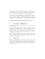
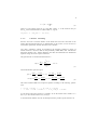
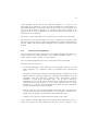
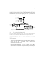
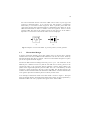
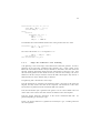
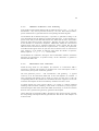
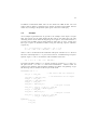
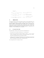
Published in
Analog and mixed signal description languages,
Current Issues in Electronic Modeling 10, chapter 6, 103-130, 1997
which should be used for any reference to this work
1
BEHAVIOURAL MODELLING OF
ANALOGUE SYSTEMS
WITH ABSYNTH
Vincent Moser, Hans Peter Amann, Fausto Pellandini
Institute of Microtechnology, University of Neuchâtel
Rue A.-L. Breguet 2, CH-2000 Neuchâtel, Switzerland
E-mail [email protected]
ABSTRACT
In this paper, we present the computer-aided analogue behavioural modelling tool
ABSynth (Analogue Behavioural model Synthesizer). The behaviour to model i s
expressed graphically in the form of a Functional Diagram (FD) drawn as the
interconnection of Graphical Building Symbols (GBS), each of which stands for some
elementary analogue behaviour. The functional diagram describes the behaviour of the
system only, not its physical structure. The corresponding HDL-A™ code is then
generated automatically.
The novel contribution of this work is threefold: first, analogue behaviour can be
described in a dedicated graphical form, secondly, the graphical description is translated
into behavioural AHDL code, lastly, the graphical description method and the code
generation process have been implemented as a software tool. This tool, ABSynth, i s
user-friendly, easy to extend, and integrated in a complete design environment. The
generated code is syntactically right by construction and, consequently, the user does not
need to know the syntax of the target hardware description language anymore.
1.
INTRODUCTION
Traditionally, analogue component modelling was reserved to experts who developed
very precise models of devices, particularly transistors. The models were written i n
general-purpose computer languages (e.g., C) and linked to the simulator. Nowadays,
the promoters of Analogue Hardware Description Languages (AHDLs) intend to make
modelling more popular among designers and must therefore make it a less specialized
2
task. However, the most important point remains unchanged: a good understanding of
the system or device to model is essential to write a good model. The coding technique
comes next but for all that it is not a trivial task. Therefore, we believe that some CAD
assistance must be provided to the designers who want to write their own models.
In this paper, we first introduce some definitions on analogue modelling followed by a
brief description of our coding method. Then a graphical description of analogue
behaviour is proposed, followed by a code generation strategy. These two points have
been integrated into the computer-aided modelling tool ABSynth (Analogue Behavioural
model Synthesizer). Some results will be given too, based on the example of an analogue
filter.
The whole work described here has already been the subject of a Ph.D. thesis [1]. Some
related work has also been the subject of conference papers [2], [3] and [4].
2.
ANALOGUE MODELLING
This section introduces general concepts and definitions of analogue modelling and our
model coding method.
A model of an analogue system can be represented either as a list of nodes and a list of
instances – both lists constituting a netlist – to describe its structure or as a list of
equations and/or other statements to describe its behaviour. A structural description can
be hierarchical, each instance of a netlist being also described as a netlist, but, as the
decomposition cannot be infinite, it always ends up with instances which are considered
at the behavioural level. This hierarchical structure can be seen as a tree, where the
behavioural instances are the leaves.
Beside the structural or behavioural internal description, a model also has an external
view, which describes its interface. It comprises pins and parameters. The pins are used
to instantiate the component in a structural description. The parameters are used to set up
the model to a particular application.
2.1.
Modelling Levels
In addition to different description styles (structural, behavioural), a system under
development can be described at various levels of abstraction. This can be represented i n
the Y-chart of figure 1, the analogue equivalent to the digital Y-chart of Gajski [5]. The
system can be described along three axes, each of which stands for a different view. The
abstraction level is indicated on each axis starting from the centre where the abstraction
is at its lowest.
ter
f.
ces
mo
del
s
dev
i
ces
dev
i
&
ou
rce
s
al s
e in
e in
ns
e
fac
ter
ns
ide
iv
vat
ser
con
iv
vat
ser
con
vio
ura
l
behavioural
view
n-
on
al
o
s, n
,
ms
beh
a
o
alg
rith
atio
equ
atio
equ
fun
ct i
,
eqs
o
alg
c
isti
er
act
device level
modelling
al
ide
r
cha
structural
view
,
eqs
mo
del
s
3
device layout
void
behavioural
modelling
macromodelling
cells
chip, MCM, µ-system
physical
functional
modelling
view
Fig. 1: Y-chart applied to analogue modelling.
As pointed out previously, a description of a system comprises a structural part and
behavioural descriptions of the component instantiated. On the structural axis we
indicate the type of component used while on the behavioural axis we indicate how the
component’s model is described. On the physical axis, the corresponding physical cells
are given. If we now consider the concentric circles, we can define several modelling
levels, each of which will be described in more detail below, starting from the origin of
the axes. In the area of digital design, the definition of 6 abstraction levels is widely
accepted. In the analogue area, however, these modelling levels are defined more
arbitrarily. Intermediate levels could also be defined. Furthermore, a system is usually
described in a mixed-level manner, where a combination of the modelling levels is used.
Also, note that the notion of abstraction level is related to the structure – the more
detailed the structure, the less abstract the description. It is not always linked to the
accuracy of the description, which depends on the level of detail of the associated
behavioural descriptions.
Device Level Modelling, also called primitive level, is the least abstract description. The
user describes the system structurally using standard devices (e.g., transistors,
capacitors, resistors), whose behavioural models are included in the simulator code.
These models are made of rather detailed characteristic equations of the devices whereas
second-order effects are also taken into account. Various models can be used depending
on the mode of operation of the device or on the degree of accuracy or simulation speed
4
needed. In the structural description, the connection points are electrical – or other
physical – nodes. They are described by Kirchhoff’s Current Law (KCL) and Kirchhoff’s
Voltage Law (KVL).
Macromodelling makes use of models of ideal components (e.g., resistors, capacitors,
inductors, independent and dependent sources) to build a circuit which mimics the
behaviour of the system instead of describing its actual structure [6]. Again, the
connection points are electrical nodes. Macromodels can be described in the SPICE
language or as particular circuit diagrams.
At the Behavioural Modelling level, the user builds behavioural models in an HDL using
differential equations, algorithmic sequences of statements or even tables of values. Any
analogue, mixed-signal or even non-electrical behaviour can be described. The
connection points of such models represent physical continuous-time signals, which are
not limited to electrical ones but can be of any nature. They are governed by generalized
conservation laws. For this reason, some typical behaviour like input impedance, output
impedance and power supply can be included in the behavioural models. The parameters
of the models are either given by the user to express specifications or are extracted from
existing circuits by lower level simulation or by measurement.
Once the user has become familiar with the HDL, this method becomes very efficient
since it is theoretically possible to describe any dynamic system. Furthermore, the
modelling level of detail can vary from idealized models to very accurate ones. However,
the current simulators are not optimized for behavioural simulation and can encounter
convergence problems, especially in the presence of discontinuities.
Functional Modelling, the most abstract modelling level, is used to describe complex
systems with little accuracy. Again, the models are described using an HDL and are
connected together in order to form a block diagram. The connection points are not
conservative but rather indicate a transfer of information as in a signal-flow model. This
can be realized either using a dimensionless variable (sometimes called a coupling) or
using either the across or the through quantity of a physical interface. As they are not
conservative, functional models must be handled carefully when they are integrated into a
mixed-level description.
2.2.
Analogue Model Generation Tools
Currently, several analogue modelling tools are available but most of them cover only
the structural part of a system’s description. The user places and connects symbols of
components using a graphical editor, then the netlist is automatically extracted. The
behavioural models of the components are either available in the libraries or they must
be “hand-typed” by the user.
The behavioural modelling part, however, has not been extensively automated yet. Some
interesting tools have been developed to generate behavioural models of s-domain and z-
5
domain transfer functions. The tools modgens and modgenz [7] convert transfer
functions into state-space representations in the time-domain and generate the
corresponding behavioural models in C. Similarly, gensims and gensimz [8] generate
ABCDL behavioural models starting from transfer functions. ABCDL (Analogue
Behaviour Circuit Description Language) is an HDL by AT&T Bell Laboratories.
In order to let the designers benefit from all the modern modelling possibilities,
graphical-based analogue behavioural model generation tools would be welcome,
especially such tools which allow the user to describe some arbitrary behaviour. The
models should be coded in a standard hardware description language in order to get
portable models which give the same simulation results on various simulators.
Furthermore, the models generated should be as compact and optimized as user-written
ones.
As we will see, the model generator ABSynth (Analogue Behavioural model Generator)
developed in this project fulfils most of these requirements.
2.3.
HDL-A in Short
ABSynth has been implemented to generate HDL-A code, a purely behavioural language
by ANACAD. The structural description must be expressed by means of SPICE-like
netlists. However, HDL-A is a mixed analogue-digital HDL since it includes a relation
block for analogue descriptions and a process block for digital descriptions. The process
block is a sub-set of the behavioural modelling facility of VHDL. We briefly describe
here some HDL-A concepts and constructs in order to allow the user to understand the
HDL-A examples given in this text. A more complete description of HDL-A can be found
in the User’s Manual [9]. As we are only interested in analogue modelling, we do not
discuss the digital part of HDL-A here.
An HDL-A model is composed of two parts: an entity declaration and an architecture
body. The entity gives an external view of the model and is associated to various
architecture to describe several internal views – i.e., implementations, behavioural
models, etc. – of the design.
The entity declaration gives the name of the design and the various connection objects
which compose its interface:
•
Generics are the parameters used to set up a model to a particular application.
•
Pins are analogue connection points. A pin has an associated nature property which
indicates the nature of the through and across quantities it carries. As pins carry two
quantities at a time, specific constructs are necessary to access each of them. For
example inp.i designate the current which flows through pin inp and inp.v
designate the voltage on pin inp.
6
The architecture body is composed of three different parts. In the first one – the
declaration block – all the analogue and digital variables are declared. The second o n e –
the optional relation block – is used to describe analogue behaviour. The third o n e –
the optional process block – is used to describe digital behaviour. HDL-A does not
include any structural coding facility. We describe below two analogue objects which are
important here:
•
A state – also called state variable – is an analogue object. It can be written in the
analogue part of the model (relation block) only but its value can be accessed in the
analogue part and in the digital part (process block). As a state has a history, it i s
possible to access its past values as well as its first time derivative and time integral.
•
A variable is a neutral object which can be written and accessed in the digital part and
in the analogue part. It is commonly used to store intermediate results or quantities
which do not need to have a history.
Analogue behaviour is coded in a relation block which begins with an initialization part
followed by explicit and implicit blocks, each of which is valid for one or more analysis
domains – i.e., DC, AC or transient analysis.
An explicit block – also called procedural block – is a sequence of analogue statements
which can be simple assignment statements, if-then-else constructs or iterative loops.
Expression can be formed using mathematical operators or predefined functions. When a
characteristic equation of a model can be coded as a direct assignment, it is called an
explicit equation and it can be coded in the explicit block. The operator which
symbolizes a direct assignment is :=. An additional assignment operator (%=) has been
defined to symbolize a contribution to a pin quantity.
An implicit block – also called equation block – is a set of characteristic equations
coded with yet another equality operator (==) which just indicates that the left-hand side
of the equation is equal to the right-hand side.
2.4.
Coding Method
The modelling method we propose here could theoretically be implemented in any
analogue hardware description language. Even if the terminology and the lexical
definitions vary from one language to another, the principles remain. Basically, we try
to split the behaviour to model into elementary behavioural elements, which are coded
separately and then combined. We show here solutions for some of these elementary
elements.
7
2.4.1.
Model Interface
In the modelling style we have established, the interface of a model is composed of
physical connection points (HDL-A pin) and of parameters (HDL-A generic). The pins
serve as connections between models when they are instantiated in the structural
description of a circuit. A pin carries a physical quantity represented as a couple of an
across variable (e.g., voltage) and a through variable (e.g., current). The parameters
allow the user to set up a model to a particular application.
In an analogue circuit, we can define a direction of propagation of the information
through a chain of signal processing elements. The physical quantities that carry this
information, however, are directionless. Each model is influenced by the across
quantities on all the nodes to which it is connected and by the through quantities on all
its pins. Reciprocally, each node is influenced by all the components connected to it.
Consequently, a model can read the value of the across and of the through quantity on any
pin but it can also impose its own contributions to these values. The final value of the
across and through quantities are then computed at simulation time according to the
contributions of all the components.
In practice, the four read/contribute possibilities are rarely used simultaneously.
According to our experience, most of the models can be realized with a restrictive pin
usage: the model uses the value of the across quantity on all the surrounding nodes t o
calculate the value of the through quantity on each pin. Theoretically, the dual way –
i.e., read the through quantity and calculate the across quantity – can also be followed
but it seems that some simulators hardly accept it.
As another convention, we attribute a positive sign to any through quantity that enters
the model. According to this choice, we can define a complete model interface which does
not only include pins but also builds a complete input stage, a complete output stage or a
power supply block.
Some pins can be considered as passive accesses where either the across or the through
value is read and the dual value is imposed. Note that the value imposed may be the result
of complex non-linear computations. Functionally, this access can be seen as an input
stage. If this input stage is modelled as a resistance Rin and a capacitance Cin connected i n
parallel, we have the following equation
iin = Cin
dVin
+ Vin Rin ,
dt
(1)
which gives the following HDL-A code:
IN_PIN.i %= Cin*ddt(IN_PIN.v) + IN_PIN.v/Rin
Some other pins can be considered as non-ideal sources with an internal impedance. This
source-type behaviour characterizes an output stage governed by the equation
8
iout = (Vout − V0 ) Rout
(2)
where V out is the voltage on the pin, V 0 is the ideal voltage, iout is the current on the pin
and Rout is the internal resistance. Coded in HDL-A, it gives:
OUT_PIN.i %= (OUT_PIN.v - v0)/Rout;
2.4.2.
S - domain
Modelling
We have seen how to code the interface of the model. We now look at the heart of the
model, where the desired behaviour is implemented. In this section, we will see how t o
code models specified by transfer functions in the s-domain.
Very often, continuous systems are specified in the frequency domain by means of
transfer functions. However, HDL-A, and presumably VHDL-AMS, offer time-domain
description facilities only. Transfer functions must then be transformed into differential
equations using the inverse Laplace transform.
The general form of a rational transfer function is
M
Y (s)
H (s) =
=
X (s)
∑a
m
sm
m=0
N
1 + ∑ bn s n
, M≤N
n =1
(3)
which time-domain equivalent gives
dy(t )
d 2 y(t )
d N −1 y(t )
d N y(t )
+ b2
+
…
+
+
b
b
N −1
N
dt
dt 2
dt N −1
dt N
M −1
2
dx(t )
d x (t )
d x (t )
d M x (t )
= a 0 x ( t ) + a1
+ a2
+ … + a M −1
+ aM
M −1
2
dt
dt
dt
dt M .
y(t ) + b1
(4)
This can be coded in HDL-A as an implicit equation according to the following pseudocode.
y + b1*dy + b2*d2y + ... + bn_1*dn_1y + bn*dny
== a0*x + a1*dx + a2*d2x + ... + am_1*dm_1x + am*dmx;
As only the first derivative operator is available, we use the internal state variables dmx
and dny to store the derivatives of x(t) and y(t).
A rational transfer function can also be decomposed into a product of poles and zeros as
9
M
H (s) = H0
∏ (s − ζ )
m
m =1
N
∏ (s − p )
, M≤N
n
n =1
(5)
where ζm are the coordinates of the zeros and pn the coordinates of the poles. Each
member of those products can be modelled separately and the whole system is built b y
cascading all the sub-systems. For each type of sub-system, we give HDL-A solutions as
particular forms of the general differential equation coded above.
Single real pole located at coordinates p in the s-plane
x + 1.0/p*dy - y == 0.0;
Pair of complex conjugate poles p, p* at α p±jβp
x - 1.0/(ap*ap+bp*bp)*d2y + 2.0*ap/(ap*ap+bp*bp)*dy - y == 0.0;
Single real zero at ζ
y := x - 1.0/z*dx;
Pair of complex conjugate zeros ζ, ζ* at αz±jβz
y := x - 2.0*az/(az*az+bz*bz)*dx + 1.0/(az*az+bz*bz)*d2x;
Besides poles and zeros, other building blocks, like limitations or delays, can also be
defined. Additionally, it is possible to model sample-data behaviour using an AHDL, as
described in [4].
3.
GRAPHICAL DESCRIPTION
Modelling with an Analogue Hardware Description Language requires a very good
knowledge of the language syntax. As such, this task is unfortunately reserved t o
specialists. If we want to promote analogue behavioural modelling among designers,
computer-aided design tools with convenient user interfaces must be provided. Ideally,
such tools should be integrated in the design environment that is already used for circuit
design. VHDL and Verilog have been accepted and used successfully by the digital design
community when computer-aided modelling tools have been available, although
automatic logic synthesis tools have played a decisive role in this too. Furthermore, i t
has been shown that the overall design productivity is improved by the use of graphical
HDL-based design tools [10].
In the previous section, we presented a behavioural modelling method. Here, we propose
to formalize this knowledge in a graphical form. This representation can be seen as a
10
first step towards an automatic code generation process, which will be exposed in the
next section. It has been designed to remain of general use and independent of any
particular hardware description language.
3.1.
Specifications of the Graphical Description Set
In order to model dynamic systems accurately, a graphical description set must include
the following features:
•
Description of the structure of a system as the interconnection of components
through a physical – i.e., across-through – interface.
•
Description of the behaviour of a system or component, using non-physical
variables for the information propagation and processing.
•
Description of generic models including a set of parameters.
•
Aptitude to an implementation as a front-end to a computer program.
3.2.
Existing Graphical Description Methods
Before designing a new graphical description set, we review several existing graphical
modelling techniques, each of which is discussed and compared with our specifications.
More information on these description techniques can be found in [11].
Circuit diagram modelling is well-known; it has been widely used by electrical and
electronic engineers for years. The basic components of electrical engineering (i.e.,
resistors, transistors, sources, etc.) are available as symbols, each of which is composed
of a body, pins and a set of parameters. These basic components are linked to an implicit
model, which can be as simple as Ohm’s law for a resistor or as complex as a full equation
set to describe a MOS transistor. The connection points between the instances are
defined as electrical nodes, implicitly described by KCL and KVL.
Circuit diagram modelling is basically a structural technique. The behaviour of the circuit
is given by the diagram structure and by the implicit models of all the components. To
analyse a whole circuit, we must list the characteristic equations of all the components
involved and list the equations that correspond to KCL on each node and KVL on each
mesh.
This representation has also been used to describe the behaviour of systems in a
macromodelling approach, but the limitations of this technique, as shown previously,
remain.
11
As explained above, the nets of a circuit diagram represent both the across and the
through quantities and there are neither input nor output ports. For this reason, it is not
suitable for the description of signal propagation or signal processing elements and,
consequently, circuit diagram modelling cannot be applied to the behavioural description
of analogue systems.
Block diagrams have been widely used by engineers in many different application
domains. Blocks, which have input and output ports are connected by oriented paths. A
path represents a signal, which can be either an across or a through quantity or even an
abstract variable. A block represents a transducer which functionality is indicated either
graphically or with an equation. A take-off point is introduced in order to bring the
signal to both blocks.
As nearly any block can be defined, block diagrams can be used to describe linear as well
as non-linear systems. As the across and through variables appear separately in the
block diagram, it can neither represent the structure of a physical system – i.e., an
electrical circuit – nor describe any physical interface. The behaviour of a system,
however, can be represented conveniently.
The Signal-Flow Graph (SFG) representation is very similar to the block diagram. A
signal, instead of being represented by a path, is now represented as a node, which can be
used directly as a summer node or as a take-off point, whilst a path now represents a
transducer. A SFG is limited to the description of linear systems. This description
technique can also represent a behaviour but it is less intuitive than block diagrams.
However, as the number of graphical element is reduced (path and nodes), it can be more
easily implemented as a front-end to a computer program.
Another graphical description method is the bond graph. A bond is represented as an
harpoon, which carries both through and across variables. The bonds are connected
together using two types of junctions. In a 0-junction, all across variables are equal and
all through variables add up to zero: it is a generalization of KCL. In contrast, in a 1junction, all through variables are equal and all across variables add up to zero: it is a
generalization of KVL. This method is not very intuitive for the novice user, but it i s
very powerful for the structural description of physical systems. However, it is not well
suited to behavioural descriptions where non-physical variables are used instead of
across-through couples.
3.3.
Analogue Behavioural Description Method
None of the description techniques discussed in the previous section fully satisfies all the
requirements. The main problem is to find a method which supports both a structural
description using across and through variables and a behavioural signal processing
description using abstract variables. For this reason, different methods are used for
different purposes.
12
Circuit diagrams will be used for the structural description of a system as the
interconnection of components. As this classical representation is already available i n
most design frameworks, it will be left aside in the rest of this text. The emphasis will
now be on the behavioural description of components and systems. However, the
physical interface of the components must also be described to allow them to be
instantiated in circuit diagrams.
The interface will be represented as an icon, which gives an external view of the model.
The behaviour will be described using a new type of extended block diagram called
functional diagram (FD) which is built using standard blocks called Graphical Building
Symbols (GBS). This new description technique will be explained in the following
sections.
3.4.
The Icon of a Component
The icon is the graphical object that can be used to instantiate the behavioural model in a
circuit description. It is then equivalent to any standard component symbol – i.e.,
resistor symbol, transistor symbol, etc. More formally:
The icon describes graphically the interface of the model with its environment.
Practically, the icon consists of:
•
A body which should give a first visual idea of the component’s function. For some
usual components (e.g., comparators, filters), conventional body representations
exist.
•
Pins used to interconnect the component with other elements in a higher level circuit
diagram. Basically, an analogue component is influenced by the quantities on all the
surrounding nodes and reciprocally influences them. Consequently, analogue
quantities – of both across and through type – can be read or written as
contributions to pins. For this reason, the pins have to be defined as bi-directional.
Furthermore, they can be electrical or of any other physical nature (i.e., fluid,
mechanical, etc.). The pins form the interface of the model with other components
placed in the same circuit or system description.
•
Optional properties, which are the parameters of the model. They allow the user t o
set up a generic model for a particular application. Each property is defined with a
default value. The properties are the interface of the model with the user.
•
Optional textual comments to better describe the function of the model.
As an example, we model a fifth order elliptic low-pass filter as described in [12]. A
model icon (figure 2) has been defined with four pins and ten properties – the
13
coordinates of the poles and zeros of the transfer function, the input capacitance, the
output resistance and the value of the static supply current.
Fig. 2: Icon of a fifth order elliptic low-pass continuous-time filter.
3.5.
The Functional Diagram
The functional diagram is a schematic representation of an analogue behaviour given i n
the form of an extended block diagram. Some graphical building symbols, which stand
for elements of behaviour are put together and interconnected in order to describe a more
complex behaviour. Expressed more formally:
The Functional Diagram (FD), built as an assembly of interconnected Graphical Building
Symbols (GBSs), describes the behaviour of the model.
Note: The structure of the FD does not match the structure of any particular physical (e.g.,
electronic) realization of the component. Only the behaviour is described.
The functional diagram contains the semantics of the model. This semantics i s
determined firstly by the interconnection scheme of the GBSs in the diagram and
secondly by the semantics of each GBS.
The functional diagram is drawn with a graphical editor, that allows GBSs to be chosen
from a library, placed in a schematic and connected by wires. As in the block diagram
formalism, a wire represents a one-dimensional, non-physical, continuous-time state
variable. Connection points on a GBS are oriented and thus indicate the direction of
propagation of the information throughout the model. The following connection rule
applies: the output pin of a GBS can be connected to an unlimited number of input pins
but cannot be connected to another output pin (conflict).
Once the internal behaviour has been described, bi-directional pins, which correspond t o
the pins on the model’s icon, are placed around the diagram. Particular GBSs are added t o
compose the interface between the physical quantities on the pins and the internal
variables of the model.
14
In order to obtain the desired behaviour, the user can adjust the properties of some GBSs.
The value attributed to the properties can be either numerical or it can be an expression i n
which the external parameters of the model – as defined on the icon – appear.
If we now go back to our continuous-time filter, we can draw a functional diagram
(figure 3) to describe its behaviour.
Fig. 3: Functional diagram of a fifth order elliptic low-pass continuous-time filter.
We can first recognize an RC-parallel input stage. The value of the voltage on the input
pin is read using a voltage probe GBS. This way the physical across quantity voltage i s
translated into an abstract variable. This value is multiplied by the constant which
represents the input conductance using a gain GBS. In a parallel path, its derivative i s
multiplied by the input capacitance cin – a parameter of the model. The sum of these two
terms is written as a current contribution to the input pin by means of a current generator
GBS. Now, the abstract variable is translated into a physical through quantity of type
current. Then, the transfer function is modelled as a series of GBSs, which represent a
single pole (pole1 GBS), two pairs of poles (pole2 GBS) and two pairs of zeros (zero2
GBS) respectively. Again, the parameters of the model – icon properties – appear o n
the various GBSs.
The output of the transfer function could be used directly as the ideal output voltage value.
Here, we rather feed it to a resistive output stage in order to model a non-ideal output. The
ideal value is compared to the actual value of the voltage on the output pin and divided b y
the output resistance rout. The resulting value is imposed as a current contribution to the
output pin.
Finally, a power supply with static supply current isupstat has also been defined. The
positive and negative current terms are split up using separator GBSs and imposed as
current contributions to VSS and VDD respectively.
15
If a component must be modelled differently depending on the analysis type (DC, AC,
transient), the behaviour can be described in several analysis-specific functional
diagrams. This facility will usually be referred to as multi-FD modelling. Figure 4 shows
a functional diagram of our low-pass filter valid only in DC mode. All the derivatives are
removed from the original FD. The new input stage is now purely resistive and the
transfer function is replaced by a wire.
Fig. 4: DC-mode FD of a fifth order elliptic low-pass continuous-time filter.
3.6.
The Graphical Building Symbols
The graphical building symbols are spare parts which represent elements of behaviour
and which are used to build a more complex behavioural description. In other words:
A Graphical Building Symbol (GBS) is the graphical representation of an analogue
function.
A GBS is composed of:
•
A graphical body drawn so that it gives a good idea of the corresponding behaviour.
The body and the name of the GBS together represent the semantics of the GBS in a
graphical way. If the body is not meaningful enough, an additional textual
description must be provided to the user.
•
Optional input and/or output pins. In a functional diagram, the information i s
transformed in the GBS and transits in the form of a variable from one GBS t o
another through pins. Therefore, they must be oriented. Input pins are bound to the
symbol with an incoming arrow so that they can be visually identified. Any pin
16
which is on the physical side of a read/write conversion GBS, however, must be
declared bi-directional and marked with a bi-directional arrow. Each pin must also
have a distinct name.
•
Optional properties, which allow the user to adjust a GBS instance to a particular
need. For example, the gain GBS has a property, also called gain, which can be set t o
an arbitrary value to determine the multiplying factor between the input and the
output.
The range of behaviour that can be represented by a GBS varies from elementary
mathematical operators to arbitrarily complex sets of equations. However, a set of basic
GBSs is defined, which can be classified in the following categories:
•
Operator GBSs: they mainly represent current mathematical operators. Beside the
four basic operators, time differentiation and integration are defined as well as gain,
sign, poles, zeros and some others. Figure 5a shows an 2-input adder GBS
characterized by
OUT = IN1 + IN 2
(6)
where IN1 and IN2 are the two input pins of the GBS and OUT is the output pin.
Figure 5b shows a gain GBS characterized by
OUT = gain ⋅ IN
(7)
where IN is the input pin of the GBS, OUT is the output pin and gain is a property of
the GBS.
a)
b)
Fig. 5: Examples of operator GBSs: a) 2-input adder b) gain.
•
Function generation GBSs: functions like sine or cosine can be generated to be used
in the model. Figure 6 shows a sine GBS characterized by
OUT = sin( IN )
(8)
17
where IN is the input pin of the GBS and OUT is the output pin. In this equation IN
carries the argument of the sine function.
Fig. 6: Example of function generation GBS: sine function.
•
Parameter GBSs: most of the model parameters (icon’s properties) correspond, in the
functional diagram, to properties of GBS instances – e.g., the property gain of a
gain GBS. However some free parameters must also be available directly in the FD.
For this reason an additional parameter GBS has been defined. It has one property –
the actual parameter – and one output pin which carries the value of the parameter.
Additionally, some GBSs access simulation parameters like time or model
temperature. Figure 7a shows a free parameter GBS characterized by
OUT = parameter
(9)
and figure 7b shows a temperature GBS characterized by
OUT = temperature
a)
(10)
b)
Fig. 7: Examples of parameter GBSs: a) free parameter b) model temperature.
•
Conversion GBSs: inside the FD, the wires which connect the GBSs are oriented and
they represent non-physical variables only. When the model is used in a circuit
diagram, however, its pins are connected to physical nodes. As explained above,
these pins are not oriented and they carry a pair of quantities – an across quantity and
a through quantity. Some conversion elements are then necessary to interface the two
description modes. In the FD, the pins of the model, which are represented b y
particular connector symbols to indicate the boundary of the FD, can exclusively be
connected to a particular class of GBSs, called conversion GBSs. These are used t o
access the physical quantities on the pins and translate them into variables, a form
18
that can be used inside the FD. Conversion GBSs can be either of probe type and
represent a read functionality, or of generator type and represent a contribution
functionality or even both at a time. Figure 8a shows a pressure probe GBS. The
value of the pressure read on the fluid input pin is transmitted to the output pin of the
GBS and can therefore be used as a variable in the FD. Figure 8b shows a current
generator GBS. The value of the variable present on the input pin of the GBS i s
imposed as a contribution to the current on the electrical output pin.
a)
b)
Fig. 8: Examples of conversion GBSs: a) pressure probe b) current generator.
3.7.
Hierarchical Design
In practice, functional diagrams can be quite complex and it is obvious that a diagram
with more than a few tens of GBSs becomes difficult to read. For this reason, hierarchy
has been introduced. The idea is as follows: a new hierarchical GBS is designed to replace
part of the original functional diagram.
First the new GBS is drawn according to the rules given in § 3.6. The orientation of the
different pins is defined in such a way that the new GBS can be directly placed in the
original FD. Then, a sub- functional diagram (sub-FD) is drawn, which contains the
portion of the original FD replaced by the new GBS. This core is surrounded by oriented
connectors, which correspond to the pins of the new GBS. The sub-FD expresses the
semantics of the hierarchical GBS. The hierarchical GBS and the associated sub-FD form
a new generic object that can then be placed in a library for later reuse.
As an example, a hierarchical variant of our filter model is shown in figure 9. The input
stage, the transfer function, the output stage and the power supply are now represented b y
hierarchical GBSs. The icon’s properties also appear on the various GBSs.
19
Fig. 9: Hierarchical FD of a fifth order elliptic low-pass continuous-time filter.
If we look in more detail at the output stage (figure 10), the property R is defined on the
hierarchical GBS and it appears in the expression of the gain property of a gain GBS
inside the sub-FD. The sub-FD also includes conversion GBSs (a current generator and a
voltage probe). For this reason, the hierarchical GBS is considered as a conversion GBS
with read/write functionality and the corresponding pin is defined bi-directional. The
other pins are an input pin and an output pin which allows the user to access the variable
i out .
Fig. 10: Hierarchical GBS and sub-FD of a resistive output stage.
A sub-FD can contain other hierarchical GBSs without limitations on the number of
hierarchy levels. However, recursive description – i.e., the use of a hierarchical GBS i n
the sub-FD associated with itself – is not allowed.
It is also possible to combine multi-FD description with hierarchical modelling. In this
case, the component is described by three different analysis-specific functional
diagrams, each of which contains hierarchical GBSs. Furthermore, one can define a
hierarchical GBS associated with three analysis-specific sub-FDs.
20
4.
AUTOMATIC CODE GENERATION
The modelling experience gathered in this project has led to the development of a
graphical method for the description of analogue behaviour. In a second step towards
computer-aided modelling, the equivalent hardware description language model code will
be generated starting from this graphical description. The whole process will be
considered as successful if the resulting HDL model can be compiled without syntax
errors and simulated. Obviously, the simulation results must also match the
specifications.
First the specifications of the code generator are given. Then, an entity generator and an
architecture generator will be described in detail. These two code generators constitute
the core of the program ABSynth.
The general objectives of the code generation tool are:
•
The code generator to develop must automatically translate the semantics of an
analogue model given graphically as an icon and a functional diagram into an HDL
file.
•
The generated code must contain the complete description of the model and it must be
syntactically right by construction.
•
After compilation of the generated code, it must be possible to instantiate the model
in a circuit description for simulation.
•
The generated models should be coded in a standard HDL.
The hardware description language we choose for the long term is VHDL-AMS – the IEEE
mixed-mode extension of VHDL [13]. As VHDL-AMS has not been completely defined
and approved yet (Dec. 1996), our automatic code generator must be developed for a
proprietary modelling language of the VHDL family. Consequently, it must be designed
so that it can be easily updated to the standard language. For this reason, the code
generation approach must be as independent as possible of a particular language syntax.
It is obvious, however, that the definitions of the target HDL syntax must be included i n
one form or another in the program.
In order to determine the level of language independence we want to achieve, we make the
difference between some general language constructs that are common to all the VHDLlike languages and some more specialized language constructs – i.e., keywords, standard
functions, etc. The information relative to the general language structure can be part of
the code generation program. The more specialized definitions, however, should be
stored out of the main program so that they can be updated easily.
21
We assume that VHDL-AMS models will have the same entity-architecture structure as
VHDL models. Furthermore, some entities can have several associated architectures.
Consequently, we split up the code generation task into two parts:
•
An entity generator, which translates the information relative to the icon into an
entity declaration. This generator is described in more details below.
•
An architecture generator, which translates the semantics of a functional diagram
into an architecture description. Two strategies can be defined to generate the
architecture part. It can be either a behavioural description made of a collection of
statements or a structural description based on signal-flow semantics. The
behavioural architecture generator is described in detail below.
To be considered right by construction, the generated models must strictly follow the
target language syntax, but we can limit our approach to a sub-set of the language. Here,
we implemented a sub-set of ANACAD’s HDL-A which seems compatible with the spirit
of VHDL-AMS. For instance, we only generate purely analogue models since the digital
VHDL part is already covered by other tools. Some other limitations will be indicated
along this chapter.
4.1.
Entity Generator
An HDL-A entity clause describes the interface of a model, which, in our graphical
description, corresponds to the icon. The entity must have a name and can have several
connection points and parameters. The following correspondences have been defined:
•
The name of the entity is the same as the name of the graphical component.
•
Each bi-directional pin of the icon is expressed as an analogue pin declaration of the
same nature.
•
Each property of the icon is expressed as a generic declaration with its default
value.
We now describe the entity generation process that translates the icon description into
the HDL-A entity clause. First, the information is read from the graphical database. The
model name, the property names and the corresponding default values are stored i n
memory. The default values cannot be used in the HDL-A entity declaration, but this will
be possible in VHDL-AMS. The pin names are stored too, together with the
corresponding values of the property nature. If no nature property is found, the pins are
assumed to be electrical.
In a second step, the actual entity declaration code is written in a file. The first line of
code is built according to the syntax and using the name of the model as stored
previously. Then, if generics are present, the generic clause is written. For each generic,
22
a generic_list line is written. In fact, there is only one generic identifier per line. A
sample generic_list code line is copied from a template file, the word generic i s
replaced by the actual generic name and the resulting customized line is copied to the
output file.
The generic template line is:
generic : real
Then, the pin declarations are issued in a similar way. The difference is that both the pin
name and the nature attribute must be set according to the pin description. The actual pin
name takes the place of the word pin, while the value of the optional property nature
replaces the word electrical in the following template:
pin : electrical
Once the generic and pin declarations are complete, the remainder of the entity
declaration clause is written.
As an illustration, we go back to our filter example. The model name is ellip5, the icon
has ten properties – sigma0, 1 and 3, omega1 to 4, cin, rout and isupstat – and
four electrical pins – SIG_IN, VDD, VSS and SIG_OUT. The properties are expressed as
real generic declarations
ENTITY ellip5 IS
GENERIC (
sigma0 : real;
sigma1 : real;
omega1 : real;
omega2 : real;
sigma3 : real
omega3 : real;
omega4 : real;
cin : real;
rout : real;
isupstat : real
);
and the electrical pin declarations are added.
PIN (
SIG_IN : electrical;
SIG_OUT : electrical;
VDD : electrical;
VSS : electrical
);
END ENTITY ellip5;
23
4.2.
Behavioural Architecture Generator
In addition to the entity generator, an architecture generator has been developed. The
semantics of the functional diagram is translated into an architecture body using
behavioural statements. The semantics of the GBSs is given in code templates that are
written in the target language syntax and stored in a library. First, we give some general
information on the architecture generation process. Then, the different parts of the
architecture generator are described.
4.2.1.
Generalities
In order to link the graphical model description and the code to generate, the following
correspondences have been established between the FD and the HDL-A architecture
block.
•
The name of the architecture is identical to the name of the FD.
•
A GBS instance is translated into a piece of HDL code.
•
A GBS property becomes a real variable, which must be initialized according to the
value of the property.
•
A GBS pin becomes an analogue state variable.
•
A net becomes a state variable assignment statement.
The basic idea behind the architecture generator is that each GBS is associated with a code
template written in the target syntax. Based on this information, the final code i s
generated in a two-step sequence:
(1) For each GBS instance, a copy of the corresponding code template is made and the
identifiers are modified according to the instance name in order to ensure their
uniqueness and the information that corresponds to the interconnections between the
GBSs is added to the code as simple assignment statements. This is called the code
customization process.
(2) All those customized code segments are gathered into a single code file. This is called
the gathering process.
4.2.2.
Code
Customization
As explained above, code customization is the first stage of our behavioural architecture
generator. This process transforms a generic code template related to a GBS into a
24
customized code segment according to the name and to the properties of a particular
instance of this GBS. It must fulfil three tasks:
•
In the generic code template, the identifiers are generic; in the final code, they must
be unique. To achieve this, the name of the GBS instance is used as a prefix to each
identifier.
•
In the generic code template, the properties of the GBS are initialized to a default
value; in the final code, they must be initialized to the value of the corresponding
property of the GBS instance. This value is changed accordingly in the initialization
part.
•
In an FD, each non-interface input of a GBS is connected to the output of another
GBS. This information is expressed in the model code as a new statement: the value
of the output state of the preceding GBS is assigned to the corresponding input
state.
For example (figure 11), the input pin in of a gain GBS instance I2 is connected to the
output pin out of the GBS instance I1. The value of the gain is set to 1000.
Fig. 11: GBS customization example.
The primitive code template of the gain GBS is
ARCHITECTURE imt_hdla OF gain IS
STATE in, out : analog;
VARIABLE gain : real;
BEGIN
RELATION
PROCEDURAL FOR init =>
in := 0.0;
out := 0.0;
gain := 1.0;
PROCEDURAL FOR dc, ac, transient =>
out := gain * in;
END RELATION;
END ARCHITECTURE imt_hdla;
The resulting code is as follows
25
ARCHITECTURE imt_hdla OF gain IS
STATE I2in, I2out : analog;
VARIABLE I2gain : real;
BEGIN
RELATION
PROCEDURAL FOR init =>
I2in := 0.0;
I2out := 0.0;
I2gain := 1000.0;
The identifiers have been modified and the value of the gain has been set to 1000.
PROCEDURAL FOR dc, ac, transient =>
I2in := I1out;
The value of the variable I1out is assigned to I2in.
I2out := I2gain * I2in;
END RELATION;
END ARCHITECTURE imt_hdla;
4.2.3.
Single FD Architecture Code Gathering
Code gathering is the second stage of the behavioural architecture generator. It aims at
gathering all the previously customized code segments into a single model. If the
behaviour of the model in the three analysis domains is described in the same functional
diagram, graphical information reading and code customization are done only once. Then
the code can be gathered for each block successively. Note that the resulting code can be
different in the three analysis domains because the GBS code templates may describe a
different behaviour in the different analysis domains.
The gathering task is divided into several steps.
First the declarations are generated. The architecture name is the name of the functional
diagram, the entity name is the name of the component. The declarations of the states
and variables are gathered from the customized GBS code segments.
Then, the initialization part is generated. The generics are set to their default value. The
initial values of the various states and variables are defined in the code templates.
Then, the explicit behaviour description of the various customized GBS code
gathered depending on the analysis type.
are
Finally, the implicit behaviour is gathered for each analysis type, including unknown
lists and equations.
26
4.2.4.
Multi-FD Architecture Code Gathering
If the graphical model includes different FDs for different analysis types – i.e., DC, AC
and transient – they will be processed successively. First, the three analysis-domainspecific architectures are generated from the corresponding functional diagrams.
An intermediate DC architecture description, if specified, is generated according to the
code customization and code gathering procedures described above. As the description i s
specific to DC analysis, the states and variables also differ from the states and variables
used in the other analysis-specific descriptions. Therefore, the string DC is prefixed t o
all the identifiers to ensure their uniqueness. Additionally, dummy AC and transient
equation blocks must also be generated. Indeed, the syntax requires that the same
unknowns must be declared in all the three equation blocks. To satisfy this requirement,
each unknown that appears in the DC part must also be declared in the AC and transient
parts. Moreover, as the number of unknowns must match the number of equations,
dummy equations – i.e., yy == 0.0; – must be added.
An intermediate AC architecture description and an intermediate transient architecture
description are generated too, if specified. Finally, all this information is gathered t o
form the final model code.
4.2.5.
Hierarchical Code Generation
Instead of being stored as a code template, the semantics of a hierarchical GBS i s
expressed as a sub-FD. This semantics is translated into a new code template so that i t
can be used by the top-level architecture generator.
The code generation process – code customization, code gathering – is applied
recursively to all the hierarchical GBSs until all the code templates are available. A
newly generated code template can be stored in a library for later reuse so that the
corresponding GBS can be considered as a flat GBS the next time it appears in an FD. The
associated code template can then be used directly and much CPU time is saved.
As already pointed out in the previous chapter, it is possible to combine multi-FD
modelling with hierarchical modelling. If the model is described by analysis-specific
functional diagrams that contain hierarchical GBSs, the hierarchy is solved first and then
the final code is generated using the newly generated code templates.
On the other hand, if a hierarchical GBS is described by three analysis-specific sub-FDs,
the corresponding code template must be generated first. Then the new code template can
be used as usual.
27
In addition to hierarchical GBSs, users can also define new GBSs of their own. The
symbol must be drawn as explained above and the associated code template must be
written too, according to the particular syntax given in the User’s Guide [14].
4.3.
Example
As an example of generated code, we go back to the example of the elliptic low-pass
filter. We will not give the whole model code here, but we will rather point out some
interesting extracts. In the functional diagram given in figure 4, the transfer function i s
given as a series of GBSs, each of which stands for either poles or zeros. A single pole
and a pair of poles are modelled in HDL-A using the following implicit equations,
respectively
in - (-1.0/(twopi*p)) * ddt(out) - out == 0.0;
in - b1 * dout - b2 * ddt(dout) - out == 0.0;
where b1 and b2 are functions of the coordinates of the poles and where dout is the first
derivative of the output state out. A pair of zeros, however, is modelled using an explicit
equation. Again, a1 and a2 are functions of the coordinates of the zeros.
out := in + a1 * din + a2 * ddt(din);
The single pole GBS is instance I706, the pair of poles are respectively I707 and I708,
the pairs of zeros I709 and I710. After code customization – instance names are
prefixed to the identifiers and assignment statements are added – and gathering we get
the following code, for instance for the AC part of the model:
PROCEDURAL FOR ac =>
-- GBS I706 to GBS I707 connection
I707_in := I706_OUT;
-- 1st derivative of I707 output
I707_dout := ddt(I707_out);
I708_in := I707_OUT;
I708_dout := ddt(I708_out);
I709_in := I708_OUT;
I709_din := ddt(I709_in);
-- 1st pair of zeros
I709_out := I709_in + I709_a1 * I709_din
+ I709_a2 * ddt(I709_din);
I710_in := I709_OUT;
I710_din := ddt(I710_in);
-- 2nd pair of zeros
I710_out := I710_in + I710_a1 * I710_din
+ I710_a2 * ddt(I710_din);
...
EQUATION (
I706_out,
I707_out,
28
I708_out
) FOR ac =>
-- single pole
I706_in - (-1.0/(twopi*I706_p)) * ddt(I706_out)
- I706_out == 0.0;
-- 1st pair of poles
I707_in - I707_b1 * I707_dout - I707_b2 * ddt(I707_dout)
- I707_out == 0.0;
-- 2nd pair of poles
I708_in - I708_b1 * I708_dout - I708_b2 * ddt(I708_dout)
- I708_out == 0.0;
5.
RESULTS
The graphical description and the code generation strategy have been implemented as the
tool ABSynth and integrated in the Mentor Graphics Falcon Framework. In order t o
benchmark ABSynth, we first measure the code generation time in various situations.
Then we compare two ABSynth models with an HDL-A model coded manually. Our
criterion will be code size, simulation results and simulation time. The benchmark
example used is the elliptic low-pass filter already treated in the previous sections. Code
generation time and simulation time are CPU time measured on a Sun Sparc 20/71
workstation – rated 126 SpecInt92 and 121 SpecFt92.
5.1.
Code generation time
We generate HDL-A models of the low-pass filter in three different ways:
•
Starting from the flat functional diagram given as explained above.
•
Starting from the hierarchical functional diagram of figure 9. In a first run the
generic code templates which correspond to the hierarchical GBSs are not available.
They must be generated and can be saved in the user library.
•
Starting once more from the hierarchical FD. In this second run, the previously
generated generic code templates of the hierarchical GBSs are taken from the user
library. The resulting code is the same as in the previous case.
The code generation time is displayed in table 1.
29
Model
Flat
Hierarchical
(1st run)
Hierarchical
(2nd run)
CPU time
45 s
49 s
16 s
Table 1: Code generation time.
We first see that code generation starting from a hierarchical description is somewhat
slower than from a flat description. However, when generic code templates of
hierarchical GBSs can be reused, the CPU time is reduced in an important manner – i n
this case by a factor of 3.
5.2.
Code size
Table 2 displays the size of the different models generated as well as the size of a
manually coded version of the same filter. We compare the number of code lines, the
number of states and the number of variables.
Model
Manual
Flat
Hierarchical
# Lines
103
453
467
# States
8
55
63
# Variables
15
22
33
Table 2: Model code size.
Obviously, automatically generated code is less compact than code written directly by a
modelling engineer. In this case, the biggest difference lies by the number of state
variables necessary. This is not surprising because ABSynth uses a state variable for the
output of a GBS and another one for the input of the GBS to which it is connected even if
they both carry the same information. However, the flat description and the hierarchical
description lead to code of the same complexity.
5.3.
Simulation results
The different models are then simulated and we obtain in all cases exactly the same
curves. The results of an AC simulation of the low-pass filter are displayed in figure 12.
30
Fig. 12: Simulation of a fifth order elliptic filter.
5.4.
Simulation time
Simulation time, however can vary greatly from one model to another. Table 3 shows
the simulation time needed by each model in the case of an AC simulation and in the case
of a transient simulation.
Model
Manual
Flat
Hierarchical
AC simulation time
10 s
16 s
16 s
Transient
simulation time
2.5 s
3.6 s
3.6 s
Table 3: Simulation time.
As the manually written model is much faster than the ones we generated with ABSynth,
the generated code should be optimized. A first idea is to reduce the number of state
variables and the number of lines of code. This could be done by modifying the code
customization process in such a way that the output of a GBS would be represented by the
same state variable as the input of the next GBS. This way one state variable and one
assignment statement could be saved for each inter-GBS connection. This point has not
been investigated further and it is left for future work.
31
6.
CONCLUSIONS
In this text, we searched for a way to support designers in modelling analogue systems.
The solution we propose is twofold. First, the users have to graphically describe the
behaviour of the system they want to model. Second, this graphical description i s
translated into an analogue hardware description language.
6.1.
Main Contributions
A first contribution of this research is a method for the graphical description of analogue
behaviour. We introduce the functional diagram, an extended block diagram, which
allows the users to build complex behavioural descriptions using behavioural building
blocks called graphical building symbols. The users can clearly define the boundary
between the internal behavioural description based on signal flow variable processing
and the external interface of the system based on the exchange of physical quantities.
A second contribution is a code generation strategy developed to translate the semantics
of a functional diagram into behavioural HDL code. This strategy includes the handling
of hierarchical and analysis-specific functional diagrams.
Lastly, the graphical description method and the code generation strategy have been
implemented as a software tool called ABSynth (Analogue Behavioural model
Synthesizer). ABSynth is the first wide-purpose analogue behavioural model generator
based on a dedicated analogue HDL. It takes care of the target HDL syntax, it is userfriendly, easy to extend towards new analogue functions, and integrated in a commercial
design framework. However, it is still modular and would be easy to port to another target
language or to another design environment. ABSynth has been validated using
workbench examples – an analogue filter and an A/D converter (presented in [4]).
Simulation results of ABSynth models were compared with simulation results of “handtyped” HDL models containing the same semantics. This showed that the approach i s
valid – the resulting curves are identical – but also that the generated code should be
improved to achieve better simulation speed. For instance, a reduction of the number of
state variables could be considered.
6.2.
Fundamental Limitations
Several limitations have already been mentioned. Some of them are linked to the
modelling method itself and can therefore be considered as fundamental limitations.
First of all, the methods we developed are limited to analogue models.
32
Besides, the whole modelling method proposed here is based on a “divide-and-conquer”
strategy: the users have to divide the behaviour of the component to model into
elementary pieces in order to describe it in the form of a functional diagram.
Unfortunately, this method cannot be applied to systems which exhibit a tightly coupled
behaviour. This intrinsic limitation is probably the main drawback of this method.
Additionally, even if the graphical description method is quite general, the code
generation strategies we developed are linked to the target language HDL-A. For this
reason, the structure of the tool ABSynth reflects the structure of HDL-A. We were also
limited to purely behavioural code. However, we believe that it will be possible to update
ABSynth towards VHDL-AMS.
Finally, some problems were not investigated further. For instance, algebraic loops
drawn in the functional diagram are kept unchanged in the generated model code and may
therefore lead to erroneous models if the associated simulator cannot solve them.
6.3.
Future Work
Some other limitations are related to the implementation and could therefore be pushed
back in the future.
•
An IEEE 1076.1 VHDL-AMS generator should be developed when this language i s
available.
•
A more complete sub-set of the final language could also be implemented, including,
e.g., couplings and wide pins (buses).
•
An interface towards digital modelling could be provided based, for instance, on a
digital black-box used to pack existing digital HDL code.
•
Similarly, another description method should be available to generate complex
algorithmic code.
•
An assisted editor should also be provided to the users who still need to type some
new GBS code templates.
•
Lastly, the tool ABSynth could be optimized in order to reduce code generation time
and generated code size.
6.4.
Final Remarks
Finally, it seems important to emphasize that, whatever the modelling tools available,
engineers first need to have a good understanding of the system they want to model.
33
Secondly, they must know which effects have to be included in the model. Then, and only
then, computer-aided modelling tools can be used efficiently.
7.
ACKNOWLEDGEMENTS
This work has been supported partly by the Swiss Foundation for Microtechnology
Research (FSRM) under contracts 91/06 and 91/06P and partly by the Swiss Priority
Program MINAST under contract 4.01 (MicroSim). We would also like to thank all the
colleagues of us who participated in this research at IMT (Univ. of Neuchâtel) and at
CSEM, Neuchâtel.
8.
REFERENCES
[1]
V. Moser, Computer-Aided Behavioural Modelling of Analogue
Systems, Thèse de doctorat, Université de Neuchâtel, 1996.
[2]
V. Moser et al., “A Graphical Approach to Analogue Behavioural
Modelling”, The European Design and Test Conference, pp. 535539, 1994.
[3]
V. Moser et al., “Generating VHDL-A-like Models Using ABSynth”,
EURO-DAC’95 European Design Automation Conference with EUROVHDL’95, pp. 522-527, 1995.
[4]
V. Moser et al., “Behavioural Modelling of Sampled-Data Systems
with HDL-A and ABSynth”, to appear in CHDL’97 Computer
Hardware Description Languages and Their Applications, 1997.
[5]
D. D. Gajski, “The Structure of a Silicon Compiler”,
International Conference on Computer Design, 1987.
[6]
G. R. Boyle et al., “Macromodeling of Integrated Circuit Operational
Amplifiers”, IEEE Journal of Solid-State Circuits, Vol. SC-9, No. 6 ,
pp. 353-363, 1974.
[7]
C. Visweswariah et al., “Model Development and Verification for
High Level Analog Blocks”, 25th ACM/IEEE Design Automation
Conference, pp. 376-382, 1988.
[8]
B. A. A. Antao and A. J. Brodersen, “Techniques for Synthesis of
Analog Integrated Circuits”, IEEE Design & Test of Computers,
March 1992, pp. 8-18, 1992.
IEEE
34
[9]
HDL-A User’s Manual, Issue 1.0, ANACAD Electrical Engineering
Software, 1994.
[10]
M. Joshi and H. Kobayashi, “Quantifying Design Productivity: An
Effort Distribution Analysis”, EURO-DAC’95 European Design
Automation Conference with EURO-VHDL’95, pp. 476-481, 1995.
[11]
F. E. Cellier, Continuous System Modeling, Springer-Verlag, NewYork, 1991.
[12]
M. Banu and Y. Tsividis, “An Elliptic Continuous-Time CMOS Filter
with On-Chip Automatic Tuning” IEEE Journal of Solid-State
Circuits, Vol. SC-20, No. 6, pp. 1114-1121, 1985.
[13]
C.-J. R. Shi and A. Vachoux, “VHDL-A Design Objectives and
Rationale”, Modelling in Analog Design, pp. 1-30, J.-M. Bergé,
O. Levia and J. Rouillard (eds.), Kluwer Academic Publisher, Boston,
1995.
[14]
V. Moser and P. Nussbaum, ABSynth User’s guide, IMT Report 380
PE 01/95, Version 1.1, Université de Neuchâtel, Institut de
microtechnique, 1996.