Download SPIRE SpecExplorer User Manual Khobaib Zaamout

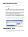
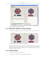
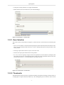
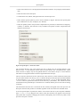
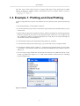
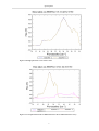
SPIRE SpecExplorer User Manual
Khobaib Zaamout
SPIRE-BSS-DOC-003173
Version 0.0
November 28, 2008
SPIRE SpecExplorer User Manual
Khobaib Zaamout
Table of Contents
1. SpecExplorer ............................................................................................................
1.1. Starting SpecExplorer ......................................................................................
1.2. SpecExplorer Layout .......................................................................................
1.2.1. Bolometer Detector Arrays Display .........................................................
1.2.2. Control Panel .......................................................................................
1.2.3. Preferences Panel .................................................................................
1.3. Example 1: Plotting and OverPlotting .................................................................
1.4. Example 2: Making a Thumbnail Image ..............................................................
iii
1
1
1
2
2
4
6
8
Chapter 1. SpecExplorer
The Spectrometer Detector Explorer, also known as SpecExplorer, is a GUI-based visualization tool
that allows efficient inspection of the contents of the two SPIRE products: Spectrometer Detector
Interferogram (SDI) and Spectrometer Detector Spectrum (SDS). The following sections detail the
features of SpecExplorer.
1.1. Starting SpecExplorer
SpecExplorer is an application that can be called from the interactive data processing environment
HIPE. At least one instance of one of the classes Spectrometer Detector Interferogram or Spectrometer
Detector Spectrum must already be available in memory. For example, such a product can be loaded
into memory via the Product Access Layer.
In HIPE, identify the product for visualization from the Products list and right-click the Spectrometer
Detector Interferogram or Spectrometer Detector Spectrum product, follow the “Open With” menu
entry and select the SpecExplorer from the drop-down menu (see Figure 1.1).
The SpecExplorer can also be called from the command line. SpecExplorer will visualize any Spectrometer Detector Interferogram (SDI) or Spectrometer Detector Spectrum product (SDS). In the HIPE
command line window, we will load a product of the name SDS after entering the following commands:
>from herschel.spire.ia.dataset.gui import SpecExplorer
>SpecExplorer(myProduct)
Figure 1.1. Starting the SpecExplorer via HIPE.
1.2. SpecExplorer Layout
The Graphical User Interface of the SpecExplorer is divided into four sections: The Bolometer Detector Arrays Spectrometer Long Wavelength (SLW) on the top to the left, the Spectrometer Short
Wavelength (SSW) on the top to the right. The Control Panel is on the bottom left and the Preferences
Panel are on the bottom right (see the Figure 1.2).
1
SpecExplorer
Figure 1.2. SpecExplorer Graphical User Interface.
1.2.1. Bolometer Detector Arrays Display
The top panels of the SpecExplorer contains the display of the two detector arrays, (see Figure 1.3)
Figure 1.3. SpecExplorer – Bolometer Detector Arrays Display.
This display allows the user to select any of the detectors of the SPIRE spectrometer: The long wavelength array on the left and the short wavelength array on the right. The detector layout reflects their
arrangement in a honeycomb pattern. Clicking on one or more of these detectors allows the user to
plot the data said detector recorded.
1.2.2. Control Panel
The Control Panel (see Figure 1.4) allows users to
• Select a subset of the scans within the data product (Scan Selection).
2
SpecExplorer
• Create plots of many datasets on one page (Thumbnails).
• Define the fill colors for the detectors (Color Scheme Range).
Figure 1.4. SpecExplorer - Control Panel.
1.2.2.1. Scan Selection
This section of the Control Panel (see Figure 1.5) allows the user to select the scans for which to plot
data:
• The Forward and Reverse buttons allow the plotting of scans based on the direction of those scans.
Since all scans should be either forward or reverse, checking both options will plot all the scans
in one product.
• The Single option allows the user to plot one scan at a time.
• The All Scans option plots all the scans in one product.
• Free Text: Users can specify a range of scans to be plotted in a free text field. For example, if the
user wishes to plot scans 1 through 4 and scans 7 and 8, this can be specified as follows in the user
selected scans section: 1-4 7,8. The wildcard * will select all scans.
Figure 1.5. Control Panel - Scan Selection.
1.2.2.2. Thumbnails
The SpecExplorer allows the user to plot data recorded by many detectors during one observation on
a single page to compare data more effectively. The resulting data plots are small in order to fit all
3
SpecExplorer
requested plots on one page, leading to "thumbnail" images of the data. The result is a single page
which contains a number of thumbnail data plots arranged in the same pattern as the detectors are
presented in the Bolometer Detector Array display, a honeycomb pattern. The scaling of the main plot
window is applied to each thumbnail image. If no plot window is currently open, the selection of the
Initial Scale on the Preferences Panel is applied. Three selections are available under the Thumbnail
drop-down menu (see Figure 1.6):
1 SLW to plot data which were recorded by the detectors in the long wavelength detector array. Depending on the selection in the Preferences Panel, data are shown only for the nominal or unvignetted detectors.
2 SSW to plot data which were recorded by the detectors in the short wavelength detector array. Depending on the selection in the Preferences Panel, data are shown only for the nominal or unvignetted detectors.
3 Co-Aligned to plot data which were recorded by the co-aligned detectors in SLW and SSW. Depending on the selection in the Preferences Panel, data are shown for all the nominal or only the
unvignetted co-aligned detectors.
Figure 1.6. Control Panel – Thumbnails – Thumbnails Selections.
1.2.2.3. Color Scheme Range
This section allows the user to change and control the color scheme used to determine the colors used in
the honeycomb "images" for the Detectors Display (see Figure 1.7). Two color schemes are available
which both go from white (high values) to black (low values): Grey Scale and Heat. The values for the
color scheme are set to the average of the detector data within a user-specified data range. The range
slider, and the indices and values displayed next to it, specify the abscissa range in the interferograms
or spectra which is used to compute the average signal value and subsequently set the colors. Note
that only the abscissa indices, not the values, can be entered by the user.
Figure 1.7. Control Panel - Color Scheme.
1.2.3. Preferences Panel
This panel (see Figure 1.8) allows the user to
4
SpecExplorer
• Select which detectors are to be displayed in the Bolometer Detector Array Display and the Thumbnails.
• Select the initial scale of the plots.
• Customize the title, subtitle, and legend entries for the main plot area.
• Select whether spectral phase is given in units of radians or degrees. Note that the spectral phase
φ(S) is defined as tan φ (S) = Imaginary (S) / Real (S).
• Select the quantity used in the plot when complex data are presented, to either Real or Imaginary,
or Phase, or Absolute. This selection is only available if the product contains complex data with
imaginary and real part.
Figure 1.8. SpecExplorer - Preferences Panel.
The “Nominal detectors only” option allows the user to display only the nominal detectors in the
detector arrays, i.e. those detectors which make sky observations. The “Unvignetted only” option
allows the user to display only the unvignetted detectors in the detector arrays, i.e. those detectors
which have an unvignetted Field of View through the Herschel telescope.
The two selection check boxes for the “Initial scale” allow the user to select whether the initial scale
of a plot reflects the last user choice (“User”) or whether the plot presents the optical passband defined
by the instrument, i.e. 10 – 35 cm-1 for data from SLW and 25 – 55 cm-1 for data from SSW and 10
– 55 cm-1 if data are plotted from detectors from both arrays (“Passband”). The ordinate will scale
with the data for the passband option. If neither box is checked, then the plot will self-scale according
to the data.
The edit buttons allow the user to customize the title, subtitle, and legend of the main plot area. All
descriptors from the data product are available regardless of the level where the metadata reside.
In case the spectral phase is plotted, the “Phase” section allows the user to plot the phase in Radians
from - π / 2 to + π / 2 or in Degrees from -180° to 180°. This selection only applies to the first time
when phase data are plotted. Changing this selection subsequently does not have any effect on the
plot until a new plot is created.
5
SpecExplorer
The “Plot Type” section allows the user to specify which aspect of the spectral flux is plotted
where it is given as a complex number. The absolute value of a complex number is given by
1.3. Example 1: Plotting and OverPlotting
In order to inspect data from a specific scan and detector from a specific product, perform the following
steps:
1 Start the SpecExplorer for the product in question.
2 In the Scan Selection section of the Control Panel specify which scan(s) should be plotted, e.g. all
reverse scans.
3 In the Preferences Panel click the buttons for titles, subtitles, and legends to customize these fields.
Fields are populated by the entries in the inspected product and free text can be added by the
user. Default title, subtitle, and legend information are stored and can be retrieved through the
customization window. See the Figure 1.9:
4 In the Preferences Panel, select the Initial Scaling needed, e.g. Passband.
5 In the Preferences Panel, select the Plot Type, e.g. the Absolute value of a complex number.
6 In the Detectors Display shown in Figure 1.2, single left mouse click the detector to plot its data,
e.g. SLWD3. A new PlotXY window will open with the SSWD3 detector plotted as shown in
Figure 1.10
7 For an overplot, simply double-click with the left mouse button on an additional detector to plot
its data, e.g. SSWC2 (see Figure 1.11). A single click would have created a new plot containing
data from SSWC2 only.
Figure 1.9. Edit Title
6
SpecExplorer
Figure 1.10. Single plot of the reverse scans 1 and 3
Figure 1.11. Overplot of data from two different detectors in two different detector arrays
7
SpecExplorer
1.4. Example 2: Making a Thumbnail Image
In order to compare data from different detectors on the same page perform the following steps:
1 Start the SpecExplorer for the product in question.
2 In the Scan Selection section of the Control Panel specify which scan(s) should be plotted, e.g.
scan number 1.
3 Open the main plot window by performing the steps in Section 1.3, select the range to be plotted
on the thumbnail images , e.g. from 25 cm-1 to 40 cm-1.
4 In the Preferences Panel check whether to get thumbnail images from all, only the nominal, or only
the unvignetted detectors, e.g. “Unvignetted only”.
5 From the Thumbnails drop-down menu on the Control Panel, select to get thumbnail images from
SLW, SSW, or the co-aligned detectors on SLW and SSW (see Figure 1.12 below).
Figure 1.12. Thumbnail images of the unvignetted SSW detectors in the spectral region selected in the main
plot window
8