Download PACS Map-making Tools: Analysis and - Herschel

Document:
Date:
Version:
PACS
Herschel
PACS-mapmaking
November 1st 2013
1.0
Page 1
PACS Map-making Tools: Analysis and Benchmarking
Coordinator and report compiler:
Roberta Paladini
Authors:
(Alphabetical order:) Babar Ali, Bruno Altieri, Zoltan Balog, Alexandre Beelen,
Stefano Berta, Pierre Chanial, Javier Gracia-Carpio, Vera Könyves,
Gabor Marton, Roberta Paladini, Pasquale Panuzzo, Lorenzo Piazzo,
Helene Roussel, Roland Vavrek, Michael Wetzstein
Summary
The PACS photometer blue (70 µm, 100 µm) and red (160 µm) detectors are bolometers.
This type of detectors has noise characterized by a power spectrum that rises at low temporal
frequencies (often referred to as 1/f noise). The removal of 1/f noise typically takes place during
the map-making process, i.e. the process of turning time-ordered data (hereafter, TOD) into
an image in the sky. If the correction for 1/f is not accurate, stripes, even severe, are left in the
final maps compromising their quality. In addition to correct for 1/f noise, the map-making
process also removes from the signal the bolometers common mode drift. This step of data
reduction is typically denoted pre-processing, as it occurs prior to correction for (uncorrelated)
1/f.
In this report, we summarize the results obtained from the comparison of the performance of
six map-making packages for PACS photometer data. The codes which participated in this
exercise are, in alphabetical order: JScanam, MADmap, SANEPIC, Scanamorphos, Tamasis
and Unimap. All these codes are publicly available and are designed to correct for noise in the
data, while preserving emission on all angular scales.
To test the performance of the individual map-making codes, we used a combination of simulated data and real PACS observations. The simulated data were obtained by co-adding a
synthetic sky signal to pure instrument noise. The input sky model is a single image which is
being scaled to the faint and bright background cases. Point sources are also included in the
simulations. However, their flux is not scaled along with the background, hence the source-tobackground contrast is higher in the faint background case. In total, we generated 2 simulated
data sets for the nominal and orthogonal scanning directions. Readers should be aware that,
at this time, the synthetic data do not account for detector dynamic (i.e. finite time constant),
on-board compression and pointing jitter effects.
The simulations described above were complemented by 10 real PACS data sets, selected from
the archive in order to cover a parameter space as wide as possible. In particular, we considered:
PACS
Herschel
Document:
Date:
Version:
PACS-mapmaking
November 1st 2013
1.0
Page 2
faint and bright background sources; galactic and extra-galactic fields; scan and parallel mode
observations; small and large maps; shallow and deep programs.
The test campaign was carried out using a set of 5 different metrics, namely:
1. Power spectrum analysis;
2. Difference matrix;
3. Point source photometry: bright and faint sources;
4. Extended emission photometry: comparison with ancillary data sets (IRAS, Spitzer/MIPS);
5. Noise analysis.
The result of the metrics are summarized below and in Table A:
Removal of emission on some angular scales: no significant flux removal on scales larger
than a few instrument beams is found for any of the mappers. The only exception is represented
by MADmap for the faint background case, both in the blue and red band, for which we report
a slight flux removal at relatively large angular scales;
Point-source photometry: in the bright flux regime (0.3 - 50 Jy), all mappers provide flux
measurements consistent (within 5% - 10%) with High-Pass Filtering (HPF). For fainter fluxes
(0.001 - 0.1 Jy), in the blue band all mappers are in agreement with HPF down to 0.03. In the
red band, the agreement with HPF is found only down to 0.3 Jy, i.e. an order of magnitude
higher than in the red band. The only exception, for both the bright and faint flux regime,
and both the blue and red band, is SANEPIC, for which larger discrepancies with respect to
HPF are evidenced by this photometric analysis. Finally, we find no indication, at this stage,
that any of the mappers allows us to reach a higher flux depth compared to HPF;
Extended emission photometry: no systematic discrepancy, neither in the red nor in the
blue band, is found for any of the mappers from comparison of PACS re-processed data with
ancillary IRAS or Spitzer/MIPS data. At 100 µm all the mappers are typically within 10%
from the IRAS measurements, with the only exception of MADmap which is an outlier with
a 30 % discrepancy. At 70 and 160 µm, PACS re-processed data are on average within 10%
to 40% with respect to the MIPS data, with the largest discrepancies due to residual artifacts
(e.g. stripes) in the MIPS data;
Noise: for the faint background case and in the blue band, Tamasis and Scanamorphos are the
mappers which introduce less noise, although of correlated type, while the other mappers tend
to be characterized by higher uncorrelated noise. In the red band, all the mappers introduce
correlated noise. Furthermore, in both the blue and the red band, for all the mappers the noise
is typically more pronounced along the scan direction (e.g Tamasis in the blue band), with
Document:
Date:
Version:
PACS
Herschel
PACS-mapmaking
November 1st 2013
1.0
Page 3
Metric
JScanam
MADmap
SANEPIC
Scanamorphos
Tamasis
Unimap
Power spectrum
Difference matrix
Bright point source photometry
Faint point source photometry
Comparison with IRAS
Comparison with MIPS
Noise analysis
Global assessment
5
5
4.5
3.9
5
4.5
3
30.9
4.5
3
4.5
3.5
3.5
3.9
3
25.9
5
—
3
2.5
5
3.5
4.3
23.3∗
5
3.7
4.5
3.7
5
4.8
4.7
31.6
5
3.3
4.5
3.6
5
4.5
4
29.9
5
4
4.5
4.2
5
4.7
4.5
31.9
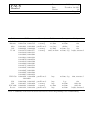
Table A: The grades are from 0 to 5, with 0 denoting the minimum grade, and 5 the maximum.
∗
Note that SANEPIC did not take part in one of the metrics, e.g. difference matrix.
the positive exception of Scanamorphos and Unimap, in the red band, for which the noise is
almost isotropic. The difference maps also show that these two mappers (e.g. Scanamorphos
and Unimap) have the lowest high-frequency (i.e. pixel-to-pixel) noise. Finally, we found that
some of the mappers appear to introduce a gain in flux calibration, especially MADmap for
faint background data, both in the blue/red bands.
Table A is an attempt to provide a preliminary assessment of the performance of the mapmaking codes in light of the metrics described above. For each metric, we evaluated the average
performance of a given mapper based on the plots and discussions included in Section 5 of the
report, and accordingly assigned a grade from 0 to 5, where 0 corresponds to the minimum
grade and 5 to the maximum one. We caution the reader against any straightforward
interpretation of the grades in the Table. Despite an effort of folding in the grades
the nuances of the metric results, it is understandable that a high level of subjectiveness is involved in the process. Therefore, we highly recommend reading
Section 5 ("Codes Benchmarking") and Section 6 ("Conclusions") before coming
to any strong conclusions about the performance of the various mappers.
Document:
Date:
Version:
PACS
Herschel
PACS-mapmaking
November 1st 2013
1.0
Page 4
PACS Map-making Tools: Analysis and Benchmarking
Abstract
In this report, we summarize the results obtained from comparing the performance of
six map-making packages for PACS photometer data. The codes which participated in
this exercise are, in alphabetical order: JScanam, MADmap, SANEPIC, Scanamorphos,
Tamasis and Unimap. All these codes are publicly available and are designed to correct for
noise in the data, while preserving emission on all angular scales. To test the performance
of these codes, we considered a combination of simulated and real data, and a set of five
different metrics, namely: 1. power spectrum estimation; 2. difference matrix; 3. point
source photometry (for both bright and faint sources); 4. comparison with ancillary data
(IRAS and Spitzer/MIPS); 5. analysis of the noise. The analysis evidences that all the
codes preserve emission on large angular scales and that they are able to handle the PACS
data with a high level of photometric accuracy. Finally, we point out that differences in
the generated maps are typically small yet noticeable.
1
Context
The PACS photometer blue (70 µm, 100 µm) and red (160 µm) detectors are bolometers.
This type of detectors has noise characterized by a power spectrum that rises at low temporal
frequencies (often referred to as "1/f noise"). The removal of 1/f noise typically occurs during
the map-making process, i.e. the process of turning time-ordered data (hereafter, TOD) into
an image in the sky. If the correction for 1/f is not accurate, stripes, even severe, are left in
the final maps compromising their quality.
In March 2012 we started a comparison exercise of six different map-making implementations
for bolometer detectors. These implementations were specifically conceived for Herschel PACS
and/or SPIRE timelines, with the exception of the SANEPIC package which was initially
designed to treat data from the BLAST balloon-borne experiment (see Section 2.3). The
preliminary results of the analysis were shown at a dedicated workshop which took place at
ESAC (Spain) on January 28 - 31 2013 (9). The codes performance investigation continued
after the workshop. In this time period, the workshop results were carefully validated and, when
necessary, updated with new results. This document intends both to summarize the methology
used for the comparison exercise and to present the current status of the analysis results. We
emphasize that the developers of the codes whose performance is here under investigation have
actively participated in the testing process and are all co-authors of the document.
The report is organized as follows. In Section 2 we briefly review the characteristics of each
map-making code. In Section 3 we describe how the simulated data were generated, and the
selection of archival observations. In Section 4 we provide details on data processing for each of
the participating mapper. In Section 5 we discusses the benchmarking analysis and its results.
Finally, we summarize our conclusions in Section 6.
PACS
Herschel
Document:
Date:
Version:
PACS-mapmaking
November 1st 2013
1.0
Page 5
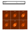
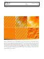
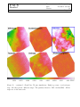
Figure 1: PACS 160 µm scan mode data for the Crab processed by the six map-making codes.
PACS
Herschel
Document:
Date:
Version:
PACS-mapmaking
November 1st 2013
1.0
Page 6
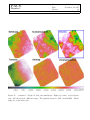
Figure 2: PACS 160 µm parallel mode data of M31 processed by the six map-making codes.
PACS
Herschel
2
Document:
Date:
Version:
PACS-mapmaking
November 1st 2013
1.0
Page 7
Overview of map-making codes for PACS
Figure 1 and 2 illustrate examples of the processing of PACS data sets by the six map-making
tools that we consider for this analysis. Below, we provide a brief overview of these packages.
2.1
JScanam
JScanam is the Hipe/PACS implementation of the Scanamorphos algorithm developed in IDL
by Helene Roussel (http://www2.iap.fr/users/roussel/herschel). As Scanamorphos, it is designed to remove the low frequency noise (also called 1/f noise) typically found in bolometer
arrays, which produces strong signal drifts in the pixel timelines. The algorithm is based on
the following assumptions:
• the drifts power increases with the length of the considered time scale (1/f noise). For
that reason JScanam starts removing the drifts with the longest time scale, beginning
from the scan duration, continuing with the scanleg duration, and finally on time scales
shorter than a scanleg. In each step the remaining drifts are weaker than in the previous
step, which facilitates the drift removal;
• the PACS observations were done in pairs of scans and cross scans with close to perpendicular scan directions. This is necessary because in some of the JScanam tasks
the information from the cross scan is used to remove the drifts from the scan (and vice
versa), and this is only possible when the drifts projections on the sky have perpendicular
directions;
• short term drifts from different bolometers in the array are independent. If the map pixel
size is large enough to include a significant number of pixel crossings at different times
and from different bolometers, the drifts average contribution to the map should be close
to zero.
If these three conditions are fulfilled, the JScanam tasks are able to remove most of the 1/f
noise from the PACS photometer signal, preserving the flux from real sources at all spatial
scales (shorter than the map size). We should note that even if they are based on the same
principles, the JScanam and Scanamorphos implementations are quite different in many points
and assumptions. This explains why they do not produce always the same results.
2.2
MADmap
The Microwave Anisotropy Dataset mapper (MADmap) is an optimal map-making algorithm,
which is designed to remove the uncorrelated (1/f) noise from bolometer time ordered data
(see (5)). The removal of 1/f noise creates final mosaics without any so called banding or
striping effects. For Herschel data processing, the original C-language version of the algorithm
has been translated to Java to comply with HIPE requirements. Additional interfaces are in
place to allow PACS (and SPIRE) data to be processed by MADmap. This implementation
requires that the noise properties of the detectors are determined apriori. These are passed to
PACS
Herschel
Document:
Date:
Version:
PACS-mapmaking
November 1st 2013
1.0
Page 8
MADmap via PACS calibration files and are referred to as the InvNtt files or noise filters. The
InvNtt is short for Inverse Time-Time Noise correlation matrix.
2.3
SANEPIC
Signal And Noise Estimation Procedure Including Correlation (sanepic) is a maximum likelihood mapper capable of handling correlated noise between receivers. It was first developped to
handle the BLAST experiment data (16), and then fully rewritten, parallelized, and generalized
to handle any kind of dataset. The sanepic package now consists of several programs:
• saneFrameOrder : finds the best distribution of the input data files over several
computer, if sanepic is used on a cluster of computers;
• sanePre : distributes the data to temporary directories. The data are stored in a dirfile
format, each computer receiving the data segment it will process;
• sanePos : computes the map size, pixel indices and a naive1 map. One can define a
projection center or use a mask as a reference for projection. Users can use all projection
supported by wcslib (4; 7). The conversion to/from ecliptic and galactic coordinates is
also possible. A mask for strong sources can also be define to remove crossing-constraints
between different datasets;
• sanePS : computes noise-noise power spectra. The data are pre-processed and decomposed, in the Fourier domain, into uncorrelated and n-correlated components, using a
mixing matrix of the correlated component, all components, common noise power spectra and mixing coefficients, are found using an expectation-maximization algorithm ;
• saneInv : inverts the noise-noise power-spectra by mode, as needed for the full inversion
made by sanePic;
• sanePic : iteratively computes the optimal map using a conjugate gradient method.
All programs take inputs from a single ini file which describe all parameters, in particular
the frequency of the high-pass filtering needed before being able to transform the data in the
Fourier domain (see Section 4.3.1 for limitations).
2.4
Scanamorphos
Scanamorphos is an IDL software making maps from flux- and pointing-calibrated time series,
exploiting the redundancy in the observations to compute and subtract the total low-frequency
noise (both the thermal noise, strongly correlated among detectors, and the uncorrelated flicker
noise). The required level of redundancy is reached in PACS observations; a fiducial value that
is convenient to remember is 10 samples per scan pair and per FWHM/4 pixel. Its capabilities
1
In a naive map, the data are simply re-mapped onto the image plane, with no additional data processing
on the timelines.
PACS
Herschel
Document:
Date:
Version:
PACS-mapmaking
November 1st 2013
1.0
Page 9
also include the detection and masking of glitches, and of brightness discontinuities caused
by either glitches or instabilities in the multiplexing circuit; low-level interference patterns
sometimes affecting PACS data are not handled. The algorithm is described, accompanied by
simulations and illustrations, in (24) and (25). The repository of the software and up-to-date
documentation is: http://www2.iap.fr/users/roussel/herschel . The output consists of a FITS
cube, of which the third dimension is the plane index. The first plane is the signal map; then
comes the error map (statistical error on the weighted mean), the subtracted drifts map and the
weight map. The weight of each sample is the inverse square high-frequency noise (one value
for each bolometer and each scan). Whenever present, the fifth plane is the "clean" signal map,
where the mean signal from each scan has been weighted by its inverse variance; it is provided
to ease the detection of remaining artefacts in the map (by comparison with the first plane),
not for scientific purposes.
2.5
Tamasis
Tamasis stands for Tools for Advanced Map-making, Analysis and SImulations of Submillimeter
surveys. It is an ASTRONET funded project aiming at providing reliable, easy-to-use, and
optimal map-making tools for Herschel and future generation of sub-mm instruments. The
project is a collaboration between 4 institutes (ESO Garching, IAS Orsay, CEA Saclay, Univ.
Leiden). Tamasis code is massively parallel (MPI + OpenMP) and is written in FORTRAN
(for the number crunching) and Python (for the abstraction easiness). Tamasis is publicly
available to the community2 . Tamasis is used not only to reconstruct optimal maps, but also
to manipulate timeline data and to compute maps with naive projection.
2.6
Unimap
Unimap is a map maker based on the Generalised Least Square (GLS) approach, which is also
the Maximum Likelihood (ML) method when the noise has Gaussian distribution. The method
is known since the ninetiees, e.g. (26), and several practical implementations were proposed in
the last decade. Unimap is specialised for handling Herschel data (PACS and SPIRE).
Unimap is written in Matlab and can be compiled to run on every machine where Matlab can
be installed, including Windows, Linux and Mac. Note that it is not required that Matlab is
installed to run Unimap. Only some runtime libraries are needed.
Unimap (version 5.5) is divided into several modules, which are summarised in the following:
• Data loading: the input data to Unimap is a set of fits files, each one storing an
observation. The first module performs the loading of these files and creates the internal
data structures, including the projection of the data onto the pixellized sky, defined by
the astrometry parameters. This module also takes care of performing an initial filtering
of the data, by rejecting timelines with a percentage of flagged redaouts higher than a
user-specified threshold, and of setting the unit measure as specified by the user;
2
http://pchanial.github.com/pyoperators and http://pchanial.github.com/tamasis-map
PACS
Herschel
Document:
Date:
Version:
PACS-mapmaking
November 1st 2013
1.0
Page 10
• Pre-processing: this module detects signal jumps due to cosmic rays. Where jumps are
detected the data are flagged and the timeline is broken into two, independent timelines.
The module may also remove an initial signal tilt due to the memory of the calibration
block, which can be found at the beginning of the timelines. As a last step, the module
linearly interpolates the flagged data;
• Glitch: this module performs a high-pass filtering of the timelines and carries out a
glitch search on the high-pass filtered data. A sigma-clipping approach is used according
to which, for each pixel, the outliers, i.e. readouts with a difference from the median value
larger than a user-selectable multiple of the standard deviation, are marked as glitches.
After detection, the marked values are reconstructed using linear interpolation;
• Drift: this module estimates and removes the polynomial drift affecting the timelines.
It exploits an Iterative implementation of a Subspace Least Square approach (? ). The
user can select the polynomial order and decides if the drift is to be estimated for every
single bolometer or for a whole array/subarray;
• Noise: this module estimates the noise spectrum and constructs the corresponding GLS
noise filters;
• GLS: this module estimates and removes the noise affecting the timelines by implementing the GLS map maker. It produces two output images in the form of fits files: the naive
map and the GLS map;
• PGLS: this module estimates the distortion introduced by the GLS map maker. It is
based on the Post-Processing for GLS (PGLS) algorithm described in (17). The estimated
distortion is subtracted from the GLS map to produce a PGLS map, which is saved in
the form of a fits file;
• WGLS: this module implements the Weigthed PGLS (WGLS) described in (17) where
the distortion estimated by the PGLS is analysed and subtracted from the GLS image
only when it is significant. In this way the noise increase caused by PGLS is minimized.
A more detailed description of the map maker can be found in the user’s manual, which can
be downloaded from the Unimap Home Page (28).
3
Benchmarking data set
To test the performance of the individual map-making codes, we made us of both (hybrid)
simulated and real PACS observations.
3.1
Hybrid simulated data
The map-makers performance can be accurately tested on hybrid simulated data in which
simulated sky signal and pure instrument noise components are co-added in the flux calibrated
PACS
Herschel
Document:
Date:
Version:
PACS-mapmaking
November 1st 2013
1.0
Page 11
Level 1 detector timeline. As a result of the map-making process, an ideal projected map carries
only sky signal, while the noise component is being separated by the projection algorithm. This
hypothesis can be well tested by comparing the unbiased input sky model with a compromised
quality projected map. Deviations from the sky model qualifies the map-making process and
can be used to characterize the spectral response of the map-maker.
3.1.1
Hybrid simulations components
Hybrid simulations are made up of three components:
1. Noise donor calibration observation. A long staring observation at a low FIRbackground position of the sky. This dataset consists of pure instrument 1/f noise and
telescope background measured for a nominal detector setup (detector bias and readout
mode). A section of this noise sample is copied into the flux cube of the receptor science
observation;
2. Receptor science observation. Placeholder of the simulated dataset. Its flux cube is
cancelled out, the noise donor replaces the Level 0 timeline of the science data frames,
when reaching processing Level 1 the sky model is superimposed over the timeline. The
AOT setup is typical for a PACS scan-map observation in terms of scan-speed, redundancy
(map repetitions) and observing strategy (multiple coverages at orthogonal scan angles).
In addition, the spacecraft attitude has been reconstructed on the best effort basis using
the ICC pointing reconstruction algorithm under development (includes gyro drift- and
sub-pixel correction). The residual pointing reconstruction error is considered as low as
0.1"-0.3" rms;
3. Sky model donor image. A realistic sky model, image either a superior quality measured dataset or a simulated image. The pixel size of the input sky map (model sky
granularity) should not be larger than half the pixel size in the final projected map.
3.1.2
Generation of simulated data
The simulated Level 1 hybrid cubes consist of three components:
1. Noise donor cube: a staring calibration observation originally designed for detector lowfrequency noise characterization over the ISOPHOT dark-field. This allows the simulation
of PACS instrumental noise;
2. Receptor science observation: a 35x35 arcmin observation taken at nominal- and
orthogonal scan directions with single map repetition and 20"/sec scan speed. This setup
is considered being a representative PACS large-field observation;
3. Sky model: 2D-pink-noise simulation representative for sky cirrus observations. The
surface brightness is adjusted to generate bright and faint cases. Point-sources of uniform flux distribution are superimposed over this simulated image. The faint and bright
background cases differ by a factor 3 in surface brightness.
PACS
Herschel
Document:
Date:
Version:
PACS-mapmaking
November 1st 2013
1.0
Page 12
The sky-model map are fine sampled (pixel of 1"), convolved with Gaussian beams (sampled
by 1" pixels), and scaled to the desired brightness. The simulation procedure is as follows (see
Figure 3):
• Take Level-0 data of a real PACS observation of a dark field (i.e. the noise donor) and
copy into the Level 0 flux cube of the receptor observation;
• Add improved pointing product to receptor observation;
• Run pipeline (HIPE v11.876) on receptor cube up to Level 1 frames generation. This will
produce flux-calibrated 1/f noise timeline;
• Create WCS for input sky model, as well as standard WCS for projections (based on the
receptor cube footprint);
• Calculate map-index: obtain the RA and DEC for every sampling point in the Level-1
timelines of the receptor cube, then assign pixels from the sky-model map at the RA and
Dec of a given sampling point in the receptor timeline. Map-indexing takes into account
the fractional overlap of detector pixels and sky model pixels. Map-indexing from L2 sky
model to L1 receptor cube has been done with pixfrac=1.0;
• Apply broad-width (100) High-Pass Filter (HPF) on the receptor cube with pure instrument noise. Using photProject() and the input sky WCS, project this cube noise with
pixfrac=0.1;
• From the above created noise-map, determine suitable scaling factors required for bright
and faint simulation cases;
• Create a point-source catalogue of uniformly distributed fluxes in the [10.0 - 500.0] mJy
range and produce source images; convolve the sky model as well as the point-source
images with Gaussian PSFs and create composite images used for timeline projection;
• Using the map-index, project the sky simulation composite images onto an L1 flux cube;
• Using the standard projection WCS, project with photProject the L1 pure sky simulation
flux cube with pixfrac=0.1. This will serve as the reference map containing the pure
geometrical footprint of the naive projection mechanism;
• Correct for digitization effect to simulate proper quantization noise;
• Co-add noise- and projected sky model flux cubes and copy back to Level 1 simulated
cubes;
• Create Observation Context with simulated Level 1 cubes.
PACS
Herschel
Document:
Date:
Version:
PACS-mapmaking
November 1st 2013
1.0
Page 13
Figure 3: Intermediate steps of the simulation process from top-left to bottom-right: map1 pure noise donor cube projected onto input sky WCS (1" pixel size); map2 - the same as map1
but after applying HPF with filterSize=100; map3 - jaive projection of pure sky model cube
onto standard projection WCS (3" pixel size in the red band); map4 - pure noise donor cube
projected onto small input WCS after applying HPF; map5 - similar to map1 but projected
onto larger pixelseize standard projection WCS; map6 - naive projection of sky+noise cube
applying HPF on the timeline.
PACS
Herschel
Document:
Date:
Version:
PACS-mapmaking
November 1st 2013
1.0
Page 14
Figure 4: Summary of PACS Type-2 simulation components.
3.1.3
Final simulated data sets
We decided to restrict the PACS simulations parameter space to a single simulation attribute:
the extended emission brightness. The input sky model is a single image which is being scaled
to the faint and bright map cases. The point-source fluxes do not change, i.e. the source-tobackground contrast is larger in the faint simulation case. In total, we generated 2 simulated
Level 1 data sets for the nominal- and orthogonal scanning directions. The components of the
simulation are summarized in Figure 4.
3.1.4
Common WCS for model- and projected map
Irrespective of the photometric band, the PSF convolved input sky simulations are provided
on a common WCS with a pixel size of 1".
3.1.5
Simulations Caveats
The simulations include representative instrumental noise and outliers due to glitches in the
noise donor dataset. However, they do not include detector dynamics (i.e. finite time constant)
and on-board compression effects. In addition, pointing jitter is not simulated, i.e. an infinite
accuracy knowledge of attitude is assumed. The Level-1 timelines provided by the simulations
are already de-glitched using the standard PACS pipeline, and both 2nd order de-glitch mask
and MMT glitch masks are provided in the simulation L1 frames products.
3.2
Real Data
PACS real data selection was performed to allow us to cover a parameter space as wide as
possible in terms of:
1. source surface brightness;
2. background surface brightness;
PACS
Herschel
Document:
Date:
Version:
PACS-mapmaking
November 1st 2013
1.0
Page 15
3. background morphology;
4. size of sky area covered by the observations;
5. observing mode;
6. depth (i.e. # of repetitions).
Following the criteria above, we selected 10 fields (see Table 1). These cover: galactic (e.g.
LDN 1780) and extragalactic targets (e.g Antennae); scan (e.g. NGC 6946) and parallel mode
observations (e.g. LDN 1780); small (∼ 15’ × 15’, e.g IC 348) and large (a few degrees, e.g.
M31) areas; relatively shallow (e.g. Atlas) and deep (e.g. Abell 370) programs; faint/flat (e.g.
Crab) and bright/structured background (e.g. Rosette). In generating the maps with the
various mapping codes, different pixel sizes were adopted. In particular, for programs covering
large areas of the sky (Atlas, LDN 1780, M31, M81), a pixel size of 3.2" for the blue band and
of 6.4" for the red band were used, while for the rest of the programs the pixel size was set
to 2" for the blue band and to 4" for the red band. The only exception is represented by the
Abell 370 data set, for which a pixel size of 1.2" and 2.4" was used, for the blue and red band,
respectively.
4
4.1
Data Processing overview
JScanam processing
The processing of the simulated and real PACS data was done with the latest version of the
JScanam tasks included in Hipe 11. The JScanam package comes with an accompanying
pipeline script that can be easily accessed through the Hipe menu (Photometer/Scan map
and minimap/Extended source JScanam/scanmap Extended emission JScanam). The script
processes the data from a Level 1 HSA product to a Level 2 projected map. It comes with a set
parameters that can be modified by the user, but the proposed defaults produce satisfactory
results in most cases. For this comparison exercise, the default parameters were used for almost
all datasets. In particular, the galactic option was always set to true, even in those cases were
the emission was concentrated on a small region. The drift removal is implemented in two
separate tasks: scanamorphosDestriping() and scanamorphosIndividualDrifts(). The first one
removes drifts from the signal with time scales longer than a scanleg, while the second one
works on shorter time scales. Before these two tasks are executed, some data pre-processing
is required. Strong signal jumps produced by cosmic ray hits on the electronics are identified
and masked. Frames affected by strong drifts produced after the observation of the calibration
source are also masked. An especially important pre-processing step is the creation of a good
source mask. This mask is used by several JScanam tasks, but it is particularly important for
the scanamorphosDestriping() task, where small pointing offsets between the scan and cross
scan can produce significant effects close to bright sources, if they are not masked. A good
source mask should include the brightest sources, but does not need to include all the extended
emission. It should never cover more than one third of the map.
Document:
Date:
Version:
PACS
Herschel
PACS-mapmaking
November 1st 2013
1.0
Page 16
Field
OBSIDs
Obs. mode
Field size
Coverage
Background
Abell 370
Antennae
Atlas
Crab
IC 348
1342223332, 1342223333
1342187836, 1342187837
1342189661, 1342189662
1342204441, 1342204443
1342238774,1342238775
1342238830,1342238831
1342239043,1342239044
1342239433,1342239434
1342240719,1342240720
1342241389,1342241390
1342241460,1342241461
1342241515,1342241516
1342241647,1342241648
1342241697,1342241698
1342241927,1342241926
1342242058,1342242059
1342224989, 1342224990
1342224991
1342211604, 1342211605
1342186085, 1342186086
1342204421, 1342204422
1342186121, 1342186122
scan map
scan map
parallel mode
scan map
scan map
small
medium
very large
medium
small, medium
deep
medium
shallow
medium, deep
medium, deep
flat
flat
flat
flat
bright, structured
parallel mode
large
medium, deep
faint, structured
parallel mode
scan map
scan map
parallel mode
large
large
medium
large
deep
medium
medium
medium
flat
fairly flat
fairly flat
bright, structured
LDN 1780
M31
M81
NGC 6946
Rosette
Table 1: Summary of the real PACS data sets involved in the map-making codes benchmarking.
PACS
Herschel
4.1.1
Document:
Date:
Version:
PACS-mapmaking
November 1st 2013
1.0
Page 17
Processing notes
The main current limitation of JScanam is its large memory requirements. Around 90 GB of
memory were necessary to reduce the bigger fields (Atlas map), but most maps can be reduced
with less than 10 GB. The latest version of JScanam, to be included in Hipe 12, has improved
in this respect, and requires half of the memory than the Hipe 11 version.
4.2
MADmap processing
NOTE: Some of the images produced via the MADmap pipeline for this report did not have
optimal signal drift correction in the pre-processing stage (see the discussion below on preprocessing). The resulting maps show significant sloping backgrounds, which affect pixel-to-pixel
and differenced image metrics most strongly. The photometry from these maps is consistent with
expectations and is considered reliable. The artifacts are a result of improper pre-processing of
timelines resulting from the time constraints imposed by the report schedule, and the interactive
nature of processing requirement by the pre-processing code. These artifacts are not a result of
the GLS algorithm. Future versions of PACS pre-processing code will mitigate these artifacts
for all fields.
The point of using MADmap is to account for signal drifts due to 1/f noise while preserving
emission at all spatial scales in the final mosaic. Thus, the MADmap algorithm, and indeed
most optimal map makers, assume and expect that the noise in the time streams is entirely
due to 1/f variations. The MADmap pipeline processing was started at the Level 1 stage. The
PACS bolometer timelines at this stage contain two additional sources of noise that must be
mitigated before the MADmap algorithm is applied: (i) the PACS bolometers have pixel-topixel electronic offsets in signal values. These offsets must also be homogenized to a single
base level for all pixels prior to combining signals across pixels; (ii) the timelines contain
spatially correlated (pixel-to-pixel correlated) drift in the signal level as a function of time.
The MADmap algorithm assumes that the noise is spatially (i.e. pixel-to-pixel) uncorrelated
and will incorrectly interpret any systematic non-1/f-like drifts as real signal. The removal of
these artifacts is done in the pre-processing stage prior to map-making itself. Each of these
pre-processing steps is discussed below.
• pixel-to-pixel offset correction: for most single channel bolometers the offset is electronically set to approximately 0. The PACS bolometers are, however, multiplexed and
only the mean signal level for individual modules or array can be set to 0, leading to
the observed variations in the pixel-to-pixel signal level. This is purely an electronic and
design effect. Mitigation of this effect entails subtracting an estimate of what the zero
level should be per pixel from each of the readouts of the pixel. The median of the entire
pixel history is used to set the zero-point. The idea is to compute the median of the
entire history of signal values per pixel and subtract this median from each of the pixel
readouts. The task photOffsetCorr() applies this correction in HIPE;
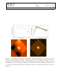
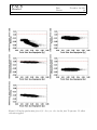
• Global drift correction: Figure 5 illustrates the concept of correlated signal drift. It
shows the median of an individual readout (image) in the observation cube plotted against
PACS
Herschel
Document:
Date:
Version:
PACS-mapmaking
November 1st 2013
1.0
Page 18
time (readout index). The rise and decline of the median signal in Figure 3 is not due
to change in the intrinsic intensity of the observed source, but due to a change (drift) in
the raw signal level that is correlated in time for all pixels. (3) discuss the origin of this
drift as likely due to drifts in the focal plane temperature of the bolometer array. The
observed behavior is usually a monotonic decline but may also be more complex such
as the one shown in Figure 5. Strong astrophysical sources produce "spikes" (rapidly
changing signal) atop the drift signal as the source moves in and out of the field of view
of the array during a scan.
In PACS data processing, the correlated signal drifts are modeled as low-order polynomial.
This requires separating the drift component from any strong astrophysical sources that
are also present in the signal, and further requires user interaction to select appropriate
polynomial model. Timelines that are not properly fit by a single polynomial are subdivided (segmented) in smaller groups to ensure an accurate determination of the baseline.
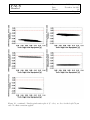
Figure 6 shows two examples of the correlated drift removal with two significantly different
outcomes. The left two panels in Figure 6 show a 2nd order polynomial fit to baseline.
This case is presented to illustrate the difficulty in baseline fitting, and the need for
user-interaction. We do not expect that users are so obviously careless in their data
processing. In this case, the baseline is the minimum value of bins with user-defined
bin widths. The minimum value rejects the signal from the astrophysical source. The
2nd order polynomial, however, provides a poor fit to the baseline, and consequently, the
resulting map (bottom left-hand panel) shows systematic variations in the final image.
The two right-hand side panels in Figure 6 show the results when careful, segmented
mitigation is applied to the data.
The resulting error is dependent on the degree of accuracy achieved in applying polynomial models to the correlated drift. This is difficult to quantify since it depends partly on
user’s due diligence, and partly on how well-behaved is the background drift. Note that
the PACS bolometers show negligible correlated drift towards the end of the observation
day, and data taken during these stable periods requires no correction for the correlated
drift. Experience suggests that projected maps fluxes may be corrupted by as much as
0-30% compared to the best reduction.
For data that are dominated by the background, the trend is relatively easy to model as
source contamination is negligible. However, a more generic approach is needed that is
also able to account for data that contain significant astrophysical emission. To do this,
1000 readout wide bins are created and it is assumed that the minimum values in these
bins corresponds to the few actual blank/background measurements. The idea is that
over these 100 readouts, at some point, the scan pattern observed a sourcefree part of the
sky. This will appear as the minimum value of the bin. The minimum value of each bin
is extracted and the resulting trend in the minimum values is fitted with a polynomial
(usually 2nd or 3rd degree). The best-fitting polynomial is then assumed to described
the correlated global drift and is subtracted from the each readout.
PACS
Herschel
Document:
Date:
Version:
PACS-mapmaking
November 1st 2013
1.0
Page 19
Figure 5: Correlated signal drift of the PACS bolometer signal. The change in signal intensity
over time scales of >100s of readout is due to simultaneous drift in the raw signal intensity
for all pixels of the array. Strong astrophysical sources produce changes on much shorter time
scales as they move in and out of the field of view of the bolometer array during a scan. The
"spikes" seen atop the drift signal are due to sources in the sky.
4.2.1
Processing notes
The pre-processing steps described above were applied to each simulated and real data set. In
some instances, it was necessary to flag and remove additional sections of readouts that showed
artifacts resulting from a cosmic ray hitting directly the electronics. These manifest themselves
as the so-called "module-" or "pixel-" drops, and are recognized as a sudden and drastic change
in the signal level of the module or the pixel, which is sometimes sustained over thousands of
readouts. Once free of artifacts, the MADmap algorithm is applied to the data to remove the
1/f noise and produce a final map.
4.3
SANEPIC processing
All the PACS simulated and real data were processed according to the same procedure, i.e.:
• export the data from HIPE using export_SpireToSanepic.py or export_PacsToSanepic.py
scripts;
• define a blank mask with the requested WCS, add some margin pixels to accommodate
for flag data on the edge, as sanePic need to be able to project all data : even flagged
data needs to be present in the map (although not in the final map);
• write the ini file for the processing, defining all directories, parameters file and choosing
a very low frequency cut (half length of the time-stream allows to );
• distribute the data segments with sanePre and compute pixel indices and a naive map
with sanePos;
PACS
Herschel
Document:
Date:
Version:
PACS-mapmaking
November 1st 2013
1.0
Page 20
Figure 6: Correlated signal drifts in the PACS bolometer timelines (top panels) are fit by
interactive curve-fitting processing. This Figure shows the resulting maps when the fit is
inappropriately (left side) and when drift is mitigated properly (right side). While most users
will likely show due diligence in removing the correlated drift, the resulting systematics may
be noticeable in automatic pipeline processing for which a one-size-fits-all default values are
applied.
PACS
Herschel
Document:
Date:
Version:
PACS-mapmaking
November 1st 2013
1.0
Page 21
• for blank/deep fields, compute the noise-noise power spectra using sanePS with the
raw data, or bootstrap previously computed noise-noise power spectra; the number of
common-mode components varies, i.e. 6 for the PACS green band;
• inverse the noise-noise power spectra with sanePS and run sanePic.
The last two steps can/must be iterated using the previous iteration map of sanePic as an
input to be remove from the time-stream by sanePS. The process converge quickly, in 3 to 4
iterations. This allow to derive noise-noise power spectra in the case where strong or weak
emissions are present in the data. This also allow to adapt the noise component to each data
segment, in particular in case of cooler burps. In case of strong emission in the data, noisenoise power spectra from a previous empty field can be bootstrapped as the first iteration in
the process.
4.3.1
Processing notes
sanepic make several assumptions on the data and nosie model, which can leads to known
caveats/artifacts on the maps :
No gaps in the time stream : processing data in the Fourier domain requires that the timestreams
are contiguous, i.e without gaps, in order to maintain consistency in the noise frequencies
features. In particular, even if they are not used in the final map, turnaround of PACS
data must be present in the timestream;
Signal is circulant : this is an intrinsic hypothesis when doing Fourier Transforms and implies that any signal gradient between the beginning and the end of the timestream will
be removed : if the observation does not end where it started on the sky then any large
scale gradient between those two points will be filtered out. This leads to very large
scale filtering of bright gradient in PACS maps as the observations often start and end
on the two extreme points on the map. Note that apart for very large scales, that are
not measurable by a Fourier analysis of the map, all the other scales are preserved. This
implies that any difference from a truth map will show a large gradient, while any Fourier
analysis of the map will show a transfer function close to unity;
Noise is stationary : the noise properties are described by a single power spectrum for a
given data segment, implying that across the data segment the noise must be stationary,
having the same properties from start to end. This is very well the case for PACS receivers.
If there are strong noise properties changes, one could partition the data segment in several
parts, in which the noise is stationary;
Sky is constant over a pixel : As for all the mapmakers, sanepic assumes that the sky is
constant/flat over a pixel in the final map. This assumption could be broken in the case
of (1) a strong gradient in a single pixel, (2) astrometric mismatch, (3) gain or calibration
mismatch between data segments. These problems, in case of strong sources, could lead to
a wrong determination of the sky level over the filtering length of the data segment, thus
leaving strong artifacts (crosses) on the maps. In order to avoid those problem, sanepic
PACS
Herschel
Document:
Date:
Version:
PACS-mapmaking
November 1st 2013
1.0
Page 22
can remove the crossing constraints, between two data segments, using a mask for strong
sources, whose flux level is determined using a simple mean between data segments;
Bad Data/Glitches/Steps/Moving Objects/... : since sanepic is only a mapmaker, data
must be properly flagged before being projected. Strong glitches, steps or any strong nonphysical gradients (induced from simulations with mismatched background level for e.g.),
not well described in the Fourier domain, will need to be detected and flagged prior
to theprocessing. This could lead strong features in the maps, even crosses, for strong
glitches, or in the case of several faint unflagged glitches, to an overestimate of the white
noise level.
4.4
Scanamorphos processing
The processing options used for each dataset (among /parallel, /galactic, /jumps pacs) can be
found in the fits headers of the processed maps. The log files, available upon request, contain a
summary of the processing steps, drifts amplitudes, observation duration and processing time.
The processing was first done with version 19 of the code.
The glitch mask determined within HIPE was disabled, and the deglitching was done entirely
in Scanamorphos.
4.4.1
Processing notes
After the first processing, a bug was found that prevented the average drift of the first scan
leg of each obsid to be faithfully propagated: in other words, the average drift was correctly
computed but not accurately subtracted. The red band of two PACS real data sets, i.e. NGC
6946 and M81, which were particularly affected by this bug were reprocessed with a revised
version of the code (e.g 20.1). For these fields and band, the improvement in the outer parts
of the map is visible by eye.
4.5
Tamasis processing
Before executing the optimal reconstructions of the maps, the data have to be pre-processed.
The pre-processing is divided in three steps. The first step removes the baseline, i.e. the
drift caused by variations of the detector plate temperature. The second step consists in the
identification and masking of jumps in the timelines. These jumps are caused by glitches in the
electronics (also called “long glitches”). The final step is the second level deglitching to remove
short glitches.
• Baseline removal: As in the case of MADmap, Tamasis optimal reconstruction gives
the best results if correlated trends (or baseline) are removed from the signal timelines
before the reconstruction. The estimation of the baseline is not a simple task, in particular
when one wants to preserve extended emission. In Tamasis this operation is made possible
by assuming that if a field is observed more than once and in different directions, then
possible trends affecting the data average out when all the data are combined into a final
PACS
Herschel
Document:
Date:
Version:
PACS-mapmaking
November 1st 2013
1.0
Page 23
map. As a first step and for each observation, the median of the signal computed over
the entire observation is subtracted from the signal timeline of each bolometer (e.g. the
TOD). A map is then generated by using the data of all observations, which results in
a map where part of the baseline is averaged out. This map (x) is simply generated by
back-projecting the TOD (y) on the sky and by dividing it by the coverage map (also
called naive projection), i.e.
PT y
(1)
x= T
P 1
A TOD from this map is obtained from the projection matrix P (i.e. we project the map
on the detectors) and the difference between this TOD (TODmap , i.e. y0 = Px) and the
TODobs (i.e. y) from the observation is computed.
For each group of detector matrix (in the red band, a group corresponds to a 16x16
detector matrix, while in the blue and green bands it corresponds to 2 adjacent matrices),
the median of TODobs -TODmap over the detectors in the group is estimated, and this is
fitted with a linear relation as a function of time (see Figure 7, left panel). This linear
relation can be considered as a crude first order estimation of the average baseline for each
group and it is subtracted from the TODobs of each detector in the group. A new map is
then generated with the corrected TOD. This procedure is repeated twice. At this point,
any linear component of the baseline is efficiently removed, but non-linear components
are still present in the signal. To remove these, the above procedure is executed 4 times
by using a spline to fit the difference TODobs -TODmap . The number of spline knots
depends on the length of the observation and it is increased at each repetition. For the
latest repetition, it is assumed that the knots are at a distance in time corresponding to
4 scans, while imposing that the number of knots is smaller than 13.
After the processing now described, the main components of the baseline are removed.
What is left is the differential drift between a single detector and its own group. The
quantity TODobs -TODmap is then computed and fitted, for each bolometer, with a linear
relation, which is then subtracted from TODobs .
The procedure described above is quite efficient in removing baselines. This can be
shown by computing TODobs -TODmap at the end of the whole procedure, see for example
Figure 8 , left panel, for the Crab field. For comparison, a map of the same region
generated via the simple projection of the TOD is shown in the right panel of Figure 8;
• Jump detection: Cosmic rays hitting the PACS instrument produce different features
in the recorded signal depending on the component that is hit. When a cosmic ray hits
a PACS bolometer or an inter-bolometer wall, the signal shows a classic short timescale
glitch in one or more bolometers. On the other hand, when a cosmic ray hits the readout
electronics, the effect is a jump in the signal (positive or negative) of all bolometers
that are read by the affected electronics, that is either a single bolometer, a line of 16
bolometers, or an entire detector group. These jumps are seen as a sudden temporal
variation (either positive or negative) of the detector signal. The signal goes back to
the previous level within a timescale of several tens of seconds. The removal of jumps is
crucial for a good reconstruction. In Tamasis, jump detection in PACS data is performed
by adapting an algorithm initially designed to detect jumps for SPIRE bolometers (see
Document:
Date:
Version:
PACS
Herschel
PACS-mapmaking
November 1st 2013
1.0
Page 24
(13)). The algorithm consists of two steps: both identifies and masks jumps, but the first
one does that for lines of bolometers, while the second one for individual detectors. In
the first step, TODobs -TODmap is computed for each line of bolometers, where the map
is generated using all data except for those from the line of bolometers being analyzed.
Then, the median of TODobs -TODmap over the 16 bolometers of the line is computed.
The resulting value as a function of time (see Figure 9) is analyzed with a step detection
algorithm based on the Haart wavelet, which allows the identification of jumps above
a given threshold. The line of bolometers for the scan in which the jump is located is
subsequently masked. This procedure is repeated three times with a threshold decreasing
at each repetition. In the case of jumps in single bolometers, a similar procedure to the
one now described is followed: for each bolometer, TODobs -TODmap is computed, where
the map is generated using all data except for those from the bolometer being analyzed.
Jumps are identified with the same detection algorithm as above, and the bolometers
affected by jumps are masked for the entire observation;
• Second level deglitching: Short glitches are corrected using a second level algorithm.
This method identifies glitches as timeline outliers with respect to the reconstructed map;
• Reconstruction: The map reconstruction is treated as an inversion problem:
y = Hx + n,
(2)
where y is the observed timeline (or TOD), x the map to be estimated and n the additive
noise of time-time correlation matrix N. H is a model of the PACS instrument and can be
written as H = M · C · R · P, where P is the projection of the sky light into the spatially
extended PACS detectors, R is the thermal response of the bolometers, C is the on-board
lossy compression, and M is the masking operator so that masked samples (such as the
glitches) are not taken into consideration in the reconstruction. Assuming a smoothness
prior on the map, the regularized least-square solution is obtained by minimizing the
criterion
J(x) = (y − Hx)T N−1 (y − Hx) + λ kDxk2
(3)
where λ is the hyperparameter controlling the map smoothness, and D is the discrete
difference operator along the rows and columns of the map.
4.5.1
Processing notes
The Tamasis reconstructed maps show cross-like artifacts around bright point sources. This
artifact is produced by a mismatch between the estimated trajectory of each bolometer on the
sky and the real one. This mismatch has several origins, most notably the errors in the pointing
reconstruction, but also uncorrected optical distortions. By slightly changing (by around 1%)
the physical size of the PACS detectors, cross-like artifacts were significantly mitigated.
PACS
Herschel
Document:
Date:
Version:
PACS-mapmaking
November 1st 2013
1.0
Page 25
Figure 7: Left panel: The blue line shows the median of TODobs -TODmap over the detectors
group 0 at the first baseline removal step (see text); in red the fitting linear relation that is
subtracted from the signal. Right panel: Removal of the baseline with a spline.
Figure 8: Left panel: The blue line shows the median of TODobs -TODmap for the detectors group
0 after baseline removal. Right panel: The blue band map of data after baseline removal.
PACS
Herschel
Document:
Date:
Version:
PACS-mapmaking
November 1st 2013
1.0
Page 26
Figure 9: The blue points show the median of TODobs -TODmap over a line of 16 bolometers
during a jump, while the red line shows a fit with an exponential law.
4.6
Unimap processing
All the processing was carried out either on a laptop with a 8 GB RAM or on a desktop with
a 12 GB RAM. The desktop is really required only for the largest PACS blue tile (the Atlas
field), while all other tiles (including Atlas red) can be reduced on the laptop. The reduction
time varies from a few minutes to several hours, depending on the observation.
The maps discussed in this report were generated using Unimap version 5.3 or earlier. In
particular, the maps from the real PACS observations were delivered in August/September
2012, while the processing of the simulated data was completed in January 2013.
Unimap comes with a default set of parameters values. The processing approach was to firstly
use the default parameters and inspect the results. If required, additional iterations were carried
out in order to improve the quality. This process is simplified by the fact that Unimap can
store the intermediate results and restart the processing from any module.
In most cases the default parameters were adequate to obtain good quality maps. However
a few needed a finer tuning. Generally speaking, the default parameters are ok for the first
five modules (see Section 2.6). The only three parameters that really need to be tuned to the
specific image are discussed in the following.
The GLS map maker needs an initial guess to start the iterations. The initial guess can be
either a zero map or the naive map. We verified that when the observation is signal rich it is
better to start from the naive map, because starting from the zero map may require too many
iterations to converge. On the contrary when the observation is essentially a flat background
with a few sources it is better to start from the zero map, since convergence is faster. In general,
images dominated by the background are more difficult to reduce and require longer processing
times.
Document:
Date:
Version:
PACS
Herschel
PACS-mapmaking
November 1st 2013
1.0
Page 27
Metric
JScanam
MADmap
SANEPIC
Scanamorphos
Tamasis
Unimap
Power spectrum
Difference matrix
Point source phot. (bright)
Point source phot. (faint)
Comparison with IRAS
Comparison with MIPS
Noise analysis
Y
Y
Y
Y
Y
Y
Y
Y
Y
Y
Y
Y
Y
Y
N
N
Y
Y
Y
Y
Y
Y
Y
Y
Y
Y
Y
Y
Y
Y
Y
Y
Y
Y
Y
Y
Y
Table 2: Notes: ∗ : see Section 5.3.1.
∗∗
in part∗
Y
in part∗∗
in part∗∗∗
Y
: see Section 5.4.1.
∗∗∗
: see Section 5.4.2 and Table 7.
The PGLS algorithm has only one parameter, i.e. the (half) length of the median filter. The
default value is 20 which is normally adequate. However in some cases longer filters are needed
to fully remove the GLS distortions, especially for red band PACS data.
The WGLS algorithm has a parameter controlling mask construction. In version 5.3 or earlier,
it was difficult to set a satisfactory default value for this parameter. As a consequence, for the
maps produced for this report the parameter was set manually. The problem was solved in
version 5.4.
4.6.1
Processing notes
The input data for Unimap can be produced using a dedicated script, named UniHIPE, developed by the Science Data Center (ASDC) of the Italian Space Agency (ASI) (27). UniHIPE
can run on any machine where HIPE is installed and will transform the HIPE Level 1 data into
a format suitable for Unimap.
For PACS, the Level 1 HIPE product is the perfect starting point for Unimap.
5
Codes benchmarking
For testing the performance of the map-making packages described in Section 2, the following
metrics were applied:
1. Power spectrum analysis:
2. Difference matrix;
3. Point source photometry: bright and faint sources;
4. Extended emission photometry: comparison with ancillary data sets (IRAS, Spitzer/MIPS);
5. Noise analysis.
Table 2 summarizes which map-making code was tested with a given metric.
PACS
Herschel
5.1
Document:
Date:
Version:
PACS-mapmaking
November 1st 2013
1.0
Page 28
Power spectrum analysis
One of the most powerful methods to evaluate the performance of a code for map-making is
through a power spectrum analysis, which allows us to estimate how well a given map-making
algorithm is able to preserve the flux present in map at different angular scales. For this metric,
we used version 3 of the reprojected hybrid simulations, both for the faint and bright case (see
Section 3.1).
For each simulated data set processed by the map-making codes, we generated a 2D angleaveraged power spectrum using an IDL package written by Jim Ingalls. The package performs
the following operations:
• it computes the Fourier Transform (FFT) and applies a normalization using the number
of elements in the image;
• it renormalizes the average 2D power spectra by the summed square surface brightnesses
of the original image;
• it computes k-bins, where k is in units of X−1 and X, in arcmin, is the maximum between
the x and y dimensions of the image;
• it computes the average value in each k-bin;
• if beam-corrected, the FFT image is divided by the FFT of the instrument beam before
computing the power spectrum;
After computing the power spectra for the reprocessed simulated data, both beam-corrected
and uncorrected, we compared these with the power spectra of the original input simulated
data sets, which we denote true sky. A power-law is fitted to each power spectrum. Note that
a white noise component is added to the true sky before performing the spectral analysis in
Fourier space. This is obtained by creating a 2D image of normally distributed values with 1-σ
width equal to the HSPOT predicted sensitivities at 70 µm and 160 µm. The level of white
noise added to the true sky amounts to 1.24 mJy and 4.21 mJy in the blue and red band,
respectively.
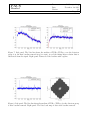
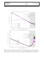
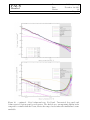
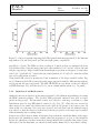
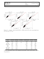
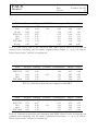
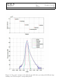
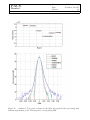
The results are shown in Figure 10. The shaded area in each figure panel highlights the range
of angular scales for which the simulations do not accurately reproduce real PACS data. These
scales typically corresponds to the size of a few instrument beams and below. We strongly
advise against drawing conclusions on the performance of the map-making codes
based on the power spectrum behavior at these angular scales.
At scales larger than the beam, for all considered cases (bright and faint background, blue and
red band) all the mappers appear to reproduce equally well the power spectrum of the truth
map. The only exception appears to be MADmap for the faint background case, both in the
blue and red band, where a slight loss of power at relatively large angular scales is found. The
HPF case is included as a reference and is a clear outliers in all the plots. This is due to the
fact that HPF maps are background-subtracted, thus contain little power on scales larger than
the beam.
PACS
Herschel
Document:
Date:
Version:
PACS-mapmaking
November 1st 2013
1.0
Page 29
Figure 10: Bright background case. Blue band. Uncorrected (top panel) and beam-corrected
(bottom panel) power spectra. The shaded area, encompassing angular scales comparable or
smaller than the beam, denotes the range of scales where the simulations become unreliable.
PACS
Herschel
Document:
Date:
Version:
PACS-mapmaking
November 1st 2013
1.0
Page 30
Figure 10: - continued - Bright background case. Red band. Uncorrected (top panel) and
beam-corrected (bottom panel) power spectra. The shaded area, encompassing angular scales
comparable or smaller than the beam, denotes the range of scales where the simulations become
unreliable.
PACS
Herschel
Document:
Date:
Version:
PACS-mapmaking
November 1st 2013
1.0
Page 31
Figure 10: - continued - Faint background case. Blue band. Uncorrected (top panel) and
beam-corrected (bottom panel) power spectra. The shaded area, encompassing angular scales
comparable or smaller than the beam, denotes the range of scales where the simulations become
unreliable.
PACS
Herschel
Document:
Date:
Version:
PACS-mapmaking
November 1st 2013
1.0
Page 32
Figure 10: - continued - Faint background case. Red band. Uncorrected (top panel) and
beam-corrected (bottom panel) power spectra. The shaded area, encompassing angular scales
comparable or smaller than the beam, denotes the range of scales where the simulations become
unreliable.
PACS
Herschel
5.2
Document:
Date:
Version:
PACS-mapmaking
November 1st 2013
1.0
Page 33
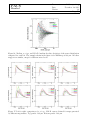
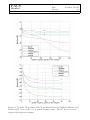
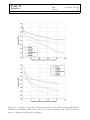
Difference matrix
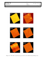
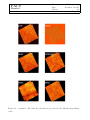
This metric consists in subtracting, from each map reprocessed by the different map-making
codes, a truth reference map. For the reference maps, only the simulated data were used. As in
Section 5.1, we made use of version 3 of the reprojected hybrid simulations, both for the faint
and bright case (more details in Section 3.1). Prior to taking the difference, each map - both
reprocessed and reference ones - was trimmed at the edges to avoid possible artifacts.
To evaluate the result, three quantities were considered:
1. pixel-to-pixel scatter plots of (S - Strue ) vs. Strue , where S is the flux in a given pixel;
2. slopes of the scatter plots;
3. slope-corrected standard deviations (hereafter stdev) of (S - Strue ).
The results are illustrated in Figure 11, 12 and 13 and in Table 3. The slopes in the difference map scatter plots indicate that there is a gain in the flux calibration which is corrected
differently by the map makers. In particular:
• JScanam: its scatter plot is the flattest in all cases (faint/bright, red/blue);
• MADmap: presents a significant slope for the faint background case, both in the blue
and red band;
• Scanamorphos: shows a slight slope which changes from a correlation (red) to an anticorrelation (blue) bahaviour.
The slope/gain corrected stdev of (S-Strue ) gives the high-frequency (pixel to pixel) noise. In
particular:
• faint background, red/blue: the highest stdev is for MADmap. Scanamorphos and
Unimap show the lowest "pixel-to-pixel" noise. Trends are similar for the red and blue
bands;
• bright background, red/blue: the stdev of Tamasis in the red band is the highest. Scanamorphos, Unimap and JScanam show equally low slope-corrected stdev.
5.3
Point-source photometry
One of the most important metrics of the codes benchmarking is point-source photometry.
Goal of this test is to check the quality of the flux ectracted from the reprocessed maps, taking
as a reference the flux estimated from the HPF maps. For this purpose, two flux ranges were
considered, one for bright sources (∼ 0.3 - 50 Jy) and one for faint sources (∼ 0.001 - 0.1 Jy).
PACS
Herschel
Document:
Date:
Version:
PACS-mapmaking
November 1st 2013
1.0
Page 34
Figure 11: Faint blue (70 µm) simulations. Right top corner: truth reference map. All other
panels: difference maps. The quantity shown is: Diff - median(Diff). All the maps are on the
same scale.
PACS
Herschel
Document:
Date:
Version:
PACS-mapmaking
November 1st 2013
1.0
Page 35
Figure 11: - continued - Bright blue (70 µm) simulations. Right top corner: truth reference
map. All other panels: difference maps. The quantity shown is: Diff - median(Diff). All the
maps are on the same scale.
PACS
Herschel
Document:
Date:
Version:
PACS-mapmaking
November 1st 2013
1.0
Page 36
Figure 11: - continued - Faint red (160 µm) simulations. Right top corner: truth reference map.
All other panels: difference maps. The quantity shown is: Diff - median(Diff). All the maps
are on the same scale.
PACS
Herschel
Document:
Date:
Version:
PACS-mapmaking
November 1st 2013
1.0
Page 37
Figure 11: - continued - Bright red (160 µm) simulations. Right top corner: truth reference
map. All other panels: difference maps. The quantity shown is: Diff - median(Diff). All the
maps are on the same scale.
PACS
Herschel
Document:
Date:
Version:
PACS-mapmaking
November 1st 2013
1.0
Page 38
Figure 12: Pixel-to-pixel scatter plot of (S - Strue ) vs. Strue for the faint 70 µm case. No offset
correction applied.
PACS
Herschel
Document:
Date:
Version:
PACS-mapmaking
November 1st 2013
1.0
Page 39
Figure 12: - continued - Pixel-to-pixel scatter plot of (S - Strue ) vs. Strue for the bright 70 µm
case. No offset correction applied.
PACS
Herschel
Document:
Date:
Version:
PACS-mapmaking
November 1st 2013
1.0
Page 40
Figure 12: - continued - Pixel-to-pixel scatter plot of (S - Strue ) vs. Strue for the faint 160 µm
case. No offset correction applied.
PACS
Herschel
Document:
Date:
Version:
PACS-mapmaking
November 1st 2013
1.0
Page 41
Figure 12: - continued - Pixel-to-pixel scatter plot of (S - Strue ) vs. Strue for the bright 160 µm
case. No offset correction applied.
Document:
Date:
Version:
PACS
Herschel
PACS-mapmaking
November 1st 2013
1.0
Page 42
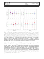
Figure 13: Slope-corrected values of the standard deviation of (S - Strue ) for the faint red/blue
case (left panel) and bright red/blue case (right panel).
MADmap
Tamasis
Scanamorphos
JScanam
Unimap
Faint
red
-0.58
-0.06
0.05
-0.00
-0.03
blue
-0.66
-0.08
-0.02
0.00
-0.10
Bright
red
-0.02
-0.07
0.06
-0.00
-0.01
blue
-0.15
-0.07
-0.03
0.00
-0.08
Table 3: Summary of the slopes obtained, for all the mappers and cases (faint/bright, red/blue),
from the (S – Strue ) vs Strue scatter plots. No errors are quoted.
5.3.1
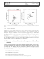
Bright sources (0.3 - 50 Jy)
In this case, the test was done using the Rosette field, i.e. an active star forming region known
to contain at least 100 sources with fluxes ranging from 0.3 to 50 Jy (8). Aperture photometry
at 70 and 160 µm, was performed for each source following these steps:
1. doing a 2D-gaussian fitting at the reference coordinates of the source provided in (8);
2. using the centroid coordinates resulting from the fit for centering the source aperture;
3. using 6" and 12" aperture radii for, respectively, the blue and red band;
4. using 25" and 35" sky apertures around the source for, respectively, the blue and red
band;
5. estimating the photometric errors by placing apertures on empty regions around the
source.
The extracted fluxes were then compared to the reference flux values obtained from the HPF
maps, and the ratio between the two was computed. Additional aperture photometric measurements were done by adopting larger apertures with respect to the standard ones, i.e. 10" and
PACS
Herschel
Document:
Date:
Version:
PACS-mapmaking
November 1st 2013
1.0
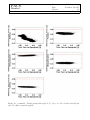
Page 43
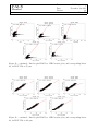
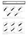
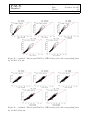
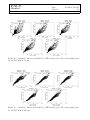
Figure 14: Top panels: photometric measurements in the Rosette field at 70 µm. Left panel:
6" aperture radius. Right panel: results for 10" aperture radius. For each mapper, the average
ratio between the source flux exctracted from the reprocessed map and the reference flux in the
HPF map is plotted. Along the x-axis, from left to right: 1. Scanamorphos, 2. JScanam, 3.
Unimap, 4. Tamasis, 5. MADmap. Bottom panels: photometric measurements in the Rosette
field at 160 µm. Left panel: 12" aperture radius. Right panel: results for 20" aperture radius.
Along the x-axis, from left to right: 1. Scanamorphos, 2. JScanam, 3. Unimap, 4. Tamasis, 5.
MADmap, 6. SANEPIC. The blue dots refer to the case when the outliers are removed from
the sample, while the red dots represent the results for the ensemble of the sources.
20" for the blue and red band, respectively. This operation allowed us to investigate possible
PSF distortion effects in the maps processed by the different codes. The results are shown
in Figure 14 and in Table 4 and 5. All mappers provide accurate photometric measurements
in the considered flux range. In particular, when the outliers are excluded from a statistical
evaluation of the results, they all retrieve fluxes within 5%-10% from the reference values obtained from HPF maps. Moreover, when the recommended aperture radii (6" and 10" for the
blue, red band, respectively) are used and the outliers are rejected, JScanam and MADmap in
the blue band, and JScanam, Scanamorphos, Unimap and MADmap in the red band, retrieve
the best photometric results. In the red band, SANEPIC is an outlier, with recovered fluxes
typically 20% higher than the HPF values.
Document:
Date:
Version:
PACS
Herschel
R(")
6
10
Scanamorphos JScanam
Unimap
Tamasis
1.04±0.09
1.00±0.06 1.04±0.06 1.01±0.08
1.00±0.09
0.98±0.08 1.00±0.09 1.00±0.09
PACS-mapmaking
November 1st 2013
1.0
Page 44
MADmap
1.03±0.05
1.00±0.07
Table 4: Photometric measurements in the Rosette field at 70 µm. Shown in the table are the
ratios between the reference HPF flux values and the fluxes extracted from the data processed
by the mappers.
R(")
12
20
Scanamorphos JScanam
0.97±0.12
1.01±0.12
0.96±0.13
1.01±0.15
Unimap
0.95±0.12
0.97±0.15
Tamasis
1.08±0.16
1.08±0.14
MADmap
0.96±0.104
0.98±0.15
SANEPIC
1.19±0.16
1.15±0.16
Table 5: Photometric measurements in the Rosette field at 160 µm. Shown in the table are the
ratios between the reference HPF flux values and the fluxes extracted from the data processed
by the mappers.
5.3.2
Faint sources (0.001 - 0.1 Jy)
To evaluate the quality of the photometry in the faint-end regime, the PEP Abell 370 field was
used and the following pieces of analysis were carried out:
1. extraction of observed Point Spread Functions (PSFs), using the Starfinder code (6),
following the same procedure as for the PACS Evolutionary Probe (PEP) survey;
2. injection of artificial sources into the science maps, using the observed PSF as object profile, and adopting number counts consistent with deep extragalactic observations. Sources
are injected down to flux limits ∼ 10-20 times deeper than the observed flux thresholds;
3. extraction of sources from the modified science maps (i.e. those including artificial
sources), using Starfinder, tuned as for the PEP survey;
4. derivation of σ, s.i.q.r (semi-interquartile range), MAD of the in/out flux comparison,
after correcting for possible flux trends in the in/out ratio (due to flux boosting at the
faint level in the Starfinder source extraction process, see PEP documentation);
5. extraction of catalogs from original science maps (i.e. extraction of potentially real
sources), and comparison with the PEP official HPF-based blind catalogs.
Each step of analysis is described below.
5.3.3
Extraction of observed PSFs
The PSFs were extracted using Starfinder, piling up the brightest and most isolated point-like
sources in the field. Each PSF (i.e. for each mapper/band combination) is obtained stacking
PACS
Herschel
Document:
Date:
Version:
PACS-mapmaking
November 1st 2013
1.0
Page 45
Figure 15: Curves of growth comparing the PSFs obtained from maps generated by the different
map-makers: 100 µm (left panel) and 160 µm (right panel), respectively.
typically 4-5 objects. The PSFs are cut to a radius of 15 pixels as they are dominated by noise
beyond this radius. Using the maps pixel scale, this translates to 18" and 36" radii at 100 and
160 µm, respectively. Maps obtained with Scanamorphos represent an exception, because their
scale is 1.0 "/pixel and 2.0 "/pixel in the two bands (instead of 1.2" and 2.4"), therefore in this
case an 18 pixel radius was used.
Using these PSFs, curves of growth were built, normalized to the larger available radius. Figure 15 illustrates the PSFs obtained from the maps generated with the different map-makers,
at 100 µm and 160 µm, respectively. The PEP HPF PSFs are not shwon, as they are affected
by HPF flux losses (23), and they need to be cut at a much smaller radius (e.g. 5-6 pixels).
5.3.4
Injection of artificial sources
Artificial sources were injected on the maps generated by the different map-making codes using
the IRAF artdata package. The observed PSFs previously extracted were used as source
profile in this process. Ten thousand sources were added to each map, according to a flux
distribution given by deep FIR number counts (1), (2), (10), (11). Since the area covered by
these maps is very small, the 10000 sources were split in 500 groups of 20 sources each. In
other words, for each map 500 copies were created, and each time only 20 artificial sources
were added, so that the latter are well isolated and the properties of the maps can be studied
without incurring into crowding issues.
Sources were added down to fluxes 10-20 times deeper than the actual flux limits of the maps.
In this way the simulation is more realistic than just stopping at or close to the threshold.
In fact the extraction of sources from these images includes the possibility that faint objects,
effectively below the flux limit, are extracted with brighter fluxes, due to noise flux boosting.
Document:
Date:
Version:
PACS
Herschel
5.3.5
PACS-mapmaking
November 1st 2013
1.0
Page 46
Extraction of sources
Source extraction was performed with Starfinder, using the same configuration/scheme adopted
in the official PEP blind source extraction.
A PSF cut at 6 pixels was used. This conservative cut is necessary to avoid the outer part of the
PSF, which can be rather noisy. Fluxes were then corrected to the 15 pixels radius (adopted
as input) using the c.o.g. of each specific PSF. Furthermore, fluxes were aperture-corrected
using the Enclosed Energy Function (EEF) described in PICC-ME-TN-037 (see Table 15, (19)).
Although this might not be an optimal choice (because the Mars and Vesta observations used in
that case were reduced via HPF, while here we are using different mappers), it likely represents
a good approximation.
Extracted sources/fluxes were then matched to the catalogs of input artificial sources by means
of a simple closest-neighbor algorithm, using a 2.0" maximum matching radius at 100 µm and
3.0" at 160 µm. The comparison between input and output fluxes shows an agreement of the
order of 5-10% for all the mappers, with the only exception of SANEPIC.
5.3.6
Statistics of the output vs. input fluxes
The input and output fluxes are compared by plotting the quantity:
(S(out) − S(in))/S(out)
(4)
vs. S(out) for each mapper at each band. It is worth to emphasize that we are working in
S(out) space, rather than in S(in), as often is done. This is because in the real world, the
quantity S(in) is not known, and one has to stick to S(out) only. Therefore these simulations
provide noise curves to be applied directly to observed quantities without the need of further
assumptions.
For faint fluxes, Starfinder produces a boosted median flux, with respect to the input fluxes.
This is a known effect and it is due to the fact that very faint objects can be extracted with
fluxes significantly higher that their "true" (injected) fluxes, and thus be kept with S(out)
larger than the 3 σ noise threshold, even if in principle they were not supposed to be detected,
because too faint. This effect can happen in the real world as well, and can only be seen in
simulations that include very faint artificial sources as in the present case. Simulations limited
to ∼ 3σ fluxes do not show this effect. When needed, possible trends of (S(out)−S(in))/S(out)
as a function of S(out) were corrected, on the basis of the simulations themselves. See the PEP
global data release documentation for more information about this issue.
The in/out flux comparison is split into flux bins and then the median, σ, s.i.q.r (semiinterquartile range), and M.A.D. (median absolute deviation) of the source distribution in this
plane are computed for each bin. σ is heavily affected by flux-boosted sources, while s.i.q.r.
and M.A.D. are better representantions of the noise properties, as they exclude "outliers". As
a result, few map-makers produce noise levels very similar to the official PEP HPF-based maps
(see Figure 16 and 17).
PACS
Herschel
Document:
Date:
Version:
PACS-mapmaking
November 1st 2013
1.0
Page 47
Figure 16: Median, σ, s.i.q.r, and M.A.D. (median absolute deviation) of the source distribution
computed for each bin. The example shown in the figure is for MADmap at 100 µm. All other
mappers are similar, except for different noise levels.
Figure 17: Left to right: comparison of σ, s.i.q.r., M.A.D. curves obtained for maps generated
by different map-makers. Top panels: 100 µm. Bottom panels: 160 µm.
PACS
Herschel
Document:
Date:
Version:
PACS-mapmaking
November 1st 2013
1.0
Page 48
Figure 18: Comparison of SANEPIC- and Unimap-based 100 mum fluxes to HPF-based PEP
fluxes.
5.3.7
Catalog extraction
Starfinder was also ran on the original map, in order to extract the fluxes of real sources. The
Starfinder configuration adopted in this case is identical to the one used when working on
simulations. Likewise, the PSF cut used in the extraction is again at 6 pixel, which is then
properly corrected for aperture losses using a combination of PSF curves of growth and the
Mars EEF.
All map-makers recover the PEP HPF-based official fluxes within 5-10% at most (see Figure 18
and 19). Differences might be due to the adopted EEF. SANEPIC represents a catastrophic
exception, having a factor ∼6 of flux excess (to be understood).
5.4
Extended emission photometry and comparison with ancillary
data sets
To check the overall reliability of the extended emission photometry in the processed maps,
we performed comparison with ancillary data, in particular IRAS (100 µm) and Spitzer/MIPS
(70 and 160 µm). We emphasize that these comparisons are affected by several caveats that
the user should keep in mind while reading Section 5.4.1 and 5.4.2. A non-comphrensive list of
these limitations includes:
• uncertainties in beam convolutions;
• uncertainties in color corrections;
• uncertanties associated with wavelength scaling;
• uncertainties associated with flux non-linearity effects, if applicable;
PACS
Herschel
Document:
Date:
Version:
PACS-mapmaking
November 1st 2013
1.0
Page 49
Figure 19: Comparison of Unimap-based 160 µm fluxes to HPF-based PEP fluxes.
5.4.1
Comparison with IRAS data
For the purpose of comparing PACS and IRAS data, instead of the original ISSA plates,
the Improved Reprocessing of the IRAS Survey (IRIS, (15)) data were used. The advantage
of the IRIS over the IRAS data is that their absolute zero level is estimated from DIRBE
measurements, yet at no cost of decrease in angular resolution. In addition, they provide an
improved zodiacal light subtraction and destriping of the data. The comparison was performed
at 100 µm, where the IRIS angular resolution is 4.3’. For this metric, only one data set was
suitable from the list in Table 1, namely M31, i.e. a nearby galaxies which is fully resolved
by PACS and sufficiently extended for IRAS to provide enough pixels to make the comparison
meaningful. The remaining fields were rejected either because the emission is too faint (e.g.
Atlas) or there are insufficient pixels at IRAS resolution.
This test was carried out using the same approach discussed in PICC-NHSC-TN-029 (21), that
is:
1. extracting a common region from PACS and IRIS data;
2. putting the PACS and IRIS data in the same units;
3. applying color corrections;
4. convolving PACS data to IRIS resolution;
5. rebinning the convolved PACS data on the IRIS grid;
6. generating scatter plots of the PACS vs. IRIS data sets;
7. fitting the obtained distribution and deriving offset and gain;
PACS
Herschel
Document:
Date:
Version:
PACS-mapmaking
November 1st 2013
1.0
Page 50
8. evaluating the results in the light of possible beam effects.
Below we discuss more in detail the crucial steps of the anlysis.
Unit conversion: since the PACS units are Jy/pixel and the IRIS units are MJy/sr, we converted the PACS maps into surface brightness units. Taking into account the pixel size of the
M31 and NGC 6946 PACS data sets, the conversion factor amounts to 4154.80. Note that the
Tamasis units are already MJy/sr.
Color corrections and wavelength scaling: to compare data produced by two different
instruments, one has to apply a color-correction to both instruments and then a wavelength
scaling to one of the two.
The first correction, which we denote cc, allows the convertion of the the monochromatic flux
density measured by each instrument at the reference wavelength to the true source Spectral
Energy Distribution (SED) flux density. This correction is always necessary, since every instrument quotes the measured flux under a fixed assumption for the input energy distribution
of the source. For both PACS and IRIS, the adopted convention is that the flux scales as
follows an exponential, that is: flux density, Fν , scales with frequency ν as Fν ∝ ν −1 . The
specific corrections to apply depend, as well as on the instrument convention for the input
energy distribution, on the details of the SED of the source and on the wavelength response of
the system. Here, we assumed an ISM SED and adopted the PACS and IRIS color corrections
provided in PICC-NHSC-TN-029. The color-corrected PACS and IRIS data can be expressed
as:
mapP ACS = mapP ACS /ccP ACS
mapIRIS = mapIRIS /ccIRIS
(5)
(6)
The second correction brings the monochromatic color-corrected flux at the reference wavelength of one instrument to the reference wavelength of the other instrument. If the reference
wavelength for the two instruments is the same, as in this case, no correction is needed.
Convolution: the high angular resolution PACS data were convolved to the lower IRIS angular resolution by approximating the IRIS beam with a circular gaussian kernel, normalized to
unity to 7.5’ radius. This step was carried out using the IDL routines PSF_GAUSSIAN and
CONVOL.
Alignining and rebinning: all the PACS and IRIS maps were rebinned onto a common grid.
Non-common pixels are set to NaN values. The reprojection is performed with the IDL routine
HASTROM. Possible astrometric offsets were searched for using peaks of emission.
Scatter plots and fitting: the scatter plots were generated by plotting the pixel distribution
of one data set (e.g PACS) with respect to the corresponding pixel distribution for the other
Document:
Date:
Version:
PACS
Herschel
Field
M31
Scanamorphos
1.07
JScanam
1.02
Unimap
1.03
Tamasis
1.02
MADmap
1.28
PACS-mapmaking
November 1st 2013
1.0
Page 51
SANEPIC
0.99
Table 6: Gain factors derived by comparing the PACS M31 data set reprocessed by the various
map-making codes with the IRIS data.
instrument(e.g. IRIS). The distributions were binned and the mean value computed for every
bin. The binned distributions were fitted with a linear function of the form:
mapP ACS = A × mapIRIS + B
(7)
where A represents the slope or gain factor, and B the offset. Noteworthy, for a given data set,
the offset will vary from code to code: since PACS did not perform absolute measurements over
the course of the mission, so the zero level retrieved by the mappers is arbitrary. The results
are shown in Figure 20 and Table 6. There is generally a good agreement with IRIS fluxes for
all the mappers except for MADmap. We believe the large gain factor is the result of a sloping
background from incorrect drift removal.
Beam effect: the major caveat of this comparison is the significant difference in angular
resolution between PACS and IRIS. A priori, both source confusion and beam convolution
provide plenty of pitfalls. This problem was tackled by attempting to generate an optimal
convolution beam. This was done by adopting as a circular gaussian kernel as a first guess and
then by determining the position offset and the FWHM of the Gaussian by means of a grid of
offsets and FWHM values. The results of this analysis are not given in this report as this is
still work in progress.
5.4.2
Comparison with Spitzer/MIPS data
The test consists in comparing a sub-sample of reprocessed 70 and 160 µm PACS maps with
the corresponding MIPS archival data. At these wavelengths, MIPS has an angular resolution
of 19" and 40", respectively. The list of data sets used for this metric is provided in Table 7.
Note that data selection was carried out with the purpose of covering as wide a parameters
space as possible. Table 7 shows that the comparison includes both galactic and extragalactic
fields, and both the faint and bright-end in surface brightness. The table also indicates which
code, for every given data set, took part in the MIPS comparison.
The test was done following a procedure similar to the one adopted for the IRAS case and
along the lines of what is described in PICC-NHSC-TR-034 (22), i.e.:
1. generating MIPS mosaics with the MOPEX package (12);
2. extracting a common region from PACS and MIPS data;
3. putting the PACS and MIPS data in the same units;
PACS
Herschel
Document:
Date:
Version:
PACS-mapmaking
November 1st 2013
1.0
Page 52
Figure 20: Binned scatter plots of the PACS vs. IRIS data for M31 at 100 µm. The PACS
data reprocessed by each of the mappers are shown in the figure. Note that the offset, i.e.
parameter B, has been removed in order to generate the plot.
Source
MIPS pid
Antennae
Crab
IC348
LDN1780
M31
M81
NGC6949
Rosette
32
130
40372/58
40154
99
717
159
58
λ
Scanamorphos JScanam
µm
70, 160
X
X
70
X
X
70
X
X
70, 160
X
X
70, 160
X
X
70, 160
X
X
70, 160
X
X
70
X
X
MADmap
X
X
X
X
X
X
X
X
SANEPIC
X
only 160
Tamasis
Unimap
X
X
X
X
X
X
X
X
X
X
X
X
X
X
X
X
Table 7: MIPS data sets used for the comparison with the PACS reprocessed maps. The
table content is: source name (1st column); MIPS program ID (pid, 2nd column); wavelength at
which MIPS data are available (3rd column); map-making code and availability of corresponding
reprocessed data set (4th to 9th column).
PACS
Herschel
Document:
Date:
Version:
PACS-mapmaking
November 1st 2013
1.0
Page 53
4. applying color corrections and scaling to a common reference wavelength;
5. convolving, at each wavelength, the PACS data to the MIPS angular resolution;
6. aligning and rebinning the convolved PACS data on the MIPS grid;
7. generating scatter plots of the PACS vs MIPS data sets;
8. fitting the obtained distribution and deriving offset and gain;
9. evaluating the results in the light of non-linearity effects affecting the MIPS detector.
In particular:
Unit conversion: since the PACS units are Jy/pixel and the MIPS units are MJy/sr, we
converted the PACS maps into surface brightness units. Taking into account the different pixel
size of the PACS data sets, the conversion factors amount to: 10636.3 (Antennae, Crab, NGC
6946) and 4154.80 (LDN 1780, M31, M81, Rosette) at 70 µm; 2659.1 (Antennae, NGC 6946)
and 1038.70 (LDN 1780, M31, M81) at 160 µm. Note that the Tamassis units are already
MJy/sr.
Color corrections and wavelength scaling: as mentioned in Section 5.4.1, the PACS
convention is Fν ∝ ν −1 , while for MIPS, the flux is assumed to scale with frequency according
to a blackbody at 10,000 K. In addition, we also need to bring the PACS and MIPS measured
fluxes at the same reference wavelength, that is the PACS surface brightnesses from 160 µm to
155.9 µm, and from 70 µm to 71.4 µm, i.e. the MIPS reference wavelength at 70 and 160 µm,
respectively.
In order to compute color corrections and wavelength scaling, we assumed a fixed dust temperature for each target in Table 7. In particular, the following temperatures were adopted: 20
K (Antennae, M31, M81, NGC 6946, LDN 1780), 30 K (IC 348, Rosette), 50 K (Crab). Following these assumptions, we then applied the PACS color corrections and wavelength scaling
provided in PICC-ME-TN-038 (see Table 3, 3rd and 4th columns, (20)), and the MIPS color
correctons given in the MIPS Data Handbook (14).
In summary, denoting with cc the color correction as in the previous section, and with lc the
wavelength scaling, and using the formalism introduced in PICC-ME-TN-038, we have:
mapP ACS,155.9µm = mapP ACS,160µm /ccP ACS × lc,160µm→155.9µm
mapP ACS,71.4µm = mapP ACS,70µm /ccP ACS × lc,70µm→71.4µm
(8)
(9)
mapM IP S,155.9µm = mapM IP S,155.9µm /ccM IP S
mapM IP S,71.4µm = mapM IP S,71.4µm /ccM IP S
(10)
(11)
and
Document:
Date:
Version:
PACS
Herschel
PACS-mapmaking
November 1st 2013
1.0
Page 54
Convolution: the high angular resolution PACS data were convolved to the lower MIPS angular resolution using a gaussian kernel with an effective Full-Width-Half-Maximum (FWHMef f )
given by:
F W HM ef f =
q
F W HM 2M IP S − F W HM 2P ACS
(12)
where we adopted FWHMM IP S70 = 19", FWHMM IP S160 =40" and FWHMP ACS70 = 6", FWHMP ACS70
= 11". This operation was done using the IDL routines PSF_GAUSSIAN and CONVOL.
Alignining and rebinning: all the PACS and MIPS maps were rebinned onto a common
grid. Non-common pixels are set to NaN values. The reprojection is performed with the IDL
routine HASTROM.
Scatter plots and fitting: the scatter plots were generated by plotting the pixel distribution
of one data set (e.g PACS) with respect to the corresponding pixel distribution for the other
instrument(e.g. MIPS). The pixel-to-pixe distributions so obtained were fitted with a linear
function of the form:
mapP ACS = A × mapM IP S + B
(13)
where A and B represent, respectively a relative gain and absolute offset. See Section 5.4.1 for
more details.
MIPS flux non-linearity: The MIPS 70 and 160 µm arrays are gallium-doped germanium
(Ge:Ga) photoconductor detector. These types of arrays are characterized by a relatively
low absorption coefficient (2 cm-1) and therefore are usually very bulky (0.1-2 mm). This
large physical size has important consequences on the detectors performance, which typically
exhibit a variety of non-linear behaviours. The MIPS 70 µm array is linear only below ∼ 1
Jy, roughly corresponding to a surface brightness threshold of ∼ 100 MJy/sr. For the 160
µm detector, non-linearity effects manifest ∼ 2 Jy, which correspond to ∼ 50 MJy/sr. In the
light of these considerations, we adopted a conservative approach and applied the linear fit, i.e.
Equation (13), to both the original scatter plots distributions and the distributions obtained
by truncating the dynamic range to, respectively, 100 MJy/sr at 70 µm and 50 MJy/sr at 160
µm.
The results of the analysis are provided in Figure 21 and in Table 8 to 11. In the interest of
space, the scatter plots are shown for the original distributions only, while the gain factors are
provided for both the original and truncated distributions. The agreement between the PACS
reprocessed data and the MIPS data in the surface brightness linear regime is typically within
∼10 - 40 %. Noticeable departures are, however, found, such as SANEPIC at 70 µm for the
Crab, and MADmap at 160 µm for both the Antennae and NGC 6946. For IC 348 and LDN
1780 at 70 µm, the χ2 of the fits are unusually high for all the mappers. In these cases, an
analysis of the MIPS data evidences the presence of severe stripes which significantly affect the
quality of the fits.
PACS
Herschel
Document:
Date:
Version:
PACS-mapmaking
November 1st 2013
1.0
Page 55
Figure 21: Pixel-to-pixel PACS vs. MIPS scatter plots, and corresponding linear fit, for the
Antennae data set at 70 µm.
Figure 21: - continued - Pixel-to-pixel PACS vs. MIPS scatter plots, and corresponding linear
fit, for the Antennae data set at 160 µm.
PACS
Herschel
Document:
Date:
Version:
PACS-mapmaking
November 1st 2013
1.0
Page 56
Figure 21: - continued - Pixel-to-pixel PACS vs. MIPS scatter plots, and corresponding linear
fit, for the Crab data set at 70 µm.
Figure 21: - continued - Pixel-to-pixel PACS vs. MIPS scatter plots, and corresponding linear
fit, for IC348 at 70 µm.
PACS
Herschel
Document:
Date:
Version:
PACS-mapmaking
November 1st 2013
1.0
Page 57
Figure 21: - continued - Pixel-to-pixel PACS vs. MIPS scatter plots, and corresponding linear
fit, for LDN 1780 at 70 µm.
Figure 21: - continued - Pixel-to-pixel PACS vs. MIPS scatter plots, and corresponding linear
fit, for LDN 1780 at 160 µm.
PACS
Herschel
Document:
Date:
Version:
PACS-mapmaking
November 1st 2013
1.0
Page 58
Figure 21: - continued - Pixel-to-pixel PACS vs. MIPS scatter plots, and corresponding linear
fit, for M31 at 70 µm.
Figure 21: - continued - Pixel-to-pixel PACS vs. MIPS scatter plots, and corresponding linear
fit, for M31 at 160 µm.
PACS
Herschel
Document:
Date:
Version:
PACS-mapmaking
November 1st 2013
1.0
Page 59
Figure 21: - continued - Pixel-to-pixel PACS vs. MIPS scatter plots, and corresponding linear
fit, for M81 at 70 µm.
Figure 21: - continued - Pixel-to-pixel PACS vs. MIPS scatter plots, and corresponding linear
fit, for M81 at 160 µm.
PACS
Herschel
Document:
Date:
Version:
PACS-mapmaking
November 1st 2013
1.0
Page 60
Figure 21: - continued - Pixel-to-pixel PACS vs. MIPS scatter plots, and corresponding linear
fit, for NGC 6946 at 70 µm.
Figure 21: - continued - Pixel-to-pixel PACS vs. MIPS scatter plots, and corresponding linear
fit, for NGC 6946 at 160 µm.
Document:
Date:
Version:
PACS
Herschel
PACS-mapmaking
November 1st 2013
1.0
Page 61
Figure 21: - continued - Pixel-to-pixel PACS vs. MIPS scatter plots, and corresponding linear
fit, for Rosette at 70 µm.
Field
Antennae
Crab
IC 348
LDN 1780
M31
M81
NGC 6946
Rosette
JScanam
1.61
1.28
0.95
2.34∗
1.08
1.13
2.31
0.66
MADmap
2.20
1.24
0.85
3.18∗
1.20
1.14
2.09
0.98
SANEPIC
—
2.56
—
—
—
—
—
—
Scanamorphos
1.56
1.24
1.54
2.18∗
1.02
1.12
2.06
1.03
Tamasis
1.59
1.26
1.54
1.97∗
1.04
1.13
2.10
1.07
Unimap
1.58
1.25
1.48
2.11∗
0.99
1.08
2.08
1.04
Table 8: Gain factors from 70 µm comparison with MIPS. Values denoted with
low-quality fits.
∗
indicate
Document:
Date:
Version:
PACS
Herschel
Field
Antennae
Crab
IC 348
LDN 1780
M31
M81
NGC 6946
Rosette
JScanam
1.11
0.98
-0.40∗
-0.73∗
1.36
1.38
1.48
-0.36∗
MADmap
1.77
0.94
-1.06∗
-0.61∗
1.31
1.35
1.39
0.88∗
SANEPIC
—
1.44
—
—
—
—
—
—
Scanamorphos
1.10
0.92
1.16
-0.52∗
1.33
1.35
1.38
0.97
PACS-mapmaking
November 1st 2013
1.0
Page 62
Tamasis
1.10
0.94
0.65∗
-0.46∗
1.33
1.36
1.39
0.99
Unimap
1.10
0.94
1.07
-0.50∗
1.31
1.38
1.42
0.91∗
Table 9: Gain factors from 70 µm comparison with MIPS. Quoted values are from the fits
obtained from considering only the surface brightness linear regime, i.e. up to 100 MJy/sr.
Values denoted with ∗ indicate low-quality fits.
Field
Antennae
LDN 1780
M31
M81
NGC 6946
JScanam
1.32
0.95
0.89
1.00
1.22
MADmap
3.62
0.61
1.01
1.06
1.35
SANEPIC
—
—
0.87
—
—
Scanamorphos
1.41
1.02
1.08
1.07
1.35
Tamasis
1.32
0.87
0.97
0.98
1.26
Unimap
1.40
0.89
0.93
1.02
1.35
Table 10: Gain factors from 160 µm comparison with MIPS.
Field
Antennae
LDN 1780
M31
M81
NGC 6946
JScanam
0.74
0.78
0.96
1.07
0.24
MADmap
2.01
-0.07∗
0.94
1.12
0.48
SANEPIC
—
—
0.81
—
—
Scanamorphos
0.79
0.87
1.03
1.13
0.63
Tamasis
0.72
0.74
0.80
1.02
0.78
Unimap
0.81
0.76
0.88
1.11
0.64
Table 11: Gain factors from 160 µm comparison with MIPS. Quoted values are from the fits
obtained from considering only the surface brightness linear regime, i.e. up to 50 MJy/sr.
Values denoted with ∗ indicate low-quality fits.
PACS
Herschel
Document:
Date:
Version:
PACS-mapmaking
November 1st 2013
1.0
Page 63
Figure 22: The Atlas 70 µm data set processed by the different map-making codes.
PACS
Herschel
5.5
Document:
Date:
Version:
PACS-mapmaking
November 1st 2013
1.0
Page 64
Noise analysis
For this metric we selected the Atlas field, which is a large sky area essentially free of emission
except for a few scattered sources. As a consequence, the map is dominated by the noise and
can be considered a sample of the spatial noise introduced by each map-maker. The Atlas
maps produced by the different mappers are shown in Figure 22. The colorbar is adjusted to
leave out 1% of the samples from both tails of the distribution. The field was observed twice
(i.e. using cross-scans), but the pixels at the coverage boundary have only one observation.
These pixels are affected by a higher noise and should be excluded from the measurements,
together with the pixels containing sources. To this end, the pixels not covered or covered by
only one observation are flagged. Moreover, the sources are detected, using a simple algorithm,
and flagged too. No flagged data will be used in the measurements.
We first computed the image variance and the Probability Density Function (PDF). Prior to
the generation of the PDFs, we subtracted the mean value from each map, in order to remove
the offset.
We then calculated a 1D spectrum, which is obtained as follows. Given a window length denoted
by L, we extracted from the image all the rows. We partitioned each row into blocks of 2L+1
samples with an overlap of L samples. We computed the Discrete Fourier Transform (DFT)
of all the blocks, except for the blocks containing flagged data. The procedure is repeated for
all the columns of the image. Finally, the spectrum is given by the average of the squared
magnitudes of all the DFTs so obtained. The DC is zeroed to get rid of the offset.
Last but not least, we estimated a 2D spectrum, according to the following method. Given a
grid step denoted by G, we covered the image with a grid of rows and columns spaced by G
samples. Next, for each row-column crossing point, we extracted from the image a square block
of 2G + 1 by 2G + 1 samples centered on the crossing. We computed the 2D DFT of all the
blocks, except for the blocks containing flagged data. Finally, the 2D spectrum is obtained as
the average of the squared magnitudes of all the 2D DFTs so obtained. The DC is zeroed to
get rid of the offset.
Figure 23 shows the obtained variances and the PDFs in the blue and red band. In the blue
band, Scanamorphos and Tamasis have the lowest variances, JScanam and MADmap have the
highest, and SANEPIC and Unimap fall in between and have the same variances. Moreover
JScanam and MADmap have wider distributions, while the other four have comparable distributions. The MADmap and JScanam distributions are not symmetric. In the red band,
Scanamorphos has the lowest variances, JScanam and MADmap have the highest and the
other mappers are intermediate cases . In addition, JSscanam and MADmap have again a
wider distribution. All distributions are approximately symmetric.
Figure 24 illustrates the 1D spectra for the two bands. x denotes the half-power frequency
i.e. the frequency with respect to which the power is symmetrically distributed, i.e. half of
it lies on the left and half on the right. In the blue band, we note that all the spectra peak
at low frequencies. At higher frequencies JScanam, SANEPIC, MADmap and Unimap yield
essentially a flat spectrum, although with different amplitudes, and the half-power frequencies
lies in the middle of the spectrum. On the contrary, Scanamorphos and Tamasis performance is
frequency dependent. The noise drops at high frequencies and is shifted towards low frequencies,
as indicated by the location of the half-power frequency. Interestingly, the JScanam spectrum
PACS
Herschel
Document:
Date:
Version:
PACS-mapmaking
November 1st 2013
1.0
Page 65
Figure 22: - continued - The Atlas 160 µm data set processed by the different map-making
codes.
PACS
Herschel
Document:
Date:
Version:
PACS-mapmaking
November 1st 2013
1.0
Page 66
Figure 23: Top panel: variance in the Atlas 70 µm field after processing with different mapmaking codes. Bottom panel: corresponding PDF.
PACS
Herschel
Document:
Date:
Version:
PACS-mapmaking
November 1st 2013
1.0
Page 67
Figure 23: - continued - Top panel: variance in the Atlas 160 µm field after processing with
different map-making codes. Bottom panel: corresponding PDF.
PACS
Herschel
Document:
Date:
Version:
PACS-mapmaking
November 1st 2013
1.0
Page 68
Figure 24: Top panel: 1D spectrum of the 70 µm Atlas field processed with the different codes.
Bottom panel: zoom of the 0 to 50 spatial frequency range. The DC has been zeroed. x
indicates the half-power frequency.
PACS
Herschel
Document:
Date:
Version:
PACS-mapmaking
November 1st 2013
1.0
Page 69
Figure 24: - continued - Top panel: 1D spectrum of the 160 µm Atlas field processed with the
different codes. Bottom panel: zoom of the 0 to 20 spatial frequency range. The DC has been
zeroed. x indicates the half-power frequency.
PACS
Herschel
Document:
Date:
Version:
PACS-mapmaking
November 1st 2013
1.0
Page 70
presents, at various frequencies, characteristic peaks which are not found in the 1D spectra
for the other mappers. In the red band, all the spectra peak at low frequencies and display a
frequency dependent behaviour, with a half-power frequency shifted towards lower frequencies.
JScanam, SANEPIC, MADmap and Unimap have a similar spectrum, albeit at different levels,
while the spectrum of Scanamorphos and Tamasis drops at high frequencies.
Figure 25 shows the 2D spectra. In the blue band, one can see that the map-makers are not
isotropic, meaning that the noise is more pronounced along some directions. In particular the
scan directions clearly have an impact on the spatial spectrum, especially for Tamasis. In the
red band, while SANEPIC and Unimap are essentially isotropic, the other mappers are affected
by the scan directions, although to different extents. Note that the aforementioned noise drop
behavior of Scanamorphos and Tamasis at high frequencies, both in the blue and red band, is
clearly visible in Figure 25.
In conclusions, in the blue band Tamasis and Scanamorphos introduce less noise, although
this is of the correlated type (orange peel), while the other four mappers are characterized by
flat, uncorrelated, white noise (salt and pepper). Moreover the mappers are not isotropic and,
in particular, Tamasis introduces more noise along the scan directions. In the red band all
the mappers introduce correlated noise but again the spectrum of Scanamorphos and Tamasis
drops at high frequencies. The spatial spectrum of SANEPIC and Unimap is almost isotropic
while the others are more affected by the scan directions.
6
Conclusions
In the following we summarize the results obtained from application of the metrics described
in Section 5:
• Power spectrum analysis: at scales larger than a few times the beam, for all considered
cases (bright and faint background, blue and red band) all the mappers reproduce equally
well the power spectrum of the truth map. The only exception appears to be MADmap
for the faint background case, both in the blue and red band, where a slight loss of power
at relatively large angular scales is found;
• Difference matrix: some of the mappers appear to introduce a gain in flux calibration, especially MADmap for faint background data, both in the blue/red bands. On
the contrary, JScanam reconstructed maps show no sign of artificial gains. MADmap
also appears to have the highest high-frequency (i.e. pixel-to-pixel) noise, again in the
faint background case, while Scanamorphos and Unimap have the lowest. For bright
background data, Tamasis seems to be characterized by the highest high-frequency noise,
while Scanamorphos, Unimap and JScanam present equally low noise values;]
• Point-source photometry: bright sources (0.3 - 50 Jy): all mappers provide
accurate photometric measurements in this flux range. In particular, when the outliers are
excluded from a statistical evaluation of the results, they all retrieve fluxes within 5%-10%
from the reference values obtained from HPF maps. Moreover, when the recommended
aperture radii (6" and 10" for the blue, red band, respectively) are used and the outliers
PACS
Herschel
Document:
Date:
Version:
PACS-mapmaking
November 1st 2013
1.0
Page 71
Figure 25: 2D spectrum of the 70 µm Atlas field processed with the different codes. The DC
has been zeroed.
PACS
Herschel
Document:
Date:
Version:
PACS-mapmaking
November 1st 2013
1.0
Page 72
Figure 25: - continued - 2D spectrum of the 160 µm Atlas field processed with the different
codes. The DC has been zeroed.
PACS
Herschel
Document:
Date:
Version:
PACS-mapmaking
November 1st 2013
1.0
Page 73
are rejected, JScanam and MADmap in the blue band, and JScanam, Scanamorphos,
Unimap and MADmap in the red band, retrieve the best photometric results. In the red
band, SANEPIC is an outlier, with recovered fluxes typically 20% higher than the HPF
values;
• Point-source photometry: faint sources (0.001 - 0.1 Jy): in this faint flux regime,
for the blue band the photometric measurements of the different mappers are comparable
to the performance of HPF down to fluxes of the order of 0.003 Jy. Below this threshold,
JScanam appears to provide the largest departures from the HPF fluxes, while Unimap
and Scanamorphos provide the closest. In the red band, the thereshold of comparable
fluxes between the mappers and HPF is an order of magnitude higher with respect to the
blue band, i.e. ∼ 0.03 Jy. Below this threshold, MADmap, JScanam and Scanamorphos
give the noisiest measurements, while Unimap retrieves the closest to HPF values. None
of the codes appear to introduce significant distortions of the PSF;
• Extended emission photometry - IRAS comparison: the comparison between
PACS and IRAS/IRIS data at 100 µm for only one data set (M31) shows that there
is generally a good agreement with IRIS fluxes for all the mappers except for MADmap,
for which the comparison retrieves a gain factor of the order of 30%;
• Extended emission photometry - Spitzer/MIS comparison: the agreement between the PACS reprocessed data and the MIPS data in the surface brightness linear
regime is typically within ∼10 - 40 %. Noticeable departures are, however, found, such
as SANEPIC at 70 µm for the Crab, and MADmap at 160 µm for both the Antennae
and NGC 6946. For IC 348 and LDN 1780 at 70 µm, the χ2 of the fits are unusually high
for all the mappers. In these cases, an analysis of the MIPS data evidences the presence
of severe stripes which significantly affect the quality of the fits;
• Noise analysis: in the blue band Tamasis and Scanamorphos introduce less noise, although this is of the correlated type (orange peel), while the other four mappers are
characterized by flat, uncorrelated, white noise (salt and pepper). Moreover the mappers
do not have an isotropic behaviour and, in particular, Tamasis introduces more noise
along the scan directions. In the red band all the mappers introduce correlated noise but,
as in the blue band, the spectrum of Scanamorphos and Tamasis drops at high frequencies. The spatial spectrum of SANEPIC and Unimap is almost isotropic while the others
are more affected by the scan directions.
References
[1] Berta, S., Magnelli, B., Lutz, D., et al., 2010, A&A, 518, 30
[2] Berta, S., Magnelli, B., Nordon, R., et al., 2011, A&A, 532, 49
[3] Billot, N., et al., 2010, SPIE, 7741, 1
[4] Calabretta, M. R. & Greisen E. W., 2002, A&A, 395, 1077
PACS
Herschel
Document:
Date:
Version:
PACS-mapmaking
November 1st 2013
1.0
Page 74
[5] Cantalupo, C., et al., astro-ph/09061775
[6] Diolaiti, E., Bendinelli, O., Bonaccini, D., et al. 2000, A&AS, 147, 335
[7] Greisen, E. W. & Calabretta, M. R., 2002, A&A, 395, 1061
[8] Hennemann, M., Motte, F., Bontemps, S., et al., 2010, A&A, 518, 84
[9] Herschel Map-Making Workshop, http://herschel.esac.esa.int/2013Mapmaking.shtml
[10] Lutz, D., Poglitsch, A., Altieri, B., et al., 2011, A&A, 532, 90
[11] Magnelli, B., Popesso, P., Berta, S., et al., 2013, A&A, 553, 132
[12] Makovoz, D. & Khan, I., 2005, In ASP Conf. Ser., 132
[13] Meixner, M., Panuzzo, P., Roman-Duval, J. et al., 2013, AJ, 146, 62
[14] MIPS Instrument Handbook, http://irsa.ipac.caltech.edu/data/SPITZER/docs/mips/
mipsinstrumenthandbook/51
[15] Miville-Deschenes, M.-A. & Lagache, G., 2005, ApJS, 157, 302
[16] Patanchon, G., Ade, P. A. R., Bock, J. J., et al., 2008, ApJ, 681, 27
[17] Piazzo, L., Ikhenaode, D., Natoli, P., et al., 2012, "Artifact removal for GLS map makers
by means of post-processing", IEEE Trans. on Image Processing, Vol. 21, Issue 8
[18] Piazzo, L., "Subspace Least Square Approach for Drift Removal with Applications to
Herschel Data", in preparation
[19] PICC-ME-TN-037, http://herschel.esac.esa.int/twiki/pub/Public/PacsCalibrationWeb/
pacs_bolo_fluxcal_report_v1.pdf
[20] PICC-ME-TN-038, http://herschel.esac.esa.int/twiki/pub/Public/PacsCalibrationWeb/
cc_report_v1.pdf
[21] PICC-NHSC-TN-029, https://nhscdmz2.ipac.caltech.edu/pacs/docs/Photometer/
PICC−NHSC−TN-029.pdf
[22] PICC-NHSC-TR-034, https://nhscsci.ipac.caltech.edu/pacs/docs/Photometer/
PICC−NHSC−TR-034.pdf
[23] Popesso, P., Magnelli, B., Buttiglione, S., et al., astro-ph/12114257
[24] Roussel, H. 2012, astro-ph/12052576
[25] Roussel, H. 2012, proceedings of the annual meeting of the SF2A, ed. S. Boissier, P. de
Laverny, N. Nardetto, R. Samadi, D. Valls-Gabaud and H. Wozniak, p. 559-563
[26] Tegmark, M., 1997, ApJ, 480, 87
[27] UniHIPE Web Page, http://herschel.asdc.asi.it/index.php?page=unimap.html
[28] Unimap Web Page, http://w3.uniroma1.it/unimap