Download Lab5 – Quanser Coupled Tanks Modeling and

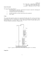
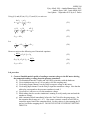
MEEN 364
Vijay Alladi, 2001. Aninda Bhattacharya, 2002.
Andrew Rynn, 2002. Justin Mlcak 2005
Last Update: 3 September 2012 by A.G. Parlos
Lab5 – Quanser Coupled Tanks Modeling and Parameter
Identification
Introduction
A common control problem in petrochemical process industries is the control of liquid levels in storage
tanks, chemical blending and reaction vessels. A typical situation is the one that requires supplying
fluid at a constant rate qi .A reservoir can be used with the dual aim of filtering out any variations in
the upstream flow and ensuring a temporary supply of reactant in case of process failure upstream of
the “hold-up” tank. This may be achieved by a feedback control loop, which maintains a constant level
h of fluid in the tank by controlling the input flow rate qi or the position of a valve in the outlet. Like
the modeling of DC motor, this lab is also a setup of the liquid level system for further experiments.
Objective
•
•
•
To derive the mathematical model which governs the fluid levels in the two-tank system
To determine the numerical parameters in the model. This is called parameter identification.
To calibrate the transducers used in the setup.
Prelab:
The system shown above consists of a tank with a liquid of density ρ . Find out the mass flow rate of
the liquid leaving the system.
1
MEEN 364
Vijay Alladi, 2001. Aninda Bhattacharya, 2002.
Andrew Rynn, 2002. Justin Mlcak 2005
Last Update: 3 September 2012 by A.G. Parlos
System Description
The experimental setup consists of
1
Two hold-up tanks, with orifice 1 draining tank 1 into tank 2, and orifice 2 draining tank
2 into the fluid reservoir for the pump.
2
A pump driven by a DC motor to fill tank 1.
3
A pressure transducer to measure the pressure in the second tank.
4
Power supply.
Tanks
The coupled tank apparatus consists of two transparent Plexiglas tubes 32.5 cm long, each with an
inside diameter of 4.5 cm. Deionized water from a reservoir is pumped into the top of tank 1, which
drains through orifice 1 into tank 2 below it. Tank 2 then drains via orifice 2 into the fluid reservoir.
The entire assembly is mounted on a Plexiglas frame.
Figure 3 – Quanser coupled tank system (modified from Quanser User Manual)
Pump Unit
2
MEEN 364
Vijay Alladi, 2001. Aninda Bhattacharya, 2002.
Andrew Rynn, 2002. Justin Mlcak 2005
Last Update: 3 September 2012 by A.G. Parlos
Water is pumped from the reservoir to the first tank by means of a variable speed gear pump driven by
an electric motor. The motor changes speed rapidly in response to changes in input voltage compared
to the time required for the tank levels to change. Therefore motor dynamics will be neglected. In
effect, this means that the motor speed is always proportional to the supply voltage. The flow rate for
the pumping unit is proportional to the input voltage.
qi = kvi
(a)
The maximum voltage that the motor can tolerate is 12 V. However, since the DAQ can only handle
up to 10 V, the voltage supplied to the motor will be limited by a saturation block.
Instrumentation
Pressure transducer
The pressure transducers are located at the bottom of tanks 1 and 2. Note that in this lab we will only
be reading pressure from tank 2. The pressure transducers give a voltage proportional to the height of
the liquid in the tank.
h2 = k pt v pt
(b)
Signal Conditioning Board
The output of the pressure transducers are filtered and amplified in the signal conditioning board
before they are sent to the DAQ. This processed signal ranges from 0 to 5 V.
NOTE: The pump should not run without water.
Theory
The governing equations of motion can be derived as below.
Applying conservation of mass for tanks 1 and 2
∂h
qi − q12 − A1 1 = 0
∂t
dh
q12 − q e − A2 2 = 0
dt
where qi is the volume inflow rate from the pump to the tank 1,
q12 is the flow rate from tank 1 to tank 2.
q e is the flow rate of fluid coming out from tank2.
A1 and A2 are the cross-sectional areas of tanks 1 and 2, respectively.
h1 and h2 represent the height of liquid in the tanks at any given time.
Applying Bernoulli’s equation:
between points a and b gives,
3
(1)
(2)
MEEN 364
Vijay Alladi, 2001. Aninda Bhattacharya, 2002.
Andrew Rynn, 2002. Justin Mlcak 2005
Last Update: 3 September 2012 by A.G. Parlos
2
2
Va
P V
P
+ a = b + b
ρ
ρ
2
2
between points c and d gives,
2
(3)
2
Vc
P V
P
+ c = d + d
ρ
ρ
2
2
(4)
where
Pa = ρgh1 , Pb = 0, Pc = ρgh2 , Pd = 0
(5)
Va = 0,Vc = 0
The following notation has been used above
V ' s represent the velocities and
P' s represent the pressures.
ρ represents the density of the liquid being used.
Volumetric flow rates can be determined as
q12 = Vb Ab
q e = Vd Ae
(6)
(7)
inserting (6) into (3) and simplifying we get
q12 = Ab 2gh1
(8)
inserting (7) into (4) and simplifying we get
q e = Ae 2gh 2
(9)
The actual flow rates are lesser than the theoretical flow rates, by some factor. So we have
q12 = cd 1 Ab 2 gh1 = c1 h1
(10)
qe = cd 2 Ae 2 gh2 = c 2 h2
(11)
Using (10) and (11) in (1) and (2) we get
qi − c1 h1 − A1
dh1
=0
dt
(12)
4
MEEN 364
Vijay Alladi, 2001. Aninda Bhattacharya, 2002.
Andrew Rynn, 2002. Justin Mlcak 2005
Last Update: 3 September 2012 by A.G. Parlos
c1 h1 − c2 h2 − A2
dh2
=0
dt
(13)
qi = kvi
(14)
The above equation assumes that for our operating conditions the input-output relation of the pump is
linear.
d
At steady state we have
=0
dt
So we have from (12) and (13)
qi 0 = c1 h10
(15)
c1 h10 = c2 h20
⇒ qi 0 = c 2 h20
(16)
Rewriting (15) and (16) we get*
⎛q ⎞
h20 = ⎜⎜ i 0 ⎟⎟
⎝ c2 ⎠
⎛q ⎞
h10 = ⎜⎜ i 0 ⎟⎟
⎝ c1 ⎠
2
(17)
2
(18)
Given h20 , parameters q120 , qe 0 , h10 and qi 0 can be established.
Now let us linearize the non-linear equations that we obtained in (12), (13), (14)
Assuming
h1 = h10 + δ h1 ;
h2 = h20 + δ h2 ;
(19)
qi = qi 0 + δ qi
where
( )0
refers to the equilibrium value.
Using Taylor’s series of expansion we have
⎛ δ h1 ⎞
⎟⎟
h1 = h10 ⎜⎜1 +
2
h
10
⎝
⎠
⎛ δ h2 ⎞
⎟⎟
h2 = h20 ⎜⎜1 +
⎝ 2h20 ⎠
(20)
5
MEEN 364
Vijay Alladi, 2001. Aninda Bhattacharya, 2002.
Andrew Rynn, 2002. Justin Mlcak 2005
Last Update: 3 September 2012 by A.G. Parlos
Using (19) and (20) in (12), (13) and (14) we arrive at
A1
dδ h1
dt
c1δ h1
2 h10
−
+
c1δ h1
2 h10
c 2δ h 2
2 h20
= δ qi
= A2
(21)
dδ h2
(22)
dt
δ qi = kδ vi
(23)
Let
c1
2 h10
= Gv1 ;
c2
2 h20
= Gv2 ;
(24)
Hence we arrive at the following set of linearized equations
dδ h1
A1
+ Gv1δ h1 = δ qi
dt
dδ h2
Gv1δ h1 −Gv2δ h 2 = A2
dt
δ qi = kδ vi
(25)
(26)
(27)
Lab procedure
1. Create a Simulink model capable of sending a constant voltage to the DC motor driving
the pump and reading a voltage from the pressure transducer.
a) Use Simulation Interface Toolkit and LabVIEW to interface with the hardware.
b) Use a simulation step size of 0.01 seconds (a 100 Hz sampling rate).
c) Use Analog Output channel 1 on the DAQ to output a voltage to the motor.
d) Use Analog Input channel 2 on the DAQ to input the transducer voltage. Note that the
white plug corresponds to the pressure transducer in tank 2.
e) Use a numeric indicator to view the transducer voltage.
f) While taking data, be sure the simulation is running to verify steady state and read the
transducer voltage.
g) Add a saturation block immediately before the “Out” block for the pump motor.. Set
the saturation block range as 0 – 4 V. Also create a numeric control in LabVIEW to
control the upper limit of the saturation block. Set this value to 4 when running the VI
and to 0 just before stopping the VI. DO NOT STOP THE VI WITHOUT SETTING
THIS TO 0.
6
MEEN 364
Vijay Alladi, 2001. Aninda Bhattacharya, 2002.
Andrew Rynn, 2002. Justin Mlcak 2005
Last Update: 3 September 2012 by A.G. Parlos
2. Determination of C1 and C2
a) Select five voltages to send to the pump motor as follows:
i. If the coupled tanks system does not settle with the maximum motor voltage,
determine maximum pump motor voltage at which the coupled tanks system
reaches steady state (i.e. does not overflow).
ii. Minimum motor voltage that yields a flow into tank 1. Stop the pump if there is
air in the suction line.
iii. Three additional voltages equally spaced between maximum and minimum
voltages.
b) Send voltages to pump motor in descending order.
c) Allow coupled tanks system to reach steady state (this will likely take 10 – 15 minutes).
d) Record heights of tanks 1 and 2, as well as motor voltage.
e) Estimate the pump flow constant for the Quanser tanks. Use this information to plot
flow rate vs. h11/2 Æ C1 is slope of linear fit with a 0 intercept.
f) Plot flow rate vs. (h2)1/2 Æ C2 is slope of linear fit with a 0 intercept.
3. Calibration of Pressure Transducer
a) Set height of tank 2 to values from 0 – 20 cm in 1 cm increments.
b) Record voltage from pressure transducer.
c) Plot height of tank 2 vs. pressure transducer voltage – determine linear calibration
equation with a non-zero intercept.
4. Estimation of Steady State Gain – plot h2 Vs vin to find an estimate of the steady state
gain of the system, k̂ s .
Issues to be addressed in the report
1. Description of the set up
2. Calibration of the pressure transducer
3. Parameter identification- All the parameters of the system that you had to find
experimentally
4. Include all calibration plots.
Things you have learned in this lab
1
2
3
Modeling of nonlinear systems.
Taylor series and linearization.
Calibration of sensors.
7