Download Chapter 2 Getting Started

Chapter 2
Getting Started
2.1
Introduction
In this tutorial manual, an introduction is given how to work with COHERENS. We present two COHERENS test cases (river and bohai) and show
how to compile the code, run the test case, view the results with various free
software visiualisation tools and show how model setup is arranged and can
be modified.
The objective of this chapter is to give a first introduction to COHERENS
for a beginning user. A more extended description with more technical details about installation and compilation of the code are found in the User
Documentation.
2.1.1
General requirements
We will make the following assumptions on your system and the installation
of COHERENS.
• You use COHERENS V2.4 or higher. Older versions of COHERENS have
a slightly different syntax.
• You have managed to install COHERENS correctly and to set the compiler options correctly in compilers.cmp (see below).
• You have a working installation of netCDF on your computer or work
station. Note that if you install a compiler, you have to do this before
you install netCDF. Otherwise, the netCDF installation will not generate
the correct binary files for your compiler.
15
16
CHAPTER 2. GETTING STARTED
• You have some software for doing post processing. In this manual, we
will use the free software packages NcView, Ferret and Octave. However,
it is very well possible to use other (free or commercial) post-processing
software such as IDL or Matlab, as long as they can read the netCDF
format.
Some other external libraries, which you can use with COHERENS (such
as MPI), will not be used in this introduction. The used software and libraries
can be found at:
• MPI: http://www.mcs.anl.gov/research/projects/mpich2/
• netCDF: http://www.unidata.ucar.edu/software/netcdf/
• NcView: http://meteora.ucsd.edu/~pierce/ncview_home_page.html
• Ferret: http://ferret.wrc.noaa.gov/Ferret/
• Octave: http://www.gnu.org/software/octave
2.1.2
Short Linux introduction
This section will make you familiar with working under Linux. If you are
already familiar with Linux, you can skip this section without problem.
The first thing to do is to open a terminal in which we can execute the
commands we need. Before we continue, there are three important things to
know when working on the Linux command line:
1. Linux commands and file names are case sensitive. Thus Run is not
the same as run.
2. Linux can help you finish commands (especially file names and directories) when you press on the tab key. Try using this as often as possible.
3. In Linux, files and folders are separated by a forward slash (/) not a
backslash (\) that is used in Windows. Using the wrong slash can give
very unexpected results!
The following commands are very useful when working with Linux.
2.1. INTRODUCTION
2.1.2.1
17
getting help
If you do not know which command to use, use apropos. It will tell you
which commands to use. For example, if you want to know how to copy a
file, type
apropos copy
This gives you many results, including the one you need, which is cp. In
order to understand how to use this command, use man. Type
man cp
2.1.2.2
working with files
To see which files are in a directory use ls or ls -l1 . The latter gives more
information. Try them both
ls
ls -l
Aliases for some commands may be defined on your computer. A common
alias is ll which is the same as ls -l. The command for copying a file is
cp sourcefile destination
The command for moving a file
mv sourcefile destination
The command for deleting a file is
rm filetodelete
In case you want to use any of these commands on directories, you must add
-r
rm -r directorytodelete
In order to know how much free space there is on the hard disk, type
df -h
Finally it is important to know that you can use the | symbol to send output from one program to another program. For example, you can use the
command less to view the output of the previous command
df -h | less
Exit less by typing the letter q.
1
note that ‘l’ is the letter l and not the number ‘1’.
18
CHAPTER 2. GETTING STARTED
2.2
2.2.1
Running a test case
Installing a COHERENS test case
First, you will need to go to the directory where the COHERENS source
files are installed. We will assume here that we have them installed on the
directory ∼/V2.5 where ∼ stands for your home directory2 . When installing
a COHERENS test case, such as the river test, we always start by making
a new folder in which the results are placed. In order to do so, type the
following commands
cd
mkdir river
cd river
We follow by making a link to the COHERENS directory, in which the source
code and installation scripts are placed. The name of the link must be
COHERENS. We can make the link by typing the following command
ln -s ../V2.5/ COHERENS
Here, the two arguments are first the location to which the link points and
secondly the name of the link. In this command, the two dots (..) are used
to refer to the directory that is above the current directory. In case the
COHERENS source files are located in another directory, you must adapt
the first argument (../V2.5) such that it is the location of the directory
containing your COHERENS files.
The first test case that we are going to do is called river. It describes the
evolution of an estuarine salinity front advected by a tidal current and the corresponding estuarine circulation in an open non-rotating channel (as described in the User Documentation). We run the installation script install test
in the COHERENS directory, which copies the necessary files to our directory
COHERENS/install_test -t river
In this command, the argument of the script is the name of the test cases3 .
There are many test cases delivered with COHERENS. Their model setups
can be found in the directory COHERENS/setup.
In order to examine the files that are generated, we use the command ls.
Type
2
The examples below can be run in the same way with other versions of COHERENS
as long as they are not older than 2.4.
3
The -t option is new from COHERENS V2.4 on. In older versions, this option must
not be used.
2.2. RUNNING A TEST CASE
19
ls
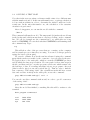
Now, you should see the following output
BCOMPS
BSOURCE
cifruns
COHERENS
coherensflags.cmp
COMPS
con_sub_river
DATA
deffigs.txt
defposts
defruns
files.vis
Makefile
postparsA
postparsB
postparsC
postparsD
river.txt
Run
Run_hpd_par
Run_hpd_ser
Run_vic
SCOMPS
SCR
SETUP
SOURCE
SSOURCE
Usrdef_Harmonic_Analysis.f90
Usrdef_Model.f90
Usrdef_Output.f90
Usrdef_Time_Series.f90
The files have different meanings. They are not all necessary for our purposes.
We will now examine the most important of these files.
The names in capitals are symbolic links to important locations for COHERENS. For example, the link SOURCE points to the FORTRAN source
files of the model. The link COMPS points to the files needed for the compilation. The model setup is given in the four files whose name starts with Usrdef . For our purposes, the two most important ones are Usrdef Model.f90,
which contains the model input and Usrdef Time Series.f90, which contains
information on the data that should be exported as time series. We will
discuss this later in the tutorial.
After installing the test case, we are now ready to compile the model.
This will be explained in the next section.
2.2.2
Compiling COHERENS
Before we compile the model, we have a look at the files that determine
the compilation process. There are three. First there is Makefile, which
contains instructions about the order in which the model is compiled. Second,
there is the file coherensflags.cmp. This file contains some statements, which
determine which options are used in the compilation of the model. Thus you
can make the program a little bit different by changing the options in this
file. We will edit this file. An easy to use text editor with a graphical user
interface in Linux is called gedit. Open the file by typing
gedit coherensflags.cmp
Note that, if gedit is not installed on your system, or if you prefer other
text editors, such as vi, nano or emacs, you can of course use these instead
of gedit.
Now, we are going to add two options. Change the line that starts with
CPPDFLAGS = into the following
20
CHAPTER 2. GETTING STARTED
CPPDFLAGS = -DALLOC -DCDF
The meaning of these two switches is the following. The first one (-DALLOC)
changes the location in the memory that is used in COHERENS (more variables are placed on the heap instead of on the stack). The first advantage of
using this option is that there is a much lower risk that the model crashes,
because the amount of memory is too low. The reason is that there is much
more memory available on the heap than on the stack. The second advantage
is that less CPU memory is used by the model. The eventual disadvantage
of using this option is that the model might become slightly slower. The
second option (-DCDF) enables the netCDF module in COHERENS. Without
this option, it is not possible to use netCDF input and output. If you do not
set this option and you are trying to generate netCDF output, COHERENS
will run normally, but the files are not generated! Another option that can
be set in this way and which will not further discussed in this tutorial, is the
enabling of parallel computations by setting the switch (-DMPI).
Further, you need to select the paths of the netCDF installation (usually,
this is in /usr/local). You can do this by removing the comments (indicated
by a hash #) in the lines related to netCDF, and changing (if necessary) the
location of your netCDF files. The result should look something like this
# netCDF directory path
NETCDF_PATH = /usr/local
# netCDF library file
NETCDF_LIB_FILE = netcdf
# netCDF include options
FCIFLAGS_NETCDF = -I$(NETCDF_PATH)/include
# netCDF library options
FLIBS_NETCDF = -L$(NETCDF_PATH)/lib -l$(NETCDF_LIB_FILE)
Now save and close the file. The third file that is important for the course is
compilers.cmp which is located in the folder COHERENS/code/physics/comps
given by the symbolic link COMPS. We will open this file in gedit to see
its contents
gedit COMPS/compilers.cmp
In this file, there is a list of “targets”. Each target defines a set of options
for different compilers. If one these compilers has been installed on your
machine, there is, in principle, no need to change this file. We will use here
2.2. RUNNING A TEST CASE
21
the Intel Fortran compiler (ifort), or the GNU Fortran compiler (gfortran).
We will look up the settings for this compiler in compilers.cmp. In this file,
you should see the following statements (they may be different because of
local settings on your computer)
# Linux gfortran (GNU Fortran)
linux-gfort:
$(MAKE) $(EXEFILE) "FC=gfortran" "FCOPTS= -O3" "FCDEFS=" "FCDEBUG=" \
"CPP=" "CPPF=cpp" "CPPOPTS=-traditional-cpp" "CPPDEFS=$(CPPDFLAGS)"
#Intel fortran compiler v 9 without MPI, dynamically linked
linux-iforts:
$(MAKE) $(EXEFILE) "FC=ifort" "FCOPTS=-cpp1 -i-dynamic" \
"FCDEFS=$(CPPDFLAGS)" "FCDEBUG=" \
"FCIFLAGS_COMP=-Wl,-rpath=/usr/local/intel/lib" \
"CPP=" "CPPF=@cp" "CPPOPTS=" "CPPDEFS="
The first word before the colon (e.g. linux-iforts) is the name of the compiler
setting, also called the “target”. There are two settings for the Intel compiler in this file. linux-iforts is the normal option for using the Intel Fortran
Compiler. This is the recommended setting when performing simulations.
In this tutorial, we will make a few changes in this file in order to speed up
the compilation process. This is done by disabling the optimization that is
performed by the compiler. This optimization takes a lot of time. On our
machine, the compilation with optimization takes about 25 minutes. Without optimization, it takes only one minute. However, the optimized version
executes much faster (up to 5 times faster). Therefore, for real simulations,
one should always use this optimization.
If you are using the gfortran compiler, you can switch of the optimization
by setting (take care with the difference between, the capital O and the
number 0!)
"FCOPTS= -O0"
For the Intel Fortran compiler, you can disable the optimization by setting
"FCDEBUG= -O0"
In order to compile the code, close gedit and type (for gfortran)
make linux-gfort
In order to compile the model using the Intel Compiler, type
22
CHAPTER 2. GETTING STARTED
make linux-iforts
This command will print some information on the screen mainly showing,
which files were compiled. It may also show some warnings or errors. In case,
the compilation was successful, the last output line should be something like
make[1]: Leaving directory ‘/home/coherens/rivertest’
The compilation generated many additional files. Use the command ls in
order to examine the files that are present in the working directory.
We are now ready to run the simulation.
2.2.3
Running COHERENS
In COHERENS, the different runs that are done during a simulation are defined in the file defruns, which is located in the working directory. Open this
file in gedit in order to examine the runs that are being performed
gedit defruns
In this file, all the runs are defined, with the following syntax
Run name,CIF options, CIF file name
Note that the last two inputs (CIF option and CIF file name) are optional,
which means that you can leave them empty. However, you must always put
the two commas on this line. Otherwise, COHERENS will generate an error.
Comments can be set in the defruns file by adding an exclamation mark (!).
There are two options for CIF files. In order to read a CIF file, one must
add the letter R (note that this option is case sensitive). In order to write a
CIF file, one must add the letter W. We will change the defruns file. We do
so by adding W after the first comma on the first two lines and inserting an
exclamation mark at the beginning of the next lines. The result looks like
river0A,W,
river1A,W,
!river0B,,
!river1B,,
!river0C,,
!river1C,,
!river0D,,
!river1D,,
2.2. RUNNING A TEST CASE
23
Note that in the test case river, each run actually exists of two different runs
with the numbers 0 and 1. In the run with number zero, a spin up calculation
is done without salinity in order to determine the initial conditions for the
actual run. In the run with number one, the calculation of the estuarine
circulation is performed.
After closing gedit, we can run the model with the command:
./Run &
This command will run the model. The ampersand (&) makes the model run
in the background, which means that we can keep working on the command
line. We can for example use the command ls to see which files are being
made by COHERENS. We can check whether COHERENS is still running with
the command top. Type:
top
This will show a list of the processes that are occurring on the computer
and how much processor time they are using. You can close this program by
typing the letter q (from quit).
We can also examine how far the run has advanced using the command
grep which searches a text file for the occurrence of a word given by the user.
We apply it here to the runlog file, which is a text file COHERENS produces
and in which the time step is written. We can search for these time steps in
the file, and then send it to another program, called tail which returns only
the last lines of data. For sending information from one program to the next
(this is called a pipe) we use the vertical line (|). Thus in order to find the
last occurrence of the string “2003” (the calculations in this file have a start
date and end date in 2003) in the runlog file, we use the command:
grep 2003 river0A.runlogA | tail -1
You can also use this command without tail, in order to get all occurrences
of the string “2003”:
grep 2003 river0A.runlogA
After the model has finished, something like this will be written to the
terminal
Main program terminated
real
user
sys
0m19.678s
0m18.490s
0m1.154s
24
CHAPTER 2. GETTING STARTED
Let’s have a look at the files that are generated by COHERENS. All these
files have a name that is generated from the name of the run (defined in the
file defruns).
ls river*
This should give the following result
river0A.cifmodA
river0A.inilogA
river0A.runlogA
river0A.timingA
river0A.warlogA
river1A.cifmodA
river1A.inilogA
river1A.runlogA
river1A.timingA
river1A.warlogA
riverA_1.resid3I
riverA_1.resid3N
riverA_1.tsout2I
riverA_1.tsout2N
riverA_1.tsout3I
riverA_1.tsout3N
riverA_2.tsout0A
riverA_2.tsout0I
riverA.2uvobc1U
riverA.modgrdU
riverA.phsicsU
river.txt
These files have the following meanings
• Files ending at .inilogA are the initialization log files. The name of
each subroutine that is called during the initialization is written to this
file. It is mainly important for debugging of a model setup and code
developers.
• Files with suffix .runlogA are log files writing information during the
actual run of the model. This files may become quite large for long
runs. We have already seen it before when we used this file to examine
the progress of the simulations. Otherwise, it is also more important
2.2. RUNNING A TEST CASE
25
for code developers than for model users. However, it sometimes occurs that an error is written to a log file, in addition to the errlog file
discussed below.
• The files ending with .timingA contain information on the time it took
for the model to run. Open the file river0A.timingA in gedit and
examine the results. This file shows how long the simulation took and
it also shows the percentages of the time that different parts of the
calculation took (such as 2D calculation, 3D calculation, input and
output, . . . ).
• Files ending at .warlogA are files with warnings about settings that
were automatically changed by COHERENS. Before the start of the simulations, COHERENS checks whether some parameters in the model
have appropriate values, and if not, COHERENS resets them automatically. When COHERENS changes these values it writes a warning in
this file. It may be useful after each simulation to inspect the .warlogA
files! They can give information on some model settings that were not
intended by the user and they may explain unexpected results in the simulations. Open river0A.warlogA in gedit and examine the warnings.
In this case, there are no important changes made to the model.
• A file that should not be present is the .errlogA file. In this file, error
messages are written and the execution of the program stops. Examples
of this are incompatible options which can not be automatically reset.
At the end of the simulation, COHERENS automatically removes this
file. This means that you know for certain that something went wrong
with the simulations if this file is present at the end of the simulation.
You should then examine this file and fix the problem. Make sure that
there is no errlog file by typing
ls *.errlogA
If an error log file exists, but is empty, you must check the runlog or
inilog files to see firstly whether some error message was written to
one of these files. If no error message has been written, the program
crashed by a type of error not detected by COHERENS.
• The file with suffix .cifmodA contains an automatically generated central input file (CIF). Open the file river1A.cifmodA in gedit. It contains some lists of the different parameters in the model. Each of these
lists is separated from the others with a hash sign (#). Comments can
26
CHAPTER 2. GETTING STARTED
be given with an exclamation mark (!). The CIF file while be discussed
in more detail in the next chapter.
• There are files with the results of the simulation. Files whose names
contain the string .tsout and end with the letter N contain time series of some variables. For this simulation, there are three of them,
riverA 1.tsout2N, riverA 1.tsout3N and riverA 2.tsout0A. The number
after tsout indicates the dimension which can be 0, 1 or 2. As an example, riverA 1.tsout3N contains three-dimensional data. The last letter
of the extension indicates the type of data. The letter N stands for
netCDF. Other possibilities are A for ASCII and U for binary. Files
ending at I are ASCII files contain information about the output data,
but do not contain the data themselves. Files with the string resid in
their name have been generated for harmonic analysis. Their meaning
is similar to the tsout files discussed above.
• The file whose names contain the string 2uvobc, modgrd and phsics
are created by COHERENS for internal use only and are of no interest
for the present discussion.
• Finally, the file with the suffix .txt is a small ASCII file describing the
setups of the different experiments which can be conducted with the
test case river.
Because the netCDF output contains binary files, we need a special tool
for examining the data. It is called ncdump. In order to examine the results,
use the following command
ncdump riverT_1.tsout2N | less
Here, the command less is used as a viewer. You can close this program
by typing q. Using ncdump, you can see which variables are in the file and
which values they have. However, it is normally more instructive to visualize
the data. We will do that in the next sections.
An alternative of the less command is to send the ASCII output to another data file. For example, the three dimensional output can be examined
by typing
ncdump riverT_1.tsout3N >> outdat
gedit outdat
Compare the variables that are in this file with those in the two-dimensional
file. What are the differences in the dimensions and the variables? Also
notice the meaning of the different variables by observing the long name and
units attributes.
2.3. POST-PROCESSING THE RESULTS
2.3
2.3.1
27
Post-processing the results
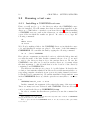
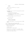
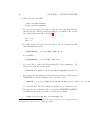
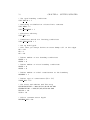
Visualising with Ncview
Ncview is a tool for visualizing netCDF data files. It is very easy to use,
because of its graphical user interface. However, its possibilities are limited.
In order to start this program for a certain data file, type the following
command
ncview riverA_1.tsout2N
When using NcView, you always must give the filename of the data that is
plotted in the command to start the graphical user interface. An example of
the user interface in NcView is given in Figure 2.1. The first thing to do when
working with NcView is selecting the variable to plot. This can be done by
clicking on the name of the variable you want to select. We start by plotting
the sea surface elevation. In order to do so, click on the button with zeta,
which is the name used on COHERENS for the sea surface elevation. In order
to get more information on a variable, click on the button with the question
mark ?.
You should now see a plot of the sea surface elevation, as function of the
x location (on the x-axis) and time (on the y-axis). We can change this by
clicking on the Axes button. If you do so, a dialog box will appear that lets
you select the axes to plot. In this case, there are only two possible options,
the time and the x-dimension. Hence, it is not necessary to change the axes.
Close the dialog box by clicking on cancel. To make the plot larger, click on
the button that says M xn where n is the magnification scale. As you can
see, the image is magnified, and the name of this button is changed to the
new magnification. Press this button again to make the plot even larger.
When can change the colors in the graph by clicking the leftmost button
(its name is one of the color maps, probably 3gauss). Click this button and
see how the colors change. Try out the different colormaps, and select one
you find useful to work with. A useful selection may be ssec. The ranges of
the colorbar are set by the button with Range. Click on it in order to get
a dialog box, in which you can set the limits of the colorbar. You can also
choose to highlight some special ranges by clicking on the button linear. The
name of the button will change in low and the resolution in the color bar
will increase for low values of the water level. By clicking it again, it will say
Hi and have more resolution for high values of the water level. The button
which says Bi-lin will influence the way in which the colors are interpolated
(default is bi-linear interpolation). By clicking it, it will say Repl, which gives
nearest neighbor interpolation. The latter is less visually appealing, but is
28
CHAPTER 2. GETTING STARTED
Figure 2.1: Screenshot of using NcView
is sometimes useful near the edges. Finally, we are going to make some files
of the data. This can be done by clinking on the button Print. A dialog box
will appear. Click on the button File in order to make a file with the data
and click on OK. Use nautilus or konqueror (the Linux programs that do the
same as windows explorer) to look up the file. Click on it to see it. Now click
on umvel to visualize the depth averaged velocities (in the x-direction) and
also make an output file with these data. Finally, close NcView by clicking
on Quit.
We continue by visualizing the 3-D data. In order to open the 3-D file,
type
ncview riverA_1.tsout3N
In this file, three-dimensional data are stored. In fact, because the river test
case is two-dimensional (there is no information in the y-direction), only the
data in the x-z direction can be displayed. We will start by visualizing the
salinity. Click on sal to visualize the salinity. Now, you will see the initial
2.3. POST-PROCESSING THE RESULTS
29
salinity profile in the x-z plane. We can go to a different moment in time by
clicking the arrow to the right. By clicking the two arrows to the right, an
animation is shown. You can change the speed of the animation by sliding
the slider to the right of the text delay. Watch the animation and observe
how the salinity intrusion develops.
Close NcView. We will now continue to make visualizations in Ferret.
2.3.2
visualising with Ferret
Ferret is a more advanced tool for displaying graphics, which has much more
possibilities than NcView. However, it is somewhat more difficult to use than
NcView, since options are given through the command line. Nevertheless, no
real program is necessary to view output, which is different from for example
Matlab.
In order to visualize the data, we must first start Ferret by typing
ferret
Now we are inside Ferret. We can see this, because the command prompt
has changed in yes?. The first thing to do is load the data, with the use
command. Type
use riverA_1.tsout2N
This will load the file riverT 1.tsout2N, with the two-dimensional data. Now
we inspect the variables that are in that file, by typing
show data
You should now see a list with the variables that were saved in the file
riverA 1.tsout2N. We can make contour plots of these data (x and time axis)
by typing
contour zeta
contour umvel
We can also make a graph of the velocity at one location or at one moment
in time by typing respectively
plot umvel[x=50]
plot umvel[t=200]
In this command, the part between the square brackets is used to tell Ferret
which data has to be plotted.
It is also possible to plot various of these data together by typing
30
CHAPTER 2. GETTING STARTED
plot umvel[x=50], zeta[x=50]
plot umvel[x=50], umvel[x=100]
Saving files is somewhat cumbersome in Ferret. The first thing you need to
do is tell Ferret to save every graph it makes as a meta file, which is special
a text file containing the data of the plot. You can do this by typing
set mode metafile
Now make the same contour plots as you did before. When you do not
want to plot any more files, you can type
cancel mode metafile
Now close Ferret by typing
exit
The metafiles that are made by Ferret are text files, with the name metafile.plt.∼nr∼,
in which nr is the number of the file. In order to transform them to graphical
files, which you can use in reports, you have to use the command Fprint
Fprint -o outputfile00.ps -p portrait metafile*.plt
Fprint -o outputfile01.ps -p portrait metafile*.plt.~01~
Note that we used an asterisk (*) in this command, because Fprint changes
the filename every time it is invoked. Note that Fprint prints to a file, so in
order to use it, a default printer must be selected.
Open Ferret again to visualize the three dimensional data
ferret
We first load the three dimensional datafile and see which data it contains
use riverA_1.tsout3N
show data
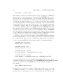
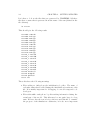
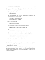
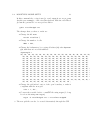
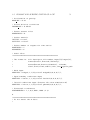
In this file, we can make a vector plot of the velocity field at time step 20
using (an example is given in Figure 2.2)
vector uvel[t=20],wphys[t=20]
We can also make a contour plot of the salinity at this moment in time
contour sal[t=20]
2.3. POST-PROCESSING THE RESULTS
31
Figure 2.2: Screenshot of using Ferret
If we want to plot the vectors and contours together, we must add the overlay
option
vector/overlay uvel[t=20],wphys[t=20]
Once again, we can plot time series or profiles, but now we need to provide
two axis locations between brackets
plot sal[z=1,t=20]
Finally, we make an animation using the repeat statement of the first 50 time
steps. For the animation of the salinity contours, type
repeat/t=1:50/animate/loop=1 (contour sal)
For the animation of the flow vectors, type
repeat/t=1:50/animate/loop=1 (vector uvel,wphys)
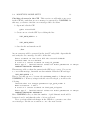
2.3.3
visualising with Octave and Matlab
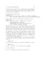
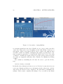
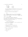
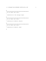
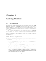
Now we are going to run a second test case, which is called bohai. This test
case is a simulation of the tides in the Bohai Sea (northern part of the Yellow
Sea, see Figure 2.3). The commands are the same as for the previous river
test. Take care of the following
32
CHAPTER 2. GETTING STARTED
Figure 2.3: Map of the Bohai sea
• Edit the defruns file by commenting all lines (i.e. inserting a ’ !’ in the
first column) except the first one such that only the first run is made.
The name of this run is bohaiA. Note that, contrary to the river there
is no spin up run.
• The date of the simulation, which you need to check the advance
of the calculations is in the year 1999 (look this up in the file Usrdef Model.f90). Note that running this test takes about 10–15 minutes
depending on the capacity of your machine.
• When visualizing the data with Ferret, you must define the x and y
data to make time series. Because this case is two-dimensional, there
is only a tsout2N file.
We are using the file bohai 1.1amplt2N with the harmonically analysed
surface M2 -amplitudes as example for making visualisation with Octave or
Matlab.
1. Download the octcdf package, for Ubuntu this is rather straightforward
using
sudo apt-get install octave-octcdf
For other platforms such as Windows a useful wiki might be: http://
modb.oce.ulg.ac.be/mediawiki/index.php/NetCDF_toolbox_for_Octave
2. In this package the ncdump function is included, which provides information about all the contents of the netCDF file. In our example file
2.3. POST-PROCESSING THE RESULTS
33
we see that there are 3 dimensions and 7 variables. The variable we
are interested in is zeta, we are also interested in the dimensions xdim
(longitude), ydim (latitude) and time (depth is constant in this example
so we disregard it).
3. To load a variable to the Octave environment, firstly check whether the
file ncparsen.m has been copied from the scr to your working directory
and type in the qtOctave terminal
[locallat] = ncparsen(’bohaiA_1.1amplt2N’,’xout’)
[locallon] = ncparsen(’bohaiA_1.1amplt2N’,’yout’)
[localzeta] = ncparsen(’bohaiA_1.1amplt2N’,’zeta’)
to load the spatial coordinate arrays xout, yout and the elevation data
zeta.
4. In Matlab (R2008a and higher), you can load variables from the netCDF
file using the ncread function
[locallat] = ncread(’bohaiA_1.1amplt2N’,’xout’)
[locallon] = ncread(’bohaiA_1.1amplt2N’,’yout’)
[localzeta] = ncread(’bohaiA_1.1amplt2N’,’zeta’)
5. To let your graphs appear in a workable screen format, set the display
to the correct environment (only for Octave)
setenv("GNUTERM","wxt")
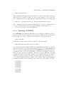
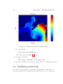
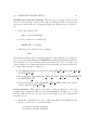
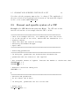
6. Now you can make your first graph
zetafig = localzeta(1,:,:)
contourf(localxout,localyout,zetafig)
7. Add a colorbar by typing
colorbar
8. Put a title and axis legends
title("M2-amplitude","fontsize",20,"fontname","Arial_black")
xlabel("longitude","fontsize",12,"fontname","Arial")
ylabel("latitude","fontsize",12,"fontname","Arial")
34
CHAPTER 2. GETTING STARTED
Figure 2.4: Example figure generated with Octave
9. To export the file
print -dpng bohai_M2amp.png
The result is shown in Figure 2.4.
10. To improve pixel size
print -dpng "-S800,800" "bohai_M2amp.png"
11. For more information on a topic type help topic, for example help print.
2.4
Modifying model setup
Two methods are available to adapt the model settings. In the first one
the model parameters are changed in the CIF. The second one consists in
2.4. MODIFYING MODEL SETUP
35
editing the Usrdef FORTRAN files. The two methods are described in the
subsections below.
2.4.1
Modifying model setup via CIF
2.4.1.1
short CIF introduction
The central input file (CIF) is a functionality introduced in COHERENS V2.1
aimed to define or re-define parameters for model setup without having to
do a recompilation. More information on the format of the CIF file can
be found in the User Documentation. In addition, all forcing data can be
provided in a standard COHERENS format. These formats can be read by
the program without the need to change the model setup code (and recompile
the program) in the Usrdef files.
2.4.1.2
tutorial river test case
The following procedure needs to be used to install the tutorial version of
the river test case
1. Select a working directory, e.g.
cd /home/coherens/riverCIF
2. Create a link with the COHERENS root directory (a path name can be
defined instead of ∼/V2.5), e.g.
ln -s ../V2.5 COHERENS
3. Install the tutorial version of the river test case
COHERENS/install_test -t tutorial/river
4. Adapt your settings by changing coherensflags.cmp.
5. Compile (e.g for Intel Fortran)
make linux-iforts
The following procedure is recommended to run the river test case with the
CIF functionality
1. Open the file defruns
36
CHAPTER 2. GETTING STARTED
river0T,,
river1T,,
which shows that no CIF will be read or produced.
2. Run the test case
./Run
3. The simulation has now created the following input files in standard
COHERENS format:
• riverT.modgrdN: model grid arrays
• riverT.2uvobc1A: open boundary conditions
• riverT.phsfinN: initial conditions produced by the initialisation
run for the final one
4. Run the test case again now using the CIF functionality
cp cifruns defruns
Open the file defruns
river0T,R,river0T.CifModA
river1T,R,river1T.CifModA
5. You may open the CIF files to see how information is passed to COHERENS.
2.4.1.3
changing model setup through the CIF
Now, we are going to change the model by adapting the CIF file and the
forcing files. We will do the following
1. Change the simulation time.
2. Adjust the time step.
3. Modify settings (e.g. roughness length).
4. Change the form of the output file (e.g. from netCDF to ASCII).
5. Modify the grid resolution (number of rows and columns, grid size).
6. Modify the open boundary conditions.
2.4. MODIFYING MODEL SETUP
37
Changing simulation time The first modification is the modification of
the simulation time by editing the CIF file
1. Change the defruns file.
gedit defruns
We will switch off the first of the two simulations for the moment, and
only do changes in the second file
!river0T,R,river0T.CifModA
river1T,R,river1T.CifModA
2. Open and edit the CIF.
gedit river1T.CifModA
Set the simulation time to 1 day by changing the line
CENDDATETIME = 2003/01/06;00:00:00:000
into
CENDDATETIME = 2003/01/04;00:00:00:000
The previous re-setting can also be made by inserting the comment
character ! in the first column of the line with the old definition
!CENDDATETIME = 2003/01/06;00:00:00:000
CENDDATETIME = 2003/01/04;00:00:00:000
3. Run the model with the new simulation time.
./Run
Note that the time steps for the output data are adapted automatically. This
is seen by opening the warlog file
gedit river1T.warlogA
This will show a warning, that the last time step for output is equal to
the last time step in the model. However, if you would have increased the
calculation time, you would have had to adapt the number of time steps that
is outputted manually
38
CHAPTER 2. GETTING STARTED
WARNING: value of integer component %tlims(2) and element 1
of array tsrgpars is set from 8640 to 2880
Check in the output data, that you now have indeed only one day of output
data. You can do this easily using ncdump by typing (use man ncdump to
look up what -v means)
ncdump -v time riverT_1.tsout2N | less
Modification of the time step This exercise is focused on the modification of the time step by editing the CIF file, the instructions are given
below
1. Open and edit the CIF.
gedit river1T.CifModA
2. Set the 2-D time step to 15 seconds. COHERENS also has a 3-D time
step for barotropic calculations, which is given as the number of 2-D
time steps that pass before a 3-D step is done. This is given by the
variable IC3D. In order to leave the 3-D time step unchanged, we modify
this value as well by changing
DELT2D = 30.
IC3D = 10
into
DELT2D = 15.
IC3D = 20
3. Run the model with the new time step.
./Run
Visualize the results.
2.4. MODIFYING MODEL SETUP
39
Checking of errors in the CIF This exercise we will make some errors
in the CIF file, such that an error message is generated by COHERENS. In
this way, you learn to find the error messages and solve them
1. Open and edit the CIF.
gedit river1T.CIF
2. Create an error in the CIF by re-editing the line
IOPT_GRID_NODIM = 3
to
IOPT_GRID_NODIM
3. Save the file and run the model
./Run
An error message will be generated in the river1T.errlogA file. Open this file
and verify the error message. It will look like this
Error occurred on line 29 of CIF file river1T.CifModA
Variable name is not defined
A total of 1 errors occurred in read_cif_params
Error type 7 : Invalid initial values for model parameters or arrays
PROGRAM TERMINATED ABNORMALLY
This message tells you that the syntax in the CIF is not correct. Now we try
to correct this message, but make another mistake. Edit the CIF and type:
IOPT_GRID_NODIM = 4
This is obviously an error, because the maximum number of dimensions in
COHERENS is 3. When you inspect the file river1T.errlogA, you will see the
following
Invalid value for integer parameter iopt_grid_nodim: 4
Must be between: 1 and 3
A total of 1 errors occurred in check_mod_filepars
Error type 7 : Invalid initial values for model parameters or arrays
PROGRAM TERMINATED ABNORMALLY
Here COHERENS tells you that the number of grid dimensions should be
between 1 and 3, and thus the value of 4 is not allowed.
Try to perform additional changes in the CIF file to generate some other
error messages. Fix the errors and move on to the next exercise.
40
CHAPTER 2. GETTING STARTED
Form of the output file In this exercise, we modify the format of the
output file by editing the CIF. The instructions are given below
1. Open and edit the CIF.
gedit river1T.CifModA
2. Change the format of the output file from netCDF to ASCII. Change
the third character of the string
TSR2D = 1,T,N,riverT_1.tsout2N,T,,2
from N to A:
TSR2D = 1,T,A,riverT_1.tsout2N,T,,2
3. Run the model with the new output format
./Run
Now you have a new file, called riverT 1.tsout2N, containing ASCII
output data. Open the file in gedit to inspect the data.
4. Change the current default filename for easy management on the same
input line
TSR2D = 1,T,A,riverT.txt,T,,2
5. Run the model with the new output filename.
./Run
We strongly recommend you to use the netCDF format for your output.
Therefore, undo the changes done during this exercise and continue to the
next one.
2.4. MODIFYING MODEL SETUP
41
Modification of model settings This exercise is focused on the modification of some settings of the model setup by editing the CIF, in the present
exercise we will modify the roughness height, the instructions are given below:
1. Open and edit the CIF
gedit river1T.CifModA
2. Set the roughness to 0.3E-02 [m]
ZROUGH_CST = 0.3E-02
3. Run the model with the new roughness
./Run
Visualize the results, and see what the effects is of the changed bed roughness.
You can modify many things in COHERENS, including the numerical scheme,
the turbulence model and many physical parameters. Try to modify some
other settings, by looking them up in the user manual and seeing what they
do. Interesting settings to change are:
• The numerical scheme for advection, using IOPT ADV SCAL, IOPT ADV 2D
and IOPT ADV 3D
• Horizontal viscosities using IOPT HDIV 2D, IOPT HDIV 3D, HDIFMOM CST
and HDIFSCAL CST
• Vertical turbulence model using IOPT VDIF COEF and the various turbulence switches IOPT TURB *.
Grid resolution This exercise is focused on the modification of the grid
resolution by editing the CIF, as well as the input files. In this way, you get
already a first idea how to set up a new model application. The instructions
are given below:
1. Adapt the defruns file in oder to make sure that both simulations are
run (i.e. remove the ! on the first line)
river0T,R,river0T.CifModA
river1T,R,river1T.CifModA
42
CHAPTER 2. GETTING STARTED
2. Open and edit both CIFs
gedit river0T.CifModA
gedit river1T.CifModA
3. We are now resetting the setup so that the test runs with half the
current grid size. Firstly, change the number of columns of the computational grid from nc=141 to nc=2814
NC = 281
NR = 2
4. Secondly, change the grid size from 1000 to 500 m. Change the fifth
and sixth fields in the line
SURFACEGRIDS = 1,1,0,0,1000.,1000.,0.,0.
in both CIFs to
SURFACEGRIDS = 1,1,0,0,500.,500.,0,0
5. Use a new file to called riverTnew.modgrdN for the bathymetry. We
will generate this file in a moment.
MODFILES = modgrd,1,1,N,R,riverTnew.modgrdN,0,0,0,0,F,F,
6. Also change the eleventh field for the time series output grid (parameter
TSRGPARS, in river1T.CifModA only, from 140 to 280
TSRGPARS = 1,T,F,F,T,2003/01/03;00:00:00:000,3,0,0,1,280,1,1,1,1,1,20
Now save the files. We will continue by making a new bathymetry file.
7. Generate the new bathymetry file. Convert the COHERENS netCDFfile
an ASCII text file that can easily be edited, using ncdump
ncdump riverT.modgrdN > riverTmodgrd.txt
4
The actual number of “active” in the X-direction is given by nc-1. Halving the grid
size means then that nc is reset to 2*(nc-1)+1=281.
2.4. MODIFYING MODEL SETUP
43
In this command the > sign is used to send output from one program
(in this case ncdump) to a file riverTmodgrd.txt. Edit the riverTmodgrd.txt file generated for a new grid resolution
gedit riverTmodgrd.txt
The changes that you have to make are
• Change the file name
netcdf riverTnew {
• Change the number of cells
X001 = 280 ;
• Change the bathymetry, by copying all values (20) after depmeanglb, such that are now 280 numbers
depmeanglb =
20, 20, 20, 20, 20, 20, 20, 20, 20, 20, 20, 20, 20, 20, 20, 20, 20, 20, 20,
20, 20, 20, 20, 20, 20, 20, 20, 20, 20, 20, 20, 20, 20, 20, 20, 20, 20,
20, 20, 20, 20, 20, 20, 20, 20, 20, 20, 20, 20, 20, 20, 20, 20, 20, 20,
20, 20, 20, 20, 20, 20, 20, 20, 20, 20, 20, 20, 20, 20, 20, 20, 20, 20,
20, 20, 20, 20, 20, 20, 20, 20, 20, 20, 20, 20, 20, 20, 20, 20, 20, 20,
20, 20, 20, 20, 20, 20, 20, 20, 20, 20, 20, 20, 20, 20, 20, 20, 20, 20,
20, 20, 20, 20, 20, 20, 20, 20, 20, 20, 20, 20, 20, 20, 20, 20, 20, 20,
20, 20, 20, 20, 20, 20, 20, 20, 20, 20, 20, 20, 20, 20, 20, 20, 20, 20, 2
20, 20, 20, 20, 20, 20, 20, 20, 20, 20, 20, 20, 20, 20, 20, 20, 20, 20, 2
20, 20, 20, 20, 20, 20, 20, 20, 20, 20, 20, 20, 20, 20, 20, 20, 20, 20, 2
20, 20, 20, 20, 20, 20, 20, 20, 20, 20, 20, 20, 20, 20, 20, 20, 20, 20, 2
20, 20, 20, 20, 20, 20, 20, 20, 20, 20, 20, 20, 20, 20, 20, 20, 20, 20, 2
20, 20, 20, 20, 20, 20, 20, 20, 20, 20, 20, 20, 20, 20, 20, 20, 20, 20, 2
20, 20, 20, 20, 20, 20, 20, 20, 20, 20, 20, 20, 20 ;
• Change the grid index location of the open boundary, to make it
compliant with the new grid
iobu = 1, 281 ;
• Convert the text file back to a netCDF file using ncgen (look up
how it works using man ncgen)
ncgen -b riverTmodgrd.txt -o riverTnew.modgrdN
8. The new grid file can also be created alternatively through the CIF
44
CHAPTER 2. GETTING STARTED
• Edit the defruns file and disable the second run
river0T,R,river0T.CifModA
!river1T,R,river1T.CifModA
• In river0T.CifModA change the line
MODFILES = modgrd,1,1,N,R,riverT.modgrdN,0,0,0,0,F,F,
into
MODFILES = modgrd,1,1,N,W,riverTnew.modgrdN,0,0,0,0,F,F,
• Run the test case and replace the ‘W’ again to ‘R’ on the same line
in the river0T.CifModA. The new grid file has now been generated
automatically.
9. Run the model now with the new grid resolution.
./Run
Note that for this exercise, it is necessary to run both simulations (river0T
and river1T), because the initial conditions that are generated in run river0T
are changed with the new grid resolution and need to be provided for river1T.
Modification of open boundaries This exercise is focused on the modification of the definitions of the open boundaries by editing the open boundary
file. The instructions are given below
1. Edit both CIFs files, in order to use a new file with boundary conditions:
MODFILES = 2uvobc,1,1,A,R,riverTnew.2uvobc1A,0,0,0,0,F,F,
2. Open and edit the riverT.2uvobc1A file generated previously, which
contains the open boundaries in COHERENS ASCII format
gedit riverT.2uvobc1A
3. Modify the type of the upstream open boundary condition from the
characteristic method (11) to the method of Flather (8)
ityp2dobu
8
13
4. Modify the the water level amplitude from 0.8 to 1.0 m
2.4. MODIFYING MODEL SETUP
ud2obu_amp
14.00714
zetobu_amp
1.000000
45
0.000000
0.000000
Note that the amplitude of the depth-integrated velocity is proportional
to the water level amplitude in the river test case and needs therefore
be divided by 0.8.
5. Save the file under the new name riverTnew.2uvobc1A
6. Run the model with the new boundary definitions
./Run
2.4.2
Adapting model set up via the Usrdef files
We are now going to repeate the model setup changes by adapting the FORTRAN code in the Usrdef files.
2.4.2.1
installing and running the example test
We re-install, compile and run the tutorial version of river test again, now
without making use of the CIF. The steps are similar to ones shown in the
previous section, but repeated here for clarity
1. Select a working directory, e.g.
cd /home/coherens/rivertest
2. Create a link with the COHERENS root directory (a path name can be
defined instead of ∼/V2.5), e.g.
ln -s ../V2.5 COHERENS
3. Install the tutorial version of the river test case
COHERENS/install_test -t tutorial/river
4. Adapt your settings by changing coherensflags.cmp.
5. Compile (e.g for Intel Fortran)
make linux-iforts
6. Run the test case
./Run
46
CHAPTER 2. GETTING STARTED
2.4.2.2
changing model setup through the Usrdef files
The modifications in the model setup, discussed with the CIF method in
the previous section, can equally well be performed, by modifying the setups
defined in the Usrdef files. Main difference is that you need to recompile
the code each time a Usrdef file has been changed. This recompilation only
takes a few seconds of time.
Changing model setup parameters As before, switch off the first of the
two simulations in defruns
!river0T,,
river1T,,
1. Edit the file Usrdef Model.f90
gedit Usrdef_Model.f90
2. To change the simulation time, modify the following line in routine
usrdef mode params from
CendDateTime = 2003/01/06;00:00:00:000
into
CEndDateTime = 2003/01/04;00:00:00:000
3. Note that, lower case characters are used preferentially for variable
names contrary to the CIF where all parameter names are given in
upper case.
4. Since the comment character ‘!’ has the same meaning in FORTRAN
as for the CIF, you may also comment the old definition
!CEndDateTime = 2003/01/06;00:00:00:000
CEndDateTime = 2003/01/04;00:00:00:000
5. Recompile and run the modified test
make linux-iforts
./Run
2.4. MODIFYING MODEL SETUP
47
6. A new time step is taken by changing the following lines in Usrdef Model.f90
(routine usrdef mod params) from
delt2d = 30.0
...
ic3d = 10
to
delt2d = 15.0
...
ic3d = 20
7. The roughness length parameter zrough cst can be changed in the same
routine.
8. The switch iopt grid nodim is not defined in Usrdef Model.f90. COHERENS will therefore take the default value which is 3. You can reset
this value to the erroneous value of 4 in routine usrdef mod params
(preferentially in section “Switches”) within the file Usrdef Model.f90
...
SUBROUTINE usrdef_mod_params
...
iopt_grid_nodim = 4
...
END SUBROUTINE usrdef_mod_params
9. Compile and run. The same error message as in the CIF example is
issued.
Form of the output file The instructions for modifying the format of an
output file are as follows
1. Edit the file Usrdef Time Series.f90
gedit Usrdef_Time_Series.f90
2. Change the output format by adding the two lines
48
CHAPTER 2. GETTING STARTED
...
SUBROUTINE usrdef_tsr_params
...
tsr2d(1)%form = ’A’
tsr2d(2)%filename = ’riverT.txt’
...
END SUBROUTINE usrdef_tsr_params
in routine usrdef tsr params. The second line changes the name of the
output file as well.
3. Compile and run.
Grid resolution Halving the grid size (in the X-direction) is easily performed by modifying the following lines in Usrdef Model.f90
...
SUBROUTINE usrdef_mod_params
...
nc = 281; nr = 2; nz = 20
...
surfacegrids(igrd_model,1)%delxdat = 500.0
surfacegrids(igrd_model,1)%delydat = 500.0
...
END SUBROUTINE usrdef_mod_params
Contrary to the CIF case, the output grid, the grid index of the open boundary locations and the bathymetry are automatically adapted by the code to
the new grid.
Modification of open boundaries The upstream open boundary condition is reset from the characteristic (11) to the Flather (8) method and
the tidal amplitude of the water level is reset from 0.8 to 1.0 m in Usrdef Model.f90
...
SUBROUTINE usrdef_2dobc_spec
...
ityp2dobu(1) = 8; ityp2dobu(2) = 13
...
amp = 1.0; phase = -halfpi
...
END SUBROUTINE usrdef_2dobc_spec
2.5. FORMAT AND SPECIFIC SYNTAX OF A CIF
49
Note that only the parameter amp needs to be changed. The amplitudes of
the water elevation and depth-integrated current are automatically adapted
by the code in routine usrdef 2dobc spec.
2.5
Format and specific syntax of a CIF
Example of a CIF file for the test case River The CIF used in this
tutorial is shown here as an example what the CIF looks like
!************************************************************
! This is an example CIF file, for running the test case river
! It is the second of two files, which runs the simulation of a
! density current.
! This file uses the tutorial settings
! Written by Alexander Breugem
! April 2012
!************************************************************
! Monitoring parameters
!************************************************************
! In this part, parameters are defined that determine the
! parameters tha are written to the logfiles
!
! Get resonable amount of logdata. Increase the number to obtain more data
LEVPROCS INI = 7
LEVPROCS RUN = 3
! Generate a detailed timing file
LEVTIMER = 3
#
!*************************************************************
! Switches and parameters.
! Do not remove the # above
!
! In this part, parameters are set for the run
! Define grid
IOPT GRID NODIM = 3
50
CHAPTER 2. GETTING STARTED
! Use open boundary conditions
IOPT OBC 2D = 1
! Switching on simulation of baroclinic currents
IOPT DENS = 1
IOPT DENS GRAD = 1
! Calculate salinity
IOPT SAL = 2
! Turbulence switch for limiting conditions
IOPT TURB IWLIM = 1
! Set up model grid
! Note that you always define an extra dummy cell on the edges
NC = 141
NR = 2
NZ = 20
! Define number of sea boundary conditions
NOSBU = 2
NOSBV = 0
! Define number of river boundary conditions
NRVBU = 0
NRVBV = 0
! Define number of tidal constituents at the boundary
NCONOBC = 1
! Define type of constituent (S2 = 51)
INDEX OBC = 51
! Set start and endtime amd Time step
CSTARTDATETIME = 2003/01/03;00:00:00:000
CENDDATETIME = 2003/01/06;00:00:00:000
DELT2D = 30.
IC3D = 10
! Select constant water depth
DEPMEAN CST = 20.
2.5. FORMAT AND SPECIFIC SYNTAX OF A CIF
51
! Accelaration of gravity
GACC REF = 9.81
! Bottom friction coefficient
ZROUGH CST = 0.6E-02
! Define restart files
NORESTARTS = 0
! define runtitle
INTITLE = riverT
OUTTITLE = riverT
! Define number of outputs for time series
NOSETSTSR = 1
NOVARSTSR = 6
! Model files
!************************************************
! The format is: file descriptor,file number,input(1)/output(2),
!
format(A=ascii,N=netcdf,U=binary),
!
status(R=read,W=write,N=usrdef), filename,
!
tlim1,tlim2,tlim3,endfile,info,time regular,path
! Grid input
MODFILES = modgrd,1,1,N,R,riverT.modgrdN,0,0,0,0,F,F,
! Open boundary conditions input
MODFILES = 2uvobc,1,1,A,R,riverT.2uvobc1A,0,0,0,0,F,F,
! Initial conditions input (restart file from simulation 0)
MODFILES = inicon,1,1,N,N,riverT.phsfinN,0,0,0,0,F,F,
! Horizontal coordinates
SURFACEGRIDS = 1,1,0,0,1000.,1000.,0.,0.
#
!**********************************************
! Do not remove the # above
!
52
CHAPTER 2. GETTING STARTED
! Parameters for time series output
!
! Definition of the output variables
! The format is: number (output), key id, dimension (0/2/3),
!
oopt,klev,dep, node,fortran name, long name, unit
! Only the first 3 are required
! Surface elevation (92)
TSRVARS = 1,92,2,,,,,,,,,
! Depth avg U velocity (104)
TSRVARS = 2,107,2,,,,,,,,,
! U velocity
TSRVARS = 3,109,3,,,,,,,,,,
! V velocity
TSRVARS = 4,121,3,,,,,,,,,,
! Vertical velocity
TSRVARS = 5,123,3,,,,,,,,,,
! Salinity
TSRVARS = 6,128,3,,,,,,,,,,
! Matching the variables to sets
! Format: iset, ivar1, ivar2,etc.
IVARSTSR = 1,2,3,4,5,6
! Definition of the output files
! Format: set number, defined (T/F), format (A=ascii,N=netCDF, U=binary),
!
filename, info (T/F), path, header_type
TSR2D = 1,T,N,riverT 1.tsout2N,T,,2
TSR3D = 1,T,N,riverT 1.tsout3N,T,,2
! Definition of output grid
! Format: set number,gridded (T/F),gridfile (T/F),land mask (T/F),
!
timegrid (T/F),ref date,number dimensions,number stations,
!
start x,end x,stepx,start y,end y,step y, ,start z,end z,
!
step z,start time,end time,timestep
! note that the end time may have to change if you change the time step or
! time interval of the simulation
TSRGPARS = 1,T,F,F,T,2003/01/03;00:00:00:000,3,0,0,1,140,1,1,1,1,1,20,1,0,
8640,180
2.5. FORMAT AND SPECIFIC SYNTAX OF A CIF
#
!**********************************************
! Do not remove the # above
!
! Parameters for time averaged output
#
!**********************************************
! Do not remove the # above
!
! Parameters for harmonic analysis
#
!**********************************************
! Do not remove the # above
!
! Parameters for harmonic output
#
53
54
CHAPTER 2. GETTING STARTED