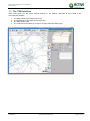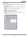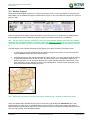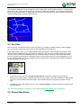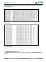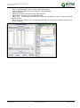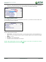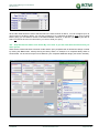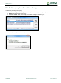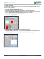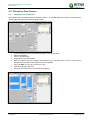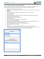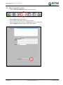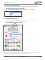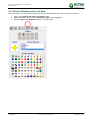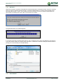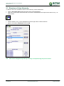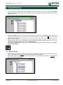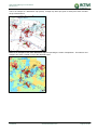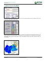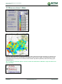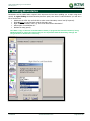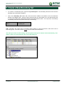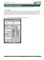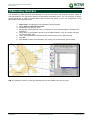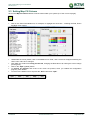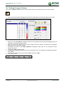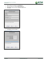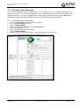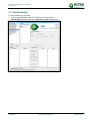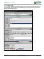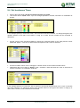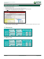
1
Total Solution Mapping User Manual 29/04/2013 Version 2.0 Total Solution Mapping User Manual TSM Version 9.3 February 2015 Total Solution Mapping v9.3 User Manual February 2015 Document Control Confidentiality Statement This document contains information confidential and proprietary to Active Informatics Limited. It shall not be disclosed in whole or part by the recipient to any third party or to any employees other than those who have a need to know such information. The document shall not be duplicated (in part or in whole) or used by the recipient for any purpose other than to evaluate Active Informatics Limited’s products and services. Copyright Notice Copyright © 2015 Active Informatics Ltd. All rights reserved. Registered Address: Network House, Basing View, Basingstoke RG21 4HG. Registered in England No. 6720040. Revision History Version Date Author Change Summary Draft 1a 01/04/2013 Ed Rackstraw Initial drafting Draft 1b 29/04/2013 Ed Rackstraw Updates following review Issue 1 06/06/2013 Marie Mapstone Inclusion of TTB manual Issue 2 01/02/20145 Marie Mapstone Update version number The versions numbered “1a, 1b”, are draft status and therefore can be changed without formal change control. Once a document has been formally approved and issued it is version numbered “Issue 1” and subsequent releases will be consecutively numbered, following formal change control. The version number appears in the header of every page. Confidential www.activeinformatics.com Page 2 of 389 Total Solution Mapping v9.3 User Manual February 2015 TSM User Guide Part 1: Map Functions TSM USER GUIDE PART 1: MAP FUNCTIONS 1 GETTING STARTED 3 20 1.1 Starting TSM 20 1.2 Screen Resolution 20 1.3 The TSM Interface 21 1.4 Toolbox Tabs 22 2 MAP DISPLAY 23 2.1 Map Toolbar 23 2.2 Vector Layers 24 2.3 Key Sites 25 2.4 Refresh Map Button 25 2.5 Motorway Junctions and Railway Stations 26 2.6 Zoom & Pan 27 2.7 Labels 29 2.8 Refresh Map 34 2.9 Copy 34 2.10 Sessions 34 2.11 Tools Launch Button 36 2.12 National Grid Layer 36 2.13 Raster Mapping 37 MAP TOOLBOX 38 3 3.1 Measurement Tools 38 3.2 Concentric Circles 38 3.3 Scale 40 3.4 North Point 41 Confidential www.activeinformatics.com Page 3 of 389 Total Solution Mapping v9.3 User Manual February 2015 3.5 Advanced search (find): 41 3.6 Datum Position 42 3.7 Distance (Between 2 Points) 43 3.8 Grid Reference - Easting/Northing 43 3.9 Longitude/Latitude 44 3.10 Key Site Database Display 44 4 STEP BY STEP (FREQUENTLY USED FUNCTIONS) 46 4.1 Zoom 46 4.2 Pan 46 4.3 Label Street 46 4.4 Vector Layers 46 4.5 Raster Maps 46 4.6 Search Facility (FIND) 47 TSM USER GUIDE PART 2: ONLINE HELP 48 1 49 HELP MENU 1.1 Help Contents 49 1.2 Search for Help on 50 1.3 Context Help 50 1.4 About 51 2 CONTEXT SENSITIVE HELP 52 3 QUICK HELP AND STATUS DISPLAY 53 TSM USER GUIDE PART 3: DB DESIGN 55 1 57 DB DESIGN TOOLBOX 1.1 Designing Databases 57 1.2 How should the data be formatted? 57 1.3 Data Cleansing 59 Confidential www.activeinformatics.com Page 4 of 389 Total Solution Mapping v9.3 User Manual February 2015 2 DATABASE DESIGN WIZARD 60 2.1 Stage 1: Selecting files 60 2.2 Stage 2: Naming the database 61 2.3 Stage 3: Field Definition 62 2.4 Stage 4: Selecting Search Fields 63 2.5 Previewing the Data 64 2.6 Too many unique values warning message 65 2.7 Importing Education Learner Data Example 66 2.8 Importing Ambulance Mobilisation Data Example 68 3 DATABASE IMPORT 70 3.1 Importing Data after Using the Wizard 70 3.2 Reject File 72 3.3 Database List 72 3.4 Overwriting Existing Files 73 3.5 Appending Data 73 3.6 Deleting Database Types and Files 74 4 EDITING & CREATING DATABASE DESIGNS 75 4.1 Manual Database Designs 75 4.2 Copy a Database Type 76 4.3 Field Definition 76 4.4 Whole number fields 77 4.5 Text Fields 78 4.6 Easting and Northing Locators 78 4.7 Date Fields 79 4.8 Time fields 79 4.9 On or After Function 80 4.10 Postcode (Locator) 80 Confidential www.activeinformatics.com Page 5 of 389 Total Solution Mapping v9.3 User Manual February 2015 5 QUERY SCREEN DESIGN 81 5.1 Range Criteria 81 5.2 Selection Lists 81 5.3 Redesign the Query Writer 83 6 IMPORTING DATA MANUALLY 84 7 STEP BY STEP (FREQUENTLY USED FUNCTIONS) 85 7.1 Standard Data Clean Up Methods (CSV files) 85 7.2 Multiple Locators 85 7.3 Resize And Move Boxes On The Query Writer 85 7.4 Delete Database Files and DB Types 86 TSM USER GUIDE PART 4: GRAPHICAL QUERY WRITER 87 1 ACTIVITY TOOLBOX 89 1.1 Selecting a database 89 1.2 Activity Toolbox Functions 90 1.3 Binoculars Button (map toggle) 90 1.4 Pencil Button (redraw) 90 2 QUERY WRITER 91 2.1 Search Boxes 91 2.2 Selection Lists 92 2.3 Count Box 92 2.4 Select All Button 92 2.5 Clear All Button 93 2.6 Selecting List Entries 93 2.7 More than one field per list box 95 2.8 Range Boxes 95 2.9 Setting Date Ranges 96 Confidential www.activeinformatics.com Page 6 of 389 Total Solution Mapping v9.3 User Manual February 2015 2.10 Setting Time Ranges 96 2.11 Include Blanks 96 2.12 Filtering (Dates and Times) 97 2.13 Clearing a Filter 99 3 COLOUR BY 100 3.1 Applying a Colour Theme 100 3.2 When No Selections are Made 102 3.3 Setting Range Field Bands 102 3.4 Date Bandings 102 3.5 Editing band values 105 3.6 Time bandings 106 3.7 Number bandings 106 3.8 Time of Week Bands 107 4 QUERY RESULT 4.1 Execute Query 108 4.2 Changing the Order of Entries 109 4.3 Keeping Dot Colours Static 110 4.4 New query button 111 5 108 STEP BY STEP (FREQUENTLY USED FUNCTIONS) 112 5.1 Date/time filters 112 5.2 Setting bands 112 5.3 Sorting colour-by query 113 TSM USER GUIDE PART 5: MAP DESIGN 114 1 116 DATA AND DISPLAY ANALYSIS 1.1 Introduction 116 1.2 Select which dots to display 116 Confidential www.activeinformatics.com Page 7 of 389 Total Solution Mapping v9.3 User Manual February 2015 1.3 Remove all dots 117 1.4 Show all dots 117 1.5 Toggle the dot map on or off 117 2 SAVE QUERIES 118 2.1 Edit query card details 118 2.2 Save queries to the card stack 118 2.3 Delete query cards 119 2.4 Save queries to the database library 120 2.5 Retrieve a query from the database library 120 2.6 Delete a query from the database library 121 3 DOT SIZE AND SORTING 3.1 Why change the dot size? 122 3.2 Fixed/Standard Size 122 3.3 Size by Geo-group 123 3.4 Label record counts 124 3.5 Size by value 125 4 122 DATA QUERY TIPS 126 4.1 Fire Data Queries 126 4.2 Education Data Queries 130 5 MERGE DOT MAPS 134 5.1 Saving the dot image 134 5.2 Merging the dot image 134 6 SELECTING DATA 6.1 Irregular polygon 137 6.2 Inverting a Polygon 138 6.3 Naming the polygon 138 Confidential 137 www.activeinformatics.com Page 8 of 389 Total Solution Mapping v9.3 User Manual February 2015 6.4 Create a sub-set of the original data. 139 6.5 Removing the polygon from the map 140 6.6 Display a saved polygon 140 6.7 Delete a polygon 140 7 ACTIVITY RECORD LIST 141 7.1 Copy activity record list to clipboard 142 7.2 Print activity records 142 8 STEP BY STEP (FREQUENTLY USED FUNCTIONS) 143 8.1 Re-size dots 143 8.2 Set dot size bands 143 8.3 Draw a polygon to select records 143 8.4 Merging activity (dot) queries 144 TSM USER GUIDE PART 6: KEY SITES 145 1 INTRODUCTION 147 1.1 Key Sites Toolbox 2 KEY SITE IMPORT 2.1 Typical data fields 149 2.2 Key Sites Import Wizard 149 3 147 149 CREATE KEY SITES MANUALLY 152 3.1 Name the database 152 3.2 Add a key site record 153 3.3 Assign a symbol 154 3.4 Display the key site on the map 155 4 EDIT KEY SITE DETAILS 156 4.1 Edit records 156 4.2 Change a Key Site Icon 157 Confidential www.activeinformatics.com Page 9 of 389 Total Solution Mapping v9.3 User Manual February 2015 4.3 Remove a Key Site Button 158 4.4 Export Key Site Data 158 4.5 Refresh Database with new data 159 5 KEY SITE FILTER 162 5.1 Filtering sites on the display 162 5.2 Disable a filter 163 5.3 Clear a filter 163 6 KEY SITE PIE CHARTS 164 6.1 Displaying values as pie charts 164 6.2 Hide pie charts 166 6.3 Remove pie charts 166 7 STEP BY STEP (FREQUENTLY USED FUNCTIONS) 167 7.1 Add a new record 167 7.2 Filtering 167 7.3 Creating pie charts 167 7.4 Import BMP, JPEG or transparent GIF 168 TSM USER GUIDE PART 7: PRINT AND EXPORT 169 1 171 INTRODUCTION 1.1 Print Toolbox 171 1.2 Print Set-Up 171 1.3 Print Content 172 1.4 Print page 173 1.5 MS Word™ Report Writer 174 1.6 MS Excel™ Export 180 1.7 Export to CSV File 183 1.8 Export Eastings & Northings 183 Confidential www.activeinformatics.com Page 10 of 389 Total Solution Mapping v9.3 User Manual February 2015 1.9 2 Printing from other parts of TSM 184 STEP BY STEP – FREQUENTLY USED FUNCTIONS TM 185 2.1 Copy and paste into MS PowerPoint 185 2.2 Create a CSV file and re-import a sub-set of the original data. 185 2.3 Tag data with ref areas/easting and northing 185 TSM USER GUIDE PART 8: AREA GROUPS 186 1 188 1.1 2 INTRODUCTION What are Area Groups? 188 CREATING AREA GROUPS 189 2.1 Select a definition 189 2.2 Area Definition Name 190 2.3 Structure of Area Hierarchy 191 2.4 Area Definitions 192 2.5 Rename Definitions 193 2.6 Define the Area 194 2.7 Alternative Area Selection Methods 195 2.8 Saving Area Definitions 195 2.9 Copy Area Groups 196 2.10 Reset the Map 196 2.11 Area Groups Check Box 197 3 AREA SELECTION TOOLS 198 4 AREA DIRECTORY 199 4.1 Atomic Area 199 4.2 Area Selection List 200 4.3 Switch All On / Off 200 5 DISTRICTS AND WARDS AREA GROUP Confidential www.activeinformatics.com 202 Page 11 of 389 Total Solution Mapping v9.3 User Manual February 2015 6 STEP BY STEP – FREQUENTLY USED FUNCTIONS 203 6.1 How to create an area group 203 6.2 Using Area Groups with Reference 203 6.3 Selected area counts 203 TSM USER GUIDE PART 9: REFERENCE AREAS AND CENSUS DATA 204 7 INTRODUCTION 205 8 CENSUS CATEGORIES 206 8.1 Census Tables 207 8.2 Data Selection 208 8.3 Saving to the Library 212 8.4 Export to Excel 213 9 ANALYSING DEPRIVATION DATA 214 9.1 Creating Deprivation Maps 214 10 STEP BY STEP – FREQUENTLY USED FUNCTIONS 10.1 Run a census query and display it 218 10.2 Select an area 218 10.3 Print/export compare table and key 218 218 TSM USER GUIDE PART 10: COMPARISONS AND STATS 219 11 INTRODUCTION 221 11.1 Show Data card 222 11.2 Show Counts Only Mode 223 12 COMPARISON 12.1 Base Data card 224 12.2 Base Area Setting 224 12.3 Show over base % Mode 225 12.4 Display areas by... 226 Confidential 224 www.activeinformatics.com Page 12 of 389 Total Solution Mapping v9.3 User Manual February 2015 12.5 Summed 228 12.6 Comparing Two Data Sets 229 12.7 Statistical Banding 230 12.8 Turning Bands Off And On 232 12.9 Clear Show and Base Data Cards 232 12.10 Map Colours 232 12.11 Education Mapping 235 12.12 Display Statistics Button 241 12.13 Copy Comparison Figures Table to Clipboard 241 13 AUTO-GRID 242 13.1 Creating a Hotspot Map with Auto-grid 14 CONTINUOUS SURFACE MAPPING 14.1 Creating a Hotspot Map with CSM 244 14.2 How CSM Works 245 15 STEP BY STEP – FREQUENTLY USED FUNCTIONS 15.1 Setting stats band values 248 15.2 Percentage comparisons 248 15.3 Hot-spots (Continuous Surface Mapping) 248 15.4 Working out Population Density 249 242 244 248 TSM USER GUIDE PART 11: BOUNDARIES 250 1 INTRODUCTION 252 2 LOADING BOUNDARIES 253 3 DEFAULT PROPERTIES 254 3.1 Current Boundary Set 254 3.2 Hierarchy and Display Switches (Light Bulbs) 255 3.3 Boundary Structure and Display Switches 256 Confidential www.activeinformatics.com Page 13 of 389 Total Solution Mapping v9.3 User Manual February 2015 3.4 4 Pop-Up Menus 257 INDIVIDUAL PROPERTIES 258 4.1 Property Grid 259 4.2 To change the font: 260 5 CREATE A NEW BOUNDARY SET 261 5.1 Renaming a Boundary Set 262 5.2 Rename Level 262 5.3 Create New Level 262 5.4 Create a Boundary Group 263 5.5 Create a Boundary Beneath the Current Group 263 5.6 The Centroid 264 5.7 Create Boundary Outline (Draw) 264 6 CALCULATION AND THEMATIC 267 6.1 Datasets 267 6.2 Modify by 268 6.3 Result Formula 268 6.4 Calculate 268 6.5 Displaying the Stats on the Map 269 6.6 Band Values 269 6.7 Printing the Calc And Theme Banding Key 270 6.8 Show / Hide Results Sheet 270 6.9 Results Sheet Tools 271 6.10 Clear Dataset Cards 271 7 MAKE USER POLY 272 8 SAVE BOUNDARY SETTINGS 273 9 EXPORTS AND BOUNDARY SETS 274 Confidential www.activeinformatics.com Page 14 of 389 Total Solution Mapping v9.3 User Manual February 2015 9.1 Export Activity Data to a CSV File 274 9.2 Export Boundaries To Mid/Mif Files 274 9.3 Import a Mid/Mif Boundary File 275 10 BOUNDARY GRID SET 276 11 CONVERT BOUNDARIES INTO REFERENCE AREAS 277 12 STEP BY STEP – FREQUENTLY USED FUNCTIONS 278 12.1 Turning boundaries on/off 278 12.2 Export data through boundaries 278 12.3 Calculation and Thematic 278 12.4 Import MID/MIF 279 12.5 Create new boundary 279 12.6 Create new Reference Area from a boundary 279 TSM USER GUIDE PART 12: SITE SYMBOL DESIGN 280 1 INTRODUCTION 281 Guide to the Panels 282 1.1 2 CREATING AND EDITING SYMBOLS 285 2.1 Create a new symbol 285 2.2 Review a Symbol 288 2.3 Re-scale a symbol 288 2.4 Edit a Symbol 289 3 IMPORTING BMP, GIF AND JPEG FILES 293 4 FILE MENU 294 5 HELP MENU 295 TSM USER GUIDE PART 13: ACTIVE CONFIGURATION 296 1 297 INTRODUCTION Confidential www.activeinformatics.com Page 15 of 389 Total Solution Mapping v9.3 User Manual February 2015 2 COLOUR CONFIGURATION 298 2.1 Setting Dot Colours 298 2.2 Setting Map Line Colours 299 2.3 Setting Map Fill Colours 300 2.4 Setting Compare Colours 301 3 PLACENAME CONFIGURATION 302 3.1 Adding Placenames 303 3.2 Deleting Placenames 303 4 4.1 POSTCODE CONFIGURATION 304 Adding Postcodes 304 TSM USER GUIDE PART 14: ACTIVE INDICES 305 1 306 INTRODUCTION 1.1 Import a New File or View Data 306 1.2 View Existing Data Tables 306 1.3 File Format 308 1.4 Data Restrictions 308 1.5 Importing New Data 309 1.6 Deleting Data 314 1.7 Using the Data with TSM 314 TSM USER GUIDE PART 15: ACTIVE ALIAS 315 1 INTRODUCTION 316 2 SETTING UP THE CONVERSION TABLES 317 2.1 Importing Data into Tables 317 2.2 Creating Tables Manually 318 3 3.1 CONVERTING FILES USING THE TABLES File Format Confidential 321 321 www.activeinformatics.com Page 16 of 389 Total Solution Mapping v9.3 User Manual February 2015 3.2 File Selection 322 3.3 Field Selection 323 3.4 Table Selection 324 3.5 Converting a File 325 3.6 Saving the converted file 326 4 HELP AND EXIT 327 4.1 Quick Help & Program Status 327 4.2 Online Help 327 4.3 Exit 327 TSM USER GUIDE PART 16: ACTIVE NLPG 328 1 INTRODUCTION 329 1.1 NLPG Data Format 330 1.2 Settings in the Provider.ini File 330 2 NLPG IMPORT 331 3 USING THE UPRN AS A LOCATOR IN TSM 334 TSM USER GUIDE PART 17: ACTIVE ADDRESS GENERATOR 336 1 INTRODUCTION 337 2 MATCHING DATA WITH STREET ADDRESSES 338 3 SAVING THE FILE 340 TSM USER GUIDE PART 18: ACTIVE LIFESTYLE DATA 341 1 INTRODUCTION 342 2 UPDATING THE LIFESTYLE DATABASE 343 3 TAGGING YOUR OWN DATA 346 3.1 Input File Format Confidential 346 www.activeinformatics.com Page 17 of 389 Total Solution Mapping v9.3 User Manual February 2015 3.2 What Will Be Added? 346 3.3 Starting the Matching Process 347 3.4 Selecting the Input File 348 3.5 Locator Field 349 3.6 Grid Search Tolerance 350 3.7 Lifestyle Data Selection 351 3.8 Processing the Data 352 3.9 Saving the Extract File 353 3.10 Viewing the Reject File 353 TSM USER GUIDE - TRAVEL TIME BOUNDARIES 354 4 INTRODUCTION 356 5 MAP DETAIL PANEL 357 5.1 Features 357 5.2 County and District Borders 357 5.3 Importing Boundaries 358 5.4 Isochrones 359 5.5 Key Sites 359 5.6 Pins 360 5.7 Manipulating the Map 360 5.8 Distances/Points 360 6 MAP FEATURES 6.1 Road Properties 361 6.2 Point Properties 362 6.3 Road Filter 364 6.4 Road Selection 364 7 361 SESSIONS Confidential 365 www.activeinformatics.com Page 18 of 389 Total Solution Mapping v9.3 User Manual February 2015 8 DRIVETIME RULES 8.1 Core road speed files 367 8.2 Variance files 370 8.3 Override rules 373 9 366 DRIVETIME TOOLS 375 9.1 Drivetime Tools Panel 375 9.2 New Isochrone Set Panel (parameters) 376 9.3 Creating Isochrones 377 9.4 Set Isochrones Times 378 9.5 Placing a Pin in the Map 379 9.6 Generating Isochrones Manually 380 9.7 Generating Isochrones Automatically Using Key Sites: 380 10 DRIVETIME/TRACKBACK 10.1 Selected pin 382 10.2 Mouse click 382 11 DISTANCES GENERATOR 383 12 EXPORT TRAVEL TIME BOUNDARIES 385 12.1 Export To A New Boundary Set 386 12.2 Export to An Existing Boundary Set 386 13 ROAD SPEED GUIDE 387 14 STEP BY STEP – FREQUENTLY USED FUNCTIONS 388 14.1 First Set Up a “Closed Road” Rule 388 14.2 Next Set Up the Parameters 388 14.3 Then Build the Isochrones 388 14.4 Finally Export the Travel Time Boundaries Into TSM 388 Confidential 382 www.activeinformatics.com Page 19 of 389 Total Solution Mapping v9.3 User Manual February 2015 1 Getting Started 1.1 Starting TSM To start the program: Double click the Active TSM Desktop icon or double-click on ‘Provider.exe’ in Windows Explorer. Click OK to select the default geography option ‘2001 Census Wards’ Select ‘No’ when prompted to open the default session (see section 2.1 below). Older systems map have “2001 Census OAs” as an alternative, slightly more detailed, geography, so choose this instead. 1.2 Screen Resolution The native resolution for Active is 1280x1024. It is also possible to run TSM at lower resolutions (e.g. 1280x768 on widescreen laptops) or at higher resolutions on large monitors (e.g. 1900 x 1050). Confidential www.activeinformatics.com Page 20 of 389 Total Solution Mapping v9.3 User Manual February 2015 1.3 The TSM Interface When TSM opens you will notice several features on the window, described in more detail in the accompanying chapters: 1. 2. 3. 4. The Map Toolbar (top left above the map). The Card Stack to save data queries (top right). The Map Window (left). The Toolboxes that enable you to import, analyse and export data (right). 1 2 3 4 Confidential www.activeinformatics.com Page 21 of 389 Total Solution Mapping v9.3 User Manual February 2015 1.4 Toolbox Tabs The Toolbox Tabs (such as the Map Tab below) include a variety of functions to enable you to import analyse and export your data. Detailed explanations are available in the following chapters but, for now, there follows a brief description of each one: 1. Map tab – Find places, create circles round key sites, view key site attributes, and add north arrow and scale bar to map. 2. Database tab – Shows all databases loaded in TSM. You MUST select the database before you go to the Activity tab. 3. Activity tab – Query the data from the database you have just selected. 4. Reference tab – Contains the census or index of deprivation data depending on which you load into the system. 5. Compare tab – Produce thematic and hot spot maps. 6. Print tab – Print maps and export data to MS Excel, MS Word. 7. Areas tab – If you want to look at different geographies. 8. Key Sites tab – Load POI data and assign a symbol to plot on the map e.g. your HQ. 9. DB design tab – Load incident, patient, learner, employer data etc in here; change how the data is viewed in the Activity tab. 10. Boundary tab – Load and import boundaries in to the system. 1 2 3 4 5 6 7 8 9 10 Confidential www.activeinformatics.com Page 22 of 389 Total Solution Mapping v9.3 User Manual February 2015 2 Map Display The map display in Total Solution Mapping (TSM) is where census data, user activity data and comparisons of various combinations of these can be displayed against a geographic backdrop. The size/position of the map, the quantity of geographic detail, and the display of the various data elements is controlled mainly from the map toolbar (above the map) and the map toolbox (the first tab to its right). 2.1 Map Toolbar Below is an example of the map toolbar that sits directly above your map. The following sections will describe the different functions in detail. Confidential www.activeinformatics.com Page 23 of 389 Total Solution Mapping v9.3 User Manual February 2015 2.2 Vector Layers Because the default digital mapping is in vector format (points, lines, curves, and shapes or polygons) the Map Display can be divided into layers to enable either a basic or very rich background image on to which to plot your data. Note: An example of the layers can be found above in blue text. The ‘FILL’ check box is a shading facility that only affects the layers: Settlements, Water Features, and Other Features (e.g. woodland). TIP: The more layers that are switched on, the more time the Map Display will need to be redrawn each time the map Refresh button is clicked. Work with minimum layers until you need to add extra detail behind your data to put it in context. Ideally, switch on extra map layers only when you zoom in. The Map display can be further developed by the display of the layer containing secondary routes: 1. To do this lick on the Secondary Routes and Streets check boxes to place an X in them and then click the Refresh button (the yellow pencil above). 2. Individual elements of the road and rail network can be turned on or off by right-clicking the Primary or Secondary Routes layers above the map. The Street layer can be configured to appear at a specific map zoom. To do this simply Right-click the word “Streets” above the map and set a new zoom value (e.g. 10 km). Below is a vector map of Basingstoke, showing streets, with (red) Local Government Ward outlines displayed on top. TIP: Right-click anywhere on the map and select “Refresh map” instead to redraw the image. Large and Small Urban area Fill can be turned on and off by right-clicking the Settlements layer. Also individual types of water body or woodland feature can be turned on or off by right-clicking the Water or Other features layers above the map. Once all the layers have been checked on, the Map Display becomes very rich and colourful, with considerable detail. Confidential www.activeinformatics.com Page 24 of 389 Total Solution Mapping v9.3 User Manual February 2015 The settlement Text layer can be configured to have a white halo around the place names. To do this simply Right-click on the “Text” layer above the map and select “Settlement Text Halo”. The example below shows the place name “Basingstoke” in capitals with a white halo around the letters to make is stand out against the dark blue background of a shaded statistical map. 2.3 Key Sites Key site records, sometimes known as Point of Interest (e.g. colleges, hospitals, stations, public buildings etc.) must include a postcode or grid reference that falls within the full map area. In the "Map Display" panel, you can display up to 10 Key Site buttons, each with different symbols, which represent different databases (Key Site types). A maximum of ten groups of symbols can be shown at any K more databases can be created and stored. These Key Site buttons will display one time; however many e icons on the map, representing the individual locations of the records within the Key Site databases. Five of y have been configured in the example below, meaning that five different databases the ten available buttons can be represented on the map. S i t e b u t t If you click on the oone or more Key Site symbol buttons a selection of different symbols will be n Display. Note that the button stays pressed in and that revealed in the Map Display displayed in the Map are one or more symbols of the same design. Each symbol depicts the geographic position of a Key s Site. To remove the Key Site symbols from the map, click each button in the Key Site Panel so that they are seen to "pop out". TIP: After each Key Site is clicked or off, the Map Display auto-redraws for convenience. 2.4 Refresh Map Button Confidential www.activeinformatics.com Page 25 of 389 Total Solution Mapping v9.3 User Manual February 2015 Click the map Refresh button (yellow pencil above the map) that will, for example, redraw the Map Display without the Key Site symbols being displayed. Alternatively hit the F5 key on your keyboard. 2.5 Motorway Junctions and Railway Stations Motorway Junctions and Railway Stations are normally displayed on the vector maps y default, although you may need to zoom in to see them in detail. For example, a map size of 5km will enable you to see a particular motorway junction number. If you need to turn the nodes off to prevent the map from becoming too cluttered, ensure that the line in c:\program files\active\provider.ini, in the [Settings] section, is set to the option to Display_Nodes=0 (or Display_Nodes=false) making it clearer, for example in a large city where there may be many railway stations, as per the map of London below. To turn the nodes back ON set it option to “Display_Nodes=-1 or Display_Nodes=true”. When you next open Active the node will no longer appear on the map, TIP: Add a line “Display_NodeMultiplier=20” to increase the size of the nodes. You can adjust the value (20) by editing it to a size appropriate to your map. Confidential www.activeinformatics.com Page 26 of 389 Total Solution Mapping v9.3 User Manual February 2015 2.6 Zoom & Pan To focus on a particular part of the map in the Map Display, use the zoom tools, which are grouped together above the map, to the right of the map size indicator (shown below left). 2.6.1 Zoom In To display part of the entire map in the Map Display, in greater detail: 1. If you click on the Zoom-In tool, which will stay pressed in, and return the cursor to the Map Display, the default cursor has changed to a position cursor +. 2. Next place the cross approximately at any corner of the area you wish to select, left-click and hold the mouse button down. Notice that the cursor has changed to the direction cursor indicating that the cursor may now move in any direction. 3. As the cursor is moved in any direction diagonally, a Zoom Box will be displayed over the map (see example below) showing the area that will be included within the new Map Display, and the greatest dimension of the rectangle being displayed in both km (kilometres) and mls (miles) in the Map Size Indicator. 4. When the rectangle or square zoom box has captured the area of interest, release the mouse button and a more detailed map will be shown based on the longest side of the zoom box. You have now zoomed into an area of the entire mapping available. The horizontal and vertical distance across the mapping in the Map Display is now displayed in the Map Size Indicator in both km and mls. Confidential www.activeinformatics.com Page 27 of 389 Total Solution Mapping v9.3 User Manual February 2015 1. Alternatively it is also possible to zoom in and out in by 50 percent (or out by 200 percent) of the current map size, using the scroll bar underneath the set of zoom buttons. TIP: Active will allow you to zoom down to a map size of 500x500 metres. Please Note: The Zoom-In tool and the position cursor remain activated until cancelled (right-click) thereby allowing a repeat of the above operation. If the mapping now displayed is satisfactory, then click the Zoom-In button (or right-click the map) to cancel the instruction and return the cursor to the default cursor. 2.6.2 Previous Zoom To reverse the zooming in process, click the Previous Zoom tool and the mapping in the Map Display will be redrawn as it was before the last zoom. Active will remember the last 20 zooms/pans in the order in which the Map Display is zoomed in and/or panned. By repeatedly clicking the Previous Zoom tool, the Map Display, will return to the entire original mapping. TIP: Please note that the zoom box can be commenced anywhere within the current Map Display. Smaller settlements’ names also appear the closer to the ground you go. Having obtained suitable new mapping in the Map Display, please note the new Map Size Indicator readings above the top left-hand side of the map. 2.6.3 Pan Map Pan Map can only be used when the map display is already zoomed in. 1. To do this, click on the Pan Map tool, which will stay pressed in, and then return the cursor to the Map. The cursor changes to a “hand” symbol. 2. Left-click and hold the mouse button on the point of the map, which is to be moved. . 3. Drag the cursor to the required position. The original you clicked on is moved to this new position. 4. Alternatively, when you hover over the edges or corners of a zoomed-in map, an arrow will appear, allowing you to pan in that direction, by 50% of the current map size. TIP: When you reach the extreme edges of the map, the computer will beep (where a speaker is present on the PC) indicating that the map cannot be panned any further in that direction. Confidential www.activeinformatics.com Page 28 of 389 Total Solution Mapping v9.3 User Manual February 2015 2.6.4 Zoom Cancel Alternatively, from a zoomed-in Map Display, you can return immediately to the full extents of the map, by clicking the Zoom Cancel tool. Please note: This operation will also clear the Zoom-Out memory. 2.7 Labels This facility can insert labels on the map to: Create a label for a Defined Area (e.g. Ward, Output Area etc). Create a label for a Key Site (point of interest). Change the Background Colour and Foreground Colour and Font. Move one of the labels created. Hide one of the labels created. Delete all labels created using “Label List”. These options are available by right clicking anywhere on the map, e.g. to label an area, right click on the map and choose option “Label area...” Please Note: The “Display areas by:” list in the top-right hand corner controls the area group level and therefore also the associated label. I.e. if this is set to “Ward” a ward name will appear. Set “Display areas by:” to Output Areas to label these instead. Confidential www.activeinformatics.com Page 29 of 389 Total Solution Mapping v9.3 User Manual February 2015 2.7.1 Label Area Click the Label Area option and the Name of the Area will automatically be inserted in a label and displayed on the map. At the same time, the ‘Label Properties’ window similar to the one right will be displayed over the “Area List” in the top right of the screen. Click on the OK button to accept the label or the CANCEL button to remove both label and ‘Label Properties’ window. 2.7.2 Label Site To label a “point of interest” right click on the map, near the chosen Key Site symbol and then select the Label Site option. The name of the Key Site will be inserted in a label and displayed on the map with the same ‘Label Properties’ window as above displayed over the “Area List” in the top right of the screen. Click on the OK button to accept the label or the CANCEL button to remove both label and ‘Label Properties’ window. 2.7.3 Label Properties To view the properties of a label click, RIGHT-click on a label, and the following pop-up appears: If you select option “label properties” the following properties can be set: the font, font size, font colour and font style of the label text the background colour of the label (and pin) the pin style to use the label outline can be turned on or off display the label with solid or transparent backgrounds or with a white halo around the text the minimum and maximum zoom values at which the label will appear. Confidential www.activeinformatics.com Page 30 of 389 Total Solution Mapping v9.3 User Manual February 2015 For example, click on the “Background Colour” button and then on the coloured square from the palette that is required e.g. Green (as highlighted below). Click on the OK button and the label will now have a black text on a green background (as below). The ‘Font/Forecolour’ button displays the properties of the text in the labels in a Windows TM style. TIP: The thickness of the label’s pin can be changed by clicking on the pick list beside the “Pin style” text box (shown above). If no pin is selected then the label will be placed, on the centre of the symbol, closest to the cursor when initially clicked on the map. Confidential www.activeinformatics.com Page 31 of 389 Total Solution Mapping v9.3 User Manual February 2015 Click on OK for the changes made to take place take place or CANCEL for the previous settings to be reinstated. 2.7.4 Label Min And Max Zoom Levels By adjusting the zoom levels you can specify at which level of zoom at which you want the label to appear on the map e.g. between zero and 20km. 2.7.5 Move Label If you RIGHT-click on a label as above and select the ‘Move label’ option. Click the label with the left mouse and drag it to the desired position on the map Right-click to refresh the map. PLEASE NOTE: the cursor will not be allowed out of the map area until this last action is carried out. TIP: If the cursor is located at the square indicating the join of the Pin to the Label, the cursor will change to a black cross enabling the point where the pin joins the label to be moved. 2.7.6 Hide Label 2.7.7 If you RIGHT-click on the label containing the Key Site and select the ‘Hide Label’ option the label will automatically be removed from the map but it is still present within the list. Label List To access the full list of labels, RIGHT-click on a label as above and select the ‘Label list’ option. The following panel is displayed at the top right of the screen: Confidential www.activeinformatics.com Page 32 of 389 Total Solution Mapping v9.3 User Manual February 2015 2.7.8 Select Multiple Labels To allow manipulation of several labels at the same time, click on the first one holding down the mouse button and drag down to highlight all labels within the list (or hold down the CTRL key and left-click to select): The buttons at the bottom of the panel will become available. Click on the Delete button and the window (below) will be displayed and clicking OK will refresh the map with the label(s) removed. TIP: The last option in the pop-up panel (label list) will only appear when labels already exist. Labels can also be saved with a session for frequent use. 2.7.9 Label Nearest Postcode When you right-click on the map, the "Label Nearest Postcode" option appears. Upon selecting this option, a disclaimer appears stating that, "This function finds the nearest Postcode Centroid". This is because Active uses Ordnance Survey Codepoint postcode locations that centre postcodes on groups of housing, rather than on specific properties, so labels and postcode-located data may appear relative to the range of properties (e.g. 250 to 279 Abbey Road) for a particular postcode, not a particular street address. If you click "OK", the label is created, with default properties (white background, black text, Arial font, bold, size 8). The label pin joins the map, where the postcode centroid is located. Locating postcodes accurately can assist when plotting Key Sites and Dot data. Confidential www.activeinformatics.com Page 33 of 389 Total Solution Mapping v9.3 User Manual February 2015 2.8 Refresh Map When you right-click any part of the map and select the ‘Refresh Map’ option, this carries out effectively the same procedure as the ‘Refresh Map Button’ (see above). 2.9 Copy When you right-click any part of the map and select the ‘Copy’ option, this places exactly what can be seen TM on the map at that time onto the clipboard ready to be pasted into any other Microsoft package (e.g. Word or PowerPoint). 2.10 Sessions You can change sessions by double-clicking on an existing session name in the list. To create a new session name, double-click the item '<new>' and type in a session name. Then press the ENTER key on the keyboard. An existing session may be deleted by highlighting it and pressing the delete key - you are prompted before the delete is executed. Press ESC or click elsewhere to cancel and/or dismiss the list. Please Note: Changing the current session name does nothing except just that - data is not automatically restored nor saved- you must explicitly use the session restore or session save buttons for anything to happen with the new session. Sessions exist as subdirectories in the file system and as such the names are limited to 150 characters in length. No filename extension or spaces are permitted (use underscores _ instead of spaces). You may not delete a session if it is the currently active one. Neither may you delete the session named 'Default' within the program, because Active expects this session to exist at all times, while the program is running. 2.10.1 Session Save Button Clicking this button saves the current session's working data to the default or named session relating to the Reference Area Set you are using (e.g. Census 2001 OAs). Session variables that are saved: Map settings; includes: zoom history, map layers selected, key site toggle states/filters, picked areas, concentric circles and labels. Area settings; includes: area definition in use, area selections. Compare settings; includes: Show & Base levels, Show & Base cards, statistical bands, shading style & options, graph settings. The entire contents of the card stack. The episode card and all data required to recreate the query that generated the card. Confidential www.activeinformatics.com Page 34 of 389 Total Solution Mapping v9.3 User Manual February 2015 The census card and current census display mode. The Boundaries which are currently set to be displayed. 2.10.2 Session name This box shows the current session name and gives access to the session inventory. When Active is launched the session name is set to 'Default' if chosen, or a temporary session that is date and time stamped. You may choose to save and restore session data to/from different named sessions as described above. Clicking on the session name box will pop up a list or inventory of existing named sessions: 2.10.3 Session restore button Clicking this button restores a previously saved working session. The session data is restored from the default or named session. The current working session data is discarded. Confidential www.activeinformatics.com Page 35 of 389 Total Solution Mapping v9.3 User Manual February 2015 2.11 Tools Launch Button At the top-left of the map display is a button enabling you to launch the Active utility programs (tools) that are provided as part of the software package. N.B. These buttons will only launch the utilities if the relevant utility programs are resident in C:\Program Files\Active folder on your PC. Active Configuration - Change the map colours, place names and postcodes to suit your needs. Active Alias - Convert numerical codes into text descriptions. Active Indices - Generate tables of information for use with census comparison Active Key Sites - Create unique map symbols for use with Key Site databases. Active Data Config – Allows you to prepare a file for input into the system. Active Address Generator – Enables you to create a list of street addresses from postcodes. Active Lifestyle Match – Allows you to match your data with lifestyle characteristics. 2.12 National Grid Layer The National Grid map layer can be displayed as grid lines on the map denoting 100 kilometre grid squares (or 'tiles'). Click on the National Grid layer (above the map under Activity and Statistics). Redraw the map (the pencil button). The National Grid lines are now displayed on the map. Confidential www.activeinformatics.com Page 36 of 389 Total Solution Mapping v9.3 User Manual February 2015 2.13 Raster Mapping Ordnance Survey (OS) Raster files make the maps more detailed and can be displayed, in colour or greyscale, on their own or in combination with the traditional Vector mapping (see above). Click the “Raster” radio button to display the raster map (see examples below). Zoom in closer to see more detail. Switch on activity dots, key sites or hotspot maps and redraw to overlay these on top of the raster image. The opacity of dots can be altered, using the slider, from 0% (solid) to 100% (transparent) overlaid on top of the map (below middle). Click the “Raster & Vector” radio button, switch on boundaries and redraw to overlay these on top of the raster. Click the “Grey” radio button to display the raster map in greyscale – thus fading out the background and also highlighting the dots, key sites or hotspot maps. st Examples of TSM are displayed below, showing OS 1:250,000 scale raster (1 left) and 1:10,000 scale nd raster maps (2 left). Active also support OS MasterMap Topography layers in TSM (see example below right). Confidential www.activeinformatics.com Page 37 of 389 Total Solution Mapping v9.3 User Manual February 2015 3 Map Toolbox The Map Toolbox provides extra tools related to the map display. The toolbox can be used to select some map display components, find map locations, take measurements and check information relating to key sites. 3.1 Measurement Tools The Measurement Tools are located in the panel at the top of the Map Toolbox. Contained are four tools, two buttons, and a scroll bar to change the number and radii of Concentric circles, and two Distance Indicators. 3.2 Concentric Circles Concentric circles with a common centre point are available, to help you measure distance and capture data based on straight-line distances. Clicking the buttons to the right of the values can alter the number of circles (upper box value) and the distance between them (or radii) of the circles (the lower box value). Click on the up or down arrows to increase or decrease the values of the number of circles or distance between each one. The maximum number of circles in each set is 50 and the maximum radii are 10 (miles or km) between each ring. Confidential www.activeinformatics.com Page 38 of 389 Total Solution Mapping v9.3 User Manual February 2015 The measurement can be either km (kilometres) or mls (Miles) and is changed by left-clicking. 3.2.1 Draw Circles In order to draw a set of circles on the map, click on the Draw Circles tool, which will stay pressed in, and when the cursor is returned to the Map Display. The cursor changes to a cross symbol +. Position the cursor at a point in the map display that is to be the centre of the concentric circles, left click and circles are displayed. The Draw Circles tool remains pressed in and the cursor remains as a position cursor allowing more concentric circles to be placed in different positions. When sufficient concentric circles are displayed either return to the Draw Circles tool and click to turn it off, or alternatively right click to achieve the same result. th TIP: Only 10 sets of concentric circles may be displayed at any one time. If the 11 set is displayed the first set of circles that were put in the Map Display are automatically removed. 3.2.2 Edit Circle Properties Users can edit individual set of concentric circles, by right-clicking on any set and change the following properties thus providing extra flexibility: 3.2.3 number of circles radii colour line thickness Erase Circles Click the Erase Circles tool and when the cursor returns to the Map Display note again the position cursor. Point at the approximate centre of any set of concentric circles and, when close enough, note that the cursor changes to the information cursor (upward arrow) . Left-Click and the set of circles will be removed from the Map Display. When the last set of circles has been removed from the Map Display, the Erase Circles tool will automatically pop out and the cursor will reset itself to the default cursor . If sets of circles remain in the Map Display, then a right click will also turn off the tool. Confidential www.activeinformatics.com Page 39 of 389 Total Solution Mapping v9.3 User Manual February 2015 3.2.4 Creating Boundaries from Circles You can also generate Boundaries from the any set of concentric circles on the map. Two types of boundary may be created: solid circles (e.g. between 0 to 1 mile, 0 to 2 miles radius etc.) and annular rings (e.g. between 1 and 2 miles, 2 to 3 miles etc.). This provides an extra vehicle for data analysis, though the Calculation and Thematic function within the Boundaries Tab. 3.3 Scale By clicking the Map Scale button, which is a toggle on/off button, we can see the scale of the map. The map will have the scale indicator at the bottom right hand side of the map. This will show the scale as xKm/xMiles or xM/xYd (metres and yards) represented by alternate black and white rectangles and is shown above right. When you zoom in and out of the map you should be able to see the difference in the scale indicator. Depending on the original size of you map, the scale reduces, in steps, from 5km down to as little as 10 metres, when you zoom in. Confidential www.activeinformatics.com Page 40 of 389 Total Solution Mapping v9.3 User Manual February 2015 3.4 North Point The North Point symbol is placed in the Map Display in any one of four positions depending on the corner of the button clicked. For example, click on the top left part of the button and the symbol will be displayed in the top left corner of the Map Display. By clicking the tool again the symbol will be removed from the Map Display. Try placing the symbol, in each of the 4 corners, by repeating the above. Five different North-Point styles are available. To set a particular style simply right-click the North Point button and select one of five (see above). 3.5 Advanced search (find): When you click the Find button on the Map Tab (or right-click and select Find), you can search for: Easting/Northing Postcode Reference Area text or code Place name Street/road name or number. Key Site Where the search generates multiple results, each result may be viewed in turn. When a search result is viewed, the map shows the exact location highlighted temporarily with a red circle. This means that you can now locate any map feature you wish with ease. There is also a ‘zoom to feature’ function which is optional. This will automatically zoom in to a map size of 5 km unless you turn it off using the tick box under the search values you have entered. Zoom in and return to Find once you’ve found what you’re looking for. The program keeps the search values you’ve entered until you close the function. In the example below, a search has been performed for road names containing the word “chapel”. One of the resulting roads has been selected and highlighted with a red circle on the zoomed-in map. Confidential www.activeinformatics.com Page 41 of 389 Total Solution Mapping v9.3 User Manual February 2015 When you have finished searching, click Close to turn off the Find function. 3.6 Datum Position To measure the straight-line distance between one point – the Datum– and a variety of other points, you can set a new datum location with the co-ordinates 0,0. This effectively becomes the “centre” of the map. 3.6.1 Set a New Datum Click on the Set Datum tool and it will remain pressed in and when the cursor is returned to the Map Display note it has changed to the position cursor +. Position the cross anywhere in the Map Display and click. Note the Distance to Datum Indicator adjacent to the Set Datum tool has changed to 0.000. Move the cursor around the Map Display and as it moves note the Distance to Datum Indicator varies to suit the relative straight-line distance that the cursor is at any one point from the newly set datum point. Reset datum as many times as is necessary in any work session. Confidential www.activeinformatics.com Page 42 of 389 Total Solution Mapping v9.3 User Manual February 2015 3.6.2 Distance To Datum Adjacent to the Information tool is the Distance to Datum Indicator that displays a different distance for each record, in both kms (Kilometres) and mls (miles). This is the straight-line distance between the current Datum Point (defined later) and the position of the current Key Site record. After making enquiries, either go back to the Information tool and left click whereupon the tool will pop out, turning it off, or alternatively right click once to achieve the same result. 3.7 Distance (Between 2 Points) To obtain the distance between any two points, use the Distance tool: Place the cursor over the Distance tool and click. Return the cursor to the Map Display and note that it has changed to the position cursor +. Position the cross on the Map Display (Point A) and click. Move the cursor to the second point (B). As the cursor moves, note that there is a ghosted straight line across the map display. Once on the second point, click to complete the enquiry. Study the Distance Indicator to read the distance recorded between the two selected points. The Distance tool remains pressed in expecting a further enquiry to be undertaken by following steps 2-5 above. If no further enquiries are to be made, then either return the cursor to the tool and click, whereupon the tool will pop out, or alternatively click the right mouse button to achieve the same result. 3.8 Grid Reference - Easting/Northing The Grid Reference feature provides, at a glance, the grid reference of the position of the very tip of the cursor when you move your mouse over the map . To use this feature, simply select the Map tab Then run the mouse over the map to display the grid reference in the panel to the right. Note the change in numbers in the ‘Easting and Northing indicators’ as you move the mouse around. You can use this feature to quickly discover the grid reference of, for example, a key site. Confidential www.activeinformatics.com Page 43 of 389 Total Solution Mapping v9.3 User Manual February 2015 3.9 Longitude/Latitude It is possible to view Longitude/Latitude cursor position on all UK maps, in addition to the Easting and Northing (National Grid) co-ordinates. Click on the Long/Lat radio button (top-right corner of the Map tab). Move the cursor over the map. The Long/Lat indicator displays the location of the tip of the cursor. 3.10 Key Site Database Display To access the database record that each Key Site symbol represents: Click the Key Site Information tool i which will stay pressed in and as the cursor returns to the Map Display, note that it is now an information cursor . Point to any of the displayed symbols and click. There is no need to be precise in the positioning of the cursor, as it will detect which is the nearest symbol. See displayed on the Map Toolbox the database record that is represented by the symbol selected. TIP: Once you have labelled one Key Site (right-click and “label site”) you can label the next Key Site, nearest to your cursor, by hitting F8 and Enter on the keyboard. The title of the source databases from which the particular record has been extracted will be displayed i.e. Hospital, Stations, etc. Below this will be the record that will show at least Name, Address and Postcode (these being the fixed fields in each database record), and may show up to 12 other fields of data if they have been configured. Confidential www.activeinformatics.com Page 44 of 389 Total Solution Mapping v9.3 User Manual February 2015 Now, if you click another symbol in the Map Display you will see the database record change. If the next Key Site symbol selected is of a different Site Type to the last, then when the relevant record is displayed, the source database will change automatically. Right-click the map to turn off the tool If more than 2 symbols occupy the same postcode or locator you can cycle through them using the left and right arrow buttons above the Name and Address. Confidential www.activeinformatics.com Page 45 of 389 Total Solution Mapping v9.3 User Manual February 2015 4 Step By Step (Frequently Used Functions) 4.1 Zoom Click on the zoom tool (first button above the Activity and Statistics layers). Left-click and hold the mouse on the map to the North-West of the location you want to zoom in on. Drag the cursor down to the bottom right of the location you want to zoom in on. Let go of the mouse and the map is redrawn (scaled to the longest side of the box you drew). Alternatively move the slider under the zoom tools to step in and out of the map, in stages, around the map centre. 4.2 Pan Left-click and hold the mouse on the map. Drag the map in the direction you want it to move - a dotted line shows the proposed direction of the map. Let go of the mouse and the map is redrawn. Alternatively turn off the Pan Map tool and hover over the map edges. Click on the arrow that appears to move the map in that direction by 50 percent of its current size. 4.3 Label Street Turn on the Streets check box and redraw the map (you may have to zoom in below 20 km to see the streets appear). Zoom in to show the desired street in more detail. Right-click on the street. Select the Label Street option. Adjust the label properties (font, colour, zoom etc.) using the panel that appears on the top right of the map. Click OK to fix your label on the map. 4.4 Vector Layers Click on the check boxes to turn on the vector layers e.g. Secondary Routes and Other Features. Right-click each layer name to turn on/off individual elements e.g. 'A roads' and Woodland. Redraw the map to see the changes. 4.5 Raster Maps Zoom in below 40km map size Turn on the Raster layer (radio button below the map size indicator - to the left of Activity and Statistics layers) Zoom in closer to see extra detail Run an Activity (dot) query and display it on the map using the raster map background to add context Adjust the slider to change the opacity of the dots (the lower the percentage the more solid the dots will appear.) Create a hotspot map (e.g. Continuous Surface Mapping) in Compare and display it on the map using the raster map background to add context Adjust the slider to change the opacity of the hotspot map (the lower the percentage the more solid the hotspots will appear.) Confidential www.activeinformatics.com Page 46 of 389 Total Solution Mapping v9.3 User Manual February 2015 4.6 Search Facility (FIND) Click on the Find button (top-right of the Map toolbox). Select the item you want to search for e.g. Road Key in the road name or number and click the Find button (below) A red circle will appear if it can identify your item on the current map view The system will automatically zoom in on the red circle to a map size of 5 km. Return to the Find utility to search again if required. Alternatively, if it can't find what you're looking for, cancel the zoom to return the map to its full extent and try the search again. Confidential www.activeinformatics.com Page 47 of 389 Total Solution Mapping v9.3 User Manual February 2015 TSM User Guide Part 2: Online Help Contents 1 HELP MENU 49 1.1 Help Contents 49 1.2 Search for Help on 50 1.3 Context Help 50 1.4 About 51 2 CONTEXT SENSITIVE HELP 52 3 QUICK HELP AND STATUS DISPLAY 53 Confidential www.activeinformatics.com Page 48 of 389 Total Solution Mapping v9.3 User Manual February 2015 1 Help Menu On clicking the help menu (left-hand question mark) button, 4 options become available: 1. Help Contents 2. Search for Help On 3. Context Help 4. About 1.1 Help Contents Selecting this item launches the Active help system, starting at the help contents page (below). This contains clickable hyperlinks so that you can access specific information about the main components of the Total Solution Mapping (TSM) system. TIP: Our UK Help-line is staffed during office hours (Mon-Fri, 9am to 5.30pm GMT). Call: +44 (0)1256 464 749 for assistance. North America call 866 883 3375 (toll free). Email: [email protected] Confidential www.activeinformatics.com Page 49 of 389 Total Solution Mapping v9.3 User Manual February 2015 1.2 Search for Help on Selecting this item launches the standard help search dialogue box (middle right) enabling you to search for help topics by keyword or phrase. TIP: If you press the F1 key at any time, the relevant help page will be displayed, for the current toolbox. 1.3 Context Help Selecting this item causes Active to enter context sensitive help mode as described below in section 2. Confidential www.activeinformatics.com Page 50 of 389 Total Solution Mapping v9.3 User Manual February 2015 1.4 About Selecting this item launches the Active copyright window and web link (bottom right). N.B. this window must be closed with any keystroke, or by left or right clicking anywhere on this window, before continuing you session. Confidential www.activeinformatics.com Page 51 of 389 Total Solution Mapping v9.3 User Manual February 2015 2 Context Sensitive Help Clicking the question mark button to the extreme top-right causes Active to enter a "point-and-click" context sensitive help mode that allows you to pint to any part of the screen for which you want help. When in context sensitive help mode the pointer is displayed as an arrow and a question mark. To use context sensitive help: Press this button to select context sensitive help mode. The mouse pointer changes to the help pointer (cursor and question mark). Move the mouse pointer to the screen element you want help on - while you do this the quick help panel (see section 3) continues to display descriptions of the objects beneath the pointer. Clicking the left mouse button launches the Active help system at a topic relevant to the object in question. Right-click or press the escape key to cancel the operation. Confidential www.activeinformatics.com Page 52 of 389 Total Solution Mapping v9.3 User Manual February 2015 3 Quick Help And Status Display This panel is used for the following purposes: 1. When the mouse pointer moves over any window or control, that is part of the Active application, this panel will display a short help message describing the object beneath the mouse pointer. 2. When a time consuming task is in progress, for example drawing a polygon around some data, this panel displays a message describing what is going. Confidential www.activeinformatics.com Page 53 of 389 Total Solution Mapping v9.3 User Manual February 2015 3. When performing a "multi-stage" map function, (e.g. to finish drawing a polygon) this panel will display help messages, describing the current stage, and what to do next. Confidential www.activeinformatics.com Page 54 of 389 Total Solution Mapping v9.3 User Manual February 2015 TSM User Guide Part 3: DB Design Contents TSM USER GUIDE PART 3: DB DESIGN 55 1 57 1.1 DB DESIGN TOOLBOX Designing Databases 57 1.2 How should the data be formatted? 1.2.1 File format 1.2.2 Double Quotes 1.2.3 Extra commas 1.2.4 Maximum number of rows per file 57 57 57 58 58 1.3 59 2 Data Cleansing DATABASE DESIGN WIZARD 60 2.1 Stage 1: Selecting files 60 2.2 Stage 2: Naming the database 61 2.3 Stage 3: Field Definition 62 2.4 Stage 4: Selecting Search Fields 63 2.5 Previewing the Data 64 2.6 Too many unique values warning message 65 2.7 Importing Education Learner Data Example 66 2.8 Importing Ambulance Mobilisation Data Example 68 3 DATABASE IMPORT 70 3.1 Importing Data after Using the Wizard 70 3.2 Reject File 72 3.3 Database List 72 3.4 Overwriting Existing Files 73 3.5 Appending Data 73 3.6 Deleting Database Types and Files 74 Confidential www.activeinformatics.com Page 55 of 389 Total Solution Mapping v9.3 User Manual February 2015 4 EDITING & CREATING DATABASE DESIGNS 75 4.1 Manual Database Designs 75 4.2 Copy a Database Type 76 4.3 Field Definition 76 4.4 Whole number fields 77 4.5 Text Fields 78 4.6 Easting and Northing Locators 78 4.7 Date Fields 79 4.8 Time fields 79 4.9 On or After Function 80 4.10 Postcode (Locator) 80 5 QUERY SCREEN DESIGN 81 5.1 Range Criteria 81 5.2 Selection Lists 81 5.3 Redesign the Query Writer 83 6 IMPORTING DATA MANUALLY 84 7 STEP BY STEP (FREQUENTLY USED FUNCTIONS) 85 7.1 Standard Data Clean Up Methods (CSV files) 85 7.2 Multiple Locators 85 7.3 Resize And Move Boxes On The Query Writer 85 7.4 Delete Database Files and DB Types 7.4.1 Files 7.4.2 Types Confidential 86 86 86 www.activeinformatics.com Page 56 of 389 Total Solution Mapping v9.3 User Manual February 2015 1 DB Design Toolbox 1.1 Designing Databases The purpose of this toolbox is to define the fields to be imported from an ASCII format file (e.g. an Excel spreadsheet saved in CSV format or and Access table saved in TXT or CSV format) and to build a query template using some or all of these fields. Please Note: The lower panels are hidden and they only show if editing a database definition (clicking on ‘Edit’ button). 1.2 How should the data be formatted? 1.2.1 File format The data extracted MUST be in ASCII TXT or CSV file, either comma separated (preferrably) or fixed length fields. 1.2.2 Double Quotes If the fields are enclosed in double quotes (“”) then there can be no further quotes (e.g. a building called “Silverdale”, the double quotes should be changed to single quotes or removed altogether). e.g. "1 'Silverdale' "(instead of "1 "Silverdale" ") using Find and Select, then Replace in MS Excel for CSV files or Edit and Replace in Notepad for TXT files. The example below shows how to replace double-quotes with nothing. TIP: TXT and CSV files are interchangeable and therefore, if you find it easier to edit a file in MS Excel you can always rename the file extension from TXT to CSV in MS Windows Explorer. The CSV file will automatically open in MS Excel when you click on it but beware; older versions of MS Excel (pre2007) may truncate the file, as they only allow a maximum of 64,000 rows to be viewed. MS Excel 2007 and above will allow 1.4 million rows to be viewed. Confidential www.activeinformatics.com Page 57 of 389 Total Solution Mapping v9.3 User Manual February 2015 The examples below show the same file, containing emergency incident data, opened first in Notepad (top) then in MS Excel (bottom). Notepad (below): MS Excel (below): 1.2.3 Extra commas Extra commas should also be removed from the data, using Find and Replace, as this will confuse the import program into thinking there are extra fields (unless they fall between a set of double-quotes) e.g. 3 Yew Tree House (no commas) or "3, Yew Tree House" (double-quotes). 1.2.4 Maximum number of rows per file The maximum number of rows, from a single file, that can be imported into a database is one million records. Confidential www.activeinformatics.com Page 58 of 389 Total Solution Mapping v9.3 User Manual February 2015 1.3 Data Cleansing Occasionally data, exported from MIS systems, can contain missing or extra cells that can result in some records being rejected when you import them into TSM. Cleansing the data to remove missing or extra cells, is quick and easy to do, in MS Excel, prior to importing the file. The example below shows how to replace blanks with a space. Open up the CSV file in Excel. Highlight the whole file by left-clicking on the grey cell top-left. On the Edit menu, click Replace (or hit the CTRL+H keys simultaneously on the keyboard). Leave "Find what:" blank In "Replace with:" type a space Click Replace All. Click Close. Highlight a few consecutive blank columns beyond the data in the CSV file, by dragging and dropping, then click Delete to remove these columns, which may contain extra spaces. Highlight a few consecutive blank rows under the data and delete them too. Save and close the CSV file before importing it into TSM via the wizard on DB Design (see below). Confidential www.activeinformatics.com Page 59 of 389 Total Solution Mapping v9.3 User Manual February 2015 2 Database Design Wizard The Database Design Wizard helps you build activity databases quickly from scratch. This will enable you to not only check the integrity of your data before importing it but also start running queries in a few clicks of the mouse. Click on the DB Design Tab then click on the Wizard button (below). 2.1 Stage 1: Selecting files This will allow you to select a CSV OR TXT file. In the example below we are using the same emergency incident data file displayed before called “Test.CSV”. Click “Next”. N.B. The example data used in this chapter is related to fire service incidents and certain items, such as date and time may not be relevant to your system, although the principles outlined below are the same for all users. Confidential www.activeinformatics.com Page 60 of 389 Total Solution Mapping v9.3 User Manual February 2015 2.2 Stage 2: Naming the database Name your database by typing a General Title for it – The wizard auto-populates the database ID, (the 2-digit ID code) which can still be changed by the user if required. It also auto-populates the ‘print title’ field so leave the Print Title box blank (see below). Click “Next”. Confidential www.activeinformatics.com Page 61 of 389 Total Solution Mapping v9.3 User Manual February 2015 2.3 Stage 3: Field Definition Your database can contain up to 27 fields (64 if additional fields are added manually to the design) – make sure that one type of Locator is specified at this point – Postcode, or Easting & Northing fields, as in the example below. In the top-right corner there are buttons to help you navigate to the next page of 15 fields and view their formats. Click “Next”. Confidential www.activeinformatics.com Page 62 of 389 Total Solution Mapping v9.3 User Manual February 2015 2.4 Stage 4: Selecting Search Fields Select a combination of up to 16 List (L) fields and up to 16 Range (R) fields in order to perform searches on the database. There is room for up to 27 fields to appear on the Graphical Query Writer if you use the Wizard to build it. Click “Select All” if you need every search field. Alternatively, hold down the CTRL key and click a field to deselect it. In the example below we have deselected the “IncidentNumber” field because we don’t need to look for individual records, but larger patterns and trends in bigger groups of records instead. Click “Next” Confidential www.activeinformatics.com Page 63 of 389 Total Solution Mapping v9.3 User Manual February 2015 2.5 Previewing the Data Finally the program switches to the “Database” tab and previews the data file in 100 records slices. There is no need to select the file again as TSM remembers it so that you can import it immediately if you wish. The system enables you to look at samples of 100 records at a time then move backwards (<<) and forwards (>>) through the file. The example below shows the first 100 records of the Test.CSV file. Confidential www.activeinformatics.com Page 64 of 389 Total Solution Mapping v9.3 User Manual February 2015 2.6 Too many unique values warning message If a field, such as lists of email addresses, first names or first lines of street addresses, has too many unique values associated to it (i.e. over 1,024), you will not be able to use it to search, when running a query. If it is not practical to use this field to create a list and therefore the system will disable its box on the Query Writer and display a warning message on the preview (see below) and also during the import, which both need you to click “OK” in order to continue. Please Note: Despite this, your underlying data remains intact and the field will still be shown when you display the detail of whole records, after running a query. During the preview, a message like the one below will alert you to any field that might break this limit and therefore be disabled for searching after importing the data: During the import, a similar message appears, simply warning you that the search box has now been disabled: Confidential www.activeinformatics.com Page 65 of 389 Total Solution Mapping v9.3 User Manual February 2015 2.7 Importing Education Learner Data Example The following steps take you through importing a typical set of learner data, in order to produce some learner analysis subsequently (see Chapter 4). • • • • • • • • • • • • Click on the DB design tab Click the ‘Wizard’ button Stage 1: Select the .CSV or .TXT file that you want to load into TSM Click on Next Stage 2: Under ‘General Title’ give the database a name e.g. Learners This automatically fills the ‘Print Title’ Click on Next Stage 3: The postcode data field needs to be: Data Type - Postcode (locator) Data fields that contain just numbers area: Data Type – Whole Number Data fields that contain just text are: Data Type – Text Data fields that contain numbers and text are: Data Type – Text Click on Next Confidential www.activeinformatics.com Page 66 of 389 Total Solution Mapping v9.3 User Manual February 2015 • • • • • • • Stage 4: Select the fields that you want to load into the system Click on Next and TSM moves to the Database Tab automatically. Click on Generate Select the geography level to load at (if unsure do both) Status: Good – Number of records loaded into TSM Status: Bad – You will always have one bad record (your row headings), anymore and you need to check the data Status: Unknown Locators – Records that can’t be loaded into TSM; either incorrect postcode or not in your map area. Confidential www.activeinformatics.com Page 67 of 389 Total Solution Mapping v9.3 User Manual February 2015 2.8 Importing Ambulance Mobilisation Data Example The following steps take you through importing a typical set of mobilisation data, in order to produce some mobilisation analysis subsequently (see Chapter 4). • • • • • • • • • • • • • Click on the DB design tab Click the ‘Wizard’ button Stage 1: Select the .CSV or .TXT file that you want to load into TSM Click on Next Stage 2: Under ‘General Title’ give the database a name e.g. Mobilisations This automatically fills the ‘Print Title’ Click on Next Stage 3: The Easting and Northing data fields need to be: Data Type - Easting (locator) and Northing (locator) – see below. Data fields that contain just numbers area: Data Type – Whole Number Data fields that contain just text are: Data Type – Text An exception to this may be lists of numbers where several non-sequential entries need to be selected e.g. different Priority or Chief Complaint numbers (see below): Data Type – Text Data fields that contain numbers and text are: Data Type – Text Click on Next. Confidential www.activeinformatics.com Page 68 of 389 Total Solution Mapping v9.3 User Manual February 2015 • • • • • • • Stage 4: Select the fields that you want to load into the system Click on Next and TSM moves to the Database Tab automatically. Click on Generate Select the geography level to load at (if unsure do both) Status: Good – Number of records loaded into TSM Status: Bad – You will always have one bad record (your row headings), anymore and you need to check the data Status: Unknown Locators – Records that can’t be loaded into TSM; either incorrect postcode or not in your map area. Confidential www.activeinformatics.com Page 69 of 389 Total Solution Mapping v9.3 User Manual February 2015 3 Database Import 3.1 Importing Data after Using the Wizard Click the “Generate” button to start the import process. A pop-up appears asking you to select the geography relevant to your data. This function tags each record automatically with a Ward code, Output Area (OA), Super Output Area (SOA) or Scottish Data zone (DZ) code to enable hotspot mapping in TSM. If unsure leave all the options highlighted. Click “OK” to import the data into the design you created. A pop-up appears when TSM starts generating the new database file. It is possible to quit the import process at this stage, for example if lots of records are rejected as “Bad Data”, by clicking “Cancel”. Confidential www.activeinformatics.com Page 70 of 389 Total Solution Mapping v9.3 User Manual February 2015 Providing you accept any warning messages by clicking ”OK” (see above) the data will be imported into TSM with an indication of the “Current record” (updated by increments of 100 during the import), “Good”, “Bad data” and “Unknown Locator” (e.g. missing/incorrect Eastings and Northings or postcodes). The example below shows that, of the 503,965 records in the original CSV file, there are: 503,852 imported records (Good) 30 rejected records (Bad Data) including the header row, for which TSM has no further use. 83 Unknown Locators. TIP: If you get lots of postcodes or Eastings and Northings that are good, but one or two classed as "Unknown Locator", this may be caused by a typo, a brand new postcode or one sits outside the borders of your map. Please see section 3.2 on the Reject File below. Click on the Activity Tab once you have imported the data. You can still edit the Database Design once you have created it (e.g. to move and re-size the boxes – see below.) Please Note: If you add to or remove any fields from the database design manually, you will need to re-import the data (see section 6 - Importing Data Manually). If the file is completely different from anything you’ve imported before it may be quicker to use the Wizard again from the beginning. Confidential www.activeinformatics.com Page 71 of 389 Total Solution Mapping v9.3 User Manual February 2015 3.2 Reject File A reject file will be created containing any lines that the import cannot process. This will be created in the “Reject” folder (e.g. C:\PROGRAM FILES\ACTIVE\DATA\CENSUS2001WARD\REJECT) with the extension “R” (e.g. TEST.ACR). This lists the problem lines in the data (e.g. “Unknown Locator”). These will need correcting, if possible, in the original data file before you attempt to re-import the whole data file again. In the example below, several of the lines in the CSV file include 3.3 Database List As you import various files into the Database Type a list of databases is created based on the names of the import files. Simply double-click on the database name in the Databases Available panel to select a file before running a query on it. Alternatively, click on the Activity Tab once you have imported the data. You can still edit the Database Design once you have created it (e.g. to move and re-size the boxes on the Graphical Query Writer – see section 5.3). Confidential www.activeinformatics.com Page 72 of 389 Total Solution Mapping v9.3 User Manual February 2015 N.B. Databases are linked to the Library File within TSM. This means that databases can be kept on a central server and shared between several users, if required. Please contact the Active Helpdesk if you want help setting up network sharing of TSM files and folders. 3.4 Overwriting Existing Files If you select a file with the same name as an existing database, listed in the “Databases Available” panel on the Database Tab, the data will be overwritten if you allow it. A pop-up will appear (below) warning you of this. Answer “Yes” to proceed with the import and overwrite the data. For example, you may have made corrections to the original file, or added more rows of data, and wish to completely refresh the database. If you answer “No” the function will quit leaving the original data intact. If in doubt use the Wizard on the DB Design tab to import the file into a new database design (see above). 3.5 Appending Data There is an append button on the import screen. This enables you to add records to existing databases e.g. append a new month’s or year’s worth of data to a larger annual database. Click Select to choose the input file (as above), Click Append then choose the database file, listed in the “Databases Available” panel on the Database Tab, you wish to add the data to. Click “OK” to start the append process. Confidential www.activeinformatics.com Page 73 of 389 Total Solution Mapping v9.3 User Manual February 2015 TIP: If you accidentally append the same file twice you may duplicate some records. If this happens, simply re-import the original file again, to overwrite the database and append any other files applied afterwards. 3.6 Deleting Database Types and Files To delete one file that has been imported into a Database Type: Go to the “Database” tab Right-click on a file name in the “Databases Available” panel, The system asks if you wish to delete the database Click “OK” to delete it. To delete the whole Database Type and all imported files associated with it: Go to the “DB Design” tab Left click to select a Database Type Click the Delete button to the right of this panel The system asks if you wish to delete the database definition (type) and all its files. Click OK to delete them. Confidential www.activeinformatics.com Page 74 of 389 Total Solution Mapping v9.3 User Manual February 2015 4 Editing & Creating Database Designs 4.1 Manual Database Designs It is possible to create database types manually and/or edit the field properties of existing types. To create a new database type manually: Click the DB design tab - the database types available will be listed. Click on the ‘New’ button to the right and the following panels are displayed (below) DB Type Id - Key in a 2 digit code for the database e.g. “IN” (short for “incidents”). This must be unique and cannot appear in the list of “Database Definitions” (above). General title – Key in a name for the database type e.g. “Incidents”. This can contain anything you like but it should be meaningful and relevant to the data you wish to import. There is no need to enter a “Print title” as the system defaults to the same value as the General title but can be overwritten if necessary. Confidential www.activeinformatics.com Page 75 of 389 Total Solution Mapping v9.3 User Manual February 2015 Click the Revert button at any time to start again from scratch. At this stage, if you click on another tab, without completing the design, the following message appears: Click “Yes” to continue or “No” to abandon the design. 4.2 Copy a Database Type To copy a database type; Select a type from the list of “Database Definitions” Overtype the DB type Id, General and Print titles. Click the “Save” button to the right, to preserve the new database name. Import some data manually (see section 6). 4.3 Field Definition Field Definitions will be input in any order, but the final order must follow the order of columns in the CSV or TXT file you wish to import. As a rule: Names and Descriptions (or any other field that includes alpha characters) should be set up as TEXT fields. Age, Money and Number fields should be set up as whole numbers. Date and Time fields have a pre-defined type (see below). Postcode, Easting, Northing, locator fields also use pre-defined types. Once you’ve entered all the field definitions the up and down arrow buttons, bottom-right of the list of fields, can be used to move the definitions to the order required (see example below). To enter the field definitions: Click the New button to the right of the “Field definitions” option Confidential www.activeinformatics.com Page 76 of 389 Total Solution Mapping v9.3 User Manual February 2015 Field Type – select the format for the first column of data in the file you wish to import, by left-clicking on the pick list of field format options to the right-hand side (see individual details below). 4.4 Whole number fields Click the New button to the right of the field definitions check box. If you select the ““Whole number” field type the following will then be displayed: Fill in the rest of the boxes as follows: Import width – This must be set to 0 (zero) – if you are going to import a comma-separated file e.g. CSV or TXT file. You would only enter a value for character length if the file contains fixed length fields. Field Id – e.g. “AA” Full name - e.g. “Incident Number” Click OK to save the field definition and continue. TIP: An "Age" field could be set up as a TEXT field type, if you wish to run queries for several specific, non-sequential ages (e.g. 16 and 18 but not 17). Confidential www.activeinformatics.com Page 77 of 389 Total Solution Mapping v9.3 User Manual February 2015 4.5 Text Fields Click the New button to the right of the field definitions check box. If you select the “Text” field type the following will then be displayed: Fill in the rest of the boxes as follows: Import width – This must be set to 0 (zero) – see above. Field Id – e.g. “AB” Full name - e.g. “Incident Type” Text Width – e.g. “25” the column width in characters Click OK to save the field definition and continue. TIP: Field Types <Text> or <DUMMY FIELD> are used to ignore fields in the import file, e.g. if the field contains a record number and does not need importing. 4.6 Easting and Northing Locators The data you are importing must have either a postcode (see section 4.10 below) or columns for both Eastings and Northings (national grid references) in order to plot data in the correct location on the map. Click the New button to the right of the field definitions check box. If you select either “Eastings(metres)” or “Northings(metres)” field types the following will then be displayed: Fill in the rest of the boxes as follows: Import width – This must be set to 0 (zero) – see above. Field Id – “E” is displayed automatically but can be overwritten if required. Full name - “Easting” is displayed automatically but can be overwritten if required. Click OK to save the field definition and input the “Northings” field type. Please Note: You must specify BOTH Eastings and Northings as field definitions, if your locator is this type in the file you are importing. Confidential www.activeinformatics.com Page 78 of 389 Total Solution Mapping v9.3 User Manual February 2015 4.7 Date Fields Date fields can be represented by a variety of formats to match what is in your data. Click the New button to the right of the field definitions check box. If you select the appropriate date format, from the pick list, e.g. “dd/mm/yyyy” the following will then be displayed: Fill in the rest of the boxes as follows: Import width – This must be set to 0 (zero) – see above. Field Id – e.g. “AC” Full name - e.g. “Call date” Click OK to save the field definition and continue. 4.8 Time fields Time fields can also be represented by a variety of formats to match what is in your data. Click the New button to the right of the field definitions check box. If you select the appropriate time format, from the pick list, e.g. “hh:mm:[ss] (24hr)” the following will then be displayed: Fill in the rest of the boxes as follows: Import width – This must be set to 0 (zero) – see above. Field Id – e.g. “AD” Full name - e.g. “Call time” Click OK to save the field definition and continue. Confidential www.activeinformatics.com Page 79 of 389 Total Solution Mapping v9.3 User Manual February 2015 4.9 On or After Function Time fields can be linked to dates to enable a “Time of Week” filter (for more details on this function see the Chapter 4 – Graphical Query Writer). To do this you need to type the abbreviation for Call Date “AC” in the On or After box for the Time field. When you colour the query by “Time” and set the Banding Method to “Time of Week”, this enables you to choose bands representing mornings or afternoons (defaulting to 00:00:00 to 11:59:59 and 12:00:00 to 23:59:59) for each day of the week. TIP: Using field definition dd/mm/yyyy for dates, will prevent year being represented as "1901" instead of "2001", when you import the data. This is because the system will pick up the year portion of the date regardless of how many characters have been keyed in "01" or "2001". Alternatively you could format the date column in excel to make all the years appear as 4 digits before importing. 4.10 Postcode (Locator) Click the New button to the right of the field definitions check box. By clicking on “Postcode (Locator)” the following will then be displayed: Import width – This must be set to 0 (zero) – see above. Field Id – “PC” is displayed automatically but can be overwritten if required. Full name - “Postcode” is displayed automatically but can be overwritten if required. Click OK to save the field definition and continue. Confidential www.activeinformatics.com Page 80 of 389 Total Solution Mapping v9.3 User Manual February 2015 5 Query Screen Design Now all the fields are defined, we can design a series of search boxes, known as a “Query Writer” to enable us to ask questions of the data and map the results. Click on the “Query Screen Design” option Click on the New button and then the down-arrow to the right of the “Type” box listing the options, which are: 1. Selection List (Descriptions etc.) 2. Range criteria (Date, Time, Number etc.) 5.1 Range Criteria To create the Incident Number, Call Date and Call Time range boxes: Click on the New button Select “Range Criteria” from the pick list. Field Id: Type the 2 character field code e.g. “AA” and this fills in the caption and the field title as per the example below. Click OK to complete this field. A query box will appear in the top-left-hand corner of the “Query Writer”. Drag and drop the box on to an appropriate location on the Query Writer if required. 5.2 Selection Lists To create the Incident Type and Call Sign List boxes: Click on the New button Select “Selection List” from the pick list. Field Id: Type the 2 character field code e.g. “AB” and this fills in the caption and the field title as per the example below. Buttons and Counts check boxes are checked on by default Click OK to complete this field. This operation combines the fields into one box and it is possible to combine up to four (preferably related) Selection List fields in this way, e.g. codes and descriptions that mean the same thing. A query box will appear in the top-left-hand corner of the “Query Writer”. Drag and drop the box on to an appropriate location on the Query Writer if required. Confidential www.activeinformatics.com Page 81 of 389 Total Solution Mapping v9.3 User Manual February 2015 All the other fields should be set as selection lists in the same manner as above. You can configure up to 16 range boxes on the Query Writer. You can also configure up to 4 selection list fields in each of up to 16 list boxes, giving you a maximum number of 64 fields available. However, in practice, you will only be able to select one field in each box at a time when you come to write your query. TIP: Keep the Execute button and “Colour By” area clear as you will need these functions when you write queries. When all the criteria selections have been made and the query template built as desired the design is saved by clicking the Save button, thereby forming the Query Writer. An example of a completed Query Writer is shown below. You should now import some data into your completed database design (see section 6 below). Confidential www.activeinformatics.com Page 82 of 389 Total Solution Mapping v9.3 User Manual February 2015 5.3 Redesign the Query Writer It is possible to change the size and position of the boxes on the Query Writer, at any time you wish, without having to re-import your data. This provides extra flexibility for the database design meaning that important fields can be re-positioned prominently, whenever this is necessary, without affecting the underlying data. It also means that you can see more items in a list, remove scroll bars and reveal longer field titles by changing the shapes of the boxes. Click on the DB Design tab Click on “Query Screen Design” option to view the blank template. Drag and drop the field titles to move the boxes to another location on the Query Writer, for example the “Call Date” range box below. Click and drag the sides or corners of the boxes to re-size them, such as the “Incident Type” list box below. Obsolete or unwanted fields can be hidden by other boxes, such as the “Incident Number” range box that has been hidden by “Call Date” in the example below. Remember to keep the Execute button and “Colour By” area clear. Click the Save button (right) to preserve the design once you’ve finished moving the boxes and resizing them. An example of an altered Query Writer is shown below: TIP: Take a screenshot (ALT + PRNTSCRN) of the original Query Writer and keep that with you while you redesign it. This will help you determine how big the boxes need to be when they are filled with data selections. Confidential www.activeinformatics.com Page 83 of 389 Total Solution Mapping v9.3 User Manual February 2015 6 Importing Data Manually Once the database and query template has been designed, using the wizard, the data can be imported manually. You can also import files independently of the wizard process, like so: Click on the Database tab Click on the appropriate Database Type, Click the white Create New File button in the top-right corner, to turn it on. Press Select to choose the CSV or TXT file, containing the data you wish to import Highlight the file name in the Windows Explorer pop-up. Click the Open button. preview the records, if required, as detailed in section 2.5 Click the Generate button to begin the import process, as detailed in section 3.1. Click OK to import the data. Click the white Create New File button again, in the top-right corner, to turn it OFF. Confidential www.activeinformatics.com Page 84 of 389 Total Solution Mapping v9.3 User Manual February 2015 7 Step by Step (frequently used functions) 7.1 Standard Data Clean Up Methods (CSV files) Open up the CSV file in Excel. Highlight the whole file by left-clicking on the grey cell top-left. On the Edit menu, click Replace (or hit CTRL+H on the keyboard). Leave "Find what:" blank In "Replace with:" type a space Click Replace all. Highlight a few consecutive blank columns after the data by dragging and dropping then delete these columns. Highlight a few consecutive blank rows under the data and delete them too. Save and close the CSV file before importing it into TSM via the wizard on DB Design. 7.2 Multiple Locators When using the wizard on DB Design, Stage 3 may identify more than one locator in the data, e.g. Home and Delivery postcodes. Go to the Data Type column for the locator you want to ignore. Use the drop-down list to change the type to "Text" (second option from the top). Click "Next" to continue to Stage 4 and the message about multiple locators will now not appear. 7.3 Resize And Move Boxes On The Query Writer Take a screen-shot of the original layout of the Query Writer boxes, paste it into a Word document and print it out Go to the DB Design tab (2nd tab from the bottom) Click on the “Query Screen Design” option in the middle (this displays a blank template) To move the boxes grab the titles and drag and drop the box to a new location To re-size the boxes click on the edge of the box (preferably the corner) and drag and drop to change the size (larger or smaller) The range boxes of numbers, dates and times, can be minimised to fit five across the page, yet still maintain a decent text size. Personally I would keep the range boxes together and arrange the text description (list) boxes in a logical order based on how often you are likely to use them. N.B. Make sure you DON’T cover up the Colour By box (bottom-right) Click the Save button on the extreme right-hand side Click Yes to overwrite the database type when asked Click on the Activity tab (3rd one down) to view the new box sizes and positions. Confidential www.activeinformatics.com Page 85 of 389 Total Solution Mapping v9.3 User Manual February 2015 7.4 Delete Database Files and DB Types 7.4.1 Go to the Database tab. Click on the Database type from the box at the top. Select the file you want to delete from the bottom box "Databases Available". Right-click on the file name and select OK to delete the file. N.B. You may have to open TSM using the other Reference Areas (e.g. Deprivation) to delete any other data you have tagged. 7.4.2 Files Types Go to the DB Design tab Select the database type that you want to change (the top box) Click the Delete button to the right. Click OK. Confidential www.activeinformatics.com Page 86 of 389 Total Solution Mapping v9.3 User Manual February 2015 TSM User Guide Part 4: Graphical Query Writer Contents 1 ACTIVITY TOOLBOX 89 1.1 Selecting a database 89 1.2 Activity Toolbox Functions 90 1.3 Binoculars Button (map toggle) 90 1.4 Pencil Button (redraw) 90 2 QUERY WRITER 91 2.1 Search Boxes 91 2.2 Selection Lists 92 2.3 Count Box 92 2.4 Select All Button 92 2.5 Clear All Button 93 2.6 Selecting List Entries 93 2.7 More than one field per list box 95 2.8 Range Boxes 95 2.9 Setting Date Ranges 96 2.10 Setting Time Ranges 96 2.11 Include Blanks 96 2.12 Filtering (Dates and Times) 97 2.13 Clearing a Filter 99 3 COLOUR BY 100 3.1 Applying a Colour Theme 100 3.2 When No Selections are Made 102 3.3 Setting Range Field Bands 102 3.4 Date Bandings 102 Confidential www.activeinformatics.com Page 87 of 389 Total Solution Mapping v9.3 User Manual February 2015 3.5 Editing band values 105 3.6 Time bandings 106 3.7 Number bandings 106 3.8 Time of Week Bands 107 4 QUERY RESULT 4.1 Execute Query 108 4.2 Changing the Order of Entries 109 4.3 Keeping Dot Colours Static 110 4.4 New query button 111 5 108 STEP BY STEP (FREQUENTLY USED FUNCTIONS) 112 5.1 Date/time filters 5.1.1 Date 5.1.2 Time 112 112 112 5.2 Setting bands 112 5.3 Sorting colour-by query 113 Confidential www.activeinformatics.com Page 88 of 389 Total Solution Mapping v9.3 User Manual February 2015 1 Activity Toolbox 1.1 Selecting a database When you start up TSM initially, and click on the Activity Toolbox it will ask you to select a database to work with (see the message below). In order to do this: Click “OK” – this takes you to the Database Toolbox automatically Select a Database Type from the top tight-hand panel Select a Database from the list of “Databases Available” (bottom panel). rd Either double-click on the file name or click the Activity Toolbox (the 3 one from the top), the blank Activity Toolbox is displayed (below right) together with the Graphical Query Writer to its left. Confidential www.activeinformatics.com Page 89 of 389 Total Solution Mapping v9.3 User Manual February 2015 1.2 Activity Toolbox Functions The Activity Toolbox provides tools for searching and displaying Activity databases and can be used to: 1. 2. 3. 4. 5. 6. perform new Activity database searches (queries) manipulate the Activity display list access the Activity query library count Activity in predefined or random areas display and print Activity records save and merge Activity dot files 1 and 2 are described below. The other functions of the Activity Toolbox are outlined in Chapter 5. 1.3 Binoculars Button (map toggle) Clicking the binoculars (top right) repeatedly, enables you to toggle between the map and the Query Writer quickly, so that you can make refinements to the selections on the current query, based on what appears on the map. Alternatively you could start afresh with a completely new query, by toggling back from the map to the Query Writer. 1.4 Pencil Button (redraw) The yellow pencil button on the Activity toolbox enables you to redraw the map, based on cosmetic changes you have made to the current query, such as changing the order of the colours that represent the results. Confidential www.activeinformatics.com Page 90 of 389 Total Solution Mapping v9.3 User Manual February 2015 2 Query Writer The Query Writer is a graphical interface between you and the database that enables you to ask questions of the data, at the click of your mouse. The Query Writer is designed by yourself to make searching through the data easier (see example below). The design may be adjusted or completely revised in the ‘Query Screen Design’ option when you edit a database template (see Chapter 3). 2.1 Search Boxes The Query Writer contains boxes with headings representing the fields found within the data. Each panel could contain: a list of text entries in alphabetical order (e.g. category names) a list of numbers in ascending order (e.g. a sequence of separate ages) or a range of numbers - lowest and highest values are shown (e.g. numbers of resources) a range dates or times (e.g. incident date/time). Confidential www.activeinformatics.com Page 91 of 389 Total Solution Mapping v9.3 User Manual February 2015 These lists and ranges have been automatically generated as a result choosing a particular database. When an alternative database is selected from the Database Toolbox (see section 1.1), then the Query Writer may look significantly different, depending on how it was designed. 2.2 Selection Lists Where the data field is in text format and represents several unique descriptions, an alphabetical list is formed. It is possible to select one or more items from some or all of the lists, in order to build up a very specific and complex query. N.B. Exclamation marks (!) in the list boxes, for example the first entry in the “Incident Description” field above, represent records where the field was blank in the data. 2.3 Count Box Each selection list contains a Count Box in the top-right corner, which has two numbers either side of a forward slash. The left-hand number represents the number of items selected from the list. The right-hand number represents the total number of list items that are available for selection. In the example below none of the listed nine items have been selected yet. 2.4 Select All Button Below the “Count Box” are two buttons. The left-hand (blue) one click will select all list items when clicked. In the example below the “Count Box” that all nine available list items are selected. Confidential www.activeinformatics.com Page 92 of 389 Total Solution Mapping v9.3 User Manual February 2015 2.5 Clear All Button The right-hand (grey) button has the opposite effect and when this is clicked all of the list items, for this field, is cleared and the Count Box value returns to zero selected. 2.6 Selecting List Entries In addition to selecting all or none of the list items, left click on individual list items to select and highlight them in blue. Simply, click again on the “Clear all” button to de-select it and remove the blue highlight colour. Any number of list items can be selected from any Panel. In the example below, “Chimney Fire” has been selected on its own. Double-click one item then drag the mouse down the list to select a sequence of items. For very long lists you could use SHIFT and Page Down to select blocks of items. In the example below, the first four items have been selected. Confidential www.activeinformatics.com Page 93 of 389 Total Solution Mapping v9.3 User Manual February 2015 Hold down the CTRL key and left click to select several individual entries. In the example below, both “Chimney Fire” and “FDR1 Fire” have been selected. You can also de-select items using CTRL and left click. Use the vertical scroll bar, which may appear on long lists, to move up or down the items. A horizontal scroll bar may appear when the descriptions are wider than the box in which they appear. In the example below, only the first 16 items in the “Vehicle Type” list are visible, unless we use the vertical scroll bar to view the 14 items below “Officer ADO”. N.B. If no specific selections are made from a field list the query writer assumes that all the selections are required. The query writer will automatically choose the entire list of items for you and highlight them all blue if you don’t choose anything specific. Confidential www.activeinformatics.com Page 94 of 389 Total Solution Mapping v9.3 User Manual February 2015 2.7 More than one field per list box It is possible to add up to four related fields to a selection list box manually (see Chapter 3). Within each panel Field Name selections will be represented by radio buttons if you configure the database in this way. In this example from another database, (see below) the “Classification” panel contains more than one field, that refer to the same thing, in this case “Classification” and “Class Code“. If there is more than one field available in a list box, any one of the available Field Names can be selected by left-clicking the relevant radio button. In the example below, “Classification” has been selected, in preference to “Class Code” and, therefore, the list items “Primary” and “Secondary” appear as clickable selections, instead of the codes that will appear if the other radio button is pressed. 2.8 Range Boxes In addition to the Selection List boxes, there are a number of Range boxes such as “Response (sec)” in the example below. These do fundamentally the same job as the selection lists in that they enable you to set parameters, but show the range of list items in the format of minimum to maximum number, or earliest to latest dates, in those fields which have numbers, dates or times. It is possible to set parameters in some or all of the range boxes, in order to build up a very specific and complex query. Left clicking on the number in the box next to "From" or "To" buttons appear to enable you to change the values for units, tens, hundreds etc. In the “Response (sec)” range box below, for instance, the range has been set to go from 1 to 480 seconds. Once a value has been edited the background will turn dark grey and the switches will remain until the values have been returned to the defaults. To return any edited value in a Range box back to its default, simply double click in the rectangular box the dark grey background disappears. TIP: The “From” value cannot be made higher than the “To” when setting the outside parameters of the range. For example if you set the “To” value to 5, TSM will not let you set the “From” value any higher than 5. Confidential www.activeinformatics.com Page 95 of 389 Total Solution Mapping v9.3 User Manual February 2015 2.9 Setting Date Ranges By left clicking on the number in the box next to "From" or "To" buttons appear to enable you to change the values for day, month and year. In the “Call Date” range box below, for instance, the date range has been set to run from 01/04/2011 to 31/03/2002. 2.10 Setting Time Ranges By left clicking on the number in the box next to "From" or "To" buttons appear to enable you to change the values for hours, minutes and seconds. In the “Call Time” range box below, for instance, the time range has been set to run from 08:00:00 to 11:59:59. 2.11 Include Blanks Blank dates and times, where present in the data, are included in the query by default but can be eliminated by un-checking the “Include Blanks” box on the relevant fields. If blank dates or times are included when you execute your query, coloured by date or time, a separate dot colour will be created to represent blank entries (see section 3). Confidential www.activeinformatics.com Page 96 of 389 Total Solution Mapping v9.3 User Manual February 2015 2.12 Filtering (Dates and Times) Date and time range criteria may have special filtering applied, allowing the selection of records for certain months of years and/or days of the week. To set a date filter right click on any date field. The following window will appear: To select a sequence of days click and drag the mouse across one or more days of the week on the top row. N.B. You must select a one day or a sequence and you cannot select Monday and Wednesday and miss out Tuesday for example. In the example below Monday, Tuesday and Wednesday have been selected in sequence, therefore, the results will only relate to activities that happen on those weekdays and no others. Confidential www.activeinformatics.com Page 97 of 389 Total Solution Mapping v9.3 User Manual February 2015 Selecting a one month or a sequence of months can be done using the same method described above. To combine a day filter with a month filter, select drag the mouse across one or more months of the year down the left or right side. In the example below we’ve added a filter for April, May and June. Therefore, the results will only relate to activities that happen on Monday, Tuesday and Wednesday in April, May and June and no others. Click on the OK button (bottom left) to accept the ranges and apply a filter. N.B. Time fields may also be filtered by "Hour of Day" in a similar manner described above, if you right-click on any time field. In the example below, a filter for 08:00:00 to 11:59:59 hours has been set. Therefore, the results will only relate to activities that happen between 08:00:00 to 11:59:59 hours and no others. Confidential www.activeinformatics.com Page 98 of 389 Total Solution Mapping v9.3 User Manual February 2015 2.13 Clearing a Filter To clear down any selections made, simply click on any of the abbreviations, so that either ‘Days of Week’, ‘Month of Year’ or ‘Time of Day’ appear, click “Clear” then “OK” (see below). Alternatively, click “New” on the Activity Tab to clear down the whole query if you want to start afresh. TIP: To select Saturday and Sunday only, click on Saturday and drag the mouse around the top of the grid to select Sunday. Similarly, to select December and January only, select December and drag the mouse around the side of the grid to select January. Confidential www.activeinformatics.com Page 99 of 389 Total Solution Mapping v9.3 User Manual February 2015 3 Colour By 3.1 Applying a Colour Theme It is possible to break down a query into separate list items, numbers, dates or times. If we choose the default and colour by "<none>" the results of the query (the total number of records based on the selections we have made on the Query Writer) will all be presented as separate red dots on the map. In the example below, this equates to 503,852 records in total. However, if we want to break the query down into categories we can select a field to “colour by”. TSM will pick a colour for each category and show us the number of records associated with each one. For example: Go to the ‘Colour By’ panel at the bottom right of the Query Writer. This lists all the Field Names available within the various search boxes above. Select a field name from the "Colour" box (e.g. “Incident Type”, as per the example below). Click the “Execute” button below “Colour By” to run the query. Confidential www.activeinformatics.com Page 100 of 389 Total Solution Mapping v9.3 User Manual February 2015 The effect will be seen on the Activity Toolbox, as per the example below. Each item selected in the “Incident Type” box will be represented by a coloured dot and a number of records, to the left of each item. The coloured dots will also appear on the map, based on where the activities took place, when you click the pencil at the top of the Activity Toolbox. TIP: Not more than 64 list items may be selected under the Field Name by that the answer is to be coloured by. This is because the human eye finds it difficult to distinguish between more than 64 different colours at the same time. Confidential www.activeinformatics.com Page 101 of 389 Total Solution Mapping v9.3 User Manual February 2015 3.2 When No Selections are Made If you wish to colour the answer by a particular Selection List you MUST choose one or more items from that list. If you don't select anything from the list you wish to colour by, the system will display the warning message below. Simply click “OK” to continue and select one or more items in the list. 3.3 Setting Range Field Bands If you want to break the query down using a range field, such as a date or time, then there are various ways that the coloured dots can be allocated, this depends part on the type of field chosen and on the user selecting the method of colour allocation. TIP: There is no need to select or change the values in a range field in order to use “Colour By”. 3.4 Date Bandings Select a date field to colour-by e.g. “Call Date”, In the “Colour By” box the button next to the caption ‘By’ now becomes enabled with the word ‘Date’ as shown below. Click on the “Date” button and choose the “Banding Method” from the following options: 1. 2. 3. 4. Confidential Date Month of Year Day of Week Week of Year www.activeinformatics.com Page 102 of 389 Total Solution Mapping v9.3 User Manual February 2015 Date bands break the data down, depending on the range of dates available, into calendar years, months or weeks. The bands can be edited, before you click “Execute”, to create up to 64 separate bands. In the example below, we can see four bands of whole years because the data contains that many whole year’s worth of data from 2001 to 2004. It also shows a “No Data” band to separate out blank dates should they appear in the records. Month of year bands (i.e. one coloured dot for each month) begin with January and look like the example below: Confidential www.activeinformatics.com Page 103 of 389 Total Solution Mapping v9.3 User Manual February 2015 Day of week bands (i.e. one coloured dot for each weekday) start with Sunday and look like the example below: Week of Year bands (example below) as the name suggests, create one coloured dot for each week st of the year. They start with the week containing January 1 which is called “Week 1”. This is especially useful to those who need to map data over the course of the year in weekly bands. Confidential www.activeinformatics.com Page 104 of 389 Total Solution Mapping v9.3 User Manual February 2015 3.5 Editing band values There are several ways to expand or combine the bands, to suit your requirements by using the tools above the bands themselves: Join to previous – adds the highlighted band to the one before Join to next - adds the highlighted band to the next one Split into two - divides the band in half Default bands – sets the banding back to the starting values before editing took place You can also alter Date, Month and Time bands, to create specific from and to values, using the up/down switches (as per the example below) similar to the buttons on the range boxes on the Query Writer. In all cases click OK before executing the query. The example below will result in nine bands, each covering six months of each year, plus a separate band for blank dates in the data. N.B. If a date field is filtered by day of week, say, only activity for Mon, Tues. & Wed, and the banding is performed by day of week, then the colour by banding is reduced to 3 bands one each for Mon, Tues. & Wed. Confidential www.activeinformatics.com Page 105 of 389 Total Solution Mapping v9.3 User Manual February 2015 3.6 Time bandings Time fields act in a similar manner to dates, the results can be banded by day of week, time of day or time of week (see section 3.7 below) by clicking the “Time of Day” button. The example below shows times joined together into three-hourly bands: N.B. The default time bands are single hours (e.g. 00:00:00 to 00:59:00). In all cases the quantity and range of the bands are modified to best fit the upper and lower limits of the range field and any filtering applied to the time field (see sections 2.10 and 2.12 above). 3.7 Number bandings For a number field, the results are banded by allocating values for each band depending on the range of numbers in the data. To access the number banding, select a time field and click the “Value...” button. The bands are allocated at sensible intervals initially (1s, 2s, 5s, 10s, 20s, 50s, 100s, etc…) but can also be edited using the same tools described above. In the example below we can see nine separate bands of 1000s: Confidential www.activeinformatics.com Page 106 of 389 Total Solution Mapping v9.3 User Manual February 2015 3.8 Time of Week Bands Time fields can be set up so that they follow on from Date fields using “On or After” (see Chapter 3). When you colour the query by “Time” and set the Banding Method to “Time of Week”, this enables you to choose bands representing mornings and afternoons (defaulting to 00:00:00 to 11:59:59 and 12:00:00 to 23:59:59) for each day of the week. In the example below, Call Time is linked to Call Date and we can see the default morning and afternoon “Time of Week” bands. Confidential www.activeinformatics.com Page 107 of 389 Total Solution Mapping v9.3 User Manual February 2015 4 Query Result 4.1 Execute Query Click the Execute button at the bottom right hand corner of the Query Writer. As the query is run, the Percentage Completion status bar is shown at the bottom of the Query Writer. Once the query has run, a list of numbers, coloured dots, check boxes and text descriptions will appear on the Activity Toolbox. These represent the Activity Query Set generated by the query, for example, a breakdown of the different items in the “Incident Type” list, see below: 1. The Total value represents the total number of records within the database that match the criteria of the query. 2. Numbers for each list item denote the number of records in the query that match that item. 3. The coloured dots have been allocated by the software to each list item, to apply a colour theme and will be reproduced on the map. 4. The check boxes indicate which items are to be displayed on the map and can be turned on and off, as required, by left-clicking. 5. The descriptions represent the list items from the Field Names by which the query answer is given. TIP: The dot colours can be changed using ACTIVE Colour Configuration tool, but you must execute the query again in order to apply the colour changes. Confidential www.activeinformatics.com Page 108 of 389 Total Solution Mapping v9.3 User Manual February 2015 4.2 Changing the Order of Entries It is possible to change the order of entries (and therefore the dot colours they represent) by right-clicking any item in the list, then select the appropriate option (listed below). The options available are: 1. 2. 3. 4. 5. 6. 7. 8. Move Layer Up Move Layer Down Move Layer To Top Move Layer To Bottom Sort Layers Ascending Sort Layers Descending Sort Layers A-Z Sort Layers Z-A In this example (below) we have sorted the layers in descending order (option 6), so that the item with the highest number of records (UwFS/FADA) is represented by the red dots. These will be drawn first on the map and other, smaller clusters of dots, (yellow then green etc.) that represent the less popular items, will be drawn subsequently. Confidential www.activeinformatics.com Page 109 of 389 Total Solution Mapping v9.3 User Manual February 2015 4.3 Keeping Dot Colours Static You may need to keep the dot colours connected to the descriptions (even after sorting) if they represent something specific e.g. when using emergency classification colours; red, amber, green etc, or depicting lifestyle data and you wish to match the dot colours to the official lifestyle classification colours. To do this, right-click on any of the item descriptions Select option “Keep Colour with Description”. This setting will keep the dot colours in the same order from top to bottom regardless of the sort order of the descriptions. In the example in the first image below below, the red dot has been configured to represent “Chimney Fires”. Confidential www.activeinformatics.com Page 110 of 389 Total Solution Mapping v9.3 User Manual February 2015 In the second image below, the list has been sorted but the red dot is still associated with “Chimney Fires”, but it appears lower down the list, rather than alphabetically, as before. 4.4 New query button The “New” button, (top right of the Activity Toolbox) when clicked, clears all selections from all selection and range boxes, so that you can write a brand new query. Confidential www.activeinformatics.com Page 111 of 389 Total Solution Mapping v9.3 User Manual February 2015 5 Step By Step (Frequently Used Functions) 5.1 Date/time filters 5.1.1 5.1.2 Date Click on the binoculars button (top-right) to access the Query Writer. Right-click on a date field box. Select a sequence of days by dragging the cursor over the days of the week. Alternatively loop the cursor around the top of the box to select Saturday and Sunday. Add a sequence of months by dragging the cursor over the months of the year. Alternatively loop the cursor around the side of the box to select December and January. Click the OK button (bottom left). Colour the query by selecting the Date field from the colour by list above the Execute button (optional). Execute the query. Redraw to show the dots on the map. Time Click on the binoculars button (top-right) to access the Query Writer. Right-click on a time field box. Select a sequence of hours by dragging the cursor over the hours of the day. Alternatively loop the cursor around the side of the box to select hours around midnight. Click the OK button (bottom left). Colour the query by selecting the Date field from the colour-by list above the Execute button (optional). Execute the query. Redraw to show the dots on the map. 5.2 Setting bands Select a range field (date/time/whole number) from the colour-by list above the Execute button. Click the value button that appears above Execute ("Date...", "Time..." etc). Click on a band to alter it. Use the buttons to alter the values up and down to set a range for this band. Click Join to Next to add this band to the next one. Click Split in Two to halve this band. Alternatively choose another banding method (Day of Week etc.) from the drop-down list (top left). N.B. You can create up to 64 bands in total. Execute the query. Redraw to show the dots on the map. Confidential www.activeinformatics.com Page 112 of 389 Total Solution Mapping v9.3 User Manual February 2015 5.3 Sorting colour-by query Select a field from the colour-by list above the Execute button. N.B. If this field is a Selection List (i.e. descriptions) you must pick from 1 to 64 entries from the list to colour the query by. Execute the query. Right-click on the descriptions on the Activity toolbox. Select the sort option e.g. Sort Layers Descending (this will sort the query based on the records per description). N.B. If a polygon is displayed on the map the query will be sorted using the data under the polygon as a priority. Redraw to show the dots on the map. Confidential www.activeinformatics.com Page 113 of 389 Total Solution Mapping v9.3 User Manual February 2015 TSM User Guide Part 5: Map Design Contents 1 DATA AND DISPLAY ANALYSIS 116 1.1 Introduction 116 1.2 Select which dots to display 116 1.3 Remove all dots 117 1.4 Show all dots 117 1.5 Toggle the dot map on or off 117 2 SAVE QUERIES 118 2.1 Edit query card details 118 2.2 Save queries to the card stack 118 2.3 Delete query cards 119 2.4 Save queries to the database library 2.4.1 Show errors & warning options (library queries) 120 120 2.5 Retrieve a query from the database library 120 2.6 Delete a query from the database library 121 3 DOT SIZE AND SORTING 3.1 Why change the dot size? 122 3.2 Fixed/Standard Size 122 3.3 Size by Geo-group 123 3.4 Label record counts 124 3.5 Size by value 125 4 122 DATA QUERY TIPS 126 4.1 Fire Data Queries 4.1.1 Change the size of the boxes 4.1.2 Ranges and lists 4.1.3 Colour by 4.1.4 Save queries to the library Confidential 126 126 127 128 129 www.activeinformatics.com Page 114 of 389 Total Solution Mapping v9.3 User Manual February 2015 4.2 Education Data Queries 4.2.1 Change the size of the boxes 4.2.2 Ranges and lists 4.2.3 Colour by 4.2.4 Save queries to the library 130 130 131 132 133 5 MERGE DOT MAPS 134 5.1 Saving the dot image 134 5.2 Merging the dot image 134 6 SELECTING DATA 6.1 Irregular polygon 137 6.2 Inverting a Polygon 138 6.3 Naming the polygon 138 6.4 Create a sub-set of the original data. 139 6.5 Removing the polygon from the map 140 6.6 Display a saved polygon 140 6.7 Delete a polygon 140 7 137 ACTIVITY RECORD LIST 141 7.1 Copy activity record list to clipboard 142 7.2 Print activity records 142 8 STEP BY STEP (FREQUENTLY USED FUNCTIONS) 143 8.1 Re-size dots 143 8.2 Set dot size bands 143 8.3 Draw a polygon to select records 143 8.4 Merging activity (dot) queries 144 Confidential www.activeinformatics.com Page 115 of 389 Total Solution Mapping v9.3 User Manual February 2015 1 Data And Display Analysis 1.1 Introduction Active TSM has the ability to plot dot data on the map and to perform comparisons on that data. The data used is derived from historical records of events (frequently called Activities). Almost any source of data can be used, the prime requirement being that each Activity record has a locator field which is used to position the data on the map (for plotting the dots) and to identify the area in which the dot falls (for statistical analysis). 1.2 Select which dots to display First we need to run a query on some data: Go to the Database Tab Select a Database Type in the topmost box. Double-click a file name in the “Databases Available” box at the bottom. On the Query Writer that appears, make selections from the lists in order to write a specific query If required, set “from and to” ranges for fields like “Date” Go to the ‘Colour By’ panel at the bottom right of the Query Writer. This lists all the Field Names available within the various search boxes above. Select a field name from the "Colour" box (e.g. “Incident Type”, as per the example below). Click the “Execute” button below “Colour By” to run the query. Once a query has been executed (see chapter 4) the Activity Toolbox shows the results (see below). However, if any of the items in the Activity Query is checked off (box un-checked) then the individual count for that entry is deducted from the total i.e. the total number of records. In the example below, “Chimney Fire” has been deselected so the 339 records relating to Chimney Fires are not included in the total (503513) above left of the list. If the list remains in this state, when you click the pencil button to draw the map, the “Chimney Fire” records will not appear as dots on the map. Confidential www.activeinformatics.com Page 116 of 389 Total Solution Mapping v9.3 User Manual February 2015 1.3 Remove all dots If you wish to display some, but not all, of the dot colours, left click on the Clear-All button (see below middle) this will remove the crosses from all individual entries on the Activity Toolbox. This is more noticeable when you run a “Colour By” query to break the data down into categories (see chapter 4). This will enable you to select one or more of the entries (by left-clicking specific check boxes) which can then be displayed as a dot map, when you click the pencil (below right). 1.4 Show all dots Click once on the Check-All On button (see below left) to select all the different dot colours from the query result, thereby placing a cross in every check box) which can then be displayed as a dot map, when you click the pencil (below right). 1.5 Toggle the dot map on or off In order to turn the dots, on the map, on or off, for example to see more of the road network underneath them, click the Activity Layer check box (see below) in the Map Display Panel above the map. A dot map will be displayed, when you turn on the Activity Layer, providing at least one or more of the different dot colours is also turned on (as above). Confidential www.activeinformatics.com Page 117 of 389 Total Solution Mapping v9.3 User Manual February 2015 2 Save Queries 2.1 Edit query card details To edit the current Activity Query details: Right click once on the Card Title, on the Activity tab, to launch the “Edit Card Details” dialog box. Select and edit the text Click the OK button. In the example below: The “Title” describes how the query is broken down (by Incident Type) The “Description” displays the file location of the data within TSM The “Notes” contain the items selected from the Incident Type list. 2.2 Save queries to the card stack To save an Activity query card, for use later in the session, or in other parts of TSM, we can use the card stack. This is a storage area above the Toolboxes, on the right hand corner of TSM. To use it: Left-click on the “Title” at the top of the card you want to store, and hold down the mouse button. Drag the card to any card slot on the stack and then release the left mouse button. In the example below, two cards have been stored on the card stack; “Incidents by...” and “231012”. Confidential www.activeinformatics.com Page 118 of 389 Total Solution Mapping v9.3 User Manual February 2015 N.B. Saving query cards to the card stack saves not only the parameters input on the Query Writer and any “Colour By” theme you have applied, but also the sort order, dot resizing (see section 3) and changes you have made to which colour dots that appear on the display (see section 1.2 and 1.3 above). If the card is already occupied you could clear it first to make space for a new query. However, you can drag and drop a card on top of an old query. When you do this TSM displays the following message: If you answer “Yes” then the new query card replaces the old one, effectively deleting it. Please Note: The cards on the Card Stack will be available throughout the current session, although the cards will be deleted once TSM is closed down, unless the session has been saved (see Chapter 1) beforehand. 2.3 Delete query cards If you have finished using a query card, and don’t need it again, you can delete it if you: Right-click on the card title and click the “Clear” button (see above middle). TSM then displays the following message: Click the “Yes” button to remove the card permanently. TIP: This method works for any of the query cards in TSM; on the card stack (see below), Activity, Reference, Compare and Areas Toolboxes Confidential www.activeinformatics.com Page 119 of 389 Total Solution Mapping v9.3 User Manual February 2015 2.4 Save queries to the database library Each database file has its own Library, in which to store the selections, made on queries, for future use. The query is saved as a snapshot of the selections you made on the query writer before you clicked “execute”. Therefore, if you change the data in any way, i.e. overwrite it with a new file, you should recreate the query and re-save it to the Library. Saving to the Library saves any parameters input on the Query Writer and any “Colour By” theme you have applied. You can save as many queries as you need, so long as each has a unique name. To save a query to the database Library: 2.4.1 Click the Library button, top right of the Activity Tab. The Query Writer appears (left). Overtype the Name if required (perhaps to include a date) using no more than 25 characters. The Description Box normally contains the file location of the data but can also be overtyped using no more than 40 characters. Click the Save button to finish and the function closes automatically. Show errors & warning options (library queries) Click the “Now” button to show, in a pop-up window, any errors and warnings caused if the database design has been changed and no longer matches the format of the original file that the library query was based on. Alternatively, check the box to the bottom right to show errors and warnings when you load a saved library query (see below). 2.5 Retrieve a query from the database library To retrieve a previously saved query: Click the Library button, top right of the Activity Tab. The Query Writer appears (left). Select the relevant query from the list, for example, in this case “Activity by Incident Type”. Click the “Load” button. This reinstates all the parameters you originally input on the Query Writer and any “Colour By” theme you applied before saving it. Click “Execute” on the Query Writer to re-run the query. Confidential www.activeinformatics.com Page 120 of 389 Total Solution Mapping v9.3 User Manual February 2015 2.6 Delete a query from the database library To delete a previously saved query: Click the Library button, top right of the Activity Tab. The Query Writer appears (left). Select the relevant query from the list Click the “Delete” button, for example, in this case “Activity by Incident Type”. The system displays the following message: Click the “OK” button to delete the library query. Confidential www.activeinformatics.com Page 121 of 389 Total Solution Mapping v9.3 User Manual February 2015 3 Dot Size And Sorting 3.1 Why change the dot size? As the name suggests the dot sizing function, on the Activity Tab, enables us to resize the dots on a map. This may simply be a case of increasing the size of a small-amount of dots across the map to make their locations more obvious. Alternatively you could apply a size theme to the dots, based on how many records there are at each location, in order to show you where larger quantities of data is clustering, that is, the larger the dot the more records it represents. 3.2 Fixed/Standard Size The simplest way of making a small number of dots appear more visible on the map is to make them a larger, uniform size. Click on the “Sizing” button at the top of the Activity Toolbox (see below) Move the “Dot size for single data” scroll bar (bottom-left) up or down to increase or decrease the size of all the dots. Click OK to refresh the map and show the new dot size. The example below shows the dots in the process of being made uniformly larger. Confidential www.activeinformatics.com Page 122 of 389 Total Solution Mapping v9.3 User Manual February 2015 3.3 Size by Geo-group This function allows the size of the dots to be changed, based on how many records sit, at the same location on the map, relative to all other dot locations. To select this function, Click on the “Sizing” button at the top of the Activity Toolbox Click on the “Dot sizing” drop-down list at the top. Select option “By Geo-group”. Move the “Dot size for largest geo-group” scroll bar (bottom-right) up to increase the size of the largest dot. The number of records this largest dot represents is shown in brackets. The “Sizing Mode” defaults to “Smooth/Proportional” meaning that the dot will grow larger automatically, depending on the number of records at that location. Click OK to refresh the Map and show the new size of dots. The example below shows the smallest dot representing 1 record and the largest dot representing 3279 records. All the sizes in between will be configured automatically by TSM. N.B. The smallest (single) dot size cannot be made larger than the largest geo-group dot. Confidential www.activeinformatics.com Page 123 of 389 Total Solution Mapping v9.3 User Manual February 2015 3.4 Label record counts Each dot can have a label associated with it, in order to specify how many records it represents. Right click on the dot (zoom in first if this helps) A pop-up appears with several labelling options (see below) Select option ‘Activity counts...’ (third from the top). The “label properties” panel appears on the top right corner of TSM. Edit the label text if required. Click “OK” on label properties, to accept the label and display it on the map (see example below). For more information on labels in TSM, please see chapter 1. TIP: These labels are part of the Label list and can be hidden or modified in the same way as all other labels, but if the session is closed they are not saved unless the session is saved (see chapter 1). Confidential www.activeinformatics.com Page 124 of 389 Total Solution Mapping v9.3 User Manual February 2015 3.5 Size by value It is also possible to set the size of the dots, based on a range field’s numerical value, for example a range of numbers. To select this function: Click on the “Sizing” button at the top of the Activity Toolbox Click on the “Dot sizing” drop-down list at the top. Select option relating to the number fields in the database e.g. “By Age” or “By Number” Move the “Dot size for largest geo-group” scroll bar (bottom-right) up to increase the size of the largest dot. The number of records this largest dot represents is shown in brackets initially. In this example the range field is “By Response(sec)”. Clicking on the pick list to the right of Smooth/Proportional Choose option “Stepped/Banded” Default bands are set by TSM depending on the absolute range of this field. Click on the “Bands” button (top right), to set your own band values as per the Query Writer function on “Colour By” (see chapter 4). The example below shows 10 bands of 100 and a top band from 1000 and over. Click the OK button to show the new dot sizes, based on these new bands, on the map. Confidential www.activeinformatics.com Page 125 of 389 Total Solution Mapping v9.3 User Manual February 2015 4 Data Query Tips 4.1 Fire Data Queries 4.1.1 Change the size of the boxes Query boxes that are located in parts of the Query Writer, in a way that makes them hard to read (as below), can be edited using the Query Screen Design option. Click on DB Design tab to re-organise the tables in the Query Writer Select the database Click on the Edit button Toggle to Query Screen Design Move the tables around by dragging and dropping (you can place them on top of each other if needed) and make the boxes longer and wider as required. Take care NOT to cover up the “Colour by” box. Click Save (far right) then OK. Return to the Activity Tab to see the effect (as below). Confidential www.activeinformatics.com Page 126 of 389 Total Solution Mapping v9.3 User Manual February 2015 4.1.2 Ranges and lists When you design the database it may be prudent to express some “whole number” fields as lists rather than ranges, particularly if you wish to select several individual items. For example Response Codes and Incident Types may be expressed as numbers, but loading these fields into range boxes means that you can only select a sequence e.g. 1 to 3 (as below), not 1 and 3 only. To overcome this issue, set these fields up as lists, either by selecting them as Data Type: “Text” in stage 3 of the Wizard (see Chapter 3) or by editing the fields, in an existing database design, as follows: Go to the DB Design Tab Select the Database Definition and click “Edit” Select “Field Definitions” (halfway down to the left) Select the relevant field e.g. “Response Code” At the bottom of the screen change its “Field Type” to “Text” Click OK Select “Query Screen Design” (halfway down to the right) Select the relevant field e.g. “Response Code” At the bottom of the screen change its “Type” to “Selection List” Click OK Move the new list box from the top left of the Query Writer to another place on the panel (as it will almost certainly be covering up another field). Repeat the above steps for any other field you require. Click Save (far right) then OK. Go to the Database Tab and re-import the data manually (see Chapter 3). You must do this because you have made a significant change to one or more of the database fields. The resulting field boxes (see below) now contain entries than can be selected individually if required. Confidential www.activeinformatics.com Page 127 of 389 Total Solution Mapping v9.3 User Manual February 2015 4.1.3 Colour by If we want to break the query down into categories we can select a field to “colour by”. TSM will pick a colour for each category and show us the number of records associated with each one. For example: Go to the ‘Colour By’ panel at the bottom right of the Query Writer. This lists all the Field Names available within the various search boxes above. Select a field name from the "Colour by" box (e.g. “CallDate”, as per the example below). Click the “Execute” button below “Colour By” to run the query. The effect will be seen on the Activity Toolbox, as per the example below. TSM creates a series of editable date bands, based on the total range of dates available. Each date band is represented by a coloured dot and a number of records, to the left. The coloured dots will also appear on the map, based on where the activities took place, when you click the pencil at the top of the Activity Toolbox. Confidential www.activeinformatics.com Page 128 of 389 Total Solution Mapping v9.3 User Manual February 2015 4.1.4 Save queries to the library To save the resulting query to the database Library, so that you can retrieve and replay it in future: Click the Library button, top right of the Activity Tab. The Query Writer appears (left). Overtype the Name if required (perhaps to include a date) using no more than 25 characters. The Description Box normally contains the file location of the data but can also be overtyped using no more than 40 characters. Click the Save button to finish and the function closes automatically. Confidential www.activeinformatics.com Page 129 of 389 Total Solution Mapping v9.3 User Manual February 2015 4.2 Education Data Queries 4.2.1 Change the size of the boxes Query boxes that are located in parts of the Query Writer, in a way that makes them hard to read (as below), can be edited using the Query Screen Design option. Click on DB Design tab to re-organise the tables in the Query Writer Select the database Click on the Edit button Toggle to Query Screen Design Move the tables around by dragging and dropping (you can place them on top of each other if needed) and make the boxes longer and wider as required. Take care NOT to cover up the “Colour by” box. Click Save (far right) then OK. Return to the Activity Tab to see the effect (as below). Confidential www.activeinformatics.com Page 130 of 389 Total Solution Mapping v9.3 User Manual February 2015 4.2.2 Ranges and lists When you design the database it may be prudent to express some “whole number” fields as lists rather than ranges, particularly if you wish to select several individual items. For example “Age” may be expressed as numbers, but loading these fields into range boxes means that you can only select a sequence e.g. 16 to 18 (as below), not 16 and 18 only. To overcome this issue, set these fields up as lists, either by selecting them as Data Type: “Text” in stage 3 of the Wizard (see Chapter 3) or by editing the fields, in an existing database design, as follows: Go to the DB Design Tab Select the Database Definition and click “Edit” Select “Field Definitions” (halfway down to the left) Select the relevant field e.g. “Age” At the bottom of the screen change its “Field Type” to “Text” Click OK Select “Query Screen Design” (halfway down to the right) Select the relevant field e.g. “Age” At the bottom of the screen change its “Type” to “Selection List” Click OK Move the new list box from the top left of the Query Writer to another place on the panel (as it will almost certainly be covering up another field). Repeat the above steps for any other field you require. Click Save (far right) then OK. Go to the Database Tab and re-import the data manually (see Chapter 3). You must do this because you have made a significant change to one or more of the database fields. The resulting field boxes (see below) now contain entries than can be selected individually if required. Confidential www.activeinformatics.com Page 131 of 389 Total Solution Mapping v9.3 User Manual February 2015 4.2.3 Colour by If we want to break the query down into categories we can select a field to “colour by”. TSM will pick a colour for each category and show us the number of records associated with each one. For example: Make one or more selections from the list you wish to colour the query by e.g. “Mode” Go to the ‘Colour By’ panel at the bottom right of the Query Writer. This lists all the Field Names available within the various search boxes above. Select a field name from the "Colour by" box (e.g. “Mode”, as per the example below). Click the “Execute” button below “Colour By” to run the query. The effect will be seen on the Activity Toolbox, as per the example below. TSM creates a series of bands, based on the selections you made from the list of Modes. Each Mode is represented by a coloured dot and a number of records, to the left. The coloured dots will also appear on the map, based on where the activities took place, when you click the pencil at the top of the Activity Toolbox. Confidential www.activeinformatics.com Page 132 of 389 Total Solution Mapping v9.3 User Manual February 2015 4.2.4 Save queries to the library To save the resulting query to the database Library, so that you can retrieve and replay it in future: Click the Library button, top right of the Activity Tab. The Query Writer appears (left). Overtype the Name if required (perhaps to include a date) using no more than 25 characters. The Description Box normally contains the file location of the data but can also be overtyped using no more than 40 characters. Click the Save button to finish and the function closes automatically. Confidential www.activeinformatics.com Page 133 of 389 Total Solution Mapping v9.3 User Manual February 2015 5 Merge Dot Maps 5.1 Saving the dot image Saving a set of dots from a database query will enable you to compare it visually with data from another database, for example, comparing two related types of activity, but where the data comes from two separate database files. To save a dot map as an image: Click on the Save Activity dot file (left-hand) button on the Activity Toolbox. Type a meaningful name for the file e.g. “False Alarm Good Intent” TSM adds the extension .AEP2 to the file name. clicking Save to finish 5.2 Merging the dot image To retrieve a previously saved data image, preferably from a different database file: Click the Merge Activity dot file (right-hand) button on the Activity Toolbox. Click once on the file name to highlight it, Click the Open button. Confidential www.activeinformatics.com Page 134 of 389 Total Solution Mapping v9.3 User Manual February 2015 A message appears to ask if you want to size the merged dots by Geo-group (see below) If you answer “Yes” and had previously used Geo-group to resize the dots, on the query you are merging the dots into, TSM will go back into the dot sizing function, so that the merged dots can be resized as well. This is so that all the dots, from original query and the merged ones can be resized consistently based on the number of activities at each location on the map. Click OK when you’ve finished setting the dot sizes on Geo-group. The merged dots appear on the Activity Toolbox as a black dot layer that can be checked on and off to displayed the dots on the map. Similarly, its count is carried forward to other analysis and included in the Count Total box in the top boarder of the Activity Toolbox. The example below shows the Activity Toolbox with a query from one database, “False Alarm Malicious” represented by the red dots and record count at the top. A query from another database “False Alarm Good Intent” has been merged as an image. This is represented by the black dots and record count at the bottom. When we redraw the map, using the pencil, the black dots (False Alarm Good Intent) are drawn first, followed by the red dots (False Alarm Malicious). You will need to bear in mind, the order in which TSM Confidential www.activeinformatics.com Page 135 of 389 Total Solution Mapping v9.3 User Manual February 2015 draws the merged dots, when deciding what data you intend to merge with another query. In the example below there are large numbers of “False Alarm Good Intent” records in a single location (the large black dot in the centre of the image), whereas the “False Alarm Malicious” records seem to be lots of isolated incidents. Please Note: Dots which have been saved and retrieved are merely images and have no data attached to them, therefore the Activity List (see section 6) will not contain any information for these dots. Confidential www.activeinformatics.com Page 136 of 389 Total Solution Mapping v9.3 User Manual February 2015 6 Selecting Data 6.1 Irregular polygon There are several ways of capturing data in TSM. Arguably the most flexible is the irregular polygon tool, (below left) which enables you to draw a free-hand shape around a dot or a cluster of dots in order to drill down into the detailed records. Click the “Polygon tool” which is above the map to the right of the pencil. Move the cursor to the map and left-click in an obvious place near the dots you wish to capture. Move the cursor away from this first location, to form the first corner of the shape and you will see a line attached to the cursor. Left Click again and a line will be drawn between the two locations Move the cursor again to form another corner for the shape Left Click again and keep moving and clicking until you have drawn around the dots To ‘Undo’ a dot situated incorrectly simply right click To close the polygon move the cursor back to the start position, the mouse pointer will change to an upward arrow, when this happens, left click again and the polygon will be complete. Hatched lines are then drawn over the area encompassed by the polygon, as per the example below. N.B. Only one polygon may be displayed on the map at any one time. Confidential www.activeinformatics.com Page 137 of 389 Total Solution Mapping v9.3 User Manual February 2015 When a polygon is displayed on the map, the right hand number represents the Total number of records in the query. To the left of this is another column (Poly) of numbers that represents the number of records and total that are now enclosed by the polygon (e.g. Loc_02). In the example below, 339 False Alarm Good Intent records sit within the area covered by the polygon, out of a total of 36992. N.B. When you colour the dots by a field and draw a polygon around a cluster, then sort them, the order is now prioritised based on what’s under the polygon, which is a more logical way of displaying the sorted data. 6.2 Inverting a Polygon You can also right-click and ‘Invert poly’, so it is easy to count the activity that is outside the polygon. You can do the same with single isochrones (see the Travel Time Boundaries Chapter). 6.3 Naming the polygon Every polygon that is completed is saved in the system (see above). Now that the polygon is complete note the default name (e.g. Loc_02) in the text box to the right of the Irregular Polygon tool. To change the polygon name: left-click the text (e.g. Loc_02) Type in a new name (maximum of 50 characters) Press the Enter key on the keyboard to save the new name. TIP: Up to 99 polygons with default names (e.g. Loc_99) can be saved but TSM will warn you if you reach this limit. However, you can rename them to save them permanently and there is no limit to renamed polygons (see above). Confidential www.activeinformatics.com Page 138 of 389 Total Solution Mapping v9.3 User Manual February 2015 6.4 Create a sub-set of the original data. In order to work with a smaller set of specific data, e.g. relevant to one particular year, category or location, it is possible to extract part of a larger database and create a smaller sub-database. To do this: Use a polygon to select some data (as above). Alternatively, run and activity query on some specific items from one or more fields e.g. Over Border Incidents Click Execute. Click the pencil at the top of the toolbox to draw these records as dots on the map. Go to the Print toolbox. Click the Notepad icon. Click OK to export all the records to a date and time-stamped CSV file created (typically in folder c:\program files\active\census2001OA). Save this file as “Over Border Incidents.CSV” Go to the Database tab. Click the "Generate new database files" white button top right. Click the "Select" button (top middle). In the Windows Explorer panel that appears go to the c:\program files\active\census2001OA folder. Select the date and time-stamped CSV file created earlier. Click the Open button (at the bottom of the Windows Explorer panel). Click the Generate button (top middle). Click OK. Click the "Generate new database files" button again so that it pops out (is turned off). In the Databases Available panel (below) double-click on the new file "Over Border Incidents..." (see example below) This reveals the query writer screen for the new database file. Confidential www.activeinformatics.com Page 139 of 389 Total Solution Mapping v9.3 User Manual February 2015 6.5 Removing the polygon from the map To remove the polygon from the Map Display, but not delete it: Double-click on the "irregular polygon" tool (below left). The button pops out and the name in the display changes back to "<none>" (see below) 6.6 Display a saved polygon To display a saved polygon: Left Click on the white box, containing the word <none> and chose the desired polygon name. Double-click on the polygon name from the list and it will appear on the map. 6.7 Delete a polygon To delete any existing polygons through the system simply: Left Click on the white box, containing the word <none> and click the desired polygon name. Press the Delete key the keyboard. The following message appears: Click OK to delete the polygon permanently. TIP: You can turn a user (hand-drawn) polygon into a boundary by right-clicking on it. This gives you the opportunity to use all the additional features in the Boundaries tab e.g. naming and colouring, export activity data to excel and statistics to analyse data within the area of the polygon (see chapter 11). Confidential www.activeinformatics.com Page 140 of 389 Total Solution Mapping v9.3 User Manual February 2015 7 Activity Record List The Activity Record List button enables you to drill down into the detailed records that make up a query. If you have drawn or displayed a polygon on the map (see above) the record list will contain only records that sit within the polygon, i.e. related to the dots you have drawn around. To access the Activity Record List: Click the Activity List button - top right of the Activity Toolbox. A table will appear over the top of the map showing the detailed records for the query. Use the scroll bars move left and right across the table. There are also buttons on the right-hand side of the table that enable you to page up and down the list as well as go to the first or last record. The range of records (e.g. 1 to 39) and the total for the query (or polygon if one is displayed) are shown underneath the table, like the example below. Confidential www.activeinformatics.com Page 141 of 389 Total Solution Mapping v9.3 User Manual February 2015 7.1 Copy activity record list to clipboard The clipboard is a section of memory where your computer stores copied data. At the top-right-hand corner of the Activity Record List is a “Copy to Clipboard” button (see below), enabling you to copy and paste the records from the table into another document or application easily (e.g.MS Word or Notepad). When you click this button a progress bar appears at the top-right-hand corner of TSM to inform you when the data has been copied to the clipboard. 7.2 Print activity records It is also possible to print the contents of the Activity Record List to any printer you have access to via your PC. However, unless you have less than 10 records in the table we would strongly advise against this as the process is not only time-consuming but also uses a lot of paper, owing to the fact that it only prints 3 records per A4 sheet. It might be more cost-effective to use the print and export options outlined in Chapter 7. Confidential www.activeinformatics.com Page 142 of 389 Total Solution Mapping v9.3 User Manual February 2015 8 Step By Step (Frequently Used Functions) 8.1 Re-size dots Run an Activity (dot) query. Click the Sizing button (right of redraw button on the Activity tab). Move the slider up/down to change the overall size of the dots larger/smaller. Change the Dot Sizing option to Bt Geo-Group to size the dots by location. Move the slider up/down to change the size of the largest dot (i.e. the most data in a single location). Alternatively, if you have whole number fields, size the dots by changing the Dot Sizing option to a number field. Click OK. Redraw to show the dots on the map. 8.2 Set dot size bands Click the Sizing button (right of redraw button on the Activity tab). Change the Dot Sizing option to a number field. Change the Sizing Mode to Stepped/Banded. Click the Bands button (top-right). Click on a band to alter it. Use the buttons to alter the values up and down to set a range for this band. Click Join to Next to add this band to the next one. Click Split in Two to halve this band. Alternatively choose another banding method (Day of Week etc.) from the drop-down list (top left). N.B. You can create up to 64 bands in total. Click OK twice. Redraw to show the dots on the map. 8.3 Draw a polygon to select records Confidential Click on the Irregular Polygon tool (above the map to the right of the redraw button). Go to the map and move the cursor to a place near a cluster of dots. Click with the left-hand mouse button and keep clicking to encircle the cluster of dots. When you get back to your start position hover over this location and an upward-doting arrow will appear. Left-click and the shape will be completed and filled with cross-hatching. Rename the polygon by clicking on the default name (e.g. Loc_02) in the box next to the Irregular Polygon tool. Overtype the name and hit Enter on the keyboard to save it. Click the Activity Record List button (left of the binoculars) to view the records trapped by the polygon. Click the Activity Record List button again to return to the map. Double-click the Irregular Polygon tool to remove the polygon from the display. www.activeinformatics.com Page 143 of 389 Total Solution Mapping v9.3 User Manual February 2015 8.4 Merging activity (dot) queries Confidential Select a range of dates for the last calendar year and press “Execute”. Save this query it in the ‘Card Stack’. View the new query on the map and size by Geo-group. Save this query as LastYear.aep2 using the “Save Activity dot file button” (top left) Select a range of dates for the current calendar year and press “Execute”. Bring back LastYear.aep2 using the “Merge Activity dot file” button and size by Geo-Group Redraw the map The current year’s data is shown as red dots The merged data (LastYear.aep2) is displayed as black dots www.activeinformatics.com Page 144 of 389 Total Solution Mapping v9.3 User Manual February 2015 TSM User Guide Part 6: Key Sites Contents 1 INTRODUCTION 147 1.1 Key Sites Toolbox 1.1.1 Key Site Tools 1.1.2 Site Display Buttons 1.1.3 List of Defined Key Site Types 1.1.4 List of available symbols 147 147 148 148 148 2 KEY SITE IMPORT 2.1 Typical data fields 149 2.2 Key Sites Import Wizard 149 3 149 CREATE KEY SITES MANUALLY 152 3.1 Name the database 152 3.2 Add a key site record 153 3.3 Assign a symbol 154 3.4 Display the key site on the map 155 4 EDIT KEY SITE DETAILS 156 4.1 Edit records 156 4.2 Change a Key Site Icon 157 4.3 Remove a Key Site Button 158 4.4 Export Key Site Data 158 4.5 Refresh Database with new data 159 5 KEY SITE FILTER 162 5.1 Filtering sites on the display 162 5.2 Disable a filter 163 5.3 Clear a filter 163 Confidential www.activeinformatics.com Page 145 of 389 Total Solution Mapping v9.3 User Manual February 2015 6 KEY SITE PIE CHARTS 164 6.1 Displaying values as pie charts 164 6.2 Hide pie charts 166 6.3 Remove pie charts 166 7 STEP BY STEP (FREQUENTLY USED FUNCTIONS) 167 7.1 1 - Add a new record 167 7.2 2 - Filtering 167 7.3 3 - Creating pie charts 167 7.4 4 - Import BMP, JPEG or transparent GIF 168 Confidential www.activeinformatics.com Page 146 of 389 Total Solution Mapping v9.3 User Manual February 2015 1 Introduction The purpose of this Toolbox is to create and edit all Key Site (point of interest) information related to your organisation. This can be performed manually or the data can be imported from or exported to flat files (TXT or CSV format). The files should contain the Name and Postcode (or Easting and Northing) as a minimum. 1.1 Key Sites Toolbox 1.1.1 Key Site Tools The seven buttons at the top of the Toolbox area (reading from left to right) to help you to: (1) (2) (3) (4) (5) (6) (7) Key site type design (manually) Symbol and button allocation Key sites wizard Edit site databases Import site databases Export site databases Launch symbol design utility Confidential www.activeinformatics.com Page 147 of 389 Total Solution Mapping v9.3 User Manual February 2015 1.1.2 Site Display Buttons The second panel below has 10 further key site display buttons, which are directly related to the display buttons in the top-left corner above the map. 1.1.3 List of Defined Key Site Types The next panel down has the list of Defined site types with their accompanying symbol002C in the box to the left, when selected. 1.1.4 List of available symbols The bottom panel contains the list of symbols (icons) available to represent Key Sites on the map. N.B. You can create as many key site databases as you wish and store them in the system but there can only be up to 10 Key Site buttons displayable, at any one time, in the map detail panel at the top of the map display. TIP: There are 76 pre-defined symbols for you to use. You can also design your own symbols (bitmap, jpeg or gif files) using ACTIVE Site Symbol Design utility. Confidential www.activeinformatics.com Page 148 of 389 Total Solution Mapping v9.3 User Manual February 2015 2 Key Site Import 2.1 Typical data fields The following example will create a site with the following details by importing the data from an ASCII comma delimited file (TXT or CSV format): Name: Address 1: Address 2: Address 3: Address 4: Locator (grid ref. or postcode) User Definable Fields (Up to 12): mandatory field default field default field default field default field mandatory field (e.g.) Telephone number, Fax number, resources etc. 2.2 Key Sites Import Wizard To create a site click on the Wizard Button Stage 1: Click on the Key Sites Tab then click on the Wizard button (third from the left). This will allow you to select a CSV file (below left). Click Next when you have done this. Confidential www.activeinformatics.com Page 149 of 389 Total Solution Mapping v9.3 User Manual February 2015 Stage 2: Select the Name field (for labelling purposes) which is mandatory, and any address fields (below middle). It is possible to combine 2 of these into one line if necessary e.g. Town and County. Click Next. Stage 3: Select the Locator fields e.g. Postcode or Easting and Northing (below right). Click Next. Confidential www.activeinformatics.com Page 150 of 389 Total Solution Mapping v9.3 User Manual February 2015 Stage 4: Select any user-defined fields (below left) to represent additional data (auxiliary fields). Click Next. Stage 5: Type a name for the Key Site Database and select a symbol from the table (below right). Click Next. The data is then imported into the database design. The Key Sites can then be displayed by using the icon above the map (top left corner of the map). Confidential www.activeinformatics.com Page 151 of 389 Total Solution Mapping v9.3 User Manual February 2015 3 Create Key Sites Manually To add a single key site manually (e.g. your place of work or a headquarters): 3.1 Name the database • Click the “Add/edit design of site Database” button (the green triangle and yellow ruler) • Type name of the site under “Site Type” and click OK (bottom left). Confidential www.activeinformatics.com Page 152 of 389 Total Solution Mapping v9.3 User Manual February 2015 3.2 Add a key site record th • Click on “Edit Site Database” button (4 left at the top) • Click the New button at the bottom. • Type the name of the site in the box next to “Name:” • Type the postcode of the site (e.g. Headquarters) in the “Locator” box • Click the Append button (left of the “New” button below). Confidential www.activeinformatics.com Page 153 of 389 Total Solution Mapping v9.3 User Manual February 2015 3.3 Assign a symbol nd • Click on the “Symbol & button allocation” button (2 • Click on the Site Type (e.g. Headquarters) in the list of “Defined Site Types” below • Drag a symbol up to the “Symbol” box to the left of “Defined Site Types” • Drag the symbol up to the Buttons section above “Defined Site Types” Confidential left) www.activeinformatics.com Page 154 of 389 Total Solution Mapping v9.3 User Manual February 2015 3.4 Display the key site on the map • A button also appears top-left of the map. Click on this button and the same symbol appears on the map e.g. at your work location. Confidential www.activeinformatics.com Page 155 of 389 Total Solution Mapping v9.3 User Manual February 2015 4 Edit Key Site Details 4.1 Edit records The data imported to the new site database can be examined by selecting the ‘List/edit site information’ button. Now overlaying the map is a similar panel to the import, but this time it shows a list of records in your database. This data can be edited as desired by Updating, Adding new, or Deleting records. Click on the Site Type (e.g. Headquarters) in the list of “Defined Site Types” Click on “Edit Site Database” button (4 left at the top) Select the record you wish to edit Overtype the details to edit them (e.g. change the name) Click “Update” to save the changes Alternatively, if you wish to remove the record, click “Delete” then “OK”. th Confidential www.activeinformatics.com Page 156 of 389 Total Solution Mapping v9.3 User Manual February 2015 4.2 Change a Key Site Icon You can change the symbol, which represents any collection of key sites, easily at any time. To do this: Click on the “Symbol and button allocation” button. Click on the Site Type. Click and drag a new symbol up to the "symbol" box to the left of the site types. If you had already configured one of the 10 display buttons above, this will change to the new symbol automatically, as will the display button top-left of the map. Confidential www.activeinformatics.com Page 157 of 389 Total Solution Mapping v9.3 User Manual February 2015 4.3 Remove a Key Site Button To remove a key site button from the map display completely (but keep the database behind it intact): In the "Defined site types" box click on the word (none) Click in the blank symbol box under the heading "Symbol" Drag and drop the blank square over the button you want to remove (on the row above) 4.4 Export Key Site Data You can export the contents of any Key Site database, to an external file in TXT format, like so: Highlight the database name in the list of Defined Site Types. nd Click on the “Export site database” button (2 from the right). Type a meaningful name for the file and click Save. N.B. When you export key sites into a TXT file Easting and Northing of the record is added as well which is especially useful if you originally used a postcode to plot your sites on the map. Confidential www.activeinformatics.com Page 158 of 389 Total Solution Mapping v9.3 User Manual February 2015 4.5 Refresh Database with new data From time to time you may need to refresh your Key Site database with up-to-date information. To do this: Click on the “Symbol and button allocation” button. Select a database name from the ‘Defined Site Types’ list to highlight it. rd Click the “Import site database” button (3 from the right) Confidential www.activeinformatics.com Page 159 of 389 Total Solution Mapping v9.3 User Manual February 2015 On the next screen, click the “Select Import Source file” button (top left) Set the file type to look for to “All Files (*.*)” Select the CSV or TXT file you wish to import. A preview of the first 20 records appears (right). Click “Start Import” button (bottom left). This will cause another window to be displayed (see below). Click on the “Yes” button to overwrite the file and refresh the existing data. TIP: If appending a few extra records to an existing site database, click the “No” button. Confidential www.activeinformatics.com Page 160 of 389 Total Solution Mapping v9.3 User Manual February 2015 The system tells you where any rejected records are written to - typically C:\program Files\Active\Census2001OA\Reject, in a message similar to the one below. N.B. The reject file is named after your input file e.g. stations2012.KSR (the extension “KSR” stands for Key Site Rejects). To look at the reject file you will need to locate it using Windows Explorer and open it in MS Notepad or a similar program. In this way it is easier to identify and correct poor-quality key site data in the source file, before re-importing. Click “OK” to continue. The system tells you that the import is complete Click “OK” to continue once more. Confidential www.activeinformatics.com Page 161 of 389 Total Solution Mapping v9.3 User Manual February 2015 5 Key Site Filter 5.1 Filtering sites on the display You can choose which Key Sites you want to display on the map by applying a filter to one or more of the fields. To apply a filter: Right click on a ‘Key Site symbol’ button above the map Select the “Site display properties” option. The properties panel opens, an example of which is shown below: Select the field to filter by clicking the white box next to the title, e.g. Locator Select the ‘Filter type’ from the drop-down list at the top e.g. “Text Comparison” Select the function from the drop-down list (top left) e.g. “=” The options are: 1. 2. 3. 4. 5. 6. Greater than > Greater or equal to >= Equals = Less than or equal to <= Less than < Not equal to <> In the box next to the function (under the filter type) key in the “Comparison value” e.g. “HU*” N.B. You can use wildcard characters such as asterisk (*) and question marks (?) to apply a more general filter. In this example we are looking for all key sites in the postcode area “HU”, therefore only key sites with postcodes that start “HU” will be displayed Click “Test & set” on the right. This displays the expression next to the field we are filtering e.g. Locator = HU* Click OK to save the filter then left click the Key Site button again to redraw the map. Confidential www.activeinformatics.com Page 162 of 389 Total Solution Mapping v9.3 User Manual February 2015 5.2 Disable a filter To disable filtering temporarily: Right click on a ‘Key Site symbol’ button above the map Select Disable site filter Left click the Key Site button again to redraw the map and reveal all the Key Site symbols 5.3 Clear a filter To clear filtering completely: Right click on a ‘Key Site symbol’ button above the map. Select the “Site display properties” option. The properties panel opens (as above) Click the “Clear all” button at the bottom of the field boxes. Click “OK” Left click the Key Site button again to redraw the map and reveal all the Key Site symbols TIP: Key Site filters can be saved as part of a session and retrieved when required. Confidential www.activeinformatics.com Page 163 of 389 Total Solution Mapping v9.3 User Manual February 2015 6 Key Site Pie Charts The ‘Pies’ option is available on any of the 12 user defined fields containing numbers, e.g. numbers of resources or percentage values. 6.1 Displaying values as pie charts To activate the pie chart function: Right click on a ‘Key Site symbol’ button above the map. Select the “Site display properties” option. The properties panel opens (as above) Select to put a cross x in the box relating to one or more fields on which you want the pies to apply to, in this example we have selected three consecutive years’ values. N.B. If you select only ONE field two further options are available above: a) Largest – each pie segment is drawn in proportion to the highest value for this field. b) Total – each pie segment is drawn in proportion to the total of all the values added together. Confidential www.activeinformatics.com Page 164 of 389 Total Solution Mapping v9.3 User Manual February 2015 Confidential Click the OK button. Left click the Key Site button again to redraw the map and reveal all the Key Site symbols. Use the Key Site Information Tool, on the Map Tab, to display those fields, represented by the pie segments, and coloured appropriately as a key (below right). www.activeinformatics.com Page 165 of 389 Total Solution Mapping v9.3 User Manual February 2015 6.2 Hide pie charts To disable pie charts temporarily: Right click on a ‘Key Site symbol’ button above the map Select “Hide Pies” Left click the Key Site button again to redraw the map and reveal all the Key Site symbols 6.3 Remove pie charts To clear pie charts completely: Right click on a ‘Key Site symbol’ button above the map. Select the “Site display properties” option. The properties panel opens (as above) Click the “Clear all” button at the bottom of the pie chart field boxes (bottom right). Click “OK” Left click the Key Site button again to redraw the map and reveal all the Key Site symbols TIP: Key Site pie chart filters can be saved as part of a session and retrieved when required. Confidential www.activeinformatics.com Page 166 of 389 Total Solution Mapping v9.3 User Manual February 2015 7 Step By Step (Frequently Used Functions) 7.1 Add a new record Go to the Site Edit tab. Select the name of the database you want to add the record to from the Defined Site Types list. Alternatively click the appropriate icon from the set of 10 above the Defined Site Types list. Click on the Edit Site Database button (middle of the 5 buttons on the top row of the Site Edit tab). Click the New button at the bottom of the next screen. Input at least the Name and a Locator (Postcode/Easting and Northing) - these are mandatory fields. Click Append. 7.2 Filtering Go to the Map tab. Right-click on a Key Site Symbol (top left of the map below the exit button). Select Site Display Properties. Select the blank box next to field you want to filter e.g. Postcode or Number of Pumps. Select the Filter Type at the top e.g. Text or Numeric Comparison. Select the Expression below this to the left from the drop-down list e.g. "=". In the box, to the right of the Expression, input the search criteria for the filter e.g. RG21 or 2. Click Test and Set. Click OK Left-click on the Key Site Symbol to turn on the filtered set of site locations. Right-click on a Key Site Symbol to "Disable site filter" Alternatively right-click and select Site Display Properties. Click the Clear all button to remove the filter N.B. Key Site Filters can be saved with sessions and re-used. 7.3 Creating pie charts Right-click on a Key Site Symbol (top left of the map below the exit button). Select Site Display Properties. Left click on one or more of the check boxes at the bottom right of the Whole Number fields. Click OK Left-click on the Key Site Symbol to turn on the site locations displayed as pie segments N.B. Using just one field will show each pie chart as a proportion of the largest value for that field and the largest value as a whole pie. Using more than one value will show each segment as a proportion of the total of field values for each individual site added together. Confidential www.activeinformatics.com Page 167 of 389 Total Solution Mapping v9.3 User Manual February 2015 7.4 Import BMP, JPEG or transparent GIF Go to the Key Sites tab. Select the Site Symbol Design Utility button (top right). Click the Import Image button (top left, 2nd row, 4th button on the right). Select a Bitmap, JPEG or GIF image file from your PC or network. Click File (top left) Click Save As Type in a new name (the program saves the image as an ASB file within TSM). Click File and Exit to quit the ACTIVE Site Edit program. Go to the Site Edit tab on TSM. Click on the first button Symbol and Button Allocation (top left) to see your new symbol in the list in the bottom panel (alphabetically by file name). Confidential www.activeinformatics.com Page 168 of 389 Total Solution Mapping v9.3 User Manual February 2015 TSM User Guide Part 7: Print and Export Contents 1 INTRODUCTION 171 1.1 Print Toolbox 171 1.2 Print Set-Up 171 1.3 Print Content 172 1.4 Print page 173 1.5 MS Word™ Report Writer 1.5.1 Data Format Tab 1.5.2 Data Format Tab Fields 1.5.3 Export Content Tab 1.5.4 Export Content Tab Fields 1.5.6 OK Button 1.5.7 Cancel Button 1.5.8 Errors 1.5.9 Other Information 1.5.10 The Clipboard 1.5.11 The Map Image File 1.5.12 Section Breaks 1.5.13 Page Orientation 1.5.14 Formatting 1.5.15 Frames 1.5.16 Unwanted Columns in the Activity List 1.5.17 Unframed Items 1.5.18 Colour 1.5.19 Greyed-Out Fields 174 174 174 175 176 177 177 178 178 178 179 179 179 179 179 179 179 180 180 1.6 MS Excel™ Export 1.6.1 Options 1.6.2 Export Reference Area Codes and Names 1.6.3 Geographic Locators 180 181 182 182 1.7 Export to CSV File 183 1.8 Export Eastings & Northings 183 1.9 Printing from other parts of TSM 184 Confidential www.activeinformatics.com Page 169 of 389 Total Solution Mapping v9.3 User Manual February 2015 2 STEP BY STEP – FREQUENTLY USED FUNCTIONS TM 185 2.1 Copy and paste into MS PowerPoint 2.2 Create a CSV file and re-import a sub-set of the original data. 139 2.3 Tag data with ref areas/easting and northing 185 Confidential 185 www.activeinformatics.com Page 170 of 389 Total Solution Mapping v9.3 User Manual February 2015 1 Introduction Exports and prints of the maps and data, to hardcopy or external documents or files, can be achieved via the Print Toolbox Tab. The Print toolbox can be used to: print the map and the various keys/legends print the activity query criteria and notes TM export to MS Word : o the map and the various keys/legends o the activity query criteria and notes o the activity list o the comparison data in list format o the current census table export to Excel: o the episode bands and counts o the activity list o the comparison data in list format o the current census table 1.1 Print Toolbox Active TSM will output to any printer for which the correct drivers are loaded on the PC. Data can also be exported to Notepad, MS Excel™ and MS Word™ or by selecting one of the export buttons on the Print Tab (see section below). TIP: Some of the print files constructed by Active TSM, especially maps containing detailed geographical features, and both thematic and point information may be quite large. Some printers may require additional memory, or postscript fonts, to be able to handle these files. 1.2 Print Set-Up At the top of the Print Toolbox, click on the Print Setup button to launch the standard MS Windows™ Print Setup dialog box. From here select a printer (or plotter) from those available, the paper size and orientation, and any other factor that will affect the print. When selections in Print Set-up have been concluded, the Printer, Paper and its orientation will be displayed. Below this will be seen a preview of the page in the orientation selected. Confidential www.activeinformatics.com Page 171 of 389 Total Solution Mapping v9.3 User Manual February 2015 1.3 Print Content At the base of the Print Toolbox is the Print Content panel as shown above. Control the page layout as follows: Click on the Title Check Box next to the title of you organisation name will appear and a box is seen on the page image above to show where the title will appear on the printed page. This name can be edited or deleted by clicking in the text box in Print Content and typing in a new title. If a title is not required, turn off the Title by clicking the check box. Click on Map check box to turn this feature on and off. If this section is switched on, then the map position box will be shown on the page image above. The map captured is a snapshot of what can be seen, on the Map Display. In addition to the above, any two of the remaining Check boxes (that are not greyed out) can be selected and the contents of the position box which each generates on the page image will be as configured elsewhere in the system. For instance, if Activity Key (the dot colours and what they represent) is checked on, a box appears on the preview page and the display changes to “Yes” in the Print Content panel beneath, to indicate that the key will be included (see example below). N.B. "Map" or "Area Key" can be chosen but not both. This is because the 2 boxes are too large to fit on the same standard page. Confidential www.activeinformatics.com Page 172 of 389 Total Solution Mapping v9.3 User Manual February 2015 1.4 Print page Pressing the print page button (top right) prints a single page, based on the “print content” selections you have chosen. If you can't fit everything on one page either export to Word (if available) OR a) Print the map first (i.e. page 1) b) Remove the Map and keys by un-checking the boxes. c) Add in the remaining keys, criteria and notes you wish to display and press the print page button Confidential www.activeinformatics.com Page 173 of 389 Total Solution Mapping v9.3 User Manual February 2015 1.5 MS Word™ Report Writer The Word Report Writer is accessed by clicking on the Word button which is located on the Print toolbox. 1.5.1 Data Format Tab When this tab is selected, the dialog box changes, to display the formatting options for the records to be exported, and the census/reference data figures, like this: 1.5.2 Data Format Tab Fields This section describes the data formatting options available, when exporting, on the Options Tab shown below. List Each Activity record is written into a separate Word™ table. Table Each Activity record is written into a row of a single table that holds all the Activity records. This is the default. Columns Per Table If the ‘table’ option is selected, the table may be split into several tables each of which holds different columns of Activity so Data will be split over several tables. Confidential www.activeinformatics.com Page 174 of 389 Total Solution Mapping v9.3 User Manual February 2015 Census Data Options that change the way data is written into the report when you have selected the “Census Table” option on the Data Format Tab (see below). Counts by selected areas Only Selected areas are used to calculate the value of each cell in the reference data Table. Counts by all areas All areas are used to calculate the value of each cell in the reference data Table. Use Colour Activity List tables, reference data tables and Comparison tables will be formatted in colour if they are written out. Landscape Mode The page orientation normally defaults to “Portrait” but when you select this option, the Activity table will be written in landscape mode. The reasons for fields being ‘greyed-out’ are described in the “Greyed-Out Fields” section 1.5.19 (see below). 1.5.3 Export Content Tab A dialog box, like the one below, appears containing the components that can be exported to MS Word blue text). TM (in N.B. Some options are ‘greyed-out’ (in this example “Area Key” and “Census Table” etc.) if these elements of TSM have not been used to generate the map or used previously in this work session. The “OK” button will also be ‘greyed-out’ if nothing is selected (as above). Confidential www.activeinformatics.com Page 175 of 389 Total Solution Mapping v9.3 User Manual February 2015 1.5.4 Export Content Tab Fields This section describes the fields available for selection, when exporting, on the Data Tab shown below. Map The map will be written to the report containing exactly the same detail as on the PC screen. Activity Key A list of all the Activity ‘colour-bys' displayed on the current map. See the “Activity” toolbox. Activity Criteria Writes the criteria selections used to filter the Activity from the database. Activity Notes Writes the notes on the card used to generate the Data. These notes are edited on cards using the right mouse button. Show Data Key A key to the statistical banding colours. See the “Compare” toolbox. Show Data Criteria Writes the criteria used to filter the show data from the Activity Data or reference data. Show Data Notes Writes the notes on the card used to generate the show data. These notes are edited on cards using the right mouse button. Base Data Criteria Writes the criteria used to filter the base data from the Activity Data or reference data. Base Data Notes Writes the notes on the card used to generate the base data. These notes are edited on cards using the right mouse button. Area Key A list of all the areas currently selected and the colours in which they are displayed on the map is written. Site Key A list of the types of sites currently displayed on the map is written with the symbol that represents the site. Compare Table The counts or percentages from the Compare in tabular form. Compare Stats Banding Key Statistical banding colours and associated values. Census Table The current table selected in the census data table list is written. Activity List A list of every Activity displayed on the map is written. The first nine Activity list records are written as a test when the “Preview Data” button is pressed (see below). Boundary Banding Key Statistical banding colours and values. The reasons for fields being ‘greyed-out’ are described in the “Greyed-Out Fields” section 1.5.19 (see below). Confidential www.activeinformatics.com Page 176 of 389 Total Solution Mapping v9.3 User Manual February 2015 1.5.6 OK Button When the OK button is pressed, TSM writes the selected elements to a Word document. If Word™ is already running on the PC and has a document open, you will be asked whether you wish to write the data to that document (above right). Press “Yes” to write to the open document. If you do not wish to write data to an open Word™ document press “NO” and a new document is created. A progress bar like the one below appears: If a new document was created because Word™ was not already running when the OK button was pressed or you don’t wish to write to a currently open document, a “Save File As” Word™ dialog box will be shown to prompt you to save the file (see example below). 1.5.7 Cancel Button Confidential www.activeinformatics.com Page 177 of 389 Total Solution Mapping v9.3 User Manual February 2015 If this button is pressed, the form is removed from the screen and no further action is taken. If the button is pressed while the report is being generated a warning message appears because part or all of the report will have been written into the Word™ Document (see below). 1.5.8 Errors If an error occurs while the MS Word™ Report is being generated, a message box with the message shown TM below will be displayed: “An unrecoverable error has occurred while writing to MS Word . The word document may be partially written.” An error of this kind will generally leave Word™ in an unstable state and may need to be closed down It may also mean that MS Word™ has run out of internal resources and will display a message as well as stating that it has run out of memory. 1.5.9 Other Information 1.5.9.1 Area Key Too Long The Area Key may be too long to write entirely to the report due to system resource limitations. If this is the case the error message below will be displayed: “Due to Windows resources limits, not all the Area Key items have been written to the report.” To complete the area key, you should select just the missing areas in Active Software and then run the report again with the “Area Key” checkbox selected. The new table can then be combined with the first table in Word™ by moving it to be directly after the first. If the Area Key table was framed, this would further limit the number of items that could be written to the table so no frame is added by the report; you should add it if required. 1.5.9.2 Resources If parts of the map are missing (particularly parts of filled areas) text is displayed wrongly or certain items are all printed in the same colour, this probably indicates a lack of “Windows™ Resources”. These problems can usually be cured, by closing down unnecessary applications, leaving only Active Software and Word™ open. They may have been caused by an application that has crashed; if this is the case, save the session and reboot the PC. Increasing the resources available will also increase the number of items that can be written to the Area Key. 1.5.9.3 Files in the Temporary Directory If Word™ crashes, large files may be left in the DOS temporary directory, which is usually C:\TEMP, and may cause the hard disk to become full. The files should be deleted only when no other applications are running and once Word™ has run after the crash so that it can recover the file being edited during the crash if this is necessary. 1.5.10 The Clipboard Confidential www.activeinformatics.com Page 178 of 389 Total Solution Mapping v9.3 User Manual February 2015 The report uses the clipboard to pass information into Word™ so any data held by you in the clipboard before a report is written should be saved if it is needed later. This includes parts of Word™ documents that have been saved using the “Cut” or “Copy” commands on the “Edit” menu. 1.5.11 The Map Image File The map image exported to the Word™ document is formatted as a Windows metafile. The image should not be edited in MS Drawing™ by double clicking on it. This is because MS Drawing™ may redisplay the metafile in the Word™ document differently and it will allow the map to be resized without keeping the x-axis to y-axis ratio correct. 1.5.12 Section Breaks Section breaks are placed around Reference Data Tables and Activity List Tables when they are written in landscape mode so that the whole document is not changed to landscape mode. This means a page break is added which may not always be appropriate. 1.5.13 Page Orientation The report writer assumes that the Word™ document is in portrait mode when it starts to write to it, as there is no way of ascertaining the page orientation. If it is actually in landscape mode, sections intended to be in portrait mode will be written in landscape mode and vice versa. 1.5.14 Formatting Formatting is not applied by defining and using styles because styles cannot be applied to individual table cells. The “Normal” style is used and formatting is applied to individual characters. 1.5.15 Frames Frames do not have borders because if a frame encloses a table that has text above or below it in the frame, the border will be applied to each paragraph of the table too; this is a bug in Word™. Borders can be applied to frames in Word™ after the report has been written using the “Borders and Shading…” option on the “Format” menu or more easily by having the “Borders” toolbar visible. 1.5.16 Unwanted Columns in the Activity List More data than is needed may be included in the Activity List table. Unwanted columns can be removed by first selecting the column by moving to the top of it until the mouse cursor becomes a “down arrow” and then pressing the left mouse button or placing the cursor in the unwanted column and selecting “Select Column” from the “Table” menu. The column is deleted by selecting “Delete Columns” from the “Table” menu. The table can then be resized to fit across the width of the page by selecting the “Cell Height and Width…” command from the “Table” menu, choosing the “Column” tab of the dialog box that appears and pressing the “AutoFit” button. 1.5.16.1 Font Styles All text is written in the “Normal” style except the Reference Data table, which is written in six point Times New Roman font. Writing the Reference Data Table in this font ensures that, if the table is written in the landscape mode page orientation, the text in every Reference Data table appears correctly, without words being split. To change the font in the Reference Data table back to “Normal”, the table should be selected by pressing “Select Table” on the “Table” menu then selecting “Normal” as the style on the toolbar. By editing the “Normal” style using the “Style” command on the “Format” menu, the appearance of the whole report can be changed. 1.5.17 Unframed Items Confidential www.activeinformatics.com Page 179 of 389 Total Solution Mapping v9.3 User Manual February 2015 The Census Data Table, Comparison Table and Activity List are not framed when they are written to Word™. All other items are framed. This allows data items to be easily moved around the document and overlapped. The keys, Site Key, Area Key, Show Data Key, Data Key, can be placed on top of the map, for instance. 1.5.18 Colour By default all tables are coloured. On monochrome printers these colours will usually be printed as shades of grey. Colouring tables can be switched off by clearing the “Use Colour” selecting box on the “Options” tab. 1.5.19 Greyed-Out Fields This section describes the reasons for fields not being available and therefore ‘greyed-out’ on the dialog box shown above. Area Key Areas are not being displayed on the map; therefore the “Area Groups” check box is not selected. Census Data Table No Census Data Table has been selected in the Reference Data toolbox. Site Key No sites are displayed on the map; none of the site buttons are pressed. Compare Table No comparison is being made on the Compare toolbox. Activity List No Data is available on the Activity toolbox and so no Data is displayed on the map. Activity Key No Data is available on the Activity toolbox and so no Data is displayed on the map. Show Data Key No “Show Data” card is displayed on the Compare toolbox and so no data is being displayed on the map. Activity Criteria No Data is available on the Activity toolbox and so no Data is displayed on the map. Show Data Criteria No “Show Data” card is displayed on the Compare toolbox and so no data is being displayed on the map. Base Data Criteria No “Base Data” card is displayed on the Compare toolbox or the base data is for census data. Data Notes No Data is available on the Data toolbox and so no Data is displayed on the map. Show Data Notes No “Show Data” card is displayed on the Compare toolbox and so no data is being displayed on the map. Base Data Notes No “Base Data” card is displayed on the Compare toolbox. 1.6 MS Excel™ Export Confidential www.activeinformatics.com Page 180 of 389 Total Solution Mapping v9.3 User Manual February 2015 This feature allows you to export data to MS Excel™ (Version 5 or later). 1.6.1 Options To display the options which can be exported, click on the Print Tab button and then click on the Excel™ Export button, the following window will be displayed: In order to export data you must either: Display some Activity dots on the Map or Open a Census table Compare dot data or Census Data in the Compare Toolbox. If the Activity List is selected then the drop down window becomes active allowing you to select the fields to be included in the export. Hold down the CTRL key and left-click to select individual fields (as shown below) N.B. If no specific fields are selected then ALL fields will be exported to MS Excel™ by default. TIP If MS Excel™ is not already open it will be opened and the items selected exported to a new workbook once the records have been extracted. You are invited to save the information and then exit from MS Excel™, if required. If the items are exported to MS Excel™, which is already open, then a new workbook is created and the items exported to this book once the records have been extracted. Confidential www.activeinformatics.com Page 181 of 389 Total Solution Mapping v9.3 User Manual February 2015 1.6.2 Export Reference Area Codes and Names Reference Area Names and Codes can also be appended to data when you export it to Excel, MS Access97™ and CSV files. This enables you to identify which ward or output area a record sits within quickly, thus improving ward and output area analysis. Just check the box to add these columns to your output file. 1.6.3 Geographic Locators This option tags creates two additional columns in the output file containing the grid references (Easting and Northing) for each record. Confidential www.activeinformatics.com Page 182 of 389 Total Solution Mapping v9.3 User Manual February 2015 1.7 Export to CSV File The option to export data to CSV file enables you to export more than 65,536 records in CSV format, for analysis in MS Access, for example. When you select this export option, a pop-up appears enabling you to select: Activity list fields (leave blank to export all fields) – see section 1.6.1 above. Reference Area Code and Description – see section 1.6.2 above. Geographic Locators – see section 1.6.3 above. 1.8 Export Eastings & Northings When you export data into Excel or a CSV file you can add the Easting and Northing (“grid reference”) of the record as well, which is especially useful if you originally used a postcode to plot it on the map. A grid reference is a more precise locator than a postcode. Whereas a postcode positions a property to within 100 metres of the first property in the range, a grid reference positions data on a specific point. Confidential www.activeinformatics.com Page 183 of 389 Total Solution Mapping v9.3 User Manual February 2015 1.9 Printing from other parts of TSM Prints are also available from: The Print Tab Activity List Window in the Activity Tab, Comparison Figures table in the Compare Tab Each of these tools enables instant access to printed material without the need to configure the print file. Click on any of these buttons and Active will send a default page layout to print Confidential www.activeinformatics.com Page 184 of 389 Total Solution Mapping v9.3 User Manual February 2015 2 Step By Step – Frequently Used Functions 2.1 Copy and paste into MS PowerPoint TM Right-click on the map. Select the Copy option. TM Open a PowerPoint presentation. Right-click and paste the map into a slide. Click on the image to activate the re-sizing frame. Click and drag the corner of the map to resize it to fit the slide without distorting the image. 2.2 Create a CSV file and re-import a sub-set of the original data. Run and activity query on some specific items from one or more fields. Click Execute. Click the pencil at the top of the toolbox to draw these records as dots on the map. Go to the Print toolbox. Click the Notepad icon. Click OK to export all the records to a date and time-stamped CSV file created (typically in folder c:\program files\active\census2001OA). Go to the Database tab. Click the "Generate new database files" white button top right. Click the "Select" button (top middle). In the Windows Explorer panel that appears go to the c:\program files\active\census2001OA folder. Select the date and time-stamped CSV file created earlier. Click the Open button (at the bottom of the Windows Explorer panel). Click the Generate button (top middle). Click OK. Click the "Generate new database files" button again so that it pops out (is turned off). In the Databases Available panel (below) double-click on the new file "ActivityExport_2009..." This reveals the query writer screen for the new database file. 2.3 Tag data with ref areas/easting and northing Run and activity query. Click Execute. Click the pencil at the top of the toolbox to draw these records as dots on the map. Go to the Print toolbox. Click the Excel icon. Click the Activity List option. Click the Ref Area Code & Desc option Click the Geographic Locators option Click OK (bottom right). A spreadsheet is created with extra columns at the end for Ref Area Codes (e.g. Output Areas (OA)), Descriptions (e.g. Census Ward name that contains the OA) and the grid reference of the record (Easting and Northing). Confidential www.activeinformatics.com Page 185 of 389 Total Solution Mapping v9.3 User Manual February 2015 TSM User Guide Part 8: Area Groups Contents 1 1.1 2 INTRODUCTION 188 What are Area Groups? 188 CREATING AREA GROUPS 189 2.1 Select a definition 189 2.2 Area Definition Name 190 2.3 Structure of Area Hierarchy 191 2.4 Area Definitions 192 2.5 Rename Definitions 193 2.6 Define the Area 194 2.7 Alternative Area Selection Methods 195 2.8 Saving Area Definitions 195 2.9 Copy Area Groups 196 2.10 Reset the Map 196 2.11 Area Groups Check Box 197 3 AREA SELECTION TOOLS 198 4 AREA DIRECTORY 199 4.1 Atomic Area 199 4.2 Area Selection List 200 4.3 Switch All On / Off 200 5 DISTRICTS AND WARDS AREA GROUP Confidential www.activeinformatics.com 202 Page 186 of 389 Total Solution Mapping v9.3 User Manual February 2015 6 STEP BY STEP – FREQUENTLY USED FUNCTIONS 203 6.1 How to create an area group 203 6.2 Using Area Groups with Reference 203 6.3 Selected area counts 203 Confidential www.activeinformatics.com Page 187 of 389 Total Solution Mapping v9.3 User Manual February 2015 1 Introduction 1.1 What are Area Groups? Area Groups are clusters of Census Output Areas (around 125 households) or Lower Super Output areas (an average of 625 households). These clusters can form catchments, territories or neighbourhoods to enable you to analyse data at a higher level. For example you may only wish to study census data for a city rather than the wards outside, or work out the population density for a catchment area. Before analysing Reference data it would be useful to have an understanding of Area Groups. In addition to the digital mapping, and the Local Authority boundaries contained within the specified Map Display, Atomic areas (e.g. Wards or Output Areas) have also been included that cover your map area. The Atomic areas are the basic geographical building blocks, brought together as an Area Group and given a meaningful title. th The Areas tab can be found by clicking the 7 tab down. The first thing you will see is a list of all the “Area definitions available” in your system. In the box below this list you will see the “Structure of Area Hierarchy”, which shows how each group is constructed. Confidential www.activeinformatics.com Page 188 of 389 Total Solution Mapping v9.3 User Manual February 2015 2 Creating Area Groups Area Groups can be created using the following steps: 2.1 Select a definition Click on the ‘Areas’ tab button and a list of defined areas will be displayed. Select Generic Definition group from the upper text box Then click on the Area Definition Design Button (as shown below). Confidential www.activeinformatics.com Page 189 of 389 Total Solution Mapping v9.3 User Manual February 2015 2.2 Area Definition Name Click anywhere within the Area Definition Name panel and the text <new> will be highlighted. Type in Test Area as the name and hit the Enter key. Confidential www.activeinformatics.com Page 190 of 389 Total Solution Mapping v9.3 User Manual February 2015 2.3 Structure of Area Hierarchy To define a new area, the different levels in the "Hierarchy" will be defined first. Click on All Output Areas within this panel and it will be highlighted. Now click on the Insert Level button and a new level is inserted below All Output Areas called Level_1 as shown below. When inserted, Level_1 will be highlighted, therefore right-click to rename this item. type the new name “Catchment” and click OK TIP: This can be changed at any time by selecting it and performing the process above. Confidential www.activeinformatics.com Page 191 of 389 Total Solution Mapping v9.3 User Manual February 2015 2.4 Area Definitions This has now set the new logical hierarchy of the new area group being designed. To set the physical area; the Area Definitions panel, which contains the names of the Output Areas, must also have added the number of levels (Catchments) required. In the Area Definitions panel, click on All Output Areas Then click on the insert level (green arrow) button. The new name (e.g. Catchment) will be inserted between All Output Areas and Level_1 e.g. As can be seen there are three Catchment lines present, these have been added by clicking the Insert Area Level (green arrow) button 3 times. Click on “Level_1” in this panel and click the Delete Area Level (red arrow) button once to remove this item. TIP: If the Catchments are being built in alphabetical order it may be better to start at the end and work backwards as the system will remove any levels which are empty. Or continue building the Area until complete before saving. Confidential www.activeinformatics.com Page 192 of 389 Total Solution Mapping v9.3 User Manual February 2015 2.5 Rename Definitions In the Area Definition panel click the first Catchment’s text and Right-click to rename this item, before typing the name Catchment 1. Click OK This process should be repeated for any other Catchments you need to create for this Area Group. Confidential www.activeinformatics.com Page 193 of 389 Total Solution Mapping v9.3 User Manual February 2015 2.6 Define the Area Click on Catchments 1 within the Area Definition panel highlighting the text. Now using the Pick Multiple Areas (extreme left-hand) tool draw a polygon around the area for this Catchment. When the polygon is closed the system will select all the Output Areas whose centre falls within this polygon. TIP: If an “Output Area” is selected by mistake it will appear to be part of the wrong area. To correct this, de-select it using the "single-pick" tool, choose the right locality from "Area Definitions" then pick the area once more. Continue in this way until all the “Catchments” have been created. To make sure nothing has been lost accidentally move to the top of the Hierarchy list within the Area Definitions panel and click on All Output Areas to make sure there are no gaps in the area required. If so, the output area may be found in the Unused Areas panel at the bottom. If everything is present correct then click on OK button and the definition will be saved with the title “Test Area”. Confidential www.activeinformatics.com Page 194 of 389 Total Solution Mapping v9.3 User Manual February 2015 2.7 Alternative Area Selection Methods Select a Locality from the "Area Definitions" list to highlight it. If you already know the names on the output areas you want to pick, go to the "Unused Areas" list and double-click an output area to move it into the area definition selected. To select multiple "Unused areas"; hold down the CTRL key and pick several areas with left click to highlight them. Right click and choose option to "Add to current group" TIP: If you pick the wrong area by mistake, use the "single-pick" tool to de-select the output area and it drops back into "Unused Areas". N.B. Right-clicking in "Unsaved Areas" allows you to "Show Area Codes" associated with each output area (as above) should you wish to select areas by their codes instead of the names. 2.8 Saving Area Definitions Once you have given your Area Definition a name, the system will warn you, if you click on another tab, without saving your work. Click YES to continue Click OK button (bottom right) to save the Area Definition. Confidential www.activeinformatics.com Page 195 of 389 Total Solution Mapping v9.3 User Manual February 2015 2.9 Copy Area Groups You can copy area groups e.g. DISTRICTS AND WARDS or LADs and edit them. This makes it easier for you to create smaller groups of wards or output areas for analysing data at a detailed, local level and will speed up use of the Compare function. Click the Copy button on the Area Group Design tab Type a new name – the default is prefixed with “Copy of…” Go back to the list of Available Area Groups and click on the new copy to select it Click on the Area Group Design button to edit the copy N.B. Area Group colours are based on the dot colour scheme. This means that you can also change the colours in the “Configuration” utility program making your maps distinctive and easier to read (see Chapter 13: Active Configuration). 2.10 Reset the Map Before proceeding, go to the Map tab, and reset the Map Display as follows: Make sure all the area covered by the Map Display is in view by clicking once on the Cancel Zoom tool above the map. Remove any Dot Map that is still displayed by clicking on the Activity Check box in the Map Display panel to remove the X. Turn off all Key Site symbols. Remove any displayed polygons by double clicking the Polygon tool so that the polygon name changes to <none> Confidential www.activeinformatics.com Page 196 of 389 Total Solution Mapping v9.3 User Manual February 2015 2.11 Area Groups Check Box Switch on the “Area Groups” layer (red text at the top of the map under Reference Areas) to display your new group on the map. Note that when Area Groups is clicked, the card stack in the top right hand side of the screen (pre-supposing the full extent of the Map Display is also visible) has been overlaid with the Area Directory (see below). Just above this directory box note a pick list; this has “Catchment” in it for example, immediately to the right of a title box saying, “Display areas by...” In a typical installation, the selections of Counties, Districts, Wards and Output areas will be possible using the LADs or DISTRICTS AND WARDS area group. The ‘Display areas by’ is set to the lowest level of the hierarchy by default e.g. Wards or Output Areas. Click the down arrow to the right, and note the different methods by which Area Groups can be displayed. Left click on the OUTPUT AREAS option in the pick list. The map display will change and show output areas across, each coloured separately. Confidential www.activeinformatics.com Page 197 of 389 Total Solution Mapping v9.3 User Manual February 2015 3 Area Selection Tools You can select some or all of the areas in order to interrogate the reference or activity data on the map. To the right of the Polygon Title Box note four Area Group tools that are, reading from left to right: 1. 2. 3. 4. Pick Multiple Areas whose centroid is inside a polygon Pick/Unpick single areas (single pick) Reverse Picked areas Clear All Selected areas TIP: You can now select target areas by right-clicking on a single colour in the statistical banding. This makes it even easier to select multiple areas e.g. the top-most red Output Areas automatically, without having to search for them on the map. To manually select a group of adjacent areas: Click once on the Pick Multiple Areas tool which will remain depressed and, when the cursor is returned to the map, notice that it has changed to the position pointer +, Draw a polygon to pass through or around all those areas which are to be included in the group, then After closing the polygon, it will have a light mesh hatching across it. If this represents the extent of area required, then pass over the following 3 points. To refine the selection made so far, click once on the Single Pick tool and return to the Map Display. The cursor is now the information pointer and either point to areas that were previously selected which are not now wanted and click once to remove the cross hatching. Alternatively, point anywhere in area that has yet to be selected which is not to be included and click to see a light mesh hatching added to that area. Click on the double arrows in the top right of the card stack to reveal the Area Directory. Right-click and Switch ALL OFF to leave the ones you’ve selected filled with hatching. Click the Plus button to add in the Output Areas selected (hatched). N.B. You can also use the area picking tools to trap (with a polygon) and analyse dot data in the Activity tab (e.g. for one or more Output Areas). TIP: Return to Area Groups and use the Area Group tools at any stage from now on to Re-define the extent of the area selected or the extent of the area in which to display Reference data. For best use of the Compare Toolbox later, it is suggested there are no more than 30 Output Areas selected at this stage. Confidential www.activeinformatics.com Page 198 of 389 Total Solution Mapping v9.3 User Manual February 2015 4 Area Directory To see those areas which have been selected in the Area Directory, click on the words “All Output areas” and see the first directory level containing a list of the LA Districts (the Area Group) that were the first visible group. Click once again on any or all of the Area Groups to see, listed in alphabetical order, the areas contained within each Area Group and to note by those that have a black cross X in the Check Box which ones are selected. When the Area Directory is in this state, (e.g. not all the districts switched on) there is an easy means of switching them all off and on rather than going through and manually checking each box. That is to right-click “All Output Areas” and click on “Switch all ON”. To reinstate individual areas, which were subtracted earlier, simply pick them and left-click on the Area Selection Add Button. 4.1 Atomic Area To identify where a particular ‘Atomic area’ sits on the map, find its name in the Area Directory and click once on the check box to remove the cross from the Check Box (see below). Note which Atomic area on the screen has been taken off, thereafter clicking again to reinstate that Atomic area in the Map Display. Confidential www.activeinformatics.com Page 199 of 389 Total Solution Mapping v9.3 User Manual February 2015 4.2 Area Selection List Before moving onto analyse Reference data, click once on the double up arrow facing up at the extreme top right hand corner of the screen, which will return the card stack to the front of the Area Group Directory. In turn remove the image of the area selected, although this action has not disturbed any of the settings so far made. The area selection list can be turned back on again by clicking on the double down arrow next to the word "(all)" at the extreme right-hand corner of the screen. 4.3 Switch All On / Off Entire Area Groups can be switched on/off with a simple right click action, which removes the need for multiple clicks on each entry in the list. Confidential www.activeinformatics.com Page 200 of 389 Total Solution Mapping v9.3 User Manual February 2015 Confidential www.activeinformatics.com Page 201 of 389 Total Solution Mapping v9.3 User Manual February 2015 5 Districts and Wards Area Group When you load the system and select 2001 Reference OAs (output areas) the list of Area Groups includes LADs (sometimes called DISTRICTS AND WARDS). This area group enables you to count both Reference and activity data into districts, wards and output areas (40 to 100 households each), using the Compare function. When you switch on the Reference Areas layer and zoom in below 1km, the Output Area (OA) name is displayed, accompanied by the name of the Reference Ward in which it is located, and therefore more identifiable. N.B. To see this you need to load ACTIVE with the 2001 Reference OAs reference area option when you start the program. Confidential www.activeinformatics.com Page 202 of 389 Total Solution Mapping v9.3 User Manual February 2015 6 Step By Step – Frequently Used Functions 6.1 How to create an area group Load the “CATCHMENT” Boundaries and Switch on their “Outlines” & “Name” light bulbs to help you with this exercise. Go to the Areas tab and switch on the ‘Generic Definition’ area group. Click on the “Area Definition Design” button. Click on the word “<new>” in the box under “Area Definition Name” and type a new name. Under “Structure of Area Hierarchy” click on “All Output Areas”. Click on the “Insert New Level” button - this creates “level-1” below “All Output Areas”. Click on the box below “Text edit” to rename level-1 to “CATCHMENT” then click “Set Text”. Under “Area definitions” click on “All Output Areas”. Click on the “Insert New Level” button - this creates a “CATCHMENT” below “All Output Areas”. Click on the “Insert New Level” button again - a second CATCHMENT is created below “All Output Areas” Click on the top CATCHMENT to highlight it and rename it in “Text Edit” Click on the second CATCHMENT to highlight it and rename it in “Text Edit” Use the Output Area picking tools to select the appropriate Output Areas for the first CATCHMENT. Click on the 2nd CATCHMENT to highlight it and select the Output Areas for it Click on “OK” to preserve your new area group. 6.2 Using Area Groups with Reference Select the Area Group you created above. Go to the Reference Tab Select CAS Table 1 - Age by Sex and Resident Type The All People cell (top left) represents the total population On the right hand side of the Reference Tab select "Display counts by " = “selected areas" The All People cell (top left) now represents the population of the Area Group. 6.3 Selected area counts Select (using multiple area polygon tool above Text and Fill) the cluster of Output Areas that best fit your target area Alternatively, if you have created a hotspot map in Compare, right-click on the band colours to select all areas in that band. Click on the double arrows in the top right of the card stack to reveal the Area Directory. Right-click and Switch ALL the Output Areas off to leave the ones you’ve selected filled with hatching. Click the Plus button (left) to add back in the Output Areas you selected above. Click the 'equals' button. Go to the Reference Tab Select CAS Table 1 - Age by Sex and Resident Type The All People cell (top left) represents the total population On the right hand side of the Reference Tab select "Display counts by " = “selected areas" The All People cell (top left) now represents the population of the Area Group. Confidential www.activeinformatics.com Page 203 of 389 Total Solution Mapping v9.3 User Manual February 2015 TSM User Guide Part 9: Reference Areas and Census Data Contents 1 INTRODUCTION 205 2 CENSUS CATEGORIES 206 2.1 Census Tables 207 2.2 Data Selection 2.2.1 Separating the Cells 2.2.2 Edit Card Details 2.2.3 Clear Cell Set 2.2.4 Select Reference Data Set 2.2.5 Reference Data for a Selected Area 208 209 209 210 210 211 2.3 Saving to the Library 212 2.4 Export to Excel 213 3 ANALYSING DEPRIVATION DATA 214 3.1 Creating Deprivation Maps 3.1.1 Selecting the data 3.1.2 Displaying the data on the Map 3.1.3 Overlaying Data on Deprivation Areas 214 214 215 216 4 STEP BY STEP – FREQUENTLY USED FUNCTIONS 218 4.1 Run a census query and display it 218 4.2 Select an area 218 4.3 Print/export compare table and key 218 Confidential www.activeinformatics.com Page 204 of 389 Total Solution Mapping v9.3 User Manual February 2015 7 Introduction Upon loading the ACTIVE program, the option is given to select a Reference Area Set (e.g. 2011 Census OAs or 2004 ID SOAs/DZs). Selecting one of these will enable you to reference data relevant to Census Tables, or Indices of Multiple Deprivation, using the Compare Tab. Area Groups can also be constructed, using wards, from the current Reference Area Set, as building blocks. Switching on the “Reference Areas” layer at the top of the map and refreshing can display the outlines of these areas. N.B. These Reference Area border lines may be coloured orange to differentiate them from the street network. Confidential www.activeinformatics.com Page 205 of 389 Total Solution Mapping v9.3 User Manual February 2015 8 Census Categories In the middle of the Reference Toolbox there is a list containing three Section Headings and these are the main sections into which the 2011 Census Area Statistic (CAS) tables are grouped. Only three main Sections headings are shown, as the fourth is a user definable one detailed in ACTIVE Indices chapter. There is a button at the top of the toolbox (third right) that launches the Indices Utility. The full click-able list of census or reference tables appears immediately when you click on the Reference tab. Above the list is a new Search Engine that allows you to choose a keyword or phrase from a drop-down list (e.g. “Car” or “Ethnic”) or key in your own alternative. Only tables relating to your chosen word or phrase are then displayed, making it easier to find the data you need to study. TIP: Triple-click the Display Table Descriptions button (circled) at any time to return to the list (or use the “Show all tables” option). Confidential www.activeinformatics.com Page 206 of 389 Total Solution Mapping v9.3 User Manual February 2015 8.1 Census Tables Each of the Census Area Statistics (CAS) tables is in the form of a spreadsheet. Double-clicking on any description or row in the table, on the left-hand side, can launch these spreadsheets. For instance, click the second table – 3: Household Composition KS105EW – and see that a new screen will appear over the top of the map containing the statistics table. Some tables that are opened may be wider or taller than the space available on the screen, in which case traditional Windows™ scroll bars will be placed on the table to allow movement up, down and across the spreadsheet. Note from the open table that down the left hand side each row has a title e.g. “Total” Across the top of this table note column heading headings e.g. "One person household: Aged 65 & over". TIP: The ““Back to List” button (top-right) enables you to return to the list quickly, so that you can view a different table. Confidential www.activeinformatics.com Page 207 of 389 Total Solution Mapping v9.3 User Manual February 2015 8.2 Data Selection The following example will lead to a relatively straightforward analysis of Reference data, in order to analyse the gender/age profile of the population in a certain age range. First select the total population in an age range and thereafter selecting figures, which represent the total number of people of one particular gender in that age range: With table 3: Household Composition KS105EW still open: Click once the cell representing "One person household: Aged 65 & over". Note that a small green tick appears in the cell of the table as it is selected. N.B. If you make a mistake and select the wrong cell, left click it again to remove the tick. The Reference Data Card (shown right), displays the table, row and column numbers of the cells, which have been selected. This one cell of data represents the total population, for your region, of one person households: Aged 65 & over. Confidential www.activeinformatics.com Page 208 of 389 Total Solution Mapping v9.3 User Manual February 2015 8.2.1 Separating the Cells To show the details of several selected cells separately (as opposed to a long string) click on an empty cell on the Reference card, then make your Reference selection with a green tick. Then select another empty cell and repeat the process. There are 12 cells available on the card. N.B. "Clear Set" only clears the highlighted cell. Use "New" to clear everything on the card. 8.2.2 Edit Card Details To identify this dataset, an appropriate title should be given to the Reference Card by right clicking the "title" to the Card (which defaults as "Reference Data"). This will launch the Card Edit dialog box into which you can type a Title, Description and Notes as required. Once the card edit is complete, click OK to update the Card title contents. The object of visiting the Reference Toolbox is to collect data that will be statistically analysed in the "Compare" Toolbox (although you can establish figures from the spreadsheet for use elsewhere). To enable this, once a dataset, such as that which has just been achieved, is derived from the Census spreadsheets, the Reference Card must be dragged and dropped to the card stack in the same way as an Activity Query Card (see Chapter 5: Point Map Manipulation). Do this by clicking with the left mouse button on the title of the Reference Card and whilst holding the button down drag this to a card within the Card Stack. To continue to collect the Census data needed to achieve the gender/age-profiling objective, make a further selection. Confidential www.activeinformatics.com Page 209 of 389 Total Solution Mapping v9.3 User Manual February 2015 TIP: If you drag and drop the Reference card on top of one that is already occupied this will overwrite the contents of the card and lose the data previously stored. Note that Reference data appears in grey whilst activity data appears in red to help avoid confusing cards with the same title. 8.2.3 Clear Cell Set Click the Clear Set button immediately to the left of the Reference Card. This will remove the green ticks, which had been placed in the appropriate cell on the census table although at this stage the Card title will remain the same. N.B. Clicking on the "New" button (to the right of the Reference card) will not only remove the cell codes and green ticks, but will also change the card title to the default "Reference Data". 8.2.4 Select Reference Data Set To generate the second set of Reference data, return to the spreadsheet and make a series of selections by left-clicking once in the cell– "All categories: Household composition”. There should now be a green tick in the selected cell and a reference for the cell will also appear on the Reference Card on the right. When all cells have been selected, click the right mouse button whilst over the Reference Card and access the Card Edit dialog box and Type in a suitable Title, e.g. “All Households”, Description and any Notes necessary, Thereafter clicking OK and Drag the revised Reference Card to the card stacks as previously described Confidential www.activeinformatics.com Page 210 of 389 Total Solution Mapping v9.3 User Manual February 2015 8.2.5 Reference Data for a Selected Area It is possible to select an area on the map and analyse the Reference data for that particular location in isolation. To do this we must specify what we are going to "Display areas by:" First select the area group to be analysed - as shown in the "Area Groups" guide (See Chapter 8). Click on the double arrows in the top right of the card stack to reveal the Area Directory. Right-click and Switch ALL the Output Areas off to leave the ones you’ve selected filled with hatching. Click the Plus button to add in the Output Areas selected (hatched). Click on the Reference toolbox tab and select the table you want to analyse from the tree. Click on "Selected Area" and notice the change to the data. You should see the numbers change in the table on the left of the screen. This displays the data for your selected area ONLY. You can switch between "All Areas" and "Selected Area" by clicking on either title. Confidential www.activeinformatics.com Page 211 of 389 Total Solution Mapping v9.3 User Manual February 2015 8.3 Saving to the Library If the data has been selected (e.g. All Households) is data that may be required again, simply click on the Library tool in the Reference Toolbox and the Query Library Panel will appear (as below). The title and Description may be edited if necessary before clicking on the Save Button. The query will be saved and may be retrieved during any future session by clicking on the Library tool, highlighting the query required from the Query Library Panel Click the Load button. This will open the necessary table and select the cells required for the query. Save as many Reference datasets as necessary. To permanently delete a query: bring up the Query Library as described above, Select the query to be deleted, Then click on the Delete button. Confidential www.activeinformatics.com Page 212 of 389 Total Solution Mapping v9.3 User Manual February 2015 8.4 Export to Excel To export a Reference query to Excel: Run a Reference query (as described above) Click on the Print tab Click on the Export to Excel button Check the box for "Census Table" Select either "All areas" or "Selected area" Click on OK to load an excel session and create the table containing the Reference data relating to your query. N.B. to analyse our reference data we must use the "compare" tab (see Chapter 10: Comparisons and Stats). For more information on the Census see: http://www.ons.gov.uk/ons/guide-method/census/2011/index.html For more information on the Indices if Deprivation see: https://www.gov.uk/government/publications/english-indices-of-deprivation-2010-guidance Confidential www.activeinformatics.com Page 213 of 389 Total Solution Mapping v9.3 User Manual February 2015 9 Analysing Deprivation Data 9.1 Creating Deprivation Maps Deprivation Analysis is about understanding where there may be local areas with a general lack of opportunities and resources. Deprivation maps let you know where the concentration of deprived areas are located. The red areas equal areas of high concentration and the blue areas equal low areas of concentration. 9.1.1 Selecting the data Open TSM with the 2004 ID SOA/DZs option. Click on the Reference tab, this takes you to the census data. Click on table called “Index of Deprivation England 2010 Rank” You need to select the “Rank of IMD Score” cell, in order to look at overall deprivation. Select the “Rank of IMD Score” cell (place the tick against the total). This gets automatically loaded on the card. Rename the card if you want to and drag it up on to the card stack. Confidential www.activeinformatics.com Page 214 of 389 Total Solution Mapping v9.3 User Manual February 2015 9.1.2 Displaying the data on the Map To display the data click on Compare. Drag the deprivation data into “Show Data” In statistics Mode click “Show counts only” Click equals Change to appropriate bandings. Reverse the colour banding to show red for low ranks (areas that are more deprived). Confidential www.activeinformatics.com Page 215 of 389 Total Solution Mapping v9.3 User Manual February 2015 9.1.3 Overlaying Data on Deprivation Areas Overlaying our data over a deprivation map will show us the relationship between incidents or household locations and the areas of deprivation. Go to the Database Tab and select the database. In this example we are using Learner Data. Click on Activity to get to the Query Screen Writer. Select the data you require, in this example I have selected all 16-18 year olds studying Foundations for Learning and Life. Click Execute to run the query. The number tells you how many learners you have selected. Click on the pencil to draw the dots on the map. Confidential www.activeinformatics.com Page 216 of 389 Total Solution Mapping v9.3 User Manual February 2015 This is an example of a distribution map (below). College Key Sites (the green crosses) have been overlaid on top of the learners. Below is an example of the same distribution map incorporating the areas of deprivation. The learners and colleges have been overlaid on top of the deprived areas. Confidential www.activeinformatics.com Page 217 of 389 Total Solution Mapping v9.3 User Manual February 2015 10 Step By Step – Frequently Used Functions 10.1 Run a census query and display it Go to the Reference Tab. Select CAS Table 3: Household Composition KS105EW The All People cell (top left) represents the total population. Drag and drop the query card to the card stack (the temporary store). Click on the ‘Compare’ tab and drag the query card from the card stack to the ‘Show Data’ card. Click the 'equals' button. Open up the ‘Statistical Banding’ section (click on the number 16 down the left-hand side) and redraw the map. Edit the interval value (e.g. halve it) to reveal more red areas on the map. Redraw the map. 10.2 Select an area Run an Activity data query. Drag and drop the query card to the card stack (the temporary store). Click on the ‘Compare’ tab and drag the query card from the card stack to the ‘Show Data’ card. Click the 'equals' button. Open up the ‘Statistical Banding’ section (click on the number 16 down the left-hand side) and redraw the map. Edit the interval value (e.g. halve it) to reveal more red areas on the map. Select (using single area or multiple area picker buttons) some Output Areas that are coloured Red & Orange representing the upper end of the Statistical Banding. Click on the double arrows in the top right of the card stack to reveal the Area Directory. Right-click on the text "ALL Output Areas" and select "Switch all OFF" to leave the ones you’ve selected filled with hatching. Click the Plus button to add in the Output Areas selected. Click the 'equals' button again. Click on the Graph button (top right of the toolbox) to reveal a table of figures. 10.3 Print/export compare table and key Go to the Print tab. Click on the Excel button. Select the Compare Table option. Click OK to create a spreadsheet. Click on the Word button. Select the Compare Stats Banding Key option. Click and drag the mouse to highlight the image of the key in the Word document. Right-click and copy the key to clipboard. Go to the spreadsheet created earlier. Right-click and paste the key into Excel. Right-click on the map in TSM. Go to the spreadsheet created earlier. Right-click and paste the map into Excel. Confidential www.activeinformatics.com Page 218 of 389 Total Solution Mapping v9.3 User Manual February 2015 TSM User Guide Part 10: Comparisons and Stats Contents 1 INTRODUCTION 221 1.1 Show Data card 1.1.1 Loading the Show Data Card 1.1.2 Renaming the Show Data Card 222 222 222 1.2 223 2 Show Counts Only Mode COMPARISON 224 2.1 Base Data card 224 2.2 Base Area Setting 224 2.3 Show over base % Mode 225 2.4 Display areas by... 226 2.5 Summed 228 2.6 Comparing Two Data Sets 229 2.7 Statistical Banding 2.7.1 Increase the Number of Bands 2.7.2 Turn the Histogram On or Off 2.7.3 Setting the Number of Decimals 2.7.4 Changing the Interval, Lower and Upper Values 230 230 230 231 231 2.8 Turning Bands Off And On 232 2.9 Clear Show and Base Data Cards 232 2.10 Map Colours 2.10.1 User-defined Colour Schemes 2.10.2 Use first “N” Colours 2.10.3 Invert Map Colours Button 232 233 234 234 2.11 Education Mapping 2.11.1 Penetration maps 2.11.2 Market Share Maps 2.11.3 Targeting Learners 235 235 237 238 2.12 Display Statistics Button 241 2.13 Copy Comparison Figures Table to Clipboard 241 3 AUTO-GRID Confidential 242 www.activeinformatics.com Page 219 of 389 Total Solution Mapping v9.3 User Manual February 2015 3.1 Creating a Hotspot Map with Auto-grid 4 CONTINUOUS SURFACE MAPPING 4.1 242 Creating a Hotspot Map with CSM 244 4.2 How CSM Works 4.2.1 The Method 4.2.2 Setting the Bandwidth 4.2.3 Band Interval uses Mean Cell Value 4.2.4 Editing the Statistical Bands 4.2.5 Increase the Number of Bands 4.2.6 Changing the Interval, Lower and Upper Values 5 244 STEP BY STEP – FREQUENTLY USED FUNCTIONS 245 245 245 246 246 246 247 248 5.1 Setting stats band values 248 5.2 Percentage comparisons 248 5.3 Hot-spots (Continuous Surface Mapping) 248 5.4 Working out Population Density 249 Confidential www.activeinformatics.com Page 220 of 389 Total Solution Mapping v9.3 User Manual February 2015 11 Introduction The Compare toolbox enables you to count data into areas such as Census Wards. It also allows comparison between any two sets of data that have previously been saved on the card stack, in order to work out the proportions for each area on the map. Confidential www.activeinformatics.com Page 221 of 389 Total Solution Mapping v9.3 User Manual February 2015 11.1 Show Data card If some statistical results have been generated using the Compare Toolbox, these results will be displayed on the map (and shown in listed results) broken down by what is termed the Show Level. The Show Level refers to the area hierarchy level at which the results are to be calculated and displayed and controls the granularity of the results. For example, results could be displayed on the map for each and every Reference data unit, or they could be calculated and displayed for each Ward, giving a more general, less granular display. Also, when area groups are displayed, the setting of the show level controls whether the component areas are displayed individually or grouped by their respective area groups. 11.1.1 Loading the Show Data Card The show card holds the data set to be used as the show number or top number of a statistical calculation. The source of the data set can be from a census query, an episode query or area data (hectares) from the area card. The show card is loaded by dragging a card from the card stack. The card may also be dragged back to the card stack (in case the one on the card stack got overwritten), or it can also be dragged to the base card making the show and base data sets the same. 11.1.2 Renaming the Show Data Card The card's title, description and notes field can be edited by right-clicking. Changing the text and clicking the OK button (below left). N.B. You can clear all card stack, show/base cards and datasets cards by right clicking them and hitting the Clear button (above centre). Confidential www.activeinformatics.com Page 222 of 389 Total Solution Mapping v9.3 User Manual February 2015 11.2 Show Counts Only Mode Using the “Show counts only” option ignores any card in Base Data and runs a simple count of the information in Show Data for each ward. A c t u a l C o u n t The banding above shows counts of data and by clicking on the redraw tool the thematic map will be ups dated accordingly (see example below). These maps let you know where the concentrations of your learners are located. The red areas equal areas of high concentration and the blue areas equal low areas of concentration. Confidential www.activeinformatics.com Page 223 of 389 Total Solution Mapping v9.3 User Manual February 2015 12 Comparison The compare toolbox allows two basic sorts of calculations and displays to be performed; either a display of pure counts (as in section 1.2 above) or a display of a percentage calculation. When a comparison is performed, the calculation is done as a percentage in the form (Show / Base) x 100 = Result %. Show and Base data may be either identical or different data sets, but it makes sense for them to be linked in some way e.g. Show Data (specific activities) is a proportion of Base Data (Total activities). 12.1 Base Data card The Base Data card generally contains the total by which the Show Data is divided and the percentage is calculated for each area (e.g. Ward). For example, if the Show Data value for a particular ward is 3 and the Base Data value is 4 the percentage will be 75% (i.e. 3 / 4 = 75%). 12.2 Base Area Setting The ‘Base area’ is set to the lowest (smallest) level of the hierarchy e.g. ‘Ward’ by default, but can be adjusted using the pick list to the right. Setting this value tells TSM to calculate statistics for a particular type of geography. For example, if you set this to “Wards”, the data in “Show Data” for a single ward will be divided by the Total for that ward, from the “Base Data”. Confidential www.activeinformatics.com Page 224 of 389 Total Solution Mapping v9.3 User Manual February 2015 12.3 Show over base % Mode A c t u a l C o u n t s Using the “Show over base %” option (as above top) means that the Show Data information is divided by the Base Data information and a percentage is calculated for each area (e.g. Ward). The banding above shows percentages and by clicking on the redraw tool the thematic map will be updated up-dated accordingly (see example above). TIP: To toggle the thematic map on and off, check and uncheck the “Statistics” layer box above the map (as below). Confidential www.activeinformatics.com Page 225 of 389 Total Solution Mapping v9.3 User Manual February 2015 12.4 Display areas by... Above the card stack is a further setting that allows you to control the way the data is displayed on the map and results. For example, if you want to work out the number of specific activities as a proportion of whole districts: Go to the Areas Tab. Select the LADs area group Drag the specific activity query into “Show Data”. Drag the Total activity query into “Base Data”. Set the “Base Area” to “District”. Set the “Display areas by...” to “Wards” Click Equals. Confidential www.activeinformatics.com Page 226 of 389 Total Solution Mapping v9.3 User Manual February 2015 The results will be broken down into Districts, with the total number of activities for the whole district in the next column, followed by the ward name, the count of activities for that ward and the percentage this number contributes to the district total (as per the example below). Confidential www.activeinformatics.com Page 227 of 389 Total Solution Mapping v9.3 User Manual February 2015 12.5 Summed The summed feature, when checked on, adds up all of the information in the ‘base data’ and uses the total as part of the comparison equation (e.g. Sum of all selected wards). Therefore when it is checked off, the core data, dragged from the temporary card stack is used as a whole (e.g. Sum of individual ward). N.B. The summed feature is set to off by default. N.B. This feature can only be used, when viewing the statistics in "show over base %" mode, not counts. Confidential www.activeinformatics.com Page 228 of 389 Total Solution Mapping v9.3 User Manual February 2015 12.6 Comparing Two Data Sets For example, if we intend to compare two sets of census data; A: All households where people over 65 years of age live (see chapter 9) B: The total number of households and look at: B expressed as a percentage of A in each selected area and the count of A and B in each area. To do this: Copy (b) by positioning the cursor above the appropriate card stack (title and drag and drop it on the a upper of the two blank title positions entitled "show data". ) Copy (a) by positioning the default pointer above the card stack title, which contains the data for (a), and click & hold. Drag the file to the compare toolbox, and the lower of the two blank title positions entitled "base data", and drop the file. The data is now loaded as base data while also remaining in the card stack for future use. To set the base area to the installed areas, click once on the dropdown list to the right of the base area to see a list of the area groups available. Select the last title (e.g. wards) with a single click and this will appear as the selected base area. To generate statistics, click on the Equals button (top left). A key to the bands and colours used in the compare toolbox appears (bottom right) and the wards on the map are shaded in, depending on which band they fall into. N.B. The Equals button remains grey until you make a change to the formula for the calculation e.g. Change the base area value, band interval, or drop another card into "show" or "base data". Confidential www.activeinformatics.com Page 229 of 389 ( b ) Total Solution Mapping v9.3 User Manual February 2015 12.7 Statistical Banding The ‘statistical banding’ panel shows “from” and “to” range values (seven or eight bands by default) with a colour for each band. This is the key to the thematic map, setting out the range of values, which each colour represents. 12.7.1 Increase the Number of Bands To increase the number of bands, thereby decreasing the interval and changing the “from” and “to” value of each band, click any of the numbers in squares down the left-hand side (1 to 16). Click the yellow “redraw” pencil to refresh the display. Similarly, to decrease the number of bands, click on a lower number and redraw to refresh the display. 12.7.2 Turn the Histogram On or Off Click on the white bars to turn on/off the horizontal bar graph. The green bars indicate the proportion of all the wards on the map that fall into each band, i.e. the longer the bar, the more wards sit in that band. Confidential www.activeinformatics.com Page 230 of 389 Total Solution Mapping v9.3 User Manual February 2015 12.7.3 Setting the Number of Decimals Right-click anywhere on the bars to set the number of decimal places shown from 1 up to 4. N.B. Compare banding reflects any manual edits to the Lower value in band one and also changes the map display accordingly, e.g. if you set the Lower value to 1, any areas on the map valued lower than 1 are not filled with colour. This will make maps and reports easier to understand. 12.7.4 Changing the Interval, Lower and Upper Values In the upper portion of a statistical banding section there is a lower and upper value given, the former being the lower percentage found and the latter being the highest (across the whole of the area which is populated with census, not just those areas selected). The difference between these two values is the total range of the values separated below. TSM has calculated an interval, but this and the lower and upper values can all be adjusted by left-clicking on the boxes and keying in new values, then press the “Return” key on the keyboard. Redraw to apply any changes you have made to the map. TIP: You can select target areas by right-clicking on a single colour in the statistical banding. This makes it even easier to select multiple areas e.g. the top-most red wards automatically, without having to search for them on the map. Confidential www.activeinformatics.com Page 231 of 389 Total Solution Mapping v9.3 User Manual February 2015 12.8 Turning Bands Off And On It is possible to turn statistical bands off and on manually to display the data you need to see and eliminate that which is not required. This means that your maps will be much clearer and easier to understand. Simply check (or clear) the box or boxes relating to the bands you want to show or remove from the display. Refresh the map to show the changes. 12.9 Clear Show and Base Data Cards You can clear all cards meaning that many queries can be used in one session. Right-click on the card and hit the “clear” button. 12.10 Map Colours There are three ways of viewing the thematic map: Confidential www.activeinformatics.com Page 232 of 389 Total Solution Mapping v9.3 User Manual February 2015 1. Shades of one colour 2. Colour spectrum 3. User defined colours The default colour is grey but can be changed by clicking on one of the colour buttons before clicking the redraw button to refresh the map display. By clicking on the check box for shade from white to colour: the upper values will change from white to the darkest shade of the colour selected. By clicking on the check box for shaded to black the upper values will change to black rather than a dark colour. The colours range from blue for lower to red for upper values. The "colour spectrum" colours can be set to vivid or pastel shades. 12.10.1 User-defined Colour Schemes The "user defined colours" are the default shades set up using active colour configuration and are the same as the default point colours. There is a button to launch the “Configuration” utility, which will only appear when clicking on ‘user defined colours’ option. "Shrink to fit bands" (right) will give you a range of colours, from the default set, over a small number of bandings (i.e. in this example every third colour from the set has been used). Confidential www.activeinformatics.com Page 233 of 389 Total Solution Mapping v9.3 User Manual February 2015 12.10.2 Use first “N” Colours When you "use first n colours" (left) this option picks up to the first 16 default colours set up using active colour configuration, depending on how far you open out the banding (from 1 - 16). Practise by selecting the various options and clicking on the redraw button to see the effect on the map display. 12.10.3 Invert Map Colours Button It is possible to invert the Statistical Banding Colours using the "up and down arrows button", top-left of the bands (e.g. red for low numbers instead of blue, for Indices of Deprivation data). Confidential www.activeinformatics.com Page 234 of 389 Total Solution Mapping v9.3 User Manual February 2015 12.11 Education Mapping A better understanding of your current markets in education will help you to target your marketing better saving money through reducing wastage. Understanding key barriers to recruitment will help you to minimise and manage their impact on future recruitment. 12.11.1 Penetration maps Penetration maps show your learners as a proportion of all 16-18 year olds, using the 2001 Census data within the system. This gives an indication of a colleges catchment area as you can see if your penetration reduces the closer you get to other colleges. To do this: • • • • • • • Open TSM using the 2001 Census Wards/OAs option. Create a learner query for 16-18 year old learners from the current academic year (See Chapter 4: Graphical Query Writer). Click on the Reference tab, this takes you to the census data. Click on CAS Table 1 (highlighted) - ‘Age by Sex and resident type’. To select the 16-18 year olds as they would have been in 2001 then you need to select 5, 6 and 7 year olds (from Census 2001) if we are using 2012-13 learner data. Select 5-7 year olds (place the tick under the All People column against the relevant age). This gets automatically loaded on the card. Rename the card and drag it up on to the card stack. Confidential www.activeinformatics.com Page 235 of 389 Total Solution Mapping v9.3 User Manual February 2015 • • • • • • • To display the data click on the Compare Tab Drag the learner data into the ‘Show data’. Drag the census data into the ‘Base data’. In Statistics Mode click ‘Show over Base %’. Change the Base area to Wards (or OAs if you have this option). Click the ‘equals’ (=) button. Change to appropriate bandings, for example 5 equal bands (quintiles). Confidential www.activeinformatics.com Page 236 of 389 Total Solution Mapping v9.3 User Manual February 2015 12.11.2 Market Share Maps These maps show your learners as a proportion of all learners in further education, using the ILR data within the system. This gives an indication of a college’s catchment area so you can see if your market share decreases around other colleges. The maps can be used to identify those areas in which to target more learners. Please note: Due to data protection and data licensing restrictions associated with the supply of ILR data in your TSM system, it is not allowable to identify individual learners or those of specific competitors. Use of your own learner data allows the comparison with the ILR data in order to create the market share maps To create a Market Share map: • • • • • • • • • • Select your learner data and the ILR data using in 2 queries using the Query Writer (See Chapter 4: Graphical Query Writer). Make sure to select only those age groups you want to analyse. Drag both queries to the card stack. To display the data click on the Compare Tab. Drag the learner data into the Show data. Drag the ILR data into the Base data. In Statistics Mode click ‘Show over Base %’. Change the Base area to Wards. Click the ‘equals’ (=) button. Change to appropriate bandings. Confidential www.activeinformatics.com Page 237 of 389 Total Solution Mapping v9.3 User Manual February 2015 12.11.3 Targeting Learners The maps that have been created so far show where your learners are located and identify areas where you have high or low market share and penetration. Within TSM, postcodes that are within areas can be obtained and, using the Address Generator utility, the full addresses can be extracted and used for a direct marketing campaign. To do this: • • • Identify the wards that you want to target. Using the ‘Pick a single area’ button (circled in red), click the areas you want to target. The areas will appear hatched, as on the map. Confidential www.activeinformatics.com Page 238 of 389 Total Solution Mapping v9.3 User Manual February 2015 • • • • In the Database tab, select the Postcodes database – this gives you all the postcodes in your map area. In the Activity Tab click on Execute – this selects all the postcodes. Next draw them on the map using the pencil button. The two numbers that appear in the right hand panel represent the total number of postcodes in the file (the ‘Total’ number) and the number of postcodes within the hashed areas (the ‘Poly’ number). Confidential www.activeinformatics.com Page 239 of 389 Total Solution Mapping v9.3 User Manual February 2015 • • • • • Next in the Print Tab click on the Excel button (‘export to Excel’). Select Activity List. Just select the Postcode. Click on OK. Save the spreadsheet as a .csv file called ‘Postcodes’. • Click on the Utilities button (circled in red) • Click on ‘ACTIVE Address Generator’ to begin the extract process (See Chapter 17 for further details). Confidential www.activeinformatics.com Page 240 of 389 Total Solution Mapping v9.3 User Manual February 2015 12.12 Display Statistics Button The ‘Statistics’ button enables you to create a table from the point data, query that has been dragged from the card stack to the show data section of the ‘Comparison’ tab. Click on the statistics button in the upper border of the compare to reveal the comparison figures table, which is a spreadsheet version of the statistical banding. 12.13 Copy Comparison Figures Table to Clipboard P r We’ve added a new option to copy the table of comparison figures to clipboard enabling you ito paste it into another document easily without any lengthy export routines. n t The comparison figures table has the following columns from left to right: Base By: Base No. Show By: This column lists the area groups in which the base no. Is calculated (e.g. "all Wards", B "sum of selected wards" or "individual ward names"). u t This column lists the total number of counts for the base data file (i.e. The total t population for each "base area"). o This lists the "area group names" in which the n show count is calculated. Show Count: This column lists the count for the show data file (i.e. The total aged over 65 for each area group discreetly set in the "display areas by:" panel - top right hand corner of the screen). Show %: This column expresses the show count as a percentage of the Base No. To print the comparison figures table, click the print button in the top right hand corner of the panel and, presupposing there is a correctly configured printer/plotter connected to active, a text file will be printed. Confidential www.activeinformatics.com Page 241 of 389 Total Solution Mapping v9.3 User Manual February 2015 13 Auto-Grid The auto-grid checkbox allows you to switch between area-mode and grid-mode calculations and display. In area-mode, calculations are performed and displayed according to the areas defined by the currently selected area definition and with reference to the show and base granularity levels. Grid-mode comparisons completely ignore any area definition and perform calculations on an automatically generated regular grid. If the auto-grid mode is enabled and results are displayed on the map then if the mouse pointer moves over a non-zero cell then the count value of that cell is shown in the cell-value display. These maps let you know where the concentration of your data is located. The red areas equal areas of high concentration and the blue areas equal low areas of concentration. 13.1 Creating a Hotspot Map with Auto-grid To use auto-grid: Create an Activity (dot) query and store it in the Card Stack. Go to the Compare tab. Drag and drop the Activity data card into the ‘Show Data’ panel tick the Auto-grid feature Select a Grid Cell Size from the drop down list (top right) e.g. 500 metres. Click equals (top left). Please Note - you must click “equals” after each grid cell change Confidential www.activeinformatics.com Page 242 of 389 Total Solution Mapping v9.3 User Manual February 2015 Please Note: The grid-mode does not perform comparison calculations of two datasets; only the show data card is read. Furthermore, the facility only works for datasets that contain point-data (e.g.: activity data) and cannot deal with the other types of datasets (i.e.: census data and areas). This is because the location of census data is static while point data is variable. With such data in the show data section, you can check on the auto-grid feature x and select, from the drop down menu that appears, the size of squares ranging from 100 metres to 50 kilometres. This is known as the "grid cell size". When the equals button (after choosing a grid cell size) or redraw button (after colour/band changes) are then pressed, the query data is counted into the selected square area and coloured by the density of points in each one. The data is converted into ‘hot-spots’ (i.e. The range colours represents different amounts of data within the specified area). The shading style and statistical banding can also be manipulated as shown earlier. Run the mouse over the squares, to see the number of points in each displayed in the "cell value" box. Try altering the "grid cell size" up or down and click equals. You should see the red square (the highest number of points per grid cell) move as you alter the size of the cells. Check this by running the cursor over the cells as above. TIP: Right-click on any grid square and choose “Grid counts” to label it with its cell value. Confidential www.activeinformatics.com Page 243 of 389 Total Solution Mapping v9.3 User Manual February 2015 14 Continuous Surface Mapping The Continuous Surface Mapping (CSM) feature is a development of the Auto-grid function that generates a continuous surface of information from activity (dot) data. Continuous surface maps are used to aggregate data within a specified search radius, with the aim of creating a smooth surface to represent the density of the data across the map, or in other words a hotspot map. The purpose of such a map is to identify the location, intensity and extent of the hotspots in a visually attractive manner, so as to identify areas suitable for further and more detailed analysis. These maps illustrate where concentrations of learners or patients live, or where fire or ambulance incidents take place. The red areas equal areas of high concentration and the blue areas equal low areas of concentration. 14.1 Creating a Hotspot Map with CSM To Create a CSM Map: Create an Activity (dot) query and store it in the Card Stack. Go to the Compare tab. Drag and drop the Activity data card into the ‘Show Data’ panel Tick the Continuous Surface Mapping feature Select a Grid Cell Size from the drop down list (top right) e.g. 250 metres. Click equals (top left). Please Note - you must click “equals” after each grid cell change N.B. Continuous Surface Mapping works within the current map view only. Please cancel the zoom to show hotspots for the entire map before clicking the 'equals' button. Confidential www.activeinformatics.com Page 244 of 389 Total Solution Mapping v9.3 User Manual February 2015 14.2 How CSM Works In TSM Thematic maps have until now mainly been produced (1) using the Compare function to allocate activities to areas of an area group or (2) to allocate to a mesh of cells covering the whole map. The cells may then be coloured according to user-defined bands. These methods have visual and analytical limitations, hence the development of the Continuous Surface Mapping function 14.2.1 The Method CSM uses the grid cell size (in km or metres) – the minimum cell size could be as low as 50m, depending on the full map extent of the system – to create equal squares that cover the extent of the map that is currently visible. CSM then counts all activity into cells, so that each cell has an accumulated total – i.e. it adds the value of the central cell to the weighted values of the surrounding cells (see 4.2.2 below). This combined value is what you see when you hover over the central cell with the mouse. N.B. This total is only used only used to generate the image, so you should use a polygon (see Chapter 5) in order to capture the true number of activities within the hotspot. 14.2.2 Setting the Bandwidth It is possible to adjust the CSM bandwidth, enabling you to set the number of cells that CSM searches, around the highest concentrations of activities, on the map. To set the bandwidth: Right-click on the text “Cont. Surface Map” Select the Bandwidth. Tick the Continuous Surface Mapping feature OFF and back ON again Click the “Equals” button to re-calculate CSM. CSM applies a “distance decay weighting algorithm” – i.e. takes each cell in turn and calculates the weighted value for that cell. As an example, if the bandwidth was set to the default of 3 cells (see below top-right), the weighted value for the cell consists of: o 100% of the central cell value o 75% of the values of cells in the next layer o 50% of the values of cells in the next layer o 25% of the values of cells in the next layer o Radius approximation - cells marked with 0 (see below) are ignored by CSM in order to create a rounded shape, thus emphasising the gradual reduction in the weighted values as you move outwards from the central cell. Confidential www.activeinformatics.com Page 245 of 389 Total Solution Mapping v9.3 User Manual February 2015 14.2.3 Band Interval uses Mean Cell Value The “Band Interval uses Mean Cell value” option adds up all the cell values, divides by the total numbers of cells and uses the result to set the interval, between the bands. N.B. If you choose not to use the mean cell value the system may create a map with a fewer hotspots (similar to auto-grid). Right-click on the text “Cont. Surface Map” to turn this feature on or off. 14.2.4 Editing the Statistical Bands The ‘statistical banding’ panel shows “from” and “to” range values (six or seven or bands by default) with a colour for each band. This is the key to the thematic map, setting out the range of values, which each colour represents. 14.2.5 Increase the Number of Bands To increase the number of bands, thereby decreasing the interval and automatically changing the “from” and “to” value of each band, click any of the numbers in squares down the left-hand side (1 to 16). Click the yellow “redraw” pencil to refresh the display. The effect of changing from 6 default bands up to 16 (see example below) is to reduce the number of hotspots overall, while creating a more subtle shift in the colours around each hotspot that remains. Similarly, to decrease the number of bands, click on a lower number and redraw to refresh the display. Confidential www.activeinformatics.com Page 246 of 389 Total Solution Mapping v9.3 User Manual February 2015 14.2.6 Changing the Interval, Lower and Upper Values In the upper portion of a statistical banding section there is a lower and upper value given, the former being the lower percentage found and the latter being the highest (across the whole of the area which is populated with census, not just those areas selected). The difference between these two values is the total range of the values separated below. TSM has calculated an interval, but this and the lower and upper values can all be adjusted by left-clicking on the the boxes and keying in new values, then press the “Return” key on the keyboard. In the example below we have reduced the interval value to 500, resulting in 16 equal bands of 500 and an Upper value of 7500. N.B. Redraw using the pencil to apply any changes you have made to the map. Confidential www.activeinformatics.com Page 247 of 389 Total Solution Mapping v9.3 User Manual February 2015 15 Step By Step – Frequently Used Functions 15.1 Setting stats band values Run an Activity data query. Drag and drop the query card to the card stack (the temporary store). Click on the ‘Compare’ tab and drag the query card from the card stack to the ‘Show Data’ card. Click the 'equals' button. Open up the ‘Statistical Banding’ section (click on the number 16 down the left-hand side) and redraw the map. Edit the interval value (e.g. halve it and increase the number of bands) to reveal more hotspots on the map. Edit the lower value to 1 and redraw to eliminate any areas with a zero value from the map. These will not be filled with any colour. Edit the upper value and halve it to limit the number of bands and give more contrast between the colours on the map. 15.2 Percentage comparisons Run an Activity data query. Drag and drop the query card to the card stack (the temporary store). Go to the Reference Tab. Select CAS Table 1: Usual Resident Population KS101EW The All categories: Sex cell (top left) represents the total population of your region. Drag and drop the query card to the card stack (the temporary store). Go to the Compare tab. Drag and drop the Activity data query into Show Data. Drag and drop the Census data query into Base Data. Set the Statistics Mode to "Show over base %" Set the Base Area to "Output Areas" Click the 'equals' button to show the proportion for each output area as hotspots on the map. Reds for high percentages and Blues for low percentages. 15.3 Hot-spots (Continuous Surface Mapping) Run an Activity data query. Drag and drop the query card to the card stack (the temporary store). Go to the Compare tab. Drag and drop the Activity data query into Show Data. Select the Continuous Surface Mapping feature (above Show Data). Set the Grid Cell Size (e.g. to 1km). Click equals. (**Note - you must click “equals” after each grid cell change**) Change the Grid Cell Size. Click Equals to show the change on the map. Confidential www.activeinformatics.com Page 248 of 389 Total Solution Mapping v9.3 User Manual February 2015 15.4 Working out Population Density Open TSM using the "2004 ID SOAs/DZs" option. Click on the Areas Tab Select the Generic Definitions Area Group that gives us access to the SOAs Drag and drop the Area Data card to the Card Stack Now click on the Reference Tab In this example we're going to use the Mid-2008 Population Estimates data from ONS Click the heading to access the census table of the same name Tick the box for All Ages Drag the Reference Data card to the Card Stack Next click on the Compare Tab Drag and drop the Reference Data card on to Show Data Drag and drop the Area Data card on to Base Data Set the Base Area to Super Output Areas (the bottom option) The Statistics Mode should be set to Show Over Base % Click the Equals Button Click the Compare Stats Button (top right) Click Yes to Continue if there are a lot of Areas represented in the stats The results are shown in table form Next click on the Print Tab Click the Excel button Select the Compare Table option Click OK to export the data to a spreadsheet The Base Count column represents the area in hectares for each SOA The Show Count column represents the estimated population of each SOA The final column contains the population density e.g. 134 people per hectare in the first SOA Edit the formula to remove the *100 so that it reads E2/B2 Copy the formula down the whole column Right click and format the column as a number with 2 decimal places Confidential www.activeinformatics.com Page 249 of 389 Total Solution Mapping v9.3 User Manual February 2015 TSM User Guide Part 11: Boundaries Contents 1 INTRODUCTION 252 2 LOADING BOUNDARIES 253 3 DEFAULT PROPERTIES 254 3.1 Current Boundary Set 254 3.2 Hierarchy and Display Switches (Light Bulbs) 255 3.3 Boundary Structure and Display Switches 256 3.4 Pop-Up Menus 257 4 INDIVIDUAL PROPERTIES 258 4.1 Property Grid 259 4.2 To change the font: 260 5 CREATE A NEW BOUNDARY SET 261 5.1 Renaming a Boundary Set 262 5.2 Rename Level 262 5.3 Create New Level 262 5.4 Create a Boundary Group 263 5.5 Create a Boundary Beneath the Current Group 263 5.6 The Centroid 264 5.7 Create Boundary Outline (Draw) 264 6 CALCULATION AND THEMATIC 267 6.1 Datasets 267 6.2 Modify by 268 6.3 Result Formula 268 6.4 Calculate 268 Confidential www.activeinformatics.com Page 250 of 389 Total Solution Mapping v9.3 User Manual February 2015 6.5 Displaying the Stats on the Map 269 6.6 Band Values 269 6.7 Printing the Calc And Theme Banding Key 270 6.8 Show / Hide Results Sheet 270 6.9 Results Sheet Tools 271 6.10 Clear Dataset Cards 271 7 MAKE USER POLY 272 8 SAVE BOUNDARY SETTINGS 273 9 EXPORTS AND BOUNDARY SETS 274 9.1 Export Activity Data to a CSV File 274 9.2 Export Boundaries To Mid/Mif Files 274 9.3 Import a Mid/Mif Boundary File 275 10 BOUNDARY GRID SET 276 11 CONVERT BOUNDARIES INTO REFERENCE AREAS 277 12 STEP BY STEP – FREQUENTLY USED FUNCTIONS 278 12.1 Turning boundaries on/off 278 12.2 Export data through boundaries 278 12.3 Calculation and Thematic 278 12.4 Import MID/MIF 279 12.5 Create new boundary 279 12.6 Create new Reference Area from a boundary 279 Confidential www.activeinformatics.com Page 251 of 389 Total Solution Mapping v9.3 User Manual February 2015 1 Introduction The Boundaries Toolbox provides many facilities for creating, modifying, displaying and performing analysis upon various structured locations. These structures may be used to represent any type of geographic locations such as Local Authority Wards, Education Catchments, Health Authority Boundaries, Ambulance Zones, Fire Brigade Station Grounds, operational areas etc. Confidential www.activeinformatics.com Page 252 of 389 Total Solution Mapping v9.3 User Manual February 2015 2 Loading Boundaries Boundaries can be loaded when required which improves the load time enabling you to start using them quickly. By right-clicking the blank Boundary Structure panel, then select “Load Boundaries” you will see a list to choose from. Hold down the CTRL key and left-click to select several boundary sets to load (if required). Click OK twice to load and start using the boundary sets. Right-click the boundary name e.g. “2012 Local Government Boundaries”. Select option “Set All Below On”. Redraw the map (pencil). TIP: Make a copy of the files in the Boundaries folder (c:\program files\active\boundaries) using Windows Explorer. Doing this means that you can experiment with the boundary settings but can go back to a default set if necessary. Confidential www.activeinformatics.com Page 253 of 389 Total Solution Mapping v9.3 User Manual February 2015 3 Default Properties The Boundaries Toolbox provides many facilities for creating, modifying, displaying and performing analysis upon various structured area definitions. These area definitions may be used to represent any type of geographic areas such as PCT Boundaries, Ambulance Zones, Fire Brigade Station Grounds, operational areas etc. 3.1 Current Boundary Set This drop down list at the very top (see example below) contains all loaded boundary sets. Choosing from this list allows you to specify the current boundary set. Only one boundary file can be selected as the "current boundary set" and this has the following effects: 1. The boundary set's hierarchy and “light bulb” display switches are made available for modification. 2. The boundary set becomes the subject of the "Calculation & thematic tab" (see below). 3. When the snap-to feature is used during boundary outline editing, then only the current boundary set is considered for "snapping-to" (see below). TIP: The Current Boundary Set and the relevant light bulb panel changes automatically as you click on any of its items in the boundary tree structure. Confidential www.activeinformatics.com Page 254 of 389 Total Solution Mapping v9.3 User Manual February 2015 3.2 Hierarchy and Display Switches (Light Bulbs) This second panel down shows the OVERRIDE settings for the current boundary set and serves two purposes: 1. The hierarchy levels and their names are displayed in the left-hand column and these may be created, edited and deleted. 2. The remaining portion of the grid is dedicated to the display switches and override values. Use the "Light bulb" icons to switch on/off all (first bulb) or elements (other bulbs) of each level. Use the left click to toggle the display switches on/off and to change the override values. N.B. This affects the map display only. If a colour or style box is greyed out the item reverts to its “individual” (default) value (see Section 4 below). The box icons represent optional override values, which enable colours and styles (on the map) to be set for all boundary items at the given level. When set, these override the values that are stored individually within each boundary item. To reverse this option simply select the <individual> (default) values instead. Confidential www.activeinformatics.com Page 255 of 389 Total Solution Mapping v9.3 User Manual February 2015 3.3 Boundary Structure and Display Switches This panel contains a tree structure, which shows all boundary items in the set (regardless of the display settings). If the left-hand icon for the boundary set at the top e.g. “Isochrones” in the example below, contains three red dots, this indicates that the set comprises several sub-levels e.g. counties, districts and wards. When you left click the box and redraw, the red dots appear and the set will be displayed on the map. The left-hand icon of a lower group level e.g. a district, has the three red dots as well, indicating that it also contains sub-levels, e.g. wards, but may also a blue dot to indicate that it has an outline of its own. The left-hand display switches in the tree structure can be used in the following 4 ways: 1: both parent and child OFF (e.g. no districts or wards displayed at all) 2: parent ON - but child OFF (e.g. districts are displayed but wards are not) 3: parent OFF - but child ON (e.g. wards are displayed but districts are not) 4: both parent and child ON (e.g. both districts and wards displayed) Confidential www.activeinformatics.com Page 256 of 389 Total Solution Mapping v9.3 User Manual February 2015 3.4 Pop-Up Menus Use the right click to access the menu options. If a "user created" boundary is highlighted then a right mouse click will activate a pop-up menu allowing you to: 1. 2. 3. 4. 5. add a new boundary (child) underneath the item, add an island/hole to the group/boundary outline or delete the current item, rename the current item, make a user polygon that fills the group/boundary outline You can also ‘Invert poly’, so it is easy to count the activity that is outside the polygon (see Section 6 below). You can do the same with single boundaries e.g. wards or travel time boundaries. 6. Set all below On 7. Set all below Off 8. Export to MID/MIF file If the right mouse click occurs in a completely blank space in this panel then the option to create a completely new boundary set is available (see Section 5 below). Confidential www.activeinformatics.com Page 257 of 389 Total Solution Mapping v9.3 User Manual February 2015 4 Individual Properties To enable the individual properties of a boundary (if set to override values): Select the appropriate Boundary Set from the drop-down list at the very top of the tool box (e.g. "1991 Census Boundaries") Click on the box under "Outline" and select "<Individual>" Click on the box under "Fill" and select "<Individual>" <Individual> Confidential www.activeinformatics.com Page 258 of 389 Total Solution Mapping v9.3 User Manual February 2015 4.1 Property Grid This grid shows the property values for the boundary item currently selected in the boundary structure display. Firstly, in the middle panel (boundary structure), open up the structure for boundary set and select the boundary item you wish to change. This will open up the item properties in the bottom panel of the toolbox. There are several standard properties such as: colour and style for the boundary "Outline" and "Fill", along with: colour and style (font and size) for "Name" and "Area" etc. Other properties vary between boundary sets. Some properties can have their actual values changed (e.g. the text of a property as opposed to the presentation of the property value). The value alongside "Area" is expressed in square hectares. A minus sign (as above) means that the boundary was drawn anti-clockwise. No minus sign means that it was drawn clockwise. Drawing your own boundary clockwise (see Section 5 below) allows you to create a hole or "island" within when you right-click on the boundary item (e.g. to represent a city centre). If the hole is drawn anti-clockwise the system correctly calculates the area of the outer boundary, in hectares, minus the area of the inner island. As well as colour and style, all text plot properties have further values, which allow you to adjust the text position, relative to the centroid (see 5.6 below) and appearance of the text, at differing map zoom scales. Text position is controlled by the offset values and is measured in character heights (which may vary according to the font used). The text display can be controlled by specifying the minimum and maximum zoom values, at which the text is to appear. In both cases the properties may be changed by clicking in the appropriate cell, and dragging up/down/left/right, to alter the value. Confidential www.activeinformatics.com Page 259 of 389 Total Solution Mapping v9.3 User Manual February 2015 4.2 To change the font: Click on the “name style” button (below) Click the <new style> option Select a font, style and size Click OK Click on the new style to select it. N.B. To change an existing text style, right-click it to bring up the font properties box, make changes and click OK to save. In all other cases left click is used to access the property value. Confidential www.activeinformatics.com Page 260 of 389 Total Solution Mapping v9.3 User Manual February 2015 5 Create a New Boundary Set To create a new Boundary Set, right-click any blank space in the Boundary Structure Panel and the following Pop-up Window will appear: Click on the Boundary set button and a new Set will be added to the bottom of the Tree Structure already in the Middle Panel. Also this name “New boundary set“ will appear in the Top Panel along with a “Top Level” beside all the standard properties associated with this level. This “Top Level” is the Group immediately below the Set (known as the Top Level Group). New Boundary set N.B. A Boundary Set cannot have a boundary directly below it in the tree structure, there has to be an intervening group. Also this set level cannot have an outline associated with it. TIP: when you create a new boundary set the system invites you to edit the name automatically. This makes it easier to select and name the correct boundary set. Confidential www.activeinformatics.com Page 261 of 389 Total Solution Mapping v9.3 User Manual February 2015 5.1 Renaming a Boundary Set Alternatively, Right-clicking on the "New boundary set" (in the middle panel) will bring up a new window as follows: Click on Rename and type in new name followed by the Return Key. The new name is entered in the Top Panel as well. New Delete Rename Append new level Insert new level Delete level… Rename level 5.2 Rename Level Right-click on the Cell (in the top panel) containing the level to be renamed (e.g. "Top Level"), click on Rename and type in the new name required (e.g. "County"). 5.3 Create New Level Right-click on a Cell in the Column under Display in the Top Panel, and a Pop-up Window will appear (as above). Click on Append new level to add a new level at the end or Insert Level to insert a new level before the existing one. A window asking for a name to be input will be displayed and, when this is typed in, the new level will be created (e.g. "District"). Confidential www.activeinformatics.com Page 262 of 389 Total Solution Mapping v9.3 User Manual February 2015 5.4 Create a Boundary Group Right-click with the mouse on the Boundary Set name in the Middle Panel. Hover over the word "New" then click on Boundary group (beneath current) and another level will be added to the tree structure of this new Set. The "Top Level" in the Top Panel now represents this Top Level Group. New Boundary group (beneath current) Delete Boundary beneath current group Rename Create outline M a k 5.5 Create a Boundary Beneath the Current Group e u s Right-click on the New Level Group and the window will appear (left) e r p New Delete Rename o l Boundary group (beneath current) y Boundary (beneath current group) M Create group outline a k e Hover over the word "New" then click on Boundary (beneath current group) and a new Boundary u Outline will be created in the Tree Structure, as follows: s e The Right Icon of a group indicates that this is a group, i.e. able to have lower levels, and will have two red r dots to indicate whether it has lower levels or not, and also a blue dot to indicate that it may have an Outline. p o The Right Icon of thel lowest level of the boundary set (if it is an outline) is a red filled boundary (e.g. Ward). y Confidential www.activeinformatics.com Page 263 of 389 Total Solution Mapping v9.3 User Manual February 2015 5.6 The Centroid When a new group and/or outline is created the software will display the centroid of the group and/or outline in the centre of the screen using the following image: This symbol can be moved, by dragging and dropping it, to any location on the map. It could even be outside of the boundary line if appropriate to the map you want to create. 5.7 Create Boundary Outline (Draw) Right-click on the Group/Outline for which you wish to draw a boundary and the pop-up window will appear: Hover over the word "New" then click on Create boundary outline Then move the mouse to the map where it will change to a black cross New +. Boundary group (beneath current) Delete Boundary (beneath current group) Rename Create boundary outline Make user poly N.B. Be aware that the zoom functions still work at this point and can be used at any time during the process. That is, when initially selected to create outline Zoom In, Zoom Out or Pan may be selected. If so, right-click to turn this off and start drawing the boundary. Confidential www.activeinformatics.com Page 264 of 389 Total Solution Mapping v9.3 User Manual February 2015 Please Note: When creating a boundary outline or an island for an existing boundary then the outline should be drawn ANTI-CLOCKWISE. When creating a hole within a boundary it should be created CLOCKWISE. This directional creation is to make sure the boundary area is calculated correctly in square hectares. At any point in the process right click and the following window will appear (below). As can be seen from the window it is possible to "Cancel Outline", "Delete the Previous Point", "Close Outline (finish)" or set the "Alignment Mode". When Cancel Outline is clicked the Outline is deleted after answering "YES" to the question "Are you sure you want to delete the outline?" To cancel the last point input click on Previous point (undo); this function can be repeated until all points are removed. To complete the Boundary then click on Close outline (finish) and a line from the last point input to the first point will be created to close the outline. Refresh map Copy ___________________ Point align mode Close outline (finish) Previous point (undo) Cancel outline ___________________ Label area Label site Add text label Confidential www.activeinformatics.com Page 265 of 389 Total Solution Mapping v9.3 User Manual February 2015 When Point align mode is clicked another Pop Up Window is displayed (below): Refresh map Copy ___________________ Point align mode √ No align Close outline (finish) Align near boundary line Previous point (undo) Align near boundary node Cancel outline ___________________ Label area The default is to have no alignment, but as can be seen from the graphic it is possible to align near an Label existing Boundary line or node. site Add When using Align near boundary node a small red square will appear when the mouse pointer comes near text the node. label By releasing the mouse button then the point will snap to the node on the adjacent boundary. N.B. The other options in the Pop-up Window will function normally even in the middle of constructing a boundary. Confidential www.activeinformatics.com Page 266 of 389 Total Solution Mapping v9.3 User Manual February 2015 6 Calculation and Thematic The toolbox has two property pages - this is the "Calculation & thematic" page (see below). 6.1 Datasets Up to 2 datasets may be used for simple counts and percentage calculations using the displayed boundaries. Data dots (activities) are summed into the various boundaries. This calculation can occur at any level defined in the boundary set, controlled using the drop-down list beneath the dataset. N.B. You can only use activity dot data with this function. Census and deprivation data should be analysed with the Compare tab. The data is loaded by dragging a query card into a dataset panel. Confidential www.activeinformatics.com Page 267 of 389 Total Solution Mapping v9.3 User Manual February 2015 Activity data are summed into the various boundaries, this summation can occur at any level defined in the boundary set - this is selected with the first control after the data itself. If the level chosen is not the lowest level defined in the boundary set (e.g. a district that has child items (wards)) then the options available are: <value> - values calculated for all displayed items of the same boundary level e.g. District Sum of all lowest boundary values (e.g. wards) Sum of all lowest group values (e.g. districts) All - values calculated for all items regardless whether they are displayed or not Only displayed - values calculated for displayed items ONLY Single counts only - values calculated for the first boundary the dot falls into if there are overlaps Allow multiple counts - values calculated for ALL boundaries the dot falls into regardless of overlaps (this may result in a dot being counted more than once) 6.2 Modify by In all cases the value/dot count may be further modified using the "modified by" options at the bottom of the panel. This function allows the value to be scaled as required e.g. you may wish to multiply Dataset 1 by 100 as part of a percentage calculation, like so: ( DATASET1 * 100 ) / DATASET2 ) When a single dataset is used for the calculation then the results are displayed at the granularity of the level chosen for that dataset e.g. Ward. If 2 datasets are used then the lower of the 2 specified levels is used as the answer granularity (e.g. if a calculation is in the form "Ward / County" then the answers are presented at Ward level). 6.3 Result Formula Calculations may be performed on either dataset 1, 2 or a combination of the two. This is controlled by the selection made in the “Result Formula” box at the bottom-left of the toolbox. When 2 datasets are involved in the calculation then various options are available: sum, subtract, multiply or divide. Which option you choose to use, and whether that choice makes any sense, will depend on the content of the 2 datasets e.g. you may wish to divide the smaller dataset by the larger (total) dataset to obtain a percentage for each ward. 6.4 Calculate Pressing the Equals button causes the calculation (or recalculation) of data within the boundary set, using the current settings. Confidential www.activeinformatics.com Page 268 of 389 Total Solution Mapping v9.3 User Manual February 2015 6.5 Displaying the Stats on the Map th Turn on the “Stats” light bulb (4 left) and redraw, to colour the map according to the statistical banding. Bands can also be turned on or off using the check boxes to the left of each one. This will change the associated colours on the map when you redraw it. 6.6 Band Values After a calculation is performed, the lower and upper limits of the results are examined and used to generate a set of bands, which encompass the spread of values. Each band range is allocated a colour or shade, according to the "colour" selected, for the appropriate stats fill setting, in the "light bulb panel". This is the colour used to shade the map. You can set the Lower, Interval, Upper values as well as the Number of Bands (max 16). Just click in the appropriate box to type the new value and hit the Enter key. Then click the Equals button below to re-calculate. This adds similar functionality to the Compare tab making it easier to control the way that statistics are displayed as shaded maps. Bands can be turned on or off using the check boxes to the right of each band number. This will change the associated colours on the map when you redraw it. Confidential www.activeinformatics.com Page 269 of 389 Total Solution Mapping v9.3 User Manual February 2015 6.7 Printing the Calc And Theme Banding Key It is possible to export the Calculation & Thematic Banding Key into Word (from the Print toolbox) making reports richer and easier to understand. 6.8 Show / Hide Results Sheet This button toggles the display of the "Results sheet" which lists the results, in a tabular form, which may also be exported to Excel. This window is used to display the results of a boundary statistics calculation. TIP: Click on any column heading to return to the top of the table. Confidential www.activeinformatics.com Page 270 of 389 Total Solution Mapping v9.3 User Manual February 2015 6.9 Results Sheet Tools Options are provided, above the results sheet, to modify the display and to export the data to Excel, described below from left to right. 1. The first two buttons are used to select whether data is shown for all boundaries are displayed in the table, or only those that are switched on. 2. The second two buttons are used to select whether the source values should be shown in the table, with or without the result of any formulas that have been applied. 3. The last button (far right) enables all of the displayed results to be exported to MS Excel TM (if available on your PC). 6.10 Clear Dataset Cards You can clear all Dataset cards meaning that many queries can be used in one session. 1. Right-Click on the Dataset and click “Yes” to clear the card. Confidential www.activeinformatics.com Page 271 of 389 Total Solution Mapping v9.3 User Manual February 2015 7 Make User Poly ALL boundaries can be turned into polygons, in order to trap and analyse dot data (as per the irregular polygon in the Map Detail panel). Right-click the boundary item you wish to turn into a polygon N e w D e list. Select "Make user poly" from the pop-up l Rename the polygon, if required by, clicking the text, below the word "Polygon", at the top of the map window, (e.g. Loc_01) and typing in a new name followed by the Return key . e t e N.B. You can also ‘Invert poly’, so it is easy to count the activity that is outside the polygon. You can do the R same with single isochrones. e n a m e M a k e u s e r p o l y S e t A l l Confidential B www.activeinformatics.com e l Page 272 of 389 Total Solution Mapping v9.3 User Manual February 2015 8 Save Boundary Settings When you save a session the boundary settings (on/off) can also be saved. To save a work session, click on the box, containing the word “Default” (or the name of the current session), in the panel at the top left of the map. A new window will appear allowing the word <new> to be double-clicked and a new name typed (maximum of 50 characters) followed by the Return key . Now click on the save session button. An option appears, to save the current boundary settings as well. In some larger systems (e.g. the whole of the UK) it may take a few minutes to save all the settings. All the settings, selections, queries, polygons and analysis undertaken in the current session will be saved to the hard disk. Consequently, when you restore a session, an option appears, allowing you to restore the boundary settings that were saved. Any number of sessions may be saved in this manner giving each a new name. Confidential www.activeinformatics.com Page 273 of 389 Total Solution Mapping v9.3 User Manual February 2015 9 Exports and Boundary Sets 9.1 Export Activity Data to a CSV File The program has the ability to export Activity (dot) data through any boundary set of your choice to a date and time-stamped CSV file. This will give you a detailed spreadsheet of each record and in which boundary it sits, giving your more flexibility in the way you can output data from your ACTIVE system. Simply run an Activity query Load the appropriate boundary set and display it Then right-click on the Boundary Structure and select “Export Activity Data”. 9.2 Export Boundaries To Mid/Mif Files If you right-click any item, in the boundary structure, an option appears, enabling you to export it, and subboundaries (e.g. a District and its Wards), in Mid/Mif format. The files are saved in the c:\Program Files\Active\Boundaries\MID MIF Exports folder, and can be imported into other mapping packages that accept this file format (example below). N.B. ONLY boundaries that have been DISPLAYED on the map will be exported. If in doubt, re-draw the map and do a visual check before exporting. Confidential www.activeinformatics.com Page 274 of 389 Total Solution Mapping v9.3 User Manual February 2015 9.3 Import a Mid/Mif Boundary File It is possible to import boundaries, created in MID/MIF format, into your TSM system. MID/MIF is a common format that can be used in lots of systems like TSM, meaning that you can create more of your own boundaries quickly without needing to ask us to process them for you. Right-click in a white space within the “Boundary Structure panel and select option “Import MID/MIF Boundary File” Select the MIF format file. Choose the column in the file that contains the Names of the boundaries. Type a new name for the boundary file. Load Boundary (once processed) is checked ON by default. Click Process to start the import. When finished the boundaries will be loaded for you if you checked the Load Boundary box. Confidential www.activeinformatics.com Page 275 of 389 Total Solution Mapping v9.3 User Manual February 2015 10 Boundary Grid Set This provides an extra vehicle for data analysis, though the Calculation and Thematic function, similar to Auto-grid analysis, but with all the features of boundaries described above. You can generate a regular square based grid, in order to analyse data in the boundary tab, based on your own configuration, using parameters like the example below: 1. 2. 3. 4. 5. 6. 7. 8. Right-click in a white space in the Boundary Structure panel. Select New then Boundary Grid Set. Set the Grid cell size (e.g. 1km) Set the Map extent (Full map zoom / current zoom / user specified region in Eastings and Northings) Adjust origin or grid (bottom left corner) to the National Grid or copy an existing Auto-grid (see the Compare Tab). Leave “Save Boundary as Permanent File” ticked unless you are just practicing. Click OK. Click Close to return to the Boundary Tab, where your new boundary grid is waiting. N.B. The maximum number of cells (grid squares) that can be created in this way is 2,000. Confidential www.activeinformatics.com Page 276 of 389 Total Solution Mapping v9.3 User Manual February 2015 11 Convert Boundaries Into Reference Areas Boundaries, such as Station Areas and the 2007 Local Authority Wards can also be converted into up to ten additional reference areas. This enables you to create shaded maps and generate your own reference tables comprising data tagged with, for example, station or up-to-date ward codes. Firstly, right-click on the boundary set and select Create New Reference Area Set Enter the Reference Area Description e.g. 2010 Local Government Wards Select the Boundary Level to convert e.g. Ward Select the Unique Boundary Code e.g. County/RegionDistrictWard Code Enter Boundary Level Description e.g. Ward Select Boundaries to Process e.g. Only Displayed Click Process When the Reference Area Set has been created click Cancel to quit. You will now have a new Reference Area option when you start the program relating to the boundary set you used. Confidential www.activeinformatics.com Page 277 of 389 Total Solution Mapping v9.3 User Manual February 2015 12 Step By Step – Frequently Used Functions 12.1 Turning boundaries on/off Go to the Boundary tab. Right-click in the Boundary Structure tab. Select "Load Boundaries". Click a boundary set from the pop-up list. Click Load then OK. Right-click on the Boundary Set name in Boundary Structure. Select "Set all below On". Redraw the map. Click the left-hand box next to the Boundary Set name in Boundary Structure to toggle the whole set on/off (three red dots will appear). Click the left-hand box next to each boundary item, in the Boundary Structure, to grey out and turn off an individual boundary (e.g. Ward). Click the left-hand box next to a Ward once more to turn it back on (a blue dot will appear). Alternatively, click the left-hand box next to a District or County 3 times to turn it back on (a blue dot and three red dots will appear). 12.2 Export data through boundaries Run an Activity query. Click the pencil to draw the records as dots on the map. Go to the Boundary tab. Right-click in the Boundary Structure tab. Select "Load Boundaries". Click a boundary set from the pop-up list. Click Load then OK. Right-click on the Boundary Set name in Boundary Structure. Turn off the light bulbs for all but the level you wish to tag your data with e.g. just leave Ward bulbs on. Select option "Export Activity Data" A spreadsheet will be created (typically in the Census2001OA folder) named after the boundary set and also date and time-stamped. 12.3 Calculation and Thematic Run an Activity Query for a selection of records your data. Rename it and save it to the card stack. Click New. Click Execute to run a query for all the records your data. Rename it and save it to the card stack. Go to the Boundary tab. Right-click in the Boundary Structure tab. Select "Load Boundaries". Click a boundary set from the pop-up list. Click Load then OK. Select the Calculation & Thematic tab. Drop the Activity query into the Dataset 1 box. Select the area in which to calculate (e.g. Ward, Isochrone etc.) from the drop-down list. In “Result Formula:” select “Dataset1/Dataset2” from the drop-down list. Click the “equals” button to see the colour bands appear Click the “Stats” lightbulb to turn it on . Select the “Stats” band colours and style and click Redraw. Click the "Display/hide" results sheet button (bottom-right) to toggle between the map and a table of percentages. Confidential www.activeinformatics.com Page 278 of 389 Total Solution Mapping v9.3 User Manual February 2015 12.4 Import MID/MIF Right-click in the Boundary Structure tab. Select "Import MID/MIF Boundary File" - Please note: both files must be in the same folder. Click the Select File button. Click Yes. Click and highlight the column heading that contains the boundary Names. Enter a name for the new boundary set. Click Process. Click the left-hand box next to the Boundary Set name in Boundary Structure to toggle the whole set on (three red dots will appear). Redraw the map to display the new boundaries. 12.5 Create new boundary Right-click in a blank space inside the “Boundary Structure”. Hover over the word “New” that appears then left click on “Boundary Set” Go to the light-bulb panel and right-click rename “Top Level” as “County” and press return. Right-click under “County” to append a new level - call it “Catchment” and click “OK” Right-click “New Boundary Set” in the “Boundary Structure”. Hover over the word “New” that appears then left click on “Boundary group (beneath current)” Right-click “New County Group” Hover over the word “New” that appears then left click on “Boundary (beneath current group) - 2nd option” Right-click “New County Group” again. Hover over the word “New” that appears then left click on “Boundary (beneath current group) - 2nd option” Right-click to highlight each Catchment level and rename them “Catchment A” and “Catchment B - press return” Right click on “Catchment A”, select “New” then “Create Boundary Outline” Go to the map and draw the outline (as if drawing a polygon). Right-click and select “Close Outline (finish)” Switch on the Catchment “display” lightbulb plus the bulbs for “Outline” and “Fill” Repeat these steps to draw Catchment B’s outline. Redraw the map 12.6 Create new Reference Area from a boundary Display some boundaries on the map. Right-click on a boundary set name in Boundary Structure. Select option "Create new Reference Area Set". Type a description for the new reference areas (e.g. Wards) Select a boundary level from the drop-down list (e.g. Boundaries) Leave the next box - "select unique boundary code" - blank. Enter a Boundary Level Description (e.g. Area) Click Process. Click OK when processing is complete. Close TSM and re-open it with the new Reference Area Option you created above. Switch on the Reference Areas layer and redraw to see the new areas displayed on the map. Confidential www.activeinformatics.com Page 279 of 389 Total Solution Mapping v9.3 User Manual February 2015 TSM User Guide Part 12: Site Symbol Design Contents 1 INTRODUCTION 281 1.1 Guide to the Panels 1.1.1 Drawing Tools and Drawing Area. 1.1.2 Quick Help. 1.1.3 Symbol Objects List 1.1.4 Edit symbol tools 1.1.5 Review symbol tools 1.1.6 Preview Maps 2 282 282 282 283 283 283 284 CREATING AND EDITING SYMBOLS 285 2.1 Create a new symbol 285 2.2 Review a Symbol 288 2.3 Re-scale a symbol 288 2.4 Edit a Symbol 2.4.1 Delete the Polyline 2.4.2 Increase the Object Size 2.4.3 Change an Object's Colour 2.4.4 Change the Symbol Centre Point 2.4.5 Save the new symbol 2.4.6 Delete all objects (entire symbol) 289 289 290 290 291 291 292 3 IMPORTING BMP, GIF AND JPEG FILES 293 4 FILE MENU 294 5 HELP MENU 295 Confidential www.activeinformatics.com Page 280 of 389 Total Solution Mapping v9.3 User Manual February 2015 1 Introduction This application allows you to design new key site symbols or edit existing symbols. The Appendix at the back of this chapter gives more detail on the Menu Options. This example will take you through designing a new symbol and then editing it. When the Active Key Sites is selected from the Tools menu, a new window is opened which is divided into 6 panels: Confidential www.activeinformatics.com Page 281 of 389 Total Solution Mapping v9.3 User Manual February 2015 1.1 Guide to the Panels 1.1.1 Drawing Tools and Drawing Area. Where individual objects of the symbol are drawn and edited (top left). 1.1.2 Quick Help. For hints and guidance on the program features (top left below the Drawing Area). Confidential www.activeinformatics.com Page 282 of 389 Total Solution Mapping v9.3 User Manual February 2015 1.1.3 Symbol Objects List A list of the individual objects (components) from a maximum of 16, that could make up a whole symbol. This panel appears in the middle, extreme left. 1.1.4 Edit symbol tools Buttons (below left) enable you to move up and down the list of objects. Buttons (below right) enable you to nd delete a single object or all objects. This panel appears in the middle, 2 left. 1.1.5 Review symbol tools The button (below left) enable turns the symbols off the preview maps. The scale (below right) enables you to re-size the symbol and the changes can be viewed by pressing the button to the bottom right. This panel appears in the middle, below the Edit Symbol panel. Confidential www.activeinformatics.com Page 283 of 389 Total Solution Mapping v9.3 User Manual February 2015 1.1.6 Preview Maps The preview enables you to see what the symbols will look like on the map in TSM. These panels occupy the right-hand side of the screen Confidential www.activeinformatics.com Page 284 of 389 Total Solution Mapping v9.3 User Manual February 2015 2 Creating and Editing Symbols To create a symbol, follow these instructions: 2.1 Create a new symbol 1. Move the pointer to the Colour Palette and to the second to bottom row, second column from the left (dark blue). 2. Left-Click on this colour and watch the Left rectangle at the top of the panel change to this (outside line) colour. 3. With the cursor still on the colour palette (dark blue), right-click and the Right rectangle at the top of the panel will change to the same (fill) colour. nd rd 4. Click on the solid ellipse button (2 row, 3 left). 5. Move pointer to the top left of the Drawing Area, positioning the crosshair pointer at (-40, -40), using the position indicator at the bottom right of the drawing area, and click the left mouse button. Confidential www.activeinformatics.com Page 285 of 389 Total Solution Mapping v9.3 User Manual February 2015 6. Move the mouse, noticing the outline of the ellipse, to the bottom right of the Drawing Area at (40,40) and click the left mouse button. The solid ellipse is drawn with the colours selected. TIP: To UNDO a line or shape, right-click at any point in the process. Keep right-clicking to completely remove the line or shape you are drawing. 7. Repeat 1, 2 and 3 above but selecting the White colour square. nd st 8. Click on the Polygon button from the tools panel (2 row, 1 left). 9. Move to the Drawing Area positioning the crosshair pointer at (-20,-20) and click the left mouse button. 10. Position the crosshair pointer at (-20,20) and click the left mouse button. 11. Position the crosshair pointer at (-10,20) and click the left mouse button. 12. Position the crosshair pointer at (-10,5) and click the left mouse button. 13. Position the crosshair pointer at (10,5) and click the left mouse button. 14. Position the crosshair pointer at (10,20) and click the left mouse button. 15. Position the crosshair pointer at (20,20) and click the left mouse button. 16. Position the crosshair pointer at (20, -20) and click the left mouse button. 17. Position the crosshair pointer at (10, -20) and click the left mouse button. 18. Position the crosshair pointer at (10, -5) and click the left mouse button. 19. Position the crosshair pointer at (-10, -5) and click the left mouse button. 20. Position the crosshair pointer at (-10, 20) and click the left mouse button. 21. Position the crosshair pointer at (-20, 20) and click the left mouse button. 22. Position the crosshair pointer at (-20, -20), noticing the pointer changing to a vertical arrow , and click the left mouse button. The object polygon will be drawn with the colours selected. 23. Click on the Polyline button from the tools panel. 24. Move to the Drawing Area positioning the crosshair pointer at (-5,45) 25. click the left mouse button, noticing the pointer turning to a vertical arrow. This will change back to a crosshair pointer when the mouse is moved. 26. Position the crosshair pointer at (-5,30) and click the left mouse button. 27. Position the crosshair pointer at (5, 30) and click the left mouse button. Confidential www.activeinformatics.com Page 286 of 389 Total Solution Mapping v9.3 User Manual February 2015 28. Position the crosshair pointer at (5,45) and double click the left mouse button. 29. position the crosshair pointer at (-5,45) and click the left mouse button, noticing the pointer turning to a vertical arrow. The object Polyline will be drawn with the colour selected. 30. Move the pointer to the Colour Palette and to the top row, column on the right (black). 31. Click on the left mouse button and the left rectangle at the top of the panel will change to this colour. 32. Move the pointer to the second top row; second column from the left (red). 33. Now click on the right mouse button and the right rectangle at the top of the panel will change to this colour. nd nd 34. Click on the solid rectangle button in the tools panel (2 row, 2 left). 35. Move the pointer to the Drawing Area positioning the crosshair pointer at (-10, -40) and click the left mouse button. 36. Move the pointer, noticing the outline of the rectangle, to position at (10, -30) and click the left mouse button. The Solid rectangle is drawn with the colours selected. 37. The symbol can now be saved to a file by selecting the “FILE” menu and then “SAVE AS” which will open the standard window defaulting to the “SYMBOLS” directory under the “ACTIVE” directory. 38. Type the new file name as “TEST.ASB” and then click the OK button. The symbol is now saved to this directory with this name. The symbol has now been created (like the one below). Confidential www.activeinformatics.com Page 287 of 389 Total Solution Mapping v9.3 User Manual February 2015 2.2 Review a Symbol To review the symbol on the map previews, which show approximately a quarter of the TSM map area and the same area zoomed to 12.5km, simply click on the Review Symbol button (in the panel above the TSM logo – see below left). The application will draw 5 symbols diagonally across both maps to show the difference in scale. The top map panel will also contain 5 other instances of the symbol drawn randomly. To remove the symbol from the map previews, just click on the review button again. 2.3 Re-scale a symbol The symbol can also be re-scaled by, for example, editing the percentage value to 50%, which will halve the size of the symbol. Alternatively, double the size of a symbol by editing the percentage value to 200. Clicking on the Symbol Scaling button can reveal the size difference on the previews. Confidential www.activeinformatics.com Page 288 of 389 Total Solution Mapping v9.3 User Manual February 2015 2.4 Edit a Symbol The following instructions show you how to make a number of changes to the symbol drawn previously, for example: 1. 2. 3. 4. Delete the Polyline and create a polygon with thicker outline. Increase the size of the rectangle and move it to the background. Change the Centre (point used to position symbol on the map) of the symbol. Save the new symbol as “TESTNEW.ASB” 2.4.1 Delete the Polyline To delete an object from a symbol, select the Polyline in the Object List Box and then click on the Delete Object Button. The following dialogue box will appear: Click on the OK button and the selected object will be deleted. Confidential www.activeinformatics.com Page 289 of 389 Total Solution Mapping v9.3 User Manual February 2015 Now click on the 'line width 2' button (below, 3 left) before clicking on the Polygon button. Move to the Drawing Area positioning crosshair pointer at (-5,45) and click the left mouse button. Position the crosshair pointer at (-5,30) and click the left mouse button. Position the crosshair pointer at (5,30) and click the left mouse button. Position the crosshair pointer at (5,45) and click the left mouse button. Position the crosshair pointer at (-5,45) and click the left mouse button, noticing the pointer changing to a vertical arrow, and click the left mouse button. The object polygon will be drawn with the colours selected. rd 2.4.2 Increase the Object Size To increase the size of the Solid Rectangle then select the rectangle from the Object List Box and the rectangle will be identified by a small square at the two corners that formed the rectangle. Move to the Drawing Area close to the left side of the rectangle and click and hold down the left mouse button. The pointer will change to a Green cross and jump to the corner of the rectangle. Now, continuing to hold down the left mouse button, move the pointer to the desired position, e.g. (-15, -45) and then release the left mouse button. The rectangle will be enlarged. Click on the Move to Background button twice and this will place the rectangle behind the Solid Ellipse/Circle. Click on the Solid Rectangle object within the Object List box to deselect it. 2.4.3 Change an Object's Colour Select an object from the list (e.g. the Solid Ellipse) Go to the colour palette and choose a new colour Left click to change the outline colour of the object Right click to change the fill colour of the object. Confidential www.activeinformatics.com Page 290 of 389 Total Solution Mapping v9.3 User Manual February 2015 2.4.4 Change the Symbol Centre Point To change the Centre position of the symbol click on the Centre checkbox (below the image in the Drawing Area) and a large cross will be displayed on the symbol indicating the current position of the centre (e.g. the base of a "pin" symbol or the edge of coastal key sites that touch "dry land"). Click elsewhere to the required position (e.g. somewhere within the solid rectangle at the bottom of the symbol) and click. The cross in the checkbox will be removed and the cross on the symbol will disappear. By clicking on the checkbox again, the new position will be displayed. 2.4.5 Save the new symbol Before completing the edits by saving the new symbol to a file, the new symbol can be reviewed on the maps; the scaling changed if required by following the instructions above. To save the new symbol: Click on the “FILE” menu and select “SAVE AS”. A standard dialogue box will appear allowing the new name “TESTNEW.ASB” to be input as the file name. (N.B. The name can have a maximum of 50 characters) Click on the Save button to save the new symbol. Confidential www.activeinformatics.com Page 291 of 389 Total Solution Mapping v9.3 User Manual February 2015 2.4.6 Delete all objects (entire symbol) If the Delete All Objects button (below, extreme right) is pressed, the following window will be displayed: Click on the OK button and the entire symbol (all objects) will be deleted. Confidential www.activeinformatics.com Page 292 of 389 Total Solution Mapping v9.3 User Manual February 2015 3 Importing BMP, GIF and JPEG files It is possible to import Bitmap, JPEG and GIF format image files into this utility. Click the Import Image button (row 2, fourth right) Select the image file (Bmp, Gif or Jpg) you wish to import Click Open Click File Click Save As and choose a save name for the file.Once you save the image as an ACTIVE Site Symbol File (*.ASB), the next time you view the Site Edit tab in TSM it will be available to you when assigning icons to Key Site Databases. Confidential www.activeinformatics.com Page 293 of 389 Total Solution Mapping v9.3 User Manual February 2015 4 File Menu The FILE menu has the following options: NEW If the drawing area is clear will create a new area for drawing. If the area is not clear, the application will display. If OK, drawing area is cleared and new file created. If Cancel, ignore initial command. OPEN Opens an existing file containing a Symbol, by opening the standard file open dialogue. If the drawing area is not clear then the above question is asked. SAVE Saves the existing symbol drawing to the opened file. SAVE AS Opens the standard "SAVE AS" dialogue box to allow the symbol to be saved. EXIT Exit the program, if the symbol has been changed but not saved the above question is asked. Confidential www.activeinformatics.com Page 294 of 389 Total Solution Mapping v9.3 User Manual February 2015 5 Help Menu The HELP menu has the following options: CONTENTS When selected will display the full List of Contents, and from here the User can select the item required. SEARCH Allows the User to search for help on a particular subject. ABOUT Displays a window giving information about the application. Confidential www.activeinformatics.com Page 295 of 389 Total Solution Mapping v9.3 User Manual February 2015 TSM User Guide Part 13: Active Configuration Contents 1 INTRODUCTION 297 2 COLOUR CONFIGURATION 298 2.1 Setting Dot Colours 298 2.2 Setting Map Line Colours 299 2.3 Setting Map Fill Colours 300 2.4 Setting Shading Compare Colours 301 3 PLACENAME CONFIGURATION 302 3.1 Adding Placenames 303 3.2 Deleting Placenames 303 4 4.1 POSTCODE CONFIGURATION 304 Adding Postcodes Confidential 304 www.activeinformatics.com Page 296 of 389 Total Solution Mapping v9.3 User Manual February 2015 1 Introduction Active Configuration allows the change of Colours e.g. Dots (from Activity Query), Map Display Layers and the User Definable Colours of the Compare Toolbox), Place names (positioning and spelling) and Postcode (positioning). To launch the Active Configuration utility: First click on the Tools button (top-left of TSM) Select the 1 option “Active Config” that appears in the panel on the right of TSM. A pop-up window then appears, offering options to configure TSM colours, placenames and postcodes (see below). st Confidential www.activeinformatics.com Page 297 of 389 Total Solution Mapping v9.3 User Manual February 2015 2 Colour Configuration Left click on “Colour Configuration” to select it and click on the Execute button underneath. 2.1 Setting Dot Colours st This is the default selection, when the program is started up, or click on the ‘Dot Colours’ icon (1 of the 4 icons top-right). To select the merged points then click on number 01, which will highlight the whole line including the Red, Green and Blue colour values (see below). Now click on the second Green rectangle within the Colour Palette and notice that the highlighted line has changed to represent this Green colour. Underneath the colour palette, click on any of the values next to “Red”, “Green” or “Blue” and a scroll bar will appear. Move the scroll bar left or right, to change the intensity of the dot colour, relating to the hue you have chosen. All the changes are purely within this program and to change the colours for Active TSM then click on the "Upd" (update) button. The colour list will refresh indicating that it has been updated. The changes will take effect on the maps next time the system is started up on the PC. To remove all changes and revert to the colour set present, when you loaded the configuration program, press "Prev" (previous). To return to the default colour set press the “Def” (default) button then "Upd". Confidential www.activeinformatics.com Page 298 of 389 Total Solution Mapping v9.3 User Manual February 2015 2.2 Setting Map Line Colours Click on the Map Line Colours button to list the values within your system (2 nd of the 4 icons top-right). Click on the Coastline item, for example, to highlight the whole line - including the Red, Green and Blue colour values. Underneath the colour palette, click on the value next to “Blue”, and a scroll bar will appear allowing the “Blue” colour value to be changed. Click within the scroll bar and drag it to the right, changing the Red value to 255, noticing the colour change (to blue). Now repeat for the “Green” value resulting in the coloured square changing to turquoise. Click on the "Upd" (update) button. To remove all changes and revert to the colour set present, when you loaded the configuration program, press "Prev" To return to the default colour set press the “Def” button then "Upd". Confidential www.activeinformatics.com Page 299 of 389 Total Solution Mapping v9.3 User Manual February 2015 2.3 Setting Map Fill Colours rd Click on the Map Fill Colours button to list the values within your system (3 of the 4 icons top-right). Click on the Other Woodlands line, for example, to highlight the whole line - including the Red, Green and Blue colour values. Underneath the colour palette, click on the value next to “Red”, and a scroll bar will appear allowing the “Red” colour value to be changed. Click within the scroll bar and drag it to the left, changing the Red value to 0, noticing the colour change (to teal green). Click on the "Upd" (update) button. To remove all changes and revert to the colour set present, when you loaded the configuration program, press "Prev" To return to the default colour set press the “Def” button then “Upd”. Confidential www.activeinformatics.com Page 300 of 389 Total Solution Mapping v9.3 User Manual February 2015 2.4 Setting Compare Colours Click on the Compare colours button to list the values within your system (4th of the 4 icons top-right). Click on the last line (15) to highlight the whole line including the Red, Green and Blue colour values. Now click on the second blue rectangle within the Colour Palette and notice that the highlighted line has changed to represent this shade of blue. Now click on the Red value under the colour palette and notice that the scroll bars have appeared allowing the Red value to be changed. Click within the scroll bar and drag it upwards, changing the Red value to 150, noticing the colour change (to mauve). Click on the “Upd” (update) button. To remove all changes and revert to the colour set present, when you loaded the configuration program, press “Prev”. To return to the default colour set press the “Def” button then “Upd”. Press “Exit” to quit. Confidential www.activeinformatics.com Page 301 of 389 Total Solution Mapping v9.3 User Manual February 2015 3 Placename Configuration Exit from Colour Configuration Left click on “Placename Configuration” to select it and click on the Execute button underneath. Select the map layer e.g. Settlements (N.B. You can also change the “water feature” map text). Type in the place name you wish to amend, edit or delete and click Find. If you just type the first few letters of a place name and click Find then the system will find all names beginning with those letter(s) as in the example above. With a place name selected, the information of its positioning on the map (Eastings and Northings) and at what level of zoom the wording is visible at, can also be seen and edited in the ‘Results’ panel in the top right of the screen: Confidential www.activeinformatics.com Page 302 of 389 Total Solution Mapping v9.3 User Manual February 2015 To edit the existing Easting, Northing and zoom values simply place the cursor in the any of the white boxes below the title that you want to edit. You can now overtype any of the details. N.B. Zoom values should be set 1km above the maximum map size at which you want them to appear e.g. if your map size is 100km set the zoom value for the placename is set to 101km. To save the changes, simply click hit the Update button (below) and “Place Name successfully Updated!!” will appear in the ‘Quick Help’ panel on the right. To reverse any changes, select the placename from the list (or “Find” it as above), make the necessary changes and click “Update” Press “Exit” to quit. TIP: To change the actual name of a place (e.g. to change from “Sutton” to “Sutton (Surrey)” it will be necessary to delete it and add it again. It may help to take a screen print or write down the coordinates in the “Results” panel before you delete the entry. 3.1 Adding Placenames If, however, no matches are made by the system when you click Find, then the option to ‘Add’ the entered place name is made available. If you chose to "Add" a place name it is automatically given the extreme left and bottom of the map as its Easting and Northing Values and 0 (low) 25 (high) as its minimum and maximum zoom. Therefore these will need to be edited so that the new place name is in the correct position and comes on at the appropriate zoom level. Press “Exit” to quit. 3.2 Deleting Placenames If a place name or a range of place names is matched then, once one is highlighted, the option to ‘Delete’ the selected place name is available. If you click on the Delete button the following window is displayed as a prompt: Clicking "Yes" will remove the selected name from the system. If you delete something by mistake you can always add it in as a new placename again (see above). Press “Exit” to quit. Confidential www.activeinformatics.com Page 303 of 389 Total Solution Mapping v9.3 User Manual February 2015 4 Postcode Configuration Exit from Placename Configuration Click on ‘Postcode Configuration’ to select it and click on the Execute button underneath. Type in the postcode you wish to amend, edit or delete and click Find. If you just type the first few characters of a postcode and click Find then the system will find all postcodes beginning with those letter(s) and numbers. To edit the existing Easting, Northing and zoom values simply place the cursor in the any of the white rectangles below the title that you want to edit. You can now overtype any details. To save the changes, simply click the Update button and ‘Postcode successfully updated!!’ will appear in the ‘Quick Help’ bar on the right of the screen. Press “Exit” to quit. N.B. There aren’t any zoom values associated with postcodes. This is because postcodes are not displayed as a layer on the map owing to the amount within each system. Use Postcode labelling instead (right-click on the map). 4.1 Adding Postcodes If, however, no matches are made by the system when you click Find, then the option to ‘Add’ the entered postcode is made available. Click Find again to display the default Easting and Northing values. If you chose to "Add" a postcode it is automatically given the extreme left and bottom of the map as its Easting and Northing Values Therefore these will need to be edited so that the new place name is in the correct position and comes on at the appropriate zoom level. Press “Exit” to quit. N.B. It is not possible to delete postcodes using this utility. Active send updates to the Postcode File on your system, on a disk, as part of the annual upgrade of TSM. These updates will overwrite any manual settings you have made to the Easting and Northing locations of postcodes, with the official Royal Mail locations. Confidential www.activeinformatics.com Page 304 of 389 Total Solution Mapping v9.3 User Manual February 2015 TSM User Guide Part 14: Active Indices Contents 1 INTRODUCTION 306 1.1 Import a New File or View Data 306 1.2 View Existing Data Tables 306 1.3 File Format 308 1.4 Data Restrictions 308 1.5 Importing New Data 309 1.6 Deleting Data 314 1.7 Using the Data with TSM 314 Confidential www.activeinformatics.com Page 305 of 389 Total Solution Mapping v9.3 User Manual February 2015 1 Introduction Active Indices, accessible via the Tools option, allows you to build data tables containing up to 99 rows and up to 99 columns of data to be inserted into the empty Reference Data Tables. The program also allows the existing "user-defined" tables to be viewed and deleted. The selection of the tables is automatic, that is Active Indices will select the first free table. To launch the Active Indices utility: First click on the Tools button (top-left of TSM) Select the option “Active Indices” that appears in the panel on the right of TSM. 1.1 Import a New File or View Data Initially you can choose to either import data from a new file or view or delete tables of data that has been imported via this program previously. 1.2 View Existing Data Tables By selecting View/delete existing data and clicking the Next button you can look at or remove any tables previously imported manually into the Reference Area sets. Select the Reference Area Set e.g. 2001 Census OAs. The table(s) you create will only be accessible when you choose this set when you start Active TSM. Confidential www.activeinformatics.com Page 306 of 389 Total Solution Mapping v9.3 User Manual February 2015 Click Next and the first data table is displayed. Click Next Table to view more tables. Click Prev Table to go back to previously viewed tables. Click Delete followed by “Yes” to remove a table from TSM (see 1.6 below). Click Exit to quit. Answer Yes to the question “Do you want to process another file?” to continue or No to quit the program. Confidential www.activeinformatics.com Page 307 of 389 Total Solution Mapping v9.3 User Manual February 2015 1.3 File Format Any file you wish to import must be in the following format: 1. First row should contain Column Headings. 2. Second and subsequent rows should contain the data e.g. OA Names or Codes, Data1, Data2…etc. IMPORTANT! Numbers should be represented without commas in data, especially if you are using a CSV format file. e.g. 1024 NOT 1,024 Format the appropriate columns in the CSV file so that the numbers have the “Use 1000 separator (,)” unchecked. 1.4 Data Restrictions The data should not be delimited by quotes (“) and therefore no commas should be used in the titles of Rows or Columns. N.B. Indices allows blank records in the data (replacing them with zeroes). Confidential www.activeinformatics.com Page 308 of 389 Total Solution Mapping v9.3 User Manual February 2015 1.5 Importing New Data First select option import data from a new file Click Next to continue Select the Reference Area Set e.g. 2001 Census OAs. The table(s) you create will only be accessible when you choose this set when you start Active TSM. Confidential www.activeinformatics.com Page 309 of 389 Total Solution Mapping v9.3 User Manual February 2015 Click Next Click the Select File button Select the file using Windows Explorer and click Open Click Next Select the Geographic Reference Field e.g. the column containing the Super/Output Area codes. Click Next Confidential www.activeinformatics.com Page 310 of 389 Total Solution Mapping v9.3 User Manual February 2015 Select the column(s) containing the data – options are also available on this screen to set the number of decimal places used and to retain the original values in the data. Click Next Select the Row Title column (or, if you don’t have one you can skip this step and the program will simply add the word “Total” for you.) Click Next Confidential www.activeinformatics.com Page 311 of 389 Total Solution Mapping v9.3 User Manual February 2015 Enter a name for the table in the Heading box. Enter extra text in the optional Sub-Heading box. Enter further detail the optional Table Description box. Click Next Click Next to process the data Confidential www.activeinformatics.com Page 312 of 389 Total Solution Mapping v9.3 User Manual February 2015 The table is then displayed in the format it will appear in TSM (i.e. in rows and totals for the data columns) Click Accept to save the data. Click Next Table or Prev Table to look at data that has been loaded previously. Click Exit to quit. Finally, when you click the Exit button the program gives you the option to process another file (Yes) or quit the program (No). Confidential www.activeinformatics.com Page 313 of 389 Total Solution Mapping v9.3 User Manual February 2015 1.6 Deleting Data Select option view/delete tables of data Select the Reference Area Set e.g. 2001 Census OAs. The table(s) you delete will have only been accessible when you chose this set when you started Active TSM. Click Next and the first data table is displayed. Click Delete to remove the table Click Yes to permanently delete the table Click Exit to quit. Answer Yes to the question “Do you want to process another file?” to continue or No to quit the program. 1.7 Using the Data with TSM The Reference Table you have created will be accessible through the Reference tab in TSM when you open the program using the 2001 Census OAs reference areas option at the start. In the Reference Tab look for the “User-defined Data” section at the bottom right teal-coloured panel and your new table should be found there. Double-click the table to open it. Tick the box containing the value and drag the Reference Data card up to the card stack. Use the Compare tab to display the data (as per Census) Confidential www.activeinformatics.com Page 314 of 389 Total Solution Mapping v9.3 User Manual February 2015 TSM User Guide Part 15: Active Alias Contents 1 INTRODUCTION 316 2 SETTING UP THE CONVERSION TABLES 317 2.1 Importing Data into Tables 317 2.2 Creating Tables Manually 2.2.1 Add Tables and Codes Manually 2.2.2 Edit Table Codes 2.2.3 Deleting Codes 2.2.4 Deleting Tables 3 318 318 319 320 320 CONVERTING FILES USING THE TABLES 321 3.1 File Format 321 3.2 File Selection 322 3.3 Field Selection 323 3.4 Table Selection 324 3.5 Converting a File 325 3.6 Saving the converted file 326 4 HELP AND EXIT 327 4.1 Quick Help & Program Status 327 4.2 Online Help 327 4.3 Exit 327 Confidential www.activeinformatics.com Page 315 of 389 Total Solution Mapping v9.3 User Manual February 2015 1 Introduction Active Alias enables you convert codes in your data into text descriptions. Prior to converting files, you will need to build a database of tables, containing codes and descriptions, either manually or by importing files. When you run the conversion routine, the codes found in any data file will be replaced by the text descriptions, e.g. numbers 1 and 2, will be converted into "Male" and "Female". To launch the Active Alias utility: First click on the Tools button (top-left of TSM) Select the option “Active Alias” that appears in the panel on the right of TSM. Confidential www.activeinformatics.com Page 316 of 389 Total Solution Mapping v9.3 User Manual February 2015 2 Setting up the Conversion Tables 2.1 Importing Data into Tables To import a TXT file containing a table of codes and descriptions (like the example below): Code,Description 301,gastroenterology 361,nephrology 370,oncology 800,radiotherapy Create a TXT file (as above) with column headings Code and Description and the data underneath. Click "Add" (next to “Table:”) and type in a name in the box that appears underneath. Click Update Database below. Click on the new table in the list (above left) to highlight it. Click Import Select the TXT file. Click Update database - The table is ready to use for converting data (see example below). Confidential www.activeinformatics.com Page 317 of 389 Total Solution Mapping v9.3 User Manual February 2015 2.2 Creating Tables Manually These commands enable you to create and edit conversion tables. If there is no table selected from the Table List panel then only the Table: Add button will be enabled allowing a new table to be added to the database manually. If a table is highlighted then all the other commands will be enabled. N.B. When a command is selected the “Update Database” and “Cancel” commands will be also enabled. 2.2.1 1. 2. 3. 4. 5. 6. 7. 8. Add Tables and Codes Manually Click on the Table: Add button to create a new table Key in the Table Name (e.g. "Sex"). Click on Update Database With the new table selected click on the Code: Add button Key in the new Code: (e.g. "1"). Key in the Text: description (e.g. "Male"). Click on Update Database Repeat steps 4-7 with the other codes you wish to include (e.g. 2= Female etc.) Confidential www.activeinformatics.com Page 318 of 389 Total Solution Mapping v9.3 User Manual February 2015 2.2.2 Edit Table Codes With a table selected, click the Edit button to change descriptions of the individual fields in the table. Click on the code in question and change the Text: description in the panel above it. Click Update Database to save and exit the table. Confidential www.activeinformatics.com Page 319 of 389 Total Solution Mapping v9.3 User Manual February 2015 2.2.3 Deleting Codes To delete a code click on the Table to select it Click the Delete button Click the Code you want to delete Click the Delete button again Click Update Database Click the OK button to delete the code (or Cancel to quit) 2.2.4 Deleting Tables To delete a table click on the Table to select it Click on the Table: Delete button Click on OK to delete the table (or Cancel to quit) Confidential www.activeinformatics.com Page 320 of 389 Total Solution Mapping v9.3 User Manual February 2015 3 Converting files using the tables 3.1 File Format The file you wish to convert MUST be COMMA separated and the first record in the file MUST contain the heading, i.e. the names of the fields separated by commas, like the example below: Specialty,Contract,Postcode,DOR,Sex,Age,Admission Method,Category,Length Stay 140,MEM,BB2 4HU,P21,F,93.37,21,10,1 140,AEG,BL3 3SZ,P23,F,32.29,24,10,3 140,MEM,BB11 5EU,P21,M,30.24,81,10,2 100,TEBO,BB2 6NE,P21,F,20.98,22,10,4 The text file MUST have the extension CSV. If it has a .TXT extension, rename it in Windows Explorer to <filename>.CSV Confidential www.activeinformatics.com Page 321 of 389 Total Solution Mapping v9.3 User Manual February 2015 3.2 File Selection This command allows the file to be selected from the normal select file window and then to select the fields to be converted from the list displayed. The default path to find the file is C:\Program Files \ Active \ Data Click on the Select File button (top left under the Fields in File panel. Find the CSV file you want to convert and double-click the name (or left-click the name and click Open). Confidential www.activeinformatics.com Page 322 of 389 Total Solution Mapping v9.3 User Manual February 2015 3.3 Field Selection To select a field to be converted: Click on the field name, within the "Fields in File" panel (top left). Drag and drop the field down to the “Selection: Fields” panel below. Confidential www.activeinformatics.com Page 323 of 389 Total Solution Mapping v9.3 User Manual February 2015 3.4 Table Selection To select a table, in order to convert the data field selected in the previous step: Click the table name, within the "Tables" panel (top, second left). Drag and drop the table down to the "Selection: Tables" panel below (bottom panel, second left). Confidential www.activeinformatics.com Page 324 of 389 Total Solution Mapping v9.3 User Manual February 2015 3.5 Converting a File N.B. If you wish, you can convert several fields at once, but the Fields and Table selections MUST be in the same order on the form (e.g. Sex followed by Specialty below), although they do not have to be in the same order as they appear in the file you are converting. When at least one Field and one Table are selected the Convert button is enabled. Click on the Convert button. The file is then converted and the progress displayed in the labels shown below. The values are updated in steps of 100 records. Confidential www.activeinformatics.com Page 325 of 389 Total Solution Mapping v9.3 User Manual February 2015 3.6 Saving the converted file When the file has been completely converted the following window will be displayed: N.B. The system saves the file in TXT format. The Change the file name to something more meaningful if required Click on the Save button When the file has been saved the program will clear all selections and results from the form. N.B. To use the file within ACTIVE TSM simply use the DB Design Wizard (See Chapter 3) to create a database design and import the newly-matched data. Confidential www.activeinformatics.com Page 326 of 389 Total Solution Mapping v9.3 User Manual February 2015 4 Help and Exit 4.1 Quick Help & Program Status When the mouse pointer moves over any window or control, that is part of the Active application, the "Quick Help" panel (bottom-left corner of the screen) will display a short help message describing the object beneath the mouse pointer. When performing a "multistage" map function, (e.g. adding a new code to a table) the "Program Status" panel (below Quick Help) will display help messages, describing the current stage, and what to do next. 4.2 Online Help Clicking the Help button launches the online help pages, offering more detailed descriptions, of the features of Active Alias. 4.3 Exit Clicking this button closes the program down, and removes the Active Alias window, from the screen. Confidential www.activeinformatics.com Page 327 of 389 Total Solution Mapping v9.3 User Manual February 2015 TSM User Guide Part 16: Active NLPG Contents 1 INTRODUCTION 329 1.1 NLPG Data Format 330 1.2 Settings in the Provider.ini File 330 2 NLPG IMPORT 331 3 USING THE UPRN AS A LOCATOR IN TSM 334 Confidential www.activeinformatics.com Page 328 of 389 Total Solution Mapping v9.3 User Manual February 2015 1 Introduction ACTIVE Total Solution Mapping (TSM) has the ability to upload raw National Land and Property Gazetteer (NLPG) data. The NLPG is the first, definitive, national address list that provides unique identification of properties across England and Wales and conforms to the British Standard, BS 7666. Local government, and potentially the public and private sectors, can link their information systems to this high-quality source of addresses and accurate geographic location. This data will provide a new way of locating information and NLPG Unique Property Reference Number (UPRN) will appear, in TSM, as a new locator type in the database wizard. To launch the Active NLPG utility: Click on the desktop icon if you have one (see below) Alternatively, use Windows Explorer to browse to c:\program files\active Then double-click on the program name “NLPGadmin.exe” Confidential TM www.activeinformatics.com Page 329 of 389 Total Solution Mapping v9.3 User Manual February 2015 1.1 NLPG Data Format NLPG data is normally received or downloaded in CSV (comma separated) format. After the initial table is built for use within TSM (see NLPG Import below), further updates can be loaded, on a monthly basis, to add new records or update the table. 1.2 Settings in the Provider.ini File The initialisation file Provider.INI needs to refer to the NLPG data in order that TSM can use it to plot data on the map using the UPRN. Provider.INI is normally found in c:\program files\active and can be edited using Notepad. The top section [USRDEF] needs to contain a line referring to the location of the NLPG database (see example below). [USRDEF] mapdir= C:\Program Files\Active \Map datadir=C:\Program Files\Active\Data rejectdir=C:\Program Files\Active\Data\Reject sessionsdir=C:\Program Files\Active\Sessions libdir=C:\Program Files\Active\Library symdir=C:\Program Files\Active\Symbols polydir=C:\Program Files\Active\Polygons BoundaryDir=C:\Program Files\Active\Boundaries aslfile=C:\Program Files\Active\ABCdef.asl sasfile=C:\Program Files\Active\ABCsas.asl libfile=C:\Program Files\Active\Library\ABClib.asl nlpgfile=C:\Program Files\Active\ABCnlpg.ASL (Where “ABC” is your system code, short for Abbey Business Consultancy, for example. Please see the line above in the USRDEF section for your 3-letter system code.) Confidential www.activeinformatics.com Page 330 of 389 Total Solution Mapping v9.3 User Manual February 2015 2 NLPG Import The NLPG Import Wizard (NLPGadmin.exe) can be found in the c:\program files\active folder. This extracts record types 21-Basic Land and Property Unit from the CSV file, and creates a new table in TSM, that includes the UPRN and its Easting and Northing. The records will include all buildings as well as plots of land that may also have a UPRN associated with them. First open the Wizard (NLPGadmin.exe) and click NEXT. Confidential www.activeinformatics.com Page 331 of 389 Total Solution Mapping v9.3 User Manual February 2015 Click Select File; browse to find the CSV file containing the NLPG data and click Open. The number of records to be processed will be displayed. Then click NEXT. Click Process to extract the records from the CSV file. Confidential www.activeinformatics.com Page 332 of 389 Total Solution Mapping v9.3 User Manual February 2015 When finished, the import wizard will say “Processing completed”. Click EXIT to finish. Finally, the import wizard will ask you if you want to import another file. Click YES of you wish to do so, or click NO to exit the program. Confidential www.activeinformatics.com Page 333 of 389 Total Solution Mapping v9.3 User Manual February 2015 3 Using the UPRN as a Locator in TSM Once the NLPG table has been built, you can use the UPRN codes, as an alternative to Eastings and Northings, (grid references) to locate data on the map as dots. This may be more accurate than a traditional grid reference. In future the incident locator of choice for Fire Service Regional Control will be the UPRN. Adding NLPG to your TSM system means that all data will be compliant with regional control regulations. First of all your data should have a UPRN number in a separate column, as per the example below. Next open TSM and go to the DB Design tab. Stage 1: Select the data file you want to import into TSM. Stage 2: Give your database design a 2 digit Database Type ID (e.g. NL) and a General Title (e.g. “NLPG Located Data.”) Confidential www.activeinformatics.com Page 334 of 389 Total Solution Mapping v9.3 User Manual February 2015 Stage 3: The program reads the whole file and works out the format for each column. Set the NLPG field to be the locator using the drop-down format list. Set any Easting, Northing or Postcode fields to TEXT using the drop-down format list. Stage 4: Select the fields to include on the Query Writer screen (up to 27 fields in a combination of up to 16 lists of descriptions or up to 16 ranges of dates, times, whole numbers or monetary values.) Stage 5: Click YES to save the database design. Then confirm the name of the selected file and import it into TSM (see manual chapter 3: Database Design) Confidential www.activeinformatics.com Page 335 of 389 Total Solution Mapping v9.3 User Manual February 2015 TSM User Guide Part 17: Active Address Generator Contents 1 INTRODUCTION 337 2 MATCHING DATA WITH STREET ADDRESSES 338 3 SAVING THE FILE 340 Confidential www.activeinformatics.com Page 336 of 389 Total Solution Mapping v9.3 User Manual February 2015 1 Introduction The Address Generator Utility program use a file of unit postcodes (e.g. RG21 4HG) to create a list, in CSV format, of residential and/or business addresses for marketing purposes. The program uses data from the Royal Mail Postcode Address File (PAF). To launch the Active Address Generator utility: First click on the Tools button (top-left of TSM) Select the option “Active Address Generator” that appears in the panel on the right of TSM. Click NEXT to continue on the pop-up window that appears. Confidential www.activeinformatics.com Page 337 of 389 Total Solution Mapping v9.3 User Manual February 2015 2 Matching Data with Street Addresses Click SELECT FILE to open up Windows Explorer and find the CSV file that contains the list of postcodes you wish to match with full addresses. The location of the file is displayed along with the number of records it contains, that will be processed. Click NEXT Click to highlight the field containing the postcodes in the file. Click NEXT Confidential www.activeinformatics.com Page 338 of 389 Total Solution Mapping v9.3 User Manual February 2015 Tick the boxes to match the postcode with one or more of the following categories: R (Residential) L (Large Businesses) N (Small Businesses) Click NEXT The postcode data is processed and the screen reports on both matched and rejected records. Confidential www.activeinformatics.com Page 339 of 389 Total Solution Mapping v9.3 User Manual February 2015 3 Saving the File Click Save Data to preserve the matched data in CSV format. The default location is your Data folder in TSM (C:\Program Files\ACTIVE\Data). The program asks you if you want to process another file. Click YES to match some more data or NO to quit the program. The resulting CSV file can now be used for mail-merge purposes. TM Filtering the Category field, in MSExcel , for a particular type of address (e.g. R - Residential) may be useful when targeting your marketing. Confidential www.activeinformatics.com Page 340 of 389 Total Solution Mapping v9.3 User Manual February 2015 TSM User Guide Part 18: Active Lifestyle Data Contents TSM USER GUIDE PART 18: ACTIVE LIFESTYLE DATA 341 1 INTRODUCTION 342 2 UPDATING THE LIFESTYLE DATABASE 343 3 TAGGING YOUR OWN DATA 346 3.1 Input File Format 346 3.2 What Will Be Added? 346 3.3 Starting the Matching Process 347 3.4 Selecting the Input File 348 3.5 Locator Field 349 3.6 Grid Search Tolerance 350 3.7 Lifestyle Data Selection 351 3.8 Processing the Data 352 3.9 Saving the Extract File 353 3.10 Viewing the Reject File 353 Confidential www.activeinformatics.com Page 341 of 389 Total Solution Mapping v9.3 User Manual February 2015 1 Introduction The Active Lifestyle Match program, enables you to match data locations to lifestyles, as well as maintain the background lifestyle database. To launch the Active Address Generator utility: First click on the Tools button (top-left of TSM) Select the option “Active Lifestyle Match” that appears in the panel on the right of TSM. Confidential www.activeinformatics.com Page 342 of 389 Total Solution Mapping v9.3 User Manual February 2015 2 Updating the Lifestyle Database Lifestyle data is normally updated by the vendor on an annual basis. Therefore, it will be necessary to update your lifestyle database annually, in order to match your own data with the most up-to-date lifestyles. To do this: Launch the program from the list of Tools in TSM (as above). Select option “Update Lifestyle reference data” and click Next. Click the type of Lifestyle data to update: either “Household” or “Postcode” depending on the data you are importing. In this example we are using “Household Lifestyle data”. Click Next. Confidential www.activeinformatics.com Page 343 of 389 Total Solution Mapping v9.3 User Manual February 2015 Click “Select File” and choose the file you wish to import, and then click “Open”. Use the drop-down boxes to select the columns in the input file that represent: o o o o o Postcode Lifestyle Group Description Lifestyle Type Description Easting Northing Please note: The column headings shown below may vary in your own file. Confidential www.activeinformatics.com Page 344 of 389 Total Solution Mapping v9.3 User Manual February 2015 Click Next The program archives the previous lifestyle database and a message appears telling you where the file is saved. When you click “OK” the import process begins. When the import is completed, a message appears (see below). The Lifestyle data is now ready to match with your other datasets in TSM. Confidential www.activeinformatics.com Page 345 of 389 Total Solution Mapping v9.3 User Manual February 2015 3 Tagging Your Own Data 3.1 Input File Format The input file MUST be comma separated (in TXT format) and the first record in the file MUST be the header row containing the names of the fields separated by commas, e.g. Patient,Nr,AdmissionMethod,PatientClassification,Postcode,Specialty,CEPIEndDate,Sex,Age,RegGP Practice,Specialty,Provider 7068197,11,1,CM22 7BX,11000,04/02/01,2,52,F81004,T & O Surgery,RAN00 7070175,11,1,CM24 8LB,11000,06/07/01,2,72,F81053,T & O Surgery,RAN00 2067,11,1,CM6 1QD,11000,06/08/01,1,78,F81118,T & O Surgery,RQ800 3.2 What Will Be Added? ACTIVE Lifestyle Match allows the User to input from a database the Group, Type and Household count of Lifestyles, for the selected area within the map and add these, to the input file, as extra fields at the end of each record. There are four extra fields: 1. 2. 3. 4. Lifestyle (Group and Type together) Group Type Household Count If Group or Type are not required then either will be replaced by an empty field in the data file that is created. Confidential www.activeinformatics.com Page 346 of 389 Total Solution Mapping v9.3 User Manual February 2015 3.3 Starting the Matching Process Launch the program from the list of Tools in TSM (as above). Select option “Perform data-lifestyle matching” and click Next. At any time in the process the CANCEL button can be clicked and the software will be reset (even during reading of the input file). Select the “Match Type” relevant to the level of lifestyle data your organisation has purchased e.g. “Household” or “Postcode” level data. If you are unsure, please contact the Active Helpdesk. Confidential www.activeinformatics.com Page 347 of 389 Total Solution Mapping v9.3 User Manual February 2015 3.4 Selecting the Input File This command allows the file to be selected from the "select file" window. The default directory to find the file is C:\ Program Files \ Active \ Data and the default file types are TXT and CSV, but the "All Files" may also be selected. When the file has been selected and it is found to be the correct format as stated on the initial page of this help then the fields will be displayed in the Selection Fields box. When the Select File button is pressed, a Windows Explorer data file. Click Next to proceed. TM pop-up opens allowing you to select the TIP: The first record needs to have the field names (headings) e.g."Incident Number, Date of Call, Time of Call, Easting, Northing" etc. The rest of the file should contain the records to which you wish to add Lifestyle data. Confidential www.activeinformatics.com Page 348 of 389 Total Solution Mapping v9.3 User Manual February 2015 3.5 Locator Field This section allows the type of locator to be selected. The three types of locator that can be used are: E full postcode to unit level 1. POSTCODE: full postcode to unit level (e.g. RG21 4HG) 2. NATIONAL GRID REFERENCE: 2 fields Easting (6 digits) & Northing (6 digits) and then Grid Search is available 3. SHEET REF., GRID REF.: 3 fields, Sheet Ref. (two letters), Easting (5 digits) & Northing (5 digits) and then Grid Search is available To select the locator relevant to the file you wish to match, click on the field(s) in the Selection Fields box. Then click the appropriate locator description below the list. This example (above) has National Grid Reference option selected and requires 2 fields (Easting and Northing) to be highlighted in the list. Click Next to proceed. N.B. There is no check, in this version, to see if the field selected is a postcode field or a grid reference. The software may abort with an error message reading from the input file (or it will just give the Total records and No Match records to be the same).The Lifestyle Match program now allows files to be processed that have no spaces in the postcode (e.g. RG21 4HG). This will prevent you from having to reformat the input file first. Confidential www.activeinformatics.com Page 349 of 389 Total Solution Mapping v9.3 User Manual February 2015 3.6 Grid Search Tolerance Select the square size, which will be put around the grid co-ordinate found in the input file, used to locate the closest postcode. Grid Search will put a grid of the selected size around the Grid Reference point and search for the nearest Postcode within this grid. The Larger the grid size (e.g. for data located in rural areas), the more accurate but slower the search, and subsequent insertion of Lifestyle data. Click Next to proceed. Confidential www.activeinformatics.com Page 350 of 389 Total Solution Mapping v9.3 User Manual February 2015 Lifestyle Data Selection 3.7 There are two sorts of data to be added to the input file namely Group and Type of Lifestyle (please see the Experian Mosaic folder, that housed the CD, for more detail). The number of Households for each Postcode/Grid Reference is added to the export file automatically and this is why it is shown but not available to select. If one of the Check Boxes has a tick in it then this data will be added to the export file. They will be inserted into the export file in the order as they appear on the screen, that is: Lifestyle (Group & Type combined) Group Type Households Postcode If Group or Type is not checked (as below) then a blank field will be added to the export file, also the Lifestyle field will be blank. Click Next to start adding Lifestyle data to your file. Confidential www.activeinformatics.com Page 351 of 389 Total Solution Mapping v9.3 User Manual February 2015 The number of "Households" is always output. Four fields are inserted at end of the file if you choose Group and Type. 1. 2. 3. 4. 5. Lifestyle (Group and Type combined) Group Type Household Count Postcode (if selected). N.B. If either Group or Type do not have a tick in the check box then the Lifestyle field will be blank also. 3.8 Processing the Data When the “NEXT” button is clicked then the input file is read line by line and when the nearest postcode is found the Lifestyle data requested is inserted at the end of each line. TIP: At any time during the process the CANCEL button can be clicked and the program will clear all settings even if the program is converting the input file at this moment. CANCEL also enables you to quit the program, once you have saved your new file, ready to import into an ACTIVE database The results are displayed as follows: No Match records mean that no postcode/grid reference has been found. Unknown Locator means that a postcode/grid reference within the map has been found but is not within the Mosaic database. Records failing with both of these issues are written to an Reject file, which is stored in the Reject directory (Typically C:\Program Files\ACTIVE\Data\Census2001WARD\Reject), with the same file name as the input file, but the extension “LSE”. TIP: If you have a lot of rejected records try running the match program again, but this time increase the Grid Search Tolerance up to 500 meters (see 3.6 above). Confidential www.activeinformatics.com Page 352 of 389 Total Solution Mapping v9.3 User Manual February 2015 3.9 Saving the Extract File Save the file when prompted, but take care to give it a different name to the input file as per the example below. N.B. To use the file within ACTIVE TSM, use the DB Design Wizard (See Chapter 3) to create a database design and import the newly-matched data. 3.10 Viewing the Reject File If records have been rejected the program gives you the opportunity to view a TXT file containing these records. If you answer “Yes” the program opens the TXT file in Notepad. If you answer “No” the program closes and returns to TSM. Confidential www.activeinformatics.com Page 353 of 389 Total Solution Mapping v9.3 User Manual February 2015 TSM User Guide - Travel Time Boundaries Contents TSM USER GUIDE - TRAVEL TIME BOUNDARIES 354 1 INTRODUCTION 356 2 MAP DETAIL PANEL 357 2.1 Features 357 2.2 County and District Borders 357 2.3 Importing Boundaries 358 2.4 Isochrones 359 2.5 Key Sites 359 2.6 Pins 360 2.7 Manipulating the Map 360 2.8 Distances/Points 360 3 MAP FEATURES 3.1 Road Properties 361 3.2 Point Properties 3.2.1 Add A Point 362 362 3.3 Road Filter 364 3.4 Road Selection 364 361 4 SESSIONS 365 5 DRIVETIME RULES 366 5.1 Core road speed files 367 5.2 Variance files 370 5.3 Override rules 373 6 DRIVETIME TOOLS Confidential 375 www.activeinformatics.com Page 354 of 389 Total Solution Mapping v9.3 User Manual February 2015 6.1 Drivetime Tools Panel 375 6.2 New Isochrone Set Panel (parameters) 376 6.3 Creating Isochrones 377 6.4 Set Isochrones Times 378 6.5 Placing a Pin in the Map 379 6.6 Generating Isochrones Manually 380 6.7 Generating Isochrones Automatically Using Key Sites: 380 7 DRIVETIME/TRACKBACK 382 7.1 Selected pin 382 7.2 Mouse click 382 8 DISTANCES GENERATOR 383 9 EXPORT TRAVEL TIME BOUNDARIES 385 9.1 Export To A New Boundary Set 386 9.2 Export to An Existing Boundary Set 386 10 ROAD SPEED GUIDE 11 DRIVETIME RULE SCREEN GRABS 12 STEP BY STEP – FREQUENTLY USED FUNCTIONS 12.1 First Set Up a “Closed Road” Rule 388 12.2 Next Set Up the Parameters 388 12.3 Then Build the Isochrones 388 12.4 Finally Export the Travel Time Boundaries Into TSM 388 Confidential 387 ERROR! BOOKMARK NOT DEFINED. www.activeinformatics.com 388 Page 355 of 389 Total Solution Mapping v9.3 User Manual February 2015 4 Introduction Understanding the capability of a person to travel, by whatever means and between any start and end point, is critical to developing and planning any business or service. You can either analyse from an origin-based approach - “how many people can and cannot get to this location conveniently”, or a destination-based approach - “how many people can I reach in a given time from a fixed location”. Travel Time Boundaries has been developed by ACTIVE in conjunction with partners in the public and private sector to enable accurate and innovative studies of the travel potential of people from and to each other, whether this is emergency services to incidents, patients’ proximity to health services, customers’ convenience to retail outlets, or the logistics of collection and delivery. This easy to use system generates highly detailed and accurate travel time boundaries (also known as “isochrones”) and draws these on to digital maps where relationships between travel time, service demand, organisational activity and demographics can be analysed and modelled. For example, compare the coverage achieved in 15 minute and 30 minute travel time isochrones around different locations such as ambulance or fire stations, healthcare facilities, retail outlets, distribution centres, etc, and study the effects on these boundaries of making the journey at different times of the day. Here are just a few examples of the uses and benefits of using Travel Time Boundaries: Model the impact of facilities opening and closing. Identify areas of geography that cannot access a hospital within a certain isochrone, and analyse the populations and activity in these areas. Reduce access inequalities. Better understand practice and hospital populations down to street level. Understand availability of public transport. Count incidents into isochrones based on stations or standby locations. Create Risk Management Plans to better position resources at different times of the week. Measure the success of potential station and standby locations before actually deploying staff or appliances there. Configure different rule sets to see the effects of blue lights, rush hours, extreme weather conditions. Reveal pockets of the population you serve that are not covered within a certain isochrone (especially risk groups, such as, under 5s, those on benefit or low income and the elderly). Confidential www.activeinformatics.com Page 356 of 389 Total Solution Mapping v9.3 User Manual February 2015 5 Map Detail Panel 5.1 Features Pressing these buttons displays map layers relating to (left to right, below): Primary routes, Secondary routes, Railways, Urban Outlines, Motorway Junctions, Roundabouts, and Railway Stations. Motorway Junctions, Roundabouts and Railway Stations are displayed as points. The Urban Areas are just outlines - not filled with a colour. 5.2 County and District Borders Pressing these buttons displays map layers relating to (left to right, below): Counties, Districts, Map Text (place names, road and point labels). The County borders are displayed in purple lines and the District boundaries in green lines. TIP: It is not recommended to have the "Motorway Junctions" button and the "Map Text" button on when at full extent of the map. At this level of zoom the map will be too detailed to determine these features visually. Ideally you should zoom in and then switch them on. Confidential www.activeinformatics.com Page 357 of 389 Total Solution Mapping v9.3 User Manual February 2015 5.3 Importing Boundaries It is possible to import boundaries from TSM or any other GIS, providing the files are available in MID/MIF format. To do this via TSM: Export a set of boundaries to MID/MIF (See Chapter 11: Boundaries). In Travel Time Boundaries go to the Map Features Tab. Click “Import New Boundary” at the bottom-right. Select the MIF file using the Windows Explorer pop-up that appears. Click “Open” (a progress bar appears at this point). Once the files are loaded and the progress bar disappears: Click the drop-down list below this to edit the Boundary Line Thickness e.g. 1px (pixel). N.B. The Border colour is set by the Travel Time Boundaries program. Click the “Text label field” drop-down list to select a label field e.g. “Name”. Click “Save” to continue or Cancel to quit. Make sure that the boundary is ticked in order to display it on the map. Un-tick it to remove it from the display temporarily. Click “edit” and “Delete” to remove the boundary permanently from Travel Time Boundaries. Confidential www.activeinformatics.com Page 358 of 389 Total Solution Mapping v9.3 User Manual February 2015 5.4 Isochrones Pressing these buttons displays map layers relating to (left to right, below): Isochrone Roads, Isochrone Outlines. When Isochrones are created they will appear on the map. However, if these buttons are turned off, they will not be displayed after refreshing the map. It is recommended that these buttons be left on permanently. 5.5 Key Sites Extreme left (below): Key Sites When this button is clicked on the Key Sites from the Active TSM program will be displayed on the map assuming there is a tick in the check box beside the name. Key sites can be used as the start point (origin) of a travel time boundary within the program. Click the down arrow to the right, for a list of key site types. N.B. There must be a link to Active TSM in the "Active TTB.ini" file, in the [integration] section, pointing to the file PROVIDER.INI in the Active directory: (e.g. line reads Provider_INI=c:\Program Files\Active\provider.ini ) TIP: The program allows you to right-click on the drop-down list of Key Site databases and: Select all key sites (i.e. turn them all on) De-select all key sites in the list Generate isochrones around every site (when ticked). N.B. You need to be on the “Drivetime Tools” tab to use the last option. Confidential www.activeinformatics.com Page 359 of 389 Total Solution Mapping v9.3 User Manual February 2015 5.6 Pins Second left (below): Pins This button displays the pins, which have a tick in the check box, on the map. The map pins can be used as the start point (origin) of a travel time boundary within the program. Click the down arrow to the right, for a list of pins. 5.7 Manipulating the Map From left to right (below): Zoom in, Previous zoom, Pan Map, Cancel Zoom These map movement buttons work in the same manner as the Active TSM program TIP: When zooming in and out the map size is indicated in the Status line at the bottom of the map on the left-hand side. From left to right (below): Map size, Toggle miles and kilometres, Distance measurement 5.8 Distances/Points From left to right (below): Distance measurement, Select point features The Distance button works in the same manner as in Active TSM, that is, the distance is a straight-line distance between two points. Confidential www.activeinformatics.com Page 360 of 389 Total Solution Mapping v9.3 User Manual February 2015 6 MAP FEATURES 6.1 Road Properties This is the panel written to when the Individual Road Selection button (above) is used. The above example has selected a section of road, which is the A629. The road name has been input manually and, by selecting to be displayed, the road number and name will be displayed between 0 and 40km map sizes. The other items are greyed out and are for information only and will be determined by the “Core road speeds file”, “Variance file” and “Override rules” used (see Drivetime Maintenance section). When all changes have been made manually they have to be saved by clicking on the SAVE button. Confidential www.activeinformatics.com Page 361 of 389 Total Solution Mapping v9.3 User Manual February 2015 6.2 Point Properties This is the panel written to when the Point Selection button (above) is used. The above example has selected a Roundabout. The Roundabout name has been input manually and, by selecting to be displayed, the name will be displayed between 0 and 25km map sizes. When a point is selected a brown ring is drawn around the point clicked. Click in the Point Name box to edit the description. Click and drag the mouse up/down to change the visible between (zoom) values. When all changes have been made manually they have to be saved by clicking on the SAVE button. To delete a selected point just click on the delete button and click “OK”. 6.2.1 Add A Point To add a new point, click on the ADD point button and the following window will appear:- Select the type of point required and move to the map where the mouse pointer will change to a vertical arrow). Confidential www.activeinformatics.com Page 362 of 389 Total Solution Mapping v9.3 User Manual February 2015 Click with the mouse on the position of the map where the new point is to be added and the following window will appear (below): Select where to place the new Point. If "Other" is selected the following window is displayed (right), allowing the position of the point to be determined by a Full Postcode, Sheet and Grid Reference (relative to the Sheet Co-ordinates normally up to 4 digits Easting and 4 digits Northing) or by full National Grid Reference (6 digits Easting and 6 digits Northing). Click "OK" when the relevant field has been filled in. Click the "Save" button to finish the operation and draw the point on the map. Confidential www.activeinformatics.com Page 363 of 389 Total Solution Mapping v9.3 User Manual February 2015 6.3 Road Filter The default selection is “All Roads” but by clicking the down arrow any of the options can be chosen. When a selection is made (see next section) within the map only roads for the chosen item will be displayed. 6.4 Road Selection From left to right (below): Select all matching roads, Select matching roads by new polygon, Select matching roads by existing polygon(s), Existing polygons (drop down list), Select/deselect matching roads individually, Deselect all roads. N.B. Primary and/or Secondary route buttons should be switched on to display the roads you want to select. “select all matching roads” will select the type of road from the whole map. “select matching roads by new polygon” allows a polygon to be drawn around an area and the values written to the “Road Properties” panel (see later for more detail) on the right of the screen. N.B. Initially each new polygon will be prefixed with the word “Untitled”. Right-click any polygon name, from the drop-down list, in order to rename it. “select matching roads by existing polygon(s)” allows the type of road to be selected from all the named polygons, which have a tick in the check box. When “select/deselect matching roads individually” is clicked and the mouse is moved to the map it will change to an up arrow and you will be able to select/deselect a single segment and/or multiple segments of road(s). TIP: Right-click anywhere on the map for the option to de-select all roads. Confidential www.activeinformatics.com Page 364 of 389 Total Solution Mapping v9.3 User Manual February 2015 7 Sessions Pressing these buttons enables you to save the current set of map layers (left to right, below): Open session, Save current session, Save session as Contents of Saved Sessions When a session has to be saved for the first time use “Save Session As”. There are only certain items saved and one of those, which is not, is the Map. When “Save Session” is clicked the software will write the information to the file of the Named session at the top of the screen. If no name is present the information is written to the Default session, which must exist. To open a named session just click the button and select from the list before clicking the Open button. Items that are saved are: 1. Units used (Kilometres or Miles) 2. Last set of Maintenance files used 3. Map Layers on/off Primary Routes Secondary Routes Railways Urban Areas Motorway Junctions Roundabouts Railway Stations County Boundaries District Boundaries Text Key Sites Pins 4. Default settings for Isochrones 5. Pins generated and whether on or off 6. Site Types on or off Confidential www.activeinformatics.com Page 365 of 389 Total Solution Mapping v9.3 User Manual February 2015 8 Drivetime Rules There are three types of file:1. 2. 3. Core road speeds files Variance files Override rules files Confidential (e.g. Speed Limits – general background rules) (e.g. Effects of Rush Hour – day and time specific) (e.g. Effects of Congestion/Blue Lights – date, day and time specific) www.activeinformatics.com Page 366 of 389 Total Solution Mapping v9.3 User Manual February 2015 8.1 Core road speed files Click on the new file button (top right of the panel). Now enter a name in the “file properties” panel with comments if appropriate. The File Save button now becomes active and it is possible to save this file. Click on the ‘add a new rule set’ button in the "rule sets" box. Enter a name for this rule in the ”rule set properties” panel e.g. “Speed Limits” (see example below). Now click on the new rule button in the "rules" box Confidential www.activeinformatics.com Page 367 of 389 Total Solution Mapping v9.3 User Manual February 2015 Enter a name for this rule in the “rule properties” panel (e.g. Motorways) Select the “adjustment type”, by left-clicking the value and drag the mouse up or down. It can be one of four items:1. impassable 2. absolute speed 3. %decrease 4. %increase To set the adjustment value (if required) for "absolute speed", "%decrease" or "%increase", left-click the value and drag the mouse up or down. N.B. "Impassable" requires no adjustment because it simulates closing roads. Confidential www.activeinformatics.com Page 368 of 389 Total Solution Mapping v9.3 User Manual February 2015 Now click on the File Save button to save the changes made:- N.B. If the File Save button is not clicked and another file option is selected the following message is displayed as a warning: - By clicking on OK all the edits to this file will be lost. By clicking Cancel the operation is abandoned allowing the edits to be saved before moving on. The roads associated with this rule can be selected by using the appropriate tool as explained earlier and when the number is entered into the box they can be associated with this rule by clicking the PLUS sign to add to the rule. N.B. Roads can also be removed from the rule clicking the MINUS sign. Confidential www.activeinformatics.com Page 369 of 389 Total Solution Mapping v9.3 User Manual February 2015 8.2 Variance files As can be seen by the example the “Variance file” can be set up in exactly the same manner as the “Core road speeds files” except that they can be Day and Time specific; useful for modelling rush hours. N.B. The “from” value cannot be greater than the “to” value and so a range, covering a period before and after midnight, is not possible at present (e.g. 23:30 to 0030), so two blocks of time, before and after midnight, should be made up using two different rule sets. Confidential www.activeinformatics.com Page 370 of 389 Total Solution Mapping v9.3 User Manual February 2015 To create a new Variance file, do the following: Click on the new file button (extreme left). Now enter a name in the “file properties” panel with comments if appropriate. The File Save button now becomes active and it is possible to save this file. Click on the new rule sets button in the Rule sets panel:Enter a name for this rule in the ”rule set properties” panel e.g. “Morning Rush Hour” as in the example above. Set the days of the week (and time of each day that this rule will be effective) by entering a tick in the appropriate box. Set the times by clicking on the box and holding the mouse button down and dragging up or down to increase or decrease the value. Now click on the “add a new rule” button:Enter a name for this rule in the “rule properties” panel. Select the “adjustment type”, by left-clicking the value and drag the mouse up or down. It can be one of four items:- 1. 2. 3. 4. impassable absolute speed %decrease %increase To set the adjustment value (if required) for "absolute speed", "%decrease" or "%increase", left-click the value and drag the mouse up or down. Now click on the File Save button to save the changes made:- Please Note: If the File Save button is not clicked and another file option is selected the following message is displayed as a warning:- By clicking on OK all the edits to this file will be lost. By clicking Cancel the operation is abandoned allowing the edits to be saved before moving on. Confidential www.activeinformatics.com Page 371 of 389 Total Solution Mapping v9.3 User Manual February 2015 The roads associated with this rule can be selected by using the appropriate tool as explained earlier and when the number is entered into the box they can be associated with this rule by clicking the + sign to add them. TIP: To remove roads from the rule: Draw a polygon button (below, 2nd left) around the roads or select single sections of road. Click MINUS sign on the rule box and the roads are removed from the rule. Select new roads if appropriate (see above) and click the PLUS sign. Click the save button . Confidential www.activeinformatics.com Page 372 of 389 Total Solution Mapping v9.3 User Manual February 2015 8.3 Override rules As can be seen by the example the “Override rules” file can be set up in exactly the same manner as the “Core road speeds” file except that they can be DATE, as well as Day and Time specific; useful for term dates or roadworks between two dates. N.B. The “from” value cannot be greater than the “to” value. Confidential www.activeinformatics.com Page 373 of 389 Total Solution Mapping v9.3 User Manual February 2015 To create a new “Override rules” file, do the following: Click on the new file button. Now enter a name in the “file properties” panel with comments if appropriate. The File Save button now becomes active and it is possible to save this file. Click on the new rule sets button in the Rule sets panel:- N.B. SWITCH OFF THE CHECK-BOXES FOR “DATE, DAY AND TIME SPECIFIC” Enter a name for this rule in the ”rule set properties” panel e.g. “Roadworks on A61” as in the example above. Set the dates, days of the week (and time of each day that this rule will affect) by entering a tick in the appropriate box. Set the times by clicking on the box and holding the mouse button down then drag it up or down to increase or decrease the value. Now click on the “add a new rule” button:Enter a name for this rule in the “rule properties” panel. Select the “adjustment type”, by left-clicking the value and drag the mouse up or down. It can be one of four items:1. 2. 3. 4. impassable absolute speed %decrease %increase To set the adjustment value (if required) for "absolute speed", "%decrease" or "%increase", left-click the value and drag the mouse up or down. Now click on the File Save button to save the changes made:- Confidential www.activeinformatics.com Page 374 of 389 Total Solution Mapping v9.3 User Manual February 2015 9 Drivetime Tools 9.1 Drivetime Tools Panel Use this panel (below) to set the parameters, prior to creating new Isochrones or to examine existing Isochrones. Confidential www.activeinformatics.com Page 375 of 389 Total Solution Mapping v9.3 User Manual February 2015 9.2 New Isochrone Set Panel (parameters) When creating new Isochrones, the “New Isochrone Set” tab must be selected. This panel allows a Target Date and Time to be set. To do this put the mouse pointer on the white rectangle next to “target date”, click the drop down list or drag the mouse up the screen; the month will increase. Drag the mouse down to decrease the month value. The next rectangle will default to a day, by doing the same as the date the day can be changed. The “target time” can be set up in a similar manner. The “min speed” can also be set up in this way, but if this value is set higher than the Core Speeds of some roads then these roads will not be used in the Isochrone being created. The last three items in this panel are filled in from the PIN used when generating the Isochrone. The “place name” can then be changed if required. The middle panel allows you to allocate comments to the new Isochrone set to give a brief description of what they represent as well as setting the times and colours of the Isochrone sets. The outlines of the Isochrones can also be switched on or off in this panel. The bottom panel “Drivetime/Trackback” allows you to view the quickest/shortest route between two points within an Isochrone set. Confidential www.activeinformatics.com Page 376 of 389 Total Solution Mapping v9.3 User Manual February 2015 9.3 Creating Isochrones Click on Drivetime Tools Click on New Isochrone Set In the Road Speed file selection panel select the Core, Variance and Override files required to produce the correct Isochrone. If an Override file is selected choose whether to use all rules created. Confidential www.activeinformatics.com Page 377 of 389 Total Solution Mapping v9.3 User Manual February 2015 9.4 Set Isochrones Times Move to the lower panel and tick how many Isochrones to create This can be done in ‘Quad’ mode - up to 4 in a single operation in minutes, seconds or a combination of the two. In the example (above) 4 Isochrones of 5,6,7 and 8 minutes have been selected. To change the figures click up/down buttons to the right of the values, or drag up or down and the number will be increased or decreased. Set the colours of the Isochrone Roads by clicking the coloured square (to the right) and the colour palette will appear. This has now locked the mouse pointer until a colour is selected. Isochrone Outline colours can be changed in a similar manner to the Isochrone Road colours. Alternatively this can be done in ‘Range’ mode – between a start and finish time, with an increment in minutes, seconds or a combination of the two. In the example (above) 14 Isochrones, with an interval of 30 seconds between them, from 4 up to 10 minutes have been selected. To change the figures click up/down buttons to the right of the values, or drag up or down and the number will be increased or decreased. Confidential www.activeinformatics.com Page 378 of 389 Total Solution Mapping v9.3 User Manual February 2015 9.5 Placing a Pin in the Map Now go to the map and zoom into the area required, if necessary, and then right click on the map at the appropriate point where the Isochrone should start. Select “New Pin” (used to generate Isochrones) and another window will appear with options of where to site the pin. Select where the PIN should be placed to start generating the Isochrone and the software will insert a pin as follows. If "Other" is selected the following window is displayed (left):- This allows the position of the pin to be determined by a Full Postcode, Sheet and Grid Reference (relative to the Sheet Co-ordinates normally up to 4 digits Easting and 4 digits Northing) or by full National Grid Reference (6 digits Easting and 6 digits Northing) Confidential www.activeinformatics.com Page 379 of 389 Total Solution Mapping v9.3 User Manual February 2015 Now right-click the PIN that has been created and the following window is displayed: - Select Pin and the following is displayed:- 9.6 Generating Isochrones Manually When the “Generate Isochrone” option is clicked the appropriate Isochrones are created, around the pin and stored in the group in the “Existing Isochrone sets” panel. 9.7 Generating Isochrones Automatically Using Key Sites: • Go to the drop-down list to the right of the Key Sites button • Left click to turn on and highlight your chosen key site database e.g. Hospitals or Main Campuses • Right-click on the key site database and select “Generate Isochrones around every site” • Each set of isochrones will be named after each key site location. N.B. The Group name and sets can be changed, by right clicking the mouse, and choosing “Rename Group” or “Rename Set”. TIP: Press the “Esc” key on the keyboard, or the CANCEL button (bottom left-hand corner) during the isochrone creation process, to stop the process. Confidential www.activeinformatics.com Page 380 of 389 Total Solution Mapping v9.3 User Manual February 2015 An example Isochrone set is shown here: Confidential www.activeinformatics.com Page 381 of 389 Total Solution Mapping v9.3 User Manual February 2015 10 Drivetime/Trackback In order for this option to work: Existing Isochrone sets tab must be selected (left-click on it). Here you will see the name of the rules used to create the isochrones (top left). Any level within the Isochrone set must be highlighted. When Isochrones have been created it is then possible to determine the quickest route from the centre of the Isochrone to one of two options:- 10.1 Selected pin 10.2 Mouse click Confidential www.activeinformatics.com Page 382 of 389 Total Solution Mapping v9.3 User Manual February 2015 11 Distances Generator The Distances Generator provides a means to calculate the time (in seconds) and distance (in miles), for the quickest route, between two sets of points. This enables you to generate the travel distance and time between multiple sets of locations and export as a table. N.B. You will have to create the isochrones first to use them for the distance generator (see above). Click ‘browse’ to choose a location for the output file “distances.csv.” Click ‘browse’ to choose the set 1 file (e.g. the start location(s)) Select a Name field from the data columns Select what to Locate by e.g. Postcode Select a Locator field from the data columns Click OK Repeat this process to choose the set 2 file (e.g. the destination location(s)) Confidential www.activeinformatics.com Page 383 of 389 Total Solution Mapping v9.3 User Manual February 2015 Click Generate (bottom left) and the output file (see example below left) is produced. Progress is shown as a percentage in the bottom left corner of the program. N.B. you can select the files in any order as the system will work out the times and distances between the locations in both files. Confidential www.activeinformatics.com Page 384 of 389 Total Solution Mapping v9.3 User Manual February 2015 12 Export Travel Time Boundaries Having created the Isochrones required they can now be exported to the Active TSM program by highlighting, in the “Existing Isochrone Sets” panel the level of the Isochrone to be exported and then right click the mouse. The following is displayed:- By clicking on the Export option the following window is displayed:- N.B. The options available in the “What & how to export” panel will depend on the level, within the Isochrone, that has been highlighted before right clicking. As can be seen (above) there are two options of where to create the boundary set from the Isochrones either to an existing boundary set or a new one which can be named. Confidential www.activeinformatics.com Page 385 of 389 Total Solution Mapping v9.3 User Manual February 2015 12.1 Export To A New Boundary Set When you choose this option the whole group of Travel Time Boundaries is exported to the Active TSM program (the default boundary set name is “Isochrones”). You may wish to copy the current name of the isochrone set top, left in the “this group with all its Sets and their Isochrones” and paste the name over the destination name at the top right in the “Where to Export” panel. 12.2 Export to An Existing Boundary Set The whole group, a sub-set or single Travel Time Boundaries are exported to an existing set of boundaries within the Active TSM program (selected from a drop-down list). Open up the tree structure and select the group into which the isochrone(s) are to be copied. This will be the group level in the tree e.g. “Aquinas College”, above the individual isochrones in TSM e.g. “5 minute isochrone” etc. Confidential www.activeinformatics.com Page 386 of 389 Total Solution Mapping v9.3 User Manual February 2015 13 Road Speed Guide Core Road Speeds Motorways = 70 mph A Roads = 50 mph B Roads = 35 mph Streets (minor roads) = 20 mph Blue Light Rules for Emergency Vehicles Motorways = no change A Roads = plus 25% B Roads = plus 50% Streets (minor roads) = plus 75% Override Rules (Road Congestion) Level 1 – Standalone hamlets and small villages – no change Level 2 – Close groups of small/large villages and small towns – minus 33% Level 3 Outer – Close groups of large villages and small/large towns – minus 33% Level 3 Inner – Central areas of large villages and small/large towns – minus 50% Level 4 Outer – Outer Cities and Metropolitan areas – minus 25% Level 4 Inner – Inner areas of Cities and Metropolitan areas – minus 33% Level 4 City Centre – Centres of Cities and Metropolitan areas – minus 80% Confidential www.activeinformatics.com Page 387 of 389 Total Solution Mapping v9.3 User Manual February 2015 14 Step By Step – Frequently Used Functions 14.1 First Set Up a “Closed Road” Rule In Travel Time Boundaries go to Drivetime Rules and select Override rules Click the “New file” button to create new override parameter file Name the file e.g. “Closures” in the “File Properties” box Click “New Rule Set” button to create a new rule set Name the rule set e.g. “Evesham” in “Rule Set Properties” box below Click on “New Rule” button to create a new rule Name the rule e.g. “Abbey Bridge” in “Rule Properties” box below Select the “adjustment type to ”Impassable” Select road(s) using the individual road selection tool (red line with the cursor top right of map) Save the rule file (floppy disc to right of Drivetime Rules) 14.2 Next Set Up the Parameters Click on the Drivetime Tools Panel Select a Core File to set Core Speed parameters Select the “Closures” Override File Click on “New Isochrone Set” box the box is lit up in pale-yellow Set target day/date/time/min speed in the “Properties for new Isochrone sets” panel (left) if appropriate Set the number of Isochrones to build, ticking up to 4 boxes in the panel below. Select travel times for each Isochrone, clicking and dragging the mouse up to increase the time in minutes e.g. bands of 10 minutes or just one of 10 mins. Select roads and outline colours, clicking on the coloured boxes to display the palette Right-Click under the list of “Existing Isochrone Sets” (on the right) Choose the “Create New Group” option Rename the group Give the group of Isochrones a meaningful name e.g. “Evesham” Press ‘Enter’ after typing. 14.3 Then Build the Isochrones Right-click on the map to draw a pin Select the “New pin…” option Choose the locator e.g. Easting and Northing, road name or nearest key site from the pop-up list. Right-click on the pin Select the “Pin” option Select the “Generate Isochrone” option - the Isochrones are built in descending order of time. 14.4 Finally Export the Travel Time Boundaries Into TSM Confidential Left-click an Isochrone group name which is then highlighted e.g. “Evesham” Right-click on the Isochrone Group Choose the “Export” option then “To Total Solution Mapping” www.activeinformatics.com Page 388 of 389 Total Solution Mapping v9.3 User Manual February 2015 Confidential Export set or group to “A new boundary set” with the same name as your Isochrone group e.g. “Evesham” Click Export and the Isochrones are copied as boundaries to Active TSM Open the Active TSM program. Go to the Boundary tab Right-click and load the “Isochrones” as the “current boundary set” N.B. the correct light bulbs and items will need to be switched on – 2 (outline) and 3 (fill) on the Isochrone row in the light bulb panel (above) Turn on the Isochrone boundaries (right-click the name and “Set all below on” Refresh the map and the Isochrones will be displayed. www.activeinformatics.com Page 389 of 389