Download SpECS Vibrating String Experiment User`s Manual

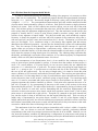
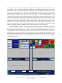
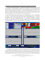
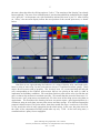
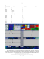
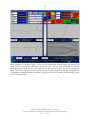
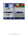
SpECS Vibrating String Experiment User’s Manual
Paul R. Woodward and B. Kevin Edgar
University of Minnesota
Laboratory for Computational Science & Engineering
Introduction:
The purpose of this experiment is to provide a computational laboratory for studying wave
propagation in one dimension. The computer program implements a discrete model of a vibrating
string by approximating the continuous, elastic system as a string of point masses joined together in
a straight line by massless springs. The concept of a point mass, that is of a mass concentrated
entirely at a single point, is obtained as the limit of a series of objects, all of the same mass, which
are denser and denser and smaller and smaller. Similarly, the massless spring is the limit of a
conceptual series of springs, all of the same length and all exerting the same force when stretched,
which have increasingly less and less mass. One can build in the laboratory excellent representations of the strings of masses joined by springs that come very close to the conceptual ideal of point
masses and massless springs (i.e. the masses are small and dense, while the springs are strong but
light). Such realizable physical models are the inspiration for the discretization of the continuous
string used by the computer simulation in this experiment. They should behave very much in
accordance with the results of the computations performed by this program. Checking that this is
indeed correct is left as an exercise for the ambitious user of this program.
The program assumes that the string has unit length (i.e. one inch, one foot, one meter, one
mile, or whatever) and that the string is fixed at its two end points. The tension along the string is
also assumed to be unity (see discussion of units below). The transverse displacement of the string
at any point along its length is computed by the program as a function of time and is displayed
dynamically as the computation proceeds. It is assumed that this transverse displacement, y,
which is set initially by the user, is always small. The force law used by the program, and
explained in the accompanying notes, does not make sense if this assumption is violated. The user
may enter transverse displacements that violate this restriction, but if this is done the results of the
computational experiment will be in error. Consequently, when the user enters large displacements, a message box pops up to give an appropriate warning.
This program can be used to investigate the behavior of either actual strings of masses joined
by springs or of continuous strings. In the first instance, the user selects a small number of point
masses, while in the second the user chooses a very large number of point masses. The behavior to
be expected when the number of point masses is small is explained in the notes for this experiment. Below, we will explain how to set up such an experiment to investigate the vibrations of 2
point masses. To compute a good approximation to the vibration of a continuous string, a large
number of point masses should be used. There is a trade-off here between the number of point
masses selected, and hence the quality of the result, and the cost of the computation in time (and in
memory consumed on the computer). A default value of 501 point masses is implemented in the
program, but users will find that the results they can obtain using, say, 2001 point masses are much
cleaner. The maximum number of point masses allowed by the program is 5001.
2
Just a Bit about How the Computer Model Works:
In order to understand properly the setup and working of the program, it is necessary to delve
just a little into its construction. The experiment program divides the approximated continuous
string into N+1 “grid cells.” Because the length of the string is unity, each of these grid cells has
a length of 1 / (N+1). The correspondence between these grid cells and the mechanical model
of point masses interconnected by springs is as follows. Each grid cell contains a single point mass
located at its center. Each cell also contains two massless springs, one on each side of the point
mass. Each of these springs is connected to the point mass, and on the other end each is connected
to the spring from the appropriate neighboring grid cell. Thus the mechanical model used by the
program is actually that of a series of point masses joined by massless springs, each of which
consists of two segments of equal length. This physical model may seem needlessly complex.
However, it allows the program to associate with each segment of the continuous string, that is,
with each grid cell, not only a mass and a tension but also a density. The density is of course the
mass per unit length. For a continuous string it is the density that, together with the tension,
determines the vibrational properties. Anyone who has looked inside a piano will understand this
fact. Thus, the concept of string density, which goes naturally with the concept of a grid cell,
applies when we are trying to approximate a continuous string. When we are computing the
vibrations of individual masses, as we do when the selected number of such masses, or grid cells, is
small, then the concept of string density gets a bit confusing. The vibrating string experiment has
this duality, and although it can lead to some confusion, it is an inherent property of computational
models, which are all by their fundamental nature discretized.
The consequences of our discretization, that is, of our model for the continuous string as a
series of point masses joined together by springs, is clearest when the number of these masses is
small. For a small number, N, of point masses, we can see most clearly why we subdivide the
string into N+1 rather than just N grid cells. The reason is that using springs of equal length, we
need N+1 springs to join N point masses to each other and also to two fixed walls. Consider
the case of just two point masses. For our string of length unity, it is natural to locate the point
masses a distance of 1/3 from each wall and also from each other. Then we have two point masses,
each with mass 1/3 if the string density is unity (if you think these masses should have the value ½,
see the discussion later in this section), and three springs of equal length. The remaining string
mass of 1/3 must be associated with point masses located in fixed positions on the walls. The
program represents this situation internally as follows. Each point mass represents the mass of its
grid cell, of length 1/3, by concentrating all that mass at the center of the section of the string
represented by the grid cell. The effect of the fixed walls is represented by placing a fictitious point
mass at the location of each wall, and by demanding that the transverse displacements and
velocities of these point masses must always vanish (their positions remain fixed). Each of these
point masses is associated with a grid cell too. That grid cell, centered on the wall, extends half
way into the region in front of and half way into the region behind the wall. Thus our string of
length unity is represented by two point masses, located 1/3 and 2/3 of the distance along its
length, and by three grid cells, one for each of these two point masses and half a cell for each of the
two fictitious, immovable point masses at each wall (the half-cells for the point masses at the walls
account for a third of the mass of the string in this case, see below).
The attachment of the first and last spring to immovable walls is what is called a boundary
condition. We can choose to treat this boundary condition specially, performing different
computations at the ends of our string of point masses than we do in its middle. However, we can
also treat this boundary condition by determining a configuration of point masses and springs at
and beyond each end of our string which will generate precisely the desired behavior at the ends of
SpECS Vibrating String Experiment User’s Manual
University of Minnesota, Laboratory for Computational Science & Engineering
Nov. 11, 1999
3
the string when we treat all point masses, both “real” and “fictitious,” in exactly the same way in
our program. This way of treating boundary conditions is encountered again and again in computational science. We can meet all necessary conditions by placing additional point masses on the
other sides of each of the walls. If the transverse displacement and velocity of such a fictitious
point mass just behind a wall is always set precisely equal to and of opposite sign from the
corresponding real point mass adjacent to the wall, then a moment’s thought leads to the
conclusion that the point mass located right at the wall will never experience any net force. The
two springs connected to it always pull equally and in opposite directions. The point mass at the
wall thus never moves, and the spring joining it to the first point mass in the series representing our
string might just as well be attached to an immovable wall as to this fictitious point mass. In our
program, we will have to set the positions and velocities of the fictitious point masses before each
time we update the state of our model vibrating string, but in this update computation we need
make no allowance for special treatment of any of the point masses, real or fictitious.
This construction is called a reflecting boundary condition, because we obtain the position
and velocity of the fictitious point mass behind the wall by reflecting the position and velocity of
the point mass near the wall just as in a mirror. We will see in our experiments that wave signals
that approach the wall will also be reflected by the wall. The behavior of these waves at the wall is
equivalent to the result we would obtain by letting the waves propagate right through the wall,
while the corresponding mirrored waves propagating toward the wall from the other side, moving
along the reflected, fictitious point masses and springs, emerge from the wall just as the original
waves disappear into it.
SpECS Vibrating String Experiment User’s Manual
University of Minnesota, Laboratory for Computational Science & Engineering
Nov. 11, 1999
4
The Vibrations of Two Point Masses Connected by Springs to Each Other and to Walls:
Enough about boundary conditions. To perform our experiment with two point masses and
three springs, we execute the program StringGUI.exe by clicking on it. This action brings up the
on-screen display. On the previous page, the screen display for the experiment is shown, where
the user has already entered a new value of 2 in the text window labeled “N Pt. Masses.” This
value of 2 has replaced the program’s default value of 501. We will set up one of the two “normal
modes” of oscillation for these two point masses, from which all other oscillatory modes may be
obtained by superposition, as explained in the notes for this experiment.
By default, the point mass on the left has an initial displacement of 0.01, a value that is
significant, yet still small compared to the length, unity, separating our two walls (i.e. the length of
our “string”). The point mass on the right, however, has a default displacement of 0, while we
would like to assign to it an initial displacement of -0.01. To make this adjustment, we can enter
the value “2” in the text box labeled “M Selected.” Equivalently, we can adjust the horizontal
scroll bar to the right of this label so that “2” appears in the “M Selected” window. After resetting
the displacement to -0.01, the on-screen display looks as shown below.
The change we have requested in the transverse displacement of the second point mass will
not be reflected in the graph until we click on the “Select” button. The user interface works by
letting us choose values for all the parameters associated with the selected point mass, namely its
transverse displacement, its transverse velocity, and its “density,” before we apply all these choices
by clicking on the “Select” button. If we wish to revise our choices, we can re-enter them and have
SpECS Vibrating String Experiment User’s Manual
University of Minnesota, Laboratory for Computational Science & Engineering
Nov. 11, 1999
5
the new values take effect by clicking again on “Select.” The meaning of the “density” has already
been explained. The mass of our selected point is just the selected density multiplied by the length
of its “grid cell.” In the present case, with unit density selected, this mass is just 1/3. After clicking
on “Select,” the on-screen display reflects the new position of the second point mass, as shown
below.
Note that we are approximating the behavior of a string of density unity and length unity,
hence a string of mass unity, by two point masses of mass 1/3 and three massless springs. These
masses do not seem to add up properly. The “missing” mass 1/3 is associated with the half grid
cells corresponding to the fictitious point masses that we are placing at the walls in order to
implement our boundary conditions. We want these fictitious point masses to be just like the real
ones, so that we do not have to treat them specially. This means that they must also have mass 1/3.
Thus our two “real” point masses constitute only 2/3 of the mass of the string we are using them to
approximate. This should not be alarming, because we cannot expect a good approximation of a
continuous string to result from just two point masses and three springs. If we had used instead the
program’s default value of 501 point masses, then these would sum up to a total mass of 501/502,
or very nearly the value of unity appropriate for the whole string. In this case, the point masses at
the walls in the computational model would make up only 1/502 of the total string mass, a
contribution that is pretty close to negligible.
SpECS Vibrating String Experiment User’s Manual
University of Minnesota, Laboratory for Computational Science & Engineering
Nov. 11, 1999
6
An aside on the issue of units:
It is worthwhile at this point to make a brief aside to discuss the issue of units. The program
does not use any inherent set of units. That is to say that the program manipulates numbers,
according to values entered by the user, and assumes that these numbers represent values in some
consistent set of units. The burden is on the user to keep track of the units, and to make sure that
all the values entered into the program are consistent in the units he or she is using. Thus it is the
user who decides whether the length of the string is one inch, one centimeter, one foot, one meter,
or, indeed, one light year. The density values entered by the user must represent values of mass
per unit of length, where that length is measured in the units used to interpret the unit length of the
string. If one uses the so-called cgs units (centimeters, grams, and seconds), then the string is one
centimeter long, and a density of unity must then mean a string of one gram per centimeter of
length. In this case, each of our two point masses would have a mass of 1/3 gram. The user cannot
change the value of the tension along the string, so it is important to note that if cgs units are being
used, then this tension is one dyne (a dyne is the force required to accelerate one gram by a
velocity increment of one centimeter per second every second). Similarly, the velocities entered by
the user must be consistently interpreted (that is, interpreted by the user in the way they will be
interpreted by the program). If cgs units are being used, then these velocities should be understood
to be given in centimeters per second. Note also that times are displayed by the program. When
cgs units are in use, these must be interpreted as seconds. As we will see presently, the program
can create velocities for the user, which gets around the difficulty of some figuring on the user’s
part. However, the program will display velocity values, and these are useless to the user unless he
or she knows their units in order to interpret this program output.
It is possible to write a program like this one without assuming a particular system of units,
because one can view the physical system as having a natural system of units all by itself. This is
because the results of the experiment can be scaled to arrive at equally valid results for strings of
different lengths. For example, if we wanted to obtain results for a string of 10 centimeters, we
would only have to multiply all the lengths produced by the program by a common factor of 10,
multiply all the times produced in the program output by this same scale factor, and multiply all
the masses by this factor as well. Because the velocities are all measured in lengths traversed per
unit of time, these would not be changed. The tension in the string, since it is a force, would also
be unchanged (the masses are now ten times larger and their separations are ten times greater, but
the time intervals are ten times greater as well, and these enter into the force raised to the second
power in the denominator). Thus the same numerical results of one string vibration experiment
hold when lengths are interpreted as centimeters, times as seconds, and masses as grams and also
when lengths are interpreted as meters, times as measured in numbers of 100 second intervals, and
masses as measured in numbers of 100 gram increments. In this case velocities would be
interpreted as numbers of meters that would be traversed in 100 second intervals, or, equivalently,
in centimeters per second. The new unit of force would be that required to accelerate a mass of
100 grams (or 0.1 kg) by a velocity increment of one meter per 100 seconds (or 0.01 m/sec) every
100 seconds. That is, this unit of force would still be one dyne. It is left as an exercise for the
reader to figure out how many Newtons (the unit of force in the mks system) this force of one dyne
is. This discussion may strike the reader as confusing, but it is worth thinking through, because it
allows each computer experiment to represent the behavior of a whole infinite class of similar
experiments. Each vibrating string experiment thus elucidates physical behavior that is in this sense
generic. In this way computers are used to discover modes of physical behavior of complex
systems that are general and are not tied to only a single, highly specific situation. In a sense, this is
related to the difference between computational science and computational engineering.
SpECS Vibrating String Experiment User’s Manual
University of Minnesota, Laboratory for Computational Science & Engineering
Nov. 11, 1999
7
Back to the initialization of the experiment with two point masses:
The on-screen display was shown above as it appears after clicking on the select button for the
second point mass. Note that default values have resulted in our setting the initial values of the
velocities of both point masses to zero. This corresponds to a physical experiment where we pull
the two masses to their initial positions, shown in the plot labeled “Displacement,” hold them
stationary there until, at time 0 (in the time system of this experiment), we let them both go. The
on-screen density plot shows that the “density” associated with each point mass is unity. This may
not be evident without putting a ruler up against the screen display. The text boxes at the left and
right under each of the plots on the display give the values of the minimum (left) and maximum
(right) values for the y-axis ranges in each plot. The x-axis, is of course always just as long as the
string, namely one length unit. This sort of display is fully adequate to give a visual impression of
the physical configuration, but it is not as quantitative as one might desire. To get full quantitative
detail, the user has only to manipulate the horizontal scroll bar next to the label “M Selected.” By
moving the scroll bar, or equivalently by entering the number of any desired point mass in the text
box labeled “M Selected,” the user can read the precise values of the position (point mass number),
density, velocity, and transverse displacement at that point along the string. For convenience, the
user can simply click in any of the three plot windows at the horizontal location where he or she
desires to obtain detailed numerical values of these quantities, and they will appear in the
appropriate text boxes. This can also be done while the experiment is running.
Setting the time to stop the experiment and to save and display results:
The experiment will begin, by definition, at time zero. We need to specify how long we want
it to run, and at what regular interval we would like its results to be saved for later visual or quantitative perusal. We have discussed earlier the time units for our experiment, that is, the units in
which we are to interpret the times that will be displayed in the window at the bottom center of the
on-screen display. To aid the user in choosing time intervals for saving output and for choosing
when to stop the experiment, a “period” is computed by the program. This period is the time that
it takes a small disturbance (a small transverse displacement of the string) to propagate along the
entire length of the string. This is, at least, the definition of the period in the case where we set the
density constant along the entire length of the string. In cases where the string density varies along
its length, this period is the time that such a disturbance would require to propagate along the
entire string if its density were everywhere equal to its density in the first grid cell, that is, at the leftmost end of the string. We will get a better understanding of this time interval, that we call one
period, presently. In the case of a string everywhere of density unity, this time interval is just unity
(i.e. one unit of time in whatever system we are using in the experiment).
We can tell the program when to stop the experiment by entering the number of periods we
want it to run in the text box to the left of the label “Periods to run.” The default value of 2
appears in this window followed by a decimal point to emphasize that we may enter any positive
number here, not just an integral number of periods. When the program reaches this point in the
experiment, it will pause and ask us if we want to continue (which would require entering a new,
larger value in the “Periods to run” text box and clicking on the ”continue” button) or if we want
to restart the run (by clicking on the “Restart” button and then on the “Begin” button), perhaps to
better observe something we may have missed. However, we don’t have to run the experiment
over again if we have saved data periodically during the run. To save data in this way, we need to
enter a value in the text box to the left of the “Plots per Period” label. The default is 20 plots per
period, and we can change this to any desired integer value. If we choose the default, the results of
our experiment are saved in the computer’s memory initially and after every time interval equal to
1/20 of a period. From this saved data, the program can generate plots of all the information from
SpECS Vibrating String Experiment User’s Manual
University of Minnesota, Laboratory for Computational Science & Engineering
Nov. 11, 1999
8
the experiment in its three plotting windows. Thus if we run the experiment for 10 periods, saving
40 “plots per period,” we will have 401 stored states of the system (of the vibrating string) to peruse
dynamically at the end of the experiment. We may access these stored states by manipulating the
vertical scroll bar in the center of the on-screen display. We may then click in any of the three
windows at a desired horizontal location, or we may manipulate the horizontal “M Selected” scroll
bar, in order to view detailed quantitative information in the various text windows on the display.
We may even generate a text file with long columns of numbers by clicking on the “Write Plotfile”
button. Such a text file can be used as input to a standard plotting package, or it can be perused for
detailed analysis by some user-generated computer program. In normal practice, we would not
expect to be generating such large text files, since the graphics of the on-screen display should give
us a very good feel for what is going on in our experiments.
Putting a title onto the on-screen display describing our experiment and printing the display:
Especially if we intend to capture and print the on-screen display for communicating the
results of our experiment to others, it is useful to generate a label for the experiment. Ample space
is provided for this purpose at the bottom of the display. We need only to click on the “Get Title”
button and to enter our title into the pop-up input box. It is a good idea to include in this title our
name, the date, and the purpose of the experiment. Of course, the entire display will be captured,
so there is no need to include redundant information. To get instructions on how to perform this
display capture, we can click on the button labeled “PRNT.” Because of Microsoft bugs in Visual
Basic, there is no proper way to simply print this display. Instead, we must click somewhere on the
“form” (not on a button) to make sure that it is “the active form,” and then press the “Alt” and
“PrntScrn” keys on the keyboard simultaneously. The display of our experiment will be captured
on the “clipboard,” from which it may be pasted into a Microsoft Word document, or otherwise be
packaged for output to a printer, or whatever. This is how the screen displays have been inserted
into this user’s manual.
Setting the display time interval and the number of the difference scheme:
Before we begin our experiment, we should set the value of a parameter that will control the
speed at which the experiment will run. In the text box to the left of the “msec per step” button,
we may enter the number of milliseconds that we wish to pass between successive computations
and accompanying plots on the screen. The default value of 5 msec, as shown in the screen as it
appears below, will let the experiment run at pretty much full speed. A value of 50 msec will not
slow it down very much, but a value of 500 msec will give only two display updates per second, a
rather graceful pace of change. To freeze the display and interrupt the computation, we can simply
click on the “pause” button. To resume the computation, we can click on “continue.” While the
experiment is paused, we can change some of its parameters, like the stop time and output interval,
and even the difference scheme we are using.
As is explained in detail in the notes accompanying this experiment, a number of different
numerical schemes are provided for use in this experiment. The default is to use scheme number
3. This scheme is the most robust, and in some respects it is also the least accurate. Scheme
number 4 is much more accurate in producing the time history of the transverse displacement, but
it achieves this accuracy at the cost of introducing very high frequency oscillations (for strings with
very many point masses) in the velocity distribution. Schemes 3 and 4 both keep high frequency
velocity oscillations at bay by introducing amplitude damping of the string vibration. In the case of
just 2 point masses that we are concerned with at present, this amplitude damping means that
either of these schemes will cause the point masses to stop vibrating after only several periods.
This behavior is easily observed by performing such an experiment. However, we will select
SpECS Vibrating String Experiment User’s Manual
University of Minnesota, Laboratory for Computational Science & Engineering
Nov. 11, 1999
9
scheme 2, which has the special property that it has no dissipation, so our point masses will
oscillate forever, as physical theory says that they should under ideal circumstances (i.e. no friction,
no losses involved with stretching and relaxation of the springs, etc.). We select scheme 2 by
entering a “2” in the “Scheme number” text box, as shown.
Saving and/or restoring a setup file:
We are now just about ready to begin our experiment. However, it might be useful at this
point, before any of our settings change as a result of running the experiment, to save our settings in
a disk file. We can do this by clicking on the “Write Setup” button. This allows us to specify a
file name into which all our settings will be written. At a later point, we could read this file in by
clicking on the “Read Setup” button and selecting this same file for input. This would cause all
our present settings to be restored. In this fashion, we can construct experiments that we may urge
our friends to perform, so that they can see and perhaps usefully comment upon some unexpected
phenomenon we might have discovered. For the curious, a listing of our setup file is as follows:
"NDifferenceScheme",
"NGridCells",
"WaveSpeed0",
"CourantNumber",
"YMax",
"YMin",
"RhoMax",
"RhoMin",
2
2
1
.5
.0105
-.0105
1.05
.95
SpECS Vibrating String Experiment User’s Manual
University of Minnesota, Laboratory for Computational Science & Engineering
Nov. 11, 1999
10
"VYMax",
"VYMin",
"Periods",
"NPlotsPerPeriod",
"NSelected",
""
"MSelected",
"Y",
0,
0,
1,
.01,
2,
-.01,
3,
0,
.01
-.01
10
40
2
"Rho",
1,
1,
1,
1,
"VY"
0
0
0
0
Running the experiment:
Running our experiment is now a breeze. We have only to click on the button labeled
“Begin.” When we get to the end that we specified, after 10 periods, a text box pops up to ask us if
we really want to plot all our stored states on top of each other on the display. For an experiment
involving lots of stored states and lots of point masses, this summary plotting could take quite some
time. It may not prove to be terribly valuable, and therefore the default response is to skip this
function. For our little experiment, the result of this summary plotting is shown above. Note that
because we saved 40 states per period, when they are all plotted, the screen is blackened. Clearly,
SpECS Vibrating String Experiment User’s Manual
University of Minnesota, Laboratory for Computational Science & Engineering
Nov. 11, 1999
11
this is not helpful. We can manually control the display of stored states as follows. First, we can
clear the plot windows by clicking on the “Clear” button at the top center of the display. Then we
can choose to display one plot or multiple plots at a time, by clicking on either the “Single” or the
“Multi” button, respectively. The plots that are displayed are then selected by manipulating the
vertical scroll bar at the center of the display, or by entering the number of a desired stored state in
the text window above this scroll bar.
The graphic in the lower right-hand plotting window that has now appeared at the completion
of the experiment takes a bit of explanation. This is a grayscale space-time plot showing at a single
glance the entire time development of the distribution of transverse displacement of the string. For
each of the 400 stored states, a thin horizontal slice of this picture has been created. In that thin
slice, the area corresponding to each grid cell (or to each point mass) has been shaded from black
to white according to the small or large value of the transverse displacement of that point mass at
that time in the experiment. Note that the half grid cells associated with the point masses that our
computational method places at the walls to implement the boundary conditions are shaded a
neutral gray at all times, since they always have transverse displacements of zero. Had we used
difference scheme 3 or 4, this space-time display would have revealed the damping of the
oscillation, because as we go up in this picture in that case, the color would go over to a nearly
uniform shade of middle-level gray. To understand the real usefulness of the space-time plot, and
also to understand the function of the “Wave” button, we must graduate to an experiment with
many point masses representing a continuous, vibrating string.
The Vibration of a Continuous String Plucked at the Center:
We will now consider an experiment intended to approximate the behavior of a continuous
string. We will therefore use a lot of point masses, namely 4001. This may seem like overkill, but
we want to obtain a truly clean result. We will study the vibration of a string that is plucked, as in a
harpsichord, rather than one that is struck, as in a piano. To keep things simple in this example, we
will pluck the string precisely at its center. That is why we choose to use 4001 point masses, or
grid cells, rather than the more natural number 4000. This will allow us to set the transverse
displacement of the point mass, or string element, numbered 2001 at a value of 0.01, leaving all
the velocities at zero and leaving the density of the string constant at a value of unity. To
accomplish this, we merely execute the vibrating string program, by clicking on its name,
StringGUI.exe, and then by entering the value 4001 into the “N Pt. Masses” text window.
Everything else comes automatically with the program’s defaults. The result of this experiment is
shown on the next page.
We can observe rather unusual behavior here, which is better seen by watching the experiment as it runs. The string snaps back, not all at once but beginning only at the center. The
stretched portions of the string at the sides remain stretched until signals have time to propagate
along the string from the center, carrying the vital information that the string has been released.
The velocity plots for these 2 periods, in which the string returns almost exactly to its original
position, lie almost on top of each other in pairs. To the extent that they do not lie directly on top
of each other, these velocity distributions indicate the dissipation of the numerical scheme. Even
with the selected huge number of point masses, 4001, the dissipation is visibly rounding the
corners of the sudden jumps in the velocity. For an “ideal” string, with no dissipation, these jumps
would be perfectly sharp. But of course, neither this numerical model nor any real string could
possibly do that. The vibration of this plucked string is a standing wave mode. This is clear from
the space-time plot in the panel at the bottom right in the on-screen display. This sort of standing
wave vibration should be familiar to anyone who has closely observed the strings of a guitar as the
SpECS Vibrating String Experiment User’s Manual
University of Minnesota, Laboratory for Computational Science & Engineering
Nov. 11, 1999
12
instrument is played. To see wave motion, we must not simply pluck the string; we must assign it
non-zero initial velocities as well as transverse displacements.
To create the initial conditions for a rightward traveling wave, we have only to set up our
desired initial transverse displacements, and then to click on the “Wave” button. Using the same
set of initial displacements as above, the result of running this new experiment is shown on the
next page.
We cannot get any idea of the wave propagation from the composite plots of the transverse
displacement, the velocity, and the density. Even watching these plots as the experiment runs, or
reviewing the time development after the fact by moving the vertical scroll bar through the series of
80 stored states does not give the impression of recognizable wave motion. This is because the
wave is constantly being superposed on its reflection from the fixed point at the one wall or the
other. However, the space-time plot at the bottom right in the on-screen display shown above
makes the wave propagation, and its reflection, immediately evident.
Some remarks about the significance of “selected” point masses (or grid cells):
In the section above, we skimmed over the significance of the “selected” grid cells, or point
masses. The user initializes the distributions of transverse displacement, transverse velocity, and
density by setting these properties for a set of selected grid cells. The program then interpolates
linearly between each pair of neighboring selected grid cells in order to set these same properties
for all the grid cells. This procedure makes it easy to set up the simple waveforms we have seen
above, but it makes it difficult to set up continuous, smooth waveforms, like sine waves. The only
SpECS Vibrating String Experiment User’s Manual
University of Minnesota, Laboratory for Computational Science & Engineering
Nov. 11, 1999
13
way in which such waves could be set up is for the user to generate, with some externally provided
program, a setup file containing an entry for every grid cell. This would not be terribly difficult, but
it would not be easy either. Nevertheless, there is nothing sacred about the sine wave, and one can
perform fascinating wave propagation experiments without them. As an example, consider the
case shown on the next page, which comes from initializing a rightward-traveling triangular wave
which propagates from a region of unit density into one of density 16.
The setup file for this experiment is as follows:
"NDifferenceScheme",
"NGridCells",
"WaveSpeed0",
"CourantNumber",
"YMax",
"YMin",
"RhoMax",
"RhoMin",
"VYMax",
"VYMin",
"Periods",
"NPlotsPerPeriod",
"NSelected",
3
4001
1
.5
.0105
-.0105
16.7525
.95
.110330125000003
-.1055525
6
40
17
SpECS Vibrating String Experiment User’s Manual
University of Minnesota, Laboratory for Computational Science & Engineering
Nov. 11, 1999
14
""
"MSelected",
0,
1,
1000,
1001,
1002,
1400,
1401,
1402,
1800,
1801,
1802,
2000,
2001,
2002,
2500,
2501,
2502,
4001,
4002,
"Y",
0,
0,
0,
0,
.000025,
.009975,
.01,
.009975,
.000025,
0,
0,
0,
0,
0,
0,
0,
0,
0,
0,
"Rho",
1,
1,
1,
1,
1,
1,
1,
1,
1,
1,
1,
1,
1,
1.03,
15.97,
16,
16,
16,
16,
"VY"
0
0
0
0
0
0
0
0
0
0
0
0
0
0
0
0
0
0
0
The display captured on the next page shows the waveform at the end of the experiment,
revealing the direct descendant of the original, isolated, single triangular signal (shown in the setup
screen above) as well as several reflected signals. The space-time display at the bottom right shows
SpECS Vibrating String Experiment User’s Manual
University of Minnesota, Laboratory for Computational Science & Engineering
Nov. 11, 1999
15
the propagation of all these signals, as they are transmitted and reflected again and again at the
linear ramp in string density indicated in the density plot. The first several waveforms, following
the experiment through the first wave transmission and reflection event, are shown on the next
page. This screen capture indicates the kind of analysis that can be done after the computation is
completed by clearing the plotting windows, clicking on the “Multi” button, and displaying several
successive stored states.
SpECS Vibrating String Experiment User’s Manual
University of Minnesota, Laboratory for Computational Science & Engineering
Nov. 11, 1999
16
SpECS Vibrating String Experiment User’s Manual
University of Minnesota, Laboratory for Computational Science & Engineering
Nov. 11, 1999