Download EDM Users Guide - Crystal Instruments India Private Limited

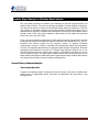
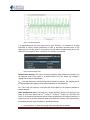
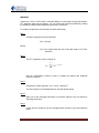
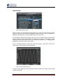
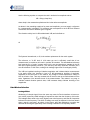
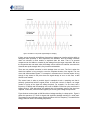
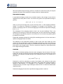
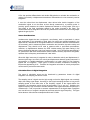
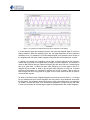
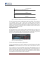
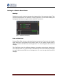
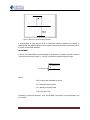
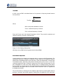
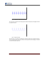
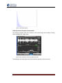
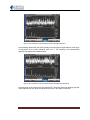
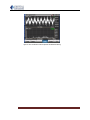
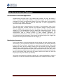
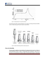
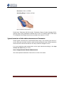
Vibration Data Collector
Signal Analysis
James Zhuge, Ph.D., President
Crystal Instruments Corporation
4633 Old Ironsides Drive, Suite 304
Santa Clara, CA 95054, USA
www.go-ci.com
(Part of VDC User’s Manual)
3/16/2009
COPYRIGHT © 2009 CRYSTAL INSTRUMENTS. ALL RIGHTS RESERVED.
PAGE 1
Dynamic Signal Analysis in Vibration Data Collector
The CoCo-80/90 provides two different user interfaces for Dynamic Signal Analyzer and
Vibration Data Collector. The style and settings are different to meet industrial conventions.
The user has the choice to enter one of the interfaces when system is powered on. The VDC
user interface is specifically designed for fast data collection operation and ease of use. A
professional user focused on research and development can open and use the DSA functions
instead of that of VDC. This section explains in detail about how the signals are processed
when CoCo runs in the VDC mode.
CoCo uses various different technologies of digital signal processing. Among them, the most
fundamental and popular technology is based on the Fast Fourier Transform (FFT). The FFT
transforms time domain signals into the frequency domain. To perform FFT-based
measurements, however, it helps to understand the fundamental issues and computations
involved. This Appendix describes some of the basic signal analysis computations, discusses
anti-aliasing and acquisition front end for FFT-based signal analysis, explains how to use
windowing functions correctly, explains some spectrum computations, and shows you how to
use FFT-based functions for some typical measurements. Users should be aware of the
subtle differences between a traditional dynamic signal analyzer and a vibration data collector
even though they all employ the same signal processing theory.
General Theory of Spectral Analysis
Time Domain Waveform
A typical time waveform signal in analog form from the sensor, such as an accelerometer,
velocity-meter or displacement probe, could take an appearance like that shown in the
following picture.
COPYRIGHT © 2009 CRYSTAL INSTRUMENTS. ALL RIGHTS RESERVED.
PAGE 2
Figure 1: Time Domain Waveform
In a digital instrument, much the same thing is seen. However, it is necessary in a digital
instrument to specify several parameters in order to accurately represent what is truly
happening in the analog world. It is important to tell the instrument what sample rate to use,
and how many samples to take. In doing this, the following are specified:
Figure 2: Parameter Setup in CoCo
Measurement Quantity: This field is required to determine what measurement quantity is to
be displayed. Even if the sensor is an accelerometer, the CoCo device can integrate it
digitally into velocity or displacement.
Fmax: This field defines the maximum frequency of interest for analysis. The sampling rate of
the analog/digital (A/D) digitizer will be determined based on this parameter.
Fmin: This is the low frequency cut-off filter that will be applied in the frequency domain for
spectral analysis.
Block Size/Spectral Lines: The block size is usually defined in blocks of two (binary) to the
10
11
12
power of 10 or more. (Block size of 2 is 1024, 2 is 2048, 2 is 4096, etc.) The block size
and Fmax will determine the total time period of each sampling block for frequency analysis. A
larger block size for the same frequency band will increase the accuracy of the measurement.
Immediately after the signal is digitized, it will also go through:

Low pass filters - to eliminate any high frequencies that are not wanted
COPYRIGHT © 2009 CRYSTAL INSTRUMENTS. ALL RIGHTS RESERVED.
PAGE 3

High pass filters - to eliminate DC and low frequency noise that are not wanted
Additionally, the integration of the signal provides velocity or displacement from an
accelerometer or a displacement from a velocity pickup. Traditional signal analyzers have a
drawback of dynamic range in the digital domain and some argue that the analog integration
is superior to that of digital. The situation is greatly improved due to the very high dynamic
range technology in the CoCo. With more than 130dB dynamic range in the front end, digital
integration can achieve excellent accurate results.
The Fourier Transform
CoCo fully utilizes FFT frequency analysis methods and various real time digital filters to
analyze measurement signals. The Fourier Transform is used to convert quantities amplitude
vs time in the time domain (time waveform) to amplitude vs frequency in the frequency
domain (FFT spectrum), usually derived from the Fourier integral of a periodic function when
the period grows without limit, often expressed as a Fourier transform pair. In the classical
sense, a Fourier transform takes the form of:
∞
𝑋 𝑓 =
𝑥 𝑡 𝑒 −𝑗 2𝜋𝑓𝑡 𝑑𝑡
−∞
Where:
x(t)
continuous time waveform
f
frequency variable
j
complex number
X(f)
Fourier transform of x(t)
As the theory of Jean Baptiste Fourier states: All waveforms, no matter how complex, can be
expressed as the sum of sine waves of varying amplitudes, phase, and frequencies. In the
case of rotating machinery vibration, this is most certainly true. A machine's time waveform is
predominantly the sum of many sine waves of differing amplitudes and frequencies. The
challenge is to break down the complex time-waveform into the components from which it is
made.
Mathematically the Fourier Transform is defined for all frequencies from negative to positive
infinity. However, the spectrum is usually symmetric and it is common to only consider the
single-sided spectrum which is the spectrum from zero to positive infinity. For discrete
sampled signals, this can be expressed as:
𝑁−1
𝑥 𝑘 𝑒 −𝑗 2𝜋𝑘𝑛 /𝑁
𝑋 𝑘 =
𝑛 =0
COPYRIGHT © 2009 CRYSTAL INSTRUMENTS. ALL RIGHTS RESERVED.
PAGE 4
Where:
x(k)
samples of time waveform
n
running sample index
N
total number of samples or “frame size”
k
finite analysis frequency, corresponding to “FFT bin
centers”
X(k)
discrete Fourier transform of x(k)
In CoCo, a Radix-2 DIF FFT algorithm is used, which requires that the total number of
samples must be a power of 2 (total number of samples in FFT = 2m , where m is an integer).
The Fourier Transform assumes that the time signal is periodic and infinite in duration. When
only a portion of a record is analyzed the record must be truncated by a data window to
preserve the frequency characteristics. A window can be expressed in either the time domain
or in the frequency domain, although the former is more common. To reduce the edge effects,
which cause leakage, a window is often given a shape or weighting function. For example, a
window can be defined as:
w(t) = g(t)
=0
-T/2 < t < T/2
elsewhere
where g(t) is the window weighting function and T is the window duration.
The data analyzed, x(t) are then given by:
x(t) = w(t) x(t)’
where x(t)’ is the original data and x(t) is the data used for spectral analysis.
A window in the time domain is represented by a multiplication and hence, is a convolution in
the frequency domain. A convolution can be thought of as a smoothing function. This
smoothing can be represented by an effective filter shape of the window; i.e., energy at a
frequency in the original data will appear at other frequencies as given by the filter shape.
Since time domain windows can be represented as a filter in the frequency domain, the time
domain windowing can be accomplished directly in the frequency domain.
Because creating a data window attenuates a portion of the original data, a certain amount of
correction has to be made in order to get an un-biased estimation of the spectra. In linear
spectral analysis, an Amplitude Correction is applied.
COPYRIGHT © 2009 CRYSTAL INSTRUMENTS. ALL RIGHTS RESERVED.
PAGE 5
Spectrum
A spectrum in CoCo in VDC mode is calculated based on a few steps including data window,
FFT, amplitude scaling and averaging. You can extract the harmonic amplitude by reading
the amplitude values at those harmonic frequencies in a spectrum.
To compute the spectrum, the instrument will follow these steps:
Step 1
A window is applied to the time waveform:
x(k) = w(k) x(k)’
Where:
x(k)’ is the original data and x(k) is the data used for a Fourier
transform.
Step 2
The FFT is applied to x(k) to compute Sx:
𝑁−1
𝑥 𝑘 𝑒 −𝑗 2𝜋𝑘𝑛 /𝑁
𝑆𝑥 =
𝑛 =0
Next the “periodogram” method is used to compute the spectra with amplitude
correction using Sx.
Step 3
*
Calculate the “Power Spectrum” Sxx = Sx Sx / (AmpCorr)
2
The factor AmpCorr is calculated based on the data window shape.
Step 4
Apply one of the averaging techniques to the power spectrum Sxx (see below for
averaging techniques)
Step 5
Finally, take the square-root of the averaged power spectrum to get final spectrum
result.
COPYRIGHT © 2009 CRYSTAL INSTRUMENTS. ALL RIGHTS RESERVED.
PAGE 6
Spectrum Type
Figure 3: Display Preference Setup
Now we come to a confusing part about the spectrum of a signal. With the same time domain
signal, the spectrum can actually be displayed in different values. This is controlled by a
parameter, spectrum type, set in the Display Preference on the CoCo.
The motivation of doing so is that people may want to look at different aspect of the spectrum
and give different physical interpretation to the original time signals. For example, from the
spectrum the user may wants to know the frequency component at 1X rotating speed,
represented in its Peak, Peak to Peak or RMS.
To give a practical example, a 100Hz sine wave with roughly 1.0 peak in/s is fed into the
CoCo system. The time waveform is shown below:
Figure 4: Time Domain Waveform in CoCo
A very common reading will show a spectrum peak at 100Hz with a peak value reading
1.0208 in in/s (Peak)
COPYRIGHT © 2009 CRYSTAL INSTRUMENTS. ALL RIGHTS RESERVED.
PAGE 7
Figure 5: FFT Spectrum in CoCo, in/s Peak
If somebody is interested in the RMS value of this frequency component, he can change the
spectrum type to RMS, then the display value will be changed to 0.7218.
Figure 6: FFT Spectrum in CoCo, in/s RMS
Similarly, the user can look at Peak to Peak, vDB(SI) and vDB(US) of the spectral peak.
Now let’s introduce the concept of dB.
Most often, spectra are shown in the logarithmic unit decibels (dB). Using this unit of measure,
it is easy to view wide dynamic ranges; that is, it is easy to see small signal components in
the presence of large ones. The decibel is a unit of ratio and is computed as follows.
dB = 10log10 (PowerPref)
where Power is the measured power and Pref is the reference power.
COPYRIGHT © 2009 CRYSTAL INSTRUMENTS. ALL RIGHTS RESERVED.
PAGE 8
Use the following equation to compute the ratio in decibels from amplitude values:
dB = 20log10 (AmplAref)
where Ampl is the measured amplitude and Aref is the reference amplitude.
As shown in the preceding equations for power and amplitude, you must supply a reference
for a measurement in decibels. This reference then corresponds to the 0 dB level. Different
conventions are used for different types of signals.
The vibration velocity level in dB is abbreviated VdB, and is defined as:
Or
The Systeme Internationale, or SI, is the modern replacement for the metric system.
The reference, or "0 dB" level of 10-9 meter per sec is sufficiently small that all our
measurements on machines will result in positive dB numbers. This standardized reference
level uses the SI, or "metric," system units, but it is not recognized as a standard in the US
and other English-speaking countries. (The US Navy and many American industries use a
zero dB reference of 10-8 m/sec, making their readings higher than SI readings by 20 dB.)
The VdB is a logarithmic scaling of vibration magnitude, and it allows relative measurements
to be easily made. Any increase in level of 6 dB represents a doubling of amplitude,
regardless of the initial level. In like manner, any change of 20 dB represents a change in
level by a factor of ten. Thus any constant ratio of levels is seen as a certain distance on the
scale, regardless of the absolute levels of the measurements. This makes it very easy to
evaluate trended vibration spectral data; 6 dB increases always indicate doubling of the
magnitudes.
Data Window Selection
Leakage Effect
Windowing of a simple signal, like a sine wave may cause its Fourier transform to have nonzero values (commonly called leakage) at frequencies other than the frequency of this sine.
This leakage effect tends to be worst (highest) near sine frequency and least at frequencies
farthest from sine frequency. The effect of leakage can easily be depicted in the time domain
when a signal is truncated. As shown in the picture, after data windowing, truncation has
distorted the time signal significantly, hence causing a distortion in its frequency domain.
COPYRIGHT © 2009 CRYSTAL INSTRUMENTS. ALL RIGHTS RESERVED.
PAGE 9
Figure 7. Illustration of a non-periodic signal resulting from sampling
If there are two sinusoids, with different frequencies, leakage can interfere with the ability to
distinguish them spectrally. If their frequencies are dissimilar, then the leakage interferes
when one sinusoid is much smaller in amplitude than the other. That is, its spectral
component can be hidden or masked by the leakage from the larger component. But when
the frequencies are near each other, the leakage can be sufficient to interfere even when the
sinusoids are equal strength; that is, they become undetectable.
There are two possible scenarios in which leakage does not occur. The first is when the
whole time capture is long enough to cover the complete duration of the signals. This can
occur with short transient signals. For example in a hammer test, if the time capture is long
enough it may extend to the point where the signal decays to zero. In this case, a data
window is not needed.
The second case is when a periodic signal is sampled at such a sampling rate that is
perfectly synchronized with the signal period, so that with a block of capture, an integer
number of cycles of the signal are always acquired. For example, if a sine wave has a
frequency of 1000Hz and the sampling rate is set to 8000Hz. Each sine cycle would have 8
integer points. If 1024 data points are acquired then 128 complete cycles of the signal are
captured. In this case, with no window applied you still can get a leakage-free spectrum.
Figure 8 shows a sine signal at 1000 Hz with no leakage resulting in a sharp spike. Figure 9
shows the spectrum of a 1010 Hz signal with significant leakage resulting in a wide peak.
The spectrum has significant energy outside the narrow 1010 Hz frequency. It is said that the
energy leaks out into the surrounding frequencies.
COPYRIGHT © 2009 CRYSTAL INSTRUMENTS. ALL RIGHTS RESERVED.
PAGE 10
Figure 8. Sine spectrum with no leakage.
Figure 9. Sine spectrum with significant leakage.
Uniform window (rectangular)
𝒘 𝒌 = 𝟏. 𝟎
Uniform is the same as no window function.
Hann window
𝒘 𝒌 = 𝟎. 𝟓 − 𝟎. 𝟓 𝐜𝐨𝐬(
𝟐𝝅𝒌
)
𝑵−𝟏
Flattop window
COPYRIGHT © 2009 CRYSTAL INSTRUMENTS. ALL RIGHTS RESERVED.
PAGE 11
𝟐𝝅𝒌
𝟒𝝅𝒌
𝟔𝝅𝒌
+ 𝟏. 𝟐𝟗 𝐜𝐨𝐬
− 𝟎. 𝟑𝟖𝟖 𝐜𝐨𝐬
𝑵−𝟏
𝑵−𝟏
𝑵−𝟏
𝟖𝝅𝒌
+ 𝟎. 𝟎𝟑𝟐 𝐜𝐨𝐬
𝒇𝒐𝒓 𝒌 = 𝟎~𝑵 − 𝟏
𝑵−𝟏
𝒘 𝒌 = 𝟏 − 𝟏. 𝟗𝟑 𝐜𝐨𝐬
The term "Hanning window" is sometimes used to refer to the Hann window, but is
ambiguous as it is easily confused with Hamming window.
If a measurement can be made so that no leakage effect will occur, then do not apply any
window (in the software, select Uniform.). As discussed before, this only occurs when the
time capture is long enough to cover the whole transient range, or when the signal is exactly
periodic in the time frame.
If the goal of the analysis is to discriminate two or multiple sine waves in the frequency
domain, spectral resolution is very critical. For such application, choose a data window with
very narrow main slope. Hanning is a good choice. In general, we recommend Hanning
window in VDC applications.
When you are extremely sensitive to the accuracy of peak estimation at certain frequency,
choose Flattop window. It will give you the best estimation for the frequency components
measured at a rotating machine or reciprocating machine.
Averaging Techniques
Averaging is widely used in spectral measurements. It improves the measurement and
analysis of signals that are purely random or mixed random and periodic. Averaged
measurements can yield either higher signal-to-noise ratios or improved statistical accuracy.
Typically, three types of averaging methods are available in DSA products. They are:
Linear Averaging, Exponential Averaging, and Peak-Hold
Linear Averaging
In linear averaging, each set of data (a record) contributes equally to the average. The value
at any point in the linear average in given by the equation:
𝐴𝑣𝑒𝑟𝑎𝑔𝑒𝑑 =
𝑆𝑢𝑚 𝑜𝑓 𝑅𝑒𝑐𝑜𝑟𝑑𝑠
𝑁
N is the total number of the records. The advantage of this averaging method is that it is
faster to compute and the result is un-biased. However, this method is suitable only for
analyzing short signal records or stationary signals, since the average tends to stabilize. The
contribution of new records eventually will cease to change the value of the average.
Usually, a target average number is defined. The algorithm is made so that before the target
average number reaches, the process can be stopped and the averaged result can still be
used.
COPYRIGHT © 2009 CRYSTAL INSTRUMENTS. ALL RIGHTS RESERVED.
PAGE 12
When the specified target averaging number is reached, the instrument usually will stop the
acquisition and wait for the instruction for another collection of data acquisition.
Exponential Averaging
In exponential averaging, records do not contribute equally to the average. A new record is
weighted more heavily than old ones. The value at any point in the exponential average is
given by:
𝑦 𝑛 = 𝑦 𝑛 − 1 ∗ 1 − 𝛼 + 𝑥[𝑛] ∗ 𝛼
where 𝑦 𝑛 is the nth average and 𝑥[𝑛] is the nth new record.  is the weighting coefficient.
Usually  is defined as 1/(Number of Averaging). For example in the instrument, if the
Number of Averaging is set to 3 and the averaging type is selected as exponential averaging,
then 𝛼 = 1/3
The advantage of this averaging method is that it can be used indefinitely. That is, the
average will not converge to some value and stay there, as is the case with linear averaging.
The average will dynamically respond to the influence of new records and gradually ignore
the effects of old records.
Exponential averaging simulates the analog filter smoothing process. It will not reset when a
specified averaging number is reached.
The drawback of the exponential averaging is that a large value may embed too much
memory into the average result. If there is a transient large value as input, it may take a long
time for y[n] to decay. On the contrary, the contribution of small input value of x[n] will have
little impact to the averaged output. Therefore, exponential average fits a stable signal better
than a signal with large fluctuations.
Peak-Hold
This method, technically speaking, does not involve averaging in the strict sense of the word.
Instead, the “average” produced by the peak hold method produces a record that at any point
represents the maximum envelope among all the component records. The equation for a
peak-hold is
𝑦 𝑛 = MAX N−1
j=0 𝑥[𝑛 − 𝑗]
Peak-hold is useful for maintaining a record of the highest value attained at each point
throughout the sequence of ensembles. Peak-Hold is not a linear math operation therefore it
should be used carefully. It is acceptable to use Peak-Hold in auto-power spectrum
measurement but you would not get meaningful results for FRF or Coherence measurement
using Peak-Hold.
Peak-hold averaging will reset after a specified averaging number is reached.
COPYRIGHT © 2009 CRYSTAL INSTRUMENTS. ALL RIGHTS RESERVED.
PAGE 13
Overlap Processing
To increase the speed of spectral calculation, overlap processing can be used to reduce the
measurement time. The diagram below shows how the overlap is realized.
Figure 10. Illustration of overlap processing.
As shown in this picture, when a frame of new data is acquired after passing the Acquisition
Mode control, only a portion of the new data will be used. Overlap calculation will speed up
the calculation with the same target average number. The percentage of overlap is called
overlap ratio. 25% overlap means 25% of the old data will be used for each spectral
processing. 0% overlap means that no old data will be reused.
Overlap processing can improve the accuracy of spectral estimation. This is because when a
data window is applied, some useful information is attenuated by the data window on two
ends of each block. However, it is not true that the higher the overlap ratio the higher the
spectral estimation accuracy. For Hanning window, when the overlap ratio is more than 50%,
the estimation accuracy of the spectra will not be improved.
Another advantage to apply overlap processing is that it helps to update the display more
quickly.
Built-In Digital Integration And Filtering
Introduction to Digital Integration
Ideally, a measurement is made using a sensor that directly measures the desired quantity.
For example an accelerometer should be used to measure acceleration, a laser velocimeter
or velocity pickup should be used to measure velocity and a linear voltage displacement
transducer (LVDT) should be used to measure position. However since position, velocity and
acceleration are related by the time derivatives it is possible to measure an acceleration
signal and then compute the velocity and position by mathematical integration. Alternatively
COPYRIGHT © 2009 CRYSTAL INSTRUMENTS. ALL RIGHTS RESERVED.
PAGE 14
you can measure position and compute velocity and acceleration by differentiating. The
integration can be performed at the analog hardware level or at the digital level.
The CoCo provides a means to digitally integrate or double integrate the incoming signals.
The integration module fits into the very first stage after data is digitized, as shown below:
Analog
Signal
Conditioning
A/D
Converter
(Optional)
High-Pass Filter
and Integration
Data
Conditioning
Spectral
Analysis
CoCo
Figure 11: Signal Processing Sequence in CoCo
There are several issues to address in such implementation:
1. The integration and double integration algorithm has to be accurate enough and it
must find a way to reduce the effects of a DC offset. A tiny initial value, offset in the
measurement or temperature drift before the integration, may result in a huge value
after single or double integration. This DC effect can be removed using a high-pass
filter.
2. The initial digital signal must have a high signal to noise ration and high dynamic
range. The integration process in essence will reduce the high frequency energy and
elevate the low frequency components. If the original signals do not have good
signal to noise ratio and dynamic range, the signals after integration and double
integration will have too much noise to use. The noise will corrupt the integrated
signal.
3. The instrument must be able to set two different engineering units: one engineering
unit for the input transducer and a second engineering unit after the integration. For
example, first the instrument must provide a means to set the sensitivity of the sensor,
say 100mV/g in acceleration. After the double integration the instrument must have
the means to set the engineering unit to a unit that is compatible with the integration
such as mm of displacement.
The CoCo instrument handles these three issues effectively so you can get reliable velocity
or displacement signals from the acceleration measurement, or displacement signals from
the velocity measurement. The CoCo hardware has a unique design to provide 130dB
dynamic range in its front-end measurement. The signals with high dynamic range will create
better results after digital integration.
Since such built-in integration is conducted in the time domain before any other data
conditioning or spectral analysis, the time streams generated after the digital integration can
be treated in the same way as other time streams. They can be analyzed or recorded.
COPYRIGHT © 2009 CRYSTAL INSTRUMENTS. ALL RIGHTS RESERVED.
PAGE 15
CoCo also provides differentiation and double differentiation to calculate the acceleration or
velocity from velocity or displacement transducers. Differentiation is not as commonly used as
integration.
It must be noticed that the displacement value derived after double integration of the
acceleration signal is not the same as that directly measured by a proximity probe. A
proximity probe measures the relative displacement between a moving object (such as a
rotor shaft) to the fixed coordinates seated by the probe (mounted to the case). The
accelerometer and its integration value can only measure the movement of the moving object
against the gravity field.
Sensor Considerations
Accelerometer signals that are non-dynamic, non-vibratory, static or quasi-static in nature
(low acceleration of an automobile or flight path of a rocket) are typically integrated in the
digital domain, downstream of the signal conditioner. Piezoelectric and IEPE accelerometers
are commonly used to measure dynamic acceleration and, therefore, dynamic velocity and
displacement. They should not be used to measure static or quasi-static accelerations,
velocities, or displacements because the IEPE includes analog high pass filtering in the
sensor conditioning that cuts out any low frequency signal. At low frequencies approaching 0
Hz, piezoelectric and IEPE accelerometers cannot, with the accuracy required for integration,
represent the low frequency accelerations of a test article.
When this slight inaccuracy is integrated in order to determine velocity and displacement, it
becomes quite large. As a result, the velocity and displacement data are grossly inaccurate. A
piezoresistive or variable-capacitance accelerometer is a better choice for low frequency
signals and for integration. These types of sensors measure acceleration accurately at
frequencies approaching 0 Hz. Therefore the integration calculation of velocity and position
can be used to produce accurate results.
Calculation Errors in Digital Integration
Two types of calculation errors can be introduced by parameters chosen for digital
integration: low sampling rate and DC offset.
The sampling rate of a signal must be high enough so that the digital signal can accurately
depict the analog signal shape. According to the Nyquist sampling theorem as long as the
sampling speed is more than twice of the frequency content of the signals before the
integration, the integration results should be acceptable. This is not true. Satisfying the
Nyquist frequency only ensures an accurate estimate of the highest detectable frequency of a
measurement. It will not provide an accurate representation of the signal shape. Integration
error can still occur of a signal is sampled at more than twice the signal frequency. The figure
below shows a 1kHz sine wave sampled at 8kHz and 5.12kHz.
COPYRIGHT © 2009 CRYSTAL INSTRUMENTS. ALL RIGHTS RESERVED.
PAGE 16
Figure 12. A 1 kHz sine wave sampled at 8 kHz (top) and also sampled at 5.12 kHz (bottom).
It is clear that the higher the sampling frequency, the closer this digitized signal is to the true
analog waveform. When the sampling rate is low, the digital integration will have significant
calculation error. For example the 5.12 kHz sampled signal is not symmetric about 0 volts so
the integration will drift and a double integration may grow with accumulated error very fast.
In general, you should use a sampling rate at least 10 times higher than the frequency
content that is of interest in the signal when you apply numerical integration. (For example, a
motor at 3600 RPM is driving a machine through a gear box which has a 3:1 reduction gear
with 36:12 gear teeth. To detect the gear mesh frequency, the motor speed of 60 Hz is
multiplied by the number of teeth to get the gear mesh frequency of 2160 Hz. To detect
problems in the gearbox it is necessary to sample at 2.16 kHz or higher.) Think of trying to
draw a single sine wave using points on a graph. It will be much more clear with 10 points or
more than with only two.
DC offset is the second type of digital integration error and can be more severe. It is caused
by any measurement error before integration and may result in huge amplitude errors after
the integration. The illustration below shows how a small measurement error in acceleration
will create a constant DC offset in the acceleration integrated to compute velocity and result
in a drift and eventually an infinitely large magnitude of displacement after double integration.
COPYRIGHT © 2009 CRYSTAL INSTRUMENTS. ALL RIGHTS RESERVED.
PAGE 17
Displacement
Velocity
Acceleration
Figure 13. A small error in acceleration results in a DC offset in velocity and a huge drift in displacement.
Of course, the computed velocity and displacement signals are unrealistic. They are artifacts
of the integration errors. In order to remove such a problem caused by inaccurate
measurement and digital integration, a high pass filter can be applied before or after the
integration. It should be noted that the high-pass filter will distort the waveform shape to some
extent because it alters the low frequency content of the signal. However this effect must be
tolerated if numerical integration is used.
Digital High-Pass Filter
The most effective way to remove the DC drift effect as described above is to apply a high
pass digital filter to the continuous time streams. In CoCo, a unique algorithm is realized so
that even the data is sampled at high rate, the high pass filter can still achieve very low cutoff
frequency. The high pass filter parameter can be entered in the channel table.
Figure 14: CoCo Input Channel Setup Table
The filter cutoff frequency is specified at -3dB attenuation.
To remove unwanted signals at or near DC, please set up the cutoff frequency of the digital
high-pass filter as high as possible as long as it won’t chop off useful frequency content of
your interest.
To give an example, if you are not interested in any frequency less than 20Hz, then you can
set the cutoff frequency to approximately 10Hz. With this setting, the amplitude attenuation at
20Hz will be less than 1dB. (Typically, the lowest frequency of interest on rotating machinery
will be one half the running speed of the machine. If the high pass filter is set to one third the
running speed, the half order vibration will still be detectable.)
COPYRIGHT © 2009 CRYSTAL INSTRUMENTS. ALL RIGHTS RESERVED.
PAGE 18
Readings in a Vibration Data Collector
Readings
Readings are overall values that represent the characteristics of the measured signals. They
are either calculated from time waveform or frequency spectrum. In CoCo these readings can
be displayed individually or together with the waveform or spectrum.
Figure 15: Onsite Measurement Display
Peak and Peak-Peak
Peak and Peak-Peak values are calculated from the time waveform. Peak value is the largest
signal level seen in a waveform over a period of time. For sine signals, the peak value is
always 1.414 times the RMS value of the signal level. For non-sine signals, this formula will
not apply.
The Peak-Peak value is the difference between the maximum and minimum signal levels
over a period of time. For a pure sine wave, the Peak-Peak level is two times the peak signal
level and 2.828 times the RMS value of the signal level. For a non-sine signal this formula will
not apply.
COPYRIGHT © 2009 CRYSTAL INSTRUMENTS. ALL RIGHTS RESERVED.
PAGE 19
peak
Peak-peak
Figure 16: Illustration of Time Domain Peak, Peak-Peak
If accelerometer is used and the Peak or Peak-Peak reading is displayed for velocity or
displacement, the digital integration will be applied to the time waveform continuously before
the Peak or Peak-Peak detection.
Overall RMS
In CoCo, the overall RMS is calculated based on the spectrum in frequency domain across all
of the effective frequency range, i.e, from DC to maximum analysis frequency range.
fs*0.45
overallrms 

Power ( f )
0
BW
Where:
BW = noise power bandwidth of window
Fa = analysis frequency band
Fs = sampling frequency band
0.45 = the ratio of Fa/
According to “Parseval's theorem”, such overall RMS is equivalent to that calculated in the
time domain.
COPYRIGHT © 2009 CRYSTAL INSTRUMENTS. ALL RIGHTS RESERVED.
PAGE 20
True RMS
In CoCo, the true RMS is calculated based on the spectrum in frequency domain between
Fmin and Fmax.
f max
TrueRms 
 Power ( f )
f min
BW
Where:
BW = noise power bandwidth of window
Fmax = maximum frequency of interest
Fmin = minimum frequency of interest
Fmax and Fmin are set in the Analysis Parameters in CoCo. They control the maximum and
minimum frequency of interest, as shown below:
Figure 17: CoCo Display, Setting Fmax
Obviously, the true RMS will be no greater than the Overall RMS.
Demodulation Spectrum
A useful technique for measuring and analyzing data is a process called Demodulation. The
demodulation process is effective for detection of high frequency low amplitude repetitive
patterns that lie embedded within the time waveform. These are characteristic of certain types
of mechanical faults, particularly rolling element bearing faults such as inner or outer race
cracks and spalls that make a clicking or ringing tone as the rolling elements pass over the
fault. Demodulation is useful as an early warning device, as it detects bearing tones before
they are visible in a normal spectrum. As the fault progresses towards failure, the frequencies
will spread out and appear more as an increase in the “noise floor” of the FFT spectrum as
the amplitude increases.
The process works by extracting the low amplitude, high frequency impact signals and then
tracing an 'envelope' around these signals to identify them as repetitions of the same fault.
COPYRIGHT © 2009 CRYSTAL INSTRUMENTS. ALL RIGHTS RESERVED.
PAGE 21
The resulting spectrum, with the low frequency data removed, will now clearly show the high
frequency impact signals and harmonics.
The high frequency signals that demodulation aims to extract are do not travel well through
large structures, therefore extra care must be taken to ensure the accelerometer is setup
correctly. Ensure that:

The accelerometer is mounted close to the fault source with the shortest direct path
through the structure to the accelerometer.

The accelerometer is well coupled, using either stud mounting or a very strong
magnet on bare metal. A handheld probe or stinger is not recommended.

The accelerometer mounting is consistent between visits. If not, a trend plot of overall
RMS values will be meaningless.
The demodulation process can be graphically described in the following flow chart:
Figure 18: Demodulation Process Flow Chart
Below is a depiction of an acceleration time waveform with a repetitive high frequency
component. Because of the large difference in amplitude and frequency, a very low amplitude
high frequency signal could be overlooked during routine vibration analysis.
Figure 19: Acceleration Time Waveform with Fault
The high-pass filter removes the low frequency component of the signal, below:
COPYRIGHT © 2009 CRYSTAL INSTRUMENTS. ALL RIGHTS RESERVED.
PAGE 22
Figure 20: Acceleration Time Waveform after High Pass Filter
The next step in the process is enveloping which lowers the frequency of the signal to that of
the repetitive element.
Figure 21: Signal after Enveloping
The final step is to process the resulting time waveform signal into a frequency spectrum.
Since the signal has been altered by removal of low frequencies and enveloping, it is referred
to as the Demodulated Spectrum.
COPYRIGHT © 2009 CRYSTAL INSTRUMENTS. ALL RIGHTS RESERVED.
PAGE 23
Figure 22: Demodulated Spectrum
A Bearing Detection Example of Demodulation
The following examples show CoCo screens in VDC mode being used to analyze a rolling
element bearing with a slight defect.
Figure 23: CH1 Time Waveform and FFT with slight bearing defect
The following is the same signal with the demodulation spectrum on the lower trace:
COPYRIGHT © 2009 CRYSTAL INSTRUMENTS. ALL RIGHTS RESERVED.
PAGE 24
Figure 24: CH1 Time Waveform and Demodulation Spectrum with slight bearing defect
As the bearing deteriorates, the defect typically becomes larger and generates a wider range
of frequencies as the rolling elements pass over it. The following is the demodulation
spectrum with slightly deteriorated bearing:
Figure 25: CH1 Time Waveform and Demodulation Spectrum with slightly deteriorated bearing
As can be seen in the screen below, the standard FFT spectrum shows the relatively high first
order amplitude but only shows an elevated noise floor in the higher frequencies.
COPYRIGHT © 2009 CRYSTAL INSTRUMENTS. ALL RIGHTS RESERVED.
PAGE 25
Figure 26: CH1 Time Waveform and FFT Spectrum with deteriorated bearing
COPYRIGHT © 2009 CRYSTAL INSTRUMENTS. ALL RIGHTS RESERVED.
PAGE 26
Using Accelerometers and Tachometer
Accelerometers for Industrial Applications
Accelerometers are widely used in the vibration data collection. By using the feature of
CoCo’s very high dynamic range (130dB), the acceleration signals can also be accurately
integrated into velocity and displacement signals. There are a wide range of accelerometers
to choose in the market. Many of them are IEPE mode. In most of applications we
recommend using IEPE accelerometers.
There are three types of accelerometers in the market: (1). accelerometers used for costsensitive market such as PDAs, electronic toys, automotive airbags or laptop computers.
These are MEMS based sensors that cost a few dollars each. They do not fall into our
categories. (2). The accelerometers used for testing and measurement purpose. The US
manufacturers like PCB, Endevco and Dytran all focus on such applications; (3). The
accelerometers used for machine vibration, or called industrial applications. US
manufacturers include Wilcoxon, CTC and so on. Most often, the vibration data collector asks
for the sensors from the last category. These sensors are relatively large in size, rugged, less
accurate and less expensive than those from the category (2).
Mounting Accelerometers
Care must be taken to insure the appropriate accuracy across the whole frequency range.
The accuracy of your high frequency response is directly affected by the mounting technique
that you select for the sensor. In general, the greater the mounted surface area contact
between the sensor and the machine surface, the more accurate your high frequency
response will be. High frequency response is based on the sensor specified as well as the
method of attachment together with a system. Stud mounted sensors are often able to utilize
the entire frequency range that the sensor specified. Conversely, a probe tip mounted sensor
has very little surface area contact with the machine surface, and offers very little high
frequency accuracy above 500Hz (30, 000CPM).
The picture below shows the frequency response of a typical accelerometer. It might be
surprising to you that how inaccurate the measurement can be at different frequency range.
COPYRIGHT © 2009 CRYSTAL INSTRUMENTS. ALL RIGHTS RESERVED.
PAGE 27
Figure 27: Frequency Response of a Typical Accelerometer
The following chart offers a general guideline for the range of mounting techniques available,
and the corresponding high frequency response expectations.
Curved Surface
with Magnet
Quick
Disconnect
Flat Magnet
with Target
Adhesive
Mount
Stud Mount
Probe
Tip
500 Hz
(30,000 RPM)
2000 Hz
(120,000 CPM)
6500 Hz
10 kHz
(390,000 CPM) (600,000 CPM)
10kHz~15kHz
600,000
~900,000 CPM)
Maximum
response of
sensor
Figure 28: Accelerometer Mounting vs Maximum Frequency Response
Choose the Sensitivity
The user must pay attention to the sensitivity of the sensor when they source it. Select an
accelerometer by matching its output for expected acceleration levels. Don’t “crowd” the fullscale specifications. Allow a margin for unexpectedly large accelerations. Using only the
lower 20% of an accelerometer’s response range will ensure ample margins for unpredicted
COPYRIGHT © 2009 CRYSTAL INSTRUMENTS. ALL RIGHTS RESERVED.
PAGE 28
overloads. After you select an accelerometer that can survive predicted worst-case shock
limits, compute the sensor’s output voltage. At a sensitivity of 10 mV/g, for example, an
accelerometer that encounters a 100-g shock will produce a 1-V peak signal. This is well
wthin the +/-10V range of CoCo input channels. However it must be noted that this definition
is accounted in the acceleration domain. To transform the specification from the velocity
domain, the frequency factor has to be accounted.
Integral Electronics Piezoelectric (IEPE) Sensor
IEPE accelerometers operate from a low-cost, constant-current power source over a two-wire
circuit with signal/power carried over one wire and the other wire serving as ground. The
cable can be ordinary coaxial or ribbon wire. Low-noise cable is not required. Constant
current to operate the accelerometer comes from a separate power unit or it may be
incorporated inside a readout instrument such as an FFT analyzer or Data Collector.
Integrated electronic accelerometers are available under several different trademark names
such as ICP® (PCB Piezotronics), Isotron® (Endevco), Delta-Tron® (B&K), and Piezotron®
(Kistler) to mention a few. CoCo IEPE input mode provides 4.7mA constant current for each
channel.
The main advantage of low-impedance operation is the capability of IEPE accelerometers to
operate continuously in adverse environments, through long, ordinary, coaxial cables, without
increase in noise or loss of resolution. Cost per channel is less, since low-noise cable and
charge amplifiers are not required. The main limitation involves operation at elevated
temperatures, above 325 °F.
The signal conditioning circuitry in the instrument box usually has high-pass and low-pass
filter. When IEPE is selected in the CoCo, the high-pass filter cutoff frequency is set fixed at
0.3 Hz @ (-3dB) and 0.7 Hz @ (-0.1dB).
IEPE sensor will not be able to measure the DC or quasi-constant acceleration signal. This is
usually not a problem to the acceleration measurement because in our world, no objects can
keep moving at constant acceleration.
Tachometer
Tachometer is used to measure the rotating speed of the rotating machines. There are many
kinds of tachometers that can be chosen for CoCo. In general, as long as the tachometer
claims that it output analog pulse signal, it will be able to interface to the CoCo input channel.
The first analog input channel can be configured as a tachometer measurement. Threshold 10V~ +10V user selectable. This tacho channel accepts either the tacho sensor with regular
voltage output or a tacho sensor with IEPE/ICP interface.
Typical tacho measurement specification using a PLT200 tachometer from Monarch
Instrument is:
RPM Range: 5~200,000 RPM
Accuracy: ±0.01% of reading
COPYRIGHT © 2009 CRYSTAL INSTRUMENTS. ALL RIGHTS RESERVED.
PAGE 29
Resolution: 0.001 to 10 RPM
Operating Range: 2 inches to 25 feet
Figure 29: Monarch PLT200 Tachometer
Pocket Laser Tachometer 200 Kit includes: Tachometer, Remote Contact Assembly (RCA),
Carrying Case, Factory Calibration Certificate and 5 ft roll of T-5 reflective tape. PLT200 has a
TTL compatible Pulse Output that can be connected to the channel 1 of CoCo.
Typical Connections of CoCo with Accelerometers and Tachometer
Several typical connections are recommended below using a four channel CoCo device. If
you are doing the route data collection, make the same parameter setup in EDM, upload the
route to the CoCo and conduct the test. This setup cannot be changed on CoCo.
If you are conducting onsite measurement, set the input channels accordingly in the Input
Channel and Sensor setup on CoCo.
Case 1: Single Channel Vibration Measurement
This is the simplest measurement. Connect ch1 of CoCo to the sensor.
COPYRIGHT © 2009 CRYSTAL INSTRUMENTS. ALL RIGHTS RESERVED.
PAGE 30
ch1
Figure 30: Connecting Channel 1 to Accelerometer
Case 2: Tri-axis Vibration Measurement
You can use either one tri-axis accelerometer to measure the 3D vibration. Simply connect
ch1, ch2 and ch3 of CoCo to the X, Y and Z axis of the tri-axis sensor. The sensor will
generate signals for three channels simultaneously.
ch1 ch2
ch3
Figure 31: Connecting Tri-axis Accelerometer
Case 3: Single Channel Vibration Measurement + Tacho
Connect ch1 of CoCo to the analog output of tachometer; connect ch2 of CoCo to the sensor.
COPYRIGHT © 2009 CRYSTAL INSTRUMENTS. ALL RIGHTS RESERVED.
PAGE 31
ch1
ch2
Figure 32: Connecting Tachometer and Accelerometer
Case 4: Tri-axis Vibration Measurement + Tacho
Connect ch1 of CoCo to the analog output of the tachometer. Connect ch2, ch3 and ch4 of
CoCo to the X, Y and Z axis of the tri-axis sensor.
ch1 ch2
ch3
ch4
Figure 33: Connecting Tachometer and Tri-axis Accelerometer
COPYRIGHT © 2009 CRYSTAL INSTRUMENTS. ALL RIGHTS RESERVED.
PAGE 32