Download development of an asphalt core tomographer

SHRP-A-656
Development of
an Asphalt Core Tomographer
C.E. Synolakis, R.M. Leahy, M.B. Singh,
Z. Zhou, S.M. Song, D.S. Shannon
Department of Civil Engineering
University of Southern California
Strategic
Highway
Research
Program
National
Research
Council
Washington,
DC
1993
SHRP-A-656
Contract A-002B
Program Manager: Edward T. Harrigan
Project Manager: Jack Youtcheff
Production Editor: Marsha Barrett
Program
Area Secretary:
Juliet Narsiah
June 1993
key words:
3-D imaging
asphalt core deformation
asphalt content
core tomography
crack identification
voids network mapping
Strategic Highway Research Program
National Academy of Sciences
2101 Constitution Avenue N.W.
Washington,
DC 20418
(202) 334-3774
The publication of this report does not necessarily indicate approval or endorsement of the findings, opinions,
conclusions, or recommendations
either inferred or specifically expressed herein by the National Academy of
Sciences, the United States Government, or the American Association of State Highway and Transportation
Officials or its member states.
© 1993 National Academy
350/NAP/693
of Sciences
Acknowledgments
The research described herein was supported by the Strategic Highway Research Program
(SHRP). SHRP is a unit of the National Research Council that was authorized by section
128 of the Surface Transportation and Uniform Relocation Assistance Act of 1987.
This report is the result of a truly multidisciplinary effort of civil engineers, electrical
engineers, radiologists, chemists, chemical engineers and asphalt paving technologists.
We are happy to acknowledge the numerous contributions of the following colleagues in
their work. Our thanks go to: our students, Sam Song and Zhenyu Zhou, for preparing
most of the images in this report; Sam Song, for his work on 2-D optical flow in appendix
A which was his PhD thesis; our project manager Jack Youtcheff for his technical input,
guidance, and resilience, his commitment to excellence was a substantial motivating factor
to produce more and better for less. We are thankful to: our resident asphalt paving
technologist Joe Vicelja for arranging the support of the LA County Materials Lab and for
introducing us to the grit of asphalt testing; the A001 technical coordinator Jim Moulthrop
for his technical and administrative support and for reviewing the first two drafts of this
report; Ron Cominisky, Ed Harrigan, and Rita Leahy for many technical suggestions; Carl
Monismith, Ron Terrel, Lloyd Griffiths, Tom Kennedy, and Janine Nghiem for providing
us with cores, data, and administrative and technical support with the management of the
project. Special thanks are extended to Dave Shannon and Paul Merculief for their
assistance with the core preparation and with the loading tests.
We are grateful to SHRP for its contract 88-A002B.
°°.
111
Contents
Table of Contents .....................................................................
i
.°.
List of Figures .......................................................................
Acknowledgements
1. Executive
111
...................................................................
Summary
1
...............................................................
Tomography
2
2. Introduction
to Computer
.............................................
4
3 Development
of the ACT imaging protocol .........................................
11
3.1 Determination
of optimal
3.2 Determination
of asphalt CT numbers ........................................
13
3.3 Determination
of system resolution ...........................................
17
3.4 Determination
of system detectability
........................................
19
3.5 Determination
of the beam hardening
correction
22
3.6 Determination
of aggregate
3.7 Determination
of the CT numbers of asphalt mixes with fines ................
4. Mass fraction calculations
4.1 Determination
scanner parameters
................................
.............................
CT numbers .....................................
and morphological
studies
..............................
of the mass fraction of asphalt/aggregate
4.2 Large scale 2-D deformation
4.3 Three dimensional
studies
morphological
cores ................
.........................................
studies .....................................
4.4 Special Topics ...............................................................
4.4.1 Voids network visualization ............................................
4.4.2 Magnetic resonance
imaging in asphalt testing .........................
V
12
27
29
36
36
38
45
50
50
51
Conclusions ..........................................................................
52
Recommendations
53
...................................................................
References ...........................................................................
55
References for Appendix
56
A ...........................................................
Appendices
A. Computation
of 3-D displacement fields from 3-D x-ray
asphalt core .........................................................................
CT scans of a deforming
58
B. User's manual for the ASPlab software package ....................................
vi
82
List of Figures
Figure
5
2.1 Schematic diagram of a particle beam incident on a three-dimensional
Figure
2.2 Schematic
Figure
2.3 Typical CT values for the different components
Figure
2.4 Four slices of CT images of asphalt cores ..................................
Figure
3.2.1
Photograph
Figure
16
3.2.2
Plot of attenuation
Figure
3.3.1
Tomogram
Figure
3.3.2
PSF derived from the image in figure 3.3.1 ............................
Figure
3.4.1
Map of the particles
system
..............................................................................
Figure
3.5.1 Typical energ spectrum
of a third generation
of lucite phantom
CT scanner imaging a patient's
of the platinum
head ......
8
9
15
of metal content of different asphalts
wire used to determine
in asphalt AAG to determine
generated
7
of the human body ........
.........................................
data as function
object
the PSF ............
18
18
the detectability
of the
20
by x-ray tube .......................
Figure
3.5.2 Reconstructed
image from polychromatic projection data.
attenuation coefficient as a function of the radius ....................................
22
Plot of linear
24
Figure 3.5.3 a Plot of the function C(r, z, £) = fo f(r, ¢, E)d¢ for three different energy
levels and three different elevations ...................................................
26
Figure 3.5.3b
Plots of the function C(r, z, £) for three different energy levels, but at the
same axial elevation .................................................................
26
vii
Figure
3.5.4a
Two cross-sectional
after the beam hardening
correction
images of the asphalt/fine-aggregate
.............
....................................
Figure 3.5.4b The variation in the CT number along a diameter
3.5.4a ................................................................................
particles
27
of the images in Figure
27
Figure
3.6.1 Six tomograms
Figure
3.7.1
Figure
3.7.2 Variation of the CT number with the asphalt content in percentage
Tomograms
of aggregate
core before and
in a water bath ...................
of eight different fine-aggregate/asphalt
31
cores ..............
33
by weight
units for three different energy levels .................................................
34
Figure
4.2.1 Typical loading curve for the 5BIWOFD
40
Figure
4.2.2a
Sequence of tomograms
core ..........................
of six different
cross-sections
of the 5BlWOFD
core before loading ...................................................................
Figure
4.2.2b
Sequence of tomograms
41
of six different
cross-sections
of the 5BlWOFD
core after the first loading cycle ......................................................
Figure
4.2.2c
Sequence of tomograms
of six different
42
cross-sections
of the 5BlWOFD
core after the second loading cycle. A large crack is visible ............................
Figure
4.2.3
5B1WOFD
Demonstration
of image flow calculations.
core before and _ter two stages of loading
The streamflow "pattern associated
Two registered
43
images of the
...............................
45
Figure
4.2.4
Figure
4.3.1 Three series of eight properly registered CT images of a core at three different
stages of loading.
with the velocity filed of figure 4.2.3 46
The images are taken along planes perpendicular
Figure
4.3.2
loading.
The images are taken along planes perpendicular
azimuthal
Three properly
registered
to the core axis...
CT images of a core at three different stages of
to the core axis, i.e., along the
plane ......................................................................
Appendix
Computations
from
of 3-D
Figure
A.1 Simulated
Figure
A.2 Calculated
dotted circle represents
49
A
displacement
3-]9 x-ray
a deformina
48
CT scans
asphalt
images for experiments
fields
of
core.
1,2 and 3 .............................
flow field from experiment
1 with the boundary
the second time frame .......................................
viii
76
outlines;
the
77
Figure
A.3
Calculated
dotted circle represents
Figure
A.4
flow field from experiment
flow field from experiment
space is projected
Figure
outlines;
the second time frame .......................................
A.6 Results of experiment
the
79
translating
ellipsoid at two
80
4. Results of 3-D vector field as a function of a 3-D
into a plane ........................................................
A.7 Demonstration
the
78
1 with the boundary
Figure A.5 Simulated images for experiment 4. Vertically
times ................................................................................
Figure
outlines;
the second time frame .......................................
Calculated
dotted circle represents
1 with the boundary
of image flow calculations.
81
Two registered images of deforming
core before and after two stages of loading ...........................................
Appendix
82
B
ASP Image Lab User's Manual
Figure
B.1 Image of a fine core, as displayed by the CT computer ...................
Figure
B.2 Image of the core in figure B.1 after the modify
data
operation.
86
The image
of the CT gantry has been removed ...................................................
Figure
86
B.3 Image of a fine core before and after the beam hardening
calibration .....
88
Figure B.4 Variation of the CT number along a diameter o_ ':b.eimage in figure B.3 before
and after BH calibration ............................................................
88
Figure
B.5 Image of a mixed fine/coarse
aggregate
core before and after the beam hard-
ening calibration .....................................................................
89
Figure B.6 Variation of the CT number along a diameter of the image in figure B.5 before
and after BH calibration .............................................................
89
Figure
B.7 Image of a coarse core before and after the beam hardening
calibration...
90
Figure B.8 Variation of the CT number along a diameter of the image in figure B.7 before
and after BH calibration .............................................................
90
Figure
B.9 Image of the mixed coarse/fines aggregate
calibration ...........................................................................
Figure B.10 Variation
after BH self-calibration
core of figure B.5 after self92
of the CT number along a diameter
..............................................................
ix
of the image in figure B.9
92
Figure
B.11
Image of a mixed coarse/fine
aggregate
core showing the mass fraction of
asphalt ...............................................................................
93
Figure
B.12a
Image of a mixed core and enhanced
Figure
B.12b
Sharpened
image and edge--Robert
Figure
B.12c
Sharpened
image and binary image of the core in figure B.12a .........
Figure
B.13a
Image of a coarse core and enhanced
Figure
B.13b
Sharpened
image and edge-Robert
Figure
B.13c
Sharpened
image and binary image of the core in figure B.13a ........
X
image ............................
image of the core in figure B.12a...
image ............................
96
97
98
99
image of the core in figure B.13a.. 100
101
Abstract
This a study of the application
of computer
tomography
(a non invasive laboratory
technique for imaging the interior of objects with complex internal
of asphalt
pavements.
A standardized
imaging procedure
imaging asphalt cores using an x-ray CT scanner.
core tomography
CT characteristics
rithms to remove imaging artifacts
The imaging protocol
and presented
beam energy and intensity
interslice spacings standard
of asphedt and aggregates,
is developed
for
This protocol is referred to as asphalt
(ACT) and it includes the optimal
imaging time, slice-thickness,
geometry) in the study
calibration
procedures
settings,
and the
and it includes various enhancements
and to perform beam hardening
can be used to determine
algo-
corrections.
the asphalt mass fractions
in mixed
and coarse aggregate cores. The protocol is found to generate reasonable estimates of
the true mass fractious inside the core and it can be used to complement destructive
chemical extraction
deformations
methods.
ACT can also be used to study the three dimensional
which occur as a core is going through different loading cycles. By extending
existing two-dimensional
motion detection methods, and by comparing properly registered
CT images of a core before and after a loading
displacement
internal
test, ACT can compute
the complete
field for the entire core.
The greatest potential
application
of ACT in materials testing application
studies and in screening cores for unusual features before further destructive
is in forensic
testing.
1. Executive
In January
Summary
1989, the Strategic
Highway Research Program
of the National
Research
Council awarded the University of Southern California contract A002B to pursue innovative
methods in the investigation
different subtasks,
of asphalt material properties.
the development
of an asphalt core tomographer,
colloidal chemical approach to beam hardemng,
and the application
techniques in the study of adhesive and cohesive strength
summarizes
tomographer;
the findings of the first subtask,
other reports summarize
was to investigate
asphalt concretes and of asphalt/aggregate
established at the outset:
tomography
This protocol
sity settings,
imaging time, slice thickness,
This report
of an asphalt
could be applied in the study of
for imaging asphalt
interslice
core
The objective of this subtask
mixes. The following specific objectives
would include optimization
of a
of acoustic emmission
namely the development
procedure
CT scanner.
the investigation
of asphalt concretes.
the other subtasks.
whether x-ray computer
1. To develop a standardized
The original contract had three
were
cores using an x-ray
of the beam energy and intenspacings
and standard
calibration
procedures.
2. To develop software for transferring
the image processing
workstation
data and image files from the CT computer
for performing
automated
image processing
and inter-
pretation.
3. To conduct preliminary
4. To determine
ACT experiments
to study the interior of asphalt
various mass and area fractions and their distributions.
-2
to
cores.
5. To evaluate
large scale deformations
before and after loading.
The objectives of this contract have been achieved.
cability of computer
tomography
ized imaging protocol
solution algorithms
the appli-
in asphalt studies and we have developed and a standard-
for testing asphalt cores. We have also developed optical-flow
which allow for detailed quantitative
We believe that
We have demonstrated
type
studies of core deformations.
ACT can be used most effectively in the following areas of asphalt
paving technology:
1) To complement
chemical stripping
tests and to provide certain
mass-fraction
data for
the core composition.
2) To routinely
screen cores which will be used in other standardized
would detect any unexpected
anomalies which might unduly influence the results.
3) To provide data on the the detailed
both to determine
tests. The screening
composition
whether certain contract
of asphalt
specifications
cores for forensic studies,
have been met, or to investigate
the cause of failure of asphalt pavements.
4) To detect and to measure
the propagation
cracks down to lmm(O.O25in)
size, even for cracks parallel to the core axis.
Our results
per core scanrecommend
materials
that
suggest
that
is a very costthe State
testing protocols.
ACT -whose
and geometric
cost is estimated
effective testing
Highway Agencies
method
characteristics
of internal
to be no more than
for morphological
studies.
adopt this test to complement
$400
We
standard
2. Introduction
Computer
tomography
to Computer
is a non-invasive
of objects with complex internal structure.
intensity
of penetration
of the object.
It uses a particle
data, a dedicated
the display.
of a particle
laboratory
or photon beam through
or photon
attempts
object from a number of projections.
three--dimensional
object -referred
technique for imaging the interior
The method attempts
to relate changes in the
an object to the density
beam source and a detector
processor for data reconstruction
The procedure
Tomography.,
and another
array to obtain
dedicated
to produce a series of cross-sectional
processor
for
images of an
It can be described as follows. A thin plane layer of a
to as a slice- is isolated by the synchro._: :_ed movement
of the beam source and the detector
array.
A schematic
diagram of this arrangement
is
shown in figure 2.1.
During the synchronized
are obtained
for the particular
in the beam intensity
nonuniformities
t
motion of the beam detector assembly, beam projection
image plane from many different angles. Then the changes
from the source to the detector
and inhomogeneities
The discussion
data
are related
in the interior of the slice, and eventually
in this chapter is a simplified introduction
We follow the style of Davidson's
to the densities
chapter
in the book Scientific
to computer
of the
a two-
tomography.
basis for medical image
processing (1982) (edited by P.N.T. Wells) and Kak's (1979) article (Computerized
tomog-
raphy with X--ray, emission x-ray and ultrasound sources; both are excellent basic reviews
of the reconstruction
ultrasound CT.
algorithms and of other imaging modalities
.4
such as emission CT and
dimensional
map of the interior density of the slice is procluced.
The reconstruction
principle of topography.
of the image of the interior structure
of the slice relies on a basic
This principle requires that given a set of single beam projections
through a two-dimensional
slice then it is possible to derive the exact distribution of the
attenuation coefficient of the beam for the entire volume. This simple technique was first
suggested
in 1940 by T. Watson but -because
tionally intensiveputers strarted
the image reconstruction
is very computa-
it was not applied until twenty years later when powerful enough com-
becoming available.
puter tomographer. His
For this, Hounsfieldwas
In 1972, Hounsfield designed the first "modern"
com-
discovery profoundly changed biomedical imaging and medicine.
awarded the Nobel prize for medicine in 1976.
ay Tube
C°x-P,
ay Beam (_Sample
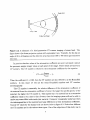
I
Figure
core.
2.1 A schematic
To appreciate
monochromatic
diagram of an x-ray beam system incident on a three-dimensional
the operation
of computer
tomography,
photon beam:_ of intensity I0 incident upon a homogeneous
_: The epithet monochromatic
source produces
and nomenclature
refers to a monoenergetic
a beam with a spectrum
object of width
photon beam; in reality an x-ray
of energy. In general, the attenuation
5
consider a
coefficient
d and density p. The intensity
is a function
of the beam after it penetrates
the object is/transmitted, it
of both d and p and it is related to I0 by the following relationship
/transmitted
k(p, £) is referred
to its density
monochromatic,
to as the attenuation-
-_ e-k(P'C)dIo
:
(1)
•
coefficient of the object and it is directly
p, and is a function of the incident energy E. When the incident
the dependence
of k on the incident energy is usually omitted
related
beam is
for brevity,
and one writes k(p).
When the object is inhomogeneous,
the distribution
the object.
then the intensity
after penetration
of density p(x, y, z) which the beam encountered
In this case the transmitted
/transmitted
intensity
--
e-
fL
depends on
along its path
through
is given by
(P(X'Y'z))dl_
L is the total path length and dl is the differential
O.
element along the path.
(2)
The integral
fL k(p(z, y, z))dl is referred to as the ray integral. In a conventional CT, the detector
signal is averaged over a short period of time and then digitized. Since the reference I0 is
known, by measuring
sets of/transmitted,
sets of values of the 1og(/traasmitted/I0)
provide
sets of the values of the ray integral fL k(p(x, y, z))dl along different paths L. A set of
such values of ray integrals is called a projection. Given a large number of projections,
one obtains a sufficient number of values of fL k(p(x, y, z))dl so that it becomes possible to
derive an approximate map of k(p(x, y, z)) throughout the two-dimensional
slice. Image
reconstruction
algorithms
are then used to assign different grey-level intensities
of values of k(p(x, y, z)) which lead to a two-dimensional
computer
to ranges
grey-scale image produced
on a
monitor.
Figure 2.2 shows a schematic
head. The detector-array
of a third generation
provides one projection
x-ray scanner imaging a patient's
,i.e., a set of values of 1og(Itransmitted//I0)
for every angle of the X-ray tube assembly.
also depends on the photon energy, and the polyenergetic
This problem is described in section 7.
6
beams produce imaging artifacts.
Detectors
X-Ray Tube
X-Ray Fan Seam
Figure
2.2 A schematic
of a third generation
figure shows a fan beam projection
CT scanner imaging a human
system with equiangular
head.
The
rays. Typically, the fan has an
angle of 30 to 45 degrees and the detector array has about 500 to 700 xenon gas ionization
detectors.
In practice absolute
values of the attenuation
coefficient are never calculated:
instead
the processor assigns integer values at each pixel of the image. These values are known as
CT numbers.
The CT number is related to the attenuation
coefficient by the equation
kasphalt
CT : K( _
1).
(3)
When the coefficient K = 1000, then the CT numbers are also referred to as the Hounsfield
numbers.
In this report
we will use the terms Hounsfield
numbers
and CT numbers
interchangeably.
The CT number
is essentially
the material from the attenuation
material,
the relative difference of the attenuation
coefficient of
coefficient of water; the larger the specific gravity of the
the higher the CT number is. This implies that if a material has an attenuation
coefficient which is very close to that of water, then the imaging system will not be able to
resolve any water-filled
the inhomogeneities
voids inside that material.
Computer
tomography
works best when
in the material have large differences in their attenuation
coefficients.
Typical CT values for the human body are shown below in figure 2.3. Notice how different
the CT numbers are for the various tissue types. One of the objectives of this study was to
7
determine
if sufficient differences in the CT numbers exist among the various components
of an asphalt/aggregate
-1000
I"
core to make asphalt tomography
'"/
I
Alle
-100
0
1
I
I
I
WAIEF_
possible.
100
1000
1"
' '/'
KIDNEYS I
I
[:':::':':'::'::':::'::::':':':':':':':':'::':':':':]
LIVER
BONE
[]
CONGEALED
BLOOD
Figure
2.3 Typical
CT values for the different components.of
the human
body.
After
together
with
Davison (1982).
Computer
sophisticated
tomography
systems
image reconstruction
use specialized
algorithms
dedicated
processors
to produce the final image.
The single most common beam systems in use for computer
systems,
which are now ubiquitous
applications
in medicine and in aerospace engineering.
the beam energies are about
In medical
denser materials.
ultrasound
applications
1500keV, because higher energies are required
to penetrate
(One such system was installed
type of tomography
waves instead of x-rays;
acoustic beams in a non-homogenous
as they scatter
emission tomography.
ation, whose discussion
used x-ray tomographic
tomography
its resolution
modalities
in 1989 at the Physics
is acoustic tomography
and sensitivity
material do not necessarily
and diffract at the interfaces
tomography
of an
industrial
sion of the Boeing Co.) Another
computer
are x-ray
the peak beam energies vary from 100keV to 130keV. One example
image from a medical scanner is shown in figure 2.4. In prototype
through
tomography
between
which uses
is much poorer because
travel in straight
different materials.
lines
Other related
include magnetic resonance imaging (MRI) and positron
However these are based on entirely
different
is beyond the scope of this introduction.
principles
MR] results had very poor resolution.
raphy is clearly ineffective for high resolution
ultra-sound scanners.
of oper-
In this study we only
imaging; however we did test the applicability
but our preliminary
Divi-
of MRI in core
Acoustic tomog-
core studies with the current generation
8
of
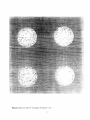
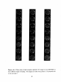
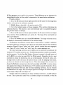
Figure
2.4 Four slices CT images of asphalt cores
9
Testing
an asphalt
furthermore
core with a medical
it does not leave any residual
diagnostic
medicine is a testament
CT does not alter its molecular
radioactivity.
The ubiquitous
structure;
use of CT in
to its relative safety.
Even though there have been a few applications
of computer
tomography
in imaging
soil and earth cores, CT had never before been applied to the study of asphalt or of asphalt
aggregate
cores. In our study we used a Phillips TX60 which is a third generation
CT scanner
and is located
x-ray
at Norris Hospital at USC. It utilizes a fan beam rotational
scanner similar to that sketched in figure 2.2.
In this report the imaging protocol of computer
described.
We have named our application
discuss certain applications
tomography
and its application
Asphalt Core Tomography
are
(ACT). We will also
unique to asphalt tomography.
Section 3 discusses many of the details necessary for perfoming the imaging protocol.
The CT scanner
3.1.
Section
cements.
settings
optimal
3.2 discusses
for asphalt
the determination
core tomography
of the CT numbers
Sections 3.3 and 3.4 explain the determination
the system detectability.
are described
The beam hardening(BH)
correction
asphalt
and of
is described in section 3.5;
for removing some of the image reconstruction
the polychromatic
nature of real x-ray tubes.
CT numbers,
of the SHRP
of the system resolution
this is a procedure
the aggregate
in section
artifacts
introduced
by
Section 3.6 discusses the determination
of
and section 3.7 discusses the determination
of the CT numbers
of asphalt mixes with fines.
Section 4 describes our morphological
studies.
Section 4.1 discusses the mass-fraction
calculations and section 4.2 discusses the large-scale deformation studies.
The conclusions and recommendations
are discussed in section 5.
Two extensive
mathematical
ASPlab,
appendices
are included.
Appendix
basis for the optical flow calculations.
the software developed and implemented
10
A describes
Appendix
in great detail the
B is a user's manual for
for routine core scanning analysis.
3. Development
col.
An imaging protocol
of the ACT Imaging
consists of a set of procedures
are used when imaging specific objects.
CT characteristics
and CT scanner
An imaging protocol
of the tissues or materials
under study.
Proto-
settings
that
also includes data on the
In medical imaging, there are
specific imaging protocols for "the various regions of the h-man body; for example, slightly
different operating
tissue.
parameters
are used when imaging brai:,
In this section we will describe all the operating
issue than when imaging neck
parameters
and the determination
CT data that were necessary in developing the Asphalt Core Tomography
The CT scanner settings optimal for asphalt core tomography
3.1.
Section
cements.
3.2 discusses
the determination
of the CT numbers
Sections 3.3 and 3.4 explain the determination
system detectability.
The beam hardening
correction
of the system resolution
and the
(BH) is described in section 3.5; this
polychromatic
nature
CT numbers,
are described in section
asphalt
for removing some of the image reconstruction
aggregate
protocol.
of the SHRP
is a procedure
of real x-ray tubes.
of
artifacts
introduced
by the
Section 3.6 discusses the determination
of the
and section 3.7 discusses the determination
asphalt mixes with fines.
11
of the CT numbers of
3.1 Determination
of the optimal scanner parameters.
CT was originally
developed
for human
studies;
operating
modified to yield optimal results for concrete/aggregate
We established
determined
a standard
imaging protocol
the optimal system parameters
cores of 15.24cm(6.0in)diameter
In particular
settings
have to be
cores.
for asphalt
core tomography,
by imaging two cylindrical
and of lO.16cm(4.0in)
we determined
parameters
and we
asphalt/aggregate
height.
the following optimal
parameters
for the x-ray
tube
:
X-ray peak energy --- 130kV
Beam intensity - 250mA
Scan time - 3msec
Slice thickness
These parameters
system parameters
produced
excellent
-- 3mm
grey-scale
images with good contrast.
such as the number of repetitions,
interslice spacing appear to be highly dependent
the number of projections,
on the specific application
contrast
3mm(O.12in)
However we
interslice spacing is necessary for achieving uniform
across the entire image, as well as the desired level of detectability.
Next we developed a specialized
from the CT computer
image processing format.
Phillips-made
for transferring
workstations.
by the CT computer,
Our unscrambling
CT scanners;
for transferring
algorithm
to SUN and Macintosh
CT image data are scrambled
vendors
and the
and the resolu-
tion desired for 3-D studies and they do not depend on the single slice data.
found that a maximum
Other
the CT image file data
For proprietary
and they are not stored in a standard
algorithm
is specific to images generated
Several software packages have been announced
data from CT computers
in standard
TIFF files). This is discussed further in the appendix on ASPlab.
.12
reasons, the
image format
by
by various
(PICT
or
3.2 Determination
of Asphalt CT Numbers.
To obtain quantitative
essary to have accurate
information
from an asphalt/aggregate
core image, it is nec-
CT numbers for the different material components
core. This is necessary to properly identify the different components
aggregates,
asphalt-aggregate
forward as it appears;
introduced
uncorrected
by constructing
algorithms
the CT values of asphalt we followed a standard
At first, a plexiglass phantomt
had nine 2.54cm(1.Oin)
tubes of different asphalts
performed satisfactorily,
another phantom
was designed to reduce the beam hardening
The new phantom was manufactured
was constructed.
top lid had nine 2.54cm(1.0in)
diameter
and were lined with rubber
deviation
The
height
around their
the test-tubes
and therefore
with
the new
diameter,
0.635cm(0.25in)
high with two circular plates as lids. The
for sealing.
for the
In the same lid we drilled a
hole for bleeding out the residual air remaining
after the phantom
t A phantom is a lucite cylindrical box with known CT characteristics
used to calibrate the CT scanner.
13
CT
effect.
holes; these holes were the receptacles
O-rings
for these
were reliable asphalt
which surrounded
by using 15.24cm(6.0in)
lucite pipe, and it was 10.16cm(4.0in)
0.635cm(0.25in)
procedure
effects accounted
water; water is known to have relatively small x-ray attenuation
test-tubes
calibration
except that the CT values obtained
to ensure that the values obtained
values. Therefore, we constructed
thickness
for human
cylindrical bore holes and it was used to hold test-
mean values. Even though it was evident that beam hardening
phantom
for compensating
and of lO.16m(4.0in)
for the different SHRP asphalts showed a relatively large standard
it was important
CT sys-
during CT scans.
This plexiglass phantom
deviations,
which are
as regions of higher asphalt/fine-
was a solid lucite cylinder 15.24cm(6.0in)diameter
The phantom
artifacts
they are have been developed specifically
a water phantom.
voids,
This is not a straight-
of the x-ray beams in commercial
mix density Medical CT scanners have standard
To determine
phantom
nature
these artifacts could be interpreted
for these effect, but unfortunately
studies.
(i.e., asphalt,
CT images have beam hardening
due to the polychromatic
tems. If uncorrected,
aggregate
mixes) during image reconstruction.
composing the
had
and is routinely
been filled with water.
In normal operation,
test-tubes
asphalt cements were poured
in the pyrex test-tubes
were placed in the holes; then the phantom
metrical configuration
was identical
the inner space between adjacent
Figure 3.2.1 shows a photograph
Using this phantom
was filled with water.
to that of the plexiglass phantom,
test-tubes
This geo-
except that now
was filled with water instead of solid lucite.
of the lucite phantom
we obtained
and the
with several asphalt test-tubes.
the following values for the attenuation
coefficients
of six SHRP asphalts.
Table
Asphalt
3.2.1
Hounsfield#
AAM-1
AAG-1
AAB-1
AAA-1
AAD-1
AAK-1
These numbers
were performed
geometric
-62.00
-25.80
-14.40
-4.40
22.20
34.30
are averages of eighteen different trials for each asphalt.
These trials
using two diffei'ent fillings from each of the SHRP asphalts, three different
arrangements
for each samples within the lucite rack, and using three different
elevations with respect to the top of the rack. The CT number in each trial was determined
using the Region of Interest
approximately
(ROI) operation
lOOmrn2(O.16in2),
of the CT computer.
and the CT number variations
The ROI we used was
between trials were less
than 5%, except for the AAG-1 asphalt where it was less than 10%. 1:
These attenuation
SHRP asphalts.
the asphalts
correlated
values were then compared
The most interesting
well with higher Hounsfield numbers.
type mouse.
average CT number.
Appendix
is performed
The computer
of the
results were derived when the metal content
was plotted with the Hounsfield number; as expected,
:[: The ROI operation
roller-point
with the chemical composition
of
higher metallic content
These results are presented in figure 3.2.2.
by selecting of any arbitrary
closed contour
by a
displays the enclosed area in mm 2 and then the
The same operation
exists in the ASPLab
B.
14
software
described
in
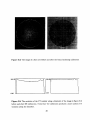
Figure
3.2.1
A photograph
of the lucite phantom.
15
Energy level = t20keV
2000
,
I
I
I'
,
I
'
-
'
AAK-_
-
4ooo
AAG AAB-_'-4
I _.......E_..EYE;_
-?AM-,.
_Y
>
-
-0.06 -0.04 -0.02
0
0,02
0.04
A meosure of the ottenuotion coefficient
Energy level = t20 keV
t60 1
I
I
I
Ill
_
I AIAD
,oo ••
20
AAM-t
_ J
II
t II
I
'
l
J
//
i
I
-0.06 -0.04 -0.02
I
r
J
0
I ,i
0.02
-I
J /
0.04
A meosure Of the ottenuotion coefficient
Figure
3.2.2
Attenuation
data as a function of the metal content of different asphalts.
16
3.3 Determination
It is customary
of the System Resolution
in CT investigations
a nominal system performance
function
parameter
(PSF). This parameter
to determine
the system resolution
by calculating
referred to in signal processing as the point spread
is a measure of the smallest geometric features which can
be identified by the CT scanner.
To appreciate
this parameter,
consider the CT monitor
display which normally
con-
sists of a square array of 512 × 512 pixels. Since the imaging test area is approximately
129cm2(20in 2) , then approximately
mapped
in one pixel.
every area of lmm2(O.O16in 2) of the test object is
One could conclude that
the resolution
is about
approximately
lmm(O.O4in).
To obtain a reliable estimate
of the system resolution,
wire was imaged in an air phantom.
the test-tube
and the phantom.
there are 2pixels/mm,
a 0.4mm(O.O15in)
Figure 3.3.1 shows an image of a section of the wire,
If the system had had perfect resolution,
and since the
then the wire should occupy one pixel in the display.
shows the actual results.
The figure shows the distribution
between 0 and 320 as a function
numbers.
platinum
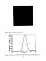
Figure 3.3.2
of CT numbers
of the distance perpendicular
normalized
to the wire axis, in pixel
This plot depicts the PSF. The centerline of the wire is at approximately
Under ideal conditions,
delta function.
at an elevation
one would expect to see a single line at that location, similar to a
Instead,
nominal CT resolution
it is clear that the image "spills" over into adjacent
is determined
exactly
320, and the half-width
of 2.3mm(O.O9in).
system resolution;
by measuring
half the maximum
the width in pixels of the distribution
CT number.
Note that
the system detectability
resolution
In this case the maximum
images of small dense particle may "bleed" into adjacent
obtained
pixels making
is further discussed in the next section.
to note that the PSF is dependent
The resolution
is
may be higher than the nominal
on the Hounsfield number.
has density much higher and therefore lower attenuation
asphalt.
pixels. The
at 160 is 4.63 pixels; this implies a nominal system resolution
them visible. This phenomenon
It is important
12.5pixels.
using the platinum
of the system.
17
Platim,m
than the density of aggregate
or
wire is clearly an upper limit of the
Figure
3.3.1 The image of a platinum
_n 260
N
l.
wire.
I
I
240
220-
_- 2O0.0
E t80z
t60-
----
_J t40•_
t?-0-
I
I
I
I
"6 t00 -
_
I
o
I
I
E
I
80-
z
I
606
Figure
5
_o
,I
Pixels
i
i I
45
20
25
3.2.2 The point spread function (PSF) derived from the image in figure 3.3.1.
18
3.4. System Detectability
As discussed in the description
of the previous test, the system detectability
much larger than the system resolution.
protocol,
we conducted
est particle
To determine
the detectability
a special test with two objectives.
size that is detectable
may be
of the imaging
One, to determine
with the ACT, and two, to determine
of the small-
of the smallest
identifiable distance between two adjacent particles.
A. Determination
of smallest
Several 2.54cm(1.0in)
vation,
approximately
detectable
test-tubes
half-way
particle
size.
were filled with AAG asphalt
up to the top.
We then placed a 3mm(O.12in)
marker particle on the initially free asphalt surface in each tube.
as the test surface; the marker particle
up to a specific elemetallic
We refer to this surface
allowed us to locate the image of the test surface
quickly with the CT computer when scanning the entire tube. We then located glass beads
and sand grains of different sizes on the test surface, and we drew an approximate
particle sizes and sand grains sizes for the test surface in each tube.
map of
An example of this
map is shown in figure 3.4.1. Then the tubes were filled with asphalt to the top, so that
the test surface could now only be identified through
The test-tubes
The CT scanner's
CT images.
were then imaged both in the plexiglass
gantry was moved incrementally
was located in the CT monitor; subsequent
By visual inspection
until the surface with the marker beads
slice images were obtained
of the CT display monitor,
and sand grains down to sizes of 0.46mm(O.O18in)
than the 0.37mrn(O.O14in)
and in the water phantoms.
every lmm(O.O4in).
it was possible to detect glass beads
on our test surface.
Particles
particles smaller were not detected.
We did not find any significant differences in the lower limits of detectability
the glass and the sand particles.
that the protocol
the detection
smaller
Since metallic materials have low attenuation,
between
we expect
should detect metal grains down to the O.lmm(O.OO4in) size ; however,
of metallic particles of this size was not attempted.
The detectability
was also checked using the cross-hair
able on the CT console for obtaining
test surface and we positioned
cursor and the joystick avail-
specific data from the display.
the cross-hair
19
We displayed
at one side of the perimeter
the
of one of the
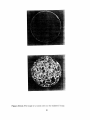
WATER BATH PHANTOM (WBP)
6
5
Figure 3.4.1 Map of the particles which were placed inside an AAG asphalt
tube to determine the detectability of the system.
2O
filled test-
smallest visible beads and noted the co-ordinates
cursor to the diametrically
ordinates
again.
We thus calculated
size to 0.60mm(O.O23in)
observations
B. The
opposite
diameter.
side of the bead perimeter,
that can be identified.
close together
and we noted the co-
Since the cursor is at least 0.4mm(O.O16in)
suggest that the system d_tectability
determination
of the smallest
thick, these
is 0.5mm(O.O2in).
detectable
separation
distance.
of the system is the smallest separation
distance
Images of small particles bleed to adjacent pixels and small particles
may appear as a single larger particle.
It was not possible to locate submillimeter
Therefore,
we designed another
size particles at fixed distances on the test
test by carefully filling a test-tube
AAG after placing two 1.8mm(O.OTOin) bore glass capillary tubes.
coplanar,
We then moved the
the size of a particle known to be 0.46mm(O.O18in)
Another measure of the detectability
surface.
from the display.
with asphalt
The two tubes were
but not parallel and they converged to a common vertex. The sample was then
scanned
and images were obtained,
until it was no longer possible to identify the two
separate
tubes (i.e., until the tubes appeared
fused together).
Based on our results, we conclude that the smallest separation
with the Phillips scanner is of the order of one-tube
Note that the detectability
than the limiting separation
This limitation
core because
detectable
(i.e,l.8mm(O.OTOin)).
of the system (in terms of particle
size) is much smaller
distance, since the images of small particles smear on adjacent
pixels. A single small particle surrounded
of two small particles
diameter
distance
very close together
has practically
by asphalt is easily identable; however the images
appear
as the image of a single large particle.
no effect in the mass-fraction
the combined image has aproximately
calculations
for the entire
the same image area as that of the
sum of the areas of the two particles.
This one-particle
size limit on the detectability
not be possible to accurately
smaller than 1.00mm(O.O4Oin).
obtain the particle
Particles
of small particles implies that it may
distribution
function
for particle
larger than this size have distinct
CT images even when adjacent to each other.
21
sizes
shapes in the
Determination
Beam hardening
polychromatic
of'
Hardening
eam
Correction.
arises from the polychromatic nature of x-ray beams. A characteristic
x-ray spectrum
is shown in figure 3.5.1.
counts incident on an x-ray detector
The figure shows the number of
as a function of the energy of an x-ray tube._
• - ..:_.-..
.-22'.
u
2
,0
&
4,
_.
_
£r_rgy
Figure
3.5.1
' .
'
in
An example of an experimentally
K_V
measure
x-, _:sytube spectrum.
From
Epps and Weiss (1976).
To appreciate
how this x-ray spectrum
beam with Nin photons
penetrate
entering through an object and suppose that
through this object.
numbers of photons
According to equation
to energy deposition
Ytransmitte
d
photons
(2), the entering and the transmitted
are related by the equation
Ntransmitte
The ionization
affects the results, consider a monochromatic
d "- e- f L k[p(x'Y'z)ldl
(4)
Nin.
detectors employed in the Phillips CT system used in this study respond
per unit mass and do not actually
the effect is qualitatively
the same as in systems
1979).
22
count individual photons; however
responding
to energy deposition
(Kak,
If the beam is polychromatic,
then this equations should be replaced by the following
gtransmitte
d -- /
Sin(E)e-
fL k[p(x'Y'Z)'£]dldE.
(5)
Sin(E) is the incident photon number density in the range between E and E -b dE, i.e., it
is a probability
density
function.
Notice (Kak, 1979), that in equation
tion coefficient k[p(x, y, z), E] is also a function
range used in CT, the attenuation
Therefore
in a polychromatic
or scattered,
spectrum.
energy E. In the energy
coefficient generally decreases with the incident energy.
beam, the lower energy photons are preferentially
and the peak of the exit spectrum
absorbed
maybe higher than the peak of the incident
This is the beam hardening effect we referred to earlier.
As a polychromatic
etrates
of the incident
(5) the attenua-
x-ray beam with a continuous
a plane of a uniform object, the variation
distribution
of the attenuation
of energy levels pencoefficient with the
beam energy level produces a variation of CT numbers through the plane. Lower lowerthan-actual
CT values near the center of the object are then obtained and consequently the
image of the slice appears darker near the center than near the edges. This effect is shown
in figure 3.5.2. Without
correction,
this artifact may lead to a serious misinterpretation
the image. For example, darker areas at the center may be interpreted
asphalt
than surrounding
as containing
of
more
areas.
To remove this artifact, a beam hardening correction fui, :tion was applied to transform
the CT image.
function
This was done through
of a non-linear
which was then applied to filter the reconstructed
function was determined
to as the beam-hardening
The correction
prepared
the calculation
by measuring a standard
This transformation
correction image, and it is often referred
kernel.
image was obtained
a 7.62cm(3.0in)
image.
tranformation
by imaging a specially constructed
diameter and 10.16cm(4.0in)
with finely crushed granite ds < 0.5mm(O.O2in)
We
high core with AAG asphalt mixed
to a very uniform consistency.
imaged the core at three different energy levels and at three different
the core is uniform by construction,
core.
under ideal conditions
Then we
elevations.
Since
the image of the core should
have had uniform gray intensity; yet the center area of the image was slightly darker than
the edge area. This effect was obvious in all our uncorrected
cores. It can be seen in the images in figure 3.5.5a.
23
images of asphalt/aggregate
.278
Monoc]_zon'_cCese
.265
,
,
I
I
,
- 1.00
,
,
,
,
,
,
0
1.00
Distance from the Center
Figure
tom
3.5.2
using
the beam
cient
(a) Reconstructed
a polychromatic
hardening
through
monochromatic
effect.
a a diametral
x-ray
beams.
image fxom projection
source.
The
(b) A sketch
whitening
data
seen near
of the variation
line of the water
After Kak(1979).
24
phantom,
of a surface
the edges
of the linear
both
of a water
with
phan-
of phantom
attenuation
polycromatic
is
coeffiand with
The variation of the attenuation
coefficient (in CT number units) as a function of the
relative radial distance from the center normalized
3.5.3a and 3.5.3d. The ordinate
with the core radius is shown in figures
is the CT number CT(r, z, g) averaged over all azimuthal
angles ¢. In our cylindrical co-ordinate
system r is the radial location measured
center, z is the elevation, and ¢ is the azimuthal
from the
angle. The abscissa is normalized
so that
the number 100 indicates the core edge and the number 0 the sample center. Figure 3.5.3a
shows the variation of the CT number at the three different elevations z for three different
beam intensities
IOOkEV, 120kEV
a different energy
Without
and 130kEV.
Each group of three curves represents
level, while each curve in the group represents
the beam hardening
effect, these curves would collapse into one straight
Clearly there is little difference in the distribution
of CT numbers
vations; however there is some difference in the distribution
beams with different
a different elevation.
intensities.
line.
at different ele-
among images derived using
This is also seen in figure 3.5.3b; here the same image
plane was scanned three different times without
removing the core from the CT gantry.
This is quite a helpful result because it allows the use a single beam hardening
correction
function for all slice data (i.e. for the entire core), for any given beam intensity.
We determined
the two-dimensional
core analysis using standard
nonlinear
transformation
image processing methods.
function
f(p; ¢) for
The objective was to find a kernel
which, when applied on every pixel x, y of a fine-aggregate
core image, it would produce
uniform gray intensity over the entire image area. Given figure 3.5.3,
this kernel does not
depend on the the elevation z inside the core, but only on the energy level.
In order to determine
aggregate
the effectiveness of the kernel that we havedeveloped,
core was constructed
with the same overall density as the fine-aggregate
which was used for the kernel determination.
energy level as the fine-aggregate
performing
correction.
core. The results of these scans are shown in figure 3.5.4.
package (ASPlab)
described
core before performing
the
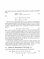
Figure 3.5.4a shows images of the same slice before and after
the beam hardening
We have incorporated
core
Then we imaged the coarse core at the same
Figure 3.5.4a shows the image of a section of the fine aggregate
beam hardening
a coarse-
correction.
this operation
in appendix
function to perform this correction.
in our asphalt
core image processing
B. In ASPlab there
software
is a specific menu driven
The software uses the standard
calibration
image with
AAG asphalt shown in figure 3.5.4a. There is very little difference in the beam hardening
25
3000
2000
.....
_.. ....
1000
i
-100
Figure
elevations
3.5.3a
0
100
Plot of the function CT(r, z, E) = fo f(r, ¢, E)d¢ for three different axial
and for three different energy levels.
3000
2oo0
_J
_T._.T._._.T_._.___L__.T.TT.T___.._._.y._L_._._7-.7..._;`:_::.__.
1000
0
-100
,
i[
0
100
Figure 3.5.3b Plot of the function CT(r, z, E) = fo f(r, ¢, C)d¢ for three different ener_,
levels at the same axial elevation.
26
correction
function
same correction
between
between
the different SHRP asphalts,
can be used for all asphalt cores with asphalt mass fractions in the range
5.5% to 6.5%. Further,
the procedure
any core with diameter less than 25.4cm(10in)
For determining
significantly
and we are confident that the
the beam-hardening
described
in appendix
B can be used for
and it does not depend on the core height.
correction
for coarse cores with mass fractions
different than 6.0% + 0.5, we propose the following procedure
the beam hardening
correction.
A) If the mass fraction of the sample is known by some other method
a fine-aggregate
for performing
core of the same mass fraction should be constructed
image should be obtained.
or by design, then
and a calibration
Then ASPlab can be used to determine the kernel for correcting
the images of the original core and for verifying its mass fraction.
B) If the mass fraction
preliminary
in not known,
mass-fraction
with that preliminary
a calibration
then ASPlab
value, without
can be used first to determine
any corrections.
Then a fine-aggregate
mass fraction value can be constructed
a
core
and then be used to obtain
image.
C) If it is not possible to construct a fine-agregate core, the ASPlab operation SELFCALIBRATE can be used. This operation will produce qualitatively correct images, but
care should be used in interpreting
3.6 Determination
the mass fraction results obtained
of the Aggregate
As discussed earlier, determination
in this manner.
CT Numbers
of quantitative
mass-fraction
data from a set of
ACT slice data requires knowledge of the CT numbers for all the different components
the core, so that these components
of
can be properly identified during image reconstruction.
In this section we present results on the SHRP aggregate
CT numbers.
In our preliminary work, we determined aggregate CT numbers by locating the crosshair cursor of the CT display directly on aggregates images inside a core and then reading
off the CT number.
exist between
That
data was used for demonstrating
the CT numbers
of asphalt
that
significant
differences
and of aggregates to thus allow unambiguous
27
Figure
3.5.4a
Two cross-sectional
after the beam hardening
241.00 _
Figure
3.5.4a.
3.5.4b
images of the asphalt/fine-aggregate
core before and
correction.
250.00_"_.,.,,
The variation in the CT number along a diameter
28
of the images in Figure
identification
of these components.
the CT numbers
However, when we measured the standard
in large aggregates
we noted that the standard
deviation
inside the core using the ROI operation
of
of ASPlab,
deviation
was relatively high, possibly because of absorbtion
deviation
and to obtain more representative
of the asphalt.
To reduce the standard
imaged test-tubes
filled with crushed aggregate
standard
probably
deviation
grains.
CT numbers, we
The data showed a substantial
because of the air voids entrained
in the fine-grains
column
during packing.
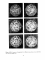
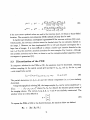
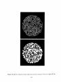
Finally we performed
aggregate
a systematic
series of tests by placing the largest size SHRP
particles that would fit inside water-filled
the tomograms
used to obtain
aggregate
petri dishes. Figure 3.6.1 shows six of
CT numbers.
The standard
deviation
obtained
was smaller than before and it appears possible -in some cases- to identify the aggregate
type by its CT number.
Table 3.6.1 lists the CT numbers of seven SHRP aggregates using three different beam
intensities.
The mean values shown in the second column are mean CT values obtained
by averaging
column.
CT data over an area containing
The third column shows the standard
the standard
deviation
aggregate
of the CT Nllmbers
in section 3.4, the smallest particle
is 0.47mm(O.O18in).
particles
Therefore
particle concentration,
measured in
of Asphalt
Mixes with
which can be detected
it is not possible to identify individually
inside asphalt/aggregate
the density of the material,
deviation
the same size in a pure asphalt core.
3.7 Determination
Fines
protocol
deviation over the same region. Even though
is not large, it is greater than the standard
a region of approximately
As discussed
the number of pixels shown in the fourth
smaller
mixes. However, the CT number depends on
and it is therefore plausible to attempt
i.e., the mass-fraction
with this
of a fine -aggregate
to determine
the local
mix from the ACT data.
Assume that the CT number of a pixel in the image is written as CTpixel and assume
29
Table
Aggregate
Table
3.6.1
CT Numbers
keV
Mean
Value
Standard
Deviation
RA
100
120
130
2475.0
2184.0
2015.0
48.25
43.25
41.75
234
329
284
RB
100
120
130
3157.5
2738.0
2530.0
48.1
19.9
19.0
622
606
571
RC
100
120
130
3130.0
2918.0
2699.0
37.0
61.0
57.0
286
322
302
RG
100
120
130
2900.0
2530.0
2350.0
95.0
92.0
73.0
428
550
348
RJ*
100
120
130
2049.7
1816.0
1704.3
153.0
105.0
100.3
559
484
485
RL*
100
120
130
2343.0
2072.7
1930.7
134.0
110.2
110.5
235
259
277
3.6.1 A table of CT values for the different SHRP aggregates.
3O
No. of
Pixels
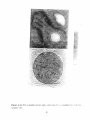
Figure
3.6.1
Six images
of aggl'egate
particles
31
in a water bath.
that the CT numbers of the asphalt and of the aggregate
respectively.
Then the following relationship
CTpixel
-- _CTasphalt
where c_is the local mass-fraction
occupied
by the asphalt
aggregate.
are
CTasphal
t
and CTaggregate
holds true :
(1 - _)CTaggregate,
Jr
of the asphalt,
(6)
i.e., c_ is the fraction of the pixel volume
and (1 - c_) is the fraction of the pixel volume occupied
If a relationship
between CTpixel and c_ is established,
by the
then it should be possible
to identify the mass fraction c_anywhere inside the core.
To determine
phalt mass-fraction
this relationship,
twelve cores were constructed
with the following as-
ratios 0.04, 0.045, 0.05, 0.055, 0.06, 0.1, 0.2, 0.3, 0.4, 0.5, 0.6, & 0.7. Even
though most pavements
identify a relationship.
are in the 0.03 to 0.1 range, the entire series of data is needed to
Each core was prepared with asphalt AAG and with RC limestone
aggregate crushed as fine as possible.
These cores were then imaged to determine
of the mix density on the correction
image.
The CT number for each fraction was determined
correction,
simply by averaging
operation.
The experiments
prepared
the CT number
were performed
without
the effect
using a beam hardening
over the sample area, using the ROI
in a double-blind
fashion.
The cores were
by the LA County Materials Lab and they were only known to us by code. The
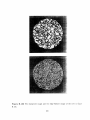
images are shown in figure 3.7.1.
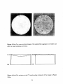
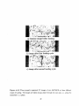
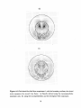
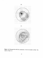
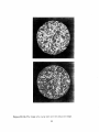
Figure
3.7.1 is a print with 8 tomograms
which are presented
from the scans used to derive the data
in figure 3.7.2. The curved surface underneath
each sample is the CT
gantry bed; this artifact is routinely removed from the images using the ASPlab software,
when the beam-hardening
correction is performed. However, since the beam hardening
correction kernel for every mass fraction is determined by preparing fine-aggregate cores
of that fraction, this correction was not performed here; it made little sense to correct
a set of data with the same data. The beam hardening correction is only neccessary for
obtaining
quantitatively
correct coarse-core
Figure 3.7.2 shows the variation
images.
of the mix CT number with the % asphalt
in the mix, for three different energy levels. As expected,
content
the CT numbers decrease as the
mix density decreases, i.e., as the % asphalt content increases.
Notice that no data is shown for mass-fractions less than 10%. The 4%, 4.5%, 5%, 5.5%
and 6% cores did not produce any significant differences in the CT numbers.
32
This result
Figure
3.7.1
Tomograms
of eight different
fine-aggregate/asphalt
cores
0
0
0
0
0I
0
U3
0
U3
0
0
(AerObe) _aqwnu 13
0
I
'
_
_
0
..
0
1_
_
_ ©
.._
..-
0
O
O_
O"D
_
0
0
0
I
0
0
0
0
0
_
0
0
0
0
0
0
by-weight
3.7'.2 The variation
I
0
0
0
I
0
0
,n
'0
0
(Aa_100|} j_qcunu 13
(Aa)lO_|) JaquJnu13
Figure
I
0
0
,_
of th(, CT number with the asphalt
units for three different energy levels.
34
content in percentage
implies that -in the range of mix-density
cores- the CT number
values most often used in pavement-grade
depends only weakly on the density.
Therefore
the same beam-
hardening correction kernel can be used for cores with different densities,
core has an asphalt fraction less than 10_.
We did not perform experiments
quantitative
behaviour.
with different aggregates,
The fines are a small portion
asphalt
as long as the
but we expect the same
of the total aggregate
in the mix,
and small errors is determining the mass-fraction in the fines will not affect significantly
the estimate of the mass-fraction for the entire core.
The CT mix-density
local mix density
asphalt
the aggregate
suggest
that it is only possible to identify
the
at any given microscopic region of the core to within 20% of the true
mass fraction.
only a fraction
data obtained
However, since in most real cores the fines portion
of the overall aggregate
fraction,
the overall error in the determination
mass fraction in the large aggregate/fine
and scatter
type in the mix may introduce
calculation.
a result in the range 4.75_
in the CT values because of the particular
another
aggregate
0.25% absolute error in the final mass-fraction
35
of
core is not expected to exceed 5_.
For example, when imaging a 5% core, ACT should produce
to 5.25%. Uncertainty
of the core is
4. Morphological
Calculations
The most interesting
Studies and Mass Fraction
application
of asphalt
mass fractions and the visualization
core tomography
is the determination
of large internal deformations.
of
We will describe these
results in the following sections.
4.1 The determination
cores.
of the mass fraction of asphalt/aggregate
With the software tools developed and the CT component
possible to estimate
procedure
components
frequency
core.
the mass-fraction
involves establishing
of the different components
certain threshold
in the mix and then calculating
of occurence
Using standard
was determined.
of the different
methods
number of pixels with CT numbers
the mass-fraction
from histogram
of CT numbers
ranges for asphalt
in these ranges was determined.
36
of individual
of the
in each set of slice data for a given
distribution
threshold
it is now
in a mixed core. This
ranges for the CT numbers
CT numbers
the frequency
Then, by establishing
data obtained,
over a core-slice
and aggregate,
the
When divided by the
total number of pixels in the slice, one obtains directly the area fraction of the particular
component
with CT number in the range chosen, This area fraction is clearly an average
of the actual volume fraction over the thickness of the individual slice. Integrating
area fractions over the entire core determines the volume fraction.
Recall that slice data are obtained
there are several "empty"
image reconstruction
at a 3mm(O.12in)
algorithms do exist for interpolating
Therefore
the data in these "empty" region
it is a trivial matter to integrate
and to obtain
i.e., the number of pixels of asphalt in the entire core is divided by the
total number of pixels in the core. Multiplying
of the asphalt in the mix produces one estimate
we have incorporated
fraction calculations.
spacing.
regions in the core for which no CT data exist; however standard
between adjacent slices. After interpolation,
the volume fraction,
inter-slice
these
this volume fraction by the known density
of the asphalt mass fraction in the core.
in ASPlab a special operation
Our algorithm
is more complicated
(script)
for performing
than what described
mass-
above; the
ASPlab script also accounts for the asphalt present in the asphalt fine--aggregate
mix.
Data for two different cores are shown in table 4.1. The mixed core contains all grades
of aggregate
particles,
2mm(O.O78in).
while the coarse core only contained
Both cores were specifically constructed
the density for which the beam hardening
The experiments
correction
were again conducted in double-blind
aggregate particles larger than
with a 6% density because this was
function (section 3.5) was developed.
fashion. The cores were only known
to us by code.
Table
Determination
of mass
fractions
4.1
for asphalt
aggregate
cores
Coarse
Mixed
Aggregate
core
Aggregate
core
TRUE ASPHALT MASS
ESTIMATED ASPHALT MASS
70.5g
88.5g
72g
71.9g
TRUE AGGREGATE MASS
ESTIMATED AGGREGATE MASS
TRUE MASS FRACTION
EXTIMATED MASS FRACTION
1105g
l102g
6%
7.2%
1128
1133
6%
5.97%
37
It is clear that ACT adequately
that it also overestimates
intuitively;
deadlines
estimates
the mass fraction of the mixed core, but
the fraction in the coarse core. This is not what one would expect
ACT should be less accurate when estimating
imposed on the project
experiments,
did not permit
the mixed core. Since the SHRP
verification
of these results with serial
we are hesitant to draw definitive conclusions as to the expected error of the
mass fraction calculation.
Clearly more experiments
are necessary,
necessary
to validate
these results.
4.2 Visualizations
There
of large scale deformation
are two major
in two dimensions.
sets of image data which can be obtained
studies beyond the usual CT slice data. One is the visualization
induced by loading and the determination
of aggregate-particle
in morphological
of large-scale
migration
deformations
patterns;
as we
will report, ACT can even be used to measure the displacement field. The other is the
three-dimensional
visualization of the core and the calculation of image data along any
arbitrary
plane surface through the core. The latter is discussed in section 4.3. t
Numerous
core images are presented
throughout
this report.
be made that these images do not provide any morphological
the information
dye-chemistry
methods
which can already
technique
for obtaining
introduced
mass-fraction
be obtained
An argument
information
could
additional
by other imaging methods
to
such as the
by Lee et al (1983).:_ Also, there are easier standard
data.
However, all other existing
methods
which
t In this part of our work we would like to acknowledge Professor Carl Monismith
of the
University of California at Berkeley of SHRP-A003
these tests.
:_ Note that
the dye-chemistry
technique
for providing us with the cores used in
does not provide any distribution
density data for mixes with fines. Also ACT has five times higher resolution
chemistry
imaging method.
38
data
or
than the dye
provide morphological
data similar to that of ACT are destructive;
data the core has to be physically destroyed.
phological data without
that is to measure the
Only with ACT is it possible to obtain mor-
altering the core structure.
The non-destructive
nature
of ACT
allows for the successive imaging of cores before and after loading and the visualization
the associated
deformations
To demonstrate
scale deformations,
of
and particle displacements.
and to evaluate the application
we obtained
four lO.16cm(4.0in)
of ACT in the visualization
cores from SHRP-A003;
of large
these cores
were known to us as only by code. The following testing protocol was used :
1) A metal marker particle (referred to in CT as a Bigley spot) was placed on the perimeter
of the base of one of the cores to provide a reference marker for image registration.
2) Baseline image data was obtained
for each core in the condition received.
3) The cores were then loaded following standard
diametrical deformation.
ASTM procedures
up to 2.54mm(O.lO)in
4) Using the marker particle as a guide, the cores were placed at approximately
the same
place on the CT gantry and a new set of image data was obtained.
5) The cores were then loaded again as in step 3.
6) The cores were imaged again as in step 4.
A typical loading cycle for core is shown in figure 4.1; this particular
test was the load-
ing test for core B4 BOWlFD. The ordinate is the loading force applied in pounds and the
abscissa is the diametrical deformation in inches. None of the four cores exhibited plastic
failure during the first loading cycle. In the second loading cycle, continuous
of a core without
and it resulted
deformation
any change in the loading force was considered to indicate plastic failure
in the termination
of the loading test. One core (5BlWOFD)
the second loading cycle. Two cores had visible signs of permanent
failed during
deformation
after each
cycle but did not fail.
Figure
4.2.2 shows a sequence
5B1W0 FD core at three different
images were obtained
of tomograms
loading stages.
of six different
cross-sections
A total of forty-two
of the
cross-sectional
for every core at baseline and after each loading cycle. Figure 4.2.2a
is the baseline sequence of images for the unloaded
images of approximately
core.
Figure 4.2.2b is a sequence of
the same core surface as figure 4.2.2a, after the first loading cycle.
Figure 4.2.2c is a sequence of images after the core has failed.
this figure The crack width varies from lmm
to 3mm(O.O4in)
39
A large crack is seen in
to 9mm(O.12in).
The crack
Doto from "B4 BOW1 FD"
o._z
'
I
'
I
'
I
'
I
'
- D run t
(13
W
0,t0-
0 run 2-0
- • run 2-o
0_8
- ¢ run 2-b
:z
(9
z
l-I
D 0 •
1
Z
uJ 0.06W
r_
--
0.04J
13.
_°°
o 002-,
0,00
D
-_. I
0
4.2.1
I
0
1
_
--
-
(_
l
I
200
I
300
LOAD
Figure
•
$
I
t00
D
"-
_
0
•
•
.
A typical loading curve for the A003 cores.
4O
I
I
400
,
500
Figure
4.2.2a
A sequence of tomograms
of six different cross-sections
before loading.
41
of core 5B1WOFD
Figure 4.2.2b A sequence of tomograms
after the first loading cycle.
of six different cross-sections
42
of core 5B1WOFD
Figure 4.2.2c A sequence of tomograms of six different cross-sections of core 5BI\¥0FD
after the second loading cycle. A large crack is visible in the upper right and left images.
43
propagation
path is quite interesting;
the crack is seen to diffract around large aggregate
particles. Similar results were obtained with the other core which failed; there it is possibly
to see crack bifurcation, i.e., where a crack starts branching out as the load increases.
These results are quite useful in validating
for studying
the mechanical
digitizing the aggregate
finite--element
aspects of asphalt-aggregate
particle
models under development
during loading.
By
it is possible to assign an initial pattern
for
boundaries,
interaction
the finite-element
grids. By comparing the model results after loading
laboratory results, the validity of these models can be evaluated.
A substantial
image-flow
advance
analysis protocol.
motion of structures
this motion.
uniqueness
studying
of an
Optical flow analysis refers to the process of studying
in sequences of images to determine
of the solution.
However, considerable
the velocity
the
field that produces
progress has recently been achieved in
the motion of the heart in CT chest-images
relatively
is the development
This is a notoriously difficult problem in image processing because of the non-
We conjectured
straints
which was achieved in this study
with the ACT
that ACT is an ideal application
small and the number
of structures
(Song and Leahy, 1991).
for this method.
(aggregate
particles)
The motions
imposes certain
on the solution field, making the velocity field easier to compute.
are
con-
An example of
the results is shown in figure 4.2.3. The vectors overlaid on the images show the magnitude
and the direction of the velocity of each pixel in the image. An extensive discussion of the
image-flow
analysis is given in appendix
One useful method
two-dimensional
for visualizing
streamfunction
A.
flow patterns
The
_(x, y) is defined through the equations
0_
Oy
0_
-- u and
where u and v are the velocity components
of constant
is by using the streamfunction.
_ values are streamlines;
Ox
= -v,
(7)
in the x and y directions along any plane. Lines
in steady flow they are also the streaklines.
flows these lines are generated by injecting dye at a specific flow location.
formed by the different streamlines helps visualize the flow.
Figure 4.2.4 shows the streamline
pattern
for the deformation
The pattern
field calculated
4.2.3. The flow pattern in this figure is more useful for visualizing the migration
of particles in the flow field.
44
In fluid
in figure
patterns
Figure
4.2.3
Demonstration
of image flow calculations.
Two registered
color images of
the core 5B1WOFD at baseline and after the second loading cycle.
4.3 Three--dlmensional
morphological
In this section we will present
studies.
data showing deformation
patterns
along arbitrary
planes through the asphalt core.
The velocity field data presented
were identified
a reference.
in figure 4.2.3 were obtained
visually as being the corresponding
Image registration
was not performed.
with images which
images using the marker particle
Image registration
is a method
referencing all CT slice data from a given CT test with respect to three-dimensional
coordinates
(r, 8, ¢) in the object under study.
45
as
for
fixed
2:1
i
,j!
Figure
4.2.4
The streamline
pattern
and a color map of _t1_,._rreamfunction
in figure 4.2.3.
-16
¢_f_ll(, fl(_\
Without
image registration,
it is only possible to determine
approximate
2-D defor-
mation fields for any given r, 8 plane at any given elevation z along the core axis. It is not
possible to derive deformation
patterns
along (r, z) planes perpendicular
for any angles 8. Even with the most careful alignement,
is never the same in repetitive
logical changes, but it is a real hindrance
data.
Using algorithms
when looking for qualitative
where extrapolation
cores was performed.
region where no data was measured;
in essence image registration
by using image registration
shows three columns of cross-sectional
of loading.
registered,
produces
a
plane intersecting
are shown in figure 4.3.1. This figure
images of the same core at three different stages
The plane of all these images is perpendicular
images are all accurately
This process
system, even in the
complete set of CT(r, z, 8) allowing display of CT along any arbitrary
the core.
The results obtained
Institute
methods are used to generate CT num-
ber data for the entire core with respect to the same 3-D coordinate
inter-slice
morpho-
displacement
at the Signal and Image Processing
for two asphalt/aggregate
involves massive computation,
of the core
when imaging a core before
when trying to obtain quantitative
under development
at USC, image registration
the spatial orientation
CT scans, such as performed
and after loading. This difference is inconsequential
to the core axis
to the axis of the core.
namely there is a one-to-one
correspondence
The
between
the three images along each row. These images are a refinement of the set of images shown
in figure 4.2.2, where the corresponding
marker particle.
images were identified visually by referring to the
Figure 4.3.2 presents cross-sectional
reconstruction data along one azimuthal (r, z)
plane. The three images shown are all synthesized from individual CT slice data. The last
image clearly shows a crack which was neither visible from the outside nor in the individual
slice data.
It should be emphasized
visualization
that image registration
is necessary
for three-dimensional
of asphalt cores and it is highly desirable for performing
optical flow calcu-
lations. However, this approach is not necessary for other morphological
visualization of deformations and for measurements of the mass fraction.
47
studies, such as
Figure
4.3.1
Three series of eight properly registered
three different stages of loading.
to the core axis z.
CT images of core 5B1WOFD at
The images are taken along planes (r, 8) perpendicular
48
a) baseline image before loading
b) image after first loading cycle
c) image after second loading cycle
Figure
stages
4.3.2
Three
of loading.
azimuthal
properly
registered
CT images
The images
are taken
along a plane
(r, z) plane.
49
of core 5B1WOFD
through
at three
different
the core axis_ i.e.; along the
4.4 Special Topics
In this section we will briefly describe two further studies using ACT. In the 4.4.1 we
will discuss imaging of voids networks. In 4.4.2 we will discuss the applicability
resonance
of magnetic
imaging in asphalt studies.
4.4.1 Voids network visualization.
One interesting
application
asphalt core. The standard
the core is saturated
of ACT would be the mapping of the voids network in an
existing method is the modified Lottman
with water and then the voids volume is determined
volume of water used in the iaturation.
on the distribution
This test does not provide any quantitative
measurement
For this study, we obtained
with asphalt
testing protocol
by measuring
the
data
of voids through the core, and, if the voids network is not connected,
it may not provide an accurate
fabricated
test protocol,, where
of the voids network.
specially prepared
AAG-1 and RB aggregate
briquettes
from Professor
Ron Terrel
with 7.4% and 7.8% air voids.
The
was the following :
1) Baseline data was obtained
2) The briquettes
from the unsaturated
were saturated
briquettes.
using the modified Lottman
(modified AASHTO
T-283)
procedure.
3) CT scan data were obtained
4) Image registration
images, indicating
briquettes.
was performed for the baseline data and for the saturated
5) The two sets of registered
The saturated
from the saturated
images were digitally subtracted
images of the briquettes
a higher water content.
data sets.
from each other.
were darker than the baseline unsaturated
After subtraction,
5O
the resulting
set of images
suggested
a residual water distribution
terpreted
as the voids network,
though the core. While, this pattern
we are very hesitant
to conclude that this data set is an
actual representation
of the network.
tion. Misregistration
even by one pixel between the before and after saturation
produce similar results.
Considerable
Our procedure
could be in-
is highly dependent
more effort is needed to eliminate
a cause for the observed patterns.
It is therefore premature
the usefulness of ACT in studying
voids networks.
4.4.2 Magnetic
resonance
of image registraimages will
misregistration
to draw any conclusions
as
as to
imaging of asphalt cores.
We will briefly describe our results, without going into the details of the principles of
operation
of magnetic resonance
Understanding
of this section presupposes
The protocol
outlined
calculations,
T1 relaxation
Spin-echo
measurable
times.
some knowledge of MRI.
in section 4.4.1 was repeated
Based on preliminary
repetition
imaging (MRI) which are quite different than x-ray CT.
it was anticipated
MRI scanner.
that the cores had short T2 and long
sequences with a short echo time Te _ 20ms and long
time TR _ 3s were used with several combinations
NMR signals were resorded.
To investigate
signals, the cores were placed in a water bath.
distortions
using a 1.5Tesla
of sequence parameters.
No
the causes for the weakness of the
The resulting
images showed considerable
inside the water volume of the water bath suggesting that the cores contained
sufficiently large amounts
of ferromagnetic
materials, rendering
-51
MRI imaging ineffective.
Conclusions
1. Asphalt Core Tomography
(ACT) can be used effectively and routinely in morphological
studies, i.e. in visualizing quantitatively
the interior structure
2. ACT is superior to the dye-chemistry
visualization
of the interior
technique,
3.
loading and to measure the propagation
is one order-of-magnitude
higher,
large scale deformations
and geometric
which occur under
characte_ _,-ics of cracks down to
size.
4. Using the algorithms
ble to detect internal
developed for three-dimensional
cracks parallel and perpendicular
5. ACT can be used to complement
chemical stripping
fraction of asphalt in an asphalt/aggregate
6. Large scale deformation
results
element models under development
image reconstruction,
it is possi-
to the core axis.
methods
to determine
the mass
core.
obtained
with ACT can be used to validate
to predict the displacement
52
7
for the
in the testing process.
Using ACT, it is possible to visualize
lmm(O.O25in)
the only existing alternative
of cores; ACT's resolution
and ACT does not destroy the core structure
of asphalt cores.
fields under loading.
finite-
Recommendations
1) We recommend
SHA and/or
CT systems
technologist
studies.
CT system be acquired by at least one
the FHWA. We have found x-ray CT is a very useful and effective analytical
tool for concrete
x-ray
that an x-ray commercial
pavement
and asphalt
pavement
forensic studies.
Certain
commercial
axe now priced below $500,000 and they do not require a radiation
for operation.
ACT could eventually
become a standardized
test for core
2) SHRP or FHWA should conduct a one or more day workshop to acquaint engineers
in materials labs of the SHA with asphalt core tomography and its uses in complementing
and in validating
existing testing methods.
SHA should have at least one engineer
is familiar with ACT and the ACT testing protocol.
local hospital
We estimate
or medical center and could implement
who
This person could interface with a
core tests on an as-needed
the cost of having a medical center's radiology department
basis.
to scan a core at
off-peak hours and to provide a data set of twenty five slice images to be less than $400.
3) We recommend that ACT be used routinely to screen core samples -such as those
from the LTPP study- prior to performing additional standard destructive tests. The
objective would be to detect any unexpected
results.
For example,
anomalies which might unduly influence the
ACT could detect samples with large voids or large aggregates
unusual shape which would not be representative
of the pavement
under study; data from
these core samples would be treated with caution or the samples would be discarded.
ACT for screening samples would provide greater confidence in extrapolating
53
of
Using
performance
data based on small number of core data.
4) We suggest that ACT be used as an alternative
5) We recommend
tests.
strictly
that ACT be used as a complementary
There is the possibility
regulated
similar information
to the dye-chemistry
in the future.
test to chemical stripping
that the solvents used in the stripping
Preliminary
to a chemical-stripping
tests will be more
results with ACT indicate
test without
6) ACT may prove to be quite useful for analyzing
ducive to conventional chemical stripping techniques.
54
technique.
that it provides
any emissions.
modified asphalt
cores not con-
References
Asphalt core tomography
asphalt testing.
Consequently
is an entirely novel application
of computer
tomography
we only had a very small number of published
were applicable in this research.
Signal processing-specific
in
studies that
references are listed in the next
section which discusses the optical flow calculations.
1. - Davison,
M. (1982) X-Ray
computed
tomography,
in Scientific
basis for medical
imaging, H.T. Wells editor, 54-92. Churchil and Lighthill, London, 560pp.
2. - Kak, A.C. (1979) Computerized
Tomography
with X-Ray, Emission
CT and Ultra-
sound Sources, Proce IEEE, 9, 1245-1272.
3. - Lee, T-C, Terrel, R.L. and Mahoney, J.P. (1983) Measurements
in pavement
recycling, Asphalt Paving Technology, 52, 61-87.
55
of mixing efficiency
References for Appendix A
[1] S. M. Song and R. M.Leahy, Computation of 3-D Velocity Fields from 8-D Cine CT
images of a Human Heart. in IEEE Tran. Medical Imaging, vol. 10, No. 3. Sept 1991
pp. 295-306
,
[2] A. N. Tikhonov and V. Y. Arsenirr, Solutions of Ill-Posed Problems. Washington,
Winston and Sons, 1977.
[3] J. Hadamard, Lecture on the Cauch9 Problem in Linear Partial Differential
New Haven, CT: Yale University Press, 1923.
[4] B. K. P. Horn and B. G. Schunck, "Determining
vol. 17, pp. 185-203, 1981.
optical flow," Artificial
DC:
Equations.
Intelligence ,
[5] B. G. Schunck, "Image flow: fundamentals and future research," in Proc. IEEE Conf.
Comp. Vision and Patt. Rec., vol. CVPR-85, (San Francisco, CA), pp. 560-571, 1985.
[6] W. Enkelmann, "Investigations of multigrid algorithms for the estimation of optical flow
fields in image sequences," Comp. Vision, Graphics and Image Proc., vol. 43, pp. 150177, 1988.
[7] H. Nagel, "On a constraint
sequences,"
IEEE
equation for the estimation
Trans..Pattern
of displacement
rates in image
Anal. Machine Intell., vol. 11, no. 1, pp. 13-30, 1989.
[8] J. Aisbett, "Optical flow with an intensity-weighted smoothing,"
Anal. Machine Intell., vol. 11, no. 5, pp. 512-522, 1989.
IEEE Trans. Pattern
[9] G. E. Mailloux, A. Bleau, M. Bertrand, and R. Petitclerc, "Computer analysis of
heart motion from two-dimensional echocardiograms,"
IEEE Trans. Biomed. Engr.,
vol. BME-34, no. 5, pp. 356-364, 1987.
[10] G. E. Mailloux, F. Langlois, P. Simard, and M. Bertrand,
field of the heart from two-dimensional echocardiograms,"
vol. 8, no. 2, pp. 143-153, 1989.
"Restoration of the velocity
IEEE Trans. Med. Imaging,
[11] D. C. Youla and H. Webb, "Image restoration by the method of convex projections:
Part 1: Theory," IEEE Trans. Med. Imaging, vol. MI-1, no. 2, pp. 81-94, 1982.
[12] S. C. Hunter, Mechanics
2rid ed., 1983.
of Continuous
56
Media.
New York:
John Wiley and Sons,
[13] L. A. Segel, "An introduction to continuum theory," in Modern Modeling of Continuum
Phenomena (R. C. DiPrima, ed.), pp. 1-60, American Mathematical Society, 1986.
[14] J. M. Fitzpatrick, "A method for calculating fluid flow in time dependent density images," in Proc. IEEE Conf. Comp. Vision and Part. Rec., vol. CVPR-85, (San Francisco,
CA), pp. 78-81, 1985.
[15] J. M. Fitzpatrick, "The existence of geometrical density-image transformations corresponding to object motion," Comp. Vision, Graphics and linage Proc., vol. 44, pp. 155174, 1988.
[16] J. M. Fitzpatrick and C. A. Pedersen, "A method for calculating velocity in time dependent images based on the continuity equation," in Proc. Electronic Imaging '88,
pp. 347-352, 1988.
[17] R. P. Feynman, R. B. Leighton, and M. Sands, The Feynman Lectures on Physics, vol. 2.
Menlo Park, CA: Addison-Wesley, 1964.
[18] G. D. Smith, Numerical Solution of Partial Differential
Methods. Oxford: Oxford University Press, 1983.
[19] D. G. Luenberger, Linear and Nonlinear Programming.
Wesley, 2nd ed., 1984.
Equations:
Finite Difference
Menlo Park,
CA: Addison-
[20] B. R. Huv
"The application of constrained least squares estimation to image restoration by digital computer," IEEE Trans. Computers, vol. C-22, no. 9, pp. 805-812, 1973.
[21] D. G. Luenberger,
Optimization
by Vector Space Methods. New York: John Wiley, 1969.
57
Appendix
A
Computation
of the 3-D displacement
fields
from a sequence of 3-D x-ray CT scans
of a deforming asphalt core
Samuel M. Song
Richard M. Leahy
Costas E. Synolakis
Abstract
The motion of a deforming
generated
by its motion.
body
is completely
A method of computing
a sequence of three dimensional
by scanning
The objective
is to quantify
by the velocity
the three dimensional
CT images of a deforming
first image in the sequence is generated
are generated
characterized
velocity field from
asphalt core is described.
by scanning a cylindrical core. Subsequent
the same core after each of a series of diametal
the local deformation
58
field
The
images
loading tests.
of the core as a function
of position
inside the core. This technique
thermal
cracking, rutting
The continuum
has potential
applications
and other failure mechanisms
theory provides two constraints
deforming body. Assuming that
free constraint and the incompressibility
of the velocity field from
involves minimization
sum of the two constraining
differential
(PDEs).
are discretized
into a system of linear equations
terms
of a
and of the
the penalty satisfies the Euler-Lagrange
The solution of the Euler-Lagrange
elliptic partial
field. The matrix equation
to some conserved quantity
Computation
of the solution
It can be shown that the solution minimizing
equations
by a
is an ill-posed problem which may be regularized
The determination
penalty function which is the weighted
smoothness terms.
equations for this problem.
on the velocity field generated
the velocity field satisfies the divergence-
constraint.
image data using only these two constraints
term.
in asphalt structures.
(1) the image is proportional
and (2) the imaged medium is incompressible,
using a smoothness
in the study and modeling of
For numerical
equation
is a set of coupled
implementation,
thsee PDE
Ax -- b where x is the solution velocity
is solved using the conjugate
gradient algorithm.
Solutions of motions from a synthetic sequence of images are presented to validate the
method. Then the method isused to calculate the deformation field between sets of CT
images from deforming asphalt, cores.
59
1. Introduction
X-ray computed
tomography
(CT) is a diagnostic tool developed for producing
sectional images of the human head or body. The reconstructed
to the spatial distribution
of the linear x-ray attenuation
cross-
CT images are proportional
coefficient within the imaged slice.
Since attenuation
coefficients vary with tissue type (e.g. blood, muscle, fat, bone), these
images provide valuable anatomical information.
Applications
of CT are not limited to human studies.
A medical CT scanner may be
used for NDE imaging of any object of similar or smaller dimensions
provided the x-ray attenuation
that of human tissues.
coefficients of the constituents
Large commercial
CT scanners
resulting
coefficents of the different constituents
images exhibit identifiable
report describes
contrast
from any of these images,
must be sufficently different so the
between structures
in the object.
imaging modality,
the same core over time and to identify internal
a method
for quantification
it is possible to repeatetively
changes.
The purpose
applied in the calculation
of the changes which are often identified in a
of the spatial deformation
The method
of the core due to the application
is
of a
load; however it can be used to study changes due to thermal rutting or cracking.
The loading
tests used to generate
main report.
Visual inspection
of the deformation
the series of images is discussed
of the images presented
in an inhomogenous
the direction
and magnitude
pair of 3-D images in the sequence.
in section 4.2 of the
there reveals the complex nature
core.
For every pixel in a series of registered
indicating
scan
of this appendix
series of images of the same core taken over time as the core is degrading.
diametal
The main
the ACT protocol for imaging asphalt cores.
Since CT is a non-destructive
is to describe
of the object are similar as
are now available that can image
even entire airplane wings. In order to obtain useful information
the attenuation
as the human body,
CT images, our method
of the displacement
This vector deformation
of that
computes
a vector
pixel between
field is referred
any
to in the
following as the "velocity field", because the velocity field can be derived directly from the
displacement field by division by the time interval between the pairs of images used for
the calculation of the field.
The problem of estimating
motion from a sequence of images is often ill-posed[l] in the
6O
sense of Hadamard
computing
referred
[2] Horn and Schunck [3] reported the first computational
a 2-D velocity field from a sequence of 2-D images using a method
to as optical flow.
variations
algorithm
They used Tikhonov's
on the original optical flow algorithm
[1] regularization
commonly
method.
have since been proposed
for
Several
[4,5,6,7].
The optical flow algorithm of Horn and Schunck[3] computes a velocity vector for every
pixel in the image. The brightness constraint introduced
that a 'point'
in [3] is based on the assumption
in a sequence of images does not change in its gray level from one frame to
the next. However, this brightness
constraint
the velocity field. By incorporating
a regularization
field (thereby implictly assuming
alone can not provide a unique solution for
or smoothness
measure on the velocity
the true field to be spatially smooth) and by minimizing
a weighted sum of the smoothness term and the error in the brightness constraint,
velocity field can be computed
the 2-D
from a sequence of 2-D images.
An example of the application
of this approach
to image sequences
medical imaging device is described by Mailloux et a/[8,9] for automated
cation of a beating heart using echocardiograms.
applied directly to two-dimensional
field was assumed to be locally linear and the solution constrained
from a
motion quantifi-
In [8], the optical flow method
echo images with favorable results.
vector fields. The linearity constraint
obtained
in [3] was
In [9], the velocity
to lie on the set of linear
and both the brightness and smoothness
constraints
of optical flow can all be shown to be convex. Therefore, by using projections
onto convex
sets (POCS)[10],
of the linear
the velocity field as now been computed
velocity field: translational,
reported
rotational,
divergent
for all components
and shear.
One limitation
by Mailloux et al is that they are only 2-D approximations
Since the deformation
directly in 3-D. The formulation
using continuum
sequence of images.
level intensity
is proportional
theory[ll,12].
theory for the velocity computation
In his seminal work[13], he points
to the density of some conserved quantity
found in classical continuum
generated
by the motion in the imaged medium . In addition,
the incompressibility
When studying
Fitzpatrick
problem
from a
out that for images whose grey
continuity
incompressible,
we formu-
is derived from a physical
model for the motion of the imaged medium using continuum
first in suggested
of the true 3-D field.
of the asphalt core is intrisically three-dimensional,
late and solve the problem
of the results
then equation o]
theory can be solved to yield the velocity field
if the imaged medium is
condition of continuum theory is also applicable
motion of particles in a two dimensional
61
[14].
plane of a three dimensional
object, the the equation
ity condition
of continuity
and the two-dimensional
may not be strictly valid,
since the motion may not be con_fined to the 2-D
slice. For this reason, motion estimation is addressed
In Section 2 presents
density images.
associated
theory
the optimization
then discretized
we develop two constraints
on the 3-D velocity field
in section 3 as an optimization
series of images.
implementation.
the computation
method.
The solution is
In section 4 the results are validated
Finally the optica _ow algorithm
introduces
List of variables
r = (z, y, z)
:
spatial variables or coordinates
R = (X, Y, Z)
:
material variables or initial position
t
:
time
:
velocity in Eulerian Description
S(R, t)
:
velocity in Lagrangian
f
:
density image
g
:
mobile derivative of g with respect to t
:
partial derivative of g with respect to x
:
gradient operator,
V-
:
divergence operator
(Tx, T_, Tz)
:
spatial extent of the imaging experiment
= (u,v,w)
o
D/Dt
g_ = ag/az
V = (cg/Ox, c9/c9y,c9/c9z)
12 =
egg/ :
De_.cription
spatial
[O,T_] × [O,T_] × [0, Tz], imaging volume
surface enclosing f_
df_ = dz dy dz
:
differential volume element
es
:
cost pertaining
to smoothness
et
:
cost pertaining
to incompressibility
62
using
is applied to determine
velocity field of a deforming asphalt core. The following presentation
number of variables. These variables are de£ned below.
s(r,t)
of the
problem and a solution to
problem is developed using the Euler-Lagrange
for computer
problem.
[11,121 as it applies to 3--D
with the deforming asphalt core. With these constraints,
3-D velocity field is formulated
simulated
here as a three dimensional
a brief review of continuum
Using this theory,
form of the incompressibil-
of s = (u, v, w)
constraint
the
a large
2
Constraints
theory.
core.
:
cost pertaining
"rl
:
regularization
parameter
for et
72
:
regularization
parameter
for eo
f
:
discrete version of image f
x
:
discrete version of the velocity field s = (u, v, w)
on the
In this section we present
the deforming
eD
two constraints
assumption
the sense defined by Fitzpatrick
image intensities
time-invariant
Velocity
These constraints
A fundamental
are proportional
function
to divergence-free constraint
Field
which may be applied to the velocity field of
are developed within the framework of continuum
in the following is that the data are density images in
[15], i.e., the images represent some conserved quantity.
to the linear attenuation
of the chemical composition
coefficient.
CT
This coefficient is a
of the core. It is therefore reasonable
to assume that the CT image represents a conserved quantity.
A mathematical
definition of
density images and the conservation property is given in section 2.2.
2.1
Descriptions
of Motion of Deformable
Consider a physical body occupying a region Y C _.
to deformation.
Media
This body is in motion and is subjecl
The region _' consists of points or particles that can be associated with the
position vector R = (X, Y, Z) in one-to-one correspondence.
Therefore the mapping 'particle
R' is bijective so that each particle is uniquely labeled with a position vector R.
Let a physical body at time to occupy a region 1)t0and at time t, through motion, occupy
a new region V,. Then the particle with label R = (X, ]I, Z) E 1)t0will have moved to a new
position r - (x, y, z) E Yr. We describe this mapping by
r = r(R,t)
(1)
The mapping r(R, t) describes the path of the particle initially located at R. Therefore,
it is natural to define the velocity S at time t of the particle with label R as follows.
0
S(R,t)= _r(R,t)
63
(2)
Further, we assume that the particle with label at R moves to only one r and conversely,
no two particles with different labels arrive at the same r at the same time. This assumption
is the principle of impenetrability
of matter. Then, the inverse mapping of (1) exists and a
pair of invertible mappings are described below.
r = r(R, t)
and
The above pair of invertible mappings
tion and material description.
respectively.
material
is an independent
depict the transformation
(3)
between spatial descrip-
These are also called Eulerian and Lagrangian descriptions
In spatial description,
description,
R = R(r, t)
the independent
the independent
variable is r--the
variable is R--the
spatial variable.
material variable. In both cases, t
variable.
In most imaging experiments,
pixels or voxels are fixed to a laboratory
frame of reference.
The motion of the imaged medium is observed with respect to this laboratory
which the pixels are fixed. Therefore, the convenient description
applications
In
seems to be the spatial description.
frame in
of motion in most imaging
This is the case for the problem of computing
the velocity field within the imaging volume. We must express S(R, t) in (2) in terms of the
spatial variable r--the
pixel coordinates.
Using (3), the velocity may be expressed in terms of the spatial variable r as below.
s(r,t)
This is the spatial description
= S(R,t)IR=R(r,t)=
S(R(r, t), t)
(4)
of the particle velocity. In other words, s(r, t) is the velocity
of the particle passing through the spatial position r at time t.
2.2
The Equation
of Continuity
In this section, we present the continuity
a region _2with a density distribution
represents
equation using the conservation
of mass. Consider
f(r, t). Let m be the volume integral of f over _. If f
the mass density then m is the total mass in _'. The rate of change in m (within
a fixed arbitrary volume ]2) is given by
dm
di =--_
0
fv f(r'tldy
where
dV = differential volume element in Y
64
(5)
This is the change in m as a result of a decrease in density f within l;.
Assuming that f is a density of some conserved quantity--meaning
is neither created nor destroyed--the
that this quantity
change in m above should exactly be matched by the
flux of m out of the volume 13. Mathematically,
dmdt= _v f(r,t)s(r,t)
. dn
(6)
where
0)2
=
surface enclosing
dn
=
differential normal surface element on 0F
=
velocity field in spatial description
s(r,t)
Equating
(5) and (6) yields the conservation
equation
(the volume integral of density f) leaving an arbitrary
which states that the rate of m
region F must be canceled by the flux
of m across the surface c9)) enclosing that region
0
This is the conservation
of mass equation
(in integral form) that every density image is
defined to obey.
Application
of the divergence theorem to the ,. ux integral yields
(_f
This must hold for every arbitrary
+ V. (fs))
dV = 0
region 1;. Hence, the integrand
(8)
itself must be identical
to zero.
ft + V-(fs)
This is the conservation
of mass equation
referred to as the equation of continuity.
= 0
(9)
in differential form. In continuum theory, (9) is
It can be shown that (9) holds even for blurred
images [15] by defining a blurred version of the velocity field s.
Equation
(9) may be used as a constraint
on the velocity field s(r, t). For density images
of a compressible medium, the continuity equation (9) may be used as a constraint on velocity
field rather than constraints to be discussed in Sections 2.3 and 2.4 to follow. For instance,
65
in [14] and [16], (9) was used as a constraint
to be irrotational
and was solved by assuming the velocity field s
or curl-free. Unfortunately,
this reason, incompressible
real velocity fields are rarely curl-free and for
fluid that is curl-free is sometimes referred to as the dry water
[17].
2.3
The
Incompressibility
Constraint
The density f may be expressed in either material or spatial descriptions.
fL(R,
t)
in Lagrangian or material description
fE(r, t)
in Eulerian or spatial description
Recall that in material description,
in spatial description,
the initial position R is the independent
r is independent.
variable whereas
In view of (3),
IL(R, t) = /E(r, t) Ir=r(R,0
Then, by considering the initial position R as the fixed variable we take the partial derivative
of both sides with respect to t. Using r = (x, y, z),
Oy Of E
OxOf E
_'_fL(R,t)
=
Ir=r(R.,)
cgz _gf E
+
(10)
Of E
Ot Oz [r=r(R,t) +
Ot Ir=r(R,t)
The partials Ox/Ot, Oy/Ot and Oz/cgt evaluated at r = r(R, t) simply represent three components of the velocity in material description
in spatial description
S(R, t). Using (3) and (4) we may express (10)
as
_fL(R,t)
cgf
=
II_=R(r,t)
(11)
_gf
¢9f
0-7 + u(r,t)7xx + v(r,t)_y
where s(r, t) = (u, v, w). The superscript
f we mean the spatial description
_gf
+ w(r,t) Oz
E on f have been dropped.
of the density--f_(r,
From this point on, by
t). The left hand side of (11) is the
rate of change in the density of the particle initially at R expressed in terms of the spatial
66
variable r. It is precisely the rate of change of f as seen by an observer moving with the
particle initially at R.
The convected or mobile derivative is defined as the derivative
moving with the particle,
as
D
---Dt
with respect
to time,
0
+s.V
Ot
(12)
Then, we may write (11) as
D
Of
D-tf = 0t
For an incompressible
+ s. Vf
medium, the density f does not change in time if the observation
carried out while moving along with the particle.
incompressible
(13)
medium.
Therefore D/Dt
This yields the incompressibility
f = 0 if f represents
(14)
to the brightness constraint of optical flow extended to 3-D.
Examples abound where the flow is incompressible
in CT images, the density
and thus satisfying (14). For instance,
(and hence CT numbers)
invariant during the loading process. Consequently,
incompressibility
2.4
constraint
Thus far, the constraints
of the constituents
of the core are
CT images of the core should obey the
(14).
The Divergence-Free
Constraint
on the velocity field of a moving body represented
image were shown to be the continuity
(14). These two constraints
constraint
(9) and the incompressibility
by a density
constraint
may be imposed directly; however, in practice we have found
that it was easier to impose the incompressibility
two constraints.
Equating
an
constraint.
ft+Vf.s=O
This is equivalent
is
constraint
and a linear combination
of the
(9) and (14) yields,
V-(fs)
= V f-s
The left hand side can be expanded as V. (fs) = f V. s + Vf.s,
fV.s=O
67
resulting in
(15)
In continuum theory, (15) is referred to as the continuity
Equation
(15) states that for an incompressible
must be zero for regions where f is non-zero.
equation for incompressible
medium the divergence of the velocity field
That is,
v.s=0
This is the divergence-free constraint
for mathematical
(16)
which incompressible
regions where f = 0, where it is void of 'particles',
divergence-free
density images must obey. For
we also assume the velocity field to be
simplicity.
We end this section by noting that when imposing the divergence-free
the incompressibility
constraint
media.
constraint
(14) should also be imposed, since the latter
(16),
was used in
deriving (16).
3
Problem
3.1
Description
Formulation
Computation
straints
of the velocity field using the incompressibility
and the divergence-free
con-
is an ill-posed problem, i.e., the solution is not necessarily unique and may be
sensitive to small changes in the data.
The cost functional es(s) is defired as
2 2+ us+vx+vy
2 2 2+vz+
_( ux+u_
2 w_2+ w_2+w_)d_
es(s)=
(17)
where
f_ =
{(x,y,z)
df_ =
dx dy dz
=
e_
: O<x<T_,
O<y<T_,
O<z<T_}
the real line
and (T_, T_, T2) is the spatial extent of the imaging volume.
Combining the cost es (17) and the two constraints,
minimize
subject to
the optimization
es(s)
f_u + f_v + f,w + ft = O and
68
u_+vu+w,=0
problem becomes
(18)
Rather than solving the above optimization
problem directly,
we consider the equivalent
problem.
minimize
subject to
es(s)
ex(s) = 0
and
(19)
am(s) = 0
where
ez(s)
=
fn (-f_,u+ hv + fzW + ft) 2 df_
eo(s) = £(_ + v_+ w,)=da
Since (19) is a convex minimization
problem over convex constraints,
one could apply the
method of Lagrange multipliers to find an optimal solution. However, due to the complexity
of the problem and the difficulty in finding the Lagrange multipliers,
to finding an approximate
function
solution to (19) by unconstrained
we confine our attention
minimization
of the penalty
e(s)= es(s)+ '7_e_(s)
+ "7_
_o(s)
where 3'1 and "72are a pair of real positive constants.
of '71 and "7)'2
is an important
theoretical
(20)
We note that an approximate
choice
problem; however, we have found in practice
that
acceptable solutions may be obtained by minimizing e(s) over a fairly wide range of values for
'7xand "72. By way of justification
of this approximate
data contains noise, and the use of hard constraints
due to the incorporation
by minimizing
and consequently
may be more robust to noise.
method
presented
3.2
so that a solution
in this section is identical
Solution
may be obtained.
to their approach.
2-D
The penalty
In fact, if '72 = 0, our
extension of optical flow solution [4] to 3-D.
by Minimization
of the
Penalty
e(s)
In this section, we present a solution minimizing the penalty functional
£
the
be exactly met,
of Horn and Schunck [4], a global constraint--a
was introduced
method yields a straight-forward
velocity fields. In contrast,
(20) does not require that the constraints
flow formulation
version of es abovc
as in (18) may result in poor solutions
of the noise into the computed
solution obtained
In the optical
solution, we note that in practice, the
_+ _
_
_+ _
+ '7, (f_u+yyv+f,w+ft)
_
2 +
69
e(s).
_+,d)
"72(ux+vy+w,)
(21)
_}dfl
where s = (u, v, w) and 3'1 and 3'2 are real positive constants.
Let F be the integrand
of (21). Then, from the calculus of variations
must satisfy the following set of Euler-Lagrange
Neumann boundary
equations
with either the Dirichlet or the
conditions.
b
The substitution
the solution so
0 =
F,
0x
0 =
F,,-
0 F,,.
0 =
F,,-
F,,,
of the partials
b
y
Oz F'"
_y F,,_
Oz
OF,,.
OF_" -_z 0 Fw"
Oy
into the Euler-Lagrange
following set of partial differential equations
(22)
equation
(22) results in the
(PDEs).
V2U
:
3"1fz(fxu Jr"fyV + fzw + ft)
-- 3"2(Uz_ + V_ + W_z)
V2v
=
71 f_(fzu + fuv + f_w + ft)
- 72 (u,y + vyy + w_z)
(23)
v2w = 3"1f.(f:, + f,:, + f:. + f,) - 3'2(u= + v.. + w._)
where V 2 is the Laplacian operator.
ft. On the boundary
(see Appendix
The solution satisfies equation
Off, we impose either the Dirichlet or Neumann
(23) on the interior of
boundary
conditions
A).
If we let 72 = 0, in (23) then the problem is identical to the optical flow problem [4]
extended to 3-D; and the solution satisfies the PDEs.
V2u
-" 71 f_(f_:u + hv + f_w + ft)
V2_3
"-"
"_1fy(f,u
+ fyv + f_w + ft)
V2w
=
"h fz(fzu
+ f_v "t-f,w "4-ft)
As in [4] the Laplacian may be discretized as V2g = t¢(_-g)
on the differential
mask and ff is the local average of g.
where t¢is a constant depending
Algebraic manipulation
symbolic inversion of the 3 by 3 matrix result in a Jacobi type iterative algorithm.
u(,_+l) =
_(")
_
f_
fi('_)
f_+ f_(")
fy+ _(")f_+ ft
(,_13"1)
+ g + f_ + f_
7O
(24)
and a
(_I_,)
+ f2+ f_+ f2
If the most recent
iteration.
w (_+l)
=
updated
values are used in the iteration
The successive
type iterations,
Unfortunately,
the row-sum
large
f.
However,
class of images.
convergence
3.3
inversion
a symbolic
uniform
z-axis
sampling,
cannot
inversion
"'"
derivatives
,
a Gauss-Seidel
criterion
[18] is met.
since the row elements
a Jacobi
type
convergence
iterative
of a more complex
depend
formula
3 by 3 matrix.
gradient
on
for a
for the
Although
algorithm
where
[19].
of the
for the PDEs
PDE
in (23), the equations
grid spacings
must
be discretized.
Assuming
be A_, Ay, and Az for the x, y and
and let
Using lexicographical
[f0,0,0 ,
if the row-sum
(25) in 3-D and obtained
f,j_ = f(x,y,z)I(_,y,zi=(ia=,j
The partial
discretized.
we obtain
[18] may also be used.
be checked
to obtain
let the spai_ial sample
respectively,
above,
can be done, we chose to use the conjugate
is guaranteed
a solution
method
is guaranteed
It is more difficult
Discretization
To compute
(SOR)
convergence
criterion
(_/_1)+ f2 + f_ + f_
we have implemented
case 72 =_ 0 as this involves
this symbolic
f_
over-relaxation
In Jacobi
the image
ffj(_) _
(f_,fy,
f_, ft)
ordering
fY_-l,N_-l.Y=-l]
and
A,,kA=),
(X,y,Z)
the velocity
components
[20], the image samples
r where
(N,, Ny, N,)
the imaging volume.
The vectors, f_,f_,f_,ft,
solution vector x is then defined as
efl
(26)
(u, v,w)
are similarly
fij_ can be vector-stacked
denotes
the discrete
u, v and w are similarly
spatial
as f =
extent
constructed.
of
The
U
x =
v
(27)
W
To express
the PDEs
HD
=
of (23) in the discrete
domain,
[D_[D_iD=]
71
the matrices
below are defined.
Ht
--
[diag(f=)l
q
=
0
D2=+ D 2 + D_2
0
[D_+D_+D_2
0 + D_ ]
0
0
D_ + D_
N x N diagonal matrix with elements of f= in the diagonal
diag(f_)
=
diag(f_)l
diag(L)]
where Dz, Dv and Dz are matrix representations
of partial differential operators
to z, y and z respectively, and N = N, NyNz. With this discretization,
discrete form.
Ax = b,
Boundary
Equation
where
(28)
with respect
(23) has the following
{ Ab == 7x
Q -H_
T71ft
HT Ht + 72 HTo HD
(29)
Conditions
(29), is not completely
defined without
a boundary
suming a central difference scheme, partial differentiation
condition.
For instance,
as-
along the z-axis (i.e. D,) is not
defined at boundaries z = 0 and z = Tz. A Dirichlet or a Neumann boundary condition (see
Appendix A of [1]) can be used to define the elements of A corresponding to the boundary
(90.
If we know the value of s on the boundary
boundary condition.
0f,
then the natural choice is the Dirichlet
For instance, on the bounding planes of the 3-D image, the motion may
be known to be zero a priori. In this case, the value of x, the discrete version of s, is known
on 0f.
Hence, the matrix equation
the elements corresponding
(29) can be reduced to a smaller dimension discarding
to the boundary
Off. The algorithm only computes elements of
x corresponding to the interior of ft. Therefore, the differential operators of (29)--assuming
the usual central difference derivative, five point Laplacian, etc--are
defined everywhere in
the interior of f and (29) may be solved.
If we have no knowledge of the value of s on the boundary aft, we insist that the Neumann
boundary condition in Appendix A of [1] be satisfied. The Neumann boundary condition for
our problem becomes
Uz
+
"/2(Ux+Vy
+ Wz)
W=
v_
"--
0
)
-=
00
/
72
=:-
lIP
atx=0,
andz=T_
(30)
v, +
w:
The Neumann
3'2(u_-+-v,+wz)
Wy
u_
+
=
=
=
0
0O}
Uz
--
0 ]
"r2(u=+ Vz
v_ + wz)
=
0 /
boundary
4
there.
to the two intersecting
impose three boundary
andy=T,
(31)
atz=0,
andz=Tz
(32)
condition is not well-defined at edges or vertices of _2, as the nor-
mal vector n is not continuous
corresponding
aty=0,
At an edge we may insist that boundary
conditions
boundary planes both be satisfied; and at a corner, we
conditions for the three intersecting
boundary planes.
Results
In this section, results obtained
by the conjugate gradient implementation
of the previous section are presented.
the brightness
obtained
constraint
The 2-D version of the incompressibility
flow--has
(1) with the incompressibility
and divergence-free
constraints
of moving incompressible
ibility constraint
objects.
of optical
been studied
constraint
are compared.
extensively;
constraint--
therefore,
results
only; and (_) with both incompressibility
It is demonstrated
that for density images
objects, using the divergence-free constraint
with the incompress-
provides solutions consistent with our intuition of the motion of deforming
In all cases presented
boundaries
of the algorithm
the Dirichlet boundary
condition was used since at s _tial
of the images, the motion was known to be zero.
For the CT images of the
asphalt core this is true, since the imaging volume entirely encloses the core.
4.1
Simulated
All simulated
Images
images presented in this section were constructed
mass is obeyed.
of
Regions of images were allowed to deform but they were not allowed to
change in the area that they occupy in both time frames.
clearly satisfies the conservation
on the motion by maintaining
objects deformed.
so that the conservation
Hence, these simulated
of mass (7). The incompressibility
a constant
constraint
images
was imposed
gray level for each fixed point of the image as the
Thus, the velocity field generated by the simulated images of Figures A. 1
and A. 5 were constructed
to satisfy the incompressibility
73
and the divergence-free constraints.
2-D images
For illustration
purposes,
2-D examples are presented
shows a 64x64 image sequence of a translating
first.
Experiment
circle. The boundary
1 of Figure A. 1
of the outer circle (of
radius 25 pixels) is fixed whereas the inner circle (of radius 13 pixels) translates
down. A physical example of this type of motion is a situation
one pixel
in which the inner region is
solid and the outer doughnut is fluid. The images represent the densities of these regions. As
the inner circle translates,
the outer region (the outer boundary
such that along the left and right regions of the doughnut,
evacuate
(bottom)
is fixed) experiences motion
upward motion should prevail to
and replenish (top) the regions affected by the inner region's motion.
The incompressibility
constraint
alone does not give results that show such motion.
ure A. 2 (a) shows the result obtained
using only the incompressibility
constrain.
Fig-
Here, a
general downward motion is shown which does not agree with preceding arguments.
When
using both constraints, the motion within the doughnut region is seen to accommodate the
motion of the inner circle as described above. This is clearly indicated in Figure A. 2 (b).
Experiment
2 of Figure A. 1 shows a 64x64 image sequence of a diagonally translating
circle. The boundary of the outer circle is fixed as for the first experiment,
translates
1 pixel diagonally.
Both circles are of the same radius as in the first experiment.
Figure A. 3 depicts similar but different results as in experiment
the difference is probably
and the inner circle
due to the quantization
1. We conjecture
that
of the image f, as well as the derivative
operators.
Experiment
3 of Figure A. 1 shows a 64 x 64 image sequence of a deforming ellipse. The
outer ellipse (a circle of radius 25) is fixed in both frames and the inner ellipse deforms
from a major and minor axis of (13, 10) to (15, 130/15).
guarantee
the conservation
of mass--i.e,
of the divergence-free constraint
These experiments
constraint
the equation
These numbers
of continuity
(9). Again, the utility
for density images is clearly illustrated
in 2-D clearly indicate
the advantage
were chosen to
in Figure A. 4.
of using the divergence-free
for density images.
3-D images
Experiment
4 of Figure A. 5 shows a 16x 16x8 image sequence of a translating
outer ellipsoid is fixed in both frames and the inner ellipsoid translates
74
ellipsoid. The
down one voxel. As
for the experiments
free constraint.
in 2-D, the algorithm
was performed
with and without the divergence-
Figure A. 6 shows the two 3-D vector fields plotted
space, projected onto a plane. Figure A. 6 (a)mwithout
as a function of 3-D
the divergence-free constraint--does
indicate a general downward motion. However, the motion deep within the inner ellipsoid is
significantly smaller than it should be. Figure A. 6 (b) does not have this undesirable
effect
due to the divergence-free constraint.
4.2
Applications
to CT asphalt
core
images
The CT images were collected on a Phillips TX60 X-ray CT scanner.
A sequence of 2-D
images spaced 2mm apart were collected for the original core and again after the application
of each loading.
The ASTM diametal loading test was used allowing deformations
upto 0.1in.
A detailed analysis of this data is the subject of a future paper. Our purpose here is simply
to demonstrate
the ability of the method
described above to estimate
the displacement
or
velocity field. In order to compute this field one must first accurately register each of the
3-D data sets to a common computer coordinate frame. The reason for this is that it is very
difficult to exactly reposition
the core within the scanner after each loading.
shown here are based on the computation
The results
of flow for a registered pair of 2-D slices (before
and after loading). These slices were selected from the 3-D image sets and carefully registered
by trim and error. The 2-D version of the velocity computation
The resulting estimated
algorithm
was then applied.
flow field, overlayed on each of the images is shown in Figure A. 7.
The arrows in the figure show the location of the loading bars relative to the core.
As one would expect, the predominant
motion towards the center in the direction of the
load and away from the center in the orthogonal
direction.
However, one can also see local
variation in this motion due to early crack formation in the location of the larger agreggate
particles.
Clearly a more detailed analysis of the 3-D data is required before conclusions
drawn concerning the nature of the deformation
under diametal loading conditions.
may be
However,
these results clearly indicate the ability of the algorithm described in this report to produce
reasonable esimates of the deformation
of the asphalt/aggregate
75
core due to loading.
(b)
(c)
Figure
A.I Simulated images for experiments
1,2 and 3.
(a) Experiment
1, synthetic images of a vertically translating
(b) Experiment
2, synthetic
images of a diagonally
(c) Experiment
3, synthetic
images of a deforming ellipse at two times.
translating
circle at two times.
circle at two times..
(a)
...........
°
....
....
....................
7 "_4:'rT'f'l-'__'_\....
f _ '. ' ' '/Y'I/1 I I i I ID-V",,',
....
k ....
\ ....
• " " I" ' ' ' ' ¥\_,\W| I i 1_17'/¢/,,_, ....
t • ••
• " " I _ ' ' I |\'_\\\_11
rlC[I///'ll
_ ....
I - - •
''" 1"_'£'_I1117/9"/'#/
I,,''1'''
• " " __!l_'2"/'/'lA
_ _,-
"_. • • •
(b)
:::::_:"':;';':_i
....
............ .....
I_1
[ PI'L'_.,-N--.x\ _ ,\ ....
•'
_}I .
•' _',
th'_ "//-_'/,: ::
t tJl}'_,'_'l'_,'_-III,/,...
_.
•.,
•:l i iiilii!..
• ''' _ _x__..'l
'l 1 I I ) l'l't/_2,'lll
....,K_\_',I'N_I!:_!I'M,S://///,,''
.....
....
Figure
A.2 Calculated
circle represents
constraint
%\.XX_
_._._.{/Iii_:
: "'
_,,_-..___
# t_/,'__ '__-.._/_ .......
flow field from experiment
the second time frame.
1 with the boundary
(a) Results
only; (b) using the incompressibility
76
outlines; the dotted
derived using the incompressibility
and the divergence-free
constraints.
(a)
iii
ii!
(b)
...........................
•
o
.
............
o
•
"
•
.............
'
i
::::
.
I,-z, _ \ ,-_ -/y .....
.....
•: :__,;,:.,7-
:: •••
__i::::::..
.................
Figure
A.3 Calculated
caption of figure A.2
,
-'f----:/:iii
•• .... ___x,,_,
_j
''
....
.................
..............
°
flow field from experiment
77
..............
2 with the boundary
outlined.
See
(a)
..................
•
•
°
oo
............
•
.........
..........
°
•
............
..............
_1
_|
i i
.........
! i_i
I I .........
II
..........
' _ |
I I ' .........
i i i i
(b)
• .' _ .....
'. _J-_,
....
-..
_',,_H
• • • -k.,''_G
• . . _
...
_2.2/.//;
I I././.-'._
:-
,_..---_/_ : .....
I I
-Z
_",_,_,'.
\.L_
I ...
........
:', : :/:
...
.t ....
_ , , d .....
_/_ _...
•..... • - . .,'x'
>."."--_
1_'__k_Z<'
"/ ......
"t "\'-D.- 0 I t _ "4.
"-''_/'Y .......
Figure A.4 Calculated
caption of figure A.2
flow field from experiment
78
3 with the boundary
outlined.
See
Figure A.5 Simulated
frames 1 and 2.
images for experiments
79
4. Vertically translating
ellipsoid, time
(,,)
•
,
..
-.
,
..
o
.
7
•
.."-:.::
::."::':':'.'/.:.::.':
:.5"
,--:
s
.............................:......:_:s.i_i_3`i`_._`_'`%_I_.z_/_.22a.;`.:........._...:..._.._.
.- "
•
f
.',."
f..',."ff.".'.'-'.'"
• . .......'..'."."-o'".''""-'"2".".",'..'-.'.....,
_:
1
..
.
.
_.
__._
_....._..._.._._.._._.._._..._......:._._i_.iIdi_iI._iI_;!_
_._.
._
_._.___
_'2_17"2-2.')2./2.?i.)2.i.._
°O
5
10
I
15
I
I
25
20
(b)
9
, _...._.........:........._._4_!:_44_ii._:ii!i_:t..ii.i>>>:
6 .........-.,,._
..:_,.<._.,.,,._.,..,.,.,..___-..-:
_.--_-.......,
•
4
.
.,2.._,i_.;_,,'11;;°¢_',¢'_¢,,_'._
..
..
.,
.,
,.,., ,.,,:,",,¢,'e."':;:"::'l)'e,"e.
;,_":.'; ;i:.,,.,.,,.2i-Jill ,_: ::, i,.,...... ...
...... .... ,,.,,:,,:,.-_l/ll_l_._4_t_lli_|fl#ll_l_,.,
,.,..,.. ,.,....
• ......,¢,,q',V;Q:¢,i:,;',;,,;.,;.,..,:,.,.,.,
.
• ...
.
_
_,_-.'-,_L_::.
•:..::...........
, ...•.....:..:,.::-,,,:,,,A>,,
. ...-.,h..i_/_._._,_....
2
"..".'.'.'¢:.'.".'¢'¢':;';'';'.;.i..;;.....-...
A.6
.
. ........:.::::--::-::_'.::::_,._tli,l#t_,_{a;..,:._.--_-..'._.:..:.......
,..- ." "
i
•
Figure
.
Calculated
10
15
flow field from experiment
4. The
20
3-D
into the plane shown, a) Results derived using the incompressibility
using the incompressibility
and the divergence-free
constraints.
8O
25
vector
field is projected
constraint
only;
(b)
Figure
A.7 Demonstration
5BlWOFD
of image flow calculations.
core before and after two stages of loading.
show the magnitude
Two registered
images of the
The vectors overlaid on the images
and the direction of the velocity of each pixel in the image.
81
Appendix
B
ASPlab
USER'S
MANUAL
Zhenyu Zhou, Richard Leahy, Costas Synolakis
1. Abstracts
This section describes
software developed specifically
asphalt cores. It is based on the commercial
for analyzing
image processing software package IPLab.
this stage this software is only available for the Macintosh
additional
utilities have been generated
raphy including beam hardening
edge-detection
family of computers.
for the specific requirements
correction,
calibration,
analysis and other image enhancement
J; This software works with any Macintosh
CT image data of
82
determination,
and
The software package can
II having a color monitor;
memory are recommended.
Several
of asphalt core tomog-
mass-fraction
functions.
At
four megabytes of
also take advantage
equalization,
function.
of various existing utilities of IPLab such as enhancement,
Fourier transform,
This manual
the IPLab
Analytics
describes
describes
specific features
and point
used in the ACT protocol;
(IPlab is trademark
of the Signal
see page B14.)
of the data and data transfer.
The raw data which is generated
bers; the files are not directly
the proprietary
enhanced contrast,
of the software
in depth other features of IPLab.
Corporation,
2. Preparation
medium filtering, animation,
histogram
from the CT computer
readable
are sequences of CT num-
by any image processing
software,
except with
software which is supplied with the CT. However, all the scan data can
be transferred
on magnetic
tape;
most CTs have mag-tape
drives for archiving
The procedure
we will describe and the software we developed
of data.
specifically works for the
interface between Phillips or GE scanners and SUN computers.
Using common tools on the SUN, the magnetic tape is mounted
by running
a utitiliy call TCP; this utility translates
format; each image consists of a two-dimensional
and the data is read
the CT raw image data into binary
array of 256 × 256 two-byte
integers and
each array element corresponds
to one pixel in the image. (This is the image referred to in
the image processing literature
as the "short"
that the software automatically
multiplies the CT number by a factor of 4, due to a binary
shift to the left.
written
This procedure
to translate
integer image. We would like to emphasize
has to be repeated
all the CT raw files into these short-integer
The files are then ready for image processing
intosh.
for each image; a batch-file
We recommend
Also, to this date (10/26/92)
several commercial
for the transfer of data from the CT computers
83
files.
on the SUN or for transfer
use of FTP, a widely available
can be
to the Mac-
and used utility for file transfer.
software packages have been announced
to workstations.
3. Using the ASP lab software.
As a preamble we note that ASP Image Lab works like any other Macintosh application
and it uses all the Macinstosh user-_iendly
tools. By taking the mouse image over the
ASPLab
icon and by double-clicking
standard
Macintosh menu bar. The following discussion assumes that the reader has some
basic experience
the mouse the program starts and the user sees the
with the Macintosh.
3.1 Starting the program and modifying the data
Go to the menu bar and choose file . Choose open
in the file sub-menu.
This
operation displays a list of all the image files which are available in the same folder as
ASPLab on the Macintosh disk and also six buttons. (This operation is also described in
the IPLab manual in the section on MENU reference,
set; another
Click all then click
dialog box shows up now. Make the following changes.
1. Change the pixels
per line box to 256.
2. Change the number
3. Change the bytes
of lines
per pixel
4. Do not change the extra
DON'T,
pages 76-80).
box to 256.
box to 2.
bytes/line
and the header
length
boxes. (This means
DON'T.)
5. Click OK or type return.
Now you are back in the open menu; go to the Macintosh disk directory
where the CT
image files are residing; the box should show a list of all the available image files. Double
click on the image file name to be displayed or just highlight the name. Then click on the
open
button.
If you have performed
all the above functions
image displayed on the screen as it had originally appeared
the contrast
on the Macintosh
screen is superior.
correctly,
you will see the
on the CT computer;
An example of the displayed
however,
image is
shown in figure B. 1.
The next step is to modify the raw data. There are two methods.
1. Go to the custom
performs
two operation.
image of any background
menu and use the sub-menu
modify
Each pixel value is automatically
artifacts
(such as the phantom
84
data.
divided
This action does
by four.
of the gantry supporting
Then the
the core)
are removed;
results.
this is quite important
because these artifacts
For example, using this operation,
figure B. 1 automaticaly
gantry image and other irrelevant background
value above which everything
affect the image processing
is displayed.
artifacts
becomes figure B.2. The
are removed by setting a threshold
Occasionally,
the default threshold
we have
established (350) may not be adequate for a specific image. The threshold can be easily
modified. Go to the show variable command in the view menu. This operation opens a
window referred to as the vector window. This window stays open. Go to the edit menu
and use set then highlight
1; highlight
the number
the number 254 variable and then use set to enter the value
255 variable and then use set to assign any threshold
deem appropriate.
(The set menu is described on page 95 of the IPLab
repeat
data
the modify
procedure
menu.
A window appears
manual.)
Then
again.
2. Another simple way for modifying the data is using the point
operate
value you
with 15 functions.
function
item in the
One of the choices is the function
(ax-bb)/c;
click the button, and then set the following values in the parameter box a=l,
b--0 and c--4. The click OK. This procedure only devides the data by a factor of 4, but it
does not remove the background
artifacts.
(For more information
on the point
function,
refer to page 118 of the IPLab manual.)
3.2 Performing the beam hardening correction to remove artifacts.
The beam hardening
ASPlab.
correction
To perform this correction,
of a fine-aggregate
is one of the most important
it is higly recommended
core of the same diameter
operations
performed
by
to have available the image
and with the same mass fraction as the core
under study; both cores should have been imaged by the same CT machine and with the
same system parameters.
(If not available, the software can perform self-calibration)
truly uniform core should have a uniform attenuation
beam hardening
function
coefficient.
. A
Our software detects the
effect from the image of the fine core and then it determines
a correction
to modify all other test cores.
As discussed in section 3.5 of the main report, the preliminary
differences
in the mass fraction between the calibration
do not appear to affect the beam hardening
fine aggregate
correction
image and the core-under-study
function
core to correct a 6% test core will produce
85
data suggest that small
significantly;
using a 5%
very similar results as when a
Figure
B.1 The image of a fine core, as displayed by the CT computer.
Figure
B.2 The image of the core in figure B.1 after the modify
image of the Ct gantry has been removed.
86
data
operation.
The
6% fine aggregate
core is used for the correction.
These differences are not important
morphological studies, but they might be important
Proceed as follows.
in the mass-l_action
for
calculations.
1. Go to the file menu and choose open and select the file name with the image data
which is to be used as the calibration standard.
2. Modify
data
as described in the previous section (3.1).
3. Go to the custom
calibration
function.
this particilar
menu
and choose measure.
This operation
This function is now stored internally
determines
the
and it is available throughout
session of ASPLab.
4. Go to the file menu and choose open
to be corrected.
Then modify
data
and select the file name with the core images
as in section 3.1. The image of the uncorrected
test
core is now displayed.
5. Go to the custom
the display is automatically
To appreciate
transformed
this operation
core before calibration
correction.
menu and choose BH calibrate.
to the corrected
The image of the test core in
image.
consider figure 3 which shows a "uniform"
and figure 4 which shows the same image after the beam hardening
Figure B.5 shows "before" and "after" pairs for a mixed fine-coarse
core. Figure B.7 shows "before" and "after" pairs for a coarse-aggregate
The beam hardening
variation
correction
and its effects can be monitored
of CT numbers across the core. The folllowing procedure
ing this operation.
Use the New RoI (Region of Interest)
to obtain the distribution
the right button
aggregate
core.
by looking at the
is useful in accomplish-
command in the edit menu and
set the ROI to any value (see page 100 of the IPLab manual).
convenient
calibration
over one of the diameters.
Remember
that it is most
Set the left button
to 0,
to 255, the top to 128 and the bottom to 129. By assigning these values,
you have now selected one line through the core. Then select analyze from the menu bar
choose the ToVector
command and click the button data within ROI. A vector window
now appears
repeat
which displays the distribution
this procedure
of CT numbers along the chosen slice. If you
before and after the beam hardening
correction,
you can visualize
the differences in the images. See, for example, figures B.4 and figure B.6 which correspond
to the images of figures B.3 and figure B.5.
Another
method
for performing
the core. This is particularly
the beam hardening
useful when a calibration
87
correction
is to shelf-calibrate
image is not available, or when the
Figure
B.3
The image
of a fine core before
and after the beam
241.00
250.00 _
0_0
2.00
Figure
before
variation
B.4 The variation
and after
of the CT number
BH calibration.
Notice
along
a diameter
how the calibration
along the diameter.
88
hardening
of the image
produces
calibration
in figure
B.3
a more uniform
CT
Figure
B.5 The image of a mixed fine/coarse
hardening
aggregate core before and after the bearn
calibration.
23_.ooI_
236.oo__
27.00
0.00
Figure
B.6 The variation
of the CT number along a diameter of the image in figure B.5
before and after BH calibration.
variation
Notice how the calibration
along the diameter.
89
produces
a more uniform CT
Figure
B.7
The image of a coarse
core before
235.00 _
0.00
Figure
before
and after the beam
hardening
calibration.
239.00_I
0.00
B.8 The variation
of the CT number
and after BH calibration.
9O
along a diameter
of the image in figure
B.7
core under study is approximately
1. Open
uniform; then this procedure
works relatively
well.
the image which you like to calibrate.
2. Modify
data.
3. Measure
in the custom
menu.
4. Use BH Calibration.
Examples
of self-calibration
are shown in figure B.9; the uncorrected
shown in figure B.5 Figure B.10 shows the corresponding
obtained
with the RoI procedure
procedure
described earlier.
image is the one
CT number variation
curve, but
Again, note that the self-calibration
works well for relatively uniform cores.
All these operations
and other operations
of IPLab could be combined together
batch file by creating an IPLab script file, as required.
in a
(See also the IPLab manual, pages
61-71.)
3.3 Mass
fraction
analysis
The mass fraction analysis is dependent
nents.
on the CT values of the various core compo-
By default, the ASPlab assumes values for AAG-1
also assumes the corresponding
as described
asphalt
and RG aggregate.
densities and variation of the CT number with the density,
in section 9. These values can be changed.
See section 3.3.2.
is only possible to perform volume fraction analysis if only the CT numbers
if the densities
fraction
of the components
analysis.)
It
are also avaialbale,
The following procedure
(Note that it
are available;
then it is possible to perform
describes
mass
how to perform the mass-fraction
analysis on a single image.
3.3.1 Procedures
1. Perform
for performing mass-fraction
the beam-heardening
already done. (Performing
2 Go to the custom
in the custom
correction
analysis on a single image.
as discussed
in section 3.2 , if you not
this correction multiple times does not affect the image quality.)
menu and choose classify
mixed
or the classify
menu. This is only a flag and it does not produce
3. Choose results
from the custom
is displayed as percentage
item
any visible changes.
menu. The mass fraction of asphalt
in the upper right hand corner of the image.
91
coarse
in the core
Figure B.9 The image of the mixed coarse/fines
calibration.
aggregate
core of figure B.5 after self-
24o.00 _
0.00
Figure B.10 The variation of the CT number along a diameter
after BH self-calibration.
92
of the image in figure B.9
Figure
B.11 The image of a mixed coarse/fine
aggregate core showing the mass fraction
of asphalt.
An example of this operation
is shown in figure B. 11. The label on the upper right
hand corner reads "MF----5.946%"; MF means mass-fraction
3.3.2 Procedures
To determine
for performing
mass-fraction
data.
analysis on an entire core
the mass fraction for an entire core, all the cross-sectional
image-file
names should be listed in an IPLab file list; to create this list refer to the IPLab
manual
page 81 and page 88. Then proceed as follows.
1. Go to file menu, open
2. Go to the scripts
and then click on the script
Folder
button.
and open the MassClasslfy.list.
An example of a script is given in IPLab manual on page 27. Then click on the run
script
button.
The script is essentially
perform the BH calibration.
last image. One important
hardening
correction
a batch file which will modify all the data and
The mass fraction for the entire core is then displayed on the
detail is that the calibration
should have the name fine core;
IPlab file list, but it should exist in the IPLab
handle exactly twenty cross-sectional
loop number
image which is used in the beam
it should not be included
image folder.
Also, the IPLab
in the
script can
images; if the number of images is different, then the
should be changed by opening the IPLab script.
93
The process involves using
file and then open
to open the script
the script file, clicking the button
and then highlighting
Comment
desired value. For more information
the loop command
line in
and changing the value of iterations
to any
please refer to page 66 of IPLab.
3.3.3 Setting the asphalt, aggregate and mix CT numbers.
To change the CT values of the different core components,
proceed as follows.
1. Set the number zero IPLab variable to any non-zero number. This is just a flag
to indicate that you don't want to use default values for the CT numbers.
2. Set the variable
1 to the CT number of the aggregate.
3. Set the variable 2 to the CT nunl_ :.: of the asphalt.
4. Set the variable 3 to the CT number of air.
Note that if you change the number zero flag, i.e., if you change any of the variables,
you have to change all of them.
Simply ignoring the other variables
will not retain the
default values but instead ASPlab will assign zero values.
To provide density values for the core-components,
proceed as follows.
5. Set the number five IPLab variable to any non-zero
number.
This is again a flag
to indicate that you don't want to use default values for the densities.
6. Set the variable 6 to the density of the asphalt.
7. Set the variable 7 to the density of the aggregate.
Notice that the density values can be in any arbitrary
units, provided that they are
all in the same units.
Also recall that IPlab only accepts integer values as settings for its
variables,
values.
decimal values by large integer numbers
so multiply
4. Image
ASPlab
to assign integer denisty
enhancements
can perform a variety of standard
beam hardening
correction
to be used to prepare
has to be performed.
functions.
First the
Then the Polygonal
Object operator
has
the image data.
1. Go to edit and then go to cursor
t This procedure
image enhancement
mode
and then to polygonal
obtains a sample of the data and automatically
eters for optimal results.
object.t
adjusts internal param-
Usually CT images contain large black background
-if included in the image enhancement
calculations94
areas, which
they would produce poor results.
2. Using the mouse draw a closed polygonal
boundary
within the core image.
Then
press the ESC key to exit. (Refer to the IPLab manual, page 56.)
The switch ASPCoreView
the common ehancement
1. An enhanced
is a script (a batch operation)
operations.
image
which performs
most of
The script will generate the following five windows.
window displays the enhanced
image by histogram
equaliza-
tion.
2. A sharpen
3. An edge
Image
detection
the name of a standard
4. An enhanced
5. A binary
level intensities
window which is generated
window which is generated
with Robert's
edge
image
window which displays the core-image
threshold
of the aggregate
values for asphalt
of these operations
image.
and of the asphalt.
and aggregate
images for a coarse aggregate
Disclaimer
information
IPLAb
and then assigning
It produces
one of
images of superior
image and the edge-Robert
edge image and the binary image.
core and
image.
Figure B.13 shows
core in a sequence similar to that in figure B.12.
is provided in the IPlab manual.
is a registered
trademark
of the Signal Analytics
Maple Avenue East, Suite 200, Vienna, Virginia 22180, telephone
It is protected
This oepration
core. Figure B.12a shows the original image and the
Figure B.12b shows the sharpened
Figure B.12c shows the sharpened
Additional
(This is
with only two grey -
are shown in figure B.12 for a fine aggregate
in figure B.13 for a coarse aggregate
enhanced
operator.
window wh}ch displays the core image sharpened.
two grey-level intensities to each of the two components.
contrast for easier identification.
Examples
operator.
image processing algorithm.
allowing identification
involves assigning
with the "upsharpen"
by the copyright laws of the United States.
Corporation,
374
number (703) 281-3277.
This software can only be used
on one CPU at any given time; unless the proper licences are obtained
this software is not
for public distribution.
Anyone wishing to
USC remains the licencee of Signal Analytics.
use ASPlab should first contact
contact the Department
Signal Analytics to acquire a licence for IPLab and then
of Civil Engineering
95
at USC (213) 740-0603 for ASPlab.
Figure
B.12a
The image of a mixed core and the enhanced
96
image.
Figure
B.12a.
B.12b
The sharpened
image and the edge-Robert
9T
image of the core in figure
Figure
B. 12c The shart)cned edge image and the binary image of the core in figure B. 12a.
98
Figure
B.13a
Tile image
of a coarse
corc and the enhanced
99
image.
Figure B.13b The sharpenedimage and the edge-Robe1_image of the corein figure
B l3a
I00
\
Figure
B.13c
Thc sharpened
edge image and the binary image of the core in figure B.13a.
101
Asphalt
Advisory
Committee
Jack Telford
Oklahoma Department
Chairman
Thomas D. Moreland
Moreland
of Transportation
Liaisons
Altobelli Associates,
Inc.
Avery D. Adcock
United States Air Force
Vice Chairman
Gale C. Page
Florida Department
of Transportation
Ted Ferragut
Federal Highway Administration
Members
Donald G. Fohs
Peter A. Bellin
Niedersachsisches
Federal Highway Administration
Landesamt
fur Strassenbau
Fredrick D. Hejl
Transportation Research Board
Dale Decker
National Asphalt Paving Association
Aston McLaughlin
Federal Aviation Administration
Eric Harm
Illinois Department
of Transportation
Charles Hughes
Virginia Highway & Transportation
Bill Weseman
Federal Highway Administration
Research
Council
Expert
Task
Group
Robert G. Jenkins
University
of Cincinnati
Ernest Bastian, Jr.
Federal Highway Administration
Anthony J. Kriech
Heritage Group Company
Richard Langlois
Universite Laval
Wayne Brule
New York State Department
of Transportation
David Esch
Alaska Department
of Transportation
Richard C. Meininger
National Aggregates
Association
Joseph L. Goodrich
Chevron Research Company
Nicholas Nahas
EXXON Chemical
Co.
Woody Halstead
Consultant,
Virginia Highway & Transportation
Charles F. Ports
APAC, lnc.
Gayle King
Bituminous Materials
Company
Ron Reese
California
Department
of Transportation
Robert F. LaForce
Colorado Department
of Transportation
Donald E. Shaw
Georgia-Pacific
Corporation
Mark Plummer
Marathon Oil Company
Scott Shuler
The Asphalt Institute
Ron Reese
California Department
of Transportation
Harold E. Smith
City of Des Moines
Scott Shuler
Colorado
Thomas J. Snyder
Marathon Oil Company
Richard H. Sullivan
Minnesota
Department
of Transportation
Haleem A. Tahir
American Association of State Highway
and Transportation Q_cials
Paving Association
Research Council