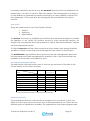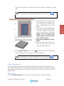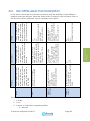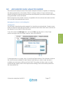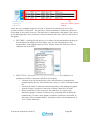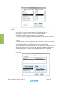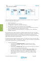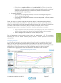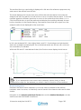
1
User manual v1.5.3 © Avacta Analytical Ltd 2012 Page 1 Avacta Analytical Optim 1000 v1.5 Issued By: Avacta Analytical Ltd 651 Street 5 Thorp Arch Estate LS23 7FZ UK +44 (0)844 414 0452 © 2012 Avacta Analytical Ltd All contents of this document are the property of Avacta Analytical Ltd. This document is the confidential work product of Avacta Analytical Ltd and no portion of this document may be copied, published, performed or redistributed without the express written authority of Avacta. © Avacta Analytical Ltd 2012 Page 1 CONTENT Avacta Analytical Optim 1000 v1.5 ....................................................................... 1 CONTENT ................................................................................................................... 3 HOW TO USE THIS MANUAL ...................................................................................... 5 PREPARATION ............................................................................................................ 7 I. SITE PREPARATION .................................................................................................... 7 System Components ................................................................................................... 7 Dimensions and weights ............................................................................................. 7 Environmental Requirements ...................................................................................... 8 Electrical Requirements............................................................................................... 8 Checklists...................................................................................................................... 9 II. SAFETY ADVICE ....................................................................................................... 11 General Instrument Safety ........................................................................................ 12 Electrical Safety ......................................................................................................... 13 Laser Safety ................................................................................................................ 13 Physical Hazards ........................................................................................................ 14 Chemical Safety ........................................................................................................ 15 Biological Safety ........................................................................................................ 15 Disposal ...................................................................................................................... 16 III. SOFTWARE INSTALLATION AND ACTIVATION ........................................................ 17 Your software ............................................................................................................. 17 Installing the Optim 1000 client software ................................................................. 17 Installing the Optim Analysis software ...................................................................... 21 Activating the analysis software............................................................................... 22 THE CLIENT SOFTWARE AND INSTRUMENT HANDBOOK ........................................ 23 IV. GETTING STARTED ................................................................................................ 25 V. POWERING OPTIM ON AND OFF ........................................................................... 27 Turning On Optim ...................................................................................................... 27 Turning on the PC ...................................................................................................... 27 Turning Optim Off ...................................................................................................... 28 VI. INTRODUCTION TO THE OPTIM CLIENT SOFTWARE ............................................ 29 Navigating the Software ........................................................................................... 29 File system................................................................................................................... 30 User Levels .................................................................................................................. 31 Structure Overview .................................................................................................... 31 VII. QUICK-START GUIDE ............................................................................................ 35 Quick-Start Outline .................................................................................................... 35 VIII. STARTING A NEW EXPERIMENT ............................................................................ 37 To Begin ...................................................................................................................... 37 Login ........................................................................................................................... 37 © Avacta Analytical Ltd 2012 Page 3 Projects ....................................................................................................................... 38 Samples ...................................................................................................................... 38 Experiments ................................................................................................................ 39 Runs............................................................................................................................. 40 Formulations ............................................................................................................... 40 Preparing the Micro-Cuvette Array (MCA) ............................................................. 45 Loading the MCAs into Optim .................................................................................. 46 Taking a Measurement ............................................................................................. 47 IX. USER MANAGEMENT ........................................................................................... 53 Users ............................................................................................................................ 53 X. DATA MANAGEMENT ............................................................................................. 55 Companies................................................................................................................. 55 Projects ....................................................................................................................... 56 Buffers and Additives ................................................................................................. 56 XI. EXPERIMENT SETTINGS ......................................................................................... 59 Experiments ................................................................................................................ 59 Temperature Control ................................................................................................. 60 Calibrations ................................................................................................................ 61 THE OPTIM ANALYSER HANDBOOK........................................................................ 65 XII. GETTING STARTED ................................................................................................ 65 A first look… ................................................................................................................ 65 Advanced mode....................................................................................................... 66 Choosing the analysis mode you want to use ........................................................ 68 XIII. THE OPTIM ANALYSIS PHILOSOPHY ..................................................................... 69 XIV. THE OPTIM ANALYSIS WIZARD ............................................................................. 71 Loading data into the wizard ................................................................................... 71 Performing Primary Analysis ...................................................................................... 72 Performing Secondary Analysis ................................................................................ 74 XV. ADVANCED DATA ANALYSIS MODE .................................................................. 77 Managing the software and Loading data ............................................................ 77 Primary Analysis .......................................................................................................... 82 Secondary Analysis.................................................................................................... 87 Generating a sample report..................................................................................... 94 XVI. EDITING AND DEVELOPMENT OF ANALYSIS METHODS ..................................... 97 The default methods ................................................................................................. 97 Creating and editing methods................................................................................. 99 Method management ............................................................................................ 103 Definition of standard functions included in the Optim Analysis software ......... 104 APPENDICES .......................................................................................................... 111 XVII. XVIII. RISK ASSESSMENTS.......................................................................................... 111 GLOSSARY OF TERMS .................................................................................... 118 © Avacta Analytical Ltd 2012 Page 4 HOW TO USE THIS MANUAL Welcome to the Optim 1000 Installation and Operation Manual. This section, believe it or not, is an instruction manual for your instruction manual. There are some useful pointers here so don’t despair! Take a minute to read this and the rest of the document will be easier to interpret. Software Instructions Avacta’s software provides the human-machine interface. You will soon learn to navigate it by instinct; but until you find your feet, some things to look out for in the software have been highlighted for you using the following code: Bold words indicate a tab or menu. Italics indicate a Menu Option. CAPITALS indicate a BUTTON. Direct instructions to the user are bullet-pointed for clarity, so you can scan the text and skip over the explanations if you wish. TIP – This symbol is used to inform the user of a shortcut or toolbar button Glossary At the end of the guide there is a Glossary of Terms which explains all of the jargon that appears in this guide. Throughout the guide text, a word that has a specific meaning for the Optim 1000 software for example a tab heading, is indicated by a capital letter at the start (for example, Project, Experiment, Run). It is advisable to look through the Glossary before beginning to use the instrument. Index To find information relating to a particular tab or topic, refer to the Index at the end of this guide. Instrument handling Watch out for the following alert words in the text, they will advise you of a physical hazard or an important step for you to carry out. The alert words indicate the particular level of observation or action, as defined below: IMPORTANT – Indicates information that is necessary for proper instrument operation or safe usage. © Avacta Analytical Ltd 2012 Page 5 CAUTION – Indicates a potentially hazardous situation that, if not avoided, may result in minor or moderate injury. It may also alert against unsafe practices. WARNING – Indicates a potentially hazardous situation that, if not avoided, could result in death or serious injury. DANGER – Indicates an imminently hazardous situation that, if not avoided, will result in death or serious injury. This is limited to only the most extreme situations. © Avacta Analytical Ltd 2012 Page 6 PREPARATION SITE PREPARATION This section of the manual describes how to prepare your site for installation of the Optim 1000 and how to get the instrument up and running. There are important safety warnings included here which must be observed by all personnel that have access to the instrument. Hardware installation should be completed before beginning the software. You should not unpack the instrument until the installation engineer is present. An Avacta Analytical qualified engineer should guide you through the site preparation and installation of the Optim 1000, so the following section is for information only. Before installing the Optim 1000 in the workplace, you need to prepare the site for installation according to the guidelines in this section. At the end of the section there are a set of checklists to help ensure that all the preparation tasks have been addressed. IMPORTANT - If the Optim Instrument is moved after it has been installed, it must be re-qualified by an Avacta service engineer before use. System Components The Optim 1000 consists of the following items: Main Optim 1000 unit External PC with keyboard and mouse Monitor Connector cables Dimensions and weights The dimensions and weights of a typical Optim 1000 system are given below. Ensure that the installation site can accommodate the dimensions and weights. Component Width Depth Height Weight Optim unit 85 cm (34”) 69 cm (28”) 76 cm (30”) 75 kg (165 lb) Desktop PC 17 cm* (7”) 43 cm* (17”) 37 cm* (15”) 10 kg* (22 lb) Monitor & Keyboard © Avacta Analytical Ltd 2012 Standard size Page 7 PREPARATION I. PREPARATION Clearances Once in operation, the main Optim 1000 unit needs at least 15 cm (6 inches) clearance on all sides for ventilation. For installation and on-site repair and maintenance, the Engineer will require at least 60 cm (24 inches) clearance either side of the instrument to gain access to the side panels. Cleaning your Optim Should you wish to clean your instrument after installation, you must first follow the shutdown procedure and switch off the unit at the mains. Wipe the exterior with a soft dry cloth or if necessary, a damp cloth with mild detergent. Environmental Requirements The site should be maintained under the following conditions. The user should be aware that fluctuations in environmental conditions can cause unexpected changes in the instrument’s performance. For best results, ensure that the temperature and humidity are maintained at a constant level. Condition Acceptable Range Temperature 15 to 30 C (50 to 95 F) Humidity 20 to 80 % relative humidity, non condensing This apparatus is for indoor use only. Under normal operation it has ingress protection rating IP20. The instrument should not be placed in direct sunlight. Electrical Requirements The main Optim 1000 unit requires connection to one standard mains socket. © Avacta Analytical Ltd 2012 Page 8 The Desktop PC requires connection to one mains socket. The monitor may require connection to one mains socket (or it may plug into the desktop PC). The Desktop PC will have its own standard power requirements. The main Optim 1000 unit is factory configured to operate interchangeably at ~120 VAC or ~240 VAC. Voltage Frequency Current drawn for Power consumed Fuse Rating Max. Power 220-240 V 50-60 Hz 0.5 – 1 A 2A 0.15 kW (VA) 110-125 V 50-60 Hz 1.25 – 2.5 A 4A 0.15 kW (VA) Over current protection >110% Checklists Check that the location fulfils the following criteria: The bench or table area is sufficiently large and can withstand the weights of the instrument. There are sufficient mains power sockets within range. The location of the instrument and computer allows for appropriate ergonomic usage. Check that all the following components are present: Optim 1000 analytical instrument Mains power lead USB lead Ethernet lead Desktop PC Monitor Mouse If your installation site is suitable and all of the Optim 1000 components are present, you are almost ready to begin! Your installation Engineer will set up the instrument for you so in the meantime, take the time to read the important safety information in © Avacta Analytical Ltd 2012 Page 9 PREPARATION IMPORTANT - In case of emergency, you must be able to immediately disconnect the main power supply to the instrument. the following section so that you can look out for those potential hazards when you begin to operate the instrument. PREPARATION © Avacta Analytical Ltd 2012 Page 10 II. SAFETY ADVICE The following table describes the symbols that may appear on Optim instruments. Each symbol may appear by itself or in combination with text that explains the relevant hazard. Symbol Description Indicates that you should consult the manual for further information and proceed with caution. Indicates the presence of an electrical shock hazard and to proceed with appropriate caution. Indicates the presence of a hot surface or other high temperature hazard and to proceed with appropriate caution. Indicates the presence of a laser hazard and to proceed with appropriate caution. Indicates the presence of moving parts and to proceed with appropriate caution. Indicates the presence of a biological hazard and to proceed with appropriate caution. Do not dispose of this product as unsorted municipal waste. Follow local municipal waste ordinances for proper disposal provisions to reduce the environmental impact of waste electrical and electronic equipment (WEEE). © Avacta Analytical Ltd 2012 Page 11 PREPARATION For your protection and to avoid malfunction of your Optim 1000, observe the following safety precautions. Read and understand all the information in the instructions for use and observe all warning and caution statements. Failure to do so may result in damage to the product, injury to personnel or poor instrument performance. PREPARATION General Instrument Safety The Optim 1000 was designed with due consideration of the Low Voltage, Electromagnetic Compatibility and Machinery Directives (2006/95/EC, 2004/108/EC and 98/37/EC respectively). It has been independently tested to EN61010-1:2001, EN61010-2-81:2002, EN 61326-1:2006, EN55022:2006 + A1:2007, EN5502:1998+A1:2001 +A2 2003, EN61000-3-2:2006, EN61000-3-2:2006, EMC-FCC: Title 47 of the CFR:2008 Part 15(b) (EMC requirements). Note: This equipment has been tested and found to comply with the limits for a Class A digital device, pursuant to part 15 of the FCC Rules. These limits are designed to provide reasonable protection against harmful interference when the equipment is operated in a commercial environment. This equipment generates, uses, and can radiate radio frequency energy and if not installed and used in accordance with the instruction manual, may cause harmful interference to radio communications. Operation of this equipment in a residential area is likely to cause harmful Interference in which case the user will be required to correct the interference at his own expense. Please be aware that any changes or modifications not expressly approved by the party responsible for compliance could void the user’s authority to operate the equipment. (FCC CFR 47 section 15.21). Moving and lifting the Instrument CAUTION - Physical Injury Hazard. Do not attempt to move or lift the instrument without the assistance of others, the use of appropriate moving equipment and proper lifting techniques. Improper lifting can result in painful and permanent back injury. Depending on the weight, moving or lifting an instrument may require two or more persons. IMPORTANT If the Optim Instrument is moved after it has been installed, it must be re-validated by an Avacta qualified service engineer before use. Moving and Lifting Stand-Alone computers and Monitors CAUTION - Physical Injury Hazard. Do not attempt to move or lift the computer or monitor without the assistance of others. Depending upon the weight of the computer and/or the monitor, moving them may require two or more people. Make sure you have a secure, comfortable grip on the computer or monitor when lifting. Make sure that the path from where the object is to where it is being moved is clear of obstructions. Do not lift an object and twist your torso at the same time. © Avacta Analytical Ltd 2012 Page 12 Keep your spine in a good neutral position while lifting with your legs. Participants should coordinate with each other before and during lifting objects. Electrical Safety The Optim 1000 instrument is classified as portable equipment. DANGER – Electrical Shock Hazard. Severe electric shock can result from operating the instrument without its panels in place. Do not remove the instrument panels. High voltage contacts are exposed when the instrument panels are not in place. Power DANGER – Electrical Hazard. Use properly configured and approved line cords for the local voltage supply. DANGER – Electrical Hazard. Continuous grounding circuitry is vital for safe operation of equipment. Never operate the instrument with grounding conductors disconnected. DANGER – Electrical Hazard. Plug the system into a properly grounded receptacle with adequate current capacity. Fuses WARNING – Fire Hazard. Improper fuses or high-voltage supply can damage the instrument wiring system and cause a fire. Before turning on the instrument, verify that the fuses are properly installed and that the instrument voltage matches the local power supply. DANGER – Fire Hazard. Replace fuses only with fuses of the type and rating specified for the instrument. Laser Safety CAUTION – Laser Hazard Use of controls or adjustments or performance of procedures other than those specified herein may result in hazardous radiation exposure. Optim is a Class I laser product. The lasers within the instrument have the following specifications. © Avacta Analytical Ltd 2012 Page 13 PREPARATION Ensure that everyone who operates the instrument has received instructions in general safety practices for laboratories and specific practices for the instrument. PREPARATION Wavelength Power output Pulse width/ Repetition rate Laser class 266 nm < 15 mW 1 ns/ ~6-10 kHz Class 4 473 nm < 20 mW CW Class 3B Danger to Eyes DANGER – Laser Hazard. Direct or indirect exposure of a laser beam to the eyes may result in permanent damage to the eyes, including photokeratitis, photochemical cataracts and retinal injuries. If operating the instrument without its covers, always wear appropriate laser protective eyewear. Hazard to Skin WARNING – Physical Injury Hazard. Direct exposure of a laser beam to the skin may cause erythema, melanoma, accelerated skin aging, increased pigmentation and photosensitive reactions. If operating the instrument without its covers, always wear appropriate personal protective equipment (gloves). Laser Warning Labels This label is displayed on the top of each of the left and right side panels of the instrument. Physical Hazards Moving Parts WARNING – Physical Injury Hazard. Moving parts can crush and cut. Keep hands clear of moving parts, including the motorised door, while servicing or operating the instrument. Hot Plate WARNING – Physical Injury Hazard. The plate where the samples are located may become hot during operation. Allow sufficient time for it to cool before moving or changing the samples. Workstation Safety Correct ergonomic configuration of the workstation can reduce or prevent effects such as fatigue, pain and strain. Minimise or eliminate these effects by configuring your workstation to promote neutral or relaxed working positions. © Avacta Analytical Ltd 2012 Page 14 CAUTION – Musculoskeletal and Repetitive Motion Hazard. These hazards are caused by repetitive motion, awkward posture, holding static unhealthy positions, contact pressure and other workstation environmental factors. Chemical Safety Chemical Hazard Warning WARNING – Chemical Hazard. Before handling any chemicals, refer to the Material Safety Data Sheet (MSDS) provided by the manufacturer and observe all relevant precautions. WARNING – Chemical Hazard. Chemicals in the instrument (including liquid in the lines) are potentially hazardous. Chemical manufacturers supply current Material Safety Data Sheets (MSDSs). These contain information on storing, handling, transporting and disposing of the chemicals safely. To minimize the hazards of chemicals: Read and understand the Material Safety Data Sheets (MSDS) provided by the chemical manufacturer before you store, handle or work with any chemicals or hazardous materials. Minimise contact with chemicals. Wear appropriate personal protective equipment when handling chemicals (for example, safety glasses, gloves, protective clothing). Minimise the inhalation of chemicals. Do not leave chemical containers open. Use only with adequate ventilation. Check regularly for chemical leaks or spills. If a leak or spill occurs, follow the manufacturer’s cleanup procedures. Comply with all local or national laws and regulations related to chemical storage, handling and disposal. Biological Safety General Biohazard WARNING – Biohazard. Your samples may contain components that have potential to transmit infectious diseases. Follow all appropriate local and national regulations. Wear appropriate protective eyewear, gloves and clothing when handling such samples. © Avacta Analytical Ltd 2012 Page 15 PREPARATION To minimize risks, use equipment that comfortably supports you in neutral working positions and allows adequate accessibility to the keyboard, monitor and mouse. PREPARATION The user must take responsibility for handling their samples in an appropriate and safe manner. The samples are contained with the MCA sample holders that are loaded into Optim. The samples should remain contained within these sample holders throughout the course of the experiments. Once removed from Optim, the samples and sample holders should be disposed of in an appropriate manner. Disposal Do not dispose of this product as unsorted municipal waste. Follow local municipal waste ordinances for proper disposal provisions to reduce the environmental impact of waste electrical and electronic equipment (WEEE). If the Optim unit is removed for disposal, the user should dispose of it in an appropriate manner. The Optim unit is made primarily from standard metal, plastic and electronic components. The WEEE regulations allow the onus for disposal of such equipment to reside with the user. The MCA sample holders may contain hazardous samples (if such samples have been run by the user). The user should follow appropriate local and national regulations for their disposal. © Avacta Analytical Ltd 2012 Page 16 SOFTWARE INSTALLATION AND ACTIVATION Your software The software is supplied in a package as shown below. The package contains two USB compatible devices, one which contains the installers for the software along with some documentation. The other is a security dongle to prevent unauthorised copying or distribution of the software. Each dongle is initially supplied in demo only mode and must be registered with Avacta Analytical before use. The software can be used for one month. If the software is not registered after this time then it will not be possible to use the software. To register and activate the software contact Avacta Analytical directly by emailing [email protected] supplying the serial number of your instrument, the date of installation, and who installed the instrument (either Avacta or one of our distribution partners). Installing the Optim 1000 client software It is only necessary to install the client software if you are upgrading from a previous software version. Your instrument will come supplied with the software pre-installed and you will only need to perform these steps if you have not obtained a controlling PC from Avacta Analytical, or if you reinstalling after a Microsoft® Windows® system failure. © Avacta Analytical Ltd 2012 Page 17 PREPARATION III. PREPARATION IMPORTANT - The Optim 1.1 database is not compatible with the v1.5 software. If you have upgraded your software it is not possible to load previously acquired data into the new version of the client software. As a result the run numbers will reset to 1. The old version of the software is still present on the system so this can be used as before but will not communicate with the instrument. Insert the memory stick into the desktop PC that is attached to the instrument. To install the Optim 1000 software v1.5 simply double click on the ClientInstaller.msi application. This will install the application onto the desktop PC that came with your instrument. The installation software will then start to install the Optim client software (and if you are updating, a new updated database also) onto your computer. The software will prompt you for a location to install the software. Select the default location, or choose a location of your own by clicking “Browse…” before clicking “Next >”. Once the software has been installed you will be prompted to configure the Optim Client 1.5. To do this, click “Next >” in the window below. © Avacta Analytical Ltd 2012 Page 18 PREPARATION You will then need to enter the hostname of the instrument that you are connecting to. If you are installing the software on a PC supplied with an Optim 1000 instrument by Avacta Analytical then this should be automatically populated with a valid hostname. Otherwise, you will need to enter this here. The hostname you require will be AVAOPT-xxxx where xxxx are the last four digits of your instrument serial number. © Avacta Analytical Ltd 2012 Page 19 The installation software will then install the Optim Client 1.5 database. You will not need to interact with the installer during this time. Once completed, a series of shortcuts will appear on your desktop. These shortcuts will help you use the Optim Client software efficiently. PREPARATION Optim.Client 1.5 – this is the software itself. Double clicking on this will start the software and begin communication with the instrument Edit formulation – this will allow you to edit the formulation information Optim Manual – this is the user manual for v1.5 of the Optim instrument Optim Quick Start Guide – a simple and quick way to get started using Optim Export 1.5 – where files exported from the client software are saved Import 1.5 – the source of formulation information for importing DO NOT USE THE FOLLOWING UNLESS DIRECTED TO BY AN AVACTA REPRESENTATIVE: Optim Reset 1.5 – a tool used to restart sub components of the Optim instrument Database Config Tool – a tool to change the default parameters in the instrument After this process has successfully completed and if you are upgrading from a previous software installation then double click on “Optim_1_5_update.exe” to update the Optim instrument you are connecting to. Again, you will need to enter the target instrument that you wish to update. © Avacta Analytical Ltd 2012 Page 20 Installing the Optim Analysis software Avacta Analytical has developed a new analysis tool, incorporating foundation technology called Igor Pro v 6.2 from Wavemetrics Inc. To install the Optim Analysis software v 1.5 simply extract the contents of the Optim Analysis zip from the memory stick, and double click on AnalysisInstallerFull.msi application. This will install the subroutines, preferences files and the Igor Pro package onto your computer. In order to use this software you must have a dongle for each computer on which you wish to use the software. You may install the software on one computer only, and any subsequent installations will require you to purchase an additional licence and dongle from Avacta Analytical. The Optim Analysis software loads and saves data from defined folders on the installed computer. The default locations are configured such that raw data (in the form of spectra saved by the client software) is loaded from: C:\Optim.Client\Database\OptimDB\Files\Capture Data that is stored in studies are by default saved in a folder called “Optim Studies” that can be found in the users Documents folder, and accessed either directly or via a shortcut on the desktop. If you are installing the analysis software on a computer that is not connected to an instrument and you wish to load data from a different location please refer to later sections which provide information on how to achieve this. © Avacta Analytical Ltd 2012 Page 21 PREPARATION IMPORTANT - It is essential that the device installer is executed on the supplied desktop PC and that the Optim user is logged into the system at the time the installer is run, otherwise installation will fail due to insufficient permissions. Activating the analysis software The analysis software features a copy protection dongle that requires initial activation before analysis can be saved or exported. PREPARATION To activate the software select the OptimAnalysis menu and the Update Licence option. You should then contact Avacta Analytical Ltd via [email protected] with your name, Optim serial number, the dongle number and the number of activations shown above. Avacta Analytical will send an activation code that will enable you to use the software without limitations while the dongle remains inserted. If you remove the dongle you will not be able to save or export data from the software. © Avacta Analytical Ltd 2012 Page 22 The purpose of the Client software Handbook is to guide a user through the day-today operation of Optim 1000. “Starting a New Experiment” guides the Analyst user through every step of the settings and options that are involved in running a new experiment. Sections in the analysis segment of this chapter introduce the user to loading and processing data after it has been acquired. Some settings are hidden from the Analyst user and must be set up by the Administrator. For instructions on those features that are exclusive to the Administrator, and for in-depth descriptions of the pre-programmed software routines such as calibrations and analysis macros, read the later sections that appear later in this handbook. The purpose of these later sections is to guide an Administrator-level user through the additional features of the software and to give further information about the default settings and options. Here you will find detail about the calibration functions applied to the raw data, the logic of the temperature control feature and some other useful information. The administrator information is arranged into three sections: User Management, Data Management and Experiment Settings. © Avacta Analytical Ltd 2012 Page 23 CLIENT SOFTWARE AND INSTRUMENT HANDBOOK THE CLIENT SOFTWARE AND INSTRUMENT HANDBOOK IV. GETTING STARTED This section contains all the information you need to get started with the Optim 1000 instrument and its accompanying software, including how to power the instrument on and off safely. The Optim software will already be installed on the PC. In this part of the guide you will find information about the screen layout, the user access levels and an overview of how the software manages data. For quick reference, Section VII has a quick-start guide, which summarises the main steps involved in making a measurement with Optim 1000. There is also a flowchart to demonstrate the typical decisions taken by a user during the measurement process. IMPORTANT - For safe operation of the instrument, the user is advised to follow the instructions and guidelines given in this document. DANGER - The user should NOT remove any of the panels on the instrument. With the instrument turned on and the side panels removed, there is a significant risk of exposure to potentially harmful laser radiation, high voltage electricity and hot surfaces. The service engineers may need to remove these panels whilst operating the instrument. They should assess the Risks associated with the Hazards, and take appropriate action to reduce these Risks to an acceptable level. A set of risk assessments for the user are provided in the appendix of this document. © Avacta Analytical Ltd 2012 Page 25 CLIENT SOFTWARE AND INSTRUMENT HANDBOOK Please note that the Optim Client software can only be supported on the PC connected to the Optim 1000 and should not be installed or copied onto any other computers. V. POWERING OPTIM ON AND OFF Turning On Optim Optim 1000 has two power switches: 1) Firstly, at the top of the rear panel, where the power and data leads enter Optim, a rocker switch controls the overall power to the instrument. IMPORTANT - Once this switch is set to On (1), all safety precautions should be observed. 2) The second power switch is located on the front of the instrument above the service status LEDs. Press this button once to start the Optim 1000 onboard computer. The UV laser reaches optimal stability after one hour of warm up time. Turning on the PC The accompanying desktop personal computer is controlled independently of the Optim 1000 instrument. The computer can be used without the instrument being on, but not vice versa. Please refer to the PC manufacturer’s manual for instructions on how to turn on the PC. Automatic System Checks When the Optim 1000 has been turned on, the service status LEDs (towards the top right of the front panel) will indicate the status of the constituent sub modules. When Optim has been completely switched on and has booted up, six of the indicator LEDs on the front panel should become green. The central LED should © Avacta Analytical Ltd 2012 Page 27 CLIENT SOFTWARE AND INSTRUMENT HANDBOOK Switching this on will activate the power to the internal sub modules, including the laser sources. change to amber. IF ANY OF THE LEDS REMAIN RED, CONTACT YOUR SUPPORT AGENT. Turning Optim Off IMPORTANT It is advisable to switch off both the Optim 1000 and the accompanying PC when not in use. 1) Shut down the onboard computer by selecting menu. shutdown from the file CLIENT SOFTWARE AND INSTRUMENT HANDBOOK The blue light on the power switch (upper right of the front panel of the Optim 1000) should turn off after a few minutes. 2) 3) Turn off the main power using the rocker switch near the back left of the instrument. The external PC may be used after Optim has been turned off. When shutting down the software, always use File - Exit. © Avacta Analytical Ltd 2012 Page 28 VI. INTRODUCTION TO THE OPTIM CLIENT SOFTWARE Navigating the Software IMPORTANT software. Always switch the Optim 1000 fully on before starting the CLIENT SOFTWARE AND INSTRUMENT HANDBOOK The Optim 1000 client software controls the system during a measurement and then processes the measurement data through a series of calibration functions. A typical screen is shown below. The menu bar gives access to the open/close Run, logout and shutdown features as well as providing a quick-look list of the acquisition and analysis functions. This manual can be found in .PDF format via a link in the Help menu. The toolbar contains a selection of the most-used buttons to allow the user to quickly set up a measurement, collect data and process the results. These are summarised in the table below: Symbol Action Shutdown Optim. Log the user out of the Optim client program. Open the door to load samples into Optim. Close the door and return the stage to its start position. Acquire a single shot (this will not be saved to the database). © Avacta Analytical Ltd 2012 Page 29 Symbol Action Start a Run (acquired spectra are saved to the database). Abort the Run (you will lose the current settings). The TIP symbol in this guide indicates that a toolbar button or menu option can be used as a shortcut. CLIENT SOFTWARE AND INSTRUMENT HANDBOOK The tabs are arranged in roughly chronological order so that a user works from left to right when setting up a new experiment, taking a measurement, viewing the data and performing analysis. Hover over a tab heading for a description of the tab contents. Some buttons and features also have handy tooltip pop-ups to give you a snippet of useful information. The status bar at the bottom of the window displays the following information: The user that is currently logged on The Project that is currently in use The selected Experiment The ID and title of the active Run The MCA configuration (number of wells in the current Run) Live status updates about the Optim 1000 instrument and a progress bar File system Database The Optim software has an inbuilt database system that stores all newly acquired data sorted by Project, Experiment and Run. Within the software, data can be loaded by the Run ID and viewed, and all the results generated will automatically be saved to the database. Exporting and Importing Data can also be exported from the program. Any raw data, calibrated data or analysis results will be exported in the Excel format. Exported files will appear in a list in the Results tab and can be accessed in the folder C:\Optim.Client\Export. IMPORTANT It is advisable to save exported files immediately in a different file location as the Export folder will be cleared each time the software is restarted. © Avacta Analytical Ltd 2012 Page 30 Formulation details for the MCAs can be imported from Excel into the database. The easiest way to do this is to use the “Edit Formulations” file that appears as a shortcut on the desktop to generate formulation information. It is also possible to import files from elsewhere on the hard drive by entering the file path details in the import window. User Levels There are three levels of user in the Optim software: The Analyst user-level is a simplified user-interface that has been designed to enable an operator to use Optim, but restricts access to more advanced features. An Analyst user can prepare and load samples into Optim, take measurements, analyse results and generate reports. A Project Supervisor has the same access level as an Analyst user except that they are able to create a new Project and manage the user access to that Project. The Administrator user-interface allows access to the user management area and includes advanced Data management in addition to all of the functions that are available to the Analyst and Supervisor users. User tab access in Optim software The table below indicates which level of user can access each of the tabs in the current version of the Optim software. User level TAB Analyst Project Supervisor * 1) Login 2) Users 3) Companies 4) Projects * 5) Experiments 6) Samples 7) Runs 8) Formulations 9) Measurements 10) View Spectra * User has limited access to the features of this tab Administrator Structure Overview The Administrator defines a user identity and assigns a list of projects to that user. Within a Project, the user must choose one of the experiments to run. There are four different types of experiment available. The experiments contain pre-programmed © Avacta Analytical Ltd 2012 Page 31 CLIENT SOFTWARE AND INSTRUMENT HANDBOOK 1. Analyst 2. Supervisor 3. Administrator settings designed around characterising certain properties of samples for typical Optim applications. The diagram below is a simplified view of the structure of the software. At first glance this may appear complex, but many of the processes illustrated here are default settings that the user need not be concerned with. Further detail on all of the stages depicted can be found further on in the manual if you stay awake to read that far. A more experienced user can use the diagram to understand how settings and data are handled by the software. CLIENT SOFTWARE AND INSTRUMENT HANDBOOK Square-edge boxes represent processes that happen automatically, whereas roundedge boxes indicate that the user must interact with the software in some way. In this diagram, the term “user” includes all levels of user. Please refer to the Glossary at the end of this guide for other definitions. © Avacta Analytical Ltd 2012 Page 32 © Avacta Analytical Ltd 2012 Page 33 CLIENT SOFTWARE AND INSTRUMENT HANDBOOK VII. QUICK-START GUIDE Quick-Start Outline Here is a brief summary of how to obtain stability information about your molecule of interest using the Optim 1000. Turn on Optim, first by the switch at the back, then the button at the front. Switch on the PC. Allow at least one hour for the laser in the instrument to warm up. When all the lights at the front of Optim are no longer red, open the Optim Client 1.5 software and Login to a Project. Select an Experiment to start a new Run. Decide the MCA configuration (number of wells) you wish to use and input the Formulation details for your Samples. Fill the micro-cuvettes with the formulations. Open the door, pull out the tray and load the Micro-Cuvette Arrays (MCAs) onto the hot plate, starting from the left. Place the lid on the copper plate. Push the tray in and Close the door. View the Measurement details, amend the temperature step settings and start the Run. View the calibrated spectra in the View Spectra tab as they are acquired. When the Run is finished, go to the Optim Analysis software to begin analysing the data and load the run. Perform Primary Analysis to produce a set of unfolding curves and scatter data. Perform Secondary Analysis to find the equilibrium midpoint of the unfolding curves and the temperature of aggregation onset. Compare these results to find the more stable formulations for the molecule of interest. When finished, Shutdown Optim using the software. Wait until all the lights go red and the blue light goes off. Then it is safe to turn off the switch at the back. Use the menu option File Exit to close the Optim Client Software. Save any exported files in a new folder. Shutdown the desktop PC. If pictures are more your thing, overleaf is a flowchart which guides the Analyst user through this process. Simply follow the arrows and make a decision anytime you reach a blue diamond. © Avacta Analytical Ltd 2012 Page 35 CLIENT SOFTWARE AND INSTRUMENT HANDBOOK CLIENT SOFTWARE AND INSTRUMENT HANDBOOK Page 36 © Avacta Analytical Ltd 2012 VIII. STARTING A NEW EXPERIMENT This part of the manual covers the basics of operating the instrument. It includes all details that are relevant to an Analyst-level user to step them through the process of loading samples into the Optim 1000 instrument, making a set of measurements, analysing the results and producing a report. The more challenging task of interpreting the results will be left to a more knowledgeable scientist-type person and will not be discussed in this manual. To Begin Ensure that Optim is switched on: You should see a ring of blue LEDs and a row of green lights on the front of the instrument (one may remain amber until the software is started). If some or all of the lights are off, please refer to Section I for instructions on how to power up the instrument. Start up the Optim 1000 Client software by double clicking the link on the PC desktop – the Login tab should be displayed. The software cannot be run when the Optim instrument is switched off. Login The Analyst’s login details will be set up by the Administrator. The Administrator (or Project Supervisor) also has control over which projects are available to Analyst users. Insert your username and password. Choose a Project from the drop-down list. Click LOGIN. © Avacta Analytical Ltd 2012 Page 37 CLIENT SOFTWARE AND INSTRUMENT HANDBOOK Before an Analyst can start a new experiment, the Administrator must set up the new user’s login details and create a Project in the database. Projects To view the description of a Project or to change to another Project after you have logged in, use the Projects tab. CLIENT SOFTWARE AND INSTRUMENT HANDBOOK In the list on the left, click on the Project you wish to work on. All the settings and data for that Project will then be loaded. If you have been assigned the responsibility of being a Project Supervisor, you can edit the details of the Project. You also have permission to create a new Project. Samples This tab contains information about the samples that will be investigated as part of the selected Project. Only samples relevant to the selected Project will be listed here. Any samples listed on this tab will also appear in a drop-down list in the Formulations tab. To add a new Sample to a Project: Click NEW. In the window on the right, type in a sample Name (ID) and brief Description. These will appear in the list of Samples on this page and in © Avacta Analytical Ltd 2012 Page 38 Click SAVE. Any Samples associated with a given Project will be listed by Name in the Formulations tab drop-down list, which will be discussed later. Experiments The user is provided with four templates for experiments (listed below). Within a Project, any or all of the experiments can be performed. Each of the templates has predefined settings that are suitable for typical Optim applications. These are described in further detail in the Method box on this tab and in Section XI on page 59 of this handbook. Choose an Experiment template by clicking once on one of the four options: In the pop-up box: © Avacta Analytical Ltd 2012 Page 39 CLIENT SOFTWARE AND INSTRUMENT HANDBOOK the drop-down menu on the Formulations tab. [Note: The description field has a character limit and will be highlighted in red if the description is too short.] All other information is optional. You can record the Lot No., Concentration, Appearance, Molecular Weight and Expiry date in this window. If your sample has been supplied or manufactured by another company, select the appropriate companies from the drop-down lists at the bottom of the window (the list of companies will be managed by the Administrator). o o Click NEW to start a new Run, Or, to view historical data, choose a Run from the drop down list and click LOAD. The Optim software will now load the settings for the chosen Experiment. Runs This tab shows a list of all completed runs for the chosen Experiment in the selected Project. Click on a Run to view the details in the box on the right of the screen. If you are beginning a new Run, it will appear at the bottom of the list. CLIENT SOFTWARE AND INSTRUMENT HANDBOOK If the most recent Run is not already highlighted, click on it and click EDIT to edit the title and description of the Run you are about to start. Note down the Run ID highlighted in red at the top of the Run Details window. This ID can be used to find the Run again quickly using the Open Run command in the File menu, and will be used in the data analysis. Choose the MCA configuration (the number of formulations in the Run) using the drop-down list. The Device selection should show the default Optim version. Click SAVE. When you have filled in the Run details, go to the Formulations tab to fill in the data about the contents of the micro-cuvettes. Formulations This tab is designed to store all the information about the contents of the microcuvettes in the current Run. Data can either be input directly to the database, or imported from Microsoft Excel. The Excel file must be in the correct format to be compatible with the Optim software. You should see an empty table with the same number of rows as there are wells in the MCA configuration you have chosen. © Avacta Analytical Ltd 2012 Page 40 CLIENT SOFTWARE AND INSTRUMENT HANDBOOK To input formulation data to the database manually: In the Formulations box, highlight the well you wish to edit and click NEW. (If you wish to change data that has already been entered, click EDIT). In the Formulation Details box, fill in the following information for each well that contains a sample. Standard Data: © Avacta Analytical Ltd 2012 Page 41 o o o o Well Sample Name: Write a brief description of the formulation in the selected well. This will be displayed in the list of acquired spectra and results. Well Sample Ref.: This reference is for the user only and should be chosen according to the user’s company policy. Sample: Select a sample molecule from the drop-down list and enter the concentration (in mg/ml). Buffer: Select a buffer from the drop-down list and enter the concentration (Molar, M). Administrators can add to the list of buffers via the Samples tab. For instructions, see section X on page 55. o Analyse: Tick the tick-box to include this well in the analysis stage. CLIENT SOFTWARE AND INSTRUMENT HANDBOOK Optional Data: o pH: Type in the pH for this formulation. o Replicate No.: Keep a record of duplicate formulations by labelling them with the same replicate number. o Additives: To add an additive to the formulation, click NEW, select an additive from the drop-down list and type in the concentration (Molar, M). Click SAVE. The additive will now be listed (Highlight an additive in the list and use the buttons below to EDIT or DELETE it as required). Administrators can add to the list of additives via the Samples tab. For instructions, see section X on page 55. When you have entered all the required information, click SAVE. If you wish to use this list of formulations again, there is an option to EXPORT the data to an Excel file (located in C:\Optim.Client\Export). To import formulations you have previously edited and exported: Note the filename that you used to EXPORT the data to an Excel file (located in C:\Optim.Client\Export). Change the path in the spread sheet directory to reflect where you exported the formulation too before. Click IMPORT. To import formulations from Microsoft Excel: Open the shortcut “Edit Formulation” on the desktop to open the Excel tool. If you see a Security Warning at the top of the window in Microsoft Excel, click Enable Content before continuing. © Avacta Analytical Ltd 2012 Page 42 You will be presented with an Excel sheet called “Project samples”. Change the number of samples from 3 to match the number of samples you have on the Samples tab in the client software. Add any new samples to the Sample tab Note the example contained here has a deliberate mistake in the missnaming of Rituximab in Excel template formulation editor. If such an error occurs in practice the user will be presented with an “Error no sample record named ‘Rituzimab’ found for well no. 1” warning. (Please note: the Sample Name is case sensitive and must exactly match the name in the database.) Proceed onto the Create Formulation sheet. Choose the correct MCA configuration and the Number of additives from the dropdown boxes at the top of the sheet – the sheet should expand or contract to show the relevant cells for editing. [Note, due to limitations imposed by Microsoft, when using the Excel import template it is possible to enter up to three additives per sample well. If you wish to use more you must add them using the manual method outlined above.] For each sample, select an entry for the Sample Name using the dropdown box at the side of each cell, and complete the rest of the formulation information. If you wish to perform a buffer background measurement (for example if you have fluorescing compounds in your buffer) the analysis software © Avacta Analytical Ltd 2012 Page 43 CLIENT SOFTWARE AND INSTRUMENT HANDBOOK CLIENT SOFTWARE AND INSTRUMENT HANDBOOK will attempt to find the spectra for the relevant buffer and subtract it from the sample spectra automatically. To do this: o Enter identical formulation information in the well in which the buffer will be loaded, but leave the Sample Details column empty. o Change the reference column entry to TRUE. o Changing the Analyse column entry to FALSE will not affect the buffer subtraction, but the buffer spectra will not be analysed. It will not be possible to see how the buffer fluorescence and light scattering signals change with temperature. If you are measuring replicates, insert a value into the Replicate No column, all rows with the same replicate number will be grouped together as replicates in the Optim Analysis software. Type in a filename and click CREATE FORMULATION. A file will be created in the Import folder. In the software, go to the Import/Export box and input the Excel file name and location. Click IMPORT. An example formulation editor sheet is shown below. In this case, there are two sample molecules, Rituzimab [sic] and Trastuzumab. The following points are worth noting about this formulation: 1) There are four duplicates (the first eight formulations) a. A1 and C1 b. B1 and D1 c. E1 and G1 d. F1 and H1 2) There are four buffers being measured a. M1 is the buffer for A1 and C1, and at each temperature the spectrum of M1 will be subtracted from that of A1 before analysis. The spectra of M1 will not be analysed b. N1 is the buffer of F1 and H1, with a comparable outcome as above c. O1 is the buffer for I1, and at each temperature the spectrum of O1 will be subtracted from that of I1 before analysis. The spectra of O1 will be analysed © Avacta Analytical Ltd 2012 Page 44 d. P1 is the buffer for L1 Now would be a good time to fill the micro-cuvettes with the sample formulations and check them against the list displayed on your screen. The next two sections will describe how to prepare and load the micro-cuvette arrays (MCAs). Preparing the Micro-Cuvette Array (MCA) CLIENT SOFTWARE AND INSTRUMENT HANDBOOK For making measurements with the Optim 1000, the user can purchase a quantity of Micro-Cuvette Array sample holders (MCAs). Preparation of samples for use in Optim is not covered in this document. For further information about how to handle the sample holders, please read the MCA User Guide. Warning! - Take care not to touch the surface of the quartz cuvettes as this could significantly degrade the quality of the data. 1) Either use a single-channel pipette or preload the formulations into a row (e.g. A9-P9) of a microtitre plate, such as a conical well, low volume, 384 well plate (image: Starlabs E1042-3849). © Avacta Analytical Ltd 2012 Page 45 2) Place the black cuvette holder with pre-loaded cuvettes into the groove on the Filling Tool, so that it is held in place by the magnets. 3) Use a single or 16-channel micropipette, with an appropriate volume range, to collect the sample formulations from the pre-loaded row in the microtitre plate or sample vessel. Item no. 1022 4) Align the pipette tips with the microcuvettes using the grooves in the Filling Tool, indicated by an arrow in the illustration. CLIENT SOFTWARE AND INSTRUMENT HANDBOOK 5) Gently press the plunger, ensuring that the formulations flow into the microcuvettes. 6) Place one seal, in the correct orientation*, into each side of the blue frame. These will seal the ends of the cuvettes and ensure that the formulations do not evaporate at high temperatures. *1 µl *The round side of the seal should be in contact with the ends of the 1 µl cuvettes. The square side is used to seal the ends of the 9 µl cuvettes. 7) Slide the frame onto the cuvette holder, ensuring that the tongue and groove fittings mate correctly at each end of the black holder. *9 µl 8) Gently lift the MCA off the Filling tool and close the hinged part of the cap, mating the tongue and groove near the clip. Apply gentle pressure to compress the seals against the ends of the cuvettes and secure the cap with the clip. WARNING – Biohazard/Chemical Hazard. Your sample formulations may contain components that have potential to transmit infectious diseases or are dangerous chemicals. Follow all appropriate local and national regulations. Wear appropriate protective eyewear, gloves and clothing when handling such samples. Loading the MCAs into Optim Open the Measurements tab. In the Stage Control window, click OPEN DOOR to access the sample drawer. This will open the door and © Avacta Analytical Ltd 2012 Page 46 move the stage into a position where it is easily accessible from the door. 1) Wait for the door to open fully and then pull the drawer out to its full extent. The LED will flash intermittently red and green. 2) Place the MCA sample holders onto the hot plate sequentially from left to right, ensuring that each is secured by the brass spigots and that each is flat with no gap between the MCA base and the copper. 3) Place the insulating lid over the MCAs. 4) Push the drawer all the way back in and check that the door LED flashes green. In the Stage Control window, click CLOSE DOOR to close and lock the door and return the stage to its default position. TIP – Alternatively, click the CLOSE button on the Toolbar. Taking a Measurement The chosen Experiment will have default settings for the measurements that the instrument will perform (for example, UV fluorescence). There is no need to change any settings at this stage, as the defaults have been chosen to be suitable for most applications. Measurements View the Measurements tab to see which measurements will be performed. © Avacta Analytical Ltd 2012 Page 47 CLIENT SOFTWARE AND INSTRUMENT HANDBOOK TIP – Alternatively, click the OPEN button on the Toolbar. CLIENT SOFTWARE AND INSTRUMENT HANDBOOK If you wish to change the default exposure time, slit width or centre wavelength: In the Measurement Settings window, click EDIT. Type in the required exposure time, slit width and centre wavelength. Click APPLY to apply the changes. It could take several seconds to apply the changes. Temperature Control The Temperature Control window displays the temperature settings that have been chosen for this Experiment: Status: This tab displays the temperature, hold time and step count status throughout a Run. Ramp Settings: For a “thermal ramp” type Experiment, the temperature will start at the Start Temperature and a measurement will be taken for each well of the MCA configuration. The temperature will then increase by the chosen increment size (indicated by Temp Step). When the set temperature of the copper plate has been reached, the instrument waits for the designated Temp Hold Time and then takes another set of measurements. Measurements are taken at each temperature step until the Stop Temperature has been reached. © Avacta Analytical Ltd 2012 Page 48 Click EDIT. Type in a Start Temperature and Stop Temperature within the range from 15 °C to 100 C. Type in the required Temperature Step Size (C) and Hold Time (seconds). Click APPLY to apply the changes. Isothermal Settings: For an “isothermal” type Experiment, the temperature remains constant within a tolerance of less than half a degree over the full range of operating temperature. Measurements are taken at each well and then the instrument waits for the designated Wait Period before beginning a second set of measurements. This process is repeated for the number of times indicated by the Repeat Count. To alter the Isothermal settings: In the Isothermal settings tab, click EDIT. Type in the required Temperature (between 15 °C and 100 C), Wait Period (seconds between measurements) and Repeat Count number. Click APPLY to apply the changes. Linear Ramp: For a thermal unfolding using a linear heating ramp profile type Experiment, the temperature increases from a Start Temp to a Stop Temp at a constant rate that is defined by the user by Rate. All the samples are heated in the same way and at each point in time are at the same temperature. Measurements are taken at each well sequentially. After each spectrum is acquired, before moving to the next well the system waits for a period of time given by Well Hold Time. This © Avacta Analytical Ltd 2012 Page 49 CLIENT SOFTWARE AND INSTRUMENT HANDBOOK To alter the Ramp settings: value can have a minimum value of 15 seconds, as any shorter value can lead to a break down in the linearity of the heating rate. To alter the Linear Ramp settings: In the Linear Ramp tab, click EDIT. Type in the required Start Temperature and Stop Temperature (between 15 °C and 100 C), Type in the required Well Hold Time (seconds between measurements of adjacent wells) and Rate. Click APPLY to apply the changes. CLIENT SOFTWARE AND INSTRUMENT HANDBOOK Stage Control The Stage Control window displays the MCA configuration that has been chosen for the Experiment, which should be the same as the MCAs you have loaded onto the stage. During a Run, the stage moves the focus from well to well and measurements are taken at each one. As each well is measured, it will be highlighted in this window. TIP – NEW FEATURE – clicking on a well will move the instrument optics such that the selected well becomes the active well. A single shot will now capture the selected well. Run Control The Run control window contains the buttons to take a single shot, start a Run or abort a Run. If a Run is aborted before completion, the partial set of data will still be saved to the database. If you wish to restart the Run, you must opt to start a New Run from the Experiment menu and re-enter all of the settings as required. (The Run settings have been recorded in the .xml file which can be accessed by clicking on the blue ID of a Run in the View Spectra tab.) When you have checked or changed the measurement settings: You can verify your settings by taking a single snapshot (of each well) to preview the spectrum. Click window. © Avacta Analytical Ltd 2012 SINGLE SHOT in the Run Control Page 50 TIP – Alternatively, select Single Shot from the Acquisition menu or use the toolbar button. The acquired spectrum will be immediately visible in the View Spectra tab, but will not be saved to the database. If you wish to save a copy of this spectrum, you can export the data (calibrated or raw) to Excel using the EXPORT button or by right-clicking the spectrum in the list. To begin a run, click START RUN in the Run Control window. All spectra collected during a run will be saved to the database automatically and can be accessed at any time by selecting the appropriate Project Experiment Run. TIP – Alternatively, select Start Run from the Acquisition menu or use the toolbar button. View Spectra In this tab, the user can view any of the spectra that have been acquired in the selected Run. These spectra have already been calibrated using the default calibration procedures. To view details of the calibration procedures see later in this manual. If you have loaded a Run and there are no spectra listed in the View Spectra tab, click LOAD in this window and wait a few seconds for the list to be populated. Click on any spectrum to view it as a graph or © Avacta Analytical Ltd 2012 Page 51 CLIENT SOFTWARE AND INSTRUMENT HANDBOOK Tick the Auto Show Spectra box to view the most recently acquired spectrum. Change the view settings by typing values into the min and max boxes to the left of the graph, then selecting a different field. Sort the data by clicking on a column heading. Hold down shift and click up to four column headings to sort by multiple factors. You can export data from this tab to Microsoft Excel files. All exported files will be saved in the folder C:\Optim.Client\Export. The spectra displayed will have been calibrated by default using the four calibration procedures described. To export a calibrated spectrum to Excel before performing any analysis: CLIENT SOFTWARE AND INSTRUMENT HANDBOOK Right click on the spectrum in the list and choose Export Calibrated Spectrum. A subset of spectra can also be exported by well, temperature, measurement or all spectra can be exported to Excel. To export many spectra: Click the EXPORT button. Clicking an option in this window will send an exported file to the designated folder. Close the dialogue box when you are finished by clicking the cross in the top right hand corner. You can also opt to export the raw data. Raw data is data collected directly from the CCD camera without wavelength, device response or background corrections having been applied. Raw data is always stored in the database so that the user can load an old set of data and export the raw file at any time after the acquisition. To export raw data: Right click on the spectrum in the list and choose Export Raw Spectrum. Alternatively, click the EXPORT button. In the dialogue box, select a single spectrum to export or click Export All Raw Spectra. Close the dialogue box when you are finished by clicking the cross in the top right hand corner. To download the .xml file: Click on the blue ID of any of the spectra listed to open an external dialogue box with the options to open or save the file. These files will be in an open .xml format, which contains all raw data, calibrated data and a header listing all the settings of the instrument at the time of acquisition. Any files accessed via these links will be saved in C:\Users\...\Downloads. © Avacta Analytical Ltd 2012 Page 52 IX. USER MANAGEMENT Users CLIENT SOFTWARE AND INSTRUMENT HANDBOOK This tab allows the Administrator logged into the “Optim Demo” to add users to the database, define the permission levels of the user and assign projects to the user. New Users To create a user: In the Users tab, you will see a list of the users in the left hand window. At the bottom of the window, click NEW. You will be prompted to enter a username for the new user. Enter the new user’s personal details in the User window. In the Login box at the bottom you can edit the username and create a password for the new user (these are not case-sensitive). Click SAVE to save all the changes on this page. Assigning Projects to Users When assigning a Project to a user you must decide the user’s level of access for each Project. It is advisable to have just one “Supervisor” for each Project and to assign all other users to the default “Analyst” access level. A Project Supervisor will be able to edit the details of the selected Project and grant access to other users but can also create, edit and delete their own projects. An Analyst level user can merely work on the Project and view its details. To assign a Project to a User: In the Projects window of the Users tab, highlight a Project in the righthand list and click ADD. The Project will appear in the Allocated Projects list on the left of this window. The default access level for a user is Analyst. Define the user’s access level by selecting the Project and clicking EDIT in the access level box. © Avacta Analytical Ltd 2012 Page 53 Choose either Analyst or Supervisor from the drop down list. Click SAVE in this window. Click SAVE to save all the changes on this page. Listed users can be edited, deleted or disabled. The Administrator will always be able to see a full list of the users and make changes to the list. Deleting or Disabling User Profiles On the occasion that you want to remove a user from the database, there are two options: to disable or delete the user. Disabling a User: CLIENT SOFTWARE AND INSTRUMENT HANDBOOK To maintain access to the user’s details but stop them from logging in, simply disable the login for that user by ticking the Locked box on their profile. Their name will still appear in the list of users but their login details will be disabled so that an error message appears if the user tries to log in. Deleting a User: Highlight the user’s name in the list and click DELETE. This will deactivate the user so that their name is removed from the list of users and you will no longer be able to access their profile. Any data that the user collected will still be accessible by other users through the Project database. © Avacta Analytical Ltd 2012 Page 54 X. DATA MANAGEMENT In the Optim Client software there are two types of data: Global and Projectspecific. Most of the data that an Analyst-level user encounters is Project-specific. However, the Administrator can also change Global data. The list of users is an example of Global data. The database contains a list of users as created by the Administrator. When logged in, the Administrator can always edit and view the full list of users. Similarly, the Companies, Projects, and Buffers and Additives sections contain Global data. The following sections describe how the Administrator might use each tab to manage their data. Companies This tab allows the Administrator to keep a record of the companies that are associated with an investigation, for example, companies that provide samples or experiment templates. As a default, Avacta Group PLC will be listed. An important function of this list is to identify the source of bought samples in the database. To add a company: Click NEW. Fill in the name and details of the company in the window on the right. Click SAVE. This company will now be listed in a drop-down list on the Samples tab so that their records can be kept on the database. © Avacta Analytical Ltd 2012 Page 55 CLIENT SOFTWARE AND INSTRUMENT HANDBOOK Samples and Experiment Runs are examples of Project-specific data. These lists only contain data that is specific to the chosen Project. Projects The Administrator can use this tab to create, edit and delete projects in the database. Supervisors can also create new projects in this tab. The Projects tab contains a list of all projects that have been created. Click on a Project to load all the settings associated with it, or to edit the details. CLIENT SOFTWARE AND INSTRUMENT HANDBOOK To create a new Project: Click NEW. Enter a title and description for the new Project. The date that the Project was created should be filled in automatically. Click SAVE. Go to the Users tab and choose the users and access levels for your Project. Go to the Samples tab to create a record for each molecule you intend to study within this Project. To view an existing Project: Highlight the Project in the list on the left. You will be able to see which user logged into this Project most recently and when the Project was created. Click EDIT to edit the details of the Project. To view old data or add new data to this Project, go to the Experiments tab and LOAD a Run or create a NEW Run respectively. To gain a better understanding of the data management structure within the software, please refer to the flowchart. Buffers and Additives The Administrator controls the global list of buffers and additives that are available to the user. To add a new Buffer or Additive to the database, use the Samples tab. In the Samples tab, click NEW BUFFER. A window will pop up prompting you to type in the name and details of the new Buffer. © Avacta Analytical Ltd 2012 Page 56 Click SAVE to add the new buffer to the database. This buffer will now appear in the buffer drop-down list on the Formulations tab. To input a new Additive to the database, click follow the same procedure. CLIENT SOFTWARE AND INSTRUMENT HANDBOOK NEW ADDITIVE and © Avacta Analytical Ltd 2012 Page 57 XI. EXPERIMENT SETTINGS This section contains the details of all of the preset functions in the software. Here you can find definitions of the different types of Experiment, discussion of the temperature step function, explanations of the calibrations that are applied to the data, and information about the analysis macros that are performed at primary and secondary level. The user has been provided with four templates for experiments (listed here). Within a Project, any or all of the experiments can be performed. Each of the templates has predefined settings that are suitable for a typical stability investigation. These are described below. (The capability to create user-defined experiments will be included in a future release of the software). 1) Stepped Thermal Unfolding Study Aim: To determine the formulation that provides the greatest resistance to thermally-induced denaturation of proteins with increasing temperature. Method: Probing the intrinsic fluorescence and scattered UV light while stepping up the temperature of the sample. The position and shape of the intrinsic fluorescence spectrum changes as the protein unfolds. The sample is heated using a stepped profile. All the samples are equilibrated at the measurement temperature and then held at this temperature while they are measured. The temperature is then incremented, the samples are equilibrated, held, and measured again. 2) Isothermal Unfolding and Aggregation Study Aim: To determine the formulation that provides the greatest resistance to thermally-induced denaturation and aggregation of proteins at a constant elevated temperature over a period of time. Method: Examining the intrinsic fluorescence and UV and blue scattering as a function of time whilst the temperature is held at a constant, elevated level. When under thermal stress, the proteins begin to unfold and aggregate. This is indicated by an increase in the intensity of the scattered light and changes in the fluorescence spectra. By using a UV laser for high sensitivity measurements and a higher power blue laser with a broader focus, aggregate size differentiation can be achieved. 3) Stepped Thermal Unfolding and Aggregation Study Aim: To determine the formulation that provides the greatest resistance to thermally-induced denaturation and aggregation of proteins with increasing temperature. © Avacta Analytical Ltd 2012 Page 59 CLIENT SOFTWARE AND INSTRUMENT HANDBOOK Experiments Method: Examining the intrinsic fluorescence and UV and blue scattered light while stepping up the temperature of the sample. When under thermal stress, the proteins begin to unfold and aggregate. This is indicated by an increase in the intensity of the scattered light and changes in the fluorescence spectra. By using a UV laser for high sensitivity measurements and a higher power blue laser with a broader focus, aggregate size differentiation can be achieved. The sample is heated using a stepped profile. All the samples are equilibrated at the measurement temperature and then held at this temperature while they are measured. The temperature is then incremented, the samples are equilibrated, held, and measured again. CLIENT SOFTWARE AND INSTRUMENT HANDBOOK 4) Linear Thermal Unfolding and Aggregation Study Aim: To determine the formulation that provides the greatest resistance to thermally-induced denaturation and aggregation of proteins with linearly increasing temperature. Method: Examining the intrinsic fluorescence and UV and blue scattered light while linearly increasing the temperature of the sample. When under thermal stress, the proteins begin to unfold and aggregate. This is indicated by an increase in the intensity of the scattered light and changes in the fluorescence spectra. By using a UV laser for high sensitivity measurements and a higher power blue laser with a broader focus, aggregate size differentiation can be achieved. Temperature Control When choosing the temperature control settings, it may be useful to consider the following information about the logic of the software. The most common use of the temperature control is for a Stepped Ramp Type Experiment. It is important to note first of all, that the temperature will not vary continuously, as implied by the word ”ramp” but is in fact more like a staircase. A Linear Ramp Type Experiment does exactly the same thing but the temperature does vary continueously, at a programable ramp rate, while measurements are carried out continuously. The user decides the Start and Stop temperatures and the Step Size, and the instrument performs a complete set of measurements on every well at each set temperature point. Decreasing the step size results in a larger set of data which will of course take longer to collect. You might want to bear this in mind if you have chosen a small step size and have a large number of samples on the hot plate, as the samples will be held at elevated temperatures for as long as it takes to get all the measurements. This may inflict thermal stress and cause unexpected changes to the properties of the protein or macromolecule under investigation as the last samples scanned will have been held at temperature for longer than the first. The temperature that is displayed in the Current Temp box represents the temperature inside the micro-cuvette. The actual temperature of the hot plate is measured directly and a calibration function is applied to find the temperature of © Avacta Analytical Ltd 2012 Page 60 the sample in the cuvette. This is accurate to within 0.5 degrees over the full temperature range. In a linear ramp the user can set a plate hold time and a well hold time. The well hold time is an option for you to add a delay between moving onto and measuring the next well. The plate hold time is a delay between measuring the last well and starting to measure the first well again. So the temperature will increase at a rate and the instrument will constantly move between the wells acquiring data as fast as it can. If you want to, you can make it pause after either each well or each complete measurement of the 3 MCAs or neither. Calibrations When data is captured using the program, four types of calibration are applied to the raw ‘camera capture’ data before the spectra are displayed in the View Spectra tab. It is possible to export to data from this tab to Excel without these calibrations by choosing Export Raw Data from the menu options. The four calibrations are applied in the following order: 1) X-axis Calibration: Converting pixel numbers into an appropriate wavelength scale. 2) Background Subtraction: Subtracting a CCD camera-imposed background so that zero intensity means no photons are hitting the camera. 3) Device Response Calibration: Correcting for the variation in efficiency of the CCD’s response to a range of wavelengths so that the intensity of the spectrum is proportional to the number of photons. 4) Laser Power Calibration: Calibrating the laser power over the full set of measurements to account for small variations in power over long time periods. Of the four calibrations performed, two are automatic and two are pre-calibrated. Functions (1) and (3) are configured by Avacta on installation and checked at every subsequent service. The four calibration procedures are explained in greater detail below. 1) X-axis Calibration The CCD detector is an array of pixels. When a photon is incident upon a pixel, it causes a voltage change across the pixel. The spectrograph uses a grating to spatially separate light of different wavelengths by diffraction. This spatially separated ‘image’ of the light leaving the spectrograph is focused onto the pixels of the CCD with different pixel positions corresponding to different © Avacta Analytical Ltd 2012 Page 61 CLIENT SOFTWARE AND INSTRUMENT HANDBOOK When a temperature step is made, the Peltier device heats the plate until the sample reaches the new set temperature within the range of the factory-set tolerance, which is typically 0.2 °C. As soon as the temperature is within this range, a timer is triggered. The instrument waits for the designated Hold Time before beginning the first exposure. It is recommended that the user set a hold time of at least 30 seconds, as this allows the samples to reach the set temperature. wavelengths. The spectrograph has a focal length, which in association with the size of the pixels in the CCD and the diffraction grating dispersion determines the pixel resolution. (Bear in mind that the achievable spectral resolution will also be affected by the choice of slit width. A wider slit increases the light throughput at the expense of the final resolution.) CLIENT SOFTWARE AND INSTRUMENT HANDBOOK Inside the spectrograph is a diffraction grating. Light incident on this grating at a known angle (angle of incidence) is diffracted and reflected at an angle (diffraction angle) which varies depending on the wavelength of light and the density of the grating. The centre wavelength is defined as the wavelength whose diffraction angle causes it to be imaged in the centre of the CCD array. Regardless of the numerical value of this centre wavelength, the sum of the angle of incidence and the diffraction angle is a constant. This is called the inclusion angle. The CCD detector and spectrograph are joined together physically within the Optim 1000. To account for any misalignment in the connection, an offset angle (the detector angle) is determined. As such, in order to know which wavelength is being represented by each pixel it is necessary to know: o o o o o The wavelength centred on the CCD (centre) The inclusion angle between the photons incident on the grating and the diffracted photons which will reach the centre of the CCD (i) The detector angle to compensate for mechanical tolerances (d) The focal length (f) of the spectrograph and the pixel size (x) on the CCD The number of lines per millimetre on the grating (d) These are related in the following manner* to obtain the wavelength, , at a numbered pixel, p, from the centre of the CCD. d sin arcsin d sin arcsin cent re 2 d cos( i / 2 ) i 2 i cent re arctan 2 d cos( / 2 ) 2 i px cos d f px sin d Initially, only the pixel size and number of lines per millimetre on the grating are known. By using a calibrated light source with a known wavelength output (a spectral line source) it is possible to calibrate the spectrograph such that the wavelength which is centred on the detector is known. Having measured this, it is possible to measure the pixel at which a known wavelength occurs, and iteratively fit this information to the formula above to obtain all the parameters needed to correctly scale the x-axis. * Further information about the grating equation used to obtain this information and the optics of a spectrograph can be found in Hecht - “Optics” published by Addison Wesley, 2001. © Avacta Analytical Ltd 2012 Page 62 2) Background Subtraction The CCD camera inside the Optim 1000 imposes a dark background signal of ~600 counts onto each acquired spectrum. This background level is subtracted from the raw data in the following manner. o o At the start of an experimental run, the Optim 1000 captures a dark image with no spectral information. The signal is measured at two points on the spectrum and a straight line is fitted between these points to obtain an average background measurement. This is then subtracted from every acquired spectrum. 3) Device Response Calibration The Optim 1000 provides the user with a true representation of the fluorescence response of a protein sample. In order to do this, it is calibrated to ensure that this wavelength dependence on the digitised signal from the CCD camera does not affect the quality of spectra using a device response function. The pixels within the CCD in the detector contain electrical elements which generate an electric current when illuminated with light. The efficiency of this process is wavelength dependent, so if a broad spectrum of light, with each wavelength having the same intensity, was incident on the CCD the resulting digitised spectrum would not be a flat line, but would display a variation in the number of counts measured. A device response calibration function is obtained by using a calibrated light source. It is shone into the instrument and the raw data acquired is compared to the known spectrum of the light source. The resulting function is stored on the Optim 1000 database and is automatically applied to all acquired spectra. 4) Laser Power calibration The UV laser used within the Optim 1000 is a stable light source. However, towards the end of a laser’s life the power output can begin to fluctuate. As such, a final calibration step is present in the software. The laser power at the start of an experimental run is recorded, and each subsequently acquired spectrum is normalised such that the laser power at the time of the measurement is the same as that at the start of the Run. © Avacta Analytical Ltd 2012 Page 63 CLIENT SOFTWARE AND INSTRUMENT HANDBOOK o THE OPTIM ANALYSER HANDBOOK The Optim Analyser v1.5 is a software package designed and built to automatically and robustly analyse data generated on an Optim 1000 instrument using the client software. It can be installed on any Windows based personal computer, and for details of doing so please refer to the relevant section of this manual. XII. GETTING STARTED The Optim Analysis v1.5 software features two modes of operation Wizard mode – this mode allows fast and automated analysis of the data using a simple wizard based system. (This is the default view.) Advanced user mode – allows the user to analyse and display a large selection of data in a huge variety of different ways using a plethora of functions and user definable methods. Data within the system is stored within “Studies”. Each study can contain many runs that can be analysed. The runs can be loaded from any Optim 1000 instrument that is running version 1.5 of the Optim Client software. A study in the Optim Analysis software is similar to a project in the Optim Client software. The two main differences other than the name, is that a study can be passed around between users and computers and viewed/edited at will. A first look… To start the Optim Analysis software ensure that the USB dongle is inserted and double click on the Optim Analysis icon that is on the desktop. This will start the software and you will be presented with a splash screen and then the default application screen will be displayed. The default view of the software is the wizard mode start screen. Toolbar Wizard start screen © Avacta Analytical Ltd 2012 Page 65 THE OPTIM ANALYSER HANDBOOK The wizard mode toolbar provides some quick shortcuts to tasks that you may perform on a regular basis. They have the following function Symbol Action Shutdown Optim Analyser software Go to the Advanced analysis mode THE OPTIM ANALYSER HANDBOOK Save the currently loaded analysis study Advanced mode In advanced mode, the screen is divided into tabs and sub-tabs for performing different tasks. There is also a toolbar to allow you to perform common tasks easily. The symbols in this toolbar have the same meaning as they do in the wizard mode, with an additional button, , which returns to the wizard. © Avacta Analytical Ltd 2012 Page 66 Before you can start to analyse data you need to configure your settings. In the Manager tab, select the Settings sub-tab to display the current settings. To change where data is loaded from: Select the Load Data option on the left hand side to change the preferences Under “Default File Locations” change the Studies and Run data locations to reflect their paths. The differences between the three data are: © Avacta Analytical Ltd 2012 Page 67 THE OPTIM ANALYSER HANDBOOK In this mode, data structures can be created and removed, spectra can be loaded and settings changed through the Manager tab. Analysis can be performed, and custom mathematical methods created through the Advanced Analysis Centre, and if one wishes to eschew obfuscation the Report Generator can be used to generate reports. - Studies – collections of runs and analyses that are saved by the Optim analysis software. Run data – the raw spectra generated by the Optim Client. o If this software is installed on the desktop PC then this path should be C:Optim.Client:Database:OptimDB:Files:Captures: o If you are running the software on a separate computer then this path should point to the location to which you are copying data. You can save these options by clicking SAVE SETTINGS in the General tab. THE OPTIM ANALYSER HANDBOOK Choosing the analysis mode you want to use With two (wizard or advanced) analysis modes built into the system making the correct choice for your needs is important to get right. Luckily the analysis engine underneath is the same regardless of your choice, so you can switch between them interchangeably at any time. However, when choosing how you wish to use the software it is useful to refer to the information below to ensure that you are appropriately informed and able to choose wisely. Use the Analysis Wizard if you wish to: - Analyse data from a variety of samples within a single run using the same analysis method. Obtain unfolding and aggregation curves versus either temperature or time depending on the experiment type you are doing. Calculate melting temperatures from unfolding data obtained from fluorescence. Calculate aggregation onset temperatures from static light scattering. Calculate trends relating to well to well variations. Use the Advanced Analysis Package if you wish to: - Analyse data from samples which have different spectral characteristics (i.e., tyrosine and tryptophan) using different analysis methods. Change the default analysis methods to better suit your requirements. Develop new analysis methods capable of performing a wide range of analytical tasks. Check the results of secondary analysis by looking at the data superimposed with the primary data. Analyse data from multiple runs simultaneously. © Avacta Analytical Ltd 2012 Page 68 © Avacta Analytical Ltd 2012 The data can be viewed in a data structure that is made up of: 1. A study 2. A run 3. A series of collections comprising either a. Spectra Page 69 THE OPTIM ANALYSER HANDBOOK Tm Tagg kobs Tagg through edge detection Tm through differential against temperature kobs through either single or double exponential fit Integrated scattering intensity Lorenzian peak fit Barycentric mean Intensity ratio at 350:330 Default methods A value for each spectrum for the parameters extracted from the methods listed Unfolding curves and aggregation curves, composed by displaying the primary analysis results against either temperature or time Spectra consisting of intensity vs wavelength Input Default outputs Extract melting points, onset temperatures or rate constants from unfolding and SLS curves generated by the primary analysis Extract parameters from measured spectrum that relates to either mean molecular mass of solution contents or the tertiary structure of the protein in the sample Secondary Scope Primary Dm ΔGUN MUN Gradients and intercept Linear regression Quadratic fit Dm through differential against concentration of excipient ΔGUN and M-value fit Tm Tagg kobs Primary analysis result at a particular temperature/time To look at variations from sample to sample, for the purpose of looking for trends under different physical conditions, be it pH, concentrations, etc Tertiary XIII. THE OPTIM ANALYSIS PHILOSOPHY In this section the data flow around the system and the definition of the different analysis levels are defined. There are three levels of analysis in the software. Each of the levels has three attributes, inputs, methods and outputs. b. Primary analysis results c. Secondary analysis results d. Tertiary analysis results Data that is stored within a collection is passed through a method and that generates output that can be added to a separate collection and analysed by a subsequent level of analysis. Only the study is a rigid entity. A study can contain data from many runs (in the advanced analysis mode these can be analysed simultaneously). A collection can contain many different members (whether they are spectra, unfolding curves etc) and the members themselves can be in many different collections. In the wizard mode, the concept of collections is of little importance, as the user is not able to define their content. All data is passed to the analysis engine in this case. For further information about the default methods, the outputs and what they mean refer to later sections in this handbook. THE OPTIM ANALYSER HANDBOOK © Avacta Analytical Ltd 2012 Page 70 XIV. THE OPTIM ANALYSIS WIZARD The Optim Analysis wizard is the default method for analysing data in the Optim Analyser. It allows a simple, few-click analysis experience using a selection of intelligent default analysis methods to display the results you want. In this section of the handbook you will be guided through the process of loading some data, performing each of the analyses in turn and preparing a sample report. Loading data into the wizard The first step of any data analysis is to load data into the wizard to analyse. There are three available options: 1. Load newly acquired spectra into a new study. 2. Load newly acquired spectra into an existing study. 3. Load an existing study and reanalyse or view the previously analysed data. THE OPTIM ANALYSER HANDBOOK The opening screen of the wizard presents the start of the process. To load data into the system, either 1. If you need to create a new study to load your data first enter then name of the study and click on the “+”. 2. If you are adding spectra from a run into an existing study then select the study and click LOAD NEW RUN DATA. This will open a pop-up box where you can select the run you want and click LOAD © Avacta Analytical Ltd 2012 Page 71 3. If the study is already loaded, select the study where your data is stored and choose a run from the dropdown box on the right. When you have selected the run you wish to analyse then click on GOTO PRIMARY ANALYSIS to go to the next stage of the analysis. THE OPTIM ANALYSER HANDBOOK Performing Primary Analysis The primary analysis can be completed by clicking ANALYSE SPECTRA. A progress bar will appear underneath and indicate the progress of the analysis. By default the system will perform analysis using the default methods. If you wish to use a different analysis method – such as one defined and saved by an advanced user – you can select this in the dropdown menu. When the formulation information was defined at the start of the experiment in the Client software the “Analyse” and “Reference” options were set to either TRUE or FALSE for each sample well. Any sample well that had the Analyse option set to FALSE will not be analysed. Any sample well that had the Reference option set to TRUE will be analysed and displayed, so long as the Analyse option was also TRUE. If any sample wells are present with Reference set to TRUE, then the system will recognise this as buffer and will present an option to automatically subtract buffer spectra from sample spectra before calculating the primary analysis. When this option is available you will see an option to enable buffer subtraction. When this is checked and set to ON there will be an additional two methods available in the dropdown box. © Avacta Analytical Ltd 2012 Page 72 IMPORTANT For the software to be able to subtract buffer spectra from sample spectra it is essential that when using the wizard all the relevant spectra are present within the same run. You can change the scaling of the graph by unchecking the “Autoscale” box and manually editing the minimum and maximum X and Y axis values. The graph can be displayed in one of three modes: 1. Markers – the graph will be displayed with points on the graph. 2. Lines – the graph will be displayed with no points but with lines 3. Lines and markers – the graph will be displayed with both markers and connected by lines. The colour of the points and lines that are displayed on the graph corresponds to the key at the bottom of the graph. If you wish to add or remove results from a © Avacta Analytical Ltd 2012 Page 73 THE OPTIM ANALYSER HANDBOOK When the analysis is completed you can choose which dataset you wish to display by selecting an X axis and a Y axis. particular well from the graph you can click the coloured square next to the well reference in the key to do so. Clicking on one of the target buttons, , will toggle between hiding and displaying all wells in the selected MCA. In the example shown, wells D1, D2, D3, L1, L2 and L3 had ANALYSE set to FALSE in the formulation information that was set within the client software and are thus not present in the analysed data. To export the primary analysis results click EXPORT. If you select “All” then the software will export all the primary analysis results. If you select “Displayed” then it will export only the displayed graph data. To add the primary analysis results to the report click ADD TO REPORT. Again, by selecting “All” then all the data will be added to the report in the Primary Analysis section. By selecting “Displayed” then only the displayed graph will be added to the report. When you have finished the primary analysis click GOTO SECONDARY ANALYSIS to proceed onto the next level of analysis. THE OPTIM ANALYSER HANDBOOK If you wish to change the run that you are analysing within the same study, you can do so by making the selection on the primary analysis screen. You can also switch between studies by choosing a study from the dropdown menu. To add new run data to the software, or add or load another study you will need to click BACK TO LOAD RUNS to do this. Performing Secondary Analysis After the completion of primary analysis, clicking on ANALYSE RESULTS will carry out secondary analysis. By default the software will use the default secondary analysis methods and auto-detect the type of experiment carried out. If you wish to use a different analysis method – such as one defined and saved by an advanced user – you can select this in the dropdown menu. When the analysis is completed you can choose which parameter (for example transition temperature or onset temperature) from a particular dataset that you wish to display by selecting them from the dropdown boxes. You can display the data either by well reference (such as A1, B1 etc), by the sample name (such as Poly IgG or Lysozyme) or the sample details (which is the full information). © Avacta Analytical Ltd 2012 Page 74 You can change the scaling of the graph by unchecking the “Autoscale” box and manually editing the minimum and maximum Y axis values. The graph can be displayed in one of three modes: THE OPTIM ANALYSER HANDBOOK 1. Bar Chart – the graph will be displayed as a bar chart with the parameter indicated by the magnitude of the bar. In the case of multiple values each well will have multiple bars, as shown below. The most significant result will be shown in the graph first. 2. Markers – the graph will be displayed with points indicating the value of the parameter. Where there are multiple results they will all be overlaid. The most significant result will have a larger marker. © Avacta Analytical Ltd 2012 Page 75 3. Table – the data will be presented as a table showing the well reference, sample description and the values of the parameter. The colour of the bars and points that are displayed on the graph correspond to the key at the bottom of the graph. If you wish to add or remove results from a particular well from the graph you can click the coloured square next to the well reference in the key to do so. Clicking on one of the target buttons, , will toggle between hiding and displaying all wells in the selected MCA. To export the secondary analysis result click EXPORT. If you select “All” then the software will export all the primary analysis results. If you select “Displayed” then it will export only the displayed graph data. To add the secondary analysis results to the report click ADD TO REPORT. Again, by selecting “All” then all the data will be added to the report in the Secondary Analysis section. By selecting “Displayed” then only the displayed graph will be added to the report. THE OPTIM ANALYSER HANDBOOK © Avacta Analytical Ltd 2012 Page 76 XV. ADVANCED DATA ANALYSIS MODE The advanced analysis mode of the Optim Analysis software is capable of analysing the data generated on the Optim Client in a large variety of ways, both through default analytical methods that have been developed by Avacta Analytical and by user generated custom methods. Data analysed in the wizard mode is compatible with the advanced mode and the two can be switched between at will. Managing the software and Loading data Loading data The first step of performing data analysis is to load the acquired data. Create a new study to keep the data grouped (these could have the same name and contents as the projects in the Optim Client software). THE OPTIM ANALYSER HANDBOOK To do this, select the Manager tab, and in the Files sub-tab click + in the Study section and give the new study a name. Then click CREATE. To add spectra to our study, click + in the Study Data section. The software will list all the runs that are available to load. Select those that you wish to load (to select multiple runs hold down shift) and click LOAD. The system will then load, sort and automatically classify each of the spectra according to the information present in the formulation file. © Avacta Analytical Ltd 2012 Page 77 Once loading of the data is completed the Files sub-tab will display the data that is currently loaded into the study. THE OPTIM ANALYSER HANDBOOK To add further data, simply click + in the Study Data section. The table below describes the functionality of the local buttons in the Study section of the files tab. Symbol Action Create a new study Open a saved study Save the currently open study Remove the current study from the software (note: this does not remove the study from the file system, it can still be loaded). © Avacta Analytical Ltd 2012 Page 78 IMPORTANT - SAVE THE STUDY AT THIS STAGE OR YOU WILL HAVE TO RELOAD AND REANALYSE THE DATA. TIP – You can also save the study by clicking the orange Save button on the toolbar The Analysis log Every action performed in the Optim Analysis software, whether in the wizard mode or in the advanced mode, is logged. THE OPTIM ANALYSER HANDBOOK The Analysis Log sub-tab enables you to view the log of actions that have been performed in the study and in the current session. Settings A variety of settings can be configured in the Settings sub-tab. There are three classes of settings: GENERAL settings for miscellaneous settings; LOAD DATA settings for setting the file paths for loading data and selecting which parameters to extract from the spectra; ANALYSE settings to configure the analysis engine. In GENERAL settings it is possible to edit the colours that are used to generate plots and graphs. The default colour scheme is a colour table featuring 48 different colours, each comprised of a value representing the contributions to the colour from RED, GREEN and BLUE. Each value can vary from 0 to 65535. Changing one of the values will change the colour respectively. When you have changed any settings, in order to make sure that you don’t have to change them again once you restart the software be sure to click the SAVE SETTINGS button in the GENERAL settings. © Avacta Analytical Ltd 2012 Page 79 In LOAD DATA settings the paths to the file locations can be configured (as mentioned in Advanced mode starting on page 66. THE OPTIM ANALYSER HANDBOOK It is also possible to change the location where the default analysis methods and these preferences are saved. As discussed on page 52, the spectra acquired by the Optim Client software contain headers with information about the properties of the instrument at the time the individual spectra were acquired. The information relates to the well that the spectrum was acquired from, the temperature of the sample at the time, the set temperature, the laser power measured, the time from the start of the experiment, the exposure time and the time and date that the spectrum was acquired. This information can be represented in the analysis system by a display label, and this can be set in the LOAD DATA settings. Changing the Display label will change the labels through the analysis software, whether it is in method development, tables or graphs of results. © Avacta Analytical Ltd 2012 Page 80 If you edit these settings, you can save them as defaults by clicking SAVE SETTINGS in the GENERAL settings. Clicking RESET will reset them to the original saved settings if you have changed then. THE OPTIM ANALYSER HANDBOOK The ANALYSIS settings allow you to change which functions appear in the primary, secondary or tertiary analysis sections of the Method Developer. Checking the relevant column will make that function available for each analysis level. Clicking RESET will reset the selections to the Avacta Analytical supplied options. As discussed in the previous section, the instrument obtains different parameters that can be plotted against analysis results to show trends. By default, only the actual measured temperature and the time after the start of the experiment are available for display. If you wish to change the available parameters you can do so in the ANALYSIS settings. © Avacta Analytical Ltd 2012 Page 81 Primary Analysis Primary analysis is the second phase of the data analysis process, after data loading. Analysis is completed by selecting a number of spectra, forming them into collections and then applying an analysis method to a selected collection. These collections can be either, groups of related spectra (so that different analysis methods can be applied as required) or, for simplicity’s sake, one collection containing all spectra that all analysis methods are applied to. The next section describes how to create spectra collections, how to create an analysis program and how to apply it to the spectra collections. THE OPTIM ANALYSER HANDBOOK Looking at spectra data Now that data has been loaded, the spectra can be sorted into collections. First, go to Advanced Analysis Centre tab and the Primary sub-tab and ensure that VIEW SPECTRA is selected. To display spectra: In the region at the bottom of the screen entitled Select Spectra select an individual spectrum by clicking on the text (not the checkbox). More spectra can be displayed by holding the shift key and clicking another row (or rows). © Avacta Analytical Ltd 2012 Page 82 Check to add to spectra collection Select to add to graph display There are two clickable regions in the list of spectra. By checking a box in the column entitled “Collection”, the spectrum can be added to a spectra collection. By clicking on the text in the row, the spectrum is displayed in the graph. The colour of the background in the collection column matches with the colour of the trace in the graph. EDIT TABLE – clicking this will allow you to select which parameters relating to the samples are displayed in the table, such as the well reference, the temperature, the sample name, pH etc. Simply check the field you wish to display then click APPLY. SELECT TOOL – this tool will enable you to select spectra to display or to prepare to add to a spectra collection for analysis. o Choose to group the spectra by the well reference, temperature, sample name, pH etc, then select the value you wish in the right hand list. o Choose whether to add the selected spectra to the displayed graph (check Graph), a spectra collection (check Collection) or both. o Select whether to add or remove the selection to or from your displayed graph or spectra collection by selecting ADD or REMOVE respectively. To start a new graph or spectra collection click NEW. In the case of the example below, all spectra with a set temperature of 18 °C will be selected. THE OPTIM ANALYSER HANDBOOK © Avacta Analytical Ltd 2012 Page 83 THE OPTIM ANALYSER HANDBOOK SORT TOOL – a tool to allow sorting of spectra by any of the parameters in the table o Under Create New Rule, select which parameter you wish to sort the spectra list by, e.g., set temperature, well reference etc. o On the right, select how you wish to sort the spectra. o Click ADD to add this new rule to the current rules. o To add the new rule before or after the selected rule in the Current Rules click BEFORE/AFTER. The word in bold represents the current choice. o To delete a rule from the Current Rules, first select it then click DELETE. o To apply the sorting click APPLY. o The example below will sort the spectra list by ascending alphanumerical well reference (all A1 well spectra will be shown first, then all A2 spectra etc), followed by ascending alphanumerical set temperature. (All A1 spectra will be displayed first in increasing temperature order, followed by A2 spectra in ascending temperature order, etc.). © Avacta Analytical Ltd 2012 Page 84 Once you have chosen and checked the spectra to analyse, click SAVE COLLECTION. This will allow you to create a spectra collection with a name of your choice. It will then be displayed in the “Spectra Collections” list. You can rename a collection by clicking or delete one by highlighting it in the list and clicking . The will generate the default spectra collections. - AllSpectra – contains all spectra BufferSpectra – contains all spectra with REFERENCE set to TRUE SampleSpectra – contains all spectra with REFERENCE set to FALSE and ANALYSE set to TRUE SampleBufferSpectra – contains all spectra in SampleSpectra for which the software can find a buffer spectrum to subtract SampleNoBufferSpectra – contains all spectra in SampleSpectra for which the software cannot find a buffer spectrum to subtract Clicking on COPY GRAPH DATA will copy the data in the graph to the clipboard such that it can be pasted into other software. Clicking on ADD GRAPH TO REPORT will add the graph on the screen to the currently open report. This is discussed in more detail later in this handbook. Performing primary analysis on spectra lists This section describes how to analyse the spectra collections using default analysis methods. Creating and editing analysis methods is covered in a later section. Go to Advanced Analysis Centre tab and the Primary sub-tab and ensure that ANALYSE SPECTRA is selected. © Avacta Analytical Ltd 2012 Page 85 THE OPTIM ANALYSER HANDBOOK The default collections are: Performing primary analysis is simple in the advanced analysis mode. A program is built up by the following process: THE OPTIM ANALYSER HANDBOOK Select a collection. Select a method to use to analyse. Click ADD TO PRIMARY ANALYSIS PROGRAM. Repeat this process until you have built up your program. If you make a mistake, select the line in the Analysis Program that is wrong and click REMOVE FROM ANALYSIS PROGRAM. When you have completed building up your program, click PERFORM PRIMARY ANALYSIS. The example shown above creates an analysis program that will look at the light scattering and intrinsic fluorescence profiles of buffer spectra in order to determine what effect temperature has on their spectra, and analyse the spectra by first subtracting a relevant buffer from each sample before calculating light scattering and intrinsic fluorescence characteristics. The default primary analysis methods consist of a method to analyse the static light scattering intensity called “ScatterMethod” and a method to analyse characteristics of the intrinsic fluorescence, “IntrinsicFluoMethod”. Intrinsic Fluorescence o Calculates the integrated intensity of each spectrum in the wavelength range 280 – 460 nm. (The result of which is called FluoIntensity). o Determines an intensity ratio between the spectral intensity at 350 nm to that at 330 nm (called Ratio350_330). o Evaluates the expectation wavelength/barycentric mean of the spectra in the range of 280 – 460 nm. The barycentric mean is effectively the centre of mass (or a weighted average) of the fluorescence emission, and is given by (called BarycenFluo). © Avacta Analytical Ltd 2012 Page 86 Determines a peak position and a peak height by fitting a Lorentzian function to the fluorescence, initially centred at 340 nm with a width of 20 points and performing five iterations (called FluoPeakPos and FluoPeakHeight respectively). Scattering Intensity o Calculates the integrated intensity over the wavelength range 261 – 271 nm (called Scatter266). o Calculates the integrated intensity over the range 468 – 478 nm (called Scatter473). o There are also two further methods which are called “ScatterMethod_BufferSub” and “IntrinsicFluoMethod_BufferSub”. These provide the same functionality as the other two methods but include an additional step where the software will match the provided characteristic information about individual sample wells to find an appropriate spectrum to subtract. For this to function correctly you need to: Have entered identical formulation information in the well in which the buffer will be loaded, but leave the Sample Details column empty. Have changed the reference column entry to TRUE. This will generate output results which have an appended “_B”. For example, Ratio350_330 will be called Ratio350_330_B when a buffer spectrum has been subtracted. Secondary Analysis As with primary analysis, secondary analysis is performed by creating collections of inputs (in this case primary analysis results (unfolding curves and SLS curves)) and applying analysis methods. Secondary analysis looks at the time and/or temperature dependence of the fluorescence or light scattering results to obtain melting temperatures, aggregation onset temperatures and kinetic rate constant. © Avacta Analytical Ltd 2012 Page 87 THE OPTIM ANALYSER HANDBOOK Looking at the curves and creating analysis collections First go to Advanced Analysis Centre tab and the Secondary sub-tab and ensure that VIEW RESULTS OF PRIMARY ANALYSIS is selected. Analysis collections are created by displaying the data that you wish to analyse. As with the primary analysis, it is possible to create a default list to analyse by clicking in the Saved Analysis Collections – this will create a collection consisting of all the primary analysis results curves created against all the available secondary analysis abscissas – temperature and run time. The default collections in this case are: - THE OPTIM ANALYSER HANDBOOK - AllSecondaryData – contains all the primary analysis results sorted against all abscissas. All_vsTime – contains all the primary analysis results sorted against run time (time zero is the start of the experiment). Scatter_vsTime – contains the Scatter266 and Scatter473 (and any buffer subtracted results) sorted against run time. Fluo_vsTime – contains the Scatter266 and Scatter473 (and any buffer subtracted results) sorted against run time. All_vsTemp – contains all the primary analysis results sorted against temperature. Scatter_vsTime – contains the Scatter266 and Scatter473 (and any buffer subtracted results) sorted against temperature. Fluo_vsTime – contains the Scatter266 and Scatter473 (and any buffer subtracted results) sorted against temperature. To create a custom analysis collection: Create the graph of the data you wish to add to the analysis collection o Select an abscissa (typically Temperature for a thermal unfolding experiment or Run Time for an isothermal experiment). o Select an ordinate (Scatter266 and Scatter473 for SLS data at 266 nm and 473 nm respectively, and the other parameters for fluorescence). o Choose samples from the list under “Select Results to Display or Add to a Collection”. This will display curves in the plot display area, as you have selected. Click ADD TO COLLECTION. Repeat until the collection contains all the information you wish. Data can be removed from the analysis collection by clicking REMOVE FROM COLLECTION. Click SAVE COLLECTION. As in the primary analysis section, you can use the EDIT TABLE, SELECT TOOL and SORT TOOL functionality to assist in the making of graphs. It is sometimes useful to compare complementary datasets on a single plot. You can select up to two ordinates (shift click for selecting multiple ordinates) and an infinite © Avacta Analytical Ltd 2012 Page 88 In an example presented here, the analysis collection is created to contain the data from run000005 of the barycentric mean fluorescence and the scattered light intensity at 266 against temperature. This is then saved as an analysis collection called “MyAnalysisCollection”. As before, the selected collection can be renamed by clicking , deleted by clicking , and now exported to a .csv file by clicking . All exported data is saved to the study folder in the Studies location (defined at the start of this handbook) with a filename of ordinate_vs_abscissa.csv. If a file of this description already exists, the new filenames will have a number appended sequentially with each export. Clicking ADD GRAPH TO REPORT will copy the displayed graph to the currently open report. This is discussed later in this handbook. The data in the graph can be quickly extracted for use in other programs by clicking COPY GRAPH DATA. EXPORT GRAPH DATA will create a .csv file in the study folder with a filename comprised of the ordinate names and the abscissa. If a file of this description already exists, the new filenames will have a number appended sequentially with each export. © Avacta Analytical Ltd 2012 Page 89 THE OPTIM ANALYSER HANDBOOK number of sample curves. When you do so, the values for the second ordinate will be displayed on the right hand axis. The colour of traces for each well will be the same so they can be distinguished by the symbol of their marker – the left hand axis is a (in this case representing the barycentric mean of fluorescence) and the right hand axis is a ▲ (in this case the static light scattered intensity at 266 nm). Performing the secondary analysis Go to Advanced Analysis Centre tab and the Secondary sub-tab and ensure that ANALYSE is selected. THE OPTIM ANALYSER HANDBOOK To analyse this data: Select the Analysis Collection that you wish to analyse – in this case MyAnalysisCollection is selected. Select the methods you wish to use – typically select Tm_Method for fluorescence data vs temperature, Tonset_Method for scattering data vs temperature (and fluorescence data to get the onset of unfolding) and Isothermal_Method for collections which include a variation with time. © Avacta Analytical Ltd 2012 Page 90 To analyse the trace on screen click ANALYSE. View the result as a line on the graph and match the colour with the value displayed in the Results box. If the method has resulted in an error in the calculation you can select the relevant result by clicking on it, then: o Drag it to the location where you wish it to be, right click and select Set. o To reset to the calculated value select Reset. o To remove the result altogether (if a false positive) select Remove. If you wish to add a result at a particular point, hover over it with the pointer, right click and select Add Result. From the following menu select the type of result you wish to add. In order to add a result of a particular type you need to analyse the saved analysis collection you are looking at with the relevant method first. To remove all of the analysis results, click . The default method will analyse the contents of the analysis collection by well, ordinate and abscissa. The section entitled “Plot to Analyse” displays the data that will be analysed. In the case of the example presented above, well D1 is presented from run000005, with an ordinate of barycentric mean fluorescence and an abscissa of temperature. © Avacta Analytical Ltd 2012 Page 91 THE OPTIM ANALYSER HANDBOOK To analyse the rest of the data you can: THE OPTIM ANALYSER HANDBOOK Continue to analyse them individually o Cycle through each well by clicking to move to the next well and to move to the previous well. o Cycle through each ordinate by clicking to move to the next ordinate and to move to the previous ordinate. o Click ANALYSE at each graph with the respective method selected. o Clicking will reset the view to the first well, first ordinate and first abscissa. Analyse all data in an analysis collection using a selected method by clicking ANALYSE ALL. The default secondary analysis methods are (further details are available in the method development section of this handbook): - - Tm_Method – uses an interpolation and a multiple Tm finding algorithm to determine multiple melting points with a sensitivity that varies depending on the intrinsic noise level of the data. This gives an output TransTemp that contains multiple results sorted by significance. The method also returns an uncertainty. Tonset_Method – uses sophisticated edge detection algorithms to calculate the onset temperature of either unfolding or aggregation. Isothermal_Method – fits a mono-exponential curve to the data. Viewing the table of results Finally, go to Advanced Analysis Centre tab and the Secondary sub-tab and ensure that RESULTS is selected. © Avacta Analytical Ltd 2012 Page 92 THE OPTIM ANALYSER HANDBOOK To change the data that is exported click EDIT TABLE. Sample data that is available to display can be checked, as can results of the secondary analysis. Clicking APPLY will close the edit table window and apply the settings to the results table. © Avacta Analytical Ltd 2012 Page 93 This data can then be copied to the clipboard by clicking COPY TABLE DATA. The data can be exported to a comma separated variable file called SecondaryResults.csv by clicking on EXPORT ALL DATA. If data of this description already exists , the new filenames will have a number appended sequentially with each export. The data can be added to the report by clicking: ADD RESULTS TO REPORT – will add the data to the report, but only those shown in the table, and it will add each result in a separate table. ADD ALL RESULTS TO REPORT – will add all of the results to the report, adding each result in a separate table. ADD TABLE TO REPORT – will add the data exactly as shown in the table into the report. Generating a sample report The Optim Analysis v1.5 software can be used to prepare a report that the user is able to edit, save, load and export. THE OPTIM ANALYSER HANDBOOK To access the report editor go to the Report Generator tab in advanced mode. A report will be viewable with the title “Optim Analysis Report” that has a header that shows the name of the current study. Within the report generator there are a number of buttons: - ADD NEW REPORT – will create a new report that is by default called “MyNewReport”. There are no limits on the number of reports within the study. RENAME REPORT – will rename the current report. OPEN EXISTING STUDY REPORT – will load a report from the study folder that has previously been saved. © Avacta Analytical Ltd 2012 Page 94 - SAVE REPORT INTO STUDY – will save a copy of the currently open report into the study folder. EXPORT TO .RTF – will export the currently open report into the study folder as a rich text format for editing in a word processing package of your choice. Adding content to report Within the analysis screens you will often come across a button that adds data to the report. By clicking on this button, the graph will be added to the report under a relevant section heading. The same can also be done with the results tables. The report has a default style that constrains the graphs into categories of primary analysis, secondary analysis and tertiary analysis. As a result, graphs from the relevant sections go into each section of the report. IMPORTANT - YOU MUST SAVE THE REPORT AFTER YOU HAVE MANUALLY EDITED IT BY CLICKING SAVE REPORT INTO STUDY. OTHERWISE YOU WILL LOSE ANY TEXTUAL CHANGES YOU HAVE MADE IF YOU ADD FURTHER CONTENT THROUGH THE ANALYSIS WIZARD OR ADVANCED ANALYSIS MODE. Exporting report By clicking on EXPORT TO .RTF, a Rich Text Format variant of the report will be exported to the Studies folder. This can then be imported into Microsoft Word (or document processing package of preference) for further editing or importing into user standard templates. © Avacta Analytical Ltd 2012 Page 95 THE OPTIM ANALYSER HANDBOOK The report is editable however, and content can be moved around or deleted and text can be added. XVI. EDITING AND DEVELOPMENT OF ANALYSIS METHODS One of the major new features of the analysis software v 1.5 is the ability to adapt and create new analytical methods to provide an optimal measure of the behaviour of measured samples. The default methods The default methods are typically geared towards the unfolding and aggregation of protein samples containing tryptophan. Intrinsic Fluorescence o Calculates the integrated intensity of each spectrum in the wavelength range 280 – 460 nm. (The result of which is called FluoIntensity). o Determines an intensity ratio between the spectral intensity at 350 nm to that at 330 nm (called Ratio350_330). o Evaluates the expectation wavelength/barycentric mean of the spectra in the range of 280 – 460 nm. The barycentric mean is effectively the centre of mass (or a weighted average) of the fluorescence emission, and is given by (called BarycenFluo). o Determines a peak position and a peak height by fitting a Lorentzian function to the fluorescence, initially centred at 340 nm with a width of 20 points and performing five iterations (called FluoPeakPos and FluoPeakHeight respectively). Scattering Intensity o Calculates the integrated intensity over the wavelength range 261 – 271 nm (called Scatter266). o Calculates the integrated intensity over the range 468 – 478 nm (called Scatter473). There are also two further methods which are called “ScatterMethod_BufferSub” and “IntrinsicFluoMethod_BufferSub”. These provide the same functionality as the other two methods but include an additional step where the software will match the provided characteristic information about individual sample wells to find an appropriate spectrum to subtract. For this to function correctly you need to: Have entered identical formulation information in the well in which the buffer will be loaded, but leave the Sample Details column empty. Have changed the reference column entry to TRUE. © Avacta Analytical Ltd 2012 Page 97 THE OPTIM ANALYSER HANDBOOK Primary analysis methods The default primary analysis methods consist of a method to analyse the static light scattering intensity called “ScatterMethod” and a method to analyse characteristics of the intrinsic fluorescence, “IntrinsicFluoMethod”. This will generate output results which have an appended “_B”. For example, Ratio350_330 will be called Ratio350_330_B when a buffer spectrum has been subtracted. The default methods in the analysis wizard are applied to the following default collections: Spectra Collections Analysis Methods ScatterMethod IntrinsicFluoMethod ScatterMethod_BufferSub IntrinsicFluoMethod_BufferSub Buffer Subtraction: ON Buffer Subtraction: OFF SampleNoBufferSpectra SampleSpectra SampleBufferSpectra _ None _ THE OPTIM ANALYSER HANDBOOK Secondary analysis methods The default secondary analysis method includes a method to find the onset of the aggregation temperature and up to four melting points in the unfolding data. These can be edited as required or used as templates for the user’s own methods. The secondary analysis method that is used to determine transition temperatures (or melting temperatures if you are referring to thermal unfolding temperatures) is called Tm_method. The method consists of two functions that occur in order: 1. Interpolate – to fill in any gaps in the primary analysis results data so that, even if a low temperature resolution scan is performed, it will find a result that is the most accurate value. 2. FindMultipleTm – this calculates the differential of the interpolated data and finds the position of peaks that exceed a specified signal-to-noise level of the smoothed differential to give the points of inflection in the curves. The sensitivity can be changed in the Method Development tab by changing either the smooth width or the signal-to-noise threshold. An uncertainty is estimated by using the method described here. The local noise of the unfolding curve (parameter versus temperature) is estimated by calculating the residual between a running a local smooth and the original data, calculating the local standard deviation of these residuals and correcting for the bias caused by only taking local samples. This has been verified to be correct with simulations. The gradient of the unfolding curve at this point is determined by the height of the first differential. © Avacta Analytical Ltd 2012 Page 98 The 'uncertainty' in the transition temperature is then estimated as: noise / gradient. The data is not fitted to any particular function, so determining the uncertainty in a fit parameter from a chi-squared or similar statistic is not possible If an attempt were made to fit the data to a particular functional form, then theoretically the error in certain fit parameters could be very well determined, but this is only true if the functional form were a true representation of the shape of the data, which, in practice, is rarely the case. The secondary analysis method that determines the onset temperatures, whether the onset of unfolding, or Tagg, the onset of aggregation is more complicated. 1. Interpolate – to fill in any gaps in the primary analysis results data so that, even if a low temperature resolution scan is performed, it will find a result that is the most accurate value. 2. Smooth – performs a five point median smooth of the interpolated data to reduce the effect of spikes in the data, due to dust etc, causing an artifactual anomalous result. 3. Differentiate – differentiates the smoothed data to reveal the points where the signal starts to increase most rapidly. 4. Heaviside – applies a Heaviside function to the differentiated data so that the cumulative signal level is analysed. This removes problems that can be caused if a sudden onset is followed by a sudden decrease in signal. 5. FindEdgeLoc – finds the location of a positive going edge in the output of the Heaviside function. The default is to find an edge that is 10% of the maximum intensity. The sensitivity can be edited by changing the function’s fraction parameter in the method developer. For isothermal data, where kinetic rate constants are required the isothermal_method will fit a mono-exponential function to the data. This will return the rate constant calculated from the data. Creating and editing methods New methods can be created in a very simple manner using the Optim Analysis software. The application of methods is grouped by analysis level in the software so methods are developed specifically for each stage of the analysis process. To create a new or edit an existing analysis method you should navigate to the Advanced Analysis Centre tab and the Method Developer sub-tab and ensure that EDIT is selected. © Avacta Analytical Ltd 2012 Page 99 THE OPTIM ANALYSER HANDBOOK It consists of five functions: Preview area Level cycler Saved methods Function list Function editor Method generator The screen is divided up into six different regions. When developing new methods this is the direction of work flow through the system: THE OPTIM ANALYSER HANDBOOK - - Preview area – the data for which a method is being developed is shown here. Level cycler – this shows the analysis level that you are editing functions for. Clicking CYCLE THROUGH LEVEL allows you to change from primary analysis functions to secondary and tertiary analysis functions. Function list – this shows a list of the available functions for the analysis level that you are looking at. Details about these functions is given later. Function editor – here the parameters relating to a particular function can be edited. Method builder – here the functions are combined to create an analysis method. Saved methods – here the methods are saved for use in the software. Methods can be saved by clicking STORE METHOD, deleted by clicking , and renamed with . Saved methods can be loaded into the method developer by double clicking on them in the Saved Methods box. Once the method is loaded into the method developer, you can insert new functions or edit existing functions. How to select data for Method Development: Primary o To display a particular spectrum in the method developer then you should select it from the Select Spectra list in the Primary sub-tab of the Advanced Analysis Centre (highlight the desired spectrum so that it © Avacta Analytical Ltd 2012 Page 100 appears in the graph) and ensure that no spectra collections are highlighted). o Alternatively, you can select multiple spectra or a spectra collection, and the first spectrum of this group will be displayed in the preview area of the Edit tab. The rest of the selected spectra can be scrolled through using the same method in the Test tab. Secondary o The first dataset of the selected Analysis Collection will be displayed in the Edit tab. The remaining datasets can be scrolled through in the Test tab. NB When spectra are acquired in the client software, the instrument automatically subtracts a ‘dark count’. For the purposes of this tutorial, the example dataset has spectra which have not had the dark count subtracted. To add a background subtraction select Start in the method generator and SubBackgroundRange in the list of functions. Click INSERT FUNCTION INTO METHOD to add this function to the top of the list in the method. This function will take the input spectra, subtract an average of the signal in the range specified by the RangeMin and RangeMax parameters and create an output wave in a different dataset. RangeMin and RangeMax can be changed by typing different values in the parameter editor or selecting the line in the preview area, dragging it to a new position, right clicking and selecting Set. When a parameter has a checkbox next to it, ticking the box will display the parameter in the preview area in the colour specified. So RangeMin will be displayed as a blue line and RangeMax as a green line. Datasets in the Optim Analysis software are called Dx where x is a number starting at 0 for the highest level dataset. All the functions that are currently in the method act on data that is in the dataset D0, the results of the function become dataset D1.In © Avacta Analytical Ltd 2012 Page 101 THE OPTIM ANALYSER HANDBOOK Editing the default primary analysis fluorescence method to include a background subtraction Follow this example. Load the IntrinsicFluoMethod primary analysis method into the method developer. You will see that there are four functions as part of this method as discussed in the previous section. the method generator, select IntensityRatio and click EDIT FUNCTION PARAMETERS. In the function editor you will see that the input data for this function is data in dataset D0. Click on the value in the editor and change it to D1. To insert this function back into the method click INSERT FUNCTION INTO METHOD. IMPORTANT – ORDER IS IMPORTANT IN THE METHOD. THE FUNCTION WILL BE ADDED TO THE METHOD AFTER THE FUNCTION THAT IS CURRENTLY SELECTED IN THE METHOD GENERATOR. ENSURE THAT YOU DO NOT INSERT THIS FUNCTION INTO THE METHOD BEFORE DATASET D1 IS CREATED BY THE BACKGROUND SUBTRACTION FUNCTION. Repeat this then for each function in the method so that they all act on the background subtracted spectra. Save the method by clicking STORE METHOD and calling the method IntrinsicFluBackground. THE OPTIM ANALYSER HANDBOOK To change the results that are presented to the user from the analysis method select End in the method generator and click EDIT FUNCTION PARAMETERS. You will see the Function editor changes to list all of the available outputs with a checkbox. Those method outputs that are not checked are hidden from the user. To enable testing of the method and the display of the background subtracted spectrum check the box next to D1 and click UPDATE OUTPUT. Testing a method The method that is being edited can be tested against the data that is displayed in the Preview area. To test the currently loaded analysis method you should navigate to the Advanced Analysis Centre tab and the Method Developer sub-tab and ensure that TEST is selected. © Avacta Analytical Ltd 2012 Page 102 The method that you are testing is displayed in this area for reference purposes only and cannot be edited from this tab. In this case datasets D0 – the original data, and D1 – the background subtracted data are available and displayed. The calculated results are shown with units and an uncertainty if available. With both D0 and D1 checkboxes ticked, the Preview area displays both traces. TIP – If you expected to see more output datasets, ensure that you have enabled the output for the dataset you want in the End function of the method. Method management Methods that have been created in your study can be added to the default methods, and vice versa, so that they can be used in the wizard mode and in other studies. Navigate to the Advanced Analysis Centre tab and the Method developer sub-tab and ensure that ORGANISE is selected. © Avacta Analytical Ltd 2012 Page 103 THE OPTIM ANALYSER HANDBOOK The data displayed in the preview area will be the selected data in the relevant analysis sub-tab. See above for instructions on how to select the test data. To test the method against a different spectrum or curve in the collection click either or . Click the RUN button to test the method and display the resulting datasets chosen by the checkbox in the Results dialog. Calculated values that are output from the analysis method are displayed in the results box. THE OPTIM ANALYSER HANDBOOK By selecting different methods that are in the study they can be added to the default methods by clicking COPY METHOD TO DEFAULTS. By selecting a default method clicking COPY METHOD TO STUDY a default method can be added to the current study. The default methods are present in all newly created analysis studies. If you have added a new method to the default methods you can click SAVE DEFAULT METHODS and it will appear in all new studies. If at any point you wish to restore the user default methods you can click LOAD USER DEFAULT METHODS. To restore the default methods to the factory settings click RESTORE FACTORY METHODS. The factory default methods are hard coded into the analysis software, so as new versions are released and new methods added they can be added to your studies by restoring factory methods and manually copying them across to your studies. Definition of standard functions included in the Optim Analysis software In this part of the handbook you will find a definition of all functions and their parameters that are included as standard with the Optim Analysis software. For any given Method, the input dataset is labelled 'D0'. This can be a spectrum, temperature unfolding curve, or anything else. A Function can take this 'D0' as input, and other parameters, and output either a new dataset (say 'D1') and/or some characteristic values or Results. Subsequent Functions can take any of the datasets as input (i.e. 'D0' or 'D1', etc) and other parameters, some of which may be previously determined characteristic values from within the same Method. Finally, a list of the characteristic values or results, determines results to be stored as Output from this Method. The following is a list of available Functions: SubBackgroundRange InputData Spectrum to be acted upon. OutputData Resultant Spectrum. © Avacta Analytical Ltd 2012 Page 104 RangeMin Minimum value of range. RangeMax Maximum value of range. This calculates the mean (y) value of the data in the specified range, and subtracts this from all data points in the spectrum. SubBackgroundRange2 InputData Spectrum to be acted upon. OutputData Resultant Spectrum. RangeMin1 Minimum value of range 1. RangeMax1 Maximum value of range 1. RangeMin2 Minimum value of range 2. RangeMax2 Maximum value of range 2. This fits a straight line to the data within the two specified ranges, simultaneously, and subtracts this line from the whole spectrum. Rescale InputData OutputData OffsetValue ScalingFactor Spectrum to be acted upon. Resultant Spectrum. Value to Add to all points (this is performed before the multiplication). Value to Multiply to all points (this is performed after the addition). The following calculation is performed on each point in the input dataset: Output = (Input + Offset) * ScalingFactor Absolute InputData Spectrum to be acted upon. OutputData Resultant Spectrum. Absolute +1 to force values to be positive, -1 for negative. This function takes each y-value of the input data, and converts it to the Absolute (i.e. the sign of the value is forced to be either positive or negative, depending upon the value of Absolute) of this value in the output dataset. Sign InputData Spectrum to be acted upon. OutputData Resultant Spectrum. This function takes each y-value of the input data, and converts it to the Sign (i.e. -1 if negative, +1 if not negative) of this value in the output dataset. Integrate InputData Spectrum to be acted upon. OutputData Resultant Spectrum. This function performs a numeric integration of input data (spectrum).The first data point of the OutputData has value zero, and there is one more data point in the OutputData than in the InputData. © Avacta Analytical Ltd 2012 Page 105 THE OPTIM ANALYSER HANDBOOK This is useful, for example, in calculating the integrated intensity of a peak above a sloping baseline, where one uses this function with ranges either side of the desired peak, then performs an integrate area function on the resultant. Differentiate InputData Spectrum to be acted upon. OutputData Resultant Spectrum. This function performs a numeric differentiation of input data (spectrum).There is one less data point in the OutputData than in the InputData. Smooth InputData SmthPnt Spectrum to be acted upon. Number of data points to use for the smooth. Must be Odd (will round down to odd if not) and minimum value is 3. Method Smooth Method options: Box : simple mean. Median : middle. Binomial Savitzky-Golay : weighted means. End effect Bounce. OutputData Resultant. This function performs a running Smooth of the input data (spectrum). THE OPTIM ANALYSER HANDBOOK Heavyside InputData Polarity Spectrum to be acted upon. Positive : running maximum. Negative : running minimum. Auto : function tries to work out which way the trend is going. OutputData Resultant. AutoPolName Name of the output - value will 1 for positive, or 0 for negative. This function performs a Heaviside operation on input data (spectrum). Each data point in the output determined from all points in the input up to the point under consideration. For a positive polarity, each value of the output is the maximum of all previous values. EstimateNoise InputData Spectrum to be acted upon. SmthPnt Number of data points to use for initial smooth. StdDevPnts Number of data points to use for standard deviation. OutputData Resultant. This function estimates the noise at each point in the InputData. It performs a running smooth, then calculates the residual between this smoothed dataset and the original dataset. It then calculates the local standard deviation of these residuals, and corrects this for the size of the sample to give an estimate of the local standard deviation at each point. SimpleMaths InputData AuxInputData OutputData Function MatchMethod Spectrum to be acted upon. Spectrum to be added, subtracted (eg a buffer spectrum), multiplied, or divided (denominator). Resultant. [InputData] +/-/÷/x [AuxInputData]. Method used to match x-axis. © Avacta Analytical Ltd 2012 Page 106 This function performs the given mathematical function on the two input datasets. The x-values of the OutputData are the same as InputData. The AuxInputData's xscale is adjusted to match those of the InputData so that the point-by-point maths can be performed. The Match Method options are “Interpolate” where the shape of the data is preserved, and “Preserve Area” where the integral of the data is preserved (an example of this is to preserve photon counts in a spectrum when changing the x-scale). FindMinMaxLoc InputData Spectrum to be acted upon. MinOrMax Whether looking for minimum or maximum. MinMaxName Name of Results File. This function gives as the output the x-value corresponding to the maximum or minimum y-value. FindEdgeLoc InputData Spectrum to be acted upon. RangeMin Minimum value of range. RangeMax Maximum value of range. Fraction Fraction up the edge for edge location (usually 0 < frac < 0.5) EdgeName Name of Results File. This function gives as the output the estimate of the start of an edge in the InputData. This is roughly the Fraction of the edge height. The data are interrogated within the given range only. IntegrateArea InputData Spectrum to be acted upon. RangeMin Minimum value of range. RangeMax Maximum value of range. IntegrationName Name of Results File. This function determines the area under the InputData between the given limits. IntensityRatio InputData NumeratorValue DenominatorValue FullWidth RatioName Spectrum to be acted upon. Centre value for integration, numerator of ratio. Centre value for integration, denominator of ratio. Width for each integration. Name of Results File. © Avacta Analytical Ltd 2012 Page 107 THE OPTIM ANALYSER HANDBOOK Interpolate InputData Spectrum to be acted upon. OutputData Resultant. Start Value of first point, or 'Auto'. End Value of last point, or 'Auto'. NumPoints Number of data points, or 'Auto'. This overrides Spacing Spacing Spacing between data points, or 'Auto'. Rounding Round Auto parameters to 'nice' values. This function produces an interpolated version of the InputData where the x-scale is adjusted to be a uniform spacing. The various options allow the user to control the details of the x-scale limits and spacing. This function calculates the integrated area under the DataSet for the two regions whose centres are given and with the given Width. A ratio of the two areas (Numerator / Denominator) gives the output value. BarycentricMean InputData Spectrum to be acted upon. RangeMin Minimum value of range. RangeMax Maximum value of range. BarycentricName Name of Results File. This function determines the mean x-value within the given range. This means each x-value is weighted by the corresponding y-values, and the mean of these determined. THE OPTIM ANALYSER HANDBOOK PeakFit InputData Spectrum to be acted upon. RangeCentre Centre of Fit range. RangeWidth Width of Fit range. FitMethod Fit Method (Gaussian/Lorentzian/Quadratic/LogNormal). Iterations Number of Iterations (move centre). PeakPositionName Name of Results File. PeakHeightName Name of Results File. This function fits the data within the given range to the given curve (peak) shape. The parameters corresponding to peak position and peak height are output. ExpDecayFit InputData Spectrum to be acted upon. RangeMin Minimum value of Fit range. RangeMax Maximum of Fit range. DecayConstantName Name of Results File. This function fits the data within the given range to an offset exponential decay. The decay constant (1/e point) is output. SimpleTm InputData Spectrum to be acted upon. RangeMin Minimum value of range. RangeMax Maximum value of range. SmoothWidthDataPoints for Median Smooth. TmName Name of Results File. This function calculates the differential of the InputData, after having performed a simple box smooth, and then determines the maximum of this to estimate the Tm. FindPeakTm InputData Spectrum to be acted upon. RangeMin Minimum value of range. RangeMax Maximum value of range. SmoothWidthDataPoints for Median Smooth. MinLevel Minimium level for peak. TmName Name of Results File. This function calculates the differential of the InputData, and looks for a peak in this data between the desired ranges. © Avacta Analytical Ltd 2012 Page 108 FindMultpleTm InputData Spectrum to be acted upon. RangeMin Minimum value of range. RangeMax Maximum value of range. SmoothWidth DataPoints for Median Smooth and Averaging. SignalToNoiseMinimium level for peak. MaxNumPeaks Maximium number of peaks. TmName Name of Results File. This function calculates the differential of the InputData and searches for peaks within the given range. It estimates the uncertainty in these Tm by estimating the local noise at these points. Onset MatchCharacteristic InputData AnalysisType ListName OutputData CharAbsName Spectrum to be acted upon. Class of Analysis. Name of List of Data to search for match. Resultant. Name of Abscissa Characteristic (for closest match). If empty, then this parameter is ignored. CharAbsValue Value Characteristic. If empty, then the value is taken from InputData. CharName# Name of Characteristic. If empty, then this parameter is ignored. CharValue# Value Characteristic. If empty, then the value is taken from InputData. This function returns OutputData whereby this data is one of the datasets in the given lists (collections) of datasets, and whose characteristics match those supplied. The Abscissa Characteristic, if supplied, is not required to be an exact match, but instead the closest match. © Avacta Analytical Ltd 2012 Page 109 THE OPTIM ANALYSER HANDBOOK InputData Spectrum to be acted upon. StartPoints Number of points to start search. Threshold S/N threshold. Sensitivity Chi-squared multiplier before onset deemed valid. TonsetName Name of Results File. This function tries to determine an Onset point by determining the point beyond which the data no longer fit to a straight line. APPENDICES XVII. RISK ASSESSMENTS General usage 1) Sample Loading Door CAUTION - The user may trap their fingers/hand in the door opening. Who might be harmed, and how? User – Sliding door may trap or crush hand or fingers. What is being done already? The door is opened/closed automatically. The risk of this happening with sufficient force to cause harm is very low. Correct operation of the door is to not leave hands/fingers inside the opening when the door is closing. With correct operation, the risk is very low. What further action is necessary? The user needs to be trained in the appropriate operating procedures. By whom? When? © Avacta Analytical Ltd 2012 Done? Page 111 2) Sample stage motion CAUTION – The user may trap/crush their fingers/hand with the sample X-Y stage. Who might be harmed, and how? User – If the X-Y stage moves when the user has their hand in the way. What is being done already? The X-Y stage should not move when the door is open. This will prevent this from happening. The stage moves slowly (maximum rate ~1cm/s) that the user would have sufficient time to remove their hand/fingers before significant harm could be done, if the stage were to move with the door open, and the user has their hand inside. The risk of this happening is therefore very low. What further action is necessary? No further action is necessary as the risk is very low. By whom? When? © Avacta Analytical Ltd 2012 Done? Page 112 3) Operation without side panels DANGER – Electrical Shock Hazard. High voltage contacts may be exposed when the instrument panels are not in place. Who might be harmed, and how? User – Severe electric shock can result from operating the instrument without its panels in place by touching electrical terminals inside the instrument. What is being done already? All electrical terminals can only be accessed by removing the instrument panels. The user is advised to not remove the panels. Severe electric shock can result from operating the instrument without its panels in place. Do not remove the instrument panels. Correct operation of the instrument is to only operate it when the panels are in place. With correct operation, the risk is very low. What further action is necessary? The user needs to be trained to not remove the panels. By whom? When? © Avacta Analytical Ltd 2012 Done? Page 113 4) Mains Electricity DANGER – Electrical Shock Hazard. The metal outside of the instrument may become live. Who might be harmed, and how? User – Severe electric shock can result from touching live electrical conductors. What is being done already? All live electrical wires inside the instrument are firmly attached to terminals. The risk of these becoming detached is low. If any were to become detached, this would be detected by the power management system inside the instrument or by the incorrect operation of the instrument. All panels and framework that are at risk of becoming in contact with a detached live wire are earth bonded. The risk to the user is therefore very low. What further action is necessary? The user needs to be trained to not remove the panels. By whom? When? © Avacta Analytical Ltd 2012 Done? Page 114 5) Hot Plate WARNING – Physical Injury Hazard. The plate where the samples are located may become hot during operation. Who might be harmed, and how? User – The temperature of the heating stage may routinely be heated to ~100C. The user touching this hot plate may receive burns to their hands/fingers. What is being done already? The user should allow sufficient time for the stage to cool before moving or changing the samples. The instrument should prevent the door from being opened whilst the stage is hot. With correct operation of the instrument, the risk to the user is therefore very low. What further action is necessary? No further action is necessary as the risk is very low. By whom? When? © Avacta Analytical Ltd 2012 Done? Page 115 6) Lasers DANGER – Laser Hazard. Direct or indirect exposure of the laser beam to the eyes or skin may cause harm. Who might be harmed, and how? User – during sample analysis the samples are subject to exposure to one or more laser beams. The user may be harmed if their hands/fingers intercept this beam. What is being done already? In normal operation, the shutters in the laser beam will only operate when the sample loading door is closed. With the panels in place and the door closed, it is highly unlikely for any part of the user to be able to intercept the laser beams. With correct operation of the instrument, the risk to the user is therefore very low. What further action is necessary? No further action is necessary as the risk is very low. By whom? When? © Avacta Analytical Ltd 2012 Done? Page 116 7) Relocation CAUTION Physical Injury Hazard. Moving or lifting the instrument and/or associated computers may result in injury to the musculoskeletal system. Do not attempt to move or lift the instrument without the assistance of others, the use of appropriate moving equipment and proper lifting techniques. Who might be harmed, and how? Service engineer/other helpers - inappropriate lifting techniques may result in a painful back or other musculoskeletal disorder. What is being done already? The service engineer is trained in proper lifting techniques. Where assistance is required from others, they should also have received appropriate training. With the use of proper techniques the risk is very low. What further action is necessary? If assistance is required from others, the service engineer should ensure they are properly trained. With the use of proper techniques the risk is very low. By whom? When? © Avacta Analytical Ltd 2012 Done? Page 117 XVIII. GLOSSARY OF TERMS Physical things: Micro-Cuvette Array (MCA) – The black/blue anodised sample-holder that contains an array of 16 square or round quartz micro-cuvettes. Cuvette Holder - the central black unit into which the micro-cuvettes (round or square) are inserted. (The cuvette holder has one or two parts depending on the cuvette type). Frame (blue) – the frame is made of two hinged caps, each of which will hold a rubber seal. The cuvette holder slides into the holding cap of the blue anodised frame and is held in place by the closing cap and clip. Cuvette – A round or square micro-cuvette. Well – An alternative name for “cuvette”, used for descriptive purposes to represent the chamber that contains the formulation. Sample - The protein or primary molecule of interest. Formulation – The mixture of sample with buffer and optional additives which is inside a cuvette (or well) of the MCA. Hot Plate – The copper plate with brass spigots to mount MCAs. The plate heats the samples. Stage – The hot plate is mounted upon a stage. The stage moves by motor control or as a manual drawer. Software things: Capture – A single shot of the CCD camera, a raw image that can be processed to produce a spectrum. Single Shot – This command tells the camera to take a capture (using the current settings). This capture will not be saved to the database. Run - A succession of captures with user-defined settings (automatically saved to the database). Measurement – A measurement that can be performed on the sample (e.g. UV fluorescence or blue light scattering). Measurements are defined by the choice of experiment. Experiment – A template for a standard operating procedure (SOP) that defines the combination of measurements that will be performed on the sample. © Avacta Analytical Ltd 2012 Page 118 Project – The user selects a project at the Login stage of the Client Software. This gives them access to all raw spectra, analysis results and reports for a given study. Generally a new Project is created for each molecule of interest. Study – A folder of work inside the Analysis Software, where spectra can be viewed, grouped, analysed and reports can be written and saved. Calibrations – A set of mathematical functions that are used to process the raw capture image into a spectrum (e.g. Background subtraction, wavelength calibration, device response calibration). Spectrum – A calibrated image from the CCD camera that gives information about the intensity of light at different wavelengths. Collection – A user-defined or default selected group of either spectra or datasets in the Analysis Software that will be carried forward to the next step in the analysis process. Ordinate – The property of the data that will be plotted on the y-axis of the graph. Abscissa – The property of the data that will be plotted on the x-axis of the graph. Primary Analysis – Analysis of each corrected spectrum as defined by the selected macro. This level of analysis yields a single plot for each cuvette/well and for each analysis technique (e.g. An unfolding curve such as fluorescence peak position versus temperature). Secondary Analysis – Analysis of the unfolding curve (primary results) for each of the cuvettes/wells and analysis techniques to identify transition points (e.g. melting point, Tm). Tertiary Analysis – Multi-cuvette analysis. Comparing the transition points (secondary results) in different cuvettes (e.g. Effect of different formulations or consistency between replicates). OPTIM-1000-MANL-INSTR Monday, 30 January 2012 © Avacta Analytical Ltd 2012 Page 120