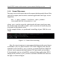
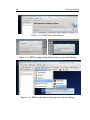
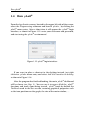
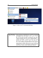
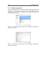
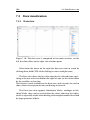
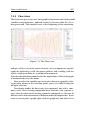
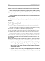
1
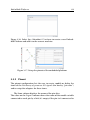
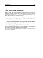
User’s Manual
for µLab 3
revision 1.0
2
Contents
1 Getting Started
1.1 Register on the web site and activate your muLab account
1.2 Installing an ssh client (putty) and setting the remote connection . . . . . . . . . . . . . . . . . . . . . . . . . . . . . .
1.2.1 Linux/Mac users . . . . . . . . . . . . . . . . . . . .
1.3 Install VNC viewer and connect to your remote desktop
session . . . . . . . . . . . . . . . . . . . . . . . . . . . . . .
1.3.1 Linux/Mac users . . . . . . . . . . . . . . . . . . . .
1.4 Run µLab® . . . . . . . . . . . . . . . . . . . . . . . . . . .
1.5 Copying your files into your µLab® remote account space
1.5.1 Linux/Mac users . . . . . . . . . . . . . . . . . . . .
1.6 Final touches . . . . . . . . . . . . . . . . . . . . . . . . . .
1.6.1 Change password . . . . . . . . . . . . . . . . . . . .
1.6.2 Change desktop resolution . . . . . . . . . . . . . .
1.7 MPLAB-X® issues . . . . . . . . . . . . . . . . . . . . . . .
1.7.1 MPLAB-X IDE® project setup . . . . . . . . . . . .
1.7.2 Error: Cannot start communication server . . . . .
1.7.3 Warning: muLab-MPLABX plugin detected that[...]
.
1
3
.
.
4
8
.
.
.
.
.
.
.
.
.
.
.
.
9
13
15
17
20
21
21
23
24
24
25
26
2 Interface Overview
27
2.1 The menu bar . . . . . . . . . . . . . . . . . . . . . . . . . . . 29
2.1.1 File menu . . . . . . . . . . . . . . . . . . . . . . . . . 29
2.1.2 Machine menu . . . . . . . . . . . . . . . . . . . . . . 31
Contents
4
2.1.3 Debug procedures menu . . .
2.1.4 Test sequences menu . . . . . .
2.1.5 Simulation menu . . . . . . . .
2.1.6 Help menu . . . . . . . . . . . .
The Tool bar . . . . . . . . . . . . . . .
The Tool bar for the Machine View . .
Test bench buttons . . .
Machine buttons . . . .
Zoom bar . . . . . . . . .
The Tool bar for the Simulation View
Simulation buttons . . .
The main pane . . . . . . . . . . . . .
2.5.1 Machine view . . . . . . . . . .
Graph pane . . . . . . .
Info pane . . . . . . . . .
2.5.2 Project Dictionaries view . . .
2.5.3 Debug Procedures view . . . .
2.5.4 Test Sequences view . . . . . .
2.5.5 Simulations view . . . . . . . .
The status bar . . . . . . . . . . . . . .
2.6.1 Log Console . . . . . . . . . . .
2.6.2 Status Info . . . . . . . . . . . .
2.6.3 Memory Usage icon . . . . . .
Notes and Reports . . . . . . . . . . .
2.7.1 Test Reports . . . . . . . . . . .
2.7.2 Working Notes . . . . . . . . . .
.
.
.
.
.
.
.
.
.
.
.
.
.
.
.
.
.
.
.
.
.
.
.
.
.
.
.
.
.
.
.
.
.
.
.
.
.
.
.
.
.
.
.
.
.
.
.
.
.
.
.
.
.
.
.
.
.
.
.
.
.
.
.
.
.
.
.
.
.
.
.
.
.
.
.
.
.
.
.
.
.
.
.
.
.
.
.
.
.
.
.
.
.
.
.
.
.
.
.
.
.
.
.
.
.
.
.
.
.
.
.
.
.
.
.
.
.
.
.
.
.
.
.
.
.
.
.
.
.
.
.
.
.
.
.
.
.
.
.
.
.
.
.
.
.
.
.
.
.
.
.
.
.
.
.
.
.
.
.
.
.
.
.
.
.
.
.
.
.
.
.
.
.
.
.
.
.
.
.
.
.
.
.
.
.
.
.
.
.
.
.
.
.
.
.
.
.
.
.
.
.
.
.
.
.
.
.
.
.
.
.
.
.
.
.
.
.
.
.
.
.
.
.
.
.
.
.
.
.
.
.
.
.
.
.
.
.
.
.
.
.
.
.
.
.
.
.
.
.
.
.
.
.
.
.
.
.
.
.
.
.
.
.
.
.
.
.
.
.
.
.
.
.
.
.
.
.
.
.
.
.
.
.
.
.
.
.
.
.
.
.
.
.
.
.
.
.
.
.
.
.
.
.
.
.
.
.
.
.
.
.
.
.
.
.
.
.
.
.
.
.
.
.
.
.
.
.
.
.
.
.
.
.
.
.
.
.
.
33
34
35
36
37
37
37
37
37
38
38
39
39
40
41
45
46
47
47
49
49
49
50
51
51
52
3 Machine/Process Modelling
3.1 Test bench . . . . . . . . . . . . . . . .
3.1.1 Creating a new test bench . . .
3.1.2 Loading an existing test bench
3.2 Components . . . . . . . . . . . . . . .
3.2.1 Component creation . . . . . .
3.2.2 Model type . . . . . . . . . . . .
3.2.3 Numerical model . . . . . . . .
.
.
.
.
.
.
.
.
.
.
.
.
.
.
.
.
.
.
.
.
.
.
.
.
.
.
.
.
.
.
.
.
.
.
.
.
.
.
.
.
.
.
.
.
.
.
.
.
.
.
.
.
.
.
.
.
.
.
.
.
.
.
.
.
.
.
.
.
.
.
.
.
.
.
.
.
.
.
.
.
.
.
.
.
.
.
.
.
.
.
.
53
53
53
54
55
55
55
56
2.2
2.3
2.4
2.5
2.6
2.7
Contents
5
3.2.3.1 Default Python model template . . . . . . .
3.2.3.2 Constant Gain model template . . . . . . . .
3.2.3.3 LaTeX model template . . . . . . . . . . . . .
3.2.3.4 Thermometer model template . . . . . . . .
3.2.3.5 Voltage Divider model template . . . . . . .
3.2.3.6 Wave Generator model template . . . . . . .
3.2.4 Parameters and variables . . . . . . . . . . . . . . . .
3.2.5 Pins and plugs . . . . . . . . . . . . . . . . . . . . . . .
3.2.6 Post-creation editing . . . . . . . . . . . . . . . . . . .
3.3 Embedded Platforms . . . . . . . . . . . . . . . . . . . . . . .
3.3.1 Embedded Platform creation . . . . . . . . . . . . . .
3.3.2 Pinout . . . . . . . . . . . . . . . . . . . . . . . . . . .
3.3.2.1 Clock frequency . . . . . . . . . . . . . . . .
3.3.2.2 Input voltage . . . . . . . . . . . . . . . . . .
3.3.2.3 Input/Output frequency-modulated pulse
train . . . . . . . . . . . . . . . . . . . . . . .
3.3.2.4 Input/Output width-modulated pulse train
3.3.2.5 Input/Output bit stream . . . . . . . . . . .
3.3.2.6 Device pin . . . . . . . . . . . . . . . . . . . .
3.3.3 Plugs . . . . . . . . . . . . . . . . . . . . . . . . . . . .
3.3.4 Post-creation editing . . . . . . . . . . . . . . . . . . .
3.4 Links . . . . . . . . . . . . . . . . . . . . . . . . . . . . . . . .
3.5 Groups . . . . . . . . . . . . . . . . . . . . . . . . . . . . . . .
4 Project Dictionaries Design
4.1 Dictionary of firmware variables/subroutines . . . . . . .
4.2 Dictionary of processor I/O signals . . . . . . . . . . . . .
4.3 Dictionary of processor implementations . . . . . . . . . .
4.4 Dictionary of runtime firmware subroutines substitutions
4.5 Dictionary of firmware implementations . . . . . . . . . .
4.6 Dictionary of external data files . . . . . . . . . . . . . . . .
4.7 Dictionary of post-process scripts . . . . . . . . . . . . . .
.
.
.
.
.
.
.
57
57
58
59
59
60
60
61
62
62
62
63
64
64
64
64
65
65
65
65
65
68
71
72
72
73
74
76
77
77
Contents
6
5 Debug Procedures Design
5.1 Creating a Debug Procedure . . . . . . . . . . . .
5.2 Renaming a Debug Procedure . . . . . . . . . .
5.3 Deleting a Debug Procedure . . . . . . . . . . . .
5.4 Creating/Editing/Deleting a Debug Instruction
5.5 Rearranging the Debug Instruction list . . . . .
.
.
.
.
.
.
.
.
.
.
.
.
.
.
.
.
.
.
.
.
.
.
.
.
.
.
.
.
.
.
.
.
.
.
.
83
83
83
84
85
87
6 Test Sequences Design
6.1 Creating a new Test Sequence . . . . .
6.2 Renaming a Test Sequence . . . . . .
6.3 Deleting a test sequence . . . . . . . .
6.4 Copy/Paste a test sequence . . . . . .
6.5 Creating/Editing/Deleting a new Test
6.6 Rearranging the Test list . . . . . . . .
.
.
.
.
.
.
.
.
.
.
.
.
.
.
.
.
.
.
.
.
.
.
.
.
.
.
.
.
.
.
.
.
.
.
.
.
.
.
.
.
.
.
.
.
.
.
.
.
.
.
.
.
.
.
.
.
.
.
.
.
.
.
.
.
.
.
.
.
.
.
.
.
.
.
.
.
.
.
89
89
89
90
90
91
91
7 Co-Simulations run
7.1 Starting Simulation . . . . . . .
7.1.1 Test selection . . . . . .
7.1.2 Machine configuration .
7.1.3 Links configuration . . .
7.1.4 Debug components . .
7.2 Simulation flow . . . . . . . . .
7.2.1 Pausing Simulations . .
7.2.2 Resuming Simulations .
7.2.3 Aborting Simulations . .
7.3 Data visualization . . . . . . . .
7.3.1 Data view . . . . . . . .
7.3.2 Chart view . . . . . . . .
7.3.3 Animation view . . . . .
7.3.4 Debug view . . . . . . .
7.4 Co-simulation logs . . . . . . .
7.5 Post Processing . . . . . . . . .
7.6 Test Reports . . . . . . . . . . .
7.6.1 Reports Manager . . . .
7.6.2 Text search tools . . . .
.
.
.
.
.
.
.
.
.
.
.
.
.
.
.
.
.
.
.
.
.
.
.
.
.
.
.
.
.
.
.
.
.
.
.
.
.
.
.
.
.
.
.
.
.
.
.
.
.
.
.
.
.
.
.
.
.
.
.
.
.
.
.
.
.
.
.
.
.
.
.
.
.
.
.
.
.
.
.
.
.
.
.
.
.
.
.
.
.
.
.
.
.
.
.
.
.
.
.
.
.
.
.
.
.
.
.
.
.
.
.
.
.
.
.
.
.
.
.
.
.
.
.
.
.
.
.
.
.
.
.
.
.
.
.
.
.
.
.
.
.
.
.
.
.
.
.
.
.
.
.
.
.
.
.
.
.
.
.
.
.
.
.
.
.
.
.
.
.
.
.
.
.
.
.
.
.
.
.
.
.
.
.
.
.
.
.
.
.
.
.
.
.
.
.
.
.
.
.
.
.
.
.
.
.
.
.
.
.
.
.
.
.
.
.
.
.
.
.
.
.
.
.
.
.
.
.
.
.
.
.
.
.
.
.
.
.
.
.
.
.
.
.
.
.
.
.
99
100
100
101
103
104
105
105
105
105
106
106
107
108
109
111
112
113
113
114
.
.
.
.
.
.
.
.
.
.
.
.
.
.
.
.
.
.
.
.
.
.
.
.
.
.
.
.
.
.
.
.
.
.
.
.
.
.
.
.
.
.
.
.
.
.
.
.
.
.
.
.
.
.
.
.
.
.
.
.
.
.
.
.
.
.
.
.
.
.
.
.
.
.
.
.
Contents
7
7.6.3 Report Groups management . . . . . . . . . . . . . . 115
7.7 Working Notes . . . . . . . . . . . . . . . . . . . . . . . . . . . 116
8
Contents
Chapter 1
Getting Started
This chapter describes the preliminary steps you should perform to start
using µLab® .
µLab® is meant to be executed as a cloud application, providing the
following advantages for its end-users:
• since all the heavy work is being performed in the cloud server,
the only system requirement we demand from the developer perspective is a reasonable internet connection; actually, a common
standard connection is sufficient to smoothly interact with µLab®
;
• because of this, you don’t need to update any of your computer
hardware;
• furthermore, because all of your projects run in a cloud server,
you can access and work on them from any locations and devices;
• multiple access are allowed, to give to a distributed teamwork the
possibility to interact within the same simulation.
Let us describe all the steps needed to get µLab® up and running, as
well to provide safety and security to all the data transitioning from your
2
Getting Started
computer/tablet to the server and viceversa. The current version of
this manual assumes by default that you are using the Windows operating system on your client computer, but the same operations can
be mad also with other other systems (Linux, Mac), as explained in the
Linux/Mac users subsection of each section.
Register on the web site and activate your muLab account
3
1.1 Register on the web site and activate your
muLab account
TO DO: UNDER CONSTRUCTION ...
Getting Started
4
1.2 Installing an ssh client (putty) and setting
the remote connection
As mentioned before, data security and safety are of primary concern.
Therefore, all communications between your local machine and the server
hosting µLab® should take place through an encrypted SSH connection.
To set up the connection, you first need to download and configure
PuTTY, freely available here.
Place a shortcut to it in a convenient place, such as in the desktop or
taskbar, then launch it. The first option to configure inside PuTTY is the
hostname to connect. From the Category sidebar, select Session subcategory; then, locate the label "Hostname (or IP address)" and, in the text
field immediately below it, enter the hostname mulab.simnumerica.com
.
A screenshot of this step is shown in Figure 1.1.
Figure 1.1: Hostname configuration
Installing an ssh client (putty) and setting the remote connection
5
Please ignore for now the Session entries: we will come back later.
Now, you need to supply your login credentials to PuTTY, so that it can
forward them to the cloud server. To perform this simple operation, just
head to the Connection -> Data subcategory, and locate the Auto-login
username label. On its right, instead of your_username shown in Figure 1.2 as example, insert the username you registered in the µLab®
registration page.
Figure 1.2: Username configuration
At this point, we are almost done with PuTTY configuration: it knows
to which server he has to connect, and which username present to it.
What it is still missing, is to define how to convey the remote desktop
session in the SSH secure channel. In other words, we have to define
now a tunnel connection.
To do so, head to the Connection -> Data -> SSH -> Tunnel subcategory,
and locate the Source port and Destination input boxes. Recalling the
port_number you got when you received the activation email response
(cfr. sec. 1.1), insert the port_number in the Source port and, as Des-
Getting Started
6
tination, insert localhost:port_number. See example in Figure 1.3,
with port_number equal to 5906.
Click Add to create a tunnelled connection, and you are done. Now, to
Figure 1.3: Tunnel configuration
save your time for every future connection, you can store this session
profile and load it when you need it. To do so, head back to Session
category, below the Saved Sessions label type a sensible name for that
connection ( in Figure 1.1 we saved it as muLab ), and then click Save.
Installing an ssh client (putty) and setting the remote connection
7
Now you can test your connection: double click on your earlier saved
session and a popup will show up, asking to trust our server. You just
need to answer Yes once: in subsequent connection attempts, that popup
will not show again.
Figure 1.4: Server trust request
Once you trusted our server RSA key, the command prompt will show
up. Enter your password, the one you choose when you registered in
the µLab® registration page, and you will see a command line prompt
pointing at your home directory, located inside the cloud server. See
Figure 1.5 as reference.
The command line is not the direct interface you will use in your working session. But, it activates the secure, tunnelled connection that VNC
will use to display the remote desktop, which is the interface you will
use to interact with µLab® (see sec. 1.3).
Getting Started
8
Figure 1.5: Successful connection to the remote server
1.2.1 Linux/Mac users
TO DO: UNDER CONSTRUCTION ...
Install VNC viewer and connect to your remote desktop session
9
1.3 Install VNC viewer and connect to your remote desktop session
Now you need to setup the application that will allow you to show the
remote desktop and work on it as if you were sitting in front of the cloud
server.
For this operation, you have to install TightVNC, freely available here.
Download and install it as you would do with any other application,
just remember not to install TightVNC Server because you only need its
client application to connet to our server. Therefore, choose the Cus-
Figure 1.6: TightVNC installation
tom installation mode as shown in the figure above, and then click on
the TightVNC Server entry and choose the option Entire feature will be
unavailable.
At this point, with the PuTTY command line still active, run the TightVNC
Viewer application: its interface is really minimal, you only have to specify the remote host and your specific port number, and then hit Connect
Getting Started
10
Figure 1.7: TightVNC installation
as shown in Figure 1.8 .
B Warning:
PuTTY connection must be running during the
whole VNC session. If you closed it, either accidentally or on purpose, you will lose your remote desktop connection
If everything was setup correctly, now you will be presented a messagebox asking for your password to login into your remote desktop environment.
Enter your password, and you are done! Welcome to your remote
desktop environment: you can start using µLab® .
Install VNC viewer and connect to your remote desktop session
Figure 1.8: VNC configuration
Figure 1.9: VNC authentication
11
Getting Started
12
Figure 1.10: VNC remote desktop
For a better view, you can expand the window to fit your screen ...
the µLab® GUI is designed for a full-screen usage.
If you wish, you can also set your VNC client to run in fullscreen mode.
In case of TightVNC, the shortcut to toggle fullscreen mode on and off is
CTRL+SHIFT+ALT+F.
B Warning:
If you think you may forget that shortcut combination, especially after a long session development,
you are encouraged to write it down. This is because you won’t be able to switch to another application (e.g. to read the PDF of this manual) until
you exit the fullscreen mode.
Install VNC viewer and connect to your remote desktop session
13
1.3.1 Linux/Mac users
To setup a successful connection to the remote desktop under Linux/Mac,
you have to open your favourite terminal application and type, in one
single line:
ssh -L <port_number>:localhost:<port_number>
<username>@mulab.simnumerica.com
where <port_number> must be substituted with your actual port number (the one you received by email) , and <username> of course by your
username in the remote server.
In the example below, we performed tunnelling of port 5909 for user
Diego
Figure 1.11: Linux/Mac tunneling
Now, the steps to connect to your remote desktop are the same shown
in Windows: just use your favourite VNC client shipped with your distribution, insert localhost:<port_number> as remote local host and click
Connect: once you provide your remote VNC password, you are done.
If, for example, you are using KDE’s remote desktop application KRDC,
simply insert localhost:<port_number> and then click the blue arrow on
the right, as shown in figure
Getting Started
14
Figure 1.12: KRDC host speficifation
Figure 1.13: KRDC config dialog, followed by the password dialog
Figure 1.14: KRDC with remote desktop active on user Diego
Run µLab®
15
1.4 Run µLab®
From the Applications menu, located in the upper left side of the screen,
select the Programming submenu and launch µLab® , by clicking the
µLab® menu entry. After a short time it will appear the µLab® login
interface, as shown in Figure 1.15: enter your username and password,
and start using the µLab® environment!
Figure 1.15: µLab® login interface
If you want to place a shortcut in the desktop instead, just right
click over µLab® menu entry and select Add this launcher to desktop,
as shown in Figure 1.16.
After the program has finished loading, the main µLab® dashboard
will be shown (see Cap. 2). You can use it to access all of the µLab®
functions and tools; upon being started, µLab® loads by default the
TestBench used in the last session, restoring graphical properties such
as the icon positions on the graph, the size of the main window, . . .
Getting Started
16
Figure 1.16: Run µLab® in the remote desktop
B Warning:
Once you have completed your µLab® session, do
not logout from your login in the server. If you
do so, you won’t be able to reconnect with your
remote desktop until the server administrator reactivate your login. Instead, just close VNC and
PuTTY: once you re-connect again, you will access
the same working environment left at the end of
your previous session (this can be very useful: for
example, if you left a simulation running, you will
access to its current status and interact with it).
Copying your files into your µLab® remote account space
17
1.5 Copying your files into your µLab® remote
account space
You have seen how to setup a secure connection, how to display your remote desktop session, and how to launch mulab. The natural step that
follows is to start composing one or more TestBench, i.e. your virtual
prototyping projects within µLab® : this requires also providing custom firmwares and some Python scripts (to model the physical world
interacting with your controller, to perform some postprocess actions,
etc.) that may have been written within another computer system.
In principle, you could develop everything from within your remote desktop session but, what your are most likely going to need, is a way to
transfer TestBench files and simulation datafiles from and to your remote account space. Thus, you need to download and install WinSCP
from here (free application).
Its interface is simple and intuitive, as well its setup: once you started it,
click on New button located in the upper rigth side of the application,
and the interface will change to let you enter details about the session
you are going to establish, as you can see in the image below
You only need to fill the following fields:
• Host name with mulab.simnumerica.com ;
• User name with your_username ;
• Password with your_password, the same used with PuTTY (cfr.
sec. 1.2);
After doing so, you can either press the Login button or, and we advise
you to do so, save this new session and then double click it from the
Stored sessions list.
If you did type everything correctly, after the connection phase you
will see a new window similar to the one shown in Figure 1.18: on the
left, you have your local directories and files; on the right, you can explore your remote account directory and subfolders. If you want to upload a file or folder from your local computer to the server, just drag and
Getting Started
18
Figure 1.17: WinSCP setup page
Figure 1.18: WinSCP connected to mulab remote account space
drop it from the left panel to the right panel. In Figure 1.19 for example,
we copied the local folder mulab inside
C:\mulab\modules\branches into the remote folder /root/Downloads. Win-
Copying your files into your µLab® remote account space
19
SCP is smart enough to provide some transfer options to better improve
the transfer rate and reduce bandwidth usage: feel free to try them and
then press the Copy button.
Figure 1.19: WinSCP folder upload to remote server
Getting Started
20
1.5.1 Linux/Mac users
If you are running any GNU/Linux distribution, you can copy any file
and folder with the handy scp command. It takes the following parameters:
• the file or folder you need to transfer (when transferring folders,
remember to add the -r parameter to send the folder and its content, recursively);
• the username in the cloud server, hostname, and destination folder
(absolute path) where the file/folder will be placed.
An example of transfer operation of folder firmware (empty in that case),
executed by user Diego, into his own remote Desktop folder, is show in
the figure below: The first time you perform this operation, scp will ask
Figure 1.20: Folder transfer operation using scp command
you if you are sure to connect with the host: just reply yes, and the server
credentials will be saved for the future connections.
TO DO: UNDER CONSTRUCTION ...
Final touches
21
1.6 Final touches
Now that you are able to setup a secure connection to the cloud server,copy
files and folders into it, and start µLab® , there are some final touches
you are likely interested to perform as well.
1.6.1 Change password
For example, you may want to change your login password and your
VNC password to something different than the ones you received from
the administrator email. This process is really fast and easy to perform,
so we highly encourage you to do so.
To change your user login password, open a new terminal and type
the passwd command, as shown in Figure 1.21.
Figure 1.21: Login password change
The prompt will ask for your current password and then it will ask
Getting Started
22
you to enter your new password twice. If everything went good, the
prompt will inform you that your authentication tokens were updated
successfully.
An almost identical process applies if you change VNC password, as you
can see in Figure 1.22.
Figure 1.22: VNC password change
In fact, now you have to type the command vncpasswd and, as opposed to passwd, it will not ask for your current vnc password but it will
simply ask for a new one to set.
Final touches
23
1.6.2 Change desktop resolution
Another aspect you most likely want to change is the desktop resolution.
It is a really straightforward operation if you already used Gnome desktop environment. If you never did, just follow the screenshot in Figure
1.23.
Figure 1.23: Change desktop resolution
Getting Started
24
1.7
MPLAB-X® issues
There are a few issues that an MPLAB-X® user must keep in mind, when
doing co-simulations with µLab® .
1.7.1
MPLAB-X IDE® project setup
In order to perform a successful co-simulation session, you need to properly set up your MPLAB-X IDE® project as we will immediately show.
First, your project must be compiled with the new toolchains provided by Microchip along with MPLAB-X IDE® 1 that is, XC8/16/32
compilers.
B Warning:
if you import an older project that has been developed with MPLAB IDE v8 or previous versions, remember to change the compiler from mpasm or
C18/30 one of its new counterpart, otherwise the
plugin will misbehave and the co-simulation will
not take place.
In addition to the compiler, you also need to choose the right Hardware Tool for the project you want to test. In fact, µLab® needs to query
MPLAB-X IDE® internal simulator about the register and pinout states;
therefore, you have to choose the Simulator option as current Hardware
Tool. You can find both compiler and hardware tool options by right
clicking the corresponding project listed in the Project panel. An example dialog is shown in figure 1.24.
The last detail you need to take care of is setting the right frequency for
the simulator.
1 See http://www.microchip.com/pagehandler/en-us/family/mplabx , Compilers section
MPLAB-X® issues
25
Figure 1.24: Project options
B Warning:
setting the clock frequency in µLab® will not have
any effect on MPLAB-X® simulator, so please remember to do it from within MPLAB-X IDE® .
1.7.2 Error: Cannot start communication server
This error arises for the following three reasons:
• the plugin was not installed, or it was removed because you
wanted to upgrade it, but then you forgot to install the newer
version;
Solution ⇒ contact the administrator
• there is an instance of MPLAB-X IDE® already running, and
µLab® cannot connect to it because it has to start MPLAB-X
IDE® on its own
Solution ⇒ save everything you were working in MPLAB-X
IDE® and close it: µLab® will start it and take
26
Getting Started
care of its startup and communication setup
1.7.3 Warning: muLab-MPLABX plugin detected that[...]
When you see a warning message which tells you “muLab-MPLABX plugin detected that the frequency in the simulator is different from the one
set by the Clock Frequency Adapter”, it means that you are trying to run
a simulation but the frequency you set on OSC1/OSC2 is different from
the one used from MPLAB-X IDE® internal simulation and, therefore,
you will get erroneus results. To solve this issue, update the correct oscillator frequency value in the MPLAB-X® project, or change the frequency parameter of the AdapterClockFrequency attached to OSC1/OSC2
(see sec. 3.3.2.1).
Chapter 2
Interface Overview
The main µLab® dashboard is composed of 4 sections:
• the Menu Bar;
• the Toolbar;
• the Main Pane;
• the Status Bar;
and includes a WYSIWYG text editor for writing notes (and examining
test reports, see 2.18) during your µLab® work session.
This chapter explains how to navigate the dashboard and access all
of the main µLab® functionalities; you can find specific details in the
corresponding sections.
28
Interface Overview
Figure 2.1: The main µLab® dashboard
The menu bar
29
2.1 The menu bar
The menu bar contains several menus used to manage the contents of
your machine and your tests.
2.1.1 File menu
Figure 2.2: The File menu
The File menu (figure 2.2) is used to manage your test bench files.
New test bench: create a new, empty test bench. See also 3.1.1 for a
detailed walkthrough.
Load test bench: load an existing test bench from a test bench file. See
also 3.1.2 for a detailed walkthrough.
Save test bench: save the current test bench to file. This is only active if
the test bench has been modified after the last save.
Rename test bench: rename the current test bench. Renaming requires
the test bench to be saved (you will be asked for confirm).
About current test bench: show a brief description of the test bench
you are currently working on.
30
Interface Overview
Quit: terminate all of the active simulations and debug procedures and
exit µLab® .
The menu bar
31
2.1.2 Machine menu
Figure 2.3: The Machine menu
The Machine menu (figure 2.3) lets the user define the hardware
setup of the machine, by creating the components themselves and their
interconnections, that model their interactions. The resulting machine
can be viewed by selecting the Machine icon from the navigation bar.
New component: create a new component and add it to your machine.
See also 3.2.1 for detailed instructions about creating components.
New embedded platform: create a new embedded platform and add it
to your machine. See also 3.3.1 for detailed instructions about creating embedded platforms.
New link: setup a connection between two existing items. See also 3.4
for detailed instructions about links.
Edit: edit the properties of the selected item.
Remove: remove the selected item from your machine.
Group: create a group containing the selected items. See also 3.5 for
more instructions about groups.
32
Interface Overview
Ungroup: remove the selected group relation between items, without
removing the items from the machine. See also 3.5 for more instructions about groups.
The menu bar
33
2.1.3 Debug procedures menu
Figure 2.4: The Debug Procedures menu
The debug procedures menu (figure 2.4) lets you create, edit and remove debug procedures. For more info about debug procedures, see
Chapter 5.
New debug procedure: start the creation of a new debug procedure. See
also 5.1.
Edit debug procedure: modify the properties of an existing debug procedure. See also 5.4 for editing individual debug instructions.
Remove debug procedure: delete the selected debug procedure. See
also 5.3.
Interface Overview
34
2.1.4 Test sequences menu
Figure 2.5: The Test Sequences menu
The test sequences menu (figure 2.5) lets you create, edit and remove test sequences. For more info about test sequences, see Chapter
6.
New test sequence: start the creation of a new test sequence. See also
6.1.
Edit test sequence: modify the properties of an existing test sequence.
See also 6.5 for editing individual tests.
Remove test sequence: delete the selected test sequence. See also 6.3.
The menu bar
35
2.1.5 Simulation menu
Figure 2.6: The Simulation menu
The Simulation menu (figure 2.6) lets you start numerical simulations on your machine, control the flow of their execution, and access
the simulation docs. For more info about simulations, see also Chapter
7.
Start simulation: start the Simulation launch wizard. See also 7.1 for
detailed instructions about launching simulations and test sequences.
Pause: pause the current simulation; inactive if no simulations are running. See also 7.2.1.
Resume: resume the current simulation; inactive if no simulations are
active and paused. See also 7.2.2.
Cancel: abort the current simulation; inactive if no simulations are active. See also 7.2.3.
Docs: open the workbench notes and test reports managers.
Interface Overview
36
2.1.6 Help menu
Figure 2.7: The Help menu
The Help menu (figure 2.7) lets you access various assistance tools.
Online Help: open the integrated µLab® Online Help. TO DO: S EE
?? FOR MORE INFO AND SUGGESTIONS ON HOW TO USE IT EFFEC TIVELY.
Java system properties: open a viewer that lists the Java properties of
your system. Cannot be used to modify their values.
OS environment variables: open a viewer that lists the environment
variables of your system. Cannot be used to modify their values.
About: show an informative popup about µLab® .
The Tool bar
37
2.2 The Tool bar
The Tool bar provides quick shortcuts for the most commonly used functions of the Menu bar. It changes with the view selected in the Navigation Bar, as described in the following sections.
2.3 The Tool bar for the Machine View
Figure 2.8: The Tool bar
Test bench buttons
• new test bench;
• load test bench.
Machine buttons
• new component;
• new embedded platform;
• new link;
• edit item;
• remove item.
Zoom bar
You can use this scroll bar to select the zoom level for the graph.
Move the slider to the left to zoom out, and move it to the right to zoom
in.
Interface Overview
38
2.4 The Tool bar for the Simulation View
Simulation buttons
• start simulation;
• debug simulation;
• pause current simulation;
• resume current simulation;
• abort current simulation;
• open simulation docs.
The main pane
39
2.5 The main pane
Use the Navigation Bar to choose between the Machine view, the Project
Dictionaries view, the Debug Procedures view, the Test Sequences view,
and the Simulation view for the main pane.
2.5.1 Machine view
Figure 2.9: The Machine view
The Machine view is used to show and edit the machine you’re currently working on.
This view is split in two main panes: the left one is used to work on the
machine structure, while the right one can be used to set up masks, view
and edit variables and parameters of the model, and modify the look of
the graph.
40
Interface Overview
Figure 2.10: Machine view, the Graph pane
Graph pane The machine itself is represented by a graph; the nodes of
the graph represent the components of the machine, and the arcs of the
graph represent the links of the machine.
Component and link properties can be modified through the respective edit dialogs, accessible by double clicking the object you want to
edit (or by selecting it and then choosing the Edit action from the Machine menu or the toolbar).
Components and links can be deleted through the Delete action,
which can be selected from the Machine menu, the toolbar, or the context menu (open it by right-clicking on the component). Del (on your
The main pane
41
keyboard) also works as a generic shortcut for deletion.
Figure 2.11: Machine view, the Info pane
Info pane TO DO: TROVARE NOME DECENTE PER LA SEZIONE;
The right section of the machine view consists of the Info pane. It is a
panel whose contents depend on the current graph selection. TO DO:
DA METTERE IN FORMA DI TABELLA
• No items selected
Model view: shows machine masks, machine details, parameters
(all), variables (all).
– Machine masks: lets you choose and setup machine masks;
– Machine details: ID, name, description of the machine;
– Parameters: a name, value pair list of all of the parameters in the machine components;
Interface Overview
42
– Variables: a name [type], initial value pair list of all of
the variables in the machine components.
Graph view: shows graph properties.
– Grid visible: toggle this to show a grid underneath the
graph (disabled by default);
– Grid aspect: the way the underlying graph grid is drawn
(crosses, dots, lines);
– Grid color: the color of the grid;
– Grid size: the size of the grid elements;
– Background color: the background color of the graph.
• One component selected
Model view: shows component details, parameters, variables, plugs
and pins.
– Component details: ID, name, description, model file,
enabled (if this option is toggled off, the status of the
component will not change during simulations TO DO:
CHE SIGNIFICA ?;
– Parameters: a name, value pair list of the component
parameters;
– Variables: a name [type], initial value pair list of the component variables;
– Plugs and pins: a list containing the component plugs;
each plug is composed of two name [type], initial value
pairs describing its pins.
Graph view: shows vertex properties.
– ID: the component ID;
– Font: the font used for the component name in the graph;
– Icon: the icon used to represent the component in the
graph;
– Background color: the background color for the component square in the graph;
The main pane
43
– Foreground color: the foreground color for the component square in the graph;
– Bounds: the bounds of the component square in the
graph;
– Border visible: if toggled on, shows the border of the
component square in the graph.
• One embedded platform selected
Model view: shows embedded platform details, plugs and pins,
processors.
– Embedded platform details: ID, name, description, enabled (if this option is toggled off, the status of the embedded platform will not change during simulations TO
DO: CHE SIGNIFICA ?;
– Plugs and pins: a list containing the embedded platform
plugs; each plug is composed of two name [type], initial
value pairs describing its pins.
– Processors: a list containing the embedded platform microprocessors; each processor entry shows a list containing all of its pins.
Graph view: shows vertex properties.
– ID: the embedded platform ID;
– Font: the font used for the embedded platform name in
the graph;
– Icon: the icon used to represent the embedded platform
in the graph;
– Background color: the background color for the embedded platform square in the graph;
– Foreground color: the foreground color for the embedded platform square in the graph;
– Bounds: the bounds of the embedded platform square
in the graph;
Interface Overview
44
– Border visible: if toggled on, shows the border of the
embedded platform square in the graph.
• One link selected
Model view: shows link details, connections, wires.
– Link details: ID, name, description, enabled (if this option is toggled off, the status of the link will not change
during simulations TO DO: CHE SIGNIFICA ?;
– Connections: two plug type, name pairs describing (source
and target) plugs connected by this link;
– Wire: a list of pin [type], initial value pair couples describing the pins (and the initial values of the variables
they carry) connected by the wires of this link.
Graph view: shows edge properties.
– ID: the link ID;
– Font: the font used for the link name in the graph;
– Line style: the line style for this link (bezier, orthogonal,
spline);
– Line begin: the style for the beginning of this link line
(none, circle, simple, technical, classic, diamond, line,
double line);
– Line end: the style for the ending of this link line (none,
circle, simple, technical, classic, diamond, line, double
line);
– Line color: the color of this link line in the graph;
– Line width: the width of this link line in the graph.
• More than one item selected
Model view: no properties to show.
Graph view: no properties to show.
• Groups
Nothing happens by clicking on groups.
The main pane
45
2.5.2 Project Dictionaries view
The Project Dictionaries view lets you manage the dictionaries of all the
relevant project items defined in the current TestBench. Each panel,
from left to right and from top to bottom, containes the following dictionaries:
• the Dictionary of firmware variables/subroutines, cfr sec. 4.1;
• the Dictionary of processor I/O signals, cfr. sec. 4.2;
• the Dictionary of processor implementations, cfr. sec. 4.3;
• the Dictionary of external data files, cfr. sec. 4.6;
• the Dictionary of runtime firmware subroutines substitutions, cfr.
sec. 4.4;
• the Dictionary of firmware implementations, cfr. sec. 4.5;
• the Dictionary of post-process scripts, cfr. sec. 4.7.
Figure 2.12: The Project Dictionaries view
Interface Overview
46
Figure 2.13: The Debug Procedures view
2.5.3 Debug Procedures view
The Debug Procedures view lets you manage the debug procedures for
the current test bench.
The list on the left pane displays the available debug procedures:
you can click the New Debug Procedure button at the bottom to create
a new one, or click an existing one to show the instructions it is composed of, and use the buttons at the bottom to rename or delete it.
The debug instructions editor works in a similar way: click the New
Debug Instruction button to add a new debug instruction at the end of
the debug procedures, or click an existing one and then use the buttons
at the bottom of the pane to edit its contents or delete it.
More info about designing Debug Procedures can be found in Chapter
5 and in the µLab® Tutorial.
Please note that debug instructions are executed in a sequential order, but every new instruction is added at the bottom of the list: you can
use the arrow buttons on the right to change the position of the selected
debug instruction.
The main pane
47
2.5.4 Test Sequences view
Figure 2.14: The Test Sequences view
The Test Sequences view lets you manage the test sequences for the
current test bench.
The list on the left pane displays the available test sequences: you
can click the New Test Sequence button at the bottom to create a new
one, or click an existing one to show the single tests it is composed of,
and use the buttons at the bottom to rename or delete it.
The tests editor works in a similar way: click the New Test button to
add a new test at the end of the sequence, or click an existing one and
then use the buttons at the bottom of the pane to edit its contents or
delete it.
More info about designing Test Sequences can be found in Chapter 6
and in the µLab® Tutorial.
2.5.5 Simulations view
The Simulations view lets you watch real-time data evolution during the
execution of a test sequence.
See Chapter 7 for detailed info about simulation data.
Interface Overview
48
Figure 2.15: The Simulations view
The status bar
49
2.6 The status bar
The Status Bar is shown in Figure 2.16 and contatins, from left to right,
the Log Console, the Status Info, the Memory Usage icon and the name
of the current TestBench.
Figure 2.16: The Status bar
2.6.1 Log Console
Figure 2.17: The Log console
Clicking the Show Log Console icon opens up a display area for errors, warnings and informative messages regarding the operations being performed in µLab® . It is possible to copy part of the log console contents into the system clipboard by selecting the text you want to
copy, and then pressing ctrl-c or right clicking on the text display area
and selecting copy from the context menu. If no text is selected, the
entire contents of the log console are copied.
2.6.2 Status Info
Any relevant status messages are shown here.
50
Interface Overview
2.6.3 Memory Usage icon
This bar shows how much memory is being used by the Java Virtual Machine.
Double clicking the Virtual Machine memory usage icon explicitly
calls the Java Garbage Collector.
Notes and Reports
51
2.7 Notes and Reports
You can open the Simulation Docs dialog through the Simulation menu.
This dialog lets you access the Notes and Reports panels.
2.7.1 Test Reports
You can specify annotations to be recorded during the execution of any
debug instruction through the Debug Instruction Editor. As soon as the
simulation is over, µLab® saves these lines in a test report: such files
can be accessed and managed through the Report Manager.
See sec. 7.6 for more details about Test Reports.
Figure 2.18: The Reports manager
Interface Overview
52
2.7.2 Working Notes
µLab® features an integrated rich text editor for taking notes within the
application.
Working notes belong to the test bench they are saved in: as such, when
a test bench folder is moved to another µLab® installation, its working
notes are carried over to the new copy (on the other hand, you can only
access a working note from the testbench it belongs to).
Figure 2.19: The Notes manager
The list on the left shows the available notes for the active test bench.
Click the New button to create a new note, adding it to the list and opening it in the editor, or double-click an existing list entry (alternatively,
select it and press the Load button) to open the corresponding note for
editing.
See sec. 7.7 for more details about Test Reports.
Chapter 3
Machine/Process Modelling
3.1 Test bench
A test bench is composed of the machine model, the debug procedures
and test sequences, the firmware projects and the python substitutions,
the external data files, the post-processing scripts, the working notes
and the test reports.
This set of objects is stored in the files inside the test bench directory:
creating (or loading) a test bench basically means creating (or loading)
such a set.
3.1.1 Creating a new test bench
To create a test bench, select New test bench from the File menu. A
pop-up window appears (Figure 3.1) where you will be asked to indicate
the name, the author, the image icon and the location on your hard drive
of the new test bench you want to create. Once the above information
is provided, you can click the Create tab and generate the test bench.
54
Machine/Process Modelling
Figure 3.1: Fill in the test bench creation form to continue
3.1.2 Loading an existing test bench
To load an existing test bench, select Load test bench from the File
menu, and select the test bench you want to load through the file chooser
dialog (test bench directories can be distinguished from their red “µ"
icon). The selected test bench will be loaded onto the working environ-
Figure 3.2: Select a test bench and press Load to continue
ment.
Components
55
3.2 Components
3.2.1 Component creation
In order to add a new component to the machine model, select Add
component from the Machine menu, or press the button shown in Figure 3.3, to open the Component creation wizard (Figure 3.4). The first
Figure 3.3: Press the New component button to create a new component
and add it to the current machine
page of the wizard allows you to specify the name (required) and add a
brief description (optional) of the new component; then press Next.
Figure 3.4: Name and description of the new component
3.2.2 Model type
Now, choose an available model type and then press Next. In this release of the software we consider only the Python model type.
Machine/Process Modelling
56
Figure 3.5: Model type of the new component
3.2.3 Numerical model
The following step of the wizard requires you to formulate the numerical
model of the new component.
Once you’ve decided the model type, you may have to specify some
additional settings. This operation is strongly dependent from the model
type you selected. For the Python model type, cfr. Figure 3.6, click the
New python model button and choose one of the existing implementation templates, cfr. Figure 3.7.
Figure 3.6: Python component solver setup
Components
Figure 3.7:
chooser
57
Python component solver implementation templates
3.2.3.1 Default Python model template
This template is an empty Python model with only the interface with
the µLab® model. Write the implementation of this model between the
code lines
# <YOUR CODE (START)>: put here the actual solution of the component model.
and
# <YOUR CODE (END)> .
When you have done, click the Generate button. At this point, see
Figure 3.8, the Python code is ready to be checked (by pressing the Check syntax
button), to eventually run its test routine (by pressing the Run module
button) if you decided to code it, and to save it in a file named <component name>.py.
If the code verification process, after pressing the Check syntax
button, succeeds, you will see the pop-up of Figure 3.9; otherwise, you
will see the pop-up of Figure 3.10.
Analogously, if the run of the test routine, after pressing the Run module
button, succeeds, you will see the pop-up of Figure 3.11.
3.2.3.2 Constant Gain model template
TO DO: DESCRIPTION ...
Machine/Process Modelling
58
Figure 3.8: Python component solver code verification
Figure 3.9: Python component solver code verification success
3.2.3.3 LaTeX model template
Thanks to the CfL Link , µLab® can generate Python component models from a text written in LaTeX. Supposing you have a file latex with
the component model equations written according to the CfL® standard, this template lets you upload the file latex from the chooser of
Figure 3.12. Press the “...” button and choose your latex file, as shown
in Figure 3.13 for the file example_Lorentz.tex, then press Open. Now
click the Generate button. Wait the end of the code generation process,
Components
Figure 3.10: Python component solver code verification failure
Figure 3.11: Python component solver test routine run success
which will produce a success pop-up as in Figure 3.9.
3.2.3.4 Thermometer model template
TO DO: DESCRIPTION ...
3.2.3.5 Voltage Divider model template
TO DO: DESCRIPTION ...
59
Machine/Process Modelling
60
Figure 3.12: LaTeX component solver setup
Figure 3.13: LaTeX component solver file chooser
3.2.3.6 Wave Generator model template
TO DO: DESCRIPTION ...
3.2.4 Parameters and variables
The third step of the wizard lets you set up parameters and variables of
your new component.
Within each component, parameters and variables are uniquely identified by their name.
Components
61
µLab® lets you use the same name for a parameter and a variable in the
same component, or for more than one parameter (or variable) as long
as each of them belongs to a different component; however, preserving
name uniqueness (when possible) always remains a good practice.
You may also add a mnemonic symbol and a brief description.
To complete the setup of a parameter you have to provide its value
(defaults to zero) and its unit of measurement (defaults to adimensional).
Likewise, to complete the setup of a variable you have to provide its type
(Input, Output or State), its initial value (defaults to zero), its unit of
measurement (defaults to adimensional) and its resolution, as shown
in Figure 3.14. If the component model has been created from a LaTeX
Figure 3.14: Model parameters and variables
file (see sec. 3.2.3.3), also its parameters and variables are automatically
created and you will find them in the tables of Figure 3.14.
3.2.5 Pins and plugs
The fourth step of the wizard lets you add plugs to your component.
Click on the New icon to create a new plug, then specify its name and
pins: each pin can be associated to an I/O variable (the type of the pin
Machine/Process Modelling
62
Figure 3.15: Click the New plug button to create a plug
is the same of the variable); you can add multiple pins to a plug, and
multiple plugs to a component.
3.2.6 Post-creation editing
You may also modify the newly added component after the wizard has
been completed: to open the editor, either double click the component
icon on the graph, or select it and click the Edit item in the Machine
menu.
3.3 Embedded Platforms
3.3.1 Embedded Platform creation
To add a new Embedded Platform, select New embedded platform from
the Machine menu. This opens up the wizard of Figure 3.16: input the
name (required) and a brief description (optional) of the new embedded platform, then press Next to continue.
Embedded Platforms
63
Figure 3.16: Select New Embedded Platform to create a new Embedded Platform and add it to the current machine
Figure 3.17: Setup the pinout of the embedded platform
3.3.2 Pinout
The pinout configuration lets the user to create, modify or delete the
items of the Dictionary of processor I/O signals (for brevity, “pin alias”)
and to setup the adapters for these items.
The Name column displays the name of the pin alias.
The value on the Signal column shows the name of the model variable
connected to each pin by a link (it’s empty if the pin isn’t connected to
64
Machine/Process Modelling
any components).
The Adapter column lets you specify (and then configure) adapters for
each pin alias: click on the description of the adapter (it’s empty if no
adapters have been configured for that pin alias) to edit it. Each adapter
type is described in the following subsections.
3.3.2.1 Clock frequency
Here the user can set the external clock frequency input to the microcontroller. The adapter accepts one parameter Clock frequency [Hz]
and no connections are required to the pin of the embedded platform
model (eventual data fed up to the pin are not considered).
3.3.2.2 Input voltage
Here the user can set a constant input voltage, with no need to build
an external component in the µLab® model. The adapter accepts one
parameter Constant voltage [V] and no connections are required
to the pin of the embedded platform model (eventual data fed up to the
pin are not considered).
3.3.2.3 Input/Output frequency-modulated pulse train
Here the user can generate/read a high frequency-modulated pulse train
at microcontroller pins, without the need to sample the µLab® model
at the Nyquist frequency of the signal or higher. The adapter accepts
one parameter Duty cycle [%] and reads/writes the value at the embedded platform pin as the frequency of the pulse train.
3.3.2.4 Input/Output width-modulated pulse train
Here the user can generate/read a high frequency width-modulated pulse
train at microcontroller pins, without the need to sample the µLab®
model at the Nyquist frequency of the signal or higher. The adapter accepts one parameter Frequency [Hz] and reads/writes the value at the
embedded platform pin as the duty cycle of the pulse train.
Links
65
3.3.2.5 Input/Output bit stream
Here the user can generate/read a serial bit stream at microcontroller
pins, without the need to sample the µLab® model at the Nyquist frequency of the signal or higher. The adapter accepts two parameters,
Baud rate and Message length and reads/writes the values at the
embedded platform pin as the bit stream.
3.3.2.6 Device pin
TO DO: ...
3.3.3 Plugs
The final step of the wizard lets you add plugs to your embedded platform.
Click on the New icon to create a new plug, then specify its name and
pins: each pin can be associated to an I/O variable (the type of the pin
is the same of the variable); you can add multiple pins to a plug, and
multiple plugs to an embedded platform. After all the plugs have been
created, press Ok to end the embedded platform creation wizard.
3.3.4 Post-creation editing
You may also modify the newly added embedded platform after the wizard has been completed: to open the editor, either double click the embedded platform icon on the graph, or select it and click the Edit item
in the Machine menu.
3.4 Links
In order to create a working machine, its components must be linked to
each other; you can do this by creating links from the Machine menu
(Machine → New link) or with the button shown in Figure 3.19.
66
Machine/Process Modelling
Figure 3.18: Plug configuration dialog: specify the name of the plug and
the pins it’s composed of.
Figure 3.19: Select New link to start the link creation wizard
Doing so brings up the link creation wizard (Fifure 3.20). Input the
name (required) and a brief description (optional) of the new link, then
press Next to continue.
Connections between two components of any machine are formed
by linking one plug on each machine with each other, as shown in Figure
3.21.
Such a connection can only be made if the two plugs are compatible.
Compatibility between plugs is verified by checking if all of the pins on
the first plug can be correctly connected with all of the pins on the second plug.
Two pins can be connected with each other if their I/O types are compatible (i.e. if the first is an input pin and the second is an output pin
or vice versa, or if one is a microp pin) and if their units of measure-
Links
67
Figure 3.20: The link creation wizard:specify the name of the new link;
you may add a description text (optional). When you are done, press
Next to continue.
Figure 3.21: Select source and target plugs of the new link.
ment are the same. Note that the connection begins at the output pin
and ends at the input pin.
Different numbers of pins, or failure to match one or more pins on
one plug, will cause the two plugs to be incompatible, therefore unavailable for being connected with each other.
Machine/Process Modelling
68
Figure 3.22: The selected plugs are compatible: drag the output/microp
pins to the input/microp pins to create wires. Press Finish when done.
Figure 3.23: The selected plugs are not compatible for connection
3.5 Groups
Selecting multiple components (by either clicking them one by one while
pressing ctrl or shift, or by doing a rectangle selection) enables the group
Groups
69
command on the toolbar
Figure 3.24: Drag a box around the components you want to group. You
may now press the Group button to group them
Upon creating a group, you’ll be asked for a group name (cannot be
blank).
Figure 3.25: Specify the name of the new group and press OK to create it
A group can be either collapsed (only the group icon and name are
shown on the graph, its contents hidden) or expanded (no group icon
and name, all of its contents are shown): you can switch between the
two display modes by clicking on the expand/collapse button on the top
left corner. It’s possible to change the contents of a group without destroying and recreating it: expand it, and drag the component you want
to add (or remove, respectively) inside (or outside) the group box. If you
want to remove a group, select it and press the ungroup button. Note
that this only deletes the group view, not the components themselves.
70
Machine/Process Modelling
Figure 3.26: Collapsed and expanded views of a group. Press + to switch
between the two modes
Figure 3.27: Components being added to (left picture) and removed
from (right picture) a group through drag-and-drop
Figure 3.28: Ungrouping removes the old group relationship between
objects, but the components themselves are not deleted
Chapter 4
Project Dictionaries Design
72
Project Dictionaries Design
4.1 Dictionary of firmware variables/subroutines
In order to create, modify or delete an alias of a firmware variable/subroutine,
use the panel and the buttons indicated in Figure 4.1.
Figure 4.1: Here it is the list of firmware variable/subroutine aliases;
at the left bottom there are four buttons to create a variable (”blue
star”), create a subroutine (”yellow star”), modify the selected variable/subroutine (”pencil”), delete the selected variable/subroutine
(”thrash”); then, press OK to actuate the selected action or cancel to
abandon it.
4.2 Dictionary of processor I/O signals
In order to create, modify or delete an alias of a processor I/O signal (for
brevity, “pin alias”), see sec. 3.3.2.
Dictionary of processor implementations
73
4.3 Dictionary of processor implementations
In order to create, modify or delete a processor implementation, use
the panel and the buttons indicated in Figure 4.2. The editor is shown
in Figure 4.3.
Figure 4.2: Here it is the list of processor implementations existing in
the project; at the left bottom there are three buttons to create, modify
or delete the selected implementation.
Figure 4.3: The editor of a processor implementation: the user should
specify a name, and the bindings with the simulator, the specific device
inside the simulator and the alias-physical pins association.
Project Dictionaries Design
74
4.4 Dictionary of runtime firmware subroutines
substitutions
The dictionary of runtime firmware subroutines substitutions (see an
example in Figure 4.4), is located in the left bottom of the Project Dictionaries View (sec. 2.5.2).
Figure 4.4: An example of a dictionary of runtime firmware subroutines
substitutions
In order to:
• create a new substitution, press the leftmost button (a new item
appears, as a blue table row), then click on the cells from the left
to choose:
– the alias of the firmware function to be substituted, see Fig.
4.5;
– the arguments that could be passed to this firmware subroutine (Fig. 4.6); possible arguments are: items of the Dictionary of firmware variables (sec. 4.1), items of the Dictionary of the processors I/O signals and model parameters (sec.
3.2.4);
– the python module containing the function that substitutes
the firmware subroutine (4.7) and the python function itself
(by writing its name in the text field).
Dictionary of runtime firmware subroutines substitutions
75
• create a substitution from a LaTeX file, press the second button
from left, and then submit the file selected through a standard file
chooser;
• edit the python module, select a substitution (table row) and press
the third button from the left;
• delete a substitution, press the the rightmost button (thrash icon).
Figure 4.5: Select the alias of the firmware function to be substituted,
and press Choose to confirm the selection or cancel to discard it.
76
Project Dictionaries Design
Figure 4.6: Choose the arguments by typing them (Ctrl+Space does
the auto-completion) and press the circle buttons to add or delete an
argument from the list; press OK to confirm the selection list or cancel
to discard it.
Figure 4.7: Select the python file with the standard chooser of the OS.
4.5 Dictionary of firmware implementations
In order to create, modify or delete a firmware implementation, use the
panel and the buttons indicated in Figure 4.8. The editor of a firmware
implementation is shown in Figure 4.9 and the editor of a firmware variable/subroutine binding is shown in Figure 4.10.
Dictionary of external data files
77
Figure 4.8: Here it is the list of firmware implementations existing in the
project; at the left bottom there are three buttons to create, modify or
delete the selected implementation.
4.6 Dictionary of external data files
In order to create, modify or delete a reference to an external datafile,
use the panel and the buttons indicated in Figure 4.11. The editor is
shown in Figure 4.14.
4.7 Dictionary of post-process scripts
In order to create, modify or delete a postprocessing script, use the panel
and the buttons indicated in Figure 4.13. The editor is shown in Figure
4.14.
78
Project Dictionaries Design
Figure 4.9: The editor of a firmware implementation: the user should
specify a name, the project dir, he must press the Load firmware symbols button, choose the compiler and the processor implementation
and the bindings with the variables and the subroutines implemented
in the firmware project and corresponding to the dictionary items.
Dictionary of post-process scripts
79
Figure 4.10: The editor of a firmware variable/subroutine binding: the
user double click the alias of a variable/subroutine and the editor open
up. He then must choose the Name of the variable corresponding to
the selected alias, among the symbols defined in the firmware project
and presented in a popup list of the editor; he must also specify the
Type of the variable/subroutine-return-value and, if the variable is a C
struct/vector, the offset in bytes at which the desired scalar value is allocated.
Figure 4.11: Here it is the list of references to external datafiles considered in the project; at the left bottom there are three buttons to create,
modify or delete the selected implementation.
80
Project Dictionaries Design
Figure 4.12: The editor of a reference to an external datafile: the user
should specify a name, the datafiles involved in this reference (usually
there is a single datafile), and the bindings of each column of data with
the corresponding project item, that can be: items of the Dictionary of
firmware variables (sec. 4.1), items of the Dictionary of the processors
I/O signals and model parameters and variables (sec. 3.2.4).
Figure 4.13: Here it is the list of the postprocessing scripts existing in
the project; at the left bottom there are three buttons to create, modify
or delete the selected implementation.
Dictionary of post-process scripts
81
Figure 4.14: The editor of a postprocessing script: the user should specify a name, the python file containing the postprocessing script, and
write the python code of the script.
82
Project Dictionaries Design
Chapter 5
Debug Procedures Design
Use the navigation bar from the main µLab® dashboard to access the
Debug Procedures View (sec. 2.5.3): it allows the user to design the Debug Procedures to be used in the project. Its structure is shown in Figure
5.1:
5.1 Creating a Debug Procedure
From the Debug Procedures page, click the Create new debug procedure button; then input the name of the new debug procedure and
press OK to continue.
5.2 Renaming a Debug Procedure
To rename a debug procedure, select it from the list and click the Edit
procedure button.
84
Debug Procedures Design
Figure 5.1: The Debug Procedures View: there are two vertical sections,
that show the list of the existing Debug Procedures (left) and the list of
the Debug Instructions (right) existing in the selected Debug Procedure.
5.3 Deleting a Debug Procedure
To delete a debug procedure, select it and click the Remove procedure
button.
Creating/Editing/Deleting a Debug Instruction
85
Figure 5.2: Input a name for the new Debug Procedure and press OK to
continue
5.4 Creating/Editing/Deleting a Debug Instruction
Click the Create new Debug Instruction button to start the creation
of a new Debug Instruction that will be added at the bottom of the instructions list of the current Debug Procedure. To edit a debug instruction, select it from the list and press the Edit instruction button. To
remove a debug instruction from the debug procedure, select it from the
list and press the Remove instruction button. To change the position
of a Debug Instruction inside a Debug Procedure, use the arrow buttons
as shown in Figure 5.6. The Debug Instruction editor is shown in Figure
5.5.
Configure the new Debug Instruction through the Debug Instruction Editor (refer to the µLab® tutorial for detailed information on how
86
Debug Procedures Design
Figure 5.3: Select a Debug Procedure and click Edit Procedure to rename it
to configure debug instructions).
Rearranging the Debug Instruction list
87
Figure 5.4: Select a Debug Procedure and click Remove Procedure to
remove it from the list
5.5 Rearranging the Debug Instruction list
You can use the up and down buttons to move up or down (by one step)
a debug instruction.
Debug instruction fulfilling their activation and execution conditions
will be performed in this order.
88
Debug Procedures Design
Figure 5.5: Click Create new Debug Instruction to add a new Debug Instruction
Figure 5.6: Click the arrow buttons to move a Debug Instruction up or
down the list
Chapter 6
Test Sequences Design
Use the navigation bar from the main µLab® dashboard to access the
Test Sequences View (sec. 2.5.4): it allows the user to create and delete
Test Sequences, and edit their contents. Its structure is shown in Figure
6.1:
6.1 Creating a new Test Sequence
From the Test Sequences page, click the Create new test sequence
button; input the name of the new test sequence and press OK to continue.
6.2 Renaming a Test Sequence
To rename a test sequence, select it from the list and click the Edit
test sequence button.
90
Test Sequences Design
Figure 6.1: The Test Sequences View: there are two vertical sections, that
show the list of the existing Test Sequences (left) and the list of the Tests
(right) defined in the selected Test Sequence.
6.3 Deleting a test sequence
To delete a test sequence, select it and click the Remove test sequence
button.
6.4 Copy/Paste a test sequence
To copy/paste a test sequence, select it and click first the Copy test
sequence button; then select the position to paste a copy of the Test
Sequence and click the Paste test sequence button (Figure 6.5).
Creating/Editing/Deleting a new Test
91
Figure 6.2: Input a name for the new Test Sequence and press OK to continue.
6.5 Creating/Editing/Deleting a new Test
Click the Create new Test button to start the creation of a new Test
that will be added at the bottom of the current Test Sequence. To edit a
test, select it from the list and press the Edit test button. To remove a
test from the test sequence, select it from the list and press the Remove
test button. The Test editor has multiple tabs:
• Details, , is shown in Figure 6.6;
• Details, , is shown in Figure 6.7;
• Details, , is shown in Figure 6.8;
• Details, , is shown in Figure 6.9;
• Details, , is shown in Figure 6.10;
6.6 Rearranging the Test list
You can use the up and down buttons to move up or down (by one step)
a test (Figure 6.11).
92
Test Sequences Design
Figure 6.3: Select a Test Sequence and click Edit test sequence to
rename it.
When a test sequence is started with the Launch all tests option
active, tests are performed in the same order they are found in the sequence, even though they are independent (i.e. machine states don’t
carry over between subsequent tests).
Rearranging the Test list
93
Figure 6.4: Select a Test Sequence and click Remove test sequence to
delete it.
94
Test Sequences Design
Figure 6.5: Select a Test Sequence and click Copy test sequence and
Paste test sequence (rightmost buttons).
Rearranging the Test list
95
Figure 6.6: Click.
Figure 6.7: Click.
96
Test Sequences Design
Figure 6.8: Click Create new Test to add a new Test in the Test Sequence.
Figure 6.9: Click Create new Test to add a new Test in the Test Sequence.
Rearranging the Test list
97
Figure 6.10: Click Create new Test to add a new Test in the Test Sequence.
Figure 6.11: Click the arrow buttons to move a Test up or down the list
98
Test Sequences Design
Chapter 7
Co-Simulations run
Use the navigation bar from the main µLab® dashboard to access the
Simulation View (sec. 2.5.5): it allows the user to monitor the running
Tests interactively, and to do some post-processing. Its structure is populated only when there is at least one Test running or finished, and it is
shown in Figure 7.1:
Figure 7.1: The Test Simulation View :
Co-Simulations run
100
7.1 Starting Simulation
In order to launch a Simulation, you have to perform a few basic steps,
described in the following subsections.
7.1.1 Test selection
There are two ways to select a Test or a Test Sequence:
• From any view in µLab® : click the Launch Test or the Launch
Test Sequence buttons (Figure 7.2) to show the Test Sequence selection screen (Figure 7.3). Note that pressing the Launch Test Sequence button causes all of the contained Tests to be run one after
another, sequentially. Moreover, every test is unrelated from the
others (i.e. machine states don’t carry over between two consecutive tests).
Figure 7.2: The Launch Test (left) and the Launch Test Sequence (right)
buttons.
• From the Test Sequences View: if a Test Sequence and eventually
also a Test are selected in this view, click the Launch Test or the
Launch Test Sequence buttons; the selection made will bypass the
Test Sequence selection screen (Figure 7.3) and bypass also the
Test selection screen (Figure 7.4), if also a Test is selected in this
view or the Launch Test Sequence button has been pressed.
Starting Simulation
101
Figure 7.3: Choose a test sequence from the list and click Next
Figure 7.4: Select the test you want to execute and click Next
7.1.2 Machine configuration
Machine variables and parameters are displayed in a tree-structured table, grouped by component (and by processor model in case they belong to an embedded platform); any values specified here will override
both the starting default values (only for the execution of the selected
102
Co-Simulations run
Test or Test Sequence) and the values in the specific Test configurations.
Figure 7.5: Configure the starting values of variables and parameters
Starting Simulation
103
7.1.3 Links configuration
Each link between model components can be here enabled or disabled;
any values specified here will override both the starting default values
(only for the execution of the selected Test or Test Sequence) and the
values in the specific Test configurations.
Figure 7.6: Configure the starting values of variables and parameters
104
Co-Simulations run
7.1.4 Debug components
Select which components you want to debug during the execution of the
simulation (select multiple components by pressing CTRL while clicking them). Note that only the components that support debugging will
be available for selection.
Figure 7.7: Select the components you want to debug by clicking them
while pressing CTRL.
Figure 7.8: Select the components you want to debug by clicking them
while pressing CTRL.
Simulation flow
105
7.2 Simulation flow
The simulation flow can be controlled with the buttons shown in Figure
7.2.
Figure 7.9: The flow control buttons, from left to right: Pause, Resume
and Cancel
7.2.1 Pausing Simulations
Use this command to pause the execution of the Test shown in the active
tab.
7.2.2 Resuming Simulations
Use this command to resume the execution of the Test shown in the
active tab.
This action can only be performed if the Test was previously paused: an
aborted Test cannot be resumed.
7.2.3 Aborting Simulations
Use this command to stop and abort the execution of the current Test.
Aborting a Test also cancels the creation of its Test Reports.
106
Co-Simulations run
7.3 Data visualization
7.3.1 Data view
Figure 7.10: The data view is composed of two main sections: on the
left, the data tables; on the right, the selection panes
Select from the menu on the right the data you want to watch by
clicking them; hold CTRL while clicking to select multiple items.
The Data view shows the last value taken by the selected items; specifying an instant in the text field on the right lets you see the values taken
by the variables at that time.
This feature is only available in the data view, and can only be used to
show values at one given instant, not during an interval.
The Data view also supports Simulation Masks: analogue to Machine Masks, they can be used to filter the values shown in the tables,
which is especially useful when dealing with complex models described
by large quantities of data.
Data visualization
107
7.3.2 Chart view
The chart view gives you a real-time graphical representation of the model
variables and parameters, updated instant by instant while the Test is
being executed. The timeline starts at the beginning of the simulation,
Figure 7.11: The Chart view
and goes all the way to the current instant: you can zoom on a specific
region by indicating it with the mouse pointer, and scrolling with the
wheel (scroll up to zoom in, scroll down to zoom out).
Note that the minimum zoom level is the original one; click on the graph
to automatically reset the zoom.
You can select the variables you want to be shown in a graph by clicking on their names in the selection panel: press ctrl while clicking for
multiple selection.
Two display modes for data series are supported: one with a common y-axis, when viewing comparable data, and one with separate yaxes, when the data you’re viewing cannot be compared (i.e. because of
different units of measurement or different orders of magnitude). If you
want to save or print a graph, right-click the graph area and select Save
Co-Simulations run
108
Figure 7.12: Common and separate y-axis modes buttons
or Print from the context menu.
7.3.3 Animation view
This functionality is forthcoming.
This view lets you use the simulation data as input variables for a
graphical animation. Custom animations can be added to the built-in
set: write the Java FX script that implements your animation, opportunely binding its variables to the simulation parameters, and place the
script file in the test bench folder.
Data visualization
109
7.3.4 Debug view
The debug view lets you modify breakpoints and watch variables, parameters and memories while the simulation is running. Click on a line
Figure 7.13: The Debug view
number/instruction address to add a breakpoint on that line; click again
to remove it. When the execution of the platform firmware or component solver stops at a breakpoint (Figure 7.14), you can use the control
buttons to either skip that breakpoint, do one step (that is, execute the
current instruction and stop at the next one), or continue the simulation
(until the following breakpoint is reached), see Figure 7.15.
Click the Memories button to show a watch table for variables data
(Figure 7.16).
Co-Simulations run
110
Figure 7.14:
simulation
Active breakpoints in the embedded firmware co-
Figure 7.15: Debug control buttons
Figure 7.16: Click the Memories button to watch variables
Co-simulation logs
7.4 Co-simulation logs
TO DO: ...
111
Co-Simulations run
112
7.5 Post Processing
TO DO: ...
Figure 7.17: The Post Processing simulation view:
Test Reports
113
7.6 Test Reports
Test Reports are automatically created during the execution of Simulations.
Open the Simulation Docs window and click the Test Reports tab
to access the Reports Manager.
Figure 7.18: Docs simulation view: the Test Reports tab
7.6.1 Reports Manager
The layout of the Reports Manager is composed of two parts:
• on the left, the list of the Test Reports stored in the active testbench;
• on the right, the Test Report editor.
Reports can be opened in the editor by double-clicking their name
on the list;
Co-Simulations run
114
groups instead can be expanded or collapsed by double-clicking them.
Right-clicking the tab of a Report in the editor shows a pop-up menu
you can use to close that report, close all of the other reports, or close all
of the open reports.
Select a Report on the list and click the Delete button to delete the
selected Report.
Click the Search Reports button to open the advanced search tools
window.
7.6.2 Text search tools
The µLab® Reports Manager provides you with two text search tools.
You may search for a string in the currently active Report by using
the Search text field at the bottom of the Report panel.
Any text matching the specified string will be then highlighted in the active Report, and the editor will scroll to show the first match instance.
If you need to search for a string in all of the Reports stored in the
active testbench, without opening every single one of them in the editor, open the advanced search tools window by clicking the Search Reports button.
Specify the string you want to search in the Search text field, select
one of the two result display modes, and click Ok to perform the search:
• search reports and show list looks for matches with the specified string and displays a list of the Reports containing any matches;
you may then pick which Reports to open by selecting them on
the list (press CTRL while clicking them for multiple selections)
and clicking Choose;
• search reports and open them looks for matches with the specified string and automatically open all of the Reports containing
Test Reports
115
any matches.
7.6.3 Report Groups management
Report Groups are created by default when you execute a whole Test
Sequence; a Report generated by the execution of a single Test (that is,
by using the Launch just 1 test in the sequence setting), by default, does not belong to any Report Groups.
Double click on a Group to expand or collapse it: expanding a Group
shows a list of the Reports it contains.
Select a set of Reports (press CTRL while clicking the single Reports
for multiple selection) and click the Create button to create a new group
containing the selected Reports;
select an existing group and click Rename to rename it;
select an existing group and click Dissolve to remove the Group only:
the Reports it contained will become single Reports;
select an existing group and click Delete to remove the Group and delete
the Reports it contains.
Co-Simulations run
116
7.7 Working Notes
Working Notes are automatically created during the execution of Simulations.
Open the Simulation Docs window and click the Working Notes tab.
Figure 7.19: Docs simulation view: the Working Notes tab