Download r8s, version 1.50 User`s Manual

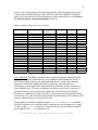
1
r8s, version 1.50
User’s Manual
(August 2002)
Michael J. Sanderson
Section of Evolution and Ecology, One Shields Avenue,
University of California, Davis, CA 95616, USA
email:[email protected]
Introduction
This is a program for estimating absolute rates (“r8s”) of molecular evolution and
divergence times on a phylogenetic tree. It implements several methods for estimating
these parameters ranging from fairly standard maximum likelihood methods in the
context of global or local molecular clocks to more experimental semiparametric and
nonparametric methods that relax the stringency of the clock assumption using smoothing
methods. Its starting point is a given phylogenetic tree and a given set of estimated
branch lengths (numbers of substitutions along each branch). In addition one or more
calibration points can be added to permit scaling of rates and times to real units. These
calibrations can take one of two forms: assignment of a fixed age to a node, or
enforcement of a minimum or maximum age constraint on a node, which is generally a
better reflection of the information content of fossil evidence. Terminal nodes are
permitted to occur at any point in time, allowing investigation of rate variation in
phylogenies such as those obtained from “serial” samples of viral lineages through time.
Finally, it is possible to assign all divergence times (perhaps based on outside estimates
of divergence times) and examine molecular rate variation under several models of
smoothing.
The motivation behind the development of this program is two-fold. First, the abundance
of molecular sequence data has renewed interest in estimating divergence times (e.g.,
Wray et al. 1996; Ayala et al. 1998; Kumar and Hedges 1998; Korber et al. 2000), but
there is wide appreciation that such data typically show strong departures from a
molecular clock. This has prompted considerable theoretical work aimed at developing
methods for estimating rate and time in the absence of a clock (Hasegawa et al. 1989;
Takezaki et al. 1995; Rambaut and Bromham 1998; Sanderson 1997; Thorne et al. 1998;
Hulesenbeck et al. 2000; Kishino et al. 2001). However, software tools for this are still
specialized and generally do not permit the addition of flexible calibration tools.
Second, there are surprisingly few estimates of absolute rates of molecular evolution
constructed in a phylogenetic framework. Most estimates are based on pairwise distance
2
methods with simple fixed calibration points (e.g., Wray et al. 1996; Kumar and Hedges
1998). This program is designed to facilitate estimation of rates of molecular evolution,
particularly estimation of the variability in such rates across a tree.
Powerful tools are available for phylogenetic analysis of molecular data, such as the
magnificent PAUP* 4.0 (Swofford 1999), but none of them is designed from the ground
up to deal with time. The default molecular models are generally atemporal in the sense
that they estimate branch lengths that consist of nondecomposable products of rate and
time. PAUP* and PAML and other programs can, of course, enforce a molecular clock
and reconstruct a tree in which the branch lengths are proportional to time, but the time of
the root of such a tree is arbitrary. It can be scaled manually a posteriori by the user given
the age of single fossil attached to a single node in the tree, but none of these programs
permit the addition of several calibration points or minimum or maximum age
constraints. Moreover, they do not consider models that are intermediate between the
clock on the hand and completely unconstrained rate variation on the other hand (the
default). This has proven extremely useful for tree-building but may be limited for the
purposes of understanding rate variation and estimating divergence times.
This program does not implement all or even most methods now available for estimating
divergence times. In particular, it does not implement highly parametric Bayesian
approaches described by Thorne et al. (1998, or the later Kishino et al. 2001) or
Huelsenbeck et al. (2000). It provides, as a benchmark, routines that implement a
molecular clock. It also includes methods for analyzing user-specified models with k
discrete rates (where k is small). These are particular useful for looking at correlates of
rate variation. For example, one might assign all lineages leading to species of annual
plants in a phylogeny one rate, and those leading to the perennial species a second rate.
However, the main thrust of the program is to implement methods that are nonparametric
or semiparametric rather than parametric per se. By analogy to smoothing methods in
regression analysis, these methods attempt to simultaneously estimate unknown
divergence times and smooth the rapidity of rate change along lineages. The latter is done
by invoking some function that penalizes rates that change too quickly from branch to
neighboring branch. The first, wholly nonparametric, method, nonparametric rate
smoothing (NPRS: Sanderson 1997) consists of essentially nothing but the penalty
function. Since the function includes unknown times, a suitably constructed optimality
criterion based on this penalty can permit estimation of the divergence times. This
method, however, tends to overfit the data leading to rapid fluctuations in rate in regions
of a tree that have short branches.
Penalized likelihood (Sanderson 2002) is a method that combines likelihood and the
nonparametric penalty function used in NPRS. It permits specification of the relative
contribution of the rate smoothing and the data-fitting parts of the estimation procedure.
The user can any level of smoothing from severe, which essentially leads to a molecular
clock to effectively unconstrained. A cross validation procedure is also provided to
provide a data-driven method for finding the optimal level of smoothing.
3
Installation
The program is currently available as a Linux binary for x86 machines. The binary
executable file together with several sample data sets are bundled together in a
compressed archive file. After downloading the file r8s.dist.tar.Z to your account,
uncompress and untar it with the following commands
uncompress r8s.dist.tar.Z
tar xvf r8s.dist.tar
This sets up a directory called dist which has four subdirectories, bin, sample, doc,
and src. The first has the executable, the second has several sample data files, the third
contains various versions of this manual and the fourth contains the source code.You may
want to move the executable file, r8s, into the path that your account uses to look for
binary files. If you have a system administrator, or you have root access yourself, you can
install the program in some place like /usr/local/bin so that everyone can have access
to it. If you have not set the PATH variable for your account and are frustrated that you
cannot get the program to execute, you may have to type ./r8s rather than just r8s,
assuming the program is in your current working directory.
You can check the version number of the program with the r8s –v switch.
If you wish to install the source code, a makefile is included that works on linux
machines. There are known incompatibilities with some other compiler's libraries or
headers, most of which are easy to resolve. You must own a copy of Numerical Recipes
in C (Press et al. 1992 or more recent versions) to compile and run from source.
Note to users of versions prior to 1.0
Many of the features and much of the syntax has changed since pre-release versions were
made available. Most important is the addition of the required blformat command,
which obviated the clunky convert_branchlength_to_time and
multiply_branchlength_by commands. The rates block is now (optionally) called the
r8s block. Several other command names or option names have been changed. Note that
the program generally just ignores a command it does not understand, rather than issuing
a warning. This can lend you a false sense of security. Examine the sample data files
carefully and read all the documentation before modifying your old files.
Changes since version 1.05
The most significant change is the addition of a new black box optimization routine to
carry out truncated Newton optimization with simple bound constraints. The code, called
TN, is due to Stephen Nash and is written in fortran. Further information is available at
NetLib (http://www.netlib.org), where the code is distributed. In general, this code is
much faster and better at finding correct solutions. However, it relies on gradients, which
4
I have still only derived for Langley-Fitch (clock) and Penalized Likelihood methods. It
is not yet implemented for NPRS.
A large number of bugs have been fixed, including some serious memory leaks. See the
revision history in the doc directory of the distribution.
Some definitions
A cladogram is a phylogenetic tree in which branch lengths have no meaning. A
phylogram is a tree in which branch lengths correspond to numbers of substitutions along
branches (or numbers of substitutions per site along that branch). A chronogram is a
phylogenetic tree in which branch lengths correspond to time durations along branches. A
ratogram is a tree in which branch lengths correspond to absolute rates of substitution
along branches (apologies for the jargon).
Running the program
The program can be run in batch or interactive modes. The default is interactive mode,
usually executed from the Linux (bash) prompt as follows:
r8s –f datafile <cr>
This invokes the program, reads the data file, containing a tree or trees and possibly some
r8s commands, and presents a prompt for further commands. Typing q or quit will exit
the program.
Batch mode is invoked similarly but with the addition of the –b switch:
r8s –b –f datafile <cr>
This will execute the commands in the data file and return to the operating system
prompt. Finally, note that the –f switch and datafile is optional. The program can be
run interactively with just
r8s <cr>
It is possible to subsequently load a data file from within r8s with the execute command
(see command reference).
The output from a run can be saved to a file using standard Linux commands, such as
r8s –b –f datafile > outfile
Notice that if you neglect to include the –b switch in this situation, the program will sit
there patiently waiting for keyboard input. You may think it has crashed...
5
Data file format
The program reads ASCII text files in the Nexus format (Maddison et al., 1997), a
standard that is being used by increasing numbers of phylogenetic programs (despite the
grumblings of Nixon et al. 2001). At a minimum the data file should have a Trees block
in it that contains at least one tree command (tree description statement). The tree
command contains a tree in parentheses notation, and optionally may include branch
length information, which is necessary for the divergence time methods described below.
Thus, the following is an example of a nearly minimal datafile named ‘Bob’ that r8s can
handle:
#nexus
begin trees;
tree bob = (a:12,(b:10,c:2):4);
end;
Upon execution of
r8s –f Bob <cr>
the program will come back with a prompt allowing operations using this tree.
It is usually easiest to imbed these r8s commands into a special block in the data file
itself and then run the program in batch mode. For example:
#nexus
begin trees;
tree bob = (a:12,(b:10,c:2):4);
end;
begin r8s;
blformat lengths=total nsites=100 ultrametric=no;
set smoothing=100;
divtime method=pl;
end;
followed by
r8s –f bob –b <cr>
The meaning of the commands inside the r8s block will be discussed below. All
commands described in this manual can be executed within the r8s block.
Grammar for r8s block and r8s commands
All r8s commands must be found within a r8s block:
6
begin r8s;
command1;
command2;
.
.
.
end;
All r8s commands follow a syntax similar to that used in PAUP* and several other
Nexus-compliant programs, which will be described used the following conventions:
command option1=value1|value2|… option2=value1|…
(etc);
Thus any command might have several options, each of which has several alternative
values. The vertical bars delimit alternative choices between values. Values may be
strings, integers, real numbers, depending on the option. Default values are underlined.
There are only a few exceptions to this general grammar.
Required information in the r8s block.
The program needs a few pieces of information about the trees and the format of the
branch lengths stored in the Trees block. This is provided in the blformat command,
which should be the first command in the r8s block. Its format is
blformat lengths=total|persite nsites=nnnn ultrametric=no|yes
round=no|yes;
The lengths option indicates the units used for branch lengths in the tree descriptions.
Depending on the program and analysis used to generate the branch lengths, the units of
those lengths may vary. For parsimony analyses, the units are typically total numbers of
substitutions along the branch, whereas for maximum likelihood analyses, they are
typically expected numbers per site, which is therefore dependent on sequence length.
The nsites option indicates how many sites are in the sequences that were used to
estimate the branch lengths in PAUP or some other program. Take care to insure this
number is correct in cases in which sites have been excluded in the calculations of branch
lengths (e.g., by excluding third positions in PAUP and then saving branch lengths). The
program does not recognize exclusion sets or other PAUP commands that might have
been used in getting the branch lengths.
The ultrametric option indicates whether the branch lengths were constructed using a
model of molecular evolution that assumes a molecular clock (forcing the tree and branch
lengths to be ultrametric). If ultrametric is set to yes then uncalibrated ages are
immediately available for the trees. To calibrate them against absolute age, issue a
calibrate command, which scales the times to the absolute age of one specific node in
the tree. This linear stretching or shrinking of the tree is the only freedom allowed on an
7
ultrametric tree. Multiple calibrations might force a violation of the information provided
by the ultrametric branch lengths. Do not use the fixage command on such trees unless
you wish to re-estimate ages completely.
The round option is included mainly for analyses of trees that are already ultrametric
rather than estimation of divergence times using the divtime command. Ordinarily input
branch lengths are converted to integer estimates of the number of substitutions on each
branch (by multiplying by the number of sites and rounding). This is done because the
likelihood calculations in divtime use numbers of substitutions as their data. However,
when merely calibrating trees that are already ultrametric, rounding can generate branch
lengths that are not truly ultrametric, because short branches will tend to be rounded
inconsistently. When working with ultrametric, user-supplied chronograms, set
round=no.
If the program is run in interactive mode, this blformat command should be executed
before any divergence time/rates analysis, although other commands will work without
this.
Naming nodes/clades/taxa
Many commands refer to internal nodes in the tree, and it is often useful to assign names
to these nodes. For example, it is possible to constrain the age of internal nodes to some
minimum or maximum value, and the command to do this must be able to find the correct
node. Every node is also the most recent common ancestor (“MRCA”) of a clade.
Throughout the manual an internal node may be referred to interchangeably as a “node
name” , “clade name”, or “taxon name.”
The program uses two methods to associate names with internal nodes. One is available
in the Nexus format for tree descriptions. The Nexus format permits internal nodes to be
named by adding that name to the appropriate right parenthesis in a tree description. For
example
tree betty=(a,(b,c)boop);
assigns the name boop to the node that is the most recent common ancestor of taxon b
and c.
This method is obviously error prone and not very dynamic. Therefore r8s has a special
command to permit naming of nodes. The command
MRCA boop a b;
will assign the name boop to the most recent common ancestor of a and b. The name of a
terminal taxon can also be changed by dropping one of the arguments:
8
MRCA boop a;
assigns the name boop to terminal taxon a.
Fixing and constraining times prior to estimating divergence times
One or more nodes can have its age fixed or constrained prior to estimating the
divergence times of all other nodes using the divtime command. Time is measured
backward from the most recent tip of the tree, which is assumed to have a time of 0 by
default. In other words, times might best be thought of as “ages” with respect to the
present. Note: the following commands are not appropriate if the input tree is already
ultrametric—use calibrate instead.
Fixed and free nodes. Any node in the tree, terminal or internal, can have its age fixed or
free. A node that is fixed has an age that is set to a specific value by the user. A node that
is free has an age that must be estimated by the program. By default, all internal nodes in
the tree are assumed to be free, and all terminal nodes are assumed to be fixed, but any
node can have its status changed by using the fixage or unfixage command. The format
for both of these commands is similar:
fixage taxon=angio age=150;
unfixage taxon=angio;
It is possible to fix all internal node ages with
fixage taxon=all;
or to unfix them all with
unfixage taxon=all;
but note that this applies (by default) only to internal nodes. To unfix the age of a
terminal taxon, you must specify each such taxon separately:
unfixage taxon=terminal1;
unfixage taxon=terminal2;
Fixing the age of nodes generally makes it easier to estimate other ages or rates in the
tree—that is it reduces computation time, because it reduces the number of parameters
that must be estimated. Roughly speaking, the divergence time algorithms require
that at least one internal node in the tree be fixed, or that several nodes be constrained
as described below. If this is awkward, it is always possible to fix the root (or some other
node) to have an arbitrary age of 1.0, and then all rates and times will be in units scaled
by that age. Under certain conditions and with certain methods, the age of unfixed nodes
cannot be estimated uniquely. See further discussion under “Uniqueness of solutions.”
9
Ages persist on a tree until changed by some command. Sometimes it is desirable
to retain an age for a particular node but to fix it so that it is no longer estimated in
subsequent analyses. This can be accomplished using fixage but not specifying an age:
fixage taxon=sometaxon;
Constrained nodes. Any node can also be constrained by either a minimum age or a
maximum age. This is very different from fixing a node’s age to a specific value, and it
only makes sense if the node is free to be estimated. Computationally it changes the
optimization problem into one with linear inequality constraints, which does not remove
any parameters, and is much more difficult solve anyway. The syntax for these
commands is given in the following examples:
constrain taxon=node1 min_age=100;
constrain taxon=node2 min_age=200 max_age=300;
and to remove constraints on a particular node:
constrain taxon=node1 min_age=none;
or to remove all such constraints across the entire tree (including terminals and internals):
constrain remove=all;
Once a constraint is imposed on a node, divergence time and rate algorithms act
accordingly. No further commands are necessary.
The words minage and maxage can be used instead of min_age, max_age.
Estimation of rates and times
The divtime command, with numerous options, provides an interface to all the
procedures for estimating divergence times and absolute rates of substitution. Given a
tree or set of trees with branch lengths, and one or more times provided with the fixage
or constrain commands, the divtime command provides calibrated divergence times
and absolute rates in substitutions per site per unit time.
The simplified format of the divtime command is
divtime method=LF|NPRS|PL algorithm=POWELL|TN|QNEWT;
The first option describes the method used; the second describes the type of numerical
algorithm used to accomplish the optimization.
10
Methods. The program currently implements four different methods for reconstructing
divergence times and absolute rates of substitution. The first two are variations on a
parametric molecular clock model; the other two are nonparametric or semiparametric
methods.
LF method. The Langley-Fitch method (Langley and Fitch, 1973, 1974) uses maximum
likelihood to reconstruct divergence times under the assumption of a molecular clock. It
estimates one substitution rate across the entire tree and a set of calibrated divergence
times for all unfixed nodes. The optimality criterion is the likelihood of the branch
lengths. A chi-squared test of rate constancy is reported. If a gamma distribution of rates
across sites is used, the appropriate modification of the expected Poisson distribution to a
negative-binomial is used (see under Theory below).
LF “local molecular clock” method. This relaxes the strict assumption of a constant rate
across the tree by permitting the user to specify up to k separate rate parameters. The user
must then indicate for every branch in the tree which of the parameters are associated
with it. This is useful for assigning different rates for different clades or for different
collections of branches that may be characterized by some biological feature (such as a
life history trait like generation time).
The first step in running this method is to “paint” the branches of the tree with the
different parameters. Assume that there will be k rate parameters, where k > 1. The
parameters are labeled as integers from 0,…, k-1. The default Langley-Fitch model
assigns the rate parameter “0” to every branch of the tree, meaning there is a single rate
of evolution. Suppose we wish to assign some clade “bob” a different rate, “1”. Use the
following command:
localmodel taxon=bob stem=yes rateindex=1;
The option stem=yes|no is necessary if the taxon refers to a clade. It indicates whether
the branch subtending the clade is also assigned rate parameter “1”. It is important to use
all integers from 0,…, k-1, if there are k rate parameters. The program does not check,
and estimates will be unpredictable if they do not match. Using this command it is
possible to specify quite complicated patterns of rate variation with relatively few
commands.
The local molecular clock procedure is then executed by
divtime method=lf nrates=k;
where k must be greater than 1. If k = 1, then a conventional LF run is executed. It is
important to remember that with this approach it is quite easy to specify a model that will
lead to degenerate solutions. To detect this, multiple starting points should always be
run (see below under search strategies). One robust case is when the two sister groups
descended from the root node have different rates.
11
NPRS method. Nonparametric rate smoothing (Sanderson, 1997) relaxes the assumption
of a molecular clock by using a least squares smoothing of local estimates of substitution
rates. It estimates divergence times for all unfixed nodes. The optimality criterion is a
sum of squared differences in local rate estimates compared from branch to neighboring
branch.
PL method. Penalized likelihood (Sanderson, 2002) is a semiparametric approach
somewhere between the previous two methods. It combines a parametric model having a
different substitution rate on every branch with a nonparametric roughness penalty which
costs the model more if rates change too quickly from branch to branch. The optimality
criterion is the log likelihood minus the roughness penalty. The relative contribution of
the two components is determined by a “smoothing parameter”. If the smoothing
parameter, smoothing, is large, the objective function will be dominated by the
roughness penalty. If it is small, the roughness penalty will not contribute much. If
smoothing is set to be large, then the model is reasonably clocklike; if it is small then
much rate variation is permitted. Optimal values of smoothing can be determined by a
cross-validation procedure described below.
Algorithms. The program uses three different numerical algorithms for finding optima of
the various objective functions. In theory, it should not matter which is used, but in
practice, of course, it does. The details of how these work will not be described here.
Eventually I hope to incorporate all algorithms in all the methods described above, but at
the moment only Powell’s algorithm is available for all methods. Table 1 indicates which
algorithms are available for which methods and under what restrictions. Unless you are
doing NPRS or the local clock model, I recommend the new TN algorithm.
Powell. Multidimensional optimization of the objective function is done using a
derivative-free version of Powell’s method (Gill et al. 1981; Press et al. 1992). This
algorithm is available for each of the three methods. However, it is not as fast, or as
reliable as quasi-newton methods (QNEWT), which require explicit calculations of
derivatives. For the LF algorithm, its performance is quick and effective at finding
optima; for NPRS and PL, it sometimes gets trapped in local optima or converges to flat
parts of the objective function surface and terminates prematurely. I recommend liberal
restarts and multiple searches from several initial conditions (see under Search Strategies
below).
TN. TN implements a truncated newton method with bound constraints (code due to
Stephen Nash). This algorithm is the best and fastest for use with LF or PL. It is not yet
implemented for NPRS. It can handle age constraints and uses gradients for better
convergence guarantees. It scales well and is useful for large problems.
Qnewt. Quasi-newton methods rely on explicit coding of the gradient of the objective
function. This search algorithm is currently available only for LF and PL. The derivative
in NPRS is tedious to calculate (stay tuned). In addition to converging faster than
Powell’s algorithm for this problem, the available of the gradient information permits an
explicit check on convergence to a true optimum, where the gradient should be zero.
12
However, one shortcoming of the current implemention of this algorithm is that it only
works on unconstrained problems. If any nodes are constrained, QNEWT will almost
surely fail, as the derivatives at the solution are no longer expected to be zero. Powell or
TN must be used for constrained problems (Table 1).
Table 1. Algorithms implemented for various methods.
Method
Constraints
Non-extant
terminals
POWELL
TN
QNEWT
LF
no
no
yes
yes
no
yes
no
yes
yes
yes
yes
yes
yes
yes
yes
yes
yes
no
no
no
LF (local)
no
no
yes
yes
no
yes
no
yes
yes
yes
yes
yes
no
no
no
no
no
no
no
no
NPRS
no
no
yes
yes
no
yes
no
yes
yes
yes
yes
yes
no
no
no
no
no
no
no
no
no
no
yes
yes
* but not cross-validation!
no
yes
no
yes
yes
yes
yes*
yes*
yes
yes
yes
yes
yes
no
no
no
PL
Cross-validation. The fidelity with which any of the three methods explain the branch
length variation can be explored using a cross-validation option (Sanderson 2002). In
brief, this procedure removes each terminal branch in turn, estimates the remaining
parameters of the model without that branch, predicts the expected number of
substitutions on the pruned branch, and reports the performance of this prediction as a
cross-validation score. The cross-validation score comes in two flavors: a raw sum of
squared deviations, and a normalized chi-square-like version in which the squared
deviations are standardized by the observed. In a Poisson process the mean and variance
are the same, so it seems reasonable to divide the squared deviations by an estimate of the
variance, which in this case is the observed value.
The procedure is invoked by adding the option CROSSV=yes to the divtime command.
For the PL method we are often interested in checking the cross-validation over a range
of values of the smoothing parameter. To automate this process, the following options
can be added to the divtime command, as in:
divtime method=pl crossv=yes cvstart=n1 cvinc=n2 cvnum=k;
13
where the range is given by {10(n1), 10(n1+n2),10(n1+2n2), …,10(n1+(k-1)n2)}. In other words the
values range on a log10 scale upward from 10(n1), with a total number of steps of k. The
reason this is on a log scale is that many orders of magnitude separate qualitatively
different behavior of the smoothing levels.
For most data sets that depart substantially from a molecular clock, some value of
smoothing between 1 and 1000 will have a lowest (best) cross-validation score. Once this
is found, the data set can be rerun with that level of smoothing selected. Suppose the
optimal smoothing value is found to be S* during the cross-validation analysis, then
execute
set smoothing=S*;
divtime method=PL algorithm=qnewt;
to obtain optimal estimates of divergence times and rates.
Estimating absolute rates alone. In some problems, divergence times for all nodes of the
tree might be given, and the problem is to estimate absolute substitution rates. This can
be done by fixing all ages and running divtime (note that it is not an option with NPRS,
which does not estimate rates as free parameters). For example:
fixage taxon=all;
set smoothing=500;
divtime method=pl algorithm=qnewt;
will estimate absolute substitution rates, assuming the times have been previously
estimated or read in from a tree description statement using the ultrametric option.
Showing ages and rates: the showage command
Each run of divtime produces a large quantity of output (which can be modified by the
set verbose option), much of which is in a rather cryptic form. To display results in a
cleaner form, use the showage command which shows a table giving the estimated age of
each node in the tree, indicating whether the node is a tip, internal node, or name clade,
whether the node is fixed or unfixed and what the age constraints, if any are set to. It also
indicates (in square brackets) for every branch what rate index has been assigned to it
using the localmodel command (the default is 0).
This command also indicates estimated rates of substitution on every branch of the tree.
Branches are labeled by the node that they subtend. The estimates are different for the
different methods. For example, under LF, there is only a single estimate of the rate of
substitution, since the model assumes a clock—one rate across the tree. However, the
table also includes a column for the “local rate” of substitution, which is just the observed
number of substitutions (branch lengths) divided by the estimated time duration of the
branch. For NPRS, this local rate is the only information displayed. For PL, each branch
14
has a parameter estimate itself, which is displayed along with the local rate as described
for the other two methods. For PL the parameter estimate should be interpreted as the
best local rate estimate; the “local rate” is mainly provided for comparison to NPRS and
LF methods. When examining a user supplied chronogram (assumed to be ultrametric),
the program provides the single rate of substitution common across all branches.
Showing trees and tree descriptions: the describe command
The describe command is useful for outputting simple text versions of trees either or
before or after analyses have been run, and for generating tree description statements that
can be imported into more graphically savvy packages, such as PAUP*. The general
format is
describe plot=cladogram|phylogram|chronogram|ratogram|
chrono_description|phylo_description|rato_description|node_info;
The first four option values generate an ASCII simple text version of a tree. A cladogram
just indicates branching relationships; a phylogram has the lengths of branches
proportional to the number of substitutions; a chronogram has the lengths of branches
proportional to absolute time; a ratogram has them proportional to absolute rates.
The three description statements print out Nexus tree description versions of the tree. In
the phylo_description, the branch lengths are the standard estimated numbers of
substitutions (with units the same as the input tree); in chrono_description they are
scaled such that a branch length corresponds to a temporal duration; in
rato_description, the branch lengths printed correspond to estimated absolute rates in
substitutions per site per unit time.
Option value of node_info prints a table of information about each node in the tree.
Other options include
plotwidth=k;
where k is the width of the window into which the trees will be drawn, in number of
characters.
The set command
The set command controls numerous details about the environment, output, optimization
parameters, etc. See the command reference for further information
15
Scaling tree ages: the calibrate command
This command is useful for changing all the times on a tree by a constant factor. The tree
should already be ultrametric (either supplied as such by the user, or reconstructed as
such by the divtime command).
calibrate taxon=nodename age=x;
where taxon refers to some node with a known age, x. All other ages will be scaled to
this node.
When importing chronograms (using blformat ultrametric=yes), the ages will be set
arbitrarily so that the root node has an age of 1.0 and the tips have ages of 0.0. Issue the
calibrate command to scale these to some node’s real absolute age.
Warning: do not mix calibrate and fixage commands. The former is only to be used
on ultrametric trees, the latter should only be used prior to issuing the divtime command.
Profiling across trees
Often it is useful to summarize information about a particular node in a tree across a
collection of trees that are topologically identical, but which have different age or rate
estimates. For example, a set of phylograms can be constructed by bootstrapping
sequence data while keeping the tree fixed (Baldwin and Sanderson 1998; Korber et al.
2000; Sanderson and Doyle 2001). This generates a space of phylograms, which when
run through divtime, yields a confidence set of node times for all nodes on the tree. The
following command will collect various types of information for a node across a
collection of trees.
profile taxon=nodename parameter=length|age|rate;
Substitution models and branch lengths
All the algorithms in r8s assume that estimates of branch lengths for a phylogeny are
available, and that these lengths (and trees) are stored in a Nexus style tree command
statement. Both the trees and the lengths will have been provided by another program,
such as PAUP* or PAML. The original sequence data used to estimated these lengths are
not used by r8s and are ignored even if provided in the data file. This is a deliberate
design decision which offers significant advantages as well as certain limitations. The
advantages are mainly with respect to computational speed and robustness of the
optimization algorithms. Reduction of the character data to branch lengths permits much
larger studies to be treated quickly. It also permits analytical calculation of gradients of
objective functions for some of the algorithms in the program, which permits use of
efficient numerical algorithms and checking of optimality conditions at putative
solutions, which is harder with character-based approaches.
16
The risk, of course, is that some information is lost in the data reduction. However, the
problem of estimating rates and times is considerably different than the problem of
estimating tree topology. The latter is bound to be quite sensitive to the distribution of
states among taxa in a single character, since this provides the raw evidential support for
clades (even in a likelihood framework, where it is essentially weighted by estimates of
rates of character evolution). The estimation of rates and divergence times, on the other
hand, is simpler in the sense that one can at least imagine a transformation of branch
length to time. For example, with a molecular clock, the expected branch lengths among
branches with the same duration of time should be a constant.
Complex models of the substitution process have been described for nucleotide and
amino acid sequence data, and it is possible to estimate the parameters of these models
for sequence data on a given tree using maximum likelihood (or other estimation
procedures) in programs such as PAUP* or PAML. Two important aspects of these
models should be distinguished. One is the set of parameters associated with rates
between alternative character states at given site in the sequence. For DNA sequences this
is described by a 4X4 matrix of instantaneous substitution rates, which might have as
many as 12 free parameters or as few as one (Jukes-Cantor). For amino acid data the
matrix is 20 X 20, and for codons it might well by 64 X 64. Model acronyms abound for
the various submodels possible based on these matrices. These models form the basis of a
now standard formulation of molecular evolution as a Markov process (see Swofford et
al. 1996, or Page and Holmes, 1998, for a review).
The other aspect of these models is the treatment of rate variation between branches in a
phylogeny. By default, for example, PAUP* assumes the so called “unconstrained”
model which permits each branch to have a unique parameter, a multiplier, which permits
wide variation in absolute rates of substitution. To be more precise, this multiplier
confounds rate and time, so that only the product is estimated on each branch. Under this
model it is not possible to estimate rate and divergence times separately. Alternatively,
PAUP* can enforce a molecular clock, which forces a constant rate parameter on each
branch and then also estimates unknown node times. This is a severe assumption, of
course, which is rarely satisfied by real data, but it is possible to relax the strict clock in
various ways and still estimate divergence times.
The approach taken in r8s is to simplify the complexities of the standard Markov
formulation, but increase the complexity of models of rate variation between branches.
This is an approximation, but all models are. The main ingredients are a Poisson process
approximation to more complex substitution models, and inclusion of rate variation
between sites, which is modeled by a gamma distribution (Yang 1996). The shape
parameter of the gamma distribution can be estimated in PAUP* (or PAML, etc.) at the
same time as branch lengths are estimated. It is then invoked with the set command
using:
set rates=equal|gamma shape=α;
where the variable shape is the value of the normalized shape parameter, α, of a gamma
distribution. The shape parameter controls the possible distributions of rates across sites.
17
If α < 1.0 then the distribution is monotonically decreasing with most sites having low
rates and a few sites with high rates. If is α = 1.0 the distribution is normal, and as α →∞
the distribution gets narrower, approaching a spike, which corresponds to the same rate at
all sites. The effect of rate variation between sites is much less important in the
divergence time problem if branch lengths have already been correctly estimated by
PAUP*, than if one were using the raw sequence data themselves. Unless the branch
durations are extremely long, the alpha value extremely low or the rate very high, the
negative binomial distribution that comes from compounding a Poisson with a gamma
distribution is very close to the Poisson distribution. Consequently, it is usually
perfectly safe to set rates=equal. For this reason, only algorithm=powell takes
into account any gamma distributed rate variation; the qnewt and tn algorithms
treat rates as equal for all sites.
Recommendations for obtaining trees with branch lengths.
PAUP* is a very versatile program for obtaining phylogenetic trees and estimating
branch lengths, but a few of its options should be kept in mind. First, save trees with the
ALTNEXUS format (without translation table), which saves trees with the taxon names
as integral parts of the tree description. At the moment r8s does not use translation
tables. Second, save trees as rooted rather than unrooted. By default, PAUP* saves trees
as unrooted, whereas most analyses in r8s assume the tree is rooted. The reason this is
important is that conventionally unrooted trees are stored with a basal trichotomy, which
reflects the ambiguity associated with not having a more distant outgroup (i.e., it is
impossible for a phylogenetic analysis to resolve the root node of a tree without more
distant outgroups). Upon reading an unrooted tree with a basal trichotomy, r8s will
assume the trichotomy is “hard” (i.e., an instant three-way speciation event, as it does
with all polytomies), and act accordingly.
This requires the user to root the tree perhaps arbitrarily, or at best on the basis of further
outgroup information. However, in converting the basal trichotomy to a dichotomy,
PAUP* creates a new root node, and it or you must decide how to dissect the former
single branch length into two sister branches. Left to its own, PAUP decides this
arbitrarily, giving one branch all the length and the other branch zero, which is probably
the worst possible assumption as far as the divergence time methods in r8s are
concerned. The solution I recommend is to make sure every phylogenetic analysis that
will eventually be used in r8s analyses start out initially with an extra outgroup taxon
that is distantly related to all the remaining taxa. The place where this outgroup attaches
to the rest of the tree will become the root node of the real tree used in r8s, once it is
discarded. It will have served the purpose in PAUP of providing estimates of the branch
lengths of the branches descended from the eventual root node.
The extra outgroup can be deleted manually from the tree description commands in the
PAUP tree file, or it can be removed using the prune command in r8s.
18
Uniqueness of solutions
Theory (e.g. Cutler 2000) and experimentation with the methods described above shows
that it is not always possible to estimate divergence times (and absolute rates) uniquely
for a given tree, branch lengths, and set of fixed or constrained times. This can happen
when the optimum of the objective function is a plateau, meaning that numerous values
of the parameters are all equally optimal. Such “weak optima” should be distinguished
from cases in which there are multiple “strong” optima, meaning there is some number of
multiple solutions, but each one is well-defined, corresponding to a single unique
combination of parameter values. Multiple strong optima can often be found by sufficient
(if tedious) rerunning of searches from different initial conditions. Necessary and
sufficient conditions for the existence of strong optima are not well understood in this
problem, but the following variables are important.
•
•
•
•
Is any internal node fixed, and if so, is it the root or not?
Are the terminal nodes all extant, or do some of them have fixed times older than the
present (so-called “serial” samples, such as are available for some viral lineages)
Are minimum and/or maximum age constraints present?
How much does the reconstruction method permit rates to vary?
The following conclusions appear to hold, but I would not be shocked to learn of
counterexamples:
•
•
•
•
•
•
Under the LF method a sufficient condition for all node times to be unique is that at
least one internal node be fixed.
Under the LF local clock method, the previous condition is not generally sufficient,
although for some specific models it is.
Under the LF method a sufficient condition for all node times to be unique is that at
least one terminal node must be fixed at an age older than the present.
Under the NP method condition the previous condition is not sufficient.
Minimum age constraints for internal nodes, by themselves, are not sufficient to allow
unique estimates under any method.
Under LF, maximum age constraints sometimes are sufficient to permit the estimation
of ages uniquely when combined with minimum age constraints. Generally this works
when the data want to stretch the tree deeper than the maximum age allows and
shallower than the minimum age allows. If the reverse is true, a range of solutions
will exist
Confidence intervals on parameters
Two strategies are available to provide confidence intervals on estimated parameters, one
built-in, the other requiring extensive use of other programs.
19
(1) The built-in procedure adopts the strategy outlined by Cutler (2000) of using the
curvature of the likelihood surface around the parameter estimate. The parameter values
at which the log likelihood drops by an amount s, provide so-called s-unit support limits.
In the case of a normal distribution, for example, estimates of the mean lying at values
corresponding to a decline of 2.0 units in the log likelihood happen to correspond to the
±2σ confidence interval offering 95% coverage. In this problem there is little guarantee
that a value of 2.0 has the same meaning, and simulation runs show that a value of twice
that may be necessary (s = 4.0; Sanderson, unpubl. results; see also Cutler 2000).
The program can calculate these confidence intervals by including options in the divtime
command. For example
divtime method=lf confidence=yes taxon=bob cutoff=s;
will find the endpoints of an age interval for the age of taxon bob, at decline in log
likelihood of s units. These routines have not been extensively tested.
(2) The other strategy involves bootstrapping. The idea is to generate chronograms from
bootstrapped data. This means generating a series of phylograms for a single tree, reading
these into r8s, estimating ages for all trees, and then using the profile command to
summarize age distributions for a particular node. The central 95% of the age distribution
then provides a confidence interval (see Baldwin and Sanderson 1998; Sanderson and
Doyle 2001). This can be a fairly tedious procedure unless you are willing to write scripts
to automate some of the work. Several steps are involved:
a) Generate N bootstrap data matrices using PHYLIP (currently PAUP does not report
the actual matrices).
b) Convert these to Nexus formatted files (here is where some programming ability
helps)
c) Construct a Nexus tree file with the single tree upon which dates will be estimated
d) Add a PAUP block to each of the N bootstrapped Nexus files. The PAUP block
should contain PAUP commands to (i) read the tree file (after the data matrix has
been stored, of course), (ii) set the options for the appropriate substitution model
(probably using likelihood), and (iii) save the tree with branch lengths (i.e., as a
phylogram) to a common file for all N replicates.
e) Finally, the tree file with N phylograms is read into r8s and divergence times
estimated. Use the profile command to summarize the distribution of ages for a
particular node of interest.
Search strategies, optimization methods, and other algorithmic issues
Many things can go wrong with the numerical algorithms used to find the optimum of the
various objective functions in the divtime command:
1) the algorithms may fail to terminate in the required maximum number of iterations
(variable maxiter), giving an error message
20
2) they may terminate some place that is not an optimum even though it may have a
gradient of zero or a flat objective function (such as a saddle point, or local plateau, a
so-called “weak optimum”)
3) they may terminate at a local optimum, but not a global optimum.
Problem 1 can sometimes (though surprisingly rarely) be solved just by increasing the
value of maxiter parameter. Values above a few thousand, however, seem adequate for
any solution that is going to be found. Above that, the routines will probably bomb for
some other reason.
Problem 2 is more pathological and harder to detect. If the algorithm has settled onto a
saddle point, it may be possible to discover this by perturbing the solution and seeing if it
returns to the same point. If it is a local optimum, it should. Perturbations of the solutions
in random directions are implemented by setting num_restarts to something greater
than zero, which will rerun the optimization that number of times. The variable
perturb_factor controls the fractional change in the parameter values that are invoked
in the random perturbation. If you see that this tends to frequently find better solutions,
you should suspect that the algorithm is having trouble finding a real optimum. Multiple
starts of the optimization from different initial conditions may also give provide evidence
of the reality of an optimal value. Multiple starts are invoked by setting
num_time_guesses=n, where n>1. This selects a random set of initial divergence times
to begin the optimization, and repeats the entire process n times. The results are ideally
the same for each replicate. If not there are multiple optima. The command set seed=k,
where k is some integer, should be invoked to initialize the random number generator.
False optima are not infrequently found with the Powell algorithm using NPRS or PL
(with very low or very high smoothing values). LF seems quite robust to this. Using TN
instead often cleans up this problem, because it is better at checking the solutions.
QNEWT is also effective at finding true optima but is not implemented for constrained
problems. Even with POWELL, however, you can check the gradient at the solutions for
LF and PL, by using set show_gradient=yes. The values printed out should be close to
zero. The norm of the gradient is also calculated and it should be small (<<1.0). Note,
however, that any node that has an age constraint might well have a valid nonzero
component of the gradient in that direction. This is because the constraint keeps the
parameter from reaching the point where the gradient is actually zero.
As described in the section on uniqueness of solutions, a weak optimum may be the
“correct”, if unsatisfying result, for some data sets and some methods.
Problem 3 is a matter of finding the all the real optima if more than one exists. Because
these algorithms are all hill-climbers, they will at best find only one local optimum in any
one search from an initial starting condition. To find multiple optima, it is necessary to
start from several different random starting values. As described above, this is
implemented by the set num_time_guesses=n, where n is greater than 1.
21
General advice
All of the methods have been “tested” on moderately complicated data sets, which means
trees up to about 35 taxa. All this means is that the program ran without producing an
error message. Not all combinations of features implemented in this program have been
tested, however, and numerous bugs undoubtedly remain, some of them serious. The
optimization problems handled by r8s are more difficult than those handled by other
phylogeny programs in two respects: first, optimization can be constrained, and second,
the problem itself can become ill-conditioned in several ways—for example, by
specifying smoothing levels to be too low in penalized likelihood. The constrained
optimization algorithms have been tested the least, and they are also the ones most likely
to be unstable on numerical grounds, so caveat emptor. The best test of any result is
numerous repeated runs from different initial conditions!
As of version 1.5, I recommend the algorithm=TN option for all LF or PL divergence
time searches, including anything involving constraints or cross validation or both.
However, it certainly does not hurt to check with algorithm=powell.
Bug reports
I will look at bug reports and try to fix them, but only if you send a completely selfcontained data file that exhibits the misbehavior. Send them to me at
[email protected]
with a description of the problem. Please be patient.
FAQ's
Q. I use an internal calibration point combined with NPRS and estimate ages of the root
node and others to be preposterously old. What's wrong?
A. In this scenario, it is possible to smooth rates on the deeper parts of the tree by just
making them all close to zero. This can be done by the optimization routine making the
ages of those nodes very old. If this seems "unreasonable" (which it usually does), put a
maximum age constraint on the root node of the tree, which is the moral equivalent of
saying that there is a minimum absolute rate of substitution expected for these data.
22
Command reference
Command
Option
Value
Description
Default
value
blformat
lengths =
persite |
total
total?
nsites =
<integer>
ultrametric =
yes | no
round =
yes | no
(input trees have branch
lengths in units of
numbers of substitutions
per site | lengths have
units of total numbers of
substitutions
(number of sites in
sequences that branch
lengths on input trees
were calculated from)
(input trees have
ultrametric branch
lengths)
(round estimated branch
lengths to nearest
integer)
taxon =
<nodename>
age =
<real>
calibrate
(scales the ages of an
ultrametric tree based on
the node nodename…)
(…which has this age)
cleartrees
(removes all trees from
memory)
collapse
(removes all zero-length
branches from all trees
and converts them to
hard polytomies)
constrain
taxon =
<nodename>
minage (min_age) =
<real> |
none
maxage (max_age) =
<real> |
none
all
remove =
describe
plot =
cladogram |
phylogram |
ratogram |
chrono_description
|
phylo_description|
(enforces a time
constraint on node
nodename, which may be
either…)
(…a minimum age | or
“none” removes the
constraint)
(…maximum age, | or
removes the constraint)
(removes all constraints
on the tree)
1
no
yes
23
plotwidth =
divtime
rato_description |
node_info
<integer>
method =
LF |
NPRS |
PL
algorithm =
nrates =
POWELL |
QNEWT
TN
<integer>
confidence =
YES | NO
taxon =
<taxonname>
cutoff =
<real>
crossv =
cvstart =
yes | no
<real>
cvinc =
<real>
cvnum =
<integer>
tree =
<integer>
execute
<filename>
fixage
taxon =
<taxonname>
age =
<real>
taxon =
<taxonname>
rateindex =
<integer>
stem =
yes | no
localmodel
mrca
(estimate divergence
times and rates using
Langley-Fitch | NPRS |
penalized likelihood)
(using this numerical
algorithm)
(number of rate
categories across tree for
use with local molecular
clock)
(estimate confidence
intervals for a node)
(node for confidence
interval)
(decrease in log
likelihood used to delimit
interval)
(turn on cross-validation)
(log10 of start value of
smoothing)
(smoothing increment on
log10 scale)
(number of different
smoothing values to try)
(use this tree number)
(execute this filename
from r8s prompt)
cladename
terminal1
terminal2
(fix the age of this node
at the following value
and no longer estimate
it…)
(…age to fix it)
(assign all the branches
descended from this node
an index for a local
molecular clock model)
(an integer in the range
[0,…, k-1] where k is the
number of different
allowed local rates)
(if “yes” then include the
branch subtending the
node in this rate index
category)
(assign the name
cladename to the most
recent common ancestor
0
no
24
profile
prune
[etc.]
of terminal1, terminal2,
etc.—NB! the syntax
here does not include an
equals sign. Also, if there
is only one terminal
specified, the terminal is
renamed as cladename)
taxon=
<nodename>
parameter=
age|length|rate
(calculates summary
statistics across all trees
in the profile for this
node)
(the statistics are for this
selected parameter only)
taxon=
<taxonname>
quit
(delete this taxon from
the tree)
(self evident)
reroot
taxon=
set
rates
shape
<taxonname>
(reroot the tree making
everything below this
node a monophyletic
sister group of this taxon)
=
equal |
gamma
=
<real>
(all sites have the same
rates | sites are
distributed as a gamma
distribution)
(shape parameter of the
gamma distribution)
(smoothing factor in
penalized likelihood)
(exponent in NPRS
penalty)
(suppress almost all
output)
(display more output)
(random number seed)
(number of initial starts
in divtime, using
different random
combinations of
divergence times)
(number of perturbed
restarts after initial
solution is found)
(fractional perturbation
of parameters during
restart)
(fractional tolerance in
stopping criterion for
objective function)
(maximum allowed
number of iterations of
Powell or Qnewt
smoothing=
<real>
npexp
<real>
=
verbose =
0
seed =
num_time_guesses=
>1
<integer>
<integer>
num_restarts =
<integer>
perturb_factor=
<real>
ftol =
<real>
maxiter =
<integer>
equal
1.0
1.0
2.0
1
1
1
1
0.05
500
25
barriertol =
<real>
maxbarrieriter =
<integer>
barriermultiplier=
<real>
initbarrierfactor=
linminoffset=
contractfactor=
showconvergence =
<real>
<real>
<real>
yes | no
showgradient =
yes | no
trace =
yes | no
showage
(display objective
function during approach
to optimum )
(display the analytically
calculated gradient and
norm at the solution, if it
is available)
(show calculations at
every iteration of the
objective function—for
debugging purposes)
no
no
(display a table with
estimated ages and rates
of substitution)
unfixage
taxon =
mrp
method=
baum|purvis
weights=
yes|no
diversemodel=
yule |
yule_c |
bdforward
simulate
routines)
(fractional tolerance in
stopping criterion
between barrier
replicates in constrained
optimization)
(maximum allowed
number of iterations of
constrained optimization
barrier method)
(fractional decrease in
barrier function on each
barrier iteration during
constrained optimization)
all |
<taxonname>
(all node <taxonname>
to have its age estimated |
all all internal nodes to
be estimated)
(construct an MRP
matrix representation for
the collection of trees
using either method)
(write a Nexus style
‘wts’ command to the
output file based on the
input tree descriptions’
specified branch
lengths—these should
have been save so as to
correspond to bootstrap
support values)
(simulate a random tree
according to one of three
stochastic
processes—see text)
baum
no
26
bd
T=
<real>
speciation=
extinction=
ntaxa=
<real>
<real>
<integer>
nreps=
<integer>
seed=
charevol=
<integer>
yes|no
ratemodel=
normal|autocorr
startrate=
<real>
changerate=
<real>
ratetransition
<real>
minrate=
maxrate=
infinite=
<real>
<real>
yes|no
divplot=
yes|no
(age of root node,
measured backward from
the present, which is age
0)
(speciation rate)
(extinction rate)
(conditioned on this final
number of taxa)
(number of trees
generated)
(random number seed)
(generate branch lengths,
instead of times only)
(rates are either chosen
randomly from a normal
distribution with mean of
‘startrate’ and standard
deviation of
‘changerate’; or in an
autocorrelated fashion
starting with ‘startrate’
and jumping by an
amount ‘changerate’ with
probability
‘ratetransition’
(character evolution rate
at root of tree)
(either standard deviation
of rate or amount that
rate changes per jump in
rate, depending on
model)
(probability that rate
changes at a node under
AUTOCORR model)
(lower bound)
(upper bound)
(default of ‘no’ means
that the branch length is
determined as a Poisson
deviate based on the rate
and time; if ‘yes’, then
branch length is set to the
expected value, which is
just rate*time)
(takes a chronogram and
plots species diversity
through time, and
estimates some
parameters)
1.0
1.0
0.0
no
no
27
References
Ayala, J. A., A. Rzhetsky, and F. J. Ayala. 1998. Origin of the metazoan phyla: molecular
clocks confirm paleontological estimates. Proc. Natl. Acad. Sci. USA 95:606-611.
Cutler, D. J. 2000. Estimating divergence times in the presence of an overdispersed
molecular clock. Mol. Biol. Evol. 17:1647-1660.
Gill, P. E., W. Murray, and M. H. Wright. 1981. Practical optimization. Academic Press,
New York.
Hasegawa, M., H. Kishino, and T. Yano. 1989. Estimation of branching dates among
primates by molecular clocks of nuclear DNA which slowed down in Hominoidea. J.
Human Evol. 18:461-476.
Huelsenbeck, J. P., B. Larget, and D. Swofford. 2000. A compound Poisson process for
relaxing the molecular clock. Genetics 154:1879-1892.
Kishino, H., J. L. Thorne, and W. J. Bruno. 2001. Performance of a divergence time
estimation methods under a probabilistic model of rate evolution. Mol. Biol. Evol.
18:352-361.
Korber, B., M. Muldoon, J. Theiler, F. Gao, R. Gupta, A. Lapedes, B. H. Hahn, S.
Wolinsky, and T. Bhattacharya. 2000. Timing the ancestor of the HIV-1 pandemic
strains. Science 288:1789-1796.
Kumar, S., and S. B. Hedges. 1998. A molecular timescale for vertebrate evolution.
Nature 392:917-920.
Langley, C. H., and W. Fitch. 1974. An estimation of the constancy of the rate of
molecular evolution. J. Mol. Evol. 3:161-177.
Maddison, D. R., D. L. Swofford, and W. P. maddison 1997. NEXUS: An extensible file
format for systematic information. Syst. Biol. 46:590-621.
Nixon, Kevin C.; Carpenter, James M.; Borgardt, Sandra J. 2001. Beyond NEXUS:
Universal cladistic data objects. Cladistics. 17:S53-S59.
Page, R. D. M., and E. C. Holmes. 1998. Molecular evolution: A phylogenetic approach.
Blackwell Scientific, New York.
Press, W. H., B. P. Flannery, S. A. Teukolsky, and W. T. Vetterling. 1992. Numerical
recipes in C. Cambridge University Press, New York. 2nd ed.
Rambaut, A., and L. Bromham. 1998. Estimating divergence data from molecular
sequences. Mol. Biol. Evol. 15:442-448.
Sanderson, M. J. 1997. A nonparametric approach to estimating divergence times in the
absence of rate constancy. Mol. Biol. Evol. 14:1218-1231.
Sanderson, M. J. 2002. Estimating absolute rates of molecular evolution and divergence
times: a penalized likelihood approach. Mol. Biol. Evol. 19:101-109.
Swofford, D. S. 1999. PAUP * 4.0. Phylogenetic analysis using parsimony (*and other
methods), v. 4b2. Sinauer Associates, Sunderland, MA.
Takezaki, N., A. Rzhetsky, and M. Nei. 1995. Phylogenetic test of the molecular clock
and linearized trees. Mol. Biol. Evol. 12:823-833.
Thorne, J. L., H. Kishino, and I. S. Painter. 1998. Estimating the rate of evolution of the
rate of evolution. Mol. Biol. Evol. 15:1647-1657.
Wray, G. A., J. S. Levinton, and L. H. Shapiro. 1996. Molecular evidence for deep
precambrian divergences among metazoan phyla. Science 274:568-573.
28
Yang, Z. 1996. Among-site rate variation and its impact on phylogenetic analyses.
Trends Ecol. Evol. 11:367-372.