Download Orbit 1.8 User`s Manual

rbit™ 1.8
Gaze Mechanics
Simulation
User’s Manual
1 st E d itio n
S ep temb er 1999
ii
Orbit 1.8 User’s Manual
1999.09.04
rb i t ™ 1 . 8
G a ze M e ch a n i cs
S im ulation
designed by
written by
and
Joel M Miller, PhD
Dmitri S Pavlovski, PhD
Irina Shamaeva, MS
U se r’ s M a n u a l
1st Edition
September 1999
written by
Joel M Miller, PhD
E i d a c t i c s
Visual Biosimulation
www.eidactics.com
Suite 404
1450 Greenwich Street
San Francisco CA 94109-1466
iv
Orbit 1.8 User’s Manual
© 1999 Joel M Miller. All rights reserved.
Eidactics, Orbit and Orbit Gaze Mechanics Simulation are
trademarks of Eidactics Visual Biosimulation, and may be
registered in certain jurisdictions. Apple, the Apple logo,
Mac, Macintosh, and Power Macintosh are registered
trademarks of Apple Computer, Inc. All other brand or
product names are trademarks of their respective holders.
1999.09.04
Contents
v
Contents
Co n t e n t s
v
Pr e l i mi n a r i e s
1
What is Orbit™?
1
Concerning Medical Use
3
What is Orbit Not?
3
Is Orbit Difficult to Use?
4
Conventions Used in this Manual
5
We Did Not Do This Alone
6
Required & Recommended
7
Installing & Registering Orbit
8
Orbit Installation Files
Cleaning Up
Sharing Orbit with your Colleagues
9
12
12
Click for Help
14
Window Help Buttons
Balloon Help™
Help on the Menu Bar
14
15
16
A Bi o me c h a n i c a l Ap p r o a c h t o St r a b i s mu s
Parameters and Variables
Fixing and Following Eyes
17
18
18
Muscle Force Model
19
Elastic Force ("stiff" vs "soft")
Contractile Force ("strong" vs "weak")
Secondary Effects of Surgery
Manipulating the Muscle Model
20
21
22
23
Basic Data and Operations
26
Rectus Muscle Pulleys?
28
Again?
33
What is a Simulation?
34
Test of Binocular Alignment
35
1999.09.04
vi
Orbit 1.8 User’s Manual
Eye Position
37
Coordinates for Translation
Coordinates for Rotation
Rotational Positions in Orbit
Deviations
Torsion, Of Course, Depends on the Coordinate System
Extorsion? Excyclo?? Excyclo-Dev?!?!
Limitations of Orbit
37
38
40
41
42
43
44
T u t o r i a l Ex a mp l e s
47
Superior Oblique Palsy
48
Launch Orbit
View the Alignment Pattern
Intended Gaze
Import Alignment Measurements
Simulate an Abnormality with Live Eyes
Plan a Treatment
Avoid a Poor Treatment
Plan a Treatment (continued)
48
49
50
51
55
59
60
62
Lateral Rectus Palsy
65
Duane's Retraction Syndrome
77
Type 1
Type 2
Type 3
78
80
81
Or b i t Re f e r e n c e
83
Two Types of Windows
83
Preferences
84
Intended Gaze Selector
90
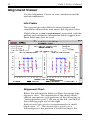
Alignment Viewer
92
Info Fields
Alignment Chart
Window Settings & Help
Deviation Chart & Notes Box
92
92
93
94
Live Eyes
95
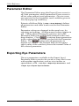
Parameter Editor
97
Exporting Eye Parameters
97
Parameter Fitter
98
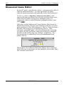
Measured Gaze Editor
102
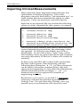
Importing Clinical Measurements
103
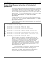
Exporting Measurements & Simulated positions
105
1999.09.04
Contents
vii
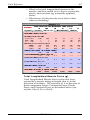
Mechanical State Viewer
106
Muscle Forces
106
T o t a l L o n g it u d in a l M u s c le F o rc e (g )
R o t a t io n a l M u s c le F o rc e (g )
U n it M o m e n t V e c t o r (% )
R o t a t io n a l F o rc e c o m p o n e n t (g )
107
108
109
109
Exporting Mechanical States
111
Point of View
112
Graphic Eyes
113
Other Issues
115
Names
Speed
Printing
Shortcuts
115
115
116
117
Trouble
118
Solutions Could Not Be Found...
Not Enough Memory
118
120
Frequently Asked Questions
122
How do the various Preferences and Window Settings differ?
Where are normal muscle insertion coordinates?
How do I make an Orbit Movie?
How do I Print Orbit Windows?
When Credit is Due
122
123
123
124
125
Ma t h e ma t i c a l An a l y s e s
127
Rotational Force due to Muscle Width
127
An n o t a t e d Or b i t Bi b l i o g r a p h y
133
Current Work
133
Overview of Our Research Program
134
Biomechanical Models of Eye Alignment
136
Studies of Eye Muscle Forces, Paths & Pulleys
138
Clinical Application of Biomechanical Modeling
146
Spin-Offs
149
L i t e r a t u r e Ci t e d
151
Or d e r F o r m & L i c e n s e Ag r e e me n t
155
1999.09.04
viii
Orbit 1.8 User’s Manual
1999.09.04
Preliminaries
1
Preliminaries
What is Orbit™?
The complexity of extraocular muscle coordination has
long confused and frustrated students, researchers, and
clinicians.
Orbit is a unique educational and research tool that
provides easy access to a sophisticated biomechanical
model able to simulate classical strabismus syndromes
and data from individual cases, thereby clarifying
diagnostic and treatment possibilities in well-defined
physiologic terms.
Orbit is used all over the world:
• Ophthalmologists, Optometrists, and Orthoptists use
Orbit to model complex cyclo-vertical and
innervational disorders, refining diagnostic and
treatment-planning skills.
• Researchers in vision and oculomotility use it to
study orbital mechanics in humans and non-human
primates, for instance, to distinguish orbital from
central determinants of oculomotor phenomena.
• Teachers supplement the ophthalmology curriculum
with self-paced strabismus simulation laboratories.
• Students working with Orbit are better able to
consolidate loosely connected facts and observations
into a solid sense of how the extraocular muscles
work.
Orbit is a tool for analysis of extraocular mechanical
and innervational factors in eye alignment. It contains
a pair of model eyes you can modify to reflect supposed
causes of motility disorders and proposed treatments,
and a simulated eye alignment test, which shows how
the modified eyes behave. Orbit is used to create
models of extraocular disorders and treatments,
observe their effects on eye alignment, and understand
the reasons for those effects in well-defined
biomechanical terms.
1999.09.04
2
Orbit 1.8 User’s Manual
Orbit is used in a trial-and-error mode: Beginning with
a pair of simulated normal eyes, you (1) alter one or
both to reflect your ideas about diagnosis or treatment,
(2) compare Orbit’s simulated alignment with clinical
alignment measurements or desired treatment
outcome, (3) repeat until you’re satisfied with the
match. A Parameter Fitter helps refine the trial-and
error process. Essentially, Orbit clarifies your
hypotheses, shows you their implications, and provides
a biomechanical analysis of your ideas. It does not
replace your judgment and experience in proposing
diagnoses and treatments.
In experimenting with diagnoses you can incorporate
whatever you know or suspect: perhaps you know that
you are dealing with a traumatic superior oblique
muscle (SO) palsy, but are unsure of the degree of
recovery and of secondary changes in other muscles. In
experimenting with treatments you can allow for visual
status, general medical status, lifestyle, etc. You are
free to make the tradeoffs your experience suggests:
Perhaps primary position is most important in one case
and reading position in another.
Orbit’s model eyes are biomechanical: they are modified
by changing properties, such as innervations, globe
dimensions, and muscle insertions, lengths, stiffnesses,
and contractile forces. Thus, Orbit is related to the
ophthalmotropes of Ruete (1845), Wundt (1862), and
others, its main advantage being that its behavior is
constrained only by knowledge of orbital mechanics,
and not by the materials and mechanisms feasible in a
physical model.
For each gaze angle, Orbit pursues iterative solutions
involving extraocular connective tissues, and the
innervations, paths, and tensions of all muscles in both
eyes, according to equations given, in part, by
Robinson (1975) and Miller and Robinson (1984).
Orbit is a Macintosh™ computer program, and has
been designed to operate in the consistent, natural way
typical of Macintosh programs.
1999.09.04
Preliminaries
3
Concerning Medical Use
Though based on the best data and analyses available,
Orbit is not approved for and should not be relied on
for decisions about patient care. Orbit is not intended
to substitute for any established diagnostic or treatment
planning procedure.
First, we are only beginning to understand extraocular
muscle cooperation in terms compatible with the
physical sciences, that is, on a biomechanical level. The
field is just emerging from the “schools of thought”
stage, where knowledge and practice are organized
around prominent teachers, but little is understood in
terms of generally accepted first principles (Kuhn,
1970). Second, orbital and brain physiology of a
particular patient may differ from the normal
population values in the model. Finally, Orbit has not
been widely tested against actual patient data.
What is Orbit Not?
There are two other, fundamentally different types of
models that have been used in strabismus analysis:
empirical generalizations, and expert systems.
Orbit contains no pre-programmed demonstrations of
syndromes (eg: Bregman, Ly and Galetta, 1991) and no
tables of surgical dose-response relationships (eg:
Parks, 1975). Such empirical generalizations are only
useful in “typical situations”, and do not help
understand underlying mechanisms. Instead, Orbit can
produce strabismus demonstrations, and derive doseresponse relationships.
Orbit is not an expert system. An expert system is a
model, not of the topics of interest themselves
(innervations, muscles, etc), but of the inferences and
judgments of human experts. One could create as
many different strabismus expert systems as there are
strabismus experts!
Indeed, Orbit knows nothing about strabismus, except
insofar as strabismus can be modeled as failures of
normal binocular coordination.
1999.09.04
4
Orbit 1.8 User’s Manual
Is Orbit Difficult to Use?
Yes and no.
As a Macintosh program, Orbit is simple and easy to
use. If you know a few other Mac programs, learning
Orbit will be easy.
However, if you are new to biomechanical analysis,
you may find it quite unlike your current approach to
strabismus. Although you will not need to learn
mechanics, mathematics, or anything not in this
manual, you will need to sharpen your analytic
thinking in several areas, as you will see.
Why bother? If you believe biomechanical analysis to
be an academic exercise or passing fad, you will
probably not want to make the effort necessary to
understand this new approach. However, if you are
concerned that strabismology in its current form may
not be equal to coming technical, economic and
competitive demands, you should waste no time in
adding this new tool to your armamentarium. So far as
we know, biomechanical modeling offers the only
coherent, scientific approach to problems of eye
alignment.
1999.09.04
Preliminaries
5
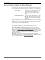
Conventions Used in this Manual
We will refer to items from the Menu Bar (at the top of
the Macintosh screen) with the » symbol. For example:
» File » New
means move the cursor to the
File item on the Menu Bar,
then click and drag to select
New.
»
» About Orbit™
means move the cursor to the
item on the Menu Bar, then
click and drag to select About
Orbit™.
In the Tutorial section of the manual, we use a pointing
finger ☞ to indicate actions you should take to follow
the example on your Macintosh.
The digital graphics in this Manual are in color,
although printed copies are grayscale, for reasons of
cost. Color PDF (Portable Document Format) files are
provided on the Orbit CD-ROM (see below) and on our
Website at www.eidactics.com/Software. Web editions
will be updated, as indicated by fractional edition
numbers (eg, 1.1).
PDF files can be viewed and printed with Adobe®
Acrobat® Reader, provided on the Orbit CD-ROM, and
also available online at www.adobe.com.
1999.09.04
6
Orbit 1.8 User’s Manual
We Did Not Do This Alone
Development of Orbit’s graphical interface has been
supported in part by The Smith-Kettlewell Eye
Research Institute, San Francisco, CA.
The underlying biomechanical model, and the
physiologic research on which it is based continues to
be supported by National Institutes of Health/
National Eye Institute grant EY06973 to JM Miller at
Smith-Kettlewell, and EY08313 to JL Demer at Jules
Stein Eye Institute, UCLA and JM Miller at SmithKettlewell.
For more about those involved in this project, launch
the Orbit application and select » » About Orbit™.
Eidactics, Orbit Gaze Mechanics Simulation and Orbit
are trademarks of Eidactics, San Francisco CA. For
timely information about Orbit, visit us on the Internet
at www.eidactics.com .
Macintosh, Power Macintosh, Mac, the MacOS logo,
System 8, Balloon Help, and MacApp are trademarks of
Apple Computer, Cupertino CA. Mac and the Mac OS
logo are used under license.
Unix is a trademark of AT&T.
1999.09.04
Preliminaries
7
Required & Recommended
To run Orbit, we recommend a Power Macintosh™
computer (which use 601, 603, 603e, 604, 604e, 750 or
G3, or G4 processors).
Orbit will run on a pre-PowerMac (sometimes called a
“68K” Mac, because it uses a Motorola 68000 series
processor) that has a math coprocessor and, at least,
MacOS 7.5.5, but it will run very slowly (see page 115).
We anticipate that the next version of Orbit will run
only on PowerMacs.
If you are using MacOS 8.0 you must also install some
system extensions that are included with the Orbit
distribution materials -- see the Orbit 1.8 Release Notes.
You may also install these extensions into MacOS 8.1,
but must not install them into any other MacOS
version.
Your computer must have at least 8MB of RAM
available to Orbit, and so at least 16 or 32 MB total, and
at least 256 color graphics.
No Windows™ version of Orbit is available or planned.
It is simply too difficult to support evolving software
on multiple platforms.
This manual assumes that you know how to use a
Macintosh. The Macintosh Tutorial, which came with
your system, teaches basic Mac skills. Your Macintosh
User’s Manual, and Macintosh online Help can also be
consulted about basic operations and terminology.
This Manual also assumes that you know the basics of
oculomotility and strabismus.
1999.09.04
8
Orbit 1.8 User’s Manual
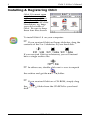
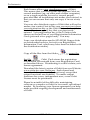
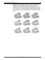
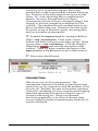
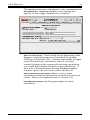
Installing & Registering Orbit
Orbit 1.8 cannot open
simulations created
with versions of Orbit
older than 1.5. If you
plan to work with older
simulations, eg, keep
your old version of
Orbit. Be sure to keep
these four files shown:
To install Orbit 1.8 on your computer:
☞ If you received Orbit on floppy diskettes, drag the
contents of the 2 or 3 diskettes to your hard disk:
If you received Orbit over Internet, you will instead
have a single archive file:
☞ In either case, double-click Orbit™ 1.8.sea to unpack
the archive and get the
folder.
☞ If you received Orbit on a CD-ROM, simply drag
the
disk.
folder from the CD-ROM to your hard
1999.09.04
Preliminaries
9
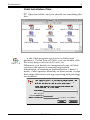
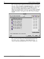
Orbit Installation Files
☞ Open the folder, and you should see something like
this:
... is the Orbit program (application in Macintosh
parlance). To run (launch) Orbit, you can double-click
this icon, drop a simulation file on it, etc.
Whenever you launch an unregistered copy of Orbit,
you have the option of entering registration
information, or running in demonstration (“demo”)
mode. Orbit operates normally in demo mode, except
that output functions (saving, exporting and printing)
are disabled.
1999.09.04
10
Orbit 1.8 User’s Manual
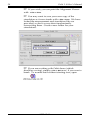
If you have purchased an Orbit license (see the Order
Form & License Agreement near the back of this
Manual), you will have received a card containing your
registration information:
Enter all four lines as shown on the card. The
registration key is always exactly 10 upper-case English
letters. If you misplace your registration information,
we can provide it from our files.
... is a description of improvements in, and
limitations of, the new version. Adobe Acrobat
Reader 3 or better (provided on CD-ROM, and
available free from Adobe at www.adobe.com) is
needed to read it.
The following 3 files are used by Orbit. Most users will
not deal with them directly. Be sure to keep them
together with Orbit in the same folder.
... is the standard set of normal eye parameters used by
Orbit. When Orbit is launched, Orbit_Norm is read in
as the description of normal eyes. When a new
simulation is created, parameters from Orbit_Norm are
1999.09.04
Preliminaries
11
stored as starting values in the new document. Factory
Settings for all Preferences are also stored in this file
(this allows you to return to these standard settings,
whenever you wish).
It is possible for knowledgeable users to modify
Orbit_Norm (it is a plain text file) to incorporate new
data about normal eye mechanics, or create versions for
different ages, races, sexes, and species. (If you do this,
be careful to only change values of existing parameters,
or add comment lines). If you alter Orbit_Norm, or
replace it with a new version, remember that only
newly created simulations will reflect the change.
Existing simulations that are opened or modified will
not. Orbit will complain when it is launched if it does
not find Orbit_Norm in its folder.
... stores your Preferences for New Simulations, that is,
the settings you make (as explained below) to
customize the way Orbit creates new simulations (it
initially stores standard Factory Settings). You can
create different sets of preferences for different users:
simply swap the desired Orbit_Prefs into Orbit’s folder.
If there is no Orbit_Prefs file in its folder, Orbit will
create one with Factory Settings.
Orbit_Prefs also stores your registration information. If
you wish to give a copy of Orbit to a colleague, give
him or her everything in this folder except for
Orbit_Prefs.
... holds Point of View settings (discussed below). If
there is no Orbit_POV file, Orbit’s Point of View
window will not show named points of view.
... contains items you may need to put into your
System Folder. If you are using MacOS 8.0 or 8.1,
open this folder and drop the contents onto your
closed System Folder. Let the Finder put the three
items contained in their proper places. Then
restart your computer and launch Orbit again. Do
not install these items into any system version
other than 8.0 or 8.1.
1999.09.04
12
Orbit 1.8 User’s Manual
Other files and folders in
contain simulations
of strabismic disorders, and related files, some of which
are referred to later in this manual.
Adobe Reader is needed to read the digital version of
this Manual, and the Orbit Release Notes. We include
the 4.0 installation kit on the CD_ROM, because earlier
versions seem to crash MacOS 8. For the current
version of Adobe Reader, see www.adobe.com.
If Orbit complains that your computer does not have
necessary hardware or software, then either your
MacOS System version is too old (remember: Orbit has
been tested only with MacOS 7.5.5 and later; you may
be able to upgrade your OS), or your computer is
inadequate. Some old Macs (eg, MacIIsi) may not have
math coprocessors, and cannot run Orbit.
As you work with Orbit, you will create new simulation
files (the generic Macintosh term for which is
documents); you may put these anywhere (Orbit Demo
does not allow simulations to be saved).
Cleaning Up
☞ The archive file or files (Orbit™ 1.8.sea...) you may
have are no longer needed. Drag them to the Trash to
complete the installation.
☞ If the various Orbit files do not have their icons,
shown below, or if double-clicking an Orbit simulation
fails to open it with Orbit, you must rebuild your
Macintosh desktop. To do this, restart your Mac, while
holding down the Command and Option keys.
Sharing Orbit with your Colleagues
As an Orbit licensee, you are free to share Orbit with
your colleagues, within the terms of your License
Agreement.
1999.09.04
Preliminaries
13
Each license allows one simultaneous use of Orbit.
This means that you may install and register Orbit on
several machines (eg, an office and a home computer)
or on a single machine for use by several people,
provided that all installations are under your control, in
that you can ensure that only one copy is in use at any
time.
You may also distribute copies of Orbit that will not be
under your control, but in this case you must not share
your registration key or the Orbit file (see below) that
contains an (encrypted) key that you previously
entered. Your registration key is the 10 letter code
shown on the last line of your Registration Information
Card (pictured a few pages back). You may:
Loan your distribution media (CD-ROM, floppy disks
or downloaded archive, but not your Registration
Information Card, which may have been included with
the distribution media).
Copy all the files from the folder
, except for
the file
. Orbit_Prefs stores the registration
information you entered from your Registration Card,
as described above. Distributing it would violate your
license agreement.
Download the latest version of Orbit from our Website:
www.eidactics.com/Software. Such shared and
downloaded copies are fully functional, except that
output functions are disabled. To enable output
functions for a new, independent user, a new Orbit
License must be purchased.
Please be mindful of the difficulty maintaining
software as complex as Orbit for our small, specialized
market. By honoring your license agreement you help
make possible ongoing development and maintenance
of Orbit.
1999.09.04
14
Orbit 1.8 User’s Manual
Click for Help
Helpful information embedded in a program is
particularly useful: it is there when you need it, and can
be context sensitive: you don’t have to search for the
topic you’re having a problem with, because the
program knows where you are.
Orbit provides three kinds of help.
Window Help Buttons
Many Orbit windows contain a help button. Click it for
a description of the window.
1999.09.04
Preliminaries
15
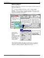
Balloon Help™
Balloon Help lets you point to an object on the screen to
find out what it is.
☞ To turn on Balloon Help, select
» Help » Show
Balloons. Then, point to an object in the menu bar or in
an Orbit window (titles, labels, buttons, ...) to find out
what it is and how to use it.
Orbit help
balloons tell
about
strabismus and
bio-mechanical
modeling, as
well as about
using Orbit.
Turn Balloon Help on when you first use a window,
and when you do not understand a menu selection,
window, field or button. Then turn it off.
1999.09.04
16
Orbit 1.8 User’s Manual
Help on the Menu Bar
When Orbit is active, several
short discussions are available
online by clicking Help in the
Menu Bar at the top of your
Macintosh screen:
» Help » What is Orbit™? contains
an overview.
» Help » Not Enough Memory suggests things to try when
Orbit (or any other Macintosh application) makes this
complaint.
» Help » Bibliography. An annotated bibliography of
scientific papers in which the biomechanical model
underlying Orbit, the basic research supporting the
model, and some clinical applications are discussed.
» Help » Ordering Orbit™ tells how to purchase Eidactics
products.
1999.09.04
A Biomechanical Approach
17
A Biomechanical Approach
to Strabismus
Clarification is one of the aims of our biomechanical
approach, so it would be ironic if a mysterious
physiologic system were simply replaced by a
mysterious computer program. It is important to
understand something about the foundation and inner
workings of Orbit.
The most important thing for you as a user to know is
what is included in Orbit’s calculations and what is not.
A biomechanical model such as Orbit is “minimalist” in
the sense that it does automatically only those
calculations that necessarily follow from specified
variables and parameters. Effects that may occur in
only some cases, or for which there is no clear
mechanism, cannot and should not be automatically
computed. Instead, Orbit allows you to explicitly test
hypotheses about such effects.
Orbit includes models of:
• muscle force (including elastic and contractile force
components),
• muscle path (including muscle length),
• Hering’s Law, which determines innervations to an
eye moving “passively” or “under cover”, given the
position of the fixing eye and the parameters of both.
• Sherrington’s Law of reciprocal innervation, which
relates innervations to paired antagonistic muscles.
Orbit does not include any models of central or
peripheral adaptive processes, or of post-surgical
healing. However, you can make hypotheses about
these processes, express them in Orbit’s biomechanical
parameters, and derive their implications. Similarly, it
cannot know the details of surgical technique (eg, how
much tendon is lost in muscle recession), but you can
express your estimates in terms of Orbit parameters.
Robinson (1975) and Miller and Robinson (1984)
describe the mathematical analysis on which Orbit is
based. This framework is fleshed-out with data on
1999.09.04
18
Orbit 1.8 User’s Manual
extraocular geometry, muscle paths, muscle crosssections, muscle forces, and elasticities.
We use a description of normal orbital geometry
derived from dissections of Volkmann (1869), serial
sections by Nakagawa (1965), and MRI studies by Clark
(Clark, et al, 1997). Muscle paths and cross-sections are
derived from MRI studies of Miller, Demer, and
colleagues (Miller, 1989; Miller, et al, 1993; Demer, et al,
1994; Demer and Miller, 1995).
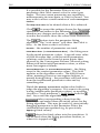
Parameters and Variables
We will use the term parameters or eye parameters to
refer to values that characterize an eye and do not
change as a function of eye position. A muscle’s origin,
stiffness and resting length are all eye parameters.
All other Orbit values, which can vary as a function of
eye position, are variables. Elastic muscle force and
muscle path length are examples of variables. Note, eg,
that stiffness (change in force / fractional change in
length), is an independent, intrinsic muscle property,
that is, a parameter, whereas elastic force, a variable,
depends on stiffness, muscle resting length and muscle
path length. The length of the path over which a
muscle travels depends on the shape of the path, which
depends on eye position, total muscle force and pulley
stiffness, among other things.
Fixing and Following Eyes
We use eye alignment and binocular alignment to refer to
phoria, not tropia. This follows from the fact that Orbit
treats biomechanical factors only, and knows nothing
about such sensory factors as fusional range. Thus,
when we talk about alignment, you should imagine
some test of eye alignment that completely dissociates
the two eyes in the sense of providing no binocular
visual alignment cues.
It is essential to know which eye is the fixing eye, the
eye voluntarily turned by the subject to point in a
known direction, and which eye is the following eye, the
eye which is moving under the influence of
innervations determined by the fixing eye, “passively”
or “under cover”. The Hess and Lancaster tests
approximate this ideal situation.
1999.09.04
A Biomechanical Approach
19
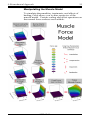
Muscle Force Model
Muscle force is calculated as the sum of a contractile
force, an elastic force, and a fixed force (useful in
simulating traction tests, in which an eye is rotated with
forceps). Contractile force is mainly a function of
innervation, but is also a function of fractional length
change or stretch, consistent with the sliding filament
model. Elastic force is a function only of stretch.
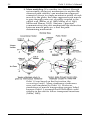
Consider a “simple” muscle resection. The mechanics
of this common procedure are more complex than you
may think, but since Orbit understands how eye
muscles work, much of the complexity is taken care of
automatically. To simulate resection correctly, you
need to know what happens automatically and what is
left to your judgment.
A modest resection may only remove tendon.
To perform a 5mm RLR resection, you would change
the Tendon Length from 8.4, shown above, to 3.4.
What are the mechanical implications?
First consider the operated eye fixing. When the
operated eye is fixing a given position, say, primary
position, the RLR will be more stretched than it was
before surgery. Orbit computes the increased stretch,
1999.09.04
20
Orbit 1.8 User’s Manual
increased elastic, and altered contractile force
components of the RLR. It then computes the forces in
the antagonist RMR and other muscles of the right eye
needed to hold the eye in primary position, and the
innervations needed to produce the contractile
components of these forces. Having computed right
eye innervations, Orbit uses its notion of Hering’s Law
to compute innervations to the following left eye, left
eye muscle forces, and, finally, left eye position.
With the operated right eye following, innervations,
determined by the unoperated fixing eye, are assumed
unchanged from before surgery. Resection alters RLR
forces, and so the right eye’s position. Orbit calculates
the new forces and eye position, as well as more subtle
things, such as changes in muscle path shape and
translational globe position.
Note that if you disinsert a muscle, cut off 5mm, and
sew it back to the original scleral insertion, Orbit cannot
know that you lost 1mm during disinsertion and took a
1mm “bite” of the remaining tendon during reinsertion.
In this case, you actually did a 7mm resection, and
must reduce Tendon Length from 8.4 to 1.4 mm.
Now, suppose we resect more than the tendon length,
shorten the muscle proper.
Elastic Force ("stiff" vs "soft")
Resection shortens a muscle, and a short muscle is said
to be “stiff”. What does this mean?
Imagine taking a 10 mm rubber band (resting length =
10 mm), and extending it by 10 mm (path length = 20
mm; fractional stretch = (20 - 10) / 10 = 100%). Then
cut off half of the band (resting length = 5 mm) and
again extend it by 10 mm (stretch = (15 - 5) / 5 = 200%).
It's harder to hold extended now because fractional
stretch is higher. Each unit length of the band is now
stretched to 3 times its resting length, compared to 2
times before it was cut.
Cutting a piece off the band did not change its intrinsic
properties – the band is still made of the same rubber
material and has the same cross-section. Similarly, the
intrinsic stiffness of a muscle is determined by the
nature of the elastic properties of the tissue (eg, its
fibrous content) and its cross-section, and is measured
in grams/fractional stretch. Cutting off a piece of
1999.09.04
A Biomechanical Approach
21
muscle, changing its resting length, only changes the
fractional stretch of the muscle (eg, from 100% to 200%)
for a given absolute movement of its end (eg, 10 mm),
thereby changing its elastic force.
We describe elastic muscle stiffness in terms of
fractional or percent change in length because then
stiffness is an independent parameter, not dependent
on resting muscle length. If we instead defined muscle
stiffness in terms of absolute stretch (mm), it would
change with resection. So, when one says, “a short
muscle is stiff” one is using a different meaning of
stiffness than we do here. We would say instead that a
short muscle must be stretched more than a long
muscle to cover the same path, and so, exerts more
elastic force.
Orbit can also be used to simulate and test your
hypotheses about changes in muscle cross-section (eg,
hypertrophy or atrophy) or tissue properties (eg,
fibrosis), which may occur over time in a resected
muscle or its antagonist. Such “secondary” changes
cannot be calculated automatically, however, because
they are not, so far as we know, necessary
consequences of resection and, in any case, little is
known about their determinants. Orbit simulation is
currently the only practical way to test such clinical and
scientific hypotheses.
Contractile Force ("strong" vs "weak")
Contractile force depends mostly on innervation, which
causes each sarcomere (one of the serial contractile
elements of a muscle fiber) to shorten. There is also a
length dependency intrinsic to the sarcomeres: they
have an optimal length for force generation. Stretched
or crushed sarcomeres develop less force at given
innervations. The contractile force model built into
Orbit automatically reflects these effects.
Orbit also provides parameters with which you can
alter each muscle’s response to a given level of
innervation.
Orbit does not, for reasons that should now be clear,
automatically calculate central innervational
adaptations that might follow from strabismic lesions
or muscle manipulations. This makes it a useful tool
for testing hypotheses about such adaptational
mechanisms.
1999.09.04
22
Orbit 1.8 User’s Manual
In summary, removing a length of muscle affects both
elastic and contractile components of muscle force:
• A resected muscle exerts more elastic force at a given
length, and so, roughly speaking, at a given eye
position. This effect is most significant when the
muscle is elongated, that is, out of the muscle’s “field
of action”. It is in this sense only that a resected
muscle is “stronger”.
• Resection of a muscle that removes contractile tissue
leaves the muscle less effective in contracting. A
given change in innervation results in less change in
path length, and the range of lengths over which the
muscle can effectively operate (recall the sliding
filament model) is reduced. These contractile effects
are most important in a muscle’s field of action.
So, with respect to the above discussed effects of
muscle manipulation, you specify the surgery (and any
muscle abnormalities), and Orbit does the rest.
Secondary Effects of Surgery
As we have seen, resection stretches a muscle, forcing
its sarcomeres to operate at longer than optimal
lengths. Conversely, recession slackens a muscle,
forcing its sarcomeres to operate at shorter than
optimal lengths. It has been found that, within a few
weeks or months, resected muscles actually add
sarcomeres, and recessed muscles delete sarcomeres,
thereby allowing the remaining serial sarcomeres to
operate at their optimal lengths (Tabary, et al, 1972;
Williams and Goldspink, 1973; Williams and
Goldspink, 1978; Scott, 1994).
However, muscle length adaptation is not well enough
understood to be incorporated as automatic Orbit
calculations. To predict long-term eye alignment, you
must make your own hypotheses about such secondary
muscle length changes, and enter your estimates into
Orbit. In the Tutorial section, below, we will show how
this might be done.
Even less is known about post-surgical modifications of
innervation and about fibrotic and atrophic changes
that may occur in some situations. As with secondary
muscle length changes, you can enter any such changes
you suspect, and Orbit will deduce their consequences.
1999.09.04
A Biomechanical Approach
23
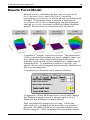
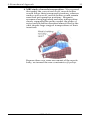
Manipulating the Muscle Model
To simulate abnormalities, treatments, and effects of
healing, Orbit allows you to alter parameters of the
muscle model. Various scaling and offset operations on
the normal force surfaces are available:
1999.09.04
24
Orbit 1.8 User’s Manual
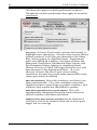
Innervation threshold (called offset in the figure),
innervation sensitivity and contractile (muscle) strength
allow the normal contractile muscle force surface to be
customized.
• Innervation threshold slides the contractile force
surface along the innervation axis, so that, eg,
contractile force first appears at lower innervations
for decreased thresholds, and saturates at
innervations the same amount lower. Eg, if you
have reason to think that neuromuscular junctions
are weakened, increase innervation threshold.
For a simple example, change the innervation
threshold of a muscle in the following eye (Expert
Parameter Editor) and note (in the Mechanical State
Viewer) that innervation does not change (ie, the
sensitivity of the muscle is affected, not the
brainstem’s output), but the contractile muscle force
does change.
• Innervation sensitivity squashes (or stretches) the
muscle force surface along the innervation axis, so
every change in innervation behaves like a larger (or
smaller) change on the normal surface. Myasthenia,
eg, might be modeled by decreasing innervation
sensitivity.
• Contractile muscle strength scales the vertical (force)
axis. A large muscle with more contractile fibers in
parallel than normal would be modeled by
increasing contractile muscle strength.
Expert note: Your Parameter Editor shows
Contractile Muscle Strength and Contractile Muscle
Relative Strength. Normally, the former values are
all 100%, and the later give contractile forces relative
to the lateral rectus muscle (LR). The two
“strengths” are separated so you can think about
changes with respect to either a muscle’s normal
strength alone, or relative to other muscles.
Internally, the two values are simply multiplied, so,
eg, doubling either has the same effect.
Stretch sensitivity and elastic strength allow the normal
elastic muscle force surface to be customized.
• Stretch Sensitivity squashes the Elastic Force Surface
along the stretch axis. A fibrotic muscle, which hits
asymptotic stiffness (the leash region) at low values of
stretch, would be modeled by increasing Stretch
Sensitivity.
1999.09.04
A Biomechanical Approach
25
• Elastic Strength scales the vertical (force) axis. A
large muscle with more elastic fibers in parallel than
normal would be modeled by increasing elastic
muscle strength.
Expert note: Your Parameter Editor shows Elastic
Muscle Strength and Elastic Muscle Relative
Strength. Normally, the former values are all 100%,
and the latter give elastic forces relative to the LR.
The two “strengths” are separated so you can think
about changes with respect to either a muscle’s
normal strength alone, or relative to other muscles.
Internally, the two values are simply multiplied, so,
eg, doubling either has the same effect.
The values of muscle forces and the rotational stiffness
of non-muscular orbital tissues are derived from
intraoperative and other measurements of Collins, et al
(1975; 1981).
Translational stiffness of the globe, important in
simulating restrictive and co-contractive syndromes, is
estimated from the data of Dyer and Henderson (1958).
Hering's Law of Equal Innervation is simulated by
converting innervation sets of the fixing eye into
equivalent (with respect to a normal eye) gaze angles,
reflecting the gaze angles across the midline, and
converting back into innervation sets. This procedure
is schematized in the Test of Binocular Alignment section
below.
Sherrington's Law of Reciprocal Innervation is hardcoded, as described by Robinson (1975). It may be
possible, in a future version of Orbit, to solve for each
of the 6 innervations in a set independently, thereby
simulating, rather than assuming, the exact form of
reciprocal innervation.
1999.09.04
26
Orbit 1.8 User’s Manual
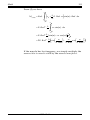
Basic Data and Operations
Orbit operates on three types of data: innervations, gaze
positions, and eye parameters, solving a force-balance
equation to determine innervations from positions and
parameters, or positions from innervations and
parameters. These two types of solutions answer two
types of questions:
(1) What innervation set is required to drive a given eye
to a given position?
(2) To where will a given eye move if supplied with a
given innervation set?
Eye parameters include locations of muscle origins and
insertions, muscle and tendon dimensions, innervationlength-tension relationships, and elastic properties of
ocular fat and fascia. Innervations to the six muscles of
each eye are given in arbitrary units. All three
components of eye rotation are specified: abduction,
supraduction, and excyclotorsion. Eye translation,
significant in some disorders, is calculated as well.
Find
Ï
Position
Find
Innervation
Set
Parameters
Innervation
Set
Position
Fit
Parameters
Finding innervations and positions is relatively
straightforward. However, clinical application needs
the ability to find eye parameters. Finding eye
parameters corresponds to making a diagnosis or
choosing a treatment. Finding the parameters of eyes
that show a given pattern of misalignment, or how eye
parameters must be altered to restore good alignment
is a trial-and-error process.
1999.09.04
A Biomechanical Approach
27
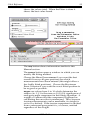
New in Orbit 1.8 is the Parameter Fitter, which
automates the trial-and-error process. In some cases,
then, Orbit 1.8 can also answer the third question:
(3) What parameters describe eyes that will move to
desired positions under given innervations?
1999.09.04
28
Orbit 1.8 User’s Manual
Rectus Muscle Pulleys?
In the Orbit 1.8 model rectus muscles pass through
pulleys, located posterior to the equator, and elastically
coupled to the orbital wall. Soft rectus muscle pulleys are
a recent discovery, and since one might reasonably be
skeptical about claims of new, functionally significant,
gross anatomic structures in such a familiar part of the
body, we will review the findings.
Prior to the development of computational models of
extraocular biomechanics it seemed sufficient to
describe extraocular anatomy in terms of origins,
insertions, and cross-sections of extraocular muscles
measured in cadavers. But then several new results
appeared:
1. Modeling: The attempt to calculate binocular
alignment from first principles (Robinson, 1975;
Miller and Robinson, 1984; Miller, et al, 1984) made it
obvious that paths of EOMs and gaze dependence of
their paths could not be inferred from cadaveric
data, but had to be measured in alert subjects.
1999.09.04
A Biomechanical Approach
29
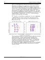
2. Imaging: These measurements were performed in
monkeys and humans by Miller, et al (1984),
Simonsz, et al (1985), Miller and Robins (1987), and
Miller (1989). The main finding of all these studies
was that rectus muscle bellies are remarkably stable
with respect to the orbital wall over the full range of
gaze.
1999.09.04
30
Orbit 1.8 User’s Manual
3. More modeling: We consider two distinct (though
not mutually-exclusive) mechanisms to explain the
observed path stability: one mechanism supposed
connective tissue to couple an anterior extent of each
muscle to the globe; the other supposed each muscle
to pass through some sort of pulley coupled to the
orbital wall (Miller, et al, 1984; Miller, et al, 1990;
Miller and Demer, 1992). Simonsz (“personal”
communication) has also emphasized the distinction
between muscle paths per se and the pathdetermining mechanism.
Orbit 1.0 was based on the first notion, the
conventional model. Many strabismus syndromes
were well simulated by Orbit 1.0. However,
simulations of muscle transposition surgery failed
because Orbit 1.0 assumed that EOM bellies could
sideslip in the orbit to follow transposed insertions
(Miller, 1985).
1999.09.04
A Biomechanical Approach
31
4. MRI study of muscle transposition: We reasoned
that under the conventional model, muscle bellies
would follow their transposed insertions, whereas
under a pulley model, muscle bellies would remain
near their pre-operative positions. Magnetic
resonance imaging before and after transposition
clearly supported the pulley model: the paths of
rectus muscle bellies remained almost fixed in the
orbit despite large surgical transpositions of their
insertions.
Because there was some movement of the muscle
belly, we termed the new constraints soft pulleys.
1999.09.04
32
Orbit 1.8 User’s Manual
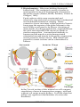
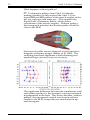
5. Histochemistry: What was holding the muscle
bellies back? We conducted a series of studies to
anatomically locate and histologically characterize
the pulley tissues (Demer, Miller, Poukens, Vinters &
Glasgow, 1995).
Fresh cadaver orbits were exenterated and
selectively step and serial sectioned for histochemical
and immunohistochemical staining. Dense
connective tissue structures within posterior Tenon's
fascia near the equator of the globe adjacent to the
recti EOMs were found to be sleeves consisting of
dense bands of collagen and elastin, suspended from
the orbit and adjacent EOM sleeves by bands of
similar composition. A monoclonal antibody to
human smooth muscle α-actin demonstrated
substantial smooth muscle in the pulley suspensions
and in posterior Tenon's fascia. Mid-orbital and
posterior coronal sections can be schematized as
follows:
In the Tutorial section of this manual we will compare
simulations of muscle transposition surgery, with and
without soft rectus muscle pulleys. It will be clear that
pulleys are significant determinants of extraocular
mechanics.
1999.09.04
A Biomechanical Approach
33
Again?
The notion of rectus muscle pulleys has arisen before,
apparently without the evidence needed to get a fair
hearing. As recounted by Scobee (1952), Lockwood
(1886) described a band of fibers imbedded in Tenon’s
capsule crossing the posterior edge of each opening
and called these bands the intracapsular ligaments. He
went on to describe several intracapsular and
suspensory ligaments later visualized by Koornneef
(1983). Ferrall proposed these structures acted as
pulleys, but Whitnall (1932) flatly stated that “there are
no pulley bars or intracapsular ligaments, and no need
for them” (so there!).
1999.09.04
34
Orbit 1.8 User’s Manual
What is a Simulation?
An Orbit document -- a set of fixations, eye parameters,
clinical measurements, etc -- is also referred to as a
simulation.
We provide several simulation examples in the folders
and
,
. We
will refer to them in the Tutorial section (page 47).
Existing simulations can be opened in all the usual
ways: From within Orbit, use » File » Open ; from the
Finder desktop, double-click on a simulation icon, or
drag-and-drop a simulation icon on the Orbit
application icon.
To begin a new simulation from within Orbit,
select » File » New.
When a simulation is open, it is listed in the » Simulations
menu.
A simulation is open if and only if one or more
simulation windows -- windows referring to a particular
simulation -- are open. Thus, some simulation window
always opens with a simulation (see
» Both Eyes » Preferences), and the simulation is closed
when its last window is closed.
Certain windows do not refer to any particular
simulation, and so are not simulation windows: These
are Preferences, Point of View, Converter, and all of the
windows.
You can have as many simulations open as memory
(the machine’s and yours!) permits.
1999.09.04
A Biomechanical Approach
35
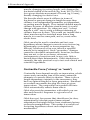
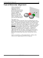
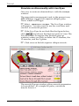
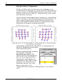
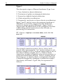
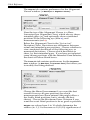
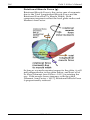
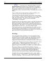
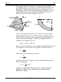
Test of Binocular Alignment
Orbit simulates the
common clinical
alignment tests in
which the two eyes are
dissociated (prevented
from seeing the same
targets), and the
patient fixates with
one eye as the other
follows passively. In
Orbit 1.8 either or both
eyes may be abnormal.
The figure is a
schematic of the Lancaster Test in which the eyes are
dissociated by viewing colored targets through colored
filters. The patient has been asked to fix the red bar at
(0,0), seen only by her left fixing eye, and to move the
green bar, seen only by her right following eye, so that it
appears to lie on top of the red bar. Assuming normal
retinal correspondence, the positions of the two bars
give the gaze angles of the two eyes. If binocular
alignment were normal, our patient would have
superimposed the two bars. In the case shown, her
right eye is 20° exo-deviated (misaligned outward), 5°
hyper-deviated (upward), and somewhat excyclodeviated (twisted top-outwards, around the visual
axis).
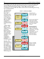
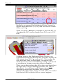
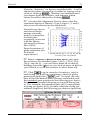
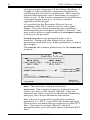
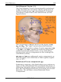
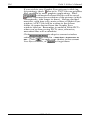
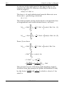
Orbit’s simulation, schematized below, follows the
clinical test, beginning with the fixing eye.
1999.09.04
36
Orbit 1.8 User’s Manual
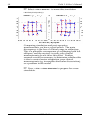
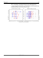
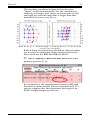
First (Figure part A), the operator Find Fixable Position calculates the
torsion that the (possibly abnormal) fixing eye would assume at a
chosen 2-dimensional gaze angle. Then, (B) with all 3 gaze
coordinates, we can find the innervations that would bring the fixing
eye to that position.
To implement
Hering's Law
(C), we use
Inner Eye
Parameters to
transform the
Innervation Set
to Fixing Eye
into “position
space”, reflect
the position
across the
midline, and
transform back
into
“innervation
space”. The
Inner Eye is
simply a third
set of eye
parameters
that is usually
left with the
normal values
supplied, but
may be
modified
(» Both Eyes »
Orbit™ 1.8 Binocular Model
A
Fixing Eye
Parameters
Find torsion for
arbitrary fixing eye
(new in Orbit 1.8).
Find Fixable
(3D) Position
Inner Eye
Parameters
Fixable
Position
B
Find
Innervation
Set
Fixing Eye
Parameters
Innervation set
to Fixing Eye
C
Inner Eye
Parameters
Find
Position
Intended Position
of fixing Eye
Reflect Eye
Position Across
Midline
Now we can find the 3
reciprocally-related
innervation pairs that
would drive the Fixing
Eye to the Fixable
Position.
But the 2 eyes are
mirror images (eg,
when the fixing eye
abducts, the following
eye adducts), so to get
Following Eye
Innervations, we must
“reflect” the Fixing
Eye Innervations
across the midline.
Intended Position
of Following Eye
E
Inner Eye
Parameter Editor).
Finally, (D)
this Innervation
Set to Following
Eye, and a
description of
the following
eye go to Find
Position, which
calculates the
position of the
following eye.
2D Gaze
Position
Find
Innervation
Set
Inner Eye
Parameters
Innervation set
to Following Eye
D
Following Eye
Parameters
Find
Position
Position of
Following eye
1999.09.04
Now it’s a simple
matter to find the
position of the
Following Eye.
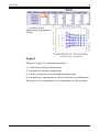
A Biomechanical Approach
37
If the fixing eye is normal, only the calculations in box
E are necessary (this was the total calculation in Orbit
1.0).
We can compare such a set of simulated gaze positions
with a set of clinical measurements, altering eye
parameters to optimize the fit.
The outcome of such a simulation is a diagnosis of the
patient's disorder in biomechanical terms. Similarly,
we can find the orbital manipulations that would cause
our model sick eye to assume normal, conjugate gaze
positions. The outcome of this simulation would be a
treatment plan. Many aspects of the model eye can be
manipulated in pursuit of a diagnosis or treatment.
The Parameter Fitter, described below, partially
automates the trial-and-error process.
Eye Position
Coordinates for Translation
The eye is cushioned in the orbit by elastic fat pads, so
it cannot only rotate, it can also translate slightly. For
most purposes we can ignore globe translation, but in
some restrictive and co-contractive syndromes, globe
translation is a significant factor, as we will see when
we analyze Duane’s syndrome. For now, we just note
that specifying translation is straightforward, since we
are all familiar with the conventional Cartesian
coordinate system for describing translational motion.
Orbit uses Cartesian coordinates fixed to the skull, with
origin at the point where the center of the globe falls
when the eye muscles exert no forces. The three axes
are oriented with a protrude-retract axis aligned with
the orbital axis, an upward-downward axis
perpendicular to the first and as close to vertical as
possible, and a sideward-middleward axis
perpendicular to the other two. The names used in
Orbit to refer to these axes are the names of the positive
directions:
sideward
Positive sideward movement is
translation toward the side of the head.
Sideward movement is not the same as
conventionally defined “lateral” or
“temporal” movement, because our
1999.09.04
38
Orbit 1.8 User’s Manual
coordinate system is turned outward to
align with the orbital axis.
protrude
Positive protrusion means the eye
bulges out of the orbit. Negative
protrusion, or retraction, is more
frequently spoken of in strabismus.
upward
The upward-downward axis is tilted
slightly from the common anatomic
superior-inferior axis, because our
coordinate system is pitched slightly
backwards to align with the orbital axis.
Only protrusion-retraction is of practical interest in
strabismus.
Rotation is more of a problem than translation, and it is
a deep problem: rotations are mathematically more
complex than translations, and further, these
complexities are of an unfamiliar kind. Below, we
discuss how eye rotation is described in Orbit.
Coordinates for Rotation
Any given 3-dimensional rotation can be described
with 3 numbers, or coordinates, by definition. There
are many correct rotational coordinate systems, and to
describe the rotation of an object like an eyeball, one
must first choose a system, on the basis of its
usefulness, familiarity, aesthetics, or something else. It
is important to understand that the same 3-D rotational
position may have different coordinate values when
described in different coordinate systems.
Two popular coordinate systems for eyes are Fick
coordinates and Helmholtz coordinates. The 3 Fick
coordinates are named longitude, latitude and torsion; the
3 Helmholtz coordinates are named elevation, azimuth
and torsion. Although the same term is used to describe
the third coordinate in both systems, Fick and
Helmholtz torsion are only qualitatively similar: they
both describe rotation about a visual axis, the direction
of which is determined by the first two coordinates.
But because the first two coordinates are different
(except in some special cases), torsion values describing
the same rotation are different, as well.
1999.09.04
A Biomechanical Approach
39
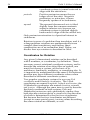
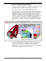
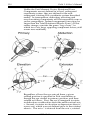
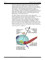
Orbit uses Fick rotational coordinates.
You may already be familiar with Fick coordinates as
the longitude and latitude lines conventionally drawn
on a globe of the earth. Imagine the eye at the center of
the globe, and its visual axis pointing at the intersection
of 0° longitude and 0° latitude (green arrow). First,
rotate the eye so that the visual axis moves along the
equator, until it points to, say, 40° longitude (yellow
arrow). Second, rotate the eye so that the visual axis
moves straight up the 40° longitude line, until it points
to the 20° latitude line (orange arrow). The longitudelatitude coordinates of the eye are, by definition, now
{40°, 20°}. Notice that the elongated dimension of the
arrow, which was parallel to the local longitude line at
{0°, 0°, 0°} and at {40°, 0°, 0°}, remains parallel at {40°,
20°, 0°}. This means that torsion in the Fick system is
zero. Of course, one more independent dimension of
rotation remains: without changing longitude or
latitude, you can rotate the eye about the visual axis. If
you rotated the eye, say, 10° about the visual axis (red
arrow, torsion exaggerated), its Fick coordinates would
be {40°, 20°, 10°}.
1999.09.04
40
Orbit 1.8 User’s Manual
We are also free to rotate the eye using a different
coordinate system. Imagine the way an astronomical
telescope is mounted: the telescope is attached to an
“azimuth” disk by a perpendicular axis that carries a
pointer. Rotating the telescope about the axis points to
angle markers drawn on the disk. The disk itself is
mounted so that it can be tilted up or down about some
axis. Such a mechanical arrangement follows the
Helmholtz system for describing rotation. First, from
some conventional starting position (the position that
we call straight-ahead gaze, {0°, 0°, 0°}), we elevate the
disk by, say, 40°. Second, we rotate the azimuth
pointer from 0° to 20°, and third, we twirl the telescope
-- or eye -- about its visual axis by, say, 10°. We are
now at Helmholtz coordinates {40°, 20°, 10°}. This is
not the same position as Fick {40°, 20°, 10°}! If you
doubt this, imagine the rotation {90°, 90°, 0°} in the two
systems.
Rotational Positions in Orbit
Before we can specify a rotational eye position we need
to choose a coordinate system and an origin, name each
coordinate, and decide which direction will be positive.
In Orbit, we use the Fick coordinate system, and take
primary position, straight ahead, as {0°, 0°, 0°}. The
reasons are partly historical, in that Robinson (1975)
used Fick coordinates, and partly practical, because
clinicians speaking about “horizontal” and “vertical”
eye movement, are usually, it seems, thinking of a
longitude-latitude system. Note that “horizontal” and
“vertical” are not well defined unless a coordinate
system is specified. In connection with Orbit
simulations, “horizontal” rotation will always mean a
change in longitude only, and “vertical” rotation will
always mean a change in latitude only, according to the
Fick coordinate system.
The term gaze is conventionally used to refer to the
direction of the visual axis only, that is, to horizontal
and vertical components, leaving torsion unspecified.
Thus, we specify intended gaze in Orbit simulations, and
fixing eye gaze in clinical eye alignment tests, because
patients are not asked to bring the fixing eye to a
specified torsional position, and indeed, without
special training (Nakayama and Balliet, 1977), they
cannot.
1999.09.04
A Biomechanical Approach
41
Finally, we have chosen coordinate directions that take
advantage of the mirror symmetry of the eyes: eg, we
use abduction-adduction instead of rightwardleftward. This allows us to describe gaze mechanics in
a way that is valid for either eye. We use coordinate
names that indicate which direction is positive:
abduction, elevation and extorsion:
abduct
or abduction, is the 1st Fick coordinate
rotation away from primary position.
Positive rotation about this vertical axis
moves the visual axis away from the
body’s midline, along the equator.
elevate
or elevation, is the 2nd Fick coordinate
rotation. It is rotation in the plane of the
local longitude (see “globe” figure
above). Positive rotation about this
horizontal axis moves the visual axis up
along a longitude line.
extort
or extorsion, is the 3rd Fick coordinate
rotation. It is rotation about the visual
axis, such that the top of the eye moves
laterally.
Deviations
It is useful to speak of a fixing eye and a following eye. In
some alignment tests, the following eye is actually
covered (and, so, is referred to as the covered eye), and
the patient voluntarily moves the fixing eye to various
standard gazes. In other tests, neither eye is covered,
but it is arranged that there is nothing visible to both
eyes, that is, that there is no fusional target. The
position of the following eye is ascertained as the
patient fixates standard gaze targets.
Deviations are differences between following eye and
fixing eye rotational positions. One might more
descriptively (and less humorously) call them
“misalignments”, but “deviations” is conventional.
exo-dev
or exodeviation = (following eye
abduction) + (fixing eye abduction).
The “+” appears because of the mirror
symmetry of the eyes. Exodeviation is
positive when the following eye is more
abducted than fixing eye is adducted
1999.09.04
42
Orbit 1.8 User’s Manual
hyper-dev
or hyperdeviation = (following eye
elevation) - (fixing eye elevation).
Hyperdeviation is positive when the
following eye is more elevated than
fixing eye.
excyclo-dev
or excyclodeviation = (following eye
extorsion) + (fixing eye extorsion).
The “+” appears because of the mirror
symmetry of the eyes. Excyclodeviation
is positive when the following eye is
more excyclorotated than the fixing eye
is incyclorotated.
Torsion, Of Course, Depends on the
Coordinate System
Torsion, as we have explained, is the third coordinate of
3-D rotation.
What is “normal” or “physiologic” torsion? We have
seen that 3 independent component rotations -- or 3
“degrees of freedom” -- are available for 3-D rotations.
Donder’s Law states that the eye position control system
uses only two degrees of freedom: torsion is not
independently controlled, and for each gaze, the
normal eye always assumes some particular torsion.
Listing’s Law tells what that unique torsion value is, that
is, Listing’s Law gives a torsion value for each pair of
numbers specifying gaze. We should not now be
surprised that the value of this normal or Listing torsion
depends on the coordinate system we use. Because of
the way a normal eye (or at least, one that obeys
Listing’s Law) rotates, it turns out that in both Fick and
Helmholtz coordinates, torsion is zero for pure
elevation-depression, and for pure abductionadduction (“secondary gaze”), but non-zero elsewhere
(“tertiary gaze). Further, when torsion is non-zero, it is
different in the two systems.
Interestingly, it turns out to be possible to define yet
another coordinate system, in which torsion for an eye
that follows Listing’s Law is zero everywhere. We find
these Listing coordinates useful when discussing how
extraocular connective tissue contributes to enforcing
Listing’s Law (see below), but not for much else.
Coordinated innervations, incidentally, provide the
other contribution, so if something is wrong with
1999.09.04
A Biomechanical Approach
43
extraocular tissues or with the brainstem, non-Listing
torsions can result.
Excyclo, short for excyclorotation, and the directionally
uncertain cyclorotation, are conventional terms for the
amount of torsion in excess of Listing torsion, that is,
for abnormal torsion. Cyclorotation describes single
eyes, and is zero at all gaze angles for normal eyes, by
definition.
Extorsion? Excyclo?? Excyclo-Dev?!?!
(If you’ve made it this far, you might as well push on to
the end of the section!)
There are three different notions in common use that
involve rotation of the eye about its visual axis. Often,
the concepts are not distinguished, or one term is used
indiscriminately. We distinguish the following terms:
Extorsion, as we have explained, is simply the third
coordinate of 3-D rotation, with a hint about the
positive direction.
Excyclo-Dev, or excyclodeviation, intrinsically involves
two eyes. Certain clinical tests of binocular eye
alignment, such as the Lancaster test, yield a value that
is the difference between torsions in the fixing and
following eyes. That is, with normal retinal
correspondence, the patient may place his red streak at
an angle to the examiner’s green streak, either because
his following eye has abnormal torsion (the usual,
possibly mistaken, presumption), his fixing eye has
abnormal torsion, or both. Such alignment tests
measure the difference between fixing and following
eye torsions. There is no conventional term to specify
this difference, so by analogy with “exodeviation” and
“hyperdeviation”, which refer to horizontal and
vertical misalignment of the following eye relative to
the fixing eye, we coin the terms cyclodeviation and
excyclodeviation, and the abbreviation excyclo-dev, to
refer to torsional misalignment of the following eye
relative to the fixing eye.
To summarize:
Torsion (extort) is rotation about the visual axis.
Listing Torsion (listing) is normal torsion according
to Listing’s law.
1999.09.04
44
Orbit 1.8 User’s Manual
Cyclorotation: excyclo = extort - listing.
Cyclodeviation: excyclo-dev = following eye extort +
fixing eye extort, where the “+” occurs because of
reflection across the midline).
The Mechanical State Viewer shows all of the values
mentioned for a given intended gaze. You may find it
helpful to review the above discussion while looking at
the Deviations and Eye Rotation values for a tertiary
gaze (eg, 30,20).
Limitations of Orbit
In Orbit 1.0 the fixing eye had to be normal. Orbit 1.5
and 1.7 did not require that the fixing eye be normal,
only that it obeys Listing’s Law, that is, has normal
torsion† . The following eye could be arbitrarily
abnormal.
With Orbit 1.8, this last restriction is lifted: the fixing
eye, too, may be arbitrarily abnormal.
The method used by Orbit 1.8, outlined in part “A” of
the Orbit 1.8 Binocular Model flowchart, above, is
similar to that described by Miller and Robinson (1984).
†
The reason for the Listing’s Law restriction in earlier versions can be
explained with reference to part “B” of the Lancaster Test simulation
flowchart. In part B we calculate innervations to the fixing eye. Find
Innervation Sets needs to be given all three coordinates (horizontal, vertical
and torsional) of each Fixing Eye Position and all Fixing Eye Parameters to
do its work. Generally, we specify only horizontal and vertical
components of the fixing eye position (as with the Intended Gaze Selector,
discussed below), and make some assumption about torsion: Our
assumption in Orbit 1.7 and earlier versions was that torsion of the fixing
eye was determined by Listing’s Law.
If the fixing eye had significant abnormal torsion, then Orbit’s assumption
of Listing torsion would produce errors in simulated following eye
positions. For instance, if the fixing eye were actually extorted (eg: SO
palsy), Orbit would still suppose, eg, that the medial rectus muscle (MR)
of the fixing eye had only horizontal action in primary position, and
innervate the following eye on that assumption. Actually, the MR of the
extorted fixing eye had developed some elevating action, requiring
general alteration of innervations to the fixing eye, and so by Hering’s
Law, to the following eye. Thus, the simulation of following eye positions
would have been in error.
1999.09.04
A Biomechanical Approach
45
PowerMac™ computers perform these computations
quickly. If you are using a Non-PowerMac, you will
need to be very patient, and pay close attention to the
issues discussed in the section of this Manual on Speed
115). We do not recommend you use Orbit on a NonPowerMac, except for evaluation.
1999.09.04
46
Orbit 1.8 User’s Manual
1999.09.04
Tutorial
47
Tutorial Examples
As with any tool, Orbit’s utility depends on your skill.
To show you how to work with Orbit, we will develop
several simulations. These simulations are saved in the
,
and
folders, for your examination.
We will point out the steps you should actually
perform on your Mac, if you wish to follow the
presentation.
1999.09.04
48
Orbit 1.8 User’s Manual
Superior Oblique Palsy
First, we will simulate a composite case of SO palsy, in
the course of which we will use many basic Orbit
functions. We will also see some of the strengths and
limitations of Orbit, and some of the limitations of
current methods of measuring binocular alignment.
We will also confront some gaps in our current
understanding of some muscle actions (topics for
future research). Recall that, where Orbit cannot
confidently perform a calculation, it does nothing. By
leaving such matters to the User, Orbit allows
hypotheses to be tested.
Launch Orbit
☞ Launch Orbit by double-clicking on the
icon. The Orbit splash screen appears:
Here you see:
• The Orbit version. Is this the version you intended
to run?
• Registration -- the person identified is responsible for
all use made of this licensed software.
1999.09.04
Tutorial
49
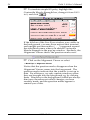
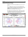
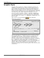
View the Alignment Pattern
If your copy of Orbit is factory-fresh, all of its
Preferences are set to standard, “factory” values. A
new simulation will open with the help window What Is
Orbit?, and the Alignment Viewer. Read this help window,
if you have not already done so.
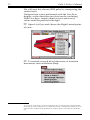
☞ Otherwise, to be sure you can follow the examples
below, close any open windows, select » Both Eyes »
Preferences for New Simulations..., click
, and then
:
☞ Then, create a new simulation with » File » New.
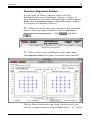
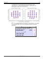
The Alignment Viewer will open. It should look like this:
On this Hess-Lancaster-type chart, each intended gaze
position is represented as a small black cross, “+”, in the
1999.09.04
50
Orbit 1.8 User’s Manual
intended position of the following eye, that is, the
position that would be assumed by a normal following
eye. Positions of the following eye are shown as blue
circles, “o”, with connecting lines to emphasize the
pattern. An arrow through each circle shows
cyclorotation (torsion in excess of normal Listing’s Law
torsion), as tilt from straight up, multiplied by 5 for
visibility. The simulated eyes are normal, because we
haven’t modified them yet. Therefore, the blue circles
lie exactly on top of the black crosses, obscuring them
until we introduce an abnormality.
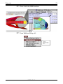
☞ Examine the Alignment Viewer by turning on Balloon
Help (» Help » Show Balloons). Point to the various
buttons and fields to discover what they are for. When
you are done, » Help » Hide Balloons. Click the Window
Help Button
, and read the description of the
window. There is a more complete discussion of the
Alignment Viewer in the Reference section of this manual.
☞ Enter some identification:
Intended Gaze
Why do we use intended gaze positions? The
conventional alternative would be to specify positions
of the fixing eye for comparison with the positions of the
following eye. But then, because of the mirror symmetry
of the eyes, calculating deviations requires interchanging
abduction and adduction and reversing the sign of
torsion for the fixing eye. When you represent
deviations graphically, as in a Hess-Lancaster chart,
you are using the notion of intended gaze implicitly, as
we have discussed.
1999.09.04
Tutorial
51
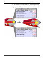
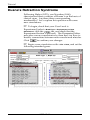
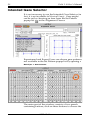
Import Alignment Measurements
Inside the
folder, you will find the
folder. In this folder we have provided
alignment measurements that are the mean of
measurements we collected from 3 cases of left superior
oblique palsy, confirmed by MRI (Demer, et al, 1995)
and with similar surgical treatment:
and
.
We will refer to such data as clinical alignment
measurements, alignment measurements, or just
measurements, the important distinction being between
measurements and simulations. Simulations can predict
measurements, and measurements can test simulations,
but they are not the same.
Orbit measurement files are plain text files, like those
that can be produced by text processor and spreadsheet
programs (these programs must usually be set to
output plain text). Orbit can also save measurements
(and simulated positions) as text files. Details are given
in the Orbit Reference section, below.
1999.09.04
52
Orbit 1.8 User’s Manual
☞ To import pre-operative measurements into Orbit’s
left eye, select » Left Eye » Import Measurements..., which will
lead to a standard Macintosh File Dialog (we show the
new file dialogs, supported by Apple Navigation
Services, incorporated in MacOS 8.5; if you are using an
older operating system, you may see the older style file
dialogs instead). Navigate to the LSO Palsy Example
folder:
☞ Locate and Open the LSO Palsy PreOp LE meas file.
Similarly, select » Right Eye » Import Measurements... to
import LSO Palsy PreOp RE meas into Orbit’s right eye.
1999.09.04
Tutorial
53
We have locked the measurements files to prevent
inadvertent changes, so you will see an alert when you
open them:
Just click
and continue. (We have saved this
stage of the simulation as LSO Palsy PreOp sim (0)).
☞ Bring the Alignment Viewer into the foreground by
clicking or selecting it from the menu bar:
The imported alignment measurements are shown in
red (gray in an achromatic image).
Alignment measurements plotted along with
simulations help evaluate a simulation as it is
developed by trial-and-error. It is also possible to work
on simulations without entering measurements, or use
the alignment chart to display clinical measurements
alone.
1999.09.04
54
Orbit 1.8 User’s Manual
☞
If you wish, you can print the Alignment Viewer
with » File » Print.
☞ You may want to save your own copy of the
simulation as it now stands with » File » Save. We have
locked the measurement and simulation files we
provided, so don’t worry about inadvertently
overwriting them. Create a new folder for your
simulations:
☞ If you are working with Orbit demo (which
disallows saving), simply » File » Quit now, if you want a
break. To resume later without starting over, open
.
1999.09.04
Tutorial
55
Simulate an Abnormality with Live Eyes
One way to create an abnormality is with the Live Eyes
window.
The imported measurements (and, in the present case,
MRI findings) suggest left superior oblique palsy.
That’s where we’ll begin.
☞ Select
» Both Eyes » Live Eyes. The Live Eyes window
will appear. You may need to use the scroll bars and
size box to center the picture.
☞ If the Live Eyes do not look like the figure below,
and choose the Superior point of view.The
click
Live Eyes have 26 regions that produce pop-up
windows when you click on them: the 12 tendons, the
12 muscles, and the 2 globes.
☞ Click once on the left superior oblique muscle:
The muscle Pop-up window allows muscle parameters
to be modified. In a simple SO palsy, contractile
muscle force is 0.
1999.09.04
56
Orbit 1.8 User’s Manual
☞ To simulate simple SO palsy, highlight the
Contractile Muscle Strength box, change it from 100%
to 0, and click
:
If the title bar of the Live Eyes window was visible in
the background, you may have noticed that inverted
and upright question marks (¿ ... ?) appeared around
the simulation name when you altered Contractile
Muscle Strength in the pop-up window. Similarly, the
Alignment Viewer shows the question marks now:
☞ Click on the Alignment Viewer or select
» Both Eyes » Alignment Viewer.
Notice that the question marks disappear when the
Alignment Viewer comes into the foreground. The
question marks indicate that the window is not up to
date. For efficiency, we only update windows when
they are brought into the foreground, eg, by clicking
them. Windows in the background (which are always
dim) may therefore not reflect changes you have
recently made, and the question marks appear to
remind you of this.
1999.09.04
Tutorial
57
We have saved this stage of the simulation as LSO Palsy
PreOp sim (1):
With just one parameter change, the simulation is
already fairly good. The simulated left eye matches the
measurements in showing limited depression,
especially in adduction, and a V-pattern. The tilt of the
arrows, which indicates torsion, shows that simulated
cyclorotation depends on vertical gaze, whereas
measured cyclorotation is less orderly. It is not
unusual to find that measurements of cyclorotation do
not match simulations: this may be because clinical
measurements are often unreliable (Miller and Demer,
1999). In any case, note that the tilt of cyclorotation
arrows in the Alignment Viewer is multiplied by 5 for
visibility, so that most of these discrepancies are small.
Expected secondary deviations are seen in the
simulated following right eye, and these also match the
clinical data.
1999.09.04
58
Orbit 1.8 User’s Manual
The remaining systematic differences are that the
simulation shows greater eso- and left hypophorias,
compared to the measurements. Regarding the left
hypophoria, we suppose that, as a consequence of the
chronically elevated posture of the left eye, the LSR has
shortened by 2 mm (from 32.4 to 30.4). The small
residual horizontal difference between simulation and
measurement is nulled by shortening LLR by 0.7 mm
(from 36.2 to 35.5) and lengthening LMR by 0.7 mm
(from 31.0 to 31.7). We have saved this simulation as
LSO Palsy PreOp sim (2):
In other cases of SO palsy, we might need to consider
additional changes secondary to the palsy, such as: (1)
atrophy of the denervated LSO, that is, subnormal
elastic force, in addition to its absent contractile force,
and (2) adaptation of the cyclovertical muscles which,
chronically held at abnormal lengths, have adapted by
adding or subtracting serial sarcomeres (Tabary, et al,
1972; Williams & Goldspink, 1973), so that their resting
lengths are abnormal.
1999.09.04
Tutorial
59
Plan a Treatment
Now that we have a simulation of the disorder, we can
experiment with treatments.
☞ Open LSO Palsy PreOp sim (2), and import the post-
operative measurements LSO Palsy PstOp LE meas and LSO
Palsy PstOp RE meas. You will by warned about
overwriting the existing pre-operative measurements,
which you want to do. Save the result as
(» File » Save As...) LSO Palsy PstOp sim (0):
Our aim is now to match the simulation to the postoperative measurements.
1999.09.04
60
Orbit 1.8 User’s Manual
Avoid a Poor Treatment
(Note: to follow this section on your computer, you
would need to advance your User Level to Experienced
to gain access to the Mechanical State Viewer (see Orbit
Reference/ Preferences, below). Alternatively, you could
just read this section).
An SO tendon tuck might seem worth a try. Simulation
shows, however, that shortening the LSO tendon by 10
mm corrects hypertropia in up- and level gaze, but
gives little improvement of left eye depression in the
important downgaze reading positions:
Orbit helps understand why this is a consequence of
the SO’s impaired contractility
and normal elasticity.
Before tucking the SO tendon,
we opened » Left Eye »
Mechanical State Viewer, and
choose the most hyperphoric
left eye downgaze position:
Downgaze, particularly in
adduction, is the LSO’s field
of action: its elastic force is
therefore always low, and
here, is near zero. Its
contractile force, because of the paresis is, of course,
zero:
1999.09.04
Tutorial
61
Similarly, we opened the Mechanical State Viewer for
upgaze and adduction (-15, 30), and saw that SO elastic
force was 2.3 g.
Then, we used » Both Eyes » Live Eyes to tuck the SO, by
changing the LSO tendon length from 20.0 mm to 10.0
mm:
Looking again at the Mechanical State Viewers, we
found that downgaze showed only a modest increase in
LSO elastic force to 3.5 g, up from 0.3. This is why the
tuck had little effect in downgaze. In upgaze LSO
elastic force increases substantially to 9.5 g, up from 2.3
g, resulting in a larger corrective effect in upgaze.
Thus, we see that tucking the SO in this case should not
be expected to correct reading positions, and why it
should not. In a different case, the pre-operative
simulation might have included LSO atrophy
(abnormally low elastic force). In such cases, we would
find that an LSO tuck also fails to correct upgaze.
1999.09.04
62
Orbit 1.8 User’s Manual
Plan a Treatment (continued)
These patients actually were treated with RIR recession
of about 4 mm and LIO myectomy or recession.
☞ Here is how to simulate the RIR recession.
Continue from where you imported the post-operative
measurements, or open LSO Palsy PstOp sim (0). Open the
Live Eyes window, choose the Inferior point-of-view,
and click the RIR tendon. The figure of the pop-up
window below shows the Help Balloon, to remind you
that movement “forward” is along a longitude line
from the eye’s posterior pole to its anterior pole, and
movement “around” is along a perpendicular latitude
line:
The Muscle Insertion Movement shown above is 4.1
mm, as reported by the surgeons. But we must also
account for tendon lost during disinsertion and
reinsertion. We estimate that 2 mm are lost, and reduce
RIR tendon length from 5.4 to 3.4 mm.
1999.09.04
Tutorial
63
Compared to postsurgical measurements, the
simulation is still left-hyperphoric, especially in
downgaze (LSO Palsy PstOp sim (1)):
☞ To complete the postsurgical simulation, we need
to simulate the LIO recession performed on these
patients:
1999.09.04
64
Orbit 1.8 User’s Manual
☞ Select » File » Save As... to name this simulation
LSO Palsy PstOp sim(2):
Comparing simulation and post-operative
measurements, we have a good match. The main
discrepancy is the loss of vertical range in adduction.
This is a plausible consequence of weakening both left
obliques, and the mystery is really why clinical
measurements do not show this effect. Further
research would be necessary to determine whether this
is due to central motor adaptation, poor clinical
measurements (eg, incomplete binocular dissociation),
or a problem in the model.
☞ Now, » File » Close Simulation to prepare for a new
simulation.
1999.09.04
Tutorial
65
Lateral Rectus Palsy
This is the simulation that suggested soft rectus muscle
pulleys.
☞ To begin, raise your User Level to Experienced
(select » Both Eyes » Preferences for New Simulations, click the
tab, and select Experienced). This will give you
access to the Parameter Editor, and so, several
parameters not available in the Live Eyes.
☞ Begin a new simulation with
» File » New. Import
the supplied measurements files RLR Palsy PreOp LE meas
and RLR Palsy PreOp RE meas into the left and right eyes,
respectively, and enter some identification:
1999.09.04
66
Orbit 1.8 User’s Manual
☞ Select
» Right Eye » Parameter Editor.
☞ The primary deficit in a complete RLR palsy is, by
definition, the absence of RLR contractility, so set the
RLR Contractile Muscle Strength to 0 (RLR Palsy PreOp sim
(1)):
In the saved file, we set Preferences to suppress alerts
about “solutions not found”. If you did not use this
file, you might see such a message now. It simply
refers to the fact that the paretic right eye could not
fixate all the points we selected, and so corresponding
right eye positions could not be found.
Estimating secondary changes takes some thought –
and some guesswork, since we have only begun to
characterize strabismus syndromes in biomechanical
terms, and to develop ways to estimate parameters in
individual patients (Demer and Kerman, 1994; Demer,
et al, 1994; Demer, et al, 1995; Demer and Miller, 1997;
Demer, et al, 1998; Demer, et al, 1999; Demer and
Miller, 1999):
• We expect atrophy of a chronically paralyzed muscle
(marked reductions in cross-section have been
measured by MRI (Demer and Miller, 1995). Let’s
1999.09.04
Tutorial
67
estimate a 50% reduction in RLR Elastic Muscle
Strength.
• Undoubtedly, the RLR will stretch. We estimate 2
mm of stretch, supposing that the muscle adapts to
the eye’s chronic esotropia.
• There is evidence that modest atrophy occurs in the
antagonist of a paralyzed muscle. We model this by
reducing RMR Contractile Muscle Strength and RMR
Elastic Muscle Strength both to 70% of normal.
• The RMR, too, should adapt to its chronically
reduced path length. We estimate it shortens 2 mm.
• Finally, we know that the antagonist of a chronically
paralyzed muscle may become fibrotic, resisting
elongation beyond what is due to its slight
shortening. This is easily simulated by increasing
RMR Stretch Sensitivity to 125% (see the section
Manipulating the Muscle Model, above).
☞ Using the Right Eye Parameter Editor, make these
secondary changes:
(Note: the unusual “normal” value of 150% for IO
Stretch Sensitivity is an interim solution to the problem
of not yet knowing how to model the IO with
Lockwood’s Ligament. With the usual 100% value, the
IO exerts too little elastic force in downgaze).
1999.09.04
68
Orbit 1.8 User’s Manual
☞ Then activate the Alignment Viewer (RLR Palsy PreOp
sim (2)):
The right eye shows a typical esotropic pattern, with
abduction not reaching the midline. Part of the left eye
pattern is missing because of the paretic right eye’s
restricted range of fixation. Note, however, that the left
eye measurements are more complete than the left eye
simulation. This probably indicates a problem with the
clinical measurements. Consider where the left eye
intends to fix primary position (filled red dot in left
panel above). This measurement should be the position
of the following left eye, where the right eye fixes
primary position. But from the right eye positions in
the right panel, it appears that the right eye cannot get
to primary position. If, by extreme effort, the patient
did get his right eye to primary position, then the
“secondary deviation” of the following left eye would
probably be so large as to put the filled red dot on the
left off the chart. Such subjective alignment measures
as were used to collect these data give no indication of
whether the fixing eye actually achieved the gaze angle
requested, or if the subject just approached it as closely
as he or she could. In the later case, the alignment
measurements are invalid. For this reason, we
disregard the 5 measurements in the rightmost column
for the left eye.
1999.09.04
Tutorial
69
☞ As before, we begin the post-op simulation by
comparing the final pre-op simulation with the post-op
measurements (RLR Palsy PstOp sim (0)):
1999.09.04
70
Orbit 1.8 User’s Manual
We will treat this chronic RLR palsy by transposing the
vertical recti.
Transposition is best performed with the Live Eyes
display, as the directions involved can be confusing*.
With Live Eyes, simply adjust forward and around
values until the picture looks right.
☞ Open Live Eyes and choose the Right Lateral pointof-view:
☞ To remind yourself about directions of insertion
movement, turn on Balloon Help:
*
If you insist on knowing: An advanced insertion moves along the line of muscle pull at
the insertion, in such a direction as to stretch the muscle. A transposed insertion moves in
a direction 90° clockwise from the direction of muscle pull, as viewed from outside the
eye.
1999.09.04
Tutorial
71
☞ Then click the RSR tendon:
☞ Turn Balloon Help off:
1999.09.04
72
Orbit 1.8 User’s Manual
☞ We’re ready to do the RSR and RIR transpositions
(note that we suppose 1 mm of tendon to be lost to the
surgery):
1999.09.04
Tutorial
73
The resulting simulated alignment has the same
“shape” as the measurements, but the simulation is
relatively exotropic, and shows an asymmetry in left
and right eye vertical range that is larger than that
measured (RLR Palsy PstOp sim (1)):
Both of these inconsistencies should be reduced when
we account for stretching of the transposed muscles.
How much are the RSR and RIR stretched?
☞ Open » Right Eye » Mechanical State Viewer and select
primary position (0, 0):
In a normal eye, the superior rectus muscle (SR) and
the inferior rectus muscle (IR) are stretched only 15%,
and we suppose that this represents the target of an
EOM’s length-adaptive processes.
1999.09.04
74
Orbit 1.8 User’s Manual
☞ Use the Right Eye Parameter Editor to increase
RSR Relaxed Muscle Length (mm) from 32.4 to 36.6,
and increase RIR Relaxed Muscle Length (mm) from
34.4 to 39.0. These changes restore RSR and RIR stretch
to 15%. Finally, these patients got some additional
procedures to improve horizontal alignment. We will
simulate the botulinum injection given to one patient
by changing RMR Relative Stretch Sensitivity from 125,
representing “contracture”, to 100%, representing a
muscle that stretches normally.
☞ Finally, to facilitate comparison, we use » Both Eyes
» Gaze Selector to remove from the simulation those
gazes for which we do not have measurements (RLR
Palsy PstOp sim (2)):
The simulation achieves a good match with the clinical
measurements. Some improvement in right eye
horizontal range has been achieved, although not
enough to normalize primary position. As expected,
some vertical range has been lost. The main clinical
problem remaining is the primary position
misalignment, which might have been better managed
by transposing RSR and RIR with posterior sutures
(Foster, 1996).
1999.09.04
Tutorial
75
☞ We can visualize the post-operative eye with
» Right Eye » Graphic Eyes. Here is the right-lateral view
of the right eye, with the left eye fixing (0, 0):
We began by mentioning that this simulation led to the
discovery of soft rectus muscle pulleys. As shown above,
the SR and IR pulleys hold the bellies of the transposed
muscles near their pre-surgical paths.
1999.09.04
76
Orbit 1.8 User’s Manual
What happens without pulleys?
☞ To eliminate pulleys from Orbit 1.8 (thereby
making it behave in this respect like Orbit 1.0) we
locate RSR and RIR pulleys at the muscle origins in the
left eye, right eye and inner eye. (This requires the
Expert User’s Parameter Editor, which shows
coordinates of the muscle origins). Without pulleys,
the transposed muscles take shortest paths, which lie
close to the RLR:
Such muscle paths are not observed in post-operative
magnetic resonance images (Miller, et al, 1993). The
resulting simulated alignment is both alarming and
unphysiologic (RLR Palsy PstOp sim (no puleys)):
The significant difference between the simulations with
and without pulleys is the strangely varying horizontal
misalignment in the later. This occurs because, without
pulleys, the transposed vertical recti acquire actions
similar to the RLR, except they are innervated in upand downgaze.
1999.09.04
Tutorial
77
Duane's Retraction Syndrome
Following Huber (1970), von Noorden (1990)
characterized three varieties of Duane’s on the basis of
clinical signs. Are there three corresponding
mechanisms? Let’s explore this question with some
new simulations.
☞ To begin, check that your User Level is
Experienced (select » Both Eyes » Preferences for New
Simulations, click the
tab, and check that the
Experienced button is pressed). The Parameter Editor
provides a more convenient way than the Live Eyes to
modify connections between motor nuclei and muscles.
Click
to confirm your changes.
☞ Begin a new simulation with » File » New, and set the
following intended gazes:
1999.09.04
78
Orbit 1.8 User’s Manual
Type 1
The descriptive signs of Duane Syndrome Type 1 are:
1. Very limited or absent abduction.
2. Protrusion of globe on attempted abduction.
3. Normal or slightly limited adduction.
4. Globe retraction on adduction.
5. Frequently, up-shoots or down-shoots on adduction.
Signs 1 and 2, and of course the anatomic findings of
Hotchkiss, et al (1980), suggest that the abducens
nucleus is absent or non-functional. Signs 3 and 4
suggest that the MR branch of the oculomotor nucleus
is providing partial innervation to the LR and, so,
producing co-contraction.
☞ Choose » Right Eye » Parameter Editor, and click the
Brain
tab:
The normal connection matrix, above, shows each
muscle fully innervated by “its” motor nucleus or subnucleus (weight of 100%), and not innervated by any of
the other 5 nuclei (weights of 0%). Think of these
connection weights as applied to the motor neurons or
at the neuromuscular junction. That is, nothing about
the fixing eye, or about yoked or antagonistic muscles
is directly changed by changing a connection weight.
Our theory of Duane’s Type I may be expressed as
follows:
1999.09.04
Tutorial
79
Note the “shadows” on the two modified cells. A cell is
shadowed when you modify it (either by typing a new
value or clicking
). Shadows are retained until
you depart from the window, and indicate which
values would be affected by clicking
.
☞ A look at the Alignment Viewer shows that the
rotational defects of Duane’s Type I (signs 1, 3, and 5,
above) are all reflected in the simulation:
Note that up-shoots
and down-shoots
emerge naturally
from co-contraction
in adduction,
essentially in accord
with the theory
advanced by SouzaDias (1976).
Does the pattern of
globe retraction also
fit clinical
expectations?
☞ Select » Right Eye » Mechanical State Viewer, and open
the windows for intended gazes (–40,0), (–20,0), (0,0),
(20,0), and (40,0) -- you can select them all at once by
holding down the key as you click on items in the list
(you’ll need to scroll the window to select them all):
☞ Click
to get a cascade of windows, one for
each fixing eye position, containing values for globe
protrusion under the
tab. As usual, the title
bars of the Mechanical State Viewers are labeled with
the intended gaze position of the following eye, that is,
the position a normal following eye would have gone
to. For example, the intended gaze {40,0} corresponds
to fixing eye gaze {-40,0}, because when the fixing eye
adducts (negative) the following eye abducts (positive).
1999.09.04
80
Orbit 1.8 User’s Manual
The title of this window indicates that a normal
following eye would have been 40° in abduction (40,0),
and gives the values for the sick following eye: it’s
highly eso- and slightly hyper-deviated, and shows 0.3
mm of globe retraction.
A reasonable way to evaluate globe translation is in
comparison to the normal eye:
Intended
Horizontal
Gaze
Normal Eye
Protrusion
Duane’s I Eye
Protrusion
Duane’s I
Relative
Protrusion
-40
-20
0
20
40
-0.7
-0.5
-0.5
-0.6
-0.9
-1.3
-0.8
-0.4
-0.3
-0.3
-0.6
-0.3
+0.1
+0.3
+0.6
So, with respect to globe translation, our simulation
predicts the expected pattern: retraction (negative
protrusion) in adduction and protrusion in attempted
abduction. However, the total range of abnormal axial
translation, just over 1 mm, seems a bit small. Should
you wish to pursue this simulation further, you might
advance to Expert Level, which allows you to modify
Globe Translational Stiffness. We think it reasonable to
guess that a chronic co-contractive syndrome would
soften the encapsulated fat pads that control globe
translation. Reducing Globe Translational Stiffness
greatly increases the magnitudes of retraction and
protrusion.
Type 2
The signs of Duane’s Type 2 are:
1. Normal or slightly limited abduction
2. Limited or absent adduction
3. Globe retraction on attempted adduction
4. Frequently, up-shoots or down-shoots on adduction
Our theory is that abducens innervation of LR is
normal (sign 1), but that the MR branch of the
oculomotor nucleus is providing partial innervation of
LR (signs 2, 3 and 4). One change to the Connection
Matrix ...
1999.09.04
Tutorial
81
... results in the
following Alignment
Chart:
Type 3
Duane’s Type 3 is characterized by:
1. Limited or absent abduction
2. Limited or absent adduction
3. Globe retraction on attempted adduction
4. Frequently, up-shoots or down-shoots on adduction
We leave this simulation as an exercise for the reader.
1999.09.04
82
Orbit 1.8 User’s Manual
1999.09.04
Orbit Reference
83
Orbit Reference
Here, following some general comments on Orbit
windows, we provide complete descriptions of each.
Two Types of Windows
Does the window have an
button? If so, you
must finish your work there and close it before doing
anything else.
Most windows, however, don’t have
buttons,
and it is convenient to leave several of them open on
your desktop. We leave open Live Eyes or Parameter
Editor (for trying different lesions and procedures),
Alignment Viewer (to see the overall results), and
Mechanical State Viewer (for corresponding numeric
values).
Orbit windows (except the Parameter Fitter) know
about each other: if you make a change (eg, with the
Parameter Editor), all dependent windows (eg, the
Alignment Viewer & Mechanical State Viewer) will
know that they are out of date. For efficiency, however,
we do not update background (ie, dim) windows until
they are brought into the foreground. To remind you
that the values in a background window may not be
current, inverted and upright question marks (¿ ... ?)
are placed around the simulation name. If you select
an out of date window (eg, by clicking it to bring it into
the foreground) it will update, and the question marks
will disappear.
1999.09.04
84
Orbit 1.8 User’s Manual
Preferences
There are three types of settings with which you can
customize the behavior and appearance of Orbit and
simulations you create. They differ in “scope”:
•
can be set to customize
subsequently created, new simulations. These
preferences are saved in the file Orbit_Prefs, which is
associated with the Orbit application. Thus, these
preferences remain in effect for a given copy of
Orbit, until you change them (or trash the
Orbit_Prefs file).
•
Preferences for Active Sim sim_name contains
Preferences for New Simulations
many of the
same settings, but only affects the currently active
simulation. These preferences are saved are saved in
the simulation file, and, so, re-assert themselves only
when that simulation is opened.
• Finally, several windows offer Window Settings
buttons,
, which can be used to quickly and
temporarily override the preferences for that
window only. These are described in connection
with individual windows.
The Preferences window » Both Eyes » Preferences for New
Simulations) lets you to customize simulations that you
subsequently create (using » File » New). The
Preferences window » Both Eyes » Preferences for Active Sim
sim_name lets you customize the simulation that is
currently active. The contents of the two preferences
windows are similar.
Offers this explanatory page.
Returns all preferences to factory settings.
Closes the preferences window, ignoring any
changes you might have made.
Accepts settings and closes the window.
Settings are divided into groups, each group attached
to
.
1999.09.04
Orbit Reference
85
The General preferences tab appears only in Preferences for
New Simulations. General preferences are settings not
specific to any single simulation or window:
These check-boxes determine what
happens when the program is launched by doubleclicking on the Orbit icon. It seems reasonable to begin
a new Normal Eyes simulation, since if you had
wanted to begin with a particular existing simulation,
you could have double-clicked on that simulation. A
new user will benefit from having the What is Orbit™?
window open, but will soon want to deselect it.
Open on Orbit Launch.
allows you to create
simulations based on alternative normal eyes that you
create. (Sorry, not implemented in version 1.8).
Choose Normal Eye Description
Intended Gaze Selector
sets the gaze angles in a new
simulation.
1999.09.04
86
Orbit 1.8 User’s Manual
All other tabs appear in both preferences windows.
The Sim tab contains preferences that apply to an entire
simulation:
At lower User Levels, options are limited, to
highlight basic operations. Novice users are not offered
certain windows at all (they are dimmed in the Menu
Bar); others appear in simplified form. Experienced
users are offered all windows, but three of them, the
Measured Gaze Editor, Mechanical State Viewer, and
Eye Parameter Editor, appear in simplified forms.
Almost all users of Orbit will begin at the Novice, and
then advance to the Experienced level. (It is not
allowed to lower the User Level of an existing
simulation, because this could make inaccessible some
values previously modified).
User Level.
Have the windows you always use
open automatically. On a slow machine it may take
significant time to open large or graphic windows, and
windows that require the simulation to update.
Open with Simulation.
This will
appropriately change the deviation values shown in
various windows and their unit labels.
Show gaze angle differences in prism diopters.
can be checked if
you don’t wish to be notified when one or more gaze
angles fail to converge.
Suppress alerts about solutions not found
1999.09.04
Orbit Reference
87
The AlignVu tab contains preferences for the Alignment
Viewer window (» Both Eyes » Alignment Viewer):
Near the top of the Alignment Viewer is a HessLancaster-type Alignment Chart, which always shows
intended gazes (+), and optionally shows simulated
positions of the following eye (blue o), and
measurements (red o).
Below the Alignment Chart is the “tic-tac-toe”
Deviation Chart. Deviations are differences between
actual and intended gaze positions. Choose whether to
view simulated deviations of the following eye, or
measured deviations. Choose which deviations to
show, by their intended gaze. If you have not selected
some chosen positions with the Intended Gaze Selector,
the chart will show blank boxes.
The Param Fit tab contains preferences for the Parameter
Fitter window (» Both Eyes » Parameter Fitter) that allow you
to modify the fitting method:
Choose the Mean Error Criterion if you want the best
overall fit across all gaze positions for which
measurements have been entered (this might allow a
few badly fitted positions, but is usually the best
choice). Choose the Maximum Error Criterion if you
want the worst fitted position to be as good as possible.
are values from 0 to 10 which determine the
relative (ie: 1,1,1 is the same as 10,10,10) significance of
Weights
1999.09.04
88
Orbit 1.8 User’s Manual
each gaze angle component in the fitting algorithm. A
weight of 0 means that the component is ignored in
calculating the error that is minimized. Thus, because
torsion measurements can be unreliable, its weight is
often set to 0. If the torsion component is omitted from
a measured gaze point it is, of course, omitted
regardless of the weight.
It is possible for the Parameter Fitter to try eye
parameters that Orbit cannot solve for some gaze
angles. This may mean parameters are unrealistic,
measurements are inaccurate (or Orbit is flawed). You
may wish to allow a small number of Convergence Failures
so that you can proceed.
Set Beep when done to be prompted when a fit is
achieved. Fitting will take longer if you choose
parameters from both eyes, many parameters, or many
gaze angles.
The Graph Ey tab contains preferences for the Graphic Eyes
window:
Show.
The structures selected are shown.
The saturation (purity) of the red muscle
color is an index of the chosen Variable. Pure red
indicates the value you enter in Maximum Saturation,
and gray, the value in Minimum Saturation.
Muscle Color.
Choose to write each Graphic Eyes window
produced as a “PICT” type file in the folder specified.
Orbit movies are made using a sequence of such PICT
files. Note that if you leave this box checked
unintentionally, you will create many unwanted PICT
files!
Files.
1999.09.04
Orbit Reference
89
Checking Beautify increases the resolution of the
drawing.
The LiveEy tab contains preferences for the Live Eyes
window:
Show.
The structures selected are shown.
1999.09.04
90
Orbit 1.8 User’s Manual
Intended Gaze Selector
It is not necessary to use the Intended Gaze Selector (in
fact, it is not available to Novice Users). Gaze angles
can be set by choosing an item from the Set Pattern
popup list
in the Alignment Viewer:
Experienced and Expert Users can choose gaze patterns
not available in the Set Pattern popup list by opening »
Both Eyes » Gaze Selector:
The main part of the window consists of two panels
containing buttons; click on these buttons to choose the
1999.09.04
Orbit Reference
91
gaze angles to which each simulated eye attempts to
rotate (moving “under cover”).
Intended gaze positions of the left eye are chosen on
the left, and those of the right eye on the right,
following the perspective of the Alignment Chart.
Abducting and adducting directions are as labeled near
the top of each panel (the nose is between the two
panels). All angles are in degrees.
Consider, eg, the gaze position for which the right eye
will attempt to abduct 30° and elevate 30°. In terms of
the Hess-Lancaster test, this means that the patient will
be instructed to adduct 30° and elevate 30° with the
fixing left eye. If both eyes are normal, the following
right eye will go to the intended positions exactly.
Otherwise, it may go somewhere else.
Remember that to Import clinical measurements (» Left
Eye » Import Measurements or » Right Eye » Import
Measurements), the intended gaze angles must already be
in the simulation, eg, chosen in the Intended Gaze
Selector.
1999.09.04
92
Orbit 1.8 User’s Manual
Alignment Viewer
Use the Alignment Viewer to view simulation results
and measurements.
Info Fields
The top part provides fields to record patient and
simulation information, and shows the alignment chart.
Help balloons (» Help » Show Balloons) associated with the
patient and simulation information fields suggest how
these fields may best be used.
Alignment Chart
Below the information fields is a Hess-Lancaster-type
alignment chart. The orientation of the chart follows
clinical convention, with positions of the following (ie,
“moving under cover”) left eye on the left, and that of
the following right eye on the right.
Each intended gaze position is represented as a small
black cross, “+”. The intended gaze position of a
following eye is the position it would assume if the
1999.09.04
Orbit Reference
93
whole system were normal. Equivalently, it is the
position of the fixing eye, with the signs of horizontal
and torsional gaze components reversed (because of the
eyes’ mirror symmetry). The set of intended gaze
positions for each eye can be selected from pop-up lists
above the alignment charts:
Positions of the following eye are shown as blue circles,
“o”, with connecting lines to emphasize the pattern.
An arrow through each circle shows cyclorotation
(torsion in excess of normal Listing’s Law torsion), as
tilt from straight up, multiplied by 5 for visibility. Any
clinical alignment measurements you have entered are
shown as red circles, “o”, with red connecting lines.
All angles are in degrees.
Window Settings & Help
At the top of the window are a window settings button
, and a window help button
. The window
help button, you will recall, provides the present
description.
Pressing
gives:
Here, we’ve chosen both simulation results and clinical
measurements to appear in the alignment chart (as
shown above).
1999.09.04
94
Orbit 1.8 User’s Manual
We have also chosen to show deviations (from
intended gazes) of the simulation results for ±30°
intended gazes (primary position is always shown, as
well).
To apply these settings and return to the Alignment
Viewer, press
. The new settings are temporary,
in that they are associated with the current instance of
the Alignment Viewer window; if you close and then
reopen the Alignment Viewer, settings will revert to
those given in » Both Eyes » Preferences for Sim.... Clicking
has the same effect. Press
to
undo any changes.
Deviation Chart & Notes Box
Scrolling or enlarging the Alignment Viewer reveals
the deviation chart and the notes box. Each panel of the
deviation chart shows the same information as the
panel of the alignment chart above it, except in a
different (numerical) form:
A deviation is a difference between following and
intended gazes: positive values of exo mean the
following eye is excessively abducted, hyper means it
points too high, and excyclo means it is excessively
cyclorotated such that the top of the eye has turned
laterally. Labels on the right tell whether deviation
units are deg or prism diopters (this is set in » Both Eyes
» Preferences).
Use the notes box as you wish. We use it to document
the simulation.
1999.09.04
Orbit Reference
95
Live Eyes
The Live Eyes window provides simplified access to
the most frequently used eye parameters, the only
access available to Novice Users. Experienced and
advanced users may prefer it to the Parameter Editor
for operations like transposing an insertion, since the
Live Eyes will show you if you moved in the desired
direction. Also, you see immediately if the eyes
responded to your manipulation as expected. If
manipulations are confined to one muscle or tendon, it
is easier to find the correct parameter with Live Eyes.
On the other hand, if you’re working with several
muscles, the Parameter Editor will be more convenient.
The Live Eyes have 26 regions that produce “pop-up
windows” when you click them. These regions are: the
12 tendons, the 12 muscles, and the 2 globes. A desired
region can be made visible by changing Point of View
or by using the windows settings button
to hide
occluding structures.
In simulating resection surgery, you may reduce a Live
Eyes tendon length to zero, and then be surprised to
find that a length of tendon is still shown. This is
intentional, since, if a tendon disappeared, its pop-up
window would become inaccessible.
Clicking the windows settings button
allows
you to choose which structures are shown. You can
adopt previously set simulation preferences as current
window settings with
. Apply your
choices to the current Live Eyes window by clicking
.
, or forget them by clicking
1999.09.04
96
Orbit 1.8 User’s Manual
Live Eyes are drawn with Left Eye and Right Eye
parameters, driven by Normal primary position
innervations. This allows the Live Eyes to be drawn,
regardless of parameter values. Consequently, the Live
Eye will now show abnormalities intrinsic to an eye,
but not abnormalities mediated by abnormal
innervations (eg, “secondary deviations”). Graphic
Eyes, of course, show all abnormalities, where solutions
can be found.
Live Eyes uses color to determine the structure clicked.
If it is not responding properly, your Macintosh color
table may have been altered. Graphics applications
sometimes alter the color table, and are supposed to
restore it when they quit or are put in the background,
but not all do. Quitting the offending program usually
solves the problem.
1999.09.04
Orbit Reference
97
Parameter Editor
The Parameter Editor provides Expert Users access to
all Orbit parameters, and Experienced Users access to
all but some seldom-used parameters. (Novice users
are restricted to the frequently used variables given in
Live Eyes pop-up windows).
Extensive Balloon Help (» Help » Show Balloons) defines
all parameters and other terms used in the Parameter
Editor.
Parameter values are changed in the usual way, by
selecting and editing. All non-normal values appear in
red. Values altered during the current visit to the
Parameter Editor are additionally marked with a red
drop-shadow. Click
to restore these parameters
to the values they had when you last left the Parameter
Editor. The
button sets all parameters to
normal eye values. The Normal field (in the upper
right corner of the window) shows the normal value of
the selected parameter.
Exporting Eye Parameters
The eye parameters available in the Expert Level
Parameter Editor can also be saved to a text file for use
with another application, such as a text editor or
spreadsheet, with » Left Eye » Export Eye Parameters and
» Right Eye » Export Eye Parameters.
1999.09.04
98
Orbit 1.8 User’s Manual
Parameter Fitter
The Parameter Fitter allows Experienced and Expert
Users to automatically optimize the fit of an Orbit
simulation to a set of clinical measurements by varying
selected eye parameters. It uses the Nelder-Mead
Simplex algorithm (Press et al, 1992, Numerical Recipes
in C: The Art of Scientific Computing, edn 2).
Open » Both Eyes » Parameter Fitter and the Parameter
Editor(s) for the parameters you wish to vary. Select
each parameter (drag across it, highlighting the entire
field), and then drag and drop it into the lower part of
the Parameter Fitter window. The parameter will
expand into a line showing the eye, muscle, parameter
name, initial value taken by the fitting procedure,
minimum and maximum values, and the value arrived
at by the fitting procedure:
is “L” for left eye, “R” for right eye, or “3” for third,
inner eye (the Inner Eye is briefly described above, in
the Test of Binocular Alignment section).
Eye
Mus
is “LR”, “MR”, “SR”, “IR”, “SO” or “IO”.
is the parameter name, as in the Parameter
Editor, possibly abbreviated.
Parameter
is the initial value taken by the fitting procedure.
It is set to the current value by default. If you have a
better guess, enter it, since it is best to begin fitting with
eye parameters close to those desired. The less distance
in parameter space the algorithm has to traverse, the
less likely it is to get trapped in a local minimum and
quit with unsatisfactory parameters.
Initial
and Max are lower and upper limits on parameter
values the Fitter will try. They are empty by default,
meaning no limits. If the Fitter wanders into
implausible values, constrain it by setting these limits.
The alert “The biomechanical model could not handle
the eye parameters...” means that the fitter has tried
frankly illegal values (such as a negative muscle length
or strength). You can dismiss the alert and fitting will
continue. It might be better to set Min and Max values
to keep the fitter out of trouble. A parameter’s initial
value will be forced to lie between the two limits.
Min
The Fit field shows the parameter value arrived at by
the fitting procedure. While the Fitter is running it
1999.09.04
Orbit Reference
99
shows the values tried. When the Fitter is done it
shows the best value found.
The Help button shows information similar to this
Manual section.
The Settings button opens a window in which you can
modify the fitting method:
Choose the Mean Error Criterion if you want the best
overall fit across all gaze positions for which
measurements have been entered (this might allow a
few badly fitted positions). Choose the Maximum
Error Criterion if you want the worst fitted position to
be as good as possible.
are values from 0 to 10 which determine the
relative (ie: 1,1,1 is the same as 10,10,10) significance of
each gaze angle component in the fitting algorithm. A
weight of 0 means that the component is ignored in
calculating the error that is minimized. Thus, because
torsion measurements can be unreliable, its weight is
set to 0 by default. If the torsion component is omitted
from a measured gaze point it is, of course, omitted
regardless of the weight.
Weights
1999.09.04
100
Orbit 1.8 User’s Manual
It is possible for the Parameter Fitter to try eye
parameters that Orbit cannot solve for some gaze
angles. This may mean parameters are unrealistic,
measurements are inaccurate, or Orbit is flawed. You
may wish to allow a small number of such Convergence
Failures.
Set Beep when done to be alerted when a fit is achieved.
Click
to accept the settings shown for the current
simulation and return to the Parameter Fitter,
to
abandon any changes and return, or
to make the window show the values from Preferences.
The
button starts the parameter fitting
algorithm. The “wait cursor” will show that Orbit is
busy. As the fitter works it will show:
Iteration
– the number of parameter sets tried.
(or Initial Maximum Error) – the fitting error
for the initial parameter values. A special error value
of 9999.99 means that, with the initial parameters,
solutions could not be found at more points than
allowed by the Convergence Failures Allowed setting.
Either pick better initial parameter values, or allow
more convergence failures.
Initial Mean Error
(or Current Maximum Error) – the fitting
error for the current parameter values. This field
updates as the algorithm works. The 9999.99 error
value, meaning excessive convergence failures, is
normal during fitting -- the procedure will back away
from the troublesome parameter value and try
something else.
Current Mean Error
Watch the Iteration, Current Error and Fit value fields to
judge the algorithm’s progress. If it seems to be going
wrong (unbelievable parameter values), or nowhere
(stuck in a “local minimum”), hold down both the
and . keys until the algorithm stops.
takes corresponding values from the
simulation and makes them the initial values for the
fitting algorithm. This may be useful if, since initially
dragging parameters to the Parameter Fitter, the
simulation has been updated (eg, by previously
Applying fitted values).
places the fitted values into the simulation. It
can be used when the fitting procedure finishes, or
when it is stopped with . .
1999.09.04
Orbit Reference
101
A multidimensional fitting routine is not guaranteed to
work in every case. Some tips:
• Be sure the Fitter can get started. If Initial Error is
9999.99, one or more gaze positions cannot be
solved for the initial parameters. Change an initial
parameter, or look at the Alignment Viewer to
find the gazes at fault. Then, either allow for that
number of Convergence Failures, or remove the
troublesome positions with the Intended Gaze
Editor.
• It will usually improve the fit to re-run the Fitter
after it claims to have found a minimum. Thus,
after fitting you might click Apply, Load Initial,
and Fit, to start a new search from the previously
found parameters.
• You must always ask yourself: Do these parameter
values make sense?
To fit n parameters, the Nelder-Mead Simplex
algorithm works in an n-dimensional space with n+1
points (eg, a triangle for n=2, a simplex in general)
which might contain the sought-for minimum. On
each iteration it varies one or more parameters to learn
about the local terrain, and when it has varied all
parameters, guesses a new (n-dimensional) position for
the worst fit point and calculates the new error. When
the simplex encloses a point of relative minimum error,
it tends to shrink, and when it’s small enough, the
algorithm quits.
Thus, during terrain mapping, parameter values and
Current Error will normally change and then change back.
A new n-dimensional guess may increase Current Error,
because it reflects the worst of three points (ndimensional parameter sets), and because of poor
guesses.
1999.09.04
102
Orbit 1.8 User’s Manual
Measured Gaze Editor
In the SO palsy simulation, above, we imported a file of
clinical measurements. It is also possible to enter
clinical measurements individually from the keyboard.
To do so, select » Right Eye » Measured Gaze Editor, and
choose all gaze positions for which you have data (use
shift-click to select contiguous multiple items or
command-click to select disjoint multiple items), and
click
.
Title bars of the Measured Gaze Editors, like those of
Mechanical State Viewers are labeled with the intended
gaze position of the following eye, that is, the position a
normal following eye would have gone to. (For
example, intended gaze (-30,30) corresponds to fixing
eye gaze (30,30), because when the fixing eye abducts
(positive) the following eye adducts (negative). If a
cyclorotation is unknown, leave the excyclo-rot field
blank (not 0).
The Expert Level Measured Gaze Editor also contains
fields for eye translation, in the unlikely event that they
are actually measured.
1999.09.04
Orbit Reference
103
Importing Clinical Measurements
Many clinicians enter alignment measurements into
spreadsheet or database programs. Most such
programs can write their data as "tab-separated text", or
some similar file format intended for export to other
programs. Orbit can read most such files directly.
Each line in an imported file can contain the following
values, in order, separated by tabs, spaces, or commas:
1. intended abduction (deg)
2. intended elevation (deg)
3. measured abduction (deg)
4. measured elevation (deg)
5. measured excyclorotation(deg)
6. measured sideways globe translation (mm)
7. measured protruding globe translation (mm)
8. measured upward globe translation (mm)
The first two fields identify each line by horizontal and
vertical intended gaze positions; the remaining values
are optional. If a value is unavailable, use 999 as a
placeholder. It's also OK to have "short" lines, which
omit trailing values (eg: globe translation and extorsion
are rarely measured, so the last 3 values will usually be
omitted).
So that it can read files that contain other text besides
the data, Orbit ignores: lines beginning with the
following three characters: # ; > (so, these characters
can be used to introduce comment lines), tabs and
spaces at the beginning of a line (allowing indentation),
and all characters that are not digits, +, -, or . (so,
numbers must not be expressed in scientific or
engineering notation).
Recall that excyclorotation, as in field 5, is abnormal
extorsion, extorsion beyond that expected from
Listing’s Law. For eyes that obey Listing’s Law (eg,
normal eyes), excyclorotation will always be zero.
1999.09.04
104
Orbit 1.8 User’s Manual
Here is an example of a valid import file:
#
#
#
#
#
#
#
Generic LR Palsy PreOp
measurements for
Orbit™ 1.8 tutorial
Intended
Ad
Up
-30
-30
-30
-15
-15
-15
-15
-15
0
0
0
0
0
15
15
15
15
15
30
30
30
-15
0
15
-30
-15
0
15
30
-30
-15
0
15
30
-30
-15
0
15
30
-15
0
15
Following Eye
Ab Up Excy
-37
-37
-38
-27
-26
-25
-26
-26
-17
-16
-16
-17
-16
-11
-9
-10
-10
-10
-8
-8
-9
-14
0
13
-28
-14
0
13
27
-29
-15
0
14
28
-30
-16
0
14
28
-17
-1
15
1999.09.04
0
0
0
0
0
0
0
0
0
0
0
0
0
0
0
0
0
0
0
0
0
Orbit Reference
105
Exporting Measurements & Simulated
positions
If you have imported clinical measurements, or entered
or modified clinical measurements using the Measured
Gaze Editor you may want to write them to a text file
for use with another application, such as a text editor or
spreadsheet. To write measurements to a file use » Left
E y e » Export Measurements or » Right Eye » Export
Measurements.
It may also be useful to write simulated gaze positions
to a text file. Use » Left Eye » Export Simulation or » Right
Eye » Export Simulation.
(Orbit demo cannot export measurements or simulated
gaze positions.)
1.
2.
intended abduction (deg)
intended elevation (deg)
3.
4.
5.
measured or simulated abduction (deg)
measured or simulated elevation (deg)
measured or simulated excyclorotation(deg)
6. measured or simulated sideways globe translation
(mm)
7. measured or simulated protruding globe translation
(mm)
8. measured or simulated upward globe translation (mm)
9.
measured or simulated extorsion (deg)
Export formats are similar to import formats (see
above), with the addition of a 9th field on each line.
Measured or simulated extorsion is included for the
convenience of workers who need the 3rd Fick
coordinate of measured or simulated gaze. You will
recall that Field 5, excyclorotation, is not the torsion
value that goes with abduction and elevation – it is
abnormal torsion. Thus:
excyclorotation = extorsion – normal_extorsion
where normal_extorsion follows Listing’s Law.
Clinicians, we think, will usually be interested in
excyclorotation, and scientists in extorsion.
1999.09.04
106
Orbit 1.8 User’s Manual
Mechanical State Viewer
The Mechanical State Viewer shows rotations,
deviations, innervations, forces, and other variables,
determined by simulation for a given gaze position. (In
contrast, the Parameter Editor is used to view and edit
parameters, values that characterize an eye and are
constant across gaze positions.) The title bar of the
Mechanical State Viewer shows the simulation name
and the intended gaze position. Expert Users are
shown all Orbit variables; Experienced Users are
shown a reduced set. (Novice users are restricted to the
eye position information in the Alignment Viewer).
The title bars of Mechanical State Viewers are labeled
with the intended gaze position of the following eye, the
eye whose variables it shows. The intended gaze
position is the gaze position a normal following eye
would have adopted for the corresponding fixing eye
position.
Extensive Balloon Help (» H e l p » S h o w B a l l o o n s ) defines
all variables and other terms used in the Mechanical
State Viewer. Variables in the Muscle Forces Tab
require some additional explanation.
Muscle Forces
The Muscle Forces Tab in the Expert Level Mechanical
State Viewer is used to answer questions such as these:
• How much force does each muscle contribute to
eye rotation (as contrasted with eye translation)?
• What is the axis, in Cartesian head-relative
coordinates, about which a muscle rotates the eye?
Researchers interested in how the brain controls
eye movement need to know this instantaneous
velocity axis.
• How does each muscle contribute to abduction,
elevation, and extorsion? These three rotations,
describe the Fick coordinate system (discussed
above), familiar to clinicians.
• Has a muscle lost tangency with the globe? Is it
now expending force in globe translation, at the
cost of globe rotation?
1999.09.04
Orbit Reference
107
• What is the total longitudinal tension in the
muscle, and how much of it is due to contractile,
elastic, and constant (eg, externally applied)
forces.
• What forces do the muscles exert due to their
sideways bending?
T o ta l L o n g itu d in a l Mu s c le F o r c e (g )
Total Longitudinal Muscle Force is the total force
exerted by a muscle along its length, that is, in the
direction of its fibers. We conceive of it as the sum of
three component forces: Contractile Force, Elastic
Force, and Constant Force, as described above (see
section: Muscle Force Model).
1999.09.04
108
Orbit 1.8 User’s Manual
R o ta tio n a l Mu s c le F o r c e (g )
Rotational Muscle Force is the vector sum of moments
due to the Total Longitudinal Muscle Force and the
Rotational Force Due To Muscle Width. Both
component moments reflect the local globe radius and
Moment Arm Factor.
So long as a muscle remains tangent to the globe, it will
pull perpendicular to the globe radius, and exert all of
its force (Moment Arm Factor = 100%) in rotating the
eye. If the muscle looses tangency with the globe
(Moment Arm Factor < 100%), Rotational Muscle Force
is proportionally reduced.
1999.09.04
Orbit Reference
109
U n it Mo m e n t V e c to r (% )
The Unit Moment Vector (conventionally symbolized
as m), describes the axis about which a given muscle
tends to rotate the eye. m is described in a Cartesian
coordinate system fixed to the orbital bone (see the
figure below).
The components of m are shown in the figure as mx,
my and mz. The “spin” arrows show the rotations
associated with positive values of each component: mx
= up, my = out, mz = medial (it would not have been
correct to reuse the terms elevate, extort, and adduct,
because they refer to components in the rotating Fick
coordinate system).
mx, my and mz are orthogonal vector components, so
that the square root of the sum of their squares equals
one, or 100%.
R o ta tio n a l F o r c e c o m p o n e n t (g )
Strabismus surgeons, who think about eye rotations in
terms of the conventional Fick coordinate directions of
abduction, elevation and excyclorotation, wish to know
how the Total Rotational Force of a muscle acts in each
direction. We call these values Rotational Force
Components.
1999.09.04
110
Orbit 1.8 User’s Manual
Unlike the Unit Moment Vector, Rotational Force
Components are not defined in a fixed, orthogonal
coordinate system: they are defined in the nonorthogonal, rotating Fick coordinate system described
earlier. In consequence, abducting, elevating and
excyclorotating components will not necessarily sum as
vector components. Indeed component forces may be
larger than the Total Rotational Muscle Force! (If this
seems strange, consider the game “tug of war”, in
which two very large, opposing component forces yield
a near zero resultant).
Regardless of how the eye arrived there, a given
rotated position is specified in Fick coordinates as
though the eye started in primary position, and then
rotated as follows. First, the eye is imagined to rotate
in abduction or adduction about the earth-vertical axis
z. Second, it rotates in elevation or depression about x’,
a new axis, which was not defined prior to the rotation
about z. The axis x’ is derived from the axis x, rotated
1999.09.04
Orbit Reference
111
with the eye about z. Finally, cyclorotation – rotation
about the visual axis – is defined about y’’, which axis
has rotated with the eye through the two preceding
rotations.
Exporting Mechanical States
The mechanical state variables available in the Expert
Level Mechanical State Viewer can also be saved to a
text file for use with another application, such as a text
editor or spreadsheet, with » Left Eye » Export Mechanical
State and » Right Eye » Export Mechanical State.
1999.09.04
112
Orbit 1.8 User’s Manual
Point of View
The Live Eyes and Graphic Eyes displays represent 3dimensional objects on a 2-dimensional surface. To
adjust how they are viewed, use » Both Eyes » Point of
View. Novice-level users get a simplified POV Editor
that allows them to select from among named points of
view. Experienced and Expert Users get the complete
POV Editor, which allows them to create arbitrary
POVs and name them for future use with the
button. Named POVs can be deleted with
.
To use the complete POV Editor, imagine you are
setting up a camera to take a picture of a 3-D object,
and that the picture is the size of your Macintosh
screen. Enter values of Field, Roll, View From, and Look
To, using either the scroll bars or the numeric boxes.
Field is the angular extent represented in the picture.
View From is the point at which you set the camera; Look
To is where you point it. Roll is rotation of the camera
around the viewing axis (the line joining View From and
Look To).
Press
to see a normal eye fixing primary
position, as it would appear from the current POV.
When satisfied, click
. Existing and new Live
Eyes and Graphic Eyes will be shown from the new
POV.
1999.09.04
Orbit Reference
113
Graphic Eyes
Graphic Eyes produces a high-resolution picture of
following and fixing eyes in any of the gaze positions
previously selected with the Intended Gaze Selector
(the Live Eyes display shows only primary position, its
main purpose being access to eye parameters). Muscles
are shown in red, with saturation related to one of
several model variables. Select » Left Eye » Graphic Eyes
for a representation in which the left eye is following
and the right eye fixing, or » Right Eye » Graphic Eyes for
the reverse.
The window settings button
following options:
provides the
The two groups of 7 check boxes let you chose which
structures are shown. Below them is a popup list of
variables than can be represented by muscle color.
Choose: total muscle force (in grams), contractile muscle
force (in grams), elastic muscle force (in grams), stretch (in
mm, relative to relaxed length), stretch (as percent
change from relaxed length), or innervation (in arbitrary
units). Then set the values to be associated with
minimum (gray) and maximum (pure red) muscle color
saturation.
1999.09.04
114
Orbit 1.8 User’s Manual
If you wish to save Graphic Eyes pictures to disk (eg,
for printing), check Write PICTs. PICT files are graphics
files, readable by most graphics applications. Press
to determine where the files will be saved.
Beautify increases the resolution of the pictures (which
consequently, take longer to draw). Having checked
Write PICTs, each time you create or alter a Graphic Eyes
window, a PICT file will be written to the chosen
folder, its name derived from the Graphic Eyes
window title bar. Remember to uncheck Write PICTs
when you’re done saving PICTs since, otherwise,
unwanted files will accumulate.
Click
to adopt as current window
settings the values saved in » Both Eyes » Preferences for
to apply your choices to the current
Sim... Click
Live Eyes window, or
to forget them.
1999.09.04
Orbit Reference
115
Other Issues
Names
The title bar of most Orbit windows gives the name of
the simulation (eg: untitled). If the window pertains to
a particular intended gaze position, it too is shown in
the title bar (eg: untitled/0,0).
Speed
Hardware: The hardware on which you run Orbit is
the most important determinant of speed.
For comparison, we ran a simulation with normal eyes
and all 289 gaze angles for one eye. All calculations
shown in the flowchart shown in the section Test of
Binocular Alignment were run by manipulating
parameters in both left and right eyes.
Quadra 700
740 sec
-----------------------------PowerMac 6100/60
140
iMac G3/266
20
PowerBook G3/292
15
PowerMac G3/300
15
Machines with the PowerPC RISC processor (below the
line) are much faster than the 680X0-based machines
they replaced (above). This is because Orbit spends
most of its time doing “floating point” calculations,
which are a special strength of the PowerPC. Speeds
for the G3 and G4 (types of PowerPCs) should vary
with processor speed.
If you have a slow machine, buy enough memory so
you don’t have to use Virtual Memory. Turn off File
Sharing. (See your Macintosh Owner’s Manual for
information about Virtual Memory and File Sharing).
System Software: Some INITs (software placed in the
Control Panels or Extensions folders of the System
Folder) can slow your Macintosh down.
Experimentation can tell you if a particular INIT (or a
particular combination of INITs) is exacting too high a
cost. Create folders like
1999.09.04
and
116
Orbit 1.8 User’s Manual
, and drag any offending INITs to them.
Restart your Macintosh to run without the disabled
INITs. Move them back and Restart to re-enable them.
Programs called extension managers provide an
equivalent, more convenient way, to enable and disable
INITs.
Use of Orbit: If you do not have a fast machine, you
will not want to use the Parameter Fitter.
Calculations are much simpler and faster if the fixing
eye is normal. With a slow computer, try to work with
only one abnormal eye, and to have that eye be the
following eye only. That is, do not simulate
“secondary” deviations.
Windows like the Parameter Editor and the Mechanical
State Viewer may take a moment to open, because of
the large number of fields they contain (particularly at
Expert level). But there is no need to close them and reopen them for each use -- just leave them open.
The time it takes for the biomechanical model to run is
proportional to the number of fixation points chosen.
Use the Intended Gaze Selector to reduce the number of
gaze positions to the minimum needed.
Printing
You can print Orbit windows to record patient data,
intermediate simulation stages, or simulation results.
We find it most useful to print the Alignment Viewer,
which contains patient and simulation identifiers,
alignment measurements, simulation results, and notes.
To print the Alignment Viewer, select it and then select
» F i l e » Print... . This request elicits the usual
Macintosh Print Dialog, allowing you to choose the
pages to print, the number of copies, and other options.
Parameter Editors and Mechanical State Viewers
cannot be printed in this way. Instead, use the Export
commands (eg: » Left Eye » Export Eye Parameters) to
create a text file, and then edit and print the file as
desired with a text processing or spreadsheet program.
Graphic Eyes are also not printed with » F i l e » Print... .
Instead, use the “Write PICTs” option in Preferences or
Window Settings. This will create a PICT file in the
1999.09.04
Orbit Reference
117
folder you choose for the current Graphic Eye (if you
set the flag in Window Settings) or for every Graphic
Eye you create (if you set it in Preferences). PICT
format files are viewable with many applications, such
as SimpleText, which came with your Macintosh, or
with any graphics application that works with PICT
files.
Pop-up windows are not printable, but the same
information can be printed more compactly from the
Parameter Editor.
All the help windows available on the Menu Bar can be
printed. Some will be “paginated” in an ugly way
(sorry).
Before printing, depending on how your Macintosh is
set up, you may need to use »
» Chooser to choose a
printer. See your Macintosh User’s Guide.
Shortcuts
Close Windows in the Background: The usual way to
close a window in the background is to activate it (ie,
bring it to the foreground) and click the close box
or type
. Activating a window means waiting for it
to update and redraw. To avoid the delay, hold down
the option key and select the window on the Menu Bar,
eg:
Quickly Print a Window: Wherever you can
use » F i l e » Print..., you can also use » F i l e » Print One.
The difference is that the second request does not offer
any options, and just quickly prints one copy of the
entire selected window.
1999.09.04
118
Orbit 1.8 User’s Manual
Trouble
Solutions Could Not Be Found...
Orbit may fail to converge on a solution. This may be because you
have chosen unrealistic parameters (check for a typo or try a value
closer to
), extreme gaze positions, or because of limitations in
the solution methods we use. Alerts suggest how to solve the various
kinds of convergence problem. The figure below shows the stage of
calculation that can produce each alert:
Orbit™ 1.8 Binocular Model with Possible Alerts
A
2D Gaze
Position
Fixing Eye
Parameters
Inner Eye
Parameters
Find Fixable
(3D) Position
Fixable
Position
B
Fixing Eye
Parameters
Find
Innervation
Set
Innervation set
to Fixing Eye
C
Inner Eye
Parameters
Find
Position
Intended Position
of fixing Eye
Reflect Eye
Position Across
Midline
Intended Position
of Following Eye
E
Inner Eye
Parameters
Find
Innervation
Set
Innervation set
to Following Eye
D
Following Eye
Parameters
Find
Position
Position of
Following eye
1999.09.04
Orbit Reference
119
Another type of alert means that an unacceptable eye
parameter was entered, or the biomechanical model
attempted a mathematically improper operation (like
dividing by 0). Accumulated rounding errors and, of
course programming errors, can cause this. The
following alert appears:
1999.09.04
120
Orbit 1.8 User’s Manual
Not Enough Memory
Orbit will tell you if it cannot complete a request
because of insufficient memory. Here are some things
to try, in the order you should try them. (A similar
procedure is useful in solving memory problems with
any Macintosh application):
1. Close some Orbit windows, and try your request
again.
2. Go to the Finder (eg, by clicking on the Desktop),
select » » About This Computer, and note the size
associated with Orbit. In this example Orbit got 4.8
MB when it launched:
1999.09.04
Orbit Reference
121
Quit Orbit, and (with the Orbit icon selected
select » File » Get Info:
),
As you can see from the Orbit Info window it would
have preferred 6,500K, which was apparently not
available when it launched. If Orbit failed to get its
Preferred size of memory because other applications
were also using memory when Orbit launched, quit
some of the other applications and re-launch Orbit.
(Because of “memory fragmentation” it might be
necessary to » Special » Restart your Macintosh to
make use of the freed memory!). Look at About This
Macintosh. Is the Largest Unused Block large
enough to meet Orbit’s Preferred size? If so, launch
Orbit again. If not, you may need to purchase more
memory.
3. If Orbit succeeded in loading at its Preferred size, but
still ran out of memory, open Orbit Info and increase
Preferred size. Close the box, and try Orbit again.
4. If your basic problem is insufficient installed
memory (you should have at least 8 MB available to
Orbit), buy more. If you have a lot of free disk space,
an easy but unattractive solution (Orbit will run
slowly) is to turn on, or increase the size of Virtual
Memory. Consult your Macintosh User’s Guide.
1999.09.04
122
Orbit 1.8 User’s Manual
Frequently Asked Questions
There will be many questions from Users about how
Orbit works, how to use it, and how to cast clinical
entities into its terms. We begin a “FAQ” section here,
and update it in subsequent editions of this manual.
Between editions, a current FAQ list will be maintained
on our website at www.eidactics.com.
How do the various Preferences and Window
Settings differ?
The basic difference is the “scope” or range over which
the settings are effective:
Preferences for New Simulations only affect
simulations subsequently created with » File » New.
Existing simulations whether currently open or not are
unaffected. Preferences for New Simulations are stored
in the special file Orbit_Prefs, which must be in the
same folder as the Orbit application.
Preferences for Sim ... (where “...” is the name of the
active simulation) apply to the active simulation only.
When the active simulation is closed, these preferences
are saved in the simulation file, and so will be in effect
the next time the simulation is opened. Other
simulations on disk, or open but inactive (in the
background) are unaffected. Some open windows of
the active simulation are also unaffected.
) affect only the current
Window Settings (
instance of the window containing the Window
Settings button. This allows one, eg, to quickly change
values displayed in an Alignment Viewer, or structures
shown in a Graphic Eye, without changing anything
permanently. Window Settings are lost when the
window is closed, and subsequent behavior is
determined by Preferences for Sim ... .
1999.09.04
Orbit Reference
123
Where are normal muscle insertion
coordinates?
They are in the Mechanical State Viewer:
Rotated Muscle Insertions are the centers of the
insertion lines in the familiar head-fixed anatomic
coordinate system, for the current gaze angles:
Usually, you will want to know insertions in primary
position, as shown above (note “/0,0” in the title bar).
How do I make an Orbit Movie?
All you need to make movies yourself is Apple's
"upgraded" QuickTime Movie Player, or some other
utility that can read a folder of PICT files and make a
QuickTime movie (Adobe Premier® is a high-end
package that does this and much more).
QuickTime Movie Player came with your Mac. Launch
it and look in the File menu for the "Open Image
Sequence" command. If it's not there, you may need to
purchase the $30 upgrade to Movie Player from Apple.
1999.09.04
124
Orbit 1.8 User’s Manual
To use Movie Player to make a folder of PICS into a
movie, the PICT files must all be named with the same
characters followed by a positive number that tells
Movie Player the order in which to string them
together (eg: faden01, faden02, ...). You will probably
need to rename the files produced by Orbit.
Consult the Orbit Reference section on the Graphic
Eyes window to learn how to have Orbit make the
required PICTs (you will need to raise your User Level
to Expert).
How do I Print Orbit Windows?
Orbit’s print commands are in transition, and various
methods are used to print different windows. We hope
to simplify things in a subsequent version.
The Alignment Viewer is printed as a picture (PICT)
with » F i l e » Print... . This request elicits the usual
Macintosh Print Dialog, allowing you to choose the
pages to print, the number of copies, and other options.
Parameter Editors and Mechanical State Viewers
cannot be printed in this way (» F i l e » Print... is dim).
Instead, use the Export commands (eg: » Left Eye
» Export Eye Parameters) to create a text file, and then
format the file as desired with a text processing or
spreadsheet program.
Graphic Eyes are printed using the “Write PICTs”
option in Preferences or Window Settings. Checking
this option will create a PICT file in the folder you
choose for the current Graphic Eye (if you set the flag in
Window Settings) or for every Graphic Eye you create
(if you set it in Preferences). PICT format files are
viewable with many applications, such as SimpleText,
which came with your Macintosh, or with most Mac
graphics applications.
Pop-up windows are not printable, but the same
information can be printed more compactly from the
Parameter Editor.
All the help windows available on the Menu Bar can be
printed with » F i l e » Print.. , although some will be
“paginated” in an ugly way (sorry).
1999.09.04
Orbit Reference
125
When Credit is Due
Orbit™ software is © 1992–1999 Joel M Miller. You
may not use any parts of Orbit in a commercial
product, without permission. An early version of the
computational code (“SQUINT”) is in the public
domain, and will be supplied on request at nominal
cost. If your published work refers to Orbit or makes
use of Orbit simulations, you should include a
reference to the program version:
Miller, JM; Pavlovski, DS; Shamaeva, I (1999) .
Orbit™ 1.8 Gaze Mechanics Simulation. Eidactics;
Suite 404; 1450 Greenwich Street; San Francisco,
CA 94109; USA.
This Manual is © 1999 Joel M Miller. You may not use
any part of it in connection with a for-profit venture,
unless you receive written permission from us to do so.
However, you are hereby given rights to quote portions
of the manual (including figures) in reviews, and for
scientific purposes (including public, scientific
presentations), provided proper credit is given. In
written work, that might be:
Miller, JM (1999). Orbit™ 1.8 Gaze Mechanics
Simulation User’s Manual. Eidactics; Suite 404;
1450 Greenwich Street; San Francisco, CA 94109;
USA.
1999.09.04
126
Orbit 1.8 User’s Manual
1999.09.04
Math
127
Mathematical Analyses
Most of Orbit’s mathematical analyses are described in
the literature (Robinson, 1975; Miller, 1984). Recent
computational developments, however, have only been
available in the source code. We will begin to describe
new analyses here.
Rotational Force due to Muscle Width
In versions prior to Orbit 1.8, the effect of nonuniform
force distribution across a muscle’s width was
estimated with the “centroid shift” calculation
described in Miller & Robinson (Miller, 1984) page 450451. This calculation has been found to be the cause of
convergence problems (“Solutions could not be
found…”) in certain cases.
1999.09.04
128
Orbit 1.8 User’s Manual
We have, therefore replaced the centroid calculation
with a different method of accounting for the force
distribution across the tendon. In the new calculation,
infinitesimal moments are summed across the width of
the muscle. The resulting total moment is then
resolved into a moment tangential to the globe (the
pure “pulling” effect of the muscle applied to the center
of the line of tangency), and a moment normal to the
globe (the “twisting” effect of the nonuniform force
distribution across the muscle.
In Orbit’s terms, rotational muscle force (the total
moment produced by a muscle on the globe) is the sum
of two moments: (1) the rotational force due to
longitudinal muscle force, which is the result of total
longitudinal muscle force acting on the arm joining the
center of rotation with the point of tangency of the
muscle centerline with the globe, and (2) the rotational
force due to muscle width, which is the result of the couple
(pair of forces) due to force distribution across the muscle
width acting about the axis joining the center of rotation
with the point of tangency:
1999.09.04
Math
129
The figure below left shows a section of the globe
containing the arc of tangency of the wide muscle with
the globe. The midpoint of the arc of tangency is T.
The plane of this arc contains the globe center C and is
perpendicular to the muscle path from the muscle
pulley (the functional origin) to point T.
Mlong
arc of tangency
(length = w)
A/2
C
T
Mwidth
T
α
m(α)
r
B
w
O
Rad
The muscle pulls point T away from us with a total
r
longitudinal force Flong , which exerts a moment Mlong .
The couple caused by the nonuniform distribution of
force across the muscle’s
r width (see figure above)
results in a moment Mwidth :
r
r
r
Mtotal = Mlong + Mwidth .
For a muscle of width w the angle subtended by the arc
of tangency at the center of a globe of radius Rad is
A=
w
.
Rad
The stress of an unbent muscle is
s0 =
Flong
w
and for the fiber at angle α from the midpoint of the
line of tangency:
s = s0 +
k
∆L(α )
w
where k is muscle stiffness and ∆L is the change in
length of a fiber due to bending (see Miller and
Robinson, 1984).
1999.09.04
130
Orbit 1.8 User’s Manual
As shown in the right panel of the figure above, we
estimate the effect of sideways bending of the muscle
with an angle B:
∆L(α ) = B ⋅ Rad ⋅ α .
r
The force sr of each infinitesimal muscle fiber acts on a
lever arm r , producing a moment
r r r
m = r × s.
The total moment can be resolved into components due
to longitudinal and width-related forces, we have:
A
Mlong = Rad
2
∫
 s + k B ⋅ Rad ⋅ α  cos α ⋅ Rad ⋅ dα (1)
( )
 0 w

−A 2
A
Mwidth = Rad
2
∫
 s + k B ⋅ Rad ⋅ α  sin α ⋅ Rad ⋅ dα (2)
( )
 0 w

−A 2
From (1) we have
A
Mlong = Rad
2
∫
 s + k B ⋅ Rad ⋅ α  cos α ⋅ Rad ⋅ dα
( )
 0 w

−A 2
A
= Rad 2
2
∫
s0 ⋅ cos(α ) ⋅ dα
−A 2
A
= 2 ⋅ Rad 2 ⋅ s0 ⋅ sin 
 2
w 
 2 ⋅ Rad
=
sin
 F ⋅ Rad
 2 ⋅ Rad   long
 w
This moment is not a function of the bending angle B.
It differs from the moment of Miller & Robinson (1984)
2 ⋅ Rad
w 
sin
, which is close to 1 for
by the factor
 2 ⋅ Rad 
w
small w.
1999.09.04
Math
131
From (2) we have
A
Mwidth = Rad ⋅
2
∫
 s + k B ⋅ Rad ⋅ α  sin α ⋅ Rad ⋅ dα
( )
 0 w

−A 2
A
= B ⋅ Rad 3 ⋅
k
w
2
∫
α ⋅ sin(α ) ⋅ dα
−A 2
A
k
(sin(α ) − α ⋅ cos(α )) − A2
w
2
k
w 
w
w 
cos
= 2B ⋅ Rad 3 ⋅  sin
−

 2 ⋅ Rad  
w   2 ⋅ Rad  2 ⋅ Rad
= B ⋅ Rad 3
If the muscle has lost tangency, we simply multiply the
moment due to muscle width by the moment arm factor.
1999.09.04
132
Orbit 1.8 User’s Manual
1999.09.04
Annotated Orbit Bibliography
133
Annotated Orbit Bibliography
A guide to published research related to Orbit.
Current Work
Web:
www.eidactics.com
Look here for the most current versions of Orbit software and the
Orbit User’s Manual, and for answers to Frequently Asked Questions
about Orbit and Orbit simulations. There are also summaries of
ongoing research, notices of upcoming conferences presentations,
and summaries of those recently past. Feel free to create links to the
site, and to suggest that other relevant sites link to it.
eMail:
[email protected]
1999.09.04
134
Orbit 1.8 User’s Manual
Overview of Our Research Program
Miller, JM; Demer, JL (1999). Clinical Applications Of Computer
Models For Strabismus. In eds Rosenbaum, A and Santiago, AP,
Clinical Strabismus Management . cty Philadelphia, pub W. B.
Saunders.
Introduction
Orientation to Strabismus Models
Empirical generalizations
Expert systems
Homeomorphic models
Biomechanical models
Physiologic Basis
Extraocular imaging
Immunohistochemistry and electron microscopy
Rectus muscle pulleys
Binocular alignment measurements
Clinical Applications
When Is A Biomechanical Model Useful In Treatment
Planning?
How to Use a Biomechanical Model in Diagnosis
Treatment Simulation
Role in Teaching and Changing Patterns of Clinical Practice
Schools of thought
A unifying framework for theory and practice
in strabismus
Case Studies
Heterotopic pulleys & pattern strabismus
Vertical rectus transposition with posterior
augmentation sutures
Summary And Prospects
Bibliography
Miller JM, Demer, JL (1997). New Orbital Constraints on Eye
Rotation. In eds Fetter, M, Misslisch, H and Tweed, D, Threedimensional kinematic principles of eye, head and limb movement.
cty Chur, Switzerland, pub Harwood.
The familiar notion that extraocular muscle paths are little
constrained except at origins and insertions was called into question
by biomechanical modeling (Miller and Demer, 1992). Magnetic
resonance imaging, having previously shown that the paths of rectus
muscle bellies remain fixed in the orbit during large ocular rotations
(Miller, 1989), was then used to show that they remained fixed across
large surgical transpositions of their insertions (Miller et al., 1993),
confirming that pulleys near the globe equator couple muscle paths
to the orbital wall. Autopsy and immunohistochemical studies
showed that these soft rectus muscle pulleys were sleeves composed
of dense bands of collagen, elastin and smooth muscle (Demer et al.,
1995a), suspended from the orbit and adjacent extraocular muscle
sleeves by bands of similar composition. Evidence has been found of
sympathetic, parasympathetic, and nitroxidergic neurotransmission,
1999.09.04
Annotated Orbit Bibliography
135
and innervation has been traced to the superior cervical ganglion in
monkey (Demer et al., 1995b).
Muscle actions under a pulley model (Miller et al., 1995) are different
from those under traditional models (Miller and Robinson, 1984;
Robinson, 1975), therefore different control signals are required. The
pulleys and associated tissues act, we believe, as a mid-orbital
suspension, passively constraining the globe's rotational freedom to
approximate Listing's Law. Tonic innervation of pulley smooth
muscle stiffens musculo-orbital coupling, and perhaps pulley
innervation is modulated to refine binocular coordination or move
Listing's Plane.
Miller JM, Demer JL (1992). Biomechanical Analysis of Strabismus.
Binocular Vision & Eye Muscle Surgery Quarterly, vol 7, num 4, pgs 233248.
The mechanical elements of the eye positioning system are the
globes, muscles, and various non-muscular orbital tissues. Their
intrinsic complexity, variation across subjects, and obscuration by
adaptive and non-mechanical factors, have made analysis far from
the straightforward exercise it once seemed. Some workers have
found such efforts of little interest, believing that non-mechanical
factors were of overwhelming importance, or that variation across
patients and surgical techniques would make any general analysis
useless in individual cases. Some are uncomfortable treating a
familiar discipline in unfamiliar terms.
We review efforts to construct a useful biomechanical model of
binocular alignment, and the physiologic studies (of muscle paths
and forces), engineering developments (muscle force measurements
and computer software), and clinical research (model testing and
application) spawned by modeling efforts. Although general clinical
utility lies in the future, these models are already useful in special
cases, in which complexity frustrates mental calculations, or in which
surgeons have no relevant experience (egs: grossly abnormal orbits;
prosthetic muscles). We describe how some differences among
subjects may be directly measured, and how remaining differences
can be estimated by "adaptive" models. Given a correct mechanical
model, non-mechanical factors will be more easily isolated and
studied. Finally, we describe a graphical computer program, a
"software ophthalmotrope", which provides intuitive access to
biomechanical strabismus models.
1999.09.04
136
Orbit 1.8 User’s Manual
Biomechanical Models of Eye Alignment
Miller, JM; Pavlovski, DS; Shamaeva, I (1998). Orbit™ 1.8 Gaze
Mechanics Simulation. San Francisco: Eidactics.
Orbit 1.8 is a full binocular model, meaning that both fixing and
following eyes can be arbitrarily abnormal. It is no longer necessary
that the fixing eye have normal, ie Listing, torsion. A new Parameter
Fitter helps you choose Eye Parameters of a simulated alignment that
matches clinical alignment measurements.
Miller, JM (1998). Orbit™ 1.8 Gaze Mechanics Simulation User's
Manual. Eidactics; Suite 404; 1450 Greenwich Street; San Francisco,
CA 94109; USA.
Miller, JM; Shamaeva, I; Pavlovski, DS (1995). Orbit™ 1.5 Gaze
Mechanics Simulation. San Francisco: Eidactics.
Fixing eye can be abnormal, so long as it obeys Listing’s Law, that is,
has normal torsion.
Miller, JM (1995). Orbit™ 1.5 Gaze Mechanics Simulation User's
Manual. Eidactics; Suite 404; 1450 Greenwich Street; San Francisco,
CA 94109; USA.
Miller, JM; Shamaeva, I (1993). Orbit™ 1.0 Gaze Mechanics
Simulation. San Francisco: Eidactics.
Miller, JM; Shamaeva, I (1993). Orbit™ 1.0 Gaze Mechanics
Simulation User's Manual. Eidactics; Suite 404; 1450 Greenwich
Street; San Francisco, CA 94109; USA.
Miller, JM; Robinson, DA (1984). A model of the mechanics of
binocular alignment. Comput Biomed Res, vol 17, isu 5, pgs 436-470.
A computer model (SQUINT) of the static mechanics of human eyes
is developed and applied to the diagnosis and treatment of defects of
binocular alignment (strabismus). Brief discussions of ocular
anatomy, binocular vision, strabismus and its surgical correction, and
early strabismus modeling are provided for non-specialists in these
areas. Models of muscle force, muscle path, globe translation, and
binocularity are developed. To illustrate the use of the model in
clinical cases, it is applied to the diagnosis and surgical treatment of a
case of superior oblique palsy. The model's implementation under
the UNIX operating system is described.
1999.09.04
Annotated Orbit Bibliography
137
Robinson DA (1975). A quantitative analysis of extraocular muscle
cooperation and squint, Investigative Ophthalmology, vol 14, isu 11, pgs
801-825.
The mechanical properties of human extraocular muscles have
recently been described. This allows one to use the force-balance
equation of mechanics to solve for the complete mechanical state of
all six extraocular muscles and the passive orbital tissues in any eye
position. This includes each muscle's force, length, innervation, and
unit action vector, which describes how its force is distributed to act
horizontally, vertically, and in torsion. Most important, this
calculation method allows one to predict the tropias that occur in an
eye subject to any imaginable form of peripheral pathology. It also
permits, by calculation, an estimation of the correction that might be
expected from any sort of muscle surgery. The tight lateral rectus
syndrome is used to illustrate the application of the method in
diagnosis and surgery. It also offers, for the first time, a quantitative
estimate of the multitude of ways in which muscles can interact and
interfere with each other when they hold the globe. Two of the
results are interesting: because muscles have different lengths and
sizes, their innervational participation in a movement can appear to
be quite different than their mechanical participation. From an
innervational standpoint, the vertical recti and obliques participate
equally in vertical gaze. Muscles interfere with each other a good
deal and necessitate changes of innervation to counteract these crosscouplings. This causes unexpected dependencies of innervation on
eye position and leads, for example, to the fact that the superior
rectus innervation in up gaze is just as large in adduction as in
abduction.
1999.09.04
138
Orbit 1.8 User’s Manual
Studies of Eye Muscle Forces, Paths &
Pulleys
Clark, RA; Rosenbaum, AL; Demer, JL (1999). Magnetic resonance
imaging after surgical transposition defines the anteroposterior
location of the rectus muscle pulleys. J AAPOS, vol 3, isu 1, pgs 9-14.
INTRODUCTION: Connective tissue pulleys serve as the functional
origins of the rectus extraocular muscles (EOMs) and constrain the
sideslip of the posterior EOM bellies after transposition surgery.
Anterior to the pulleys, EOM paths appreciably displace to reach
their transposed insertions. The inflection points in the EOM paths
from minimal posterior displacement to maximal anterior
displacement should define the anteroposterior location of the EOM
pulleys after transposition.
METHODS: Contiguous cross-sectional magnetic resonance images
were obtained in planes perpendicular to the long axis of the orbit
over its entire anteroposterior extent before and after operation in 6
patients who underwent rectus muscle transposition surgery. Four
patients underwent full tendon width transposition of the vertical
rectus muscles laterally for lateral rectus palsy. Two of these patients
had augmentation of the transposition with sutures that fixated the
temporal margins of the transposed muscles posteriorly to the sclera
adjacent to the borders of the lateral rectus muscle. One patient
underwent full tendon width transposition of the horizontal rectus
muscles superiorly for superior rectus palsy. One patient underwent
full tendon width transposition of both lateral rectus muscles
inferiorly for "A" pattern esotropia. Paths of EOMs were defined
relative to the area centroid of the orbit. Pulley locations were
inferred from EOM paths. The postoperative change in EOM pulley
location was obtained by subtracting the preoperative pulley location
from the postoperative pulley location for each image plane.
RESULTS: For all patients, the postoperative change in EOM belly
location was relatively small posterior to the globe-optic nerve
junction. The 2 patients with abducens palsy who underwent
placement of posterior augmentation sutures, however,
demonstrated a significantly larger displacement of the posterior
vertical rectus paths compared with similar patients who did not
receive augmentation sutures. For all horizontally transposed
vertical rectus muscles and inferiorly transposed lateral rectus
muscles, the inflection of the EOM path began 3 mm anterior to the
globe-optic nerve junction. For the superiorly transposed medial
rectus muscle and lateral rectus muscle, the inflection began 6 mm
anterior to the globe-optic nerve junction.
CONCLUSIONS: The anteroposterior locations of the EOM pulleys
can be defined by analysis of EOM displacement after transposition
surgery. Augmentation of transpositions by posterior suturing
displaces the EOM pulleys substantially more than non-augmented
transpositions.
1999.09.04
Annotated Orbit Bibliography
139
Demer, JL; Miller, JM (1999). Orbital Imaging in Strabismus
Surgery. In eds Rosenbaum, A and Santiago, AP, Clinical Strabismus
Management . cty Philadelphia, pub W. B. Saunders.
Introduction
History of orbital imaging
Principles and techniques
General principles of orbital imaging
Technique of orbital magnetic resonance imaging (MRI)
Technique of orbital CT
Functional anatomy of normal extraocular muscles
Some clinical applications
Extraocular muscle paralysis
Extraocular muscle heterotopy
Severed and extirpated muscles
Entrapment
Mass effect
Summary
Bibliography
Clark, RA, M.D.; Miller, JM, Ph.D.; Demer, JL, M.D., Ph.D. (1998).
Displacement of the Medial Rectus Pulley in Superior Oblique
Palsy. Investigative Ophthalmology and Visual Science, vol 39, isu 1, pgs
207-212.
PURPOSE: The rectus extraocular muscles pass through
fibromuscular connective tissue pulleys that stabilize muscle paths
and control muscle pulling directions. We investigated whether
abnormal forces due to superior oblique (SO) palsy can displace
pulleys and muscle paths.
METHODS: Seven subjects were confirmed to have SO palsies by
coronal MRI scans showing reduced SO cross-sectional area and lack
of contractile change with vertical gaze change. Binocular
misalignment was measured by Hess test. In those 7 palsies and in
18 normal orbits, coronal MRI scans corrected to standardized head
position were analyzed to determine muscle paths in primary gaze.
Horizontal and vertical pulley coordinates, known histologically to
lie just posterior to the equator in primary gaze, were inferred from
these muscle paths.
RESULTS: Normal pulley coordinates were very similar across
normal orbits. Compared with both normal and fellow orbits, orbits
with SO palsies showed a statistically significant 1.1 mm superior
displacement of the medial rectus (MR) pulley. No other pulley was
significantly displaced from normal. Computer simulation using the
Orbit™ (v.1.7, Eidactics Co.) biomechanical model of ocular statics
showed that, in each case, neither SO palsy alone, nor pulley
heterotopy alone could account for the observed strabismus patterns.
CONCLUSION: The excyclotorsion of the globe that accompanies SO
palsy does not systematically displace all rectus muscles pulleys; only
the MR pulley, and so the MR path, is significantly displaced. This
may be a mechanical consequence of atrophy of the adjacent SO
muscle belly. Biomechanical modeling suggests that SO disfunction
combined with MR pulley heterotopy better accounts for the pattern
of binocular misalignment than does either mechanism alone.
1999.09.04
140
Orbit 1.8 User’s Manual
Demer, JL; Poukens, V; Miller, JM; Micevych, P (1997). Innervation
of extraocular pulley smooth muscle in monkeys and humans. Invest
Ophthalmol Vis Sci, vol 38, isu 9, pgs 1774-1785.
PURPOSE: Soft pulleys stabilize paths and determine pulling
directions of the extraocular muscles (EOMs). This study was
conducted to characterize innervation of smooth muscles (SMs)
supporting these pulleys.
METHODS: Cadaveric human and monkey orbits were step and
serially sectioned for histochemical and immunohistochemical
staining. Before perfusion, the superior cervical ganglia of one
monkey had been injected with the anterograde tracer Phaseolus
vulgaris leukoagglutinin (PHA-L). Immunoperoxidase staining to
human SM alpha-actin confirmed pulley SM. Monoclonal and
polyclonal antibodies were used to demonstrate PHA-L, tyrosine
hydroxylase, dopamine beta-hydroxylase, phenylethanolamine-Nmethyltransferase, neuronal nitric oxide synthase (NOS), and
synaptophysin. The NADPH-diaphorase reaction was also used as a
marker for NOS and the acetylcholinesterase (AChE) reaction for
acetylcholine.
RESULTS: Pulleys, consisting of collagen and elastin sleeves
supported by connective tissue containing SM, were observed
around rectus muscles of humans and monkeys. The human and
monkey SM was richly innervated. Axons terminating in motor end
plates within SM bundles were immunoreactive to PHA-L, tyrosine
hydroxylase, and dopamine beta-hydroxylase, but not
phenylethanolamine-N-methyltransferase, indicating innervation of
pulley SM from the superior cervical ganglion by projections using
norepinephrine. Smaller axons and motor end plates were also
demonstrated in SM, using NADPH-diaphorase and NOS
immunoreactivity, indicating nitroxidergic innervation, and using
AchE, indicating cholinergic parasympathetic innervation. The
pterygopalatine and, to a lesser extent, the ciliary ganglia, but not the
Edinger-Westphal nucleus, contained cells immunoreactive to NOS,
suggesting that nitroxidergic innervation to pulley SM is mainly from
the pterygopalatine ganglion.
CONCLUSIONS: The SM suspensions of human and monkey EOM
pulleys are similar and receive rich innervation involving multiple
neurotransmitters. These complex projections suggest excitatory and
inhibitory control of EOM pulley SM, and support their dynamic role
in ocular motility.
Clark, RA; Miller, JM; Demer, JL (1997). Location and stability of
rectus muscle pulleys inferred from muscle paths.Invest Ophthalmol
Vis Sci, vol 38, pgs 227-240.
PURPOSE: The paths of rectus extraocular muscles (EOMs) are
constrained by pulleys, connective tissue sleeves mechanically
coupled to the orbital walls. This study investigated, using high
resolution magnetic resonance imaging (MRI), the location and
stability of EOM pulleys in normal and strabismic subjects.
METHODS: Multiple contiguous coronal MRI scans spanning the
anteroposterior extent of the orbit during primary gaze, upgaze,
downgaze, adduction, and abduction were digitally analyzed to
1999.09.04
Annotated Orbit Bibliography
141
determine paths of rectus EOMs. Pulley locations were inferred from
EOM paths.
RESULTS: Data for ten orbits of six normal subjects established
normal paths of rectus EOMs in primary gaze. Muscle paths in
primary position were highly uniform across normal subjects. In
secondary gaze positions, EOM paths at the level of the pulleys
exhibited small but consistent shifts, relative to the orbit, opposite the
direction of gaze, consistent with expected mechanical effects of
intermuscular connective tissue suspensions of the pulleys. Twelve
orbits of seven strabismic subjects showed, as a group, no significant
difference from normal in EOM paths in primary gaze and no
significant difference from normal in changes of paths of EOMs in
secondary gaze positions. Two subjects with incomitant strabismus
were found to have grossly abnormal EOM paths in primary gaze,
suggesting heterotopic pulleys. Computer simulations of these
heterotopic pulley locations accounted for the observed patterns of
incomitant strabismus in both cases.
CONCLUSION: High resolution MRI can determine the location and
compliance of rectus EOM pulleys. Pulley position is highly uniform
across normal subjects, consistent with the notion that musculoorbital pulleys determine pulling directions of rectus EOMs. In both
normal and strabismic subjects, pulleys exhibit small shifts with
eccentric gaze that are consistent with secondary intermuscular, but
not musculo-global, mechanical couplings. Heterotopic pulley
position is a potential cause of incomitant strabismus.
Porter, JD; Poukens, V; Baker, RS; Demer, JL (1996). Structurefunction correlations in the human medial rectus extraocular muscle
pulleys. Invest Ophthalmol Vis Sci, vol 37, isu 2, pgs 468-72.
PURPOSE. Fibroelastic pulleys function like the trochlea to fix the
position and pulling direction of the recti extraocular muscles within
the orbit. This study characterized the fine structure of the human
medial rectus muscle pulley.
METHODS. Human medial rectus muscle pulley tissue was
dissected at autopsy, immersed in aldehyde fixative solution, and
processed for and examined with light and electron microscopy.
RESULTS. Pulley structure were located within posterior Tenon's
fascia, closely surrounding the medial rectus muscle. Pulleys were
comprised of a dense collagen matrix with alternating bands of
collagen fibers precisely arranged at right angles to one another. This
three-dimensional organization most likely confers high tensile
strength to the pulley. Elastin fibrils were interspersed in the
collagen matrix. Fibroblasts and mast cells were scattered
throughout the relatively acellular and avascular collagen
latticework. Connective tissue and smooth muscle bundles
suspended the pulley from the periorbita. Smooth muscle was
distributed in small, discrete bundles attached deeply into the dense
pulley tissue.
CONCLUSIONS. Fine structural observations confirm the existence
and substantial structure of a pulley system in association with the
medial rectus extraocular muscle. The presence of pulleys must be
considered in models of the oculomotor plant. The cytoarchitecture
and placement of pulleys suggest that they are internally rigid
1999.09.04
142
Orbit 1.8 User’s Manual
structures and are consistent with the idea that they determine
functional origins for the extraocular muscles. However, the nature
of the connective tissue-smooth muscle struts suspending the pulley
system to the orbit supports the notion that the pulley position, and
thus the vector force of the eye muscles, may be adjustable.
Demer, JL; Miller, JM; Poukens, V; Vinters, HV; Glasgow, BJ (1995).
Evidence for fibromuscular pulleys of the recti extraocular muscles.
Invest Ophthalmol Vis Sci, vol 36, isu Invest Ophthalmol Vis Sci, pgs
1125-36.
PURPOSE. Magnetic resonance imaging (MRI) shows that the paths
of recti extraocular muscle (EOM) bellies remain fixed in the orbit
during large ocular rotations and across large surgical transpositions
of their insertions. These findings imply that recti EOMs pass
through pulleys coupled to the orbit and anterior to the muscle
bellies, because the insertions must move with the globe. The present
study was conducted to locate anatomically and to characterize
histologically the pulley tissues.
METHODS. High-resolution MRI images were collected from
volunteers, using multiple gaze directions to infer the locations of,
and occasionally to visualize, recti EOM pulleys. Fresh cadaver
orbits were exenterated and dissected to evaluate mechanical and
structural properties of the orbital connective tissues. Lipid was
cleared from whole specimens to reveal tissue relationships. Other
specimens were selectively step- and serial-sectioned for
histochemical and immunohistochemical staining.
RESULTS. Magnetic resonance imaging demonstrated dense
connective tissue structures within posterior Tenon's fascia near the
equator of the globe adjacent to the recti EOMs. Histochemistry
showed these structures to be pulleys--fibroelastic EOM sleeves
consisting of dense bands of collagen and elastin, suspended from the
orbit and adjacent EOM sleeves by bands of similar composition. A
monoclonal antibody to human smooth muscle alpha-actin
demonstrated substantial smooth muscle in the pulley suspensions
and in posterior Tenon's fascia. Tenon's fascia itself was seen to be
suspended at its periphery from the orbital walls like a drumhead.
CONCLUSIONS. The human orbit contains specialized
musculofibroelastic tissues in and just posterior to Tenon's fascia that
serve as compliant pulleys and determine the pulling directions of
recti EOMs. In this sense, the pulleys are the functional origins of the
recti EOMs and are determinants of ocular motility.
Demer, JL; Miller, JM (1995). Magnetic resonance imaging of the
functional anatomy of the superior oblique muscle. Invest Ophthalmol
Vis Sci, vol 36, isu 5, pgs 906-913.
PURPOSE. To study the size and contractile changes of the normal
superior oblique (SO) muscle using high-resolution magnetic
resonance imaging (MRI), and to evaluate the abnormalities in these
characteristics produced by SO palsy.
METHODS. Multiple coronal MRI image planes were obtained using
a surface coil to span the antero-posterior extent of each orbit and
were repeated in multiple directions of gaze. Digital image analysis
1999.09.04
Annotated Orbit Bibliography
143
was used to measure muscle cross-sectional area for evaluation of
size and contractility.
RESULTS. Data for 16 orbits of 11 subjects without SO palsies
established norms for morphology and contractility. On SO
contraction in down gaze, maximum cross sectional area was
significantly (P < 0.001) greater than on relaxation in up gaze, and the
point of maximum cross-section shifted posteriorly with contraction.
In seven subjects with clinically unilateral chronic SO palsies, the
affected muscle was significantly smaller than normal (P < 0.001) and
lacked contractile changes; clinically normal fellow SO muscles
exhibited normal cross-sections and contractile changes.
CONCLUSION. High-resolution MRI, coupled with quantitative
morphometric analysis, can demonstrate the size and contractility of
the normal SO muscle. The technique, which can be employed using
widely available clinical equipment, is also sensitive enough to detect
anatomic and functional changes expected in chronic SO palsies.
Miller, JM; Demer, JL; Rosenbaum, AL (1993). Effect of
transposition surgery on rectus muscle paths by magnetic resonance
imaging. Ophthalmology, vol 100, isu 4, pgs 475-87.
PURPOSE: To evaluate effects of transposition on extraocular rectus
muscle paths in middle and deep orbit.
METHODS: The effect of various transposition procedures was
assessed in five patients, using surface coil magnetic resonance
imaging (MRI), performed with controlled gaze before and after
surgery. Path changes were compared with those expected under
conventional concepts of functional orbital anatomy, quantified by
biomechanical modeling.
RESULTS: Vertical rectus transpositions of 6 to 10 mm produced
changes in muscle paths of 3 mm or less, assessed posterior to the
equator of the globe. Lateral rectus transpositions as large as 10 mm
resulted in almost no movement of muscle bellies. Conventional
modeling predicted much larger changes.
CONCLUSION: The authors observed less movement of rectus
muscle bellies relative to orbital walls than would be expected under
the traditional assumption that transposed muscles follow the
shortest path from origin to insertion. This implies that middle and
deep orbital tissues (connective tissues and compartmentalized
orbital fat) constrain the paths of rectus muscle bellies, preventing
them from sliding freely to follow their transposed insertions. The
authors propose that these tissues function as "pulleys" elastically
coupled to the orbital wall, and that they are important determinants
of extraocular muscle function.
Miller, JM; Robins, D (1992). Extraocular muscle forces in alert
monkey. Vision Res, vol 32, isu 6, pgs 1099-113.
We describe an extraocular muscle (EOM) force transducer that
provides low-noise signals from an alert animal for several months, is
implanted without disinserting the muscle, and is well-tolerated by
the body, and present results obtained with the device. The
transducer can be used to study orbital statics and dynamics, and
oculomotor control signals undiminished by orbital low-pass filtering
1999.09.04
144
Orbit 1.8 User’s Manual
and antagonistic pairing of muscles. It may provide an index of
effective EOM innervation, useful in studies of orbital tissue healing
and plasticity, and oculomotor (OM) signal adaptation. During
horizontal saccades transducers implanted in the lateral rectus (LR)
and medial rectus (MR) of a monkey trained to fixate revealed an
agonist muscle tension waveform corresponding to the "pulse-slidestep" pattern of saccadic innervation, and an antagonist waveform
that was similar within a scale factor. We never observed transient
increases in antagonist force at the ends of saccades (active braking)
or at the beginnings. Onset of saccadic force in LR preceded that in
MR by 1.6 msec for abducting saccades, and lagged that in MR by 1.1
msec for adducting saccades. During vertical saccades, transient
force changes were found in LR and MR, which were likely due, at
least in part, to globe translation. LR and MR forces during fixation
tended to be largest with the eye about 10 degrees in elevation, and
smallest in depression, indicating that effective total innervation was
a function of vertical gaze, or that there was variation in the elastic
component of muscle force related to orbital geometry, with LR and
MR innervation independent of vertical gaze. An exponential
decrease in fixation force, having a time constant of about 10 days,
was observed after implantation. This may have reflected adaptive
muscle lengthening or post-surgical healing.
Miller, JM (1989). Functional anatomy of normal human rectus
muscles. Vision Res, vol 29, isu 2, pgs 223-240.
The actions of extraocular muscles depend on their positions as a
function of gaze. These positions vary with muscle forces, which are
normal only in alert subjects making voluntary fixations. Magnetic
Resonance Imaging (MRI) was used to view normal human orbits,
with voluntary gaze varied over a circular field 77 deg in dia,
centered on the orbital axis. Computer-aided reconstructions,
reflecting the data of four normal adult subjects, produced clear
pictures of the rectus muscles and optic nerve, and yielded data on
muscle paths and cross-sections. From their origins in the orbital
apex to their points of tangency with the globe, rectus muscle sideslip, relative to the orbit, is approximately zero; consequently, their
"muscle planes" (though not necessarily their axes of rotation) are
approximately fixed in the orbit. As the rectus muscles contract they
draw in towards the orbital axis, and as they relax they bow
outwards; this excursion is as large as 3.7 mm. Contraction also
tends to cause the planes of maximum cross-section to move
posteriorly.
Miller, JM; Robins, D (1987). Extraocular muscle sideslip and
orbital geometry in monkeys. Vision Res, vol 27, isu 3, pgs 381-92.
The belly of each extraocular muscle is elastically coupled to both the
globe and orbit. The dependence of muscle planes on gaze angle
must be determined experimentally. In monkeys, radio-opaque
markers were implanted along the upper and lower margins of a
lateral rectus. A scleral search coil was implanted in the other eye.
With the eye in various gaze positions, X-ray images were made to
show the LR in the lateral view. We found that as the eye rotates
vertically over 50 deg (+/- 25 deg), the point of tangency of the LR
with the globe slips an average of 5.1 mm vertically with respect to
1999.09.04
Annotated Orbit Bibliography
145
the globe, allowing this point--and so the muscle plane--to remain
approximately fixed relative to the orbit. The results of quantitative
orbital dissections are presented in support of the sideslip
calculations.
1999.09.04
146
Orbit 1.8 User’s Manual
Clinical Application of Biomechanical
Modeling
Clark, RA; Miller, JM; Rosenbaum, AL; Demer, JL (1998).
Heterotopic muscle pulleys or oblique muscle dysfunction?Journal of
the American Association for Pediatric Ophthalmology and Strabismus, vol
2, pgs 17-25.
INTRODUCTION: The description of connective tissue sleeves that
function as pulleys for the rectus extraocular muscles (EOMs)
suggests that abnormalities of EOM pulley position might provide a
mechanical basis for some forms of incomitant strabismus. Pulleys
determine the paths and thus the pulling directions of EOMs.
METHODS: High resolution, coronal magnetic resonance images
(MRI) spanning the orbits were obtained in primary position, upgaze,
and downgaze for each subject. Paths of the EOMs were measured
with reference to the orbital center and permitted inference of pulley
locations.
RESULTS: Data from 18 orbits of orthotropic subjects defined means
and standard deviations of normal EOM pulley coordinates. Eight
patients, ages 17 - 60 years, had heterotopic EOM pulleys, defined as
displaced at least two standard deviations from normal. We found
one to eight heterotopic pulleys (considering both orbits) in each of
four patients who had been diagnosed with marked superior oblique
(SO) overaction and mild to marked inferior oblique (IO)
underaction. Each patient had superior mislocation of at least one
lateral rectus (LR) pulley by 1.8 - 4.9 mm. Three patients diagnosed
with mild to moderate IO overaction and mild to moderate SO
underaction in only one orbit had one to three heterotopic EOM
pulleys. Each of those patients had at least one LR pulley inferiorly
dislocated by 1.9 - 4.9 mm. The final patient, who was diagnosed
with mild IO underaction and normal SO function bilaterally, had
bilateral superior mislocation of the medial rectus pulleys by greater
than 2 mm. Computer simulations using the Orbit™ program
incorporating individually measured pulley positions reproduced the
clinical patterns of incomitant strabismus in all cases without
postulating abnormalities of oblique muscle innervation or
contractility.
CONCLUSION: Heterotopic EOM pulleys can cause patterns of
incomitant strabismus that have been attributed to oblique muscle
dysfunction. Even isolated mislocations of less than 2 mm, coupled
with smaller mislocations of the other pulleys, can produce the
clinical appearance of bilateral oblique dysfunction. Pulley
heterotopy should be considered in the differential diagnosis of
incomitant strabismus and oblique dysfunction.
1999.09.04
Annotated Orbit Bibliography
147
Demer, JL; Poukens, V; A., CR; Miller, JM; Porter, JD (1998).
Molecular mechanism of strabismus in Marfan syndrome: Deficient
fibrillin destabilizes extraocular muscle pulleys. Abstracts of 24th
Annual Meeting of the American Association for Pediatric Ophthalmology
and Strabismus, pgs 2.
Foster, RS (1997). Vertical muscle transposition augmented with
lateral fixation. JAAPOS, vol 1, num 1, pgs 20-30.
Demer, JL; Miller, JM; Poukens, V (1996). Surgical implications of
the rectus extraocular muscle pulleys. J Ped Ophthalmol Strabismus, vol
33, isu 4 (July-Aug), pgs 208-218.
PURPOSE: Magnetic resonance imaging (MRI) shows that the paths
of recti extraocular muscle bellies remain fixed in the orbit during
large ocular rotations, and across large surgical transpositions of their
insertions. This stability of muscle paths is due to their passage
through pulleys which are coupled to the orbit and located anterior
to the muscle bellies near the equator of the globe. Autopsy studies
have shown the pulleys to be fibroelastic sleeves consisting of dense
bands of collagen and elastin, suspended from the orbit and adjacent
extraocular muscle sleeves by bands of similar composition.
Immunohistochemical studies have revealed substantial smooth
muscle in the pulley suspensions and in posterior Tenon's fascia. The
pulleys function as mechanical origins of the recti extraocular
muscles in the sense of determining extraocular muscle pulling
directions. This study was conducted to determine the theoretical
effects of the pulleys on the outcome of recti transposition surgery.
METHODS: The functional and anatomical evidence for the existence
of the recti extraocular muscle pulleys was reviewed. In two patients,
binocular alignment data were collected using the Hess screen test
before and after vertical recti transposition surgeries for lateral rectus
paralysis. Paths of the recti extraocular muscles were determined
using high resolution MRI. The Orbit ‘1.5 extraocular biosimulation
program was employed to compute theoretical binocular alignment
and muscle paths, under alternative conditions including or omitting
the pulleys.
RESULTS: Pulleys are required to account for observed paths of recti
extraocular muscles following transposition surgery. In the absence
of pulleys, transposition of the superior and inferior recti to the
lateral rectus insertion for abducens paralysis would result in bizarre
ocular misalignments not observed clinically.
CONCLUSIONS: The human orbit contains specialized
musculofibroelastic tissues in and just posterior to Tenon's fascia,
which serve as pulleys, determining actions of recti extraocular
muscles. Unimpaired pulley function is essential to effective muscle
transposition surgery.
Scott, AB; Miller, JM; Collins, CC (1992). Eye muscle prosthesis. J
Pediatr Ophthalmol Strabismus, vol 29, isu 4, pgs 216-8.
We inserted a silicone rubber elastic band along the course of a
paralyzed lateral rectus and of a paralyzed superior oblique to restore
alignment and to provide a spring against which the antagonist could
1999.09.04
148
Orbit 1.8 User’s Manual
pull. The lateral rectus band has been in place for 7 years. It
provides alignment and a field of single binocular vision of 20
degrees. The superior oblique band has been in place for 17 months.
It provides alignment and single vision over 30 degrees from the
primary position except for a restriction in upgaze-adduction to 25
degrees (Brown syndrome) and in downgaze-adduction to 20
degrees. Such engineered elastic bands are a useful addition to
current surgical techniques for management of cases of paralysis and
restriction.
Miller JM, Demer JL, et al (1990). Two mechanisms of up-shoots and
down-shoots in Duane's syndrome revealed by a new magnetic
resonance imaging (MRI) technique. In Campos EC (ed), Strabismus
and Ocular Motility Disorders, London: Macmillian Press, pgs 229-234.
1999.09.04
Annotated Orbit Bibliography
149
Spin-Offs
Dennerlein, JT; Miller, JM; Mote Jr, CD; Rempel, DM (1997). A low
profile human tendon force transducer: The influence of tendon
thickness on calibration. Journal of Biomechanics, vol 30, isu 4, pgs 395397.
An in vitro calibration method for human tendon force transducers
using tendon thickness to predict the calibration factor has been
previously proposed (An et al., J. Biomechanics, 23(12), 1990).
However, changes in the calibration factor due to changing tendon
geometry during repeated tendon loading are unknown. A lowprofile transducer design that measures tendon thickness in the
transducer, in situ, is developed. An empirical model estimating the
transducer's calibration factor is developed using data from in vitro
tension testing of 12 fresh frozen human finger flexor tendons. Each
tendon is pre-seated with ten loading cycles before data collection.
Using tendon thickness, the model predicts the measured calibration
factor within 0% to 15% (average 6%). During repeated loading of an
in vitro tendon, the calibration factor changes 15% over the first ten
cycles (0 to 50 N) due to the observed changing tendon thickness.
After these first ten loading cycles the variability of the calibration
factor is reduced to less than 1% for the next three loading cycles.
Hence this new in vitro calibration procedures with tendon preseating reduces the cycle-to-cycle variability caused by the associated
change in the tendon thickness.
Pfann, KD; Keller, EL; Miller, JM (1995). New models of the
oculomotor mechanics based on data obtained with chronic muscle
force transducers. Ann Biomed Eng, vol 23, isu 4, pgs 346-58.
Several phenomenological models of the oculomotor mechanics that
produce saccadic eye movements have been developed. These
models have been based on measurements of macroscopic muscle
and orbital tissue properties and measurements of eye kinematics
during saccades. We recorded the forces generated by the medial
and lateral recti during saccades in an alert, behaving monkey using
chronically implanted force transducers. With this new data, we
tested the ability of the classic saccade models to generate realistic
muscle force profiles. Errors in the predictions of the classic saccade
models led to a reexamination of the current models of extraocular
muscle. Both a phenomenological, Hill-type muscle model and an
approximation to Huxley's molecular level muscle model based on
the cross-bridge mechanism of contraction (distribution moment
model) were derived and studied for monkey extraocular muscle.
Simulations of the distribution moment model led to insights
suggesting (i) specific modifications in the lumped force/velocity
relationship in the Hill-type model that resulted in this type of
phenomenological model being able to generate realistic dynamics in
extraocular muscle during saccades; (ii) the distribution of activity in
the different fiber types in extraocular muscle may be central to the
characteristics exhibited by the muscle during saccades; (iii) the
transient properties of lengthening muscle such as yielding are not
1999.09.04
150
Orbit 1.8 User’s Manual
significant during saccades; and (iv) the series elastic component in
active muscle may be predominantly generated by the elastic
properties of the cross-bridges.
1999.09.04
Literature Cited
151
Literature Cited
Clark, RA; Miller, JM; Demer, JL (1997). Location and stability of
rectus muscle pulleys inferred from muscle paths. Invest Ophthalmol
Vis Sci, vol 38, pgs 227-240.
Collins, CC; Carlson, MR; Scott, AB; Jampolsky, A (1981). Extraocular
muscle forces in normal human subjects. Invest Ophthalmol Vis Sci, vol
20, isu 5, pgs 652-64.
Collins, CC; O'Meara, D; Scott, AB (1975). Muscle tension during
unrestrained human eye movements. J Physiol (Lond), vol 245, isu 2,
pgs 351-69.
Demer, JL; Miller, JM (1995). Magnetic resonance imaging of the
functional anatomy of the superior oblique muscle. Invest Ophthalmol
Vis Sci, vol 36, isu 5, pgs 906-13.
Demer, JL; Miller, JM; Koo, EY; Rosenbaum, AL (1994). Quantitative
magnetic resonance morphometry of extraocular muscles: a new
diagnostic tool in paralytic strabismus. J Pediatr Ophthalmol Strabismus,
vol 31, isu 3, pgs 177-88.
Demer, JL; Miller, JM; Koo, EY; Rosenbaum, AL; Bateman, JB (ed).
(1995). True versus masquerading superior oblique palsies: Muscle
mechanisms revealed by magnetic resonance imaging. cty Boca Raton (FL),
pub CRC Press.
Dyer, JA; Henderson, JW (1958). Orbitonometry in unilateral
exophthalmos. American Journal of Ophthalmology, vol 45, pgs 208.
Foster, RS (1996). Posterior fixation suture augmetation of vertical
muscle transposition surgery. Abstr of 22nd AAPOS Mtg, pgs papers
16.
Hotchkiss, MG; Miller, NR; Clark, AW; Green, WM (1980). Bilateral
Duane's retraction syndrome. A clinical-pathologic case report.
Archives of Ophthalmology, vol 98, pgs 870-874.
Huber, A (1970). Duane's retraction syndrome. Considerations on
pathogenesis and aetiology of the different forms of Duane's retraction
syndrome. In eds Strabismus '69 , pgs 36-43. cty London, pub Henry
Kympton.
Koornneef, L (1983). Orbital connective tissue. In eds Duane, TD and
Jaeger, EA, Biomedical Foundations of Ophthalmology. , . cty
Philadelphia, pub Harper & Row. Chapter 32.
Kuhn, TS (1970). The Structure of Scientific Revolutions. edn 2. cty
Chicago, pub University of Chicago Press.
1999.09.04
152
Orbit 1.8 User’s Manual
Lockwood (1886). Journal of Anatomy & Physiology, vol 20, isu 1.
Miller, JM (1985). Applications of the SQUINT computer strabismus
model. In Association for Research in Vision and Ophthalmology, 26 (pgs
253). Sarasota, FL: Investigative Opthalmology and Visual Science.
Miller, JM (1989). Functional anatomy of normal human rectus
muscles. Vision Res, vol 29, isu 2, pgs 223-40.
Miller, JM; Demer, JL (1992). Biomechanical analysis of strabismus.
Binocular Vision and Eye Muscle Surgery Quarterly, vol 7, isu 4, pgs 233248.
Miller, JM; Demer, JL (1999). Clinical Applications Of Computer
Models For Strabismus. In eds Rosenbaum, A and Santiago, AP,
Clinical Strabismus Management , pgs 99-114. cty Philadelphia, pub W.
B. Saunders.
Miller, JM; Demer, JL; Rosenbaum, AL (1990). Two mechanisms of upshoots and down-shoots in Duane's syndrome revealed by a new
magnetic resonance imaging (MRI) technique. In eds Campos, EC,
Strabismus and Ocular Motility Disorders , pgs 229-234. cty London, pub
Macmillian Press.
Miller, JM; Demer, JL; Rosenbaum, AL (1993). Effect of transposition
surgery on rectus muscle paths by magnetic resonance imaging.
Ophthalmology, vol 100, isu 4, pgs 475-87.
Miller, JM; Robins, D (1987). Extraocular muscle sideslip and orbital
geometry in monkeys. Vision Res, vol 27, isu 3, pgs 381-92.
Miller, JM; Robinson, DA (1984). A model of the mechanics of
binocular alignment. Comput Biomed Res, vol 17, isu 5, pgs 436-70.
Miller, JM; Robinson, DA; Scott, AB; Robins, D (1984). Side-slip and
the action of extraocular muscles. In Association for Research in Vision
and Ophthalmology, (pgs 182). Sarasota, FL: Investigative
Opthalmology and Visual Science.
Nakagawa, T (1965). Topographic anatomical studies on the orbit and
its contents. Acta Soc Ophthalmol Japan, vol 69, pgs 2155.
Nakayama, K; Balliet, R (1977). Listing's law, eye position sense, and
perception of the vertical. Vision Res, vol 17, pgs 453-7.
Robinson, DA (1975). A quantitative analysis of extraocular muscle
cooperation and squint. Invest Ophthalmol, vol 14, isu 11, pgs 801-25.
Scobee, RG (1952). The Oculorotary Muscles. edn 2nd. cty St. Louis,
pub C. V. Mosby Co.
Scott, AB (1994). Change of eye muscle sarcomeres according to eye
position. J Pediatr Ophthalmol Strabismus, vol 31, isu 2, pgs 85-8.
1999.09.04
Literature Cited
153
Simonsz, HJ; Harting, F; de Waal, BJ; Verbeeten, BWJM (1985).
Sideways displacement and curved path of recti eye muscles. Archives
of Ophthalmology, vol 103, isu 1, pgs 124-128.
Souza-Diaz, C, MD (1976). Additional consequences of muscle cocontraction in Duane's syndrome. In Souza-Diaz, C, MD (Ed.), Fifth
Congress of the Conselho Latino-Americano de Estrabismo (CLADE), 1 (pgs
93-101). Guaruja, Brasil: Smith-Kettlewell Eye Research Institute.
Tabary, JC; Tabary, C; Tardieu, C; Tardieu, G; Goldspink, G (1972).
Physiological and structural changes in the cat's soleus muscle due to
immobilization at different lengths by plaster casts. Journal of
Physiology, vol 224, pgs 231-244.
Volkmann, AW (1869). On the mechanics of eye muscles. Ber Verh K
Sächs Ges Wiss, vol 21, pgs 28.
von Noorden, GK (1990). Binocular vision and ocular motility: Theory
and management of strabismus. edn 4th ed. cty St. Louis, pub Mosby.
Whitnall (1932). Anatomy of the Human Orbit. edn 2. cty London, pub
Oxford Medical Publications.
Williams, PE; Goldspink, G (1973). The effect of immobilization on the
longitudinal growth of striated muscle fibers. Journal of Anatomy, vol
116, pgs 45-55.
Williams, PE; Goldspink, G (1978). Changes in sarcomere length and
physiological properties in immobilized muscle. Journal of Anatomy,
vol 127, pgs 459-468.
1999.09.04
154
Orbit 1.8 User’s Manual
1999.09.04
Order Form & License Agreement
155
E ida ctic s
Visual Biosimulation
FEIN: 94-3185295
Suite 404 • 1450 Greenwich St • San Francisco CA 94109-1466
vox & fax: 415-921-8678 • email: [email protected]
web: www.eidactics.com
• Please issue ___ Orbit™ Gaze Mechanics Simulation licenses @ $750
$ ________
• I am already licensed. Send ___ upgrades to the current version @ $100 $ ________
With each Orbit license or upgrade you will receive a printed User's Manual and a CD-ROM,
containing the Orbit application ("Orbit"), User’s Manual, tutorial files and several Orbit
QuickTime® movies demonstrating normal and strabismic eye alignment.
The below designated licensee will receive a registration key, used to enable the full features of
Orbit (the later obtained from our CD-ROM or Web site). Orbit software that has not been
enabled by entering a license code is demonstration software ("Orbit Demo") and may be freely
distributed, as specified in the Agreement, below.
Orbit™ License Agreement
As an Orbit licensee, I agree to be responsible for all uses made of registration keys issued to
me, and for all uses made of Orbit copies that have been enabled by entering such keys.
(Enabled copies will identify the licensee on the "splash screen", when Orbit is launched, and
in the "About Orbit" box, when Orbit is running). I will ensure that only one concurrent use
will be made of all Orbit Software enabled by each key issued to me, whether I install Orbit on
one machine, several machines or a server.
I understand that, with the exception of the registration keys issued to me and Orbit files
containing those keys, I may freely distribute Eidactics materials, but only if they are not
significantly modified and authorship is properly attributed. Unlicensed copies of Orbit are
for evaluation purposes only. Any analyses I perform with Orbit are my property, but in
published works, I agree to indicate the version of Orbit used.
I understand that Orbit and associated materials are provided as is, with no claims of
correctness or suitability. In particular, I understand that Orbit's data and calculations are
products of ongoing research, and are of unproven validity. I understand that Orbit is not
approved for medical care, and should never substitute for any established diagnostic or
treatment planning procedure. I assume full responsibility for uses made of any licenses
granted, and will hold Eidactics harmless from any damages attributed to their use.
I may transfer my Orbit license only if the transferee accepts the conditions of this Agreement
by returning a signed copy to Eidactics. I will not incorporate Orbit in whole or part into
another product.
Print Licensee Name: _______________________________________________________
Licensee Title: _____________________________________________________________
Institution: ________________________________________________________________
Signature: _______________________________________
Date: __________________
Eidactics products are delivered with taxes and postage paid, and with a 60 day unconditional
satisfaction guarantee. Please enclose a purchase order or payment to Eidactics by check or
money order drawn on a US bank. See our website for the latest software and documentation
updates, and for related research and reprints.
(provide contact information on next page)
1999.09.04
156
Orbit 1.8 User’s Manual
E ida ctic s
Tell us how to contact you with technical information, and where to ship and bill
your order.
Technical Contact
First Name ____________________________________
Middle Initial ________
Last Name ____________________________________
Degrees _____________
Title ___________________________________________________________________
Institution ______________________________________________________________
Street Address __________________________________________________________
City _____________________________
State or Province _________________
Country__________________________
Postal Code ______________________
Vox _____________________________
Fax _____________________________
Email ___________________________
Web _____________________________
Shipping Address
__ Ship to Technical Contact? Otherwise specify:
First Name ____________________________________
Middle Initial ________
Last Name ____________________________________
Degrees _____________
Title ___________________________________________________________________
Institution ______________________________________________________________
Street Address __________________________________________________________
City _____________________________
State or Province _________________
Country__________________________
Postal Code ______________________
Vox _____________________________
Fax _____________________________
Email ___________________________
Web _____________________________
Billing Address:
__ Bill to Technical Contact? __ Bill to Shipping Address? Otherwise specify:
First Name ____________________________________
Middle Initial ________
Last Name ____________________________________
Degrees _____________
Title ___________________________________________________________________
Institution ______________________________________________________________
Street Address __________________________________________________________
City _____________________________
State or Province _________________
Country__________________________
Postal Code ______________________
Vox _____________________________
Fax _____________________________
Email ___________________________
Web _____________________________
1999.09.04
157
Notes
1999.09.04
158
Orbit 1.8 User’s Manual
Notes
1999.09.04
159
Notes
1999.09.04
160
Orbit 1.8 User’s Manual
Notes
1999.09.04