Download Gx Time Chart Recorder Application User`s Manual

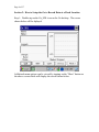
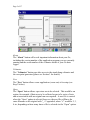
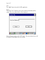
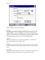
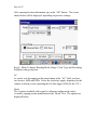
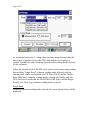
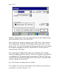
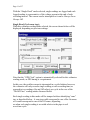
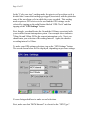
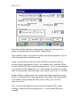
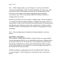
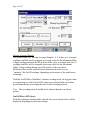
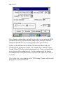
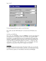
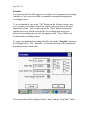
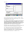
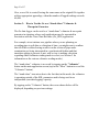
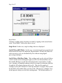
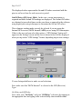
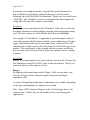
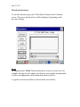
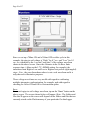
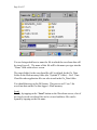
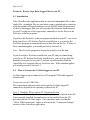
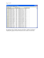
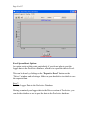
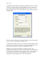
Page 1 of 37
Gx TIME CHART RECORDER APPLICATION
(Catalog # SFT133)
USER’S MANUAL
M. C. Miller Co., Inc.
11640 U.S. Highway 1, Sebastian, FL 32958
Page 2 of 37
CONTENTS
Page
Section 1: Introduction ……………………………………………….. 3
Section 2: How to Setup the Gx to Record Data at a Fixed Location … 4
Section 3: How to Use the Gx as a “Stand-Alone” Voltmeter and
Waveprint Generator ………………………………. 23
Section 4: How to Copy Data-logger Files to your PC
4.1
4.2
4.3
4.4
Introduction …………………………………………. 30
How to Connect the Gx to your PC …………………. 30
The Manual Approach ………………………………. 31
Using the Driver in the ProActive Application ……... 32
Page 3 of 37
Section 1: Introduction
In the “Gx Time Chart Recorder” application, voltages are logged as a
function of time at a fixed location and the voltage data are time-stamped.
The voltage data are time-stamped using either the data-logger’s internal
clock or the GPS clock. The clock option, or options, available for timestamping depends on the reading mode selected for the voltmeter.
For instance, either the internal clock or the GPS clock can be used to timestamp voltage data with the “Single Read” voltmeter reading mode selected,
only the internal clock can be used with the On/Off Pairs (D.S.P.) and the
On/Off Pairs (Min/Max) voltmeter reading modes selected and, finally, only
the GPS clock can be used with the On/Off Pairs (GPS Sync.) and the Single
Read (Cycle Zone Tag) voltmeter reading modes selected (please see
Section 2 for more details on the various voltmeter reading mode options).
Typically, time-stamped “structure-to-electrolyte” data collected over a
period of time are used to examine the impact of stray current on a structure.
Telluric current pick-up (and discharge) from a buried pipeline is an
example of stray current affecting a structure. Other examples include
current induced by DC railway and DC welding systems.
A particular consequence of such stray current is its affect on DC close
interval potential surveys (CIPS or CIS) conducted on buried pipelines, since
pipe-to-soil voltages can be significantly affected by stray current that’s
present in the soil during a survey.
Steps can be taken, however, to correct for such effects by setting up dataloggers at test stations that bracket a pipe section under survey in order to
collect time-stamped pipe-to-soil voltages as similarly time-stamped data are
being collected on a close interval potential survey. By doing so, CIPS data
can be compensated, in applications such as ProActive, for any spurious
effects due to stray current.
Consequently, one of the principal uses of the “Gx Time Chart Recorder”
application is to provide data that can be used to correct CIPS data, should
correction be required, i.e. should non-steady-state voltages be detected at
fixed locations in the vicinity of a pipe section under test.
Page 4 of 37
Section 2: How to Setup the Gx to Record Data at a Fixed Location
Step 1: Double-tap on the Gx_SDL icon on the Gx desktop. The screen
shown below will be diplayed.
Additional menu options can be viewed by tapping on the “More” button on
the above screen which will display the screen shown below.
Page 5 of 37
About
The “About” button will reveal important information about your Gx,
including the version number of the application program you are currently
running and the serial number of the voltmeter inside of your Gx datalogger.
Voltmeter
The “Voltmeter” button provides access to the stand-along voltmeter and
the waveprint generator (please see Section 3 for details).
New
The “New” button allows a new application (a new run) to be setup (see
Step 2 below).
Open
The “Open” button allows a previous run to be selected. This would be an
option, for example, if data were to be collected as part of a series of tests
and an association with an original run was required. A new file is created
when the “Open” option is selected, however, the new file will have the
same filename as the original with “_ #” appended, where “#” would be 2, 3,
4 etc, depending on how many times a file is selected via the “Open” option.
Page 6 of 37
Quit
The “Quit” button closes the Gx-SDL application.
Step 2:
Tap on the “New” button to create a file in which recorded data will be
stored. The screen shown below will be displayed.
Enter a filename and tap on the “OK” button. The screen shown below will
be displayed, depending on previous settings.
Page 7 of 37
Step 3: Establish test location information
Location:
By tapping on the menu button in the right-hand field, you can select either
“Station Number”, “Feet” or “Milepost” as the “units” for the location [or
“Station Number”, Meters” and “Kilometer post” if the “Use Metric” box is
checked. The numerical value (and its style) entered into the left-hand field
will depend on your selection of “units” in the right-hand field.
Pipeline:
If the test location involves a connection to a pipeline, you can enter the
name of the pipeline in the “Pipeline” field.
Device:
By tapping on the menu button in the “Device” field, you can select the type
of device at which you will be collecting data from the device type options
menu.
Description:
Text can be entered, if desired, in the “Desc” field in order to provide more
information on the test site location or on the nature of the test site.
Page 8 of 37
After entering location information, tap on the “OK” button. The screen
shown below will be displayed, depending on previous settings.
Step 4: Make Voltmeter Reading Mode, Range, Clock Type and Recording
Schedule setting selections
AC:
As can be seen by tapping on the menu button in the “AC” field, you have
two choices, 60Hz and 50Hz. Select the electricity supply frequency for the
country in which you are operating the Gx data-logger (60Hz for the U.S.).
Mode:
The 5 options available with regard to voltmeter reading mode can be
viewed by tapping on the menu button in the “Mode” box. The options are
displayed below.
Page 9 of 37
As mentioned in Section 1, voltage data are time-stamped using either the
data-logger’s internal clock or the GPS clock and the clock option, or
options, available for time-stamping depends on the reading mode selected
for the voltmeter.
Either the internal clock or the GPS clock can be used to time-stamp voltage
data with the “Single Read” voltmeter reading mode selected, only the
internal clock can be used with the On/Off Pairs (D.S.P.) and the On/Off
Pairs (Min/Max) voltmeter reading modes selected and, finally, only the
GPS clock can be used with the On/Off Pairs (GPS Sync.) and the Single
Read (Cycle Zone Tag) voltmeter reading modes selected.
Single Read:
With this voltmeter reading mode selected, the screen shown below will be
displayed.
Page 10 of 37
With the “Single Read” mode, the voltage data can be time-stamped using
either the Internal Clock or the GPS Clock.
If the “GPS Clock” option is selected via the “GPS Clock” radio button in
the “Timing Mode” field, the “GPS Settings” button on the above screen
will be active. The only GPS Settings related issue with regard to the Single
Read option is making sure that the “Internal MCM” receiver option is
selected for the “GPS Type”.
After selecting the “Single Read” mode, you would enter the recording
interval by tapping in the box labeled, “Interval” and typing in your desired
recording interval. By tapping on the menu button in “Interval” field, you
can select the units for the recording interval from a choice of milliseconds,
seconds, minutes, hours and days.
Note: The shortest recording interval is 100ms.
For example, if you wanted voltage data to be recorded every second, you
would select “seconds” and enter “1.0”.
Page 11 of 37
With the “Single Read” mode selected, single readings are logged and each
logged reading is representative of the voltage present at the end of each
recording interval. The current can be interrupted or it can be Always On or
Always Off.
Single Read (Cycle zone tags):
With this voltmeter reading mode selected, the screen shown below will be
displayed, depending on previous settings.
Note that the “GPS Clock” option is automatically selected for this voltmeter
reading mode, as GPS timing is a requirement.
In this case, the rectifier-current is interrupted in a cyclic fashion; however,
the voltmeter will only record a single reading at each recording time (as
opposed to two readings (On and Off values) per cycle in the case of the
“On/Off Pairs” reading modes discussed below
Each single reading in this mode will be stamped with an identifying “zone”
tag, as described below. A zone tag could correspond to one of the On zones
or it could correspond to one of the Off zones, depending
on when each single reading is recorded relative to the pipe-to-soil
waveform cycle.
Page 12 of 37
In the “Cycle zone tags” reading mode, the pipe-to-soil waveform cycle is
divided into 8 zones and readings get tagged (associated) with the particular
zone of the waveform cycle in which they were recorded. This reading
mode requires a GPS receiver to be used and the GPS settings can be
selected by tapping on the radial button labeled “GPS Clock” and then
tapping on the “GPS Settings” button.
First, though, you should enter the On and the Off times associated with
your rectifier-current-interruption system. Our example above indicates
700ms On and 300ms Off for the current interruption cycle. Next, you
should enter your selection of Recording Interval. Again, the shortest
recording interval is 100ms.
To make your GPS settings selections, tap on the “GPS Settings” button.
The screen shown below will be displayed, depending on previous settings.
You are being asked here to make several selections.
First, make sure that “MCM Internal” is selected as the “GPS Type”.
Page 13 of 37
On Delay and Off Delay:
Next, enter your “On Delay” and your “Off Delay” selections by tapping on
the appropriate box and typing in the selected delay time in milliseconds.
These delay time values are used to establish the “zones” of the cyclic pipeto-soil waveform.
For instance, you might determine prior to beginning the SDL application
that there is significant spiking in the pipe-to-soil waveform following Onto-Off and Off-to-On transitions (please see Section 3). In this case, you
could select “Off Delay” and “On Delay” times to correspond to the times
required for steady state (On and Off) voltages to be attained. By doing so,
you would be identifying the “zones” on the cyclic waveform that contain
the spiking. Consequently, since in the “Cycle zone tag” reading mode,
voltage data are tagged with the zone of the cycle in which the data was
recorded, you would be in a position, for example, to reject data that is
recorded in the zones where you know that spiking is occurring.
Downbeat
By tapping on the menu button in the “Downbeat” field, you can select the
downbeat schedule associated with the particular current interrupters being
used. The three options are: Each Minute, Each Hour and Midnight.
For example, if “Each Minute” is applicable to your interrupters, and you
select this option for the Downbeat schedule, you are indicating to the datalogger software that at the top of each minute, there will be an On to Off
transition (the rectifier current will switch from On to Off at the top of each
minute). This would mean, in this example, that the software would only
have to count back to the top of the last (previous) minute to have a timing
reference.
Cycle Start
Finally, if your interruption cycle starts with the current in the ON state (the
first transition is from ON to OFF), check off the box labeled, “Start Cycle”
(un-check this box if the opposite is true).
On/Off Pairs (DSP mode):
With this voltmeter reading mode selected, the screen shown below will be
displayed, depending on previous settings.
Page 14 of 37
Note that with this voltmeter reading mode selected, the Internal Clock
option is automatically selected for the Timing Mode.
This voltmeter mode is an option if rectifier-current interruption is to be ineffect during the data collection period.
Again, you should enter the On and the Off times associated with your
rectifier-current-interruption system. Our example above indicates 700ms
On and 300ms Off for the current interruption cycle. Next, you should enter
your selection of Recording Interval. For this mode, the shortest recording
interval is the period of the waveform cycle, which, in our case, is 1 second.
In this voltmeter reading mode, the software uses digital signal processing
(D.S.P.) to determine the voltage during the ON portion of the interruption
cycle and the voltage during the OFF portion of the cycle, for each
successive cycle.
Note: A measurable difference between the ON and the OFF voltage
readings is required for this reading mode, i.e. a measurable IR drop is
required.
Page 15 of 37
Note: In this reading mode, you do not have to concern yourself with
selecting recording times for the On and Off readings, for each cycle, with
respect to the On-to-Off transitions and the Off-to-On transitions of the
waveform, as the software determines appropriate locations on the
waveform for you. This is in contrast to the On/Off Pairs (GPS Sync.)
reading mode (see below).
With the On/Off Pairs (D.S.P) voltmeter reading mode, current interruption
is required and both On and Off readings are logged. The logged values are
representative of the On and Off values associated with the waveform period
immediately proceeding the end of each recording interval. Representative
On and Off values are determined by the software using digital processing
techniques.
Note: The recording interval should not be shorter than the waveform
period.
On/Off Pairs (Min/Max):
This voltmeter reading mode should be selected if you were using rectifier
current-interruption and there was considerable interference indicated on the
waveform. In such a case, in the absence of well-defined steps (IR drops),
the software determines an average value for the maxima and an average
value for the minima occurring in the waveform as being representative of
the On and the Off value per cycle.
With this voltmeter reading mode selected, an addition field (“Moving
Average Samples”) will be displayed, as indicated on the screen shown
below.
Page 16 of 37
Moving Average Samples
The default value for “Moving Average Samples” is 4. In this case, 4 sample
readings would be used to compute an average value for the Minimum (Min)
voltage reading during each OFF portion of the cyclic waveform and, also, 4
readings would be used to compute an average value for the Maximum
(Max) voltage reading during each ON portion of the waveform.
Different values can be entered for this parameter in order to try to
“optimize” the On/Off readings, depending on the nature of the interference
occurring.
With the On/Off Pairs (Min/Max) voltmeter reading mode, the logged values
are representative of the On and Off values associated with the waveform
period immediately proceeding the end of each recording interval.
Note: The recording interval should not be shorter than the waveform
period.
On/Off Pairs (GPS Sync):
With this voltmeter reading mode selected, the screen shown below will be
displayed, depending on previous settings.
Page 17 of 37
This voltmeter reading mode can only be selected if you are using the MCM
Internal GPS receiver (Internal MCM) AND current-interrupter switches
equipped with GPS receivers are being employed on your rectifiers.
Again, you should enter the On and the Off times associated with your
rectifier-current-interruption system. Our example above indicates 700ms
On and 300ms Off for the current interruption cycle. Next, you should enter
your selection of Recording Interval. For this reading mode, the shortest
recording interval is the period of the waveform cycle, which, in our case, is
1 second.
Also, in this case, you would tap on the “GPS Settings” button, which would
bring up the screen shown below.
Page 18 of 37
You are being asked here to make several selections.
First, make sure that “MCM Internal” is selected as the GPS (Receiver)
Type.
On Delay and Off Delay:
Next, enter your “On Delay” and your “Off Delay” selections by tapping on
the appropriate box and typing in the selected delay time in milliseconds.
For instance, you might determine prior to beginning the SDL application
that there is significant spiking in the pipe-to-soil waveform following Onto-Off and Off-to-On transitions (please see Section 3). In this case, you
could select “Off Delay” and “On Delay” times to correspond to the times
required for steady state (On and Off) voltages to be attained.
Downbeat
By tapping on the menu button in the “Downbeat” field, you can select the
downbeat schedule associated with the particular current interrupters being
used. The three options are: Each Minute, Each Hour and Midnight.
Page 19 of 37
For example, if “Each Minute” is applicable to your interrupters, and you
select this option for the Downbeat schedule, you are indicating to the datalogger software that at the top of each minute, there will be an On to Off
transition (the rectifier current will switch from On to Off at the top of each
minute). This would mean, in this example, that the software would only
have to count back to the top of the last (previous) minute to have a timing
reference.
Cycle Start
Finally, if your interruption cycle starts with the current in the ON state (the
first transition is from ON to OFF), check off the box labeled, “Start Cycle”
(un-check this box if the opposite is true).
With the On/Off Pairs (GPS Sync) voltmeter reading mode, current
interruption is required and both On and Off readings are logged. The logged
values are representative of the On and Off values associated with the
waveform period immediately proceeding the end of each recording interval.
However, in this case, the On and Off values are obtained at prescribed
times on the waveform (based on your On Delay and Off Delay values), as
opposed to the software using digital processing techniques to determine the
On and Off values.
Note: The recording interval should not be shorter than the waveform
period.
Range:
By tapping on the menu button in the “Range” field, you can make your
selection of range for the voltmeter together with associated input
impedance value.
A variety of Range/Input Impedance combinations are available, depending
on the type and magnitude of voltage to be recorded.
Note: Since all DC channels (Ranges) on the Gx data-logger have a fast
response time (<80ms), they are all suitable for fast cycle interruption
applications.
Page 20 of 37
Schedule:
You can setup the Gx data-logger to record data on a programmed recording
schedule, or, you can record data by manually starting and stopping the
recording process.
To record manually, tap on the “OK” button on the Settings screen (once
you’ve made your settings selections), which will return you to the main
application screen. You can then tap on the “Start” button on the main
application screen, which will start the Gx recording data using your
prescribed recording interval, and, by tapping on the “Stop’ button, you
would end the recording session.
To setup a programmed recording schedule, tap on the “Schedule” button on
the Settings screen. The “Schedule” screen shown below will be displayed,
depending on the current date.
The current date will be displayed in the “Start” and the “Stop Date” fields.
Page 21 of 37
Should a recording schedule be required on the current date, the time at
which the recording is to start and the time at which the recording is to stop
should be entered in the fields labeled, “Daily Start Time” and “Daily Stop”,
respectively.
You can highlight a field (hour, minute, second or AM/PM) and then either
tap on the up/down arrows to change the value or you can use the keyboard
to change the values.
As can be seen from the above screen, you can also program the “start
date” (the day the recordings will begin) and the “stop date” (the day the
recordings will end).
You can highlight a field (day, month or year) and then either tap on the
up/down arrows to change the value or you can use the keyboard to change
the values.
You can also select to skip recording data on certain days of the week, in a
multi-day recording process, by checking off the appropriate check boxes
associated with the day, or days, you’d like to skip in the “Skip Days” field.
To save your programmed recording schedule, tap on the “OK” button on
the “Schedule” screen which will return you to the “Settings” screen. By
tapping on the “OK” button on the “Settings” screen, the main application
screen (Gx_SDL screen) will be displayed as indicated below, depending on
the settings selected.
Page 22 of 37
The setup settings made for the above example were as follows: “Single
Read” mode for the voltmeter with a voltmeter “Range” of 5.7V. Also, the
recording interval was set at 1 second
Note: When a recording schedule is programmed, the “Start” button on
the main application screen needs to be tapped in order to “activate”
the program. “Start time wait” should be indicated in the “Status” field
(under the graph) which means that the software is waiting for your
programmed “Start” time to begin the data-logging process.
Each logged voltage value is displayed (in succession) in the “Logged” field
on the above screen, in addition to being displayed on the graph.
Note: Within a given run, new files are created each time the logging
process is stop and re-started, whether it’s done manually or via a
programmed recording schedule. Each of the files will have the same
filename as the original filename with “_ #” appended to the filename for
each successive file created, where “#” would be 2, 3, 4 etc.
Page 23 of 37
Also, a new file is created, having the same name as the original file together
with an appropriate appendage, when the number of logged readings exceeds
64,000.
Section 3:
How to Use the Gx as a “Stand-Alone” Voltmeter &
Waveprint Generator
The Gx data-logger can be used as a “stand-alone” voltmeter & waveprint
generator in situations where such applications may be warranted in
association with the Time Chart Recorder (Gx_SDL) application.
For example, at test stations on a pipeline where you are planning on
recording pipe-to-soil data as a function of time, you might want to confirm
that all of the rectifiers having an affect on the section of pipe under
examination are being interrupted in a synchronized fashion and that
transition spiking is present, or not, with a view to making a decision
regarding which voltmeter reading mode to select (see Section 2 for
information on the various voltmeter reading modes).
The “stand-alone” voltmeter is accessed by tapping on the “Voltmeter”
button on the main application screen (tap on the “More” button to reveal the
“Voltmeter” button).
The “stand-alone” term arises due to the fact that, in this mode, the voltmeter
is operating outside of the SDL parameters and is being used in an
independent (non-data-logging) capacity.
By tapping on the “Voltmeter” button, the screen shown below will be
displayed, depending on previous settings.
Page 24 of 37
Read Mode:
Voltmeter reading mode selections are made by tapping on the menu button
in the “Read Mode” field on the above screen.
Single Read: In this case, single reading values are displayed.
On/Off Pairs (DSP Mode): In this case, current interruption is required and
both On and Off values are displayed. Representative On and Off values for
each successive cycle are determined by the software using digital
processing techniques.
On/Off Pairs (Min/Max) Mode: This reading mode can be selected if there
is noise on the current interruption (pipe-to-soil) waveform and there are no
discernable IR drops (see the Waveform Generator section below). In this
case, a number of sampled readings would be averaged to determine both the
On and the Off voltages (during each cycle). The specific number of
readings used by the voltmeter to come up with these averaged values would
be dictated by the number that you enter in the “Moving Ave. Samples” box,
which appears when you select this reading mode. The default number is 4.
Page 25 of 37
The displayed values represent the On and Off values associated with the
pipe-to-soil waveform for each successive period.
On/Off Pairs (GPS Sync) Mode: In this case, current interruption is
required and both On and Off readings are displayed. The On and Off values
are obtained at prescribed times on the waveform, as opposed to the software
using digital processing techniques to determine the On and Off values.
This voltmeter reading mode can only be selected if you are using the
Internal GPS receiver (MCM Internal) AND you are using GPS interrupters.
If this is the case and you select this option, a “GPS Settings” button will
appear on the Settings screen and the screen shown below will be displayed
when you tap on the “GPS Settings” button, depending on previous settings.
You are being asked here to make several selections.
First, make sure that “MCM Internal” is selected as the GPS (Receiver)
Type.
On Delay and Off Delay:
Next, enter your “On Delay” and your “Off Delay” selections by tapping on
the appropriate box and typing in the selected delay time in milliseconds.
Page 26 of 37
For instance, you might determine, using the Waveprint Generator (see
below) that there is significant spiking in the pipe-to-soil waveform
following On-to-Off and Off-to-On transitions. In this case, you could select
“Off Delay” and “On Delay” times to correspond to the times required for
steady state (On and Off) voltages to be attained.
Downbeat
By tapping on the menu button in the “Downbeat” field, you can select the
downbeat schedule associated with the particular current interrupters being
used. The three options are: Each Minute, Each Hour and Midnight.
For example, if “Each Minute” is applicable to your interrupters, and you
select this option for the Downbeat schedule, you are indicating to the datalogger software that at the top of each minute, there will be an On to Off
transition (the rectifier current will switch from On to Off at the top of each
minute). This would mean, in this example, that the software would only
have to count back to the top of the last (previous) minute to have a timing
reference.
Cycle Start
Finally, if your interruption cycle starts with the current in the ON state (the
first transition is from ON to OFF), check off the box labeled, “Start Cycle”
(un-check this box if the opposite is true).
Range:
By tapping on the menu button in the “Range” field, you can make your
selection of range for the voltmeter together with associated input
impedance value.
A variety of Range/Input Impedance combinations are available, depending
on the type and magnitude of voltage to be recorded.
Note: Since all DC channels (Ranges) on the Gx data-logger have a fast
response time (<80ms), they are all suitable for fast cycle interruption
applications.
Page 27 of 37
Waveform Generator
To use this function, tap on the “WaveForm” button on the Voltmeter
screen. The screen shown below will be displayed, depending on the
previous settings.
Read:
By tapping on the “Read” button on the above screen, you can view, for
example, the pipe-to-soil voltage waveform at a test station, assuming that
you have the appropriate cable connections made to the Gx.
A typical waveform would be as shown in the screen below.
Page 28 of 37
Since we set up a 700ms ON and a 300ms OFF rectifier cycle in this
example, the pipe-to-soil voltage is “High” for 0.7 sec. and “Low” for 0.3
sec., as evidenced by the 1 second “snap shot” of the voltage waveform
shown in the above screen. Since the voltmeter in the Gx has a finite
response time (~80ms on the 5.7V, 400MΩ setting, for example), the
transitions from High to Low and Low to High are not perfect (right-angled)
steps. Note: the waveform shown above is not a real waveform and it is
only shown for illustrative purposes.
These voltage waveforms are very useful with regard to confirming
multiple-interrupter synchronization, for example, and with regard to
checking for On-to-Off and Off-to-On transition spikes.
Save:
To record a pipe-to-soil voltage waveform, tap on the “Save” button on the
above screen. The screen shown below will appear (Note: The folders and
files that’ll appear on the screen will depend on the folders and files that are
currently stored on the Flash memory of your particular Gx data-logger.
Page 29 of 37
You are being asked here to name the file in which the waveform data will
be stored (saved). The name of this file will be the name you type into the
“Name” field on the above screen.
The target folder for the waveform file will, by default, be the Gx_Data
folder on the Flash memory folder (the “SystemCF” folder). Note: Time
Chart Recorder application files are also stored in the Gx_Data folder.
You should then tap on the OK button. This process will “save” the
waveform data on the Gx data-logger’s Flash memory.
Load:
Finally, by tapping on the “Load” button on the Waveform screen, a list of
previously saved waveform files can be viewed and these files can be
opened by tapping on the file name.
Page 30 of 37
Section 4: How to Copy Data-Logger Files to your PC
4.1 Introduction
Time Chart Recorder application data are stored in independent files (either
single files, or multiple files per run (when a run is stopped and re-started or
when the number of logged readings exceeds 64,000) on the Flash memory
of the Gx data-logger, and, you can copy data files from the Flash memory
to your PC using one of two approaches; manually or via the Driver in the
ProActive software program.
If you have the ProActive software program installed on your PC, or you can
bring your Gx to a PC that has ProActive installed on it, you can use the
ProActive program to automatically access data files on the Gx. If either of
these situations applies, you would proceed to Section 4. 4.
Note: The ProActive program is required to actually view the data.
If you do not have ProActive installed on your PC and you cannot bring
your Gx to a PC that has ProActive installed on it, you can copy data files
manually from your Gx to your PC and you can subsequently send the
copied files to a recipient who is a ProActive user. If this situation applies,
you would proceed to Section 4. 3.
4.2
How to Connect the Gx Data-logger to your PC
Gx Data-loggers can be connected to a PC using the USB cable supplied
with the unit.
Connection via the USB Cable:
The requirements and procedures with regard to Gx Data-logger/PC
connectivity depend on the operating system of the PC.
Case 1: Windows XP (or earlier) PC Operating System
The Microsoft “ActiveSync” communication program is required on the PC.
If not currently installed, the application can be installed from the CD
provided with the Gx Data-logger. Once installed, make sure that the
“Allow USB Connections” option is selected in the “Connection Settings”
window of the ActiveSync application.
Page 31 of 37
Next, connect the USB cable from the Gx Data-logger to the PC and switch
ON the Gx (via the RED power button). The connection should be
automatic and you will be asked if you’d like to set up a partnership or not
between the Gx and the PC. Answer NO to this question, as the ability to
transfer file data is all that is required, as opposed to a synchronized
partnership. You can then exit the Activesync application.
If the connection is not established automatically, make sure that the
connection option on the Gx is “USB_Serial”, which it should be by default.
To do so, tap on the “Start” button on the Gx screen, tap, on “Settings”, tap
on “Control Panel” and double-tap on “PC Connection”. If “USB_Serial” is
not indicated, tap on the “Change Connection” button and select
“USB_Serial” from the drop down menu. Repeat the connection process.
Case 2: Windows Vista or Newer (such as Windows 7) PC Operating
System
The Gx Data-logger connects to these systems via the “Mobile Device
Center” which replaces the Activesync program on the PC side.
Make sure that the USB connection option is set up via the Mobile Device
Center. Connect the USB cable between the Gx Data-logger and the PC and
switch ON the Gx. The connection should be established automatically.
If the connection is not established automatically, make sure that the
connection option on the Gx is “USB_Serial”, which it should be by default.
To do so, tap on the “Start” button on the Gx screen, tap, on “Settings”, tap
on “Control Panel” and double-tap on “PC Connection”. If “USB_Serial” is
not indicated, tap on the “Change Connection” button and select
“USB_Serial” from the drop down menu. Repeat the connection process.
4. 3
The Manual Approach
Once you have established a connection between the Gx Data-logger and
your PC (see Section 4.2 above), proceed as follows:
*
•
•
•
•
Double-click on “My Computer” on your PC
Double-click on “Mobile Device”
Double-click on “SystemCF”
Double-click on “Gx_Data”
Right-click on the data file you wish to copy & select “Copy”
Page 32 of 37
• “Paste” the file into a local folder on your hard-drive
• Create a compressed (zipped) version of the file
You would now be in a position to send the compressed file via email, for
example, to a recipient who has access to the ProActive software program.
Note: Do not rename the data file prior to sending the file to the ProActive
user.
4. 4 Using the Driver in the ProActive Software Program
Step 1:
Create a folder on your PC’s hard-drive (perhaps in your “My Documents”
folder) that will be used to “permanently” save files copied from your datalogger. You might choose to name this folder something like, “Logger
Files”.
Step 2: Establish a connection between the Gx and your PC as outlined in
Section 4.2 above.
Step 3:
Double-click on the “ProActive” icon on your PC’s desktop screen.
This will open up ProActive’s main menu window. A window labeled
“Entire Database” will also be seen here. The suggested organization of
your database is discussed in the ProActive Training Manual.
Step 4:
Select “Data-Logger” and then “Time Charts” via the “Tools” menu in
ProActive.
This will open a window labeled “Data Logger: Get Time Chart Data”.
By clicking on the menu button in the “Data Logger” field, you can select
the data-logger (GX) from which you are copying the data file. The various
data-loggers currently supported by ProActive are offered as choices in the
menu list.
Finally, click on the “Go” button which will open the Gx Driver Window.
Page 33 of 37
Note: It may take a few seconds for the “Driver” Window to appear.
Step 5:
Identify the Data File to be Copied.
First, make sure that the “Logger Data” option is selected in the “Data Type”
field.
The “Get Data-logger Data from Gx” field on the “Gx Driver” window will
list all logger data files currently stored on your Gx’s Flash memory card.
Highlight the data file you would like to be copied to your PC. Also, checkoff the box labeled “Copy to Local Folder” and identify the target folder’s
location on your hard-drive in the field underneath using the “browse”
button.
This is the folder that you set up previously (Step 1 above) in which to save
the logger data files copied from your Gx.
Finally, click on the “Go” button on the Gx Driver window.
Note: Within a given run, new files are created each time the logging
process is stop and re-started, whether it’s done manually or via a
programmed recording schedule. Each of the files will have the same
filename as the original filename with “_ #” appended to the filename for
each successive file created, where “#” would be 2, 3, 4 etc.
Also, a new file is created, having the same name as the original file together
with an appropriate appendage, when the number of logged readings exceeds
64,000.
Step 6:
Examine the Time Chart Data Prior to Posting the Data to the ProActive
Database.
You will have actually completed the process of copying a logger data file to
a local folder on your PC by this point, using the Driver in ProActive.
However, before exiting the Driver, it is recommended that you examine
your data prior to posting the data to the ProActive database.
Page 34 of 37
To examine the recorded data via the Driver, click on the Driver window
which will be sitting behind the “Time Chart Post” window (see Step 7
below for information on using the “Time Chart Post” window to post the
data to the ProActive database).
The “Driver” window will again be shown but, in this case, there will be a
selection of page tabs, labeled as follows:
“Logger Info”, “Readings” and “Graph”.
By clicking on the “Logger Info” page tab, you can view your setup
selections (see Section 2).
By clicking on the “Readings” tab, you can view your time-stamped logger
data.
As an example, the window shown below displays (date and) time-stamped
“pipe-to-soil” data recorded at a test station using the “On/Off Pairs (DSP)”
voltmeter reading mode (hence the two readings (On and Off values)
displayed). The data were collected for a period of approximately two
minutes, with the recording time interval being 1 second.
Page 35 of 37
By tapping on the “Graph” page tab on the Driver window, the data are
displayed in graphical form as illustrated in the window shown below.
Page 36 of 37
Excel Spreadsheet Option:
An option exists at this point, particularly if you do not plan to post the
logger data to the ProActive database, which is to export the data to Excel.
This can be done by clicking on the “Export to Excel” button on the
“Driver” window and selecting a folder on your hard-drive in which to save
the exported data.
Step 7:
Post the Logger Data to the ProActive Database.
Having examined your logger data in the Driver section of ProActive, you
can decide whether or not to post the data to the ProActive database.
Page 37 of 37
To post the data to the ProActive database, you would “retrieve” the “Time
Chart Post” window, that’ll be sitting behind the Gx Driver window, and
you would use this window to target a particular test site “device” in the
ProActive database tree. This would be the test site at which you recorded
the logger data
The above window allows you to associate the logger data with a particular
test site “device” in your ProActive database tree.
As indicated in the above window, you can either select the pipeline, station
number and site type for the posting or you can drag and drop the test site
device from your database tree into the “Matching Site” field.
With the test site properly identified, you would click on the “Save
Readings” button on the above window, which will post the time chart data
to the database in association with the targeted test site. You can then view
the time chart data in ProActive by opening the “Details Form” for the
targeted test site and clicking on the “Time Chart” page tab.