1
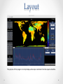
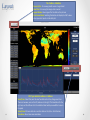
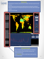
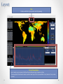
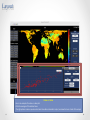
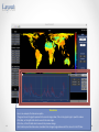
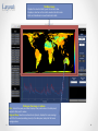
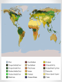
Aquarius Time Series Guide / User Manual Instructions This so'ware was developed using Matlab 2014a. In order to run this so'ware, you should at least have the 2014a version (no guarantee that is will work on later versions). To run the Aquarius Time Series Applica4on: -‐Double click on the Run.m file located in the Aquarius folder. This will trigger Matlab to open. -‐If there are not enough available licenses on the network, then Matlab will throw an error window. If this happens, simply try again later when there are less JPL employees using Matlab. -‐Once Matlab is open and the code is showing, there are two ways to complete the next step. Click the ‘Run’ buDon (located in the editor toolbar at the top) OR Type Run in the command window, and press Enter. -‐Matlab might ask you to change to the correct folder. If it does, click Change Folder/Accept -‐The program will then run. A loading window will inform you that the data is being loaded into the workspace. Once it is finished loading the data, the applicaHon will be displayed. Layout The purpose of this program is to help display and analyze radar data from the Aquarius Satellite. Layout The Toolbar – 5 bu;ons Zoom in/Out : For viewing smaller areas in larger detail Hand Tool: For moving the image while zoomed Legend Bu;on: View a legend for the data on the plot axis Data Cursor Mode: SelecHng this buDon will display the X & Y values when you select points on the data plot Plot Type Selec4on bu;ons -‐ 3 Bu;ons Value/Time : Select this panel to view Two data sets as they change over Hme. There are two axes, one on the leQ, and one on the right. The blue data is for the right axis, and the leQ axis is for the red data. Select what you would like to see in the panel Value/Value: Plot one data set vs. another data set. Ex (HH vs. Soil Moisture). Time Series: Run a Hme series simulaHon Layout Data Display Panel -‐Displays what pixel, or area of pixels, you have selected to view (2 different pixels will give two opposite corners of a selected area). -‐Displays the single value (or mean average value & standard deviaHon) of a selected pixel (or selected area). -‐Displays the corresponding date for the image displayed (changes with every new image, where each new image is a new week). -‐Change color limits of the image Image Type Selec4on Bu;ons -‐Here, you can select what type of data you would like to view. Choose from viewing raw radar data, correlaHon of two different radar types, or land classificaHon parameter images. -‐See the Data DescripHon slides for more details about each data type, and how the the data was developed. Layout Title Displays what data type you are currently viewing Plot and View Op4ons -‐Here is where you can view a plot of how the selected point/area changes over Hme. -‐The view opHons Check boxes is where you Select what type of Plot you would like to see. (value vs. Hme, or value vs. value) Layout Value vs. Value -‐Here is an example of a value vs. value plot. -‐Plots the averages of the selected area. -‐The right opHons is where you can select what two data combinaHon to plot, and view the linear trend of the output. Layout Time Series -‐Here is an example of a Hme series opHon. -‐The green line on the graph represents the current image index. Click on the graph to go to specific indexes. -‐Click Next, or the right slider bar to move to the next image. -‐Click Prev, or the leQ slider bar to move to the previous image. -‐Start and stop control a Hme series simulaHon that changes image indexes with the rate set in the FPS box. Layout The Main Image -‐Displays the selected data type at the current index. -‐Displays a color bar on the side to visualize the data scale. -‐Slider on the boDom to move from slide to slide. Clicking on the Image – 2 op4ons Click : Selects the pixel you clicked, displays that pixels value in the data panel, and plots that point’s values. Drag and Drop: Selects an enclosed area of pixels, displays the mean average and STD of the area (excluding ocean) in the data panel, and plots that areas average values. Data Information The data that gets loaded into the applicaHon is stored as a .mat file. The reason for this is to can keep all the data and variables in one locaHon. CompuHng them all at once saves Hme and leaves less work for the applicaHon. The Data is saved as AquariusWeeklyData.mat. It contains several series of 130 images -‐ (Sept, 2011 –> Feb, 2014, @weekly intervals). Each image has the dimensions 406x964. AquariusWeeklyData.mat contains the following: Radar Polarimetry -‐ HH -‐ VV -‐ HV -‐ RVI -‐ HH Wetness Parameter/Scale -‐ HV Wetness Parameter/Scale -‐ VV Wetness Parameter/Scale -‐ RVI Wetness Parameter/Scale CorrelaHon Images -‐ HH & HV CorrelaHon -‐ HH & VV CorrelaHon -‐ HV & VV CorrelaHon -‐ HH & HV Scale CorrelaHon -‐ HH & VV Scale CorrelaHon -‐ HV & VV Scale CorrelaHon -‐ RVI & HV Scale CorrelaHon -‐ RVI & VV Scale CorrelaHon -‐ RVI & VV Scale CorrelaHon Land ClassificaHon -‐ Sample Land ClassificaHon Image -‐ Soil Moisture data (SM) -‐ A & B values (From HH & SM, every 6 images) -‐ A & B values (From HV & SM, every 6 images) -‐ A & B values (From VV & SM, every 6 images) -‐ A & B Avg values (From HH & SM, EnHre series) -‐ A & B Avg values (From HV & SM, EnHre series) -‐ A & B Avg values (From VV & SM, EnHre series) Other -‐ ΔHH > ΔHV -‐ ΔHH > ΔVV -‐ ΔHV > ΔVV -‐ HH / VV -‐BadData (to keep track of bad data & ocean locaKons, not visible) Data Info Radar Polarimetry The Radar data (HH, HV, VV) is a 3D array with the dimensions 406x964x130, represenHng 130 pictures with the resoluHon 406x964. -‐ -‐ Scale is from -‐50 -‐> 10. Data is in db The Radar Vegeta4on Index data (RVI) is 406x964x130. (Normalized HV) -‐ Scale is from 0-‐1 -‐ -‐ Data is linear Each pixel’s value is obtained from the following equaHon: db-‐>linear before compuKng RVI (x, y ,t) = 8 * HV(x ,y, t) _ HH(x, y, t ) + VV(x, y, t ) + 2*HV(x, y, t ) The Wetness Parameter / Scale data (HH Scale, HV Scale, VV Scale, RVI Scale) are 3D arrays with the dimensions 406x964x130, represenHng 130 pictures with the resoluHon 406x964. -‐ -‐ -‐ Scale is from 0 -‐ 1 Data is Linear Each pixel’s value is obtained from the following equaHon: HHParameter(x, y ,t )= _HH(x ,y, t ) -‐ Min( HH(x, y, : ) ) (Max(HH(x, y, :) -‐ Min( HH(x, y, : ) ) : = iteraKon through enKre data Data Info Correlation Images The Correla4on Images are single images that display each pixel’s correlaHon between two types of data, over the whole Hme span (130 images, 2 years) -‐ -‐ Scale is from 0 -‐> 1 (406x964x1) Example (HH & VV CorrelaKon) For each pixel( x, y) CorrHHVV(x, y) = corr2( HH(x, y, : ), VV(X, Y, : ) ) corr2 is a built in Matlab funcKon from the image staKsKcs toolbox : = iteraKon through enKre data CorrelaHon Images -‐ HH & HV CorrelaHon -‐ HH & VV CorrelaHon -‐ HV & VV CorrelaHon -‐ HH & HV Scale CorrelaHon -‐ HH & VV Scale CorrelaHon -‐ HV & VV Scale CorrelaHon -‐ RVI & HV Scale CorrelaHon -‐ RVI & VV Scale CorrelaHon -‐ RVI & VV Scale CorrelaHon -‐ HH & SM CorrelaHon -‐ VV & SM CorrelaHon -‐ HV & SM CorrelaHon Data Info Land Classification Soil Moisture data ( SM ) -‐ Data originally in Lat/Long coordinates(180x360). -‐smap2ease funcKon to transform to 406X964 grid, hence the lower looking resoluKon -‐ Scale is from 0-‐1, -‐ Data obtained from hDp://nsidc.org/data/AQ3_WKSM Bindlish, R. and T. Jackson. 2013. Aquarius L3 Gridded 1-‐Degree Weekly Soil Moisture. Version 2. Boulder, Colorado USA: NASA DAAC at the NaHonal Snow and Ice Data Center. Land Classifica4on Sample Image -‐ Sample image of past land classificaHon. -‐smap2ease funcKon to transform to 406X964 grid -‐Last slide of this guide will show the scale and classificaKon types. A & B Land Values ( A(HH), B(HH), A(HV), B(HV), A(VV), B(VV), and series averages. ) -‐ A and B values represent constants that are common among each terrain type -‐ A and B images are 3D arrays with the dimensions 406x964x130, but each image is repeated 4 Hmes (32 different images) -‐ Each pixel’s value is obtained from the following equaHon: For every 6 images, (and enKre series for averages) temphh(1:4,1) = HH(x, y, 1:4); tempsm (1:4,1) = SM(x, y, 1:4); f = fit(temphh, tempsm, 'Poly1'); %Linear least square fit 6, pixels in Hme HHA(x, y, 1:4) = f.p1(1); %Slope HHB(x, y, 1:4) = f.p2(1); %Y-‐ Intercept : = iterate through the range Data Info Other Delta Data (ΔHH, ΔHV, ΔVV) -‐ An array of values (406x964x129) where each point is the difference in value between the current image, and the next Hme image -‐ Only visible in the plot Delta Images ( ΔHH>ΔHV, ΔHH>ΔVV, ΔHV>ΔVV ) -‐ Creates an image while looking at the difference between two Δ data types. -‐ 406x964x1 -‐ Each pixels value is obtained from the following equaHon: For each pixel For t=1:129 if ΔHH(x, y, t) > ΔHV(x, y, t) DHHDHV(x, y) += 1; else DHHDHV(x, y) -‐= 1; %Increment the current value %Decrement the current value HH / VV -‐ An array of images generated by dividing a pixels HH value by the corresponding VV value. -‐Division in linear scale is equal to subtracKon in logarithmic scale. -‐ 406x964x130 (linearly scaled example) For each pixel & image HHVV(x, y, t) = HH(x, y, t) / VV(x, y, t); Other Information Other functions: LoadData -‐‑ Reads raw data, and creates the datasets previously listed LoadNewFiles -‐‑ Loads the path and filenames of the raw data smapease2forward -‐‑ Convert between different grids smapease2inverse -‐‑ Convert between different grids maxCustom -‐‑ A custom max function that ignores when a value is bad data minCustom -‐‑ A custom max function that ignores when a value is bad data custlinfit -‐‑ A custom linear regression fit function for faster computation. -‐‑For more information, view the code file. Contact Any quesHons or issues, please contact Robert Schneider (8650) [email protected] 818-‐354-‐3678 321-‐225N [email protected] 818-‐319-‐5904(mobile)