1
Address:
Tel
Fax:
N-7034 Trondheim,
NORWAY.
+47 7359 5611
+47 7359 2660
COMMENTS ARE INVITED
Release Notes
USFOS Version 7-6
SINTEF Structural Engineering
FOR YOUR ATTENTION
MEMO CONCERNS
AS AGREED
FOR YOUR INFORMATION
MEMO
DISTRIBUTION
Members of USFOS user group
x
ONE COPY TO RECORDS OFFICE
FILE CODE
CLASSIFICATION
Open
ELECTRONIC FILE CODE
PROJECT NO.
DATE
22L050
1999-04-20
PERSON RESPONSIBLE/AUTHOR
Tore Holmås
NUMBER OF PAGES
18
Release notes
USFOS 7-6 1999
Contents:
1.
INTRODUCTION ..........................................................................................................................................2
2.
CONTENTS OF CD-ROM............................................................................................................................2
2.1.
2.2.
2.3.
2.4.
OVERVIEW ....................................................................................................................................................2
NEW VERSIONS OF THE PROGRAM CODES......................................................................................................3
MANUAL.......................................................................................................................................................4
EXAMPLES ....................................................................................................................................................4
3.
INPUT FILE FORMATS...............................................................................................................................5
4.
NEW FEATURES ..........................................................................................................................................6
4.1.
4.2.
4.3.
4.4.
4.5.
4.6.
5.
SHELL ELEMENT ...........................................................................................................................................6
SHELL FORMULATION FOR BEAMS.................................................................................................................8
EXTREME WAVE CALCULATION/AUTOMATIC MEMBER IMPERFECTIONS .......................................................9
PILE – SOIL / AUTOMATIC GENERATION OF PILES AND SOIL CAPACITY ........................................................12
DYNAMIC ANALYSIS RESULTS. TIME SERIES ..............................................................................................14
IMPACT ANALYSIS INCLUDING “DASH-POT” DAMPERS ................................................................................16
NEW/MODIFIED INPUT IDENTIFIERS.................................................................................................18
This memo contains project information and preliminary results as a basis for final report(s).
SINTEF accepts no responsibility of this memo and no part of it may be copied.
2
____________________________________________________________________________
1.
Introduction
The current version of USFOS (version 7-6, 99-04-20) is the final release of the 97-98 user group
development period.
The 7-6 version is the USFOS version, which will be used when the next millennium is entered.
As USFOS does not use date as input to the calculations (print of time for analysis initiation
only), the change from year 1999 to 2000 is assumed to cause no problems.
By artificially changing the date to the year 2000 one customer has tested the USFOS package on
their own computers with following conclusion: “We have successfully tested USFOS , XFOS
and POSTFOS thru 2-3 crucial date changes and has worked in all cases.”
The current release with date 1999-04-20 contains following:
CD-ROM
Updates of User’s Manual
Release Notes (this MEMO)
2.
2.1.
Contents of CD-ROM
Overview
The CD contains documentation, examples and new versions of the program codes, and the
organisation is described in Figure 2.1-1. Both UNIX and NT solutions are collected in the same
CD.
Figure 2.1-1 Contents of CD-ROM
______________________________________________________________________________________________________
Release Notes USFOS version 7-6
SINTEF 1999-04-20
3
____________________________________________________________________________
2.2.
New versions of the program codes
Under each file folder (f ex “USFOS_for_Windows_NT4.0”), two folders, (bin and etc) are
located. The “bin” folder contains the program code, while the “etc” folder contains set up
files.
Figure 2.2-1 Program Code located in “bin” folder
Figure 2.2-2 Files in “etc” folder. NT (to the left) and UNIX (to the right)
Installation on UNIX:
Create a root directory for USFOS, (the new “USFOS_HOME ” directory)
Copy the actual “bin” and “etc” directories to USFOS_HOME
Copy the “Examples_UNIX” and “Document” directories to USFOS_HOME.
Define the USFOS_HOME variable in the USFOS.cshrc/USFOS.kshrc files
Figure 2.2-3 Contents of "$USFOS_HOME" folder after installation
______________________________________________________________________________________________________
Release Notes USFOS version 7-6
SINTEF 1999-04-20
4
____________________________________________________________________________
Installation on Windows NT 4.0
Copy the new “.exe” files located in the “bin” folder to the existing “USFOS_HOME/bin”
folder
Copy the new “postfos.inca” file located in the “etc” folder to the existing
“USFOS_HOME/etc” folder
Copy the “Examples_PC” and “Document” folders to the existing USFOS_HOME.
NOTE ! : If USFOS has never been installed on NT before, please contact SINTEF.
For all systems:
Copy the file: “USFOS.key” (delivered on a separate diskette) to the actual
“USFOS_HOME/etc” directory.
2.3.
Manual
The User’s manual is updated, and (paper) copies of the actual pages are delivered. In addition,
the most important part of the manual, the “Input Description” is available for “on-line”
reading using f ex. Adobe Acrobat Reader or any other "PDF readers".
A free "PDF-reader" is available on www.adobe.com .
2.4.
Examples
Approx. 40 examples are given under the “Examples” directories. The contents of the UNIX and
PC examples are identical, (the only reason for having two folders is due to computer
compatibility, UNIX and PC represent the files differently).
The input files are located in separate folders, one example per folder, see Figure 2.4-1. In each
folder, following files are found:
Head.fem : USFOS control parameters
Stru.fem : Structure and load description in either SESAM or UFO file format. In some cases
both SESAM and UFO formats are given for the same example, and then the “strufile” has a postfix, u for UFO and s for SESAM. Any of the two variants
(stru_u.fem or stru_s.fem) should produce the same results. The USFOS control
parameters are unaffected by the file format used to describe the structure and
loads. (See also Chapter 3).
______________________________________________________________________________________________________
Release Notes USFOS version 7-6
SINTEF 1999-04-20
5
____________________________________________________________________________
Figure 2.4-1 Example folders available for UNIX and NT( PC)
3.
Input File Formats
In the current version of the User’s manual, one chapter describing the UFO file format is added.
The UFO file format is used to describe the same type of information, which normally is
described in SESAM file format, and has been used since 1994 by non-SESAM users. The type of
information is: Nodal ID’s, Coordinates and Boundary conditions, Element ID’s, connectivity
and properties etc. USFOS recognises the file format automatically, and the results are
unaffected by the structural/load file format used. However, mixing commands from the two
input formats are not possible.
Figure 2.4-1 Input files to USFOS
______________________________________________________________________________________________________
Release Notes USFOS version 7-6
SINTEF 1999-04-20
6
____________________________________________________________________________
In the USFOS User’s manuals, following sections are found:
6.3
6.4
6.5
USFOS Control Parameters
SESAM Structure and Load
UFO
Structure and Load
Following “style guide” is recommended see Figure 2.4-1:
Use the “USFOS control file” for the USFOS control parameters.
Use the “Structural file” for the structure and load input (described in either SESAM or UFO).
Sometimes it’s convenient to spread the structure/load input in two files (“Structure file”
and “Load file”).
4.
4.1.
New Features
Shell Element
From version 7-6, a non linear triangular shell element is available. The element is specified
through general SESAM input format, element type 25, or using the TRISHELL command (UFO
input). The thickness is specified similar to the existing membrane element. The non linear
material parameters are given in the "usual" MISOIEP record. Both concentrated load,
conservative distributed load and pressure load are available. In Table 4.1-1, the necessary
input records are given for both file formats.
Figure 4.1-1 Non linear shell element in USFOS. (Example tri_shell_joint)
______________________________________________________________________________________________________
Release Notes USFOS version 7-6
SINTEF 1999-04-20
7
____________________________________________________________________________
Item
SESAM file format
UFO file format
Element definition
Plate thickness
Material properties
Concentrated (nodal) Load
Pressure load (non-conservative)
Distributed (conservative) load
GELMNT1/GELREF1
TRISHELL
GELTH
PLTHICK
MISOIEP
MISOIEP
BNLOAD
NODELOAD
BEUSLO
PRESSURE
SHELLOAD
Table 4.1-1 Input records for triangular shell element
For more detailed description, see User's manual Ch. 6. See also following example folders:
tri_shell_1
tri_shell_2
tri_shell_joint
tri_shell_load
Result presentation:
The results for the shell element is presented in XFOS and available element results are plastic
strain and plastic utilisation. These result types are new, and are accessed through the new
"button":
GENERAL
ELEMENT
In Figure 4.1-2, the dialogue box used for shell element selection is shown.
Figure 4.1-2 Selecting Shell Element Result
______________________________________________________________________________________________________
Release Notes USFOS version 7-6
SINTEF 1999-04-20
8
____________________________________________________________________________
By default, no element mesh is shown on the model image, but using the Verify/Show Mesh
option as shown in Figure 4.1-3, the user may switch on the mesh. The same button is used to
switch off the mesh visualization.
Figure 4.1-3 Switching ON/OFF mesh visualization
4.2.
Shell formulation for beams
In addition to having the triangular, shell element available directly "one by one" as an ordinary
element, the shell element is possible to access through the shell sub structure option. An
ordinary beam element (pipe, box etc) is then represented by shell elements (in stead of the
normal beam formulation, see Figure 4.2-1). As the physical member is represented by shell
elements, effects like local buckling, torsion buckling, etc is predicted with high accuracy. The
necessary commands (subshell and meshpipe) used to define one "shell-beam" element are
described in figure Table 4.2-1overleaf.
Figure 4.2-1 Shell formulation on selected beam element
Several simple examples are given on the CD-ROM:
ssh_cantilever
ssh_col_I
ssh_col_pipe
ssh_jac
______________________________________________________________________________________________________
Release Notes USFOS version 7-6
SINTEF 1999-04-20
9
____________________________________________________________________________
'
'
SUBSHELL
'
'
MESHPIPE
- Use Shell_Beam for elem 12
Elem_Id
12
- Define mesh density
n_Length
6
n_Circ
12
Elem_Id
12
Table 4.2-1 Input commands defining shell formulation on beam elements
4.3.
Extreme Wave calculation/Automatic member imperfections
Modules for calculation of hydrodynamic forces are included in USFOS. This means that using
separate wave load pre processor is not needed. Using the USFOS hydrodynamic in connection
with static "push over" analysis will typically contain following:
Specify the actual wave (type, height, period, direction…)
Specify the corresponding current (if any)
Switch on buoyancy (optional)
Specify criterion to be used for selecting worst wave position (max base shear or max
overturning moment)
Direction of wave
Direction of Wave
Figure 4.3-1 Automatic member imperfection according to wave force direction
will then step through the actual wave and identify the worst wave position (the position
causing the highest base shear or overturning moment). The hydrodynamic forces from this
wave phase (position) are saved (in memory) to be used in the pushover analysis. The
calculated buoyancy forces are possible to separate from the other hydrodynamic forces, and
the user may specify how to use the buoyancy forces, (add to an existing deadweight loadcase
etc.).
USFOS
______________________________________________________________________________________________________
Release Notes USFOS version 7-6
SINTEF 1999-04-20
10
____________________________________________________________________________
Applying member imperfections, one by one, is a time consuming task, but by using the new
option CINIDEF, the correct member imperfection is applied automatically for all beam
elements. The most common buckling curves are available defining the size of the
imperfection, (see User's manual Ch. 6). The direction of the imperfections follow the direction
of the loads for a specified load case.
In Figure 4.3-1, the jacket to the right is exposed to waves with direction 45°, while the jacket
to the left is exposed to a wave with opposite direction (225°). It is seen that the direction of the
imperfections are opposite in the two cases (size is scaled).
All necessary input is shown in Table 4.3-1, and it should be noted that these few commands
replace 1000's of input lines and use of separate wave load pre-processor / load files.
Comments to the input given in Table 4.1-1 (see also example folder wave_maxwav):
Load case 1 is used for "dead weight" and calculated buoyancy
Load case 2 is used for the extreme wave
Load case 1 is not scaled beyond factor 1.0 (that’s why the calculated buoyancy forces is
separated from the other hydro. forces and added to this load case). Load case 2 forces are
scaled to platform collapse.
The direction of the member imperfections (CINIDEF par. no 2 and 3) follows the direction
of the member forces defined by load case 2 (which is the calculated wave forces).
The size of the imperfection (CINIDEF par. no 1) is calculated according to "Chen column
curve".
A Stoke 5'th wave with height 25m, period 16s, 45° direction is applied. The sea surface is
located for global Z-coordinate=0.0. Water depth is 100m.
A current profile with peak value 2 m/s is defined with same direction as the wave. From
depth 20m (Z=-20m relative to the sea surface), the current is reduces linearly.
The actual wave is 'stepped through' the structure with time increment 1 s. The wave
position giving the highest base shear in the interval Time = 0 -20s is used in the "push
over" analysis.
NOTE
As all hydrodynamic calculations are using SI units, the forces are calculated in
N (Newton). If f ex. MN is used as force unit, the wave forces must be scaled
before they are used in the "pushover" analysis. The command WAVMXSCL
<factor> is used, (see also User's manual, Ch 6). In the current example, the
wave forces are scaled with a factor 1.3 (just for demo purpose).
For both the buoyancy forces and the wave forces, it is possible to print the calculated
forces to separate files, but in the example, printing is switched off (nowrite).
______________________________________________________________________________________________________
Release Notes USFOS version 7-6
SINTEF 1999-04-20
11
____________________________________________________________________________
' ---------------------------------------------------------------------'
Lcomb 1 is gravity loads and static deck loads+calculated buoyancy,
'
Lcomb 2 is Stoke Wave 45 deg diretion
' ---------------------------------------------------------------------'
nloads
npostp
mxpstp
mxpdis
CUSFOS
10
15
1.00
0.05
'
lcomb
lfact
mxld
nstep
minstp
1
1.0
1.0
10
0.05
! Dead + Buoyancy
2
0.5
3.0
50
0.001
! Wave
2
0.1
6.0
100
0.001
! Wave
'
' ---------------------------------------------------------------------'
Apply automatic out of straightness.
'
Use loads from Waves (lcase 2)
' ---------------------------------------------------------------------'
Size
Pat
LoadCase
cInidef
70
1
2
'
' ---------------------------------------------------------------------'
Separate Bouyancy from wave forces.
'
Add Buoyancy to load case 1
' ---------------------------------------------------------------------'
'
lCase
Option
BUOYANCY
1
noWrite
'
'
- Define Wave:
'
'
Ildcs <type>
H
Period
Direction Phase Surf_Lev Depth
WAVEDATA
2
Stoke 25.0
16.0
45
0.0
0.0
100
'
'
Ildcs Speed Direction Surf_Lev Depth
[Profile]
CURRENT
2
2
45
0.0
100
0.0 1.0
-20.0 1.0
-100.0 0.0
-110.0 0.0
'
' ---------------------------------------------------------------------'
Identify Worst Phase (Max Base Shear) and do not create a loadfile
' ---------------------------------------------------------------------'
Criterion
dT
EndT
Write
MaxWave
Baseshear 1.0
20.0 noWrite
'
' ---------------------------------------------------------------------'
Scale the Wave load. This option is required when Force Unit is not N.
'
(generated wave loads are always using Newton).
'
In this demo case, scale by 1.3 :
' ---------------------------------------------------------------------WavMxScl
1.3
Table 4.3-1 Input for automatic wave calculations and automatic member imperfections
______________________________________________________________________________________________________
Release Notes USFOS version 7-6
SINTEF 1999-04-20
12
____________________________________________________________________________
4.4.
Pile – Soil / Automatic generation of piles and soil capacity
The automatic generation of piles and corresponding soil capacities is a powerful option, which
requires a few input lines only. The user's structure ends at "mud line", and all elements below
mud line are generated automatically by USFOS, see Figure 4.4-1. In Table 4.4-1 overleaf, the
necessary commands used to produce the foundation model shown in the figure are given.
See also the example in folder PSI_2.
User’s Strucutrual Model
Generated by USFOS
Figure 4.4-1 Automatic generation of piles and soil capacity
Comments to the input in Table 4.4-1:
The foundation consists of 4 pile clusters, each with 7 piles, and 4 single piles.
This foundation is defined as 8 PILE elements, which refer to one of the two PILEGEO
records.
PILEGEO number 1 consists of 7 pipes with diameter 1.22m. The individual positions are
specified through local Y- and Z-co ordinates referring to the PILE local axis.
The PILE local x-axis goes (downwards) from the pile head towards the pile tip.
PILEGEO number 2 is a single pile, here defined as a group with only one pipe in the centre
of the pile element axis. (The single pile option could also been used, see UM Ch 6).
______________________________________________________________________________________________________
Release Notes USFOS version 7-6
SINTEF 1999-04-20
13
____________________________________________________________________________
For all the 8 piles, the same soil exists (refer all to the same SOILCHAR record)
The SOILCHAR is specified with 3 clay layers and 3 sand layers. However, in order to obtain
a reasonable element density in the rather thick sand layer no. 2 (-24.1 to -48.8m), the same
soil property (no. 501) is referred to three times. (The soil spring is inserted in the middle of
the layers defined under SOILCHAR.
The soil strength is calculated according to API 1993 by specifying the geotechnical data in
the command API_SOIL.
'
Elem ID
1
2
3
4
5
6
7
8
PILE
PILE
PILE
PILE
PILE
PILE
PILE
PILE
'
''
PILEGEO
'
PILEGEO
'
SOILCHAR
'
'
API_SOIL
API_SOIL
API_SOIL
API_SOIL
'
np2
1001
1002
1003
1004
1005
1006
1007
1008
Soil ID
10
10
10
10
10
10
10
10
Pile_mat
99
99
99
99
99
99
99
99
ID
1
Type
2
Do
1.22
T
0.05
Npile
7
ID
2
Type
2
Do
1.22
T
0.05
Npile
1
ID
10
ID
101
201
301
401
np1
1
2
3
4
5
6
7
8
Type Z_Mud D_ref Ffac
API -93.725 1.0 1.0
Type
SoftClay
StifClay
StifClay
StifClay
ID typ
API_SOIL 501 Sand
API_SOIL 601 Sand
load
Static
Static
Static
Static
load
Static
Static
Gam
9500
9500
9500
9500
Gam
8000
8000
Lfac
1.0
Plug Su
1
50E3
1 120E3
1 150E3
1 190E3
Plug Phi
0
33
0
37
Pile_geo lcoor
1
0
2
0
2
0
1
0
1
0
2
0
2
0
1
0
Y_loc
0.0
2.1
3.0
0.6
-1.65
-2.5
-1.5
Y_loc
0.0
Z1
-1.0
-5.2
-12.5
-18.3
-24.1
-28.3
-42.7
-48.8
Z2
-5.2
-12.5
-18.3
-24.1
-28.3
-42.7
-48.8
-67.0
eps50
0.013
0.012
0.010
0.019
Delta
22
26
APIJ
0.25
0.25
0.25
0.25
rNq
22
23
Imper
Z_loc
0.0
2.1
-1.4
-2.5
-1.65
0.6
2.7
Z_loc
0.0
API_Soil
101
201
301
401
501
501
501
601
Tresf
0.74
0.72
0.73
0.75
ID
! Clay
! Clay
! Clay
! Sand
! Sand
! Sand
! Sand
! Sand
QPLim
0.2E6
1.2E6
1.0E6
1.9E6
iDyn
0
0
0
0
QPlim
1.4E7
1.1E7
iDyn
0
0
Table 4.4-1 Input for automatic calculation of piles and soil capacities
______________________________________________________________________________________________________
Release Notes USFOS version 7-6
SINTEF 1999-04-20
14
____________________________________________________________________________
4.5.
Dynamic Analysis results. Time Series
A dynamic analysis may involve a large number of analysis steps (1000 - 100 000), and saving
of analysis results is then a challenge. It is then necessary to select a few results, which could
be saved every analysis step, while the rest of the results could be saved more seldom. In this
way, the user obtain following:
High density on the time series of the selected (most important) results
Acceptable density on the results presented in XFOS for inspection of the global behaviour
of the structure (f ex generation of animation etc).
The few, selected result quantities are stored in a separate file with extension .dyn in addition to
the usual .raf file. The dynamic results are accessed from XFOS through the
result/dynamic_result dialogue box, see Figure 4.5-1.
Figure 4.5-1 Selecting Dynamic Results from XFOS
Following results are
NODAL
- Displacement
- Velocity
- Acceleration
- Relative displacement (between two nodes)
ELEMENT
- Displacement
- Force
______________________________________________________________________________________________________
Release Notes USFOS version 7-6
SINTEF 1999-04-20
15
____________________________________________________________________________
GENERAL
- Internal Energy
- Plastic Energy
- Kinetic Energy
- Total Energy
See Table 4.5-1 for example of use:
'
DYNRES_Node
DYNRES_Node
DYNRES_Node
DYNRES_Node
'
'
DYNRES_Node
'
'
'
DYNRES_Elem
DYNRES_Elem
Type
Dis
Dis
Vel
Acc
Node_ID
10
130
130
130
Dof
1
1
1
1
Type
Node_ID
RelDis
10
Dof
1
Type
Elem_ID
Disp
20
Force
20
End
2
1
DYNRES_General
DYNRES_General
DYNRES_General
DYNRES_General
Node_ID Dof
130
1
Dof
1
1
Type
Wint
Wplast
Wkin
Wtot
Table 4.5-1 Input for "Dynamic result" saving
See also in the example folders:
dyn_drop
dyn_imp
dyn_imp2
dyn_quak
______________________________________________________________________________________________________
Release Notes USFOS version 7-6
SINTEF 1999-04-20
16
____________________________________________________________________________
4.6.
Impact Analysis including “dash-pot” dampers
As an alternative to the standard impact options (BIMPACT, DYNIMPCT), it is sometimes
necessary to model both the structure and the impacting object. The impacting object is defined
as a separate structure and is assigned the appropriate properties (mass, initial velocity etc). In
order to determine the contact between the two structures, a non linear spring is used. In Figure
4.6-1 this spring is seen between the impacting structure (the pipe) and the slender frame. The
spring properties (P_d curve) is shown in the figure, and the curve is specified in the example
file described in Table 4.6-1. See also example folder damp_2.
Figure 4.6-1 Slender frame impacted by a separate structure with contact spring
The presence of physical dampers (like the ones in your car) will reduce the damage on the
structure, and boat fenders is often equipped with dampers mounted in parallel with springs.
USFOS 7-6 is extended to cover this type of 'suspension details', and the 'dash pot' damper
characteristics (C) for a given non linear spring is specified in the input file.
Comments to the input in Table 4.6-1:
The impacting object (just a pipe) consists of 3 nodes and 3 beam elements.
One beam element (the contact spring) refers to MREF material, and is then automatically
transferred to a 2 node non linear spring
The MREF material refers further to P_d curves, one per degree of freedom. In this example,
only axial stiffness is included, and the other references are set equal to zero (means no
stiffness in theses degree of freedoms)
______________________________________________________________________________________________________
Release Notes USFOS version 7-6
SINTEF 1999-04-20
17
____________________________________________________________________________
The Axial stiffness is defined as a hyper elastic material with a curve as shown in the figure
above. The spring bust be compressed 0.650 m before any force is activated, and the
stiffness increases after a deformation of 0.100 m. (The hyper elastic material has no elastic
unloading: the forces follow the input curve during loading, as well as unloading).
The non linear spring (with element ID = 1000) is given an Axial damping characteristics
of 20 000 N/(m/s) using the SPRIDAMP command. The damper forces will be activated once
the relative speed between the two element ends are different from Zero, and the direction
of the force is always opposite to the velocity (like hydrodynamic drag damping).
The impacting body is given an initial velocity of 2 m/s in positive X-direction using the
INI_VELO command and material specification. All elements with the specified material ID
(here no. 10) will be given the specified initial velocity.
' ======================================================================
'
Impacting Object with mass : 10000 kg
' ======================================================================
'
NODE
1001
-1.000
-2.000
22.860
NODE
1002
-1.000
.000
22.860
0 1 1 1 1 1
NODE
1003
-1.000
2.000
22.860
'
'
Elem ID
np1
np2
material geom lcoor
ecc1
ecc2
BEAM
1001
1001
1002
10
10
BEAM
1002
1002
1003
10
10
BEAM
1000
1002
45
1000
0
! Spring with damper
'
PIPE
10
0.4
0.020
'
MREF
1000
1001 0 0 0 0 0
'
'
ID
P
d
HypElast 1001
-10.0E6 -1.000
-10.0E5 -0.750
0.0
-0.650
0.0
-0.100
0.0
0.100
0.0
1.000
'
Dof
C [ N/(m/s) ]
Elem_1
Elem_2 .....
SpriDamp Axial
2.0E4
1000
'
- Initial Velocity applied
'
to material 10
'
'
INI VELO
Type
Mat
Time
0.0
Vx
2.0
Vy
0
Vz
0
Vrx Vry Vrz
0
0
0
Mat_ID
10
Table 4.6-1 Input for defining an Impact Object with nonlinear damper/spring
See User's Manual, Ch 6 for further details. See also in the example folders:
Damp_1
Damp_2
______________________________________________________________________________________________________
Release Notes USFOS version 7-6
SINTEF 1999-04-20
18
____________________________________________________________________________
5.
New/modified input identifiers
Since last main release (7.4), following input identifiers are added/extended:
TRISHELL
SHELLOAD
SUBSHELL
INI_VELO
DampRatio
:
:
:
:
:
DynRes_N
DynRes_E
DynRes_G
CINIDEF
API_SOIL
MAXWAVE
:
:
:
:
:
:
WAVMXSCL :
WAVE_INT :
BUOYANCY
COROLOAD
INVISIBLE
WET_ELEM
USERFRAC
:
:
:
:
ACTIVELM :
Specification of triangular non linear shell element.
Specification of distributed (conservative) load for shell element.
Switch ON shell formulation for specified beam element.
Initial velocity of specified node(s) or bodies (materials).
Structural damping given in terms of damping ratios (and associated
frequencies). Time dependent (optional).
Dynamic Result, Nodal data
Dynamic Result, Element data
Dynamic Result, Global data
Analysis Calibration to column buckling curves
Automatic calculation of P-Y, T-Z and Q-Z according to API 1993
Automatic selection of the “worst” wave load phase to be applied in a
‘pushover’ analysis (used together with Wavadata/Current).
Scaling (du to units) the wave forces found using the MaxWave option.
User control of the number of integration points to be used along
the different beam elements when calculating wave loads.
Calculate and add buoyancy forces to specified loadcomb.
Specification of distributed element loads in local coordinate system.
Making non-linear springs invisible in xfos, (f ex contact springs).
Check all elements for hydrodynamic forces
User defined fracture. “Old” identifier, but extended options
(Loadcomb/Loadlevel, Time, Utilization, Strain)
Specification of elements to be “waked up” at a given loadcomb.
“Old” identifier, but extended to Dynamic Analysis.
______________________________________________________________________________________________________
Release Notes USFOS version 7-6
SINTEF 1999-04-20