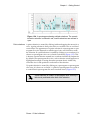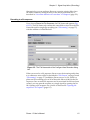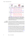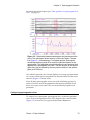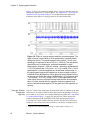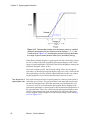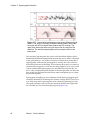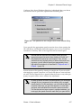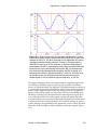
1
Raven 1.2 User’s Manual
Revision 1
10 November 2004
This manual can be printed or used online. To access all online features, we recommend viewing with the latest version of Adobe [Acrobat]
Reader, available free at http://www.acrobat.com. For online viewing,
use the bookmarks in the navigation pane on the left to navigate to sections within the manual. Cross references in the text and index entries
are hypertext links: click the link to view the referenced section or page.
Copyright notice
Raven software, the Raven 1.2 User’s Manual , and example sounds Copyright ©2003 Cornell Lab of Ornithology. All rights reserved. Reproduction of any part of this work in any form without permission is prohibited.
The Raven software includes code licensed from RSA Security, Inc. Some portions licensed from IBM are
available at http://oss.software.ibm.com/icu4j/.
Trademarks
Microsoft and Windows are registered trademarks of Microsoft Corporation in the United States and/or
other countries. Mac and Mac OS are registered trademarks of Apple Computer, Inc. PostScript is a registered trademark of Adobe Systems, Inc. Java is a registered trademark of Sun Microsystems, Inc. Other
brands are trademarks of their respective holders and should be noted as such.
Mention of specific software or hardware products in this manual is for informational purposes only and
does not imply endorsement or recommendation of any product. Cornell University and the Cornell Lab
of Ornithology make no claims regarding the performance of these products.
Credits
Raven was developed with partial support from the US National Science Foundation (grant
DBI-9876714, Principal Investigators: Christopher W. Clark and Kurt M. Fristrup), with additional support
from the Cornell Lab of Ornithology.
Raven was written by Harold Mills, Tim Krein, Scott Maher, Christina Ahrens, Jason Rohrer, and
Jason Adaska.
The Raven User’s Manual was written by Russell A. Charif with contributions by Wendy Alberg.
Raven artwork by Diane Tessaglia-Hymes.
The Raven development project is under the general direction of Christopher W. Clark and
Kurt M. Fristrup.
Citation
When citing use of Raven in scientific publications, please refer to this manual as follows:
Charif, RA, CW Clark, and KM Fristrup. 2004. Raven 1.2 User’s Manual. Cornell Laboratory of
Ornithology, Ithaca, NY.
For more information about Raven, visit the Raven website: www.birds.cornell.edu/raven
Bioacoustics Research Program
Cornell Lab of Ornithology
159 Sapsucker Woods Rd.
Ithaca, NY 14850
USA
Raven 1.2 User’s Manual, revision 1
Contents
About This Manual . . . . . . . . . . . . . . . . . . . . . . . . . . . . ix
Typographical conventions . . . . . . . . . . . . . . . . . . . . . . . . . . . . . . . . . . . . . . . . . . .ix
Fonts . . . . . . . . . . . . . . . . . . . . . . . . . . . . . . . . . . . . . . . . . . . . . . . . . . . . . . . . . . . . ix
Menu commands. . . . . . . . . . . . . . . . . . . . . . . . . . . . . . . . . . . . . . . . . . . . . . . . . . . ix
Cross-reference links . . . . . . . . . . . . . . . . . . . . . . . . . . . . . . . . . . . . . . . . . . . . . . . ix
Boxed notes. . . . . . . . . . . . . . . . . . . . . . . . . . . . . . . . . . . . . . . . . . . . . . . . . . . . . . . . . . . . . . . . . . . . . . . . . ix
Contextual menus . . . . . . . . . . . . . . . . . . . . . . . . . . . . . . . . . . . . . . . . . . . . . . . . . . . x
Keyboard shortcuts and menu mnemonics . . . . . . . . . . . . . . . . . . . . . . . . . . . . . x
Your feedback and updates to this manual . . . . . . . . . . . . . . . . . . . . . . . . . . . . .xi
Chapter 1 Getting Started with Raven. . . . . . . . . . . . . . . . . . . . . . .1
About this chapter. . . . . . . . . . . . . . . . . . . . . . . . . . . . . . . . . . . . . . . . . . . . . . . . . . . 1
Opening a sound file . . . . . . . . . . . . . . . . . . . . . . . . . . . . . . . . . . . . . . . . . . . . . . . . 1
The Raven window . . . . . . . . . . . . . . . . . . . . . . . . . . . . . . . . . . . . . . . . . . . . . . . . . . 4
The sound window . . . . . . . . . . . . . . . . . . . . . . . . . . . . . . . . . . . . . . . . . . . . . . . . .
The active view . . . . . . . . . . . . . . . . . . . . . . . . . . . . . . . . . . . . . . . . . . . . . . . . . . . .
Spectrogram brightness and contrast . . . . . . . . . . . . . . . . . . . . . . . . . . . . . . . . . . .
Moving and resizing a sound window . . . . . . . . . . . . . . . . . . . . . . . . . . . . . . . . . . .
The side panel. . . . . . . . . . . . . . . . . . . . . . . . . . . . . . . . . . . . . . . . . . . . . . . . . . . . .
5
7
7
8
8
Playing a sound . . . . . . . . . . . . . . . . . . . . . . . . . . . . . . . . . . . . . . . . . . . . . . . . . . . . . 8
Playing a selected part of a signal. . . . . . . . . . . . . . . . . . . . . . . . . . . . . . . . . . . . . . 9
Position markers and scrolling playback . . . . . . . . . . . . . . . . . . . . . . . . . . . . . . . . . 9
Playback rate. . . . . . . . . . . . . . . . . . . . . . . . . . . . . . . . . . . . . . . . . . . . . . . . . . . . . 10
Changing the position and scale of a view (zooming). . . . . . . . . . . . . . . . . . . 10
Position of a view . . . . . . . . . . . . . . . . . . . . . . . . . . . . . . . . . . . . . . . . . . . . . . . . .
Position markers . . . . . . . . . . . . . . . . . . . . . . . . . . . . . . . . . . . . . . . . . . . . . . .
Position vs. position location . . . . . . . . . . . . . . . . . . . . . . . . . . . . . . . . . . . . . .
Scrollbars . . . . . . . . . . . . . . . . . . . . . . . . . . . . . . . . . . . . . . . . . . . . . . . . . . . . .
Scale of a view . . . . . . . . . . . . . . . . . . . . . . . . . . . . . . . . . . . . . . . . . . . . . . . . . . .
Using zoom buttons to change scale . . . . . . . . . . . . . . . . . . . . . . . . . . . . . . . . . .
Zoom to selection . . . . . . . . . . . . . . . . . . . . . . . . . . . . . . . . . . . . . . . . . . . . . . . . .
Zoom to entire axis . . . . . . . . . . . . . . . . . . . . . . . . . . . . . . . . . . . . . . . . . . . . . . . .
10
10
13
13
14
14
16
16
Making a spectrogram slice. . . . . . . . . . . . . . . . . . . . . . . . . . . . . . . . . . . . . . . . . . 17
Linkage between spectrogram and spectrogram slice views . . . . . . . . . . . . . . . . 19
Unlinking and linking views . . . . . . . . . . . . . . . . . . . . . . . . . . . . . . . . . . . . . . . . 20
Unlinking a view via the contextual menu . . . . . . . . . . . . . . . . . . . . . . . . . . . . . . .
Restoring or creating new linkages . . . . . . . . . . . . . . . . . . . . . . . . . . . . . . . . . . .
Creating a new linkage group . . . . . . . . . . . . . . . . . . . . . . . . . . . . . . . . . . . . . . . .
Other linkable properties . . . . . . . . . . . . . . . . . . . . . . . . . . . . . . . . . . . . . . . . . . . .
20
21
23
23
Controlling how views are displayed . . . . . . . . . . . . . . . . . . . . . . . . . . . . . . . . 23
Hiding and showing views . . . . . . . . . . . . . . . . . . . . . . . . . . . . . . . . . . . . . . . . . . . 23
Deleting a view . . . . . . . . . . . . . . . . . . . . . . . . . . . . . . . . . . . . . . . . . . . . . . . . . . . 24
Raven 1.2 User’s Manual
i
Changing the order in which views are displayed . . . . . . . . . . . . . . . . . . . . . . . . . 24
Hiding and showing window components . . . . . . . . . . . . . . . . . . . . . . . . . . . . . . . 25
Selections and measurements. . . . . . . . . . . . . . . . . . . . . . . . . . . . . . . . . . . . . . . . 26
About selections . . . . . . . . . . . . . . . . . . . . . . . . . . . . . . . . . . . . . . . . . . . . . . . . . .
Creating and modifying range selections . . . . . . . . . . . . . . . . . . . . . . . . . . . . . . .
Selection control points . . . . . . . . . . . . . . . . . . . . . . . . . . . . . . . . . . . . . . . . . .
Committed vs. uncommitted selections . . . . . . . . . . . . . . . . . . . . . . . . . . . . . .
The active selection . . . . . . . . . . . . . . . . . . . . . . . . . . . . . . . . . . . . . . . . . . . . .
Point selections . . . . . . . . . . . . . . . . . . . . . . . . . . . . . . . . . . . . . . . . . . . . . . . . . . .
Deactivating and clearing selections . . . . . . . . . . . . . . . . . . . . . . . . . . . . . . . . . . .
The Selection Table . . . . . . . . . . . . . . . . . . . . . . . . . . . . . . . . . . . . . . . . . . . . . . .
Choosing measurements to display . . . . . . . . . . . . . . . . . . . . . . . . . . . . . . . . . . .
Annotations . . . . . . . . . . . . . . . . . . . . . . . . . . . . . . . . . . . . . . . . . . . . . . . . . . . . . .
Saving the selection table to a text file . . . . . . . . . . . . . . . . . . . . . . . . . . . . . . . . .
26
27
27
28
28
29
30
30
32
33
33
Editing a sound . . . . . . . . . . . . . . . . . . . . . . . . . . . . . . . . . . . . . . . . . . . . . . . . . . . . 34
Cut, Copy, Paste, and Delete . . . . . . . . . . . . . . . . . . . . . . . . . . . . . . . . . . . . . . . . 34
Undoing changes . . . . . . . . . . . . . . . . . . . . . . . . . . . . . . . . . . . . . . . . . . . . . . . . . 35
Filtering and amplifying sounds. . . . . . . . . . . . . . . . . . . . . . . . . . . . . . . . . . . . . . . 35
Color schemes . . . . . . . . . . . . . . . . . . . . . . . . . . . . . . . . . . . . . . . . . . . . . . . . . . . . . 36
Spectrogram colormaps . . . . . . . . . . . . . . . . . . . . . . . . . . . . . . . . . . . . . . . . . . . . 36
Editing color schemes . . . . . . . . . . . . . . . . . . . . . . . . . . . . . . . . . . . . . . . . . . . . . . 37
Multiple-line views. . . . . . . . . . . . . . . . . . . . . . . . . . . . . . . . . . . . . . . . . . . . . . . . . 37
Grouping views with multiple lines . . . . . . . . . . . . . . . . . . . . . . . . . . . . . . . . . . . . 38
Working with more than one sound . . . . . . . . . . . . . . . . . . . . . . . . . . . . . . . . . . 40
Using sound window presets . . . . . . . . . . . . . . . . . . . . . . . . . . . . . . . . . . . . . . . . 41
Saving and retrieving your work . . . . . . . . . . . . . . . . . . . . . . . . . . . . . . . . . . . . . 43
Saving a signal . . . . . . . . . . . . . . . . . . . . . . . . . . . . . . . . . . . . . . . . . . . . . . . . . . . 43
Saving and opening workspaces. . . . . . . . . . . . . . . . . . . . . . . . . . . . . . . . . . . . . . 44
Printing and exporting images . . . . . . . . . . . . . . . . . . . . . . . . . . . . . . . . . . . . . . . 44
Printing . . . . . . . . . . . . . . . . . . . . . . . . . . . . . . . . . . . . . . . . . . . . . . . . . . . . . . . . . 44
Exporting images to files . . . . . . . . . . . . . . . . . . . . . . . . . . . . . . . . . . . . . . . . . . . . 45
Copying images to the clipboard . . . . . . . . . . . . . . . . . . . . . . . . . . . . . . . . . . . . . . 45
Recording a sound (acquiring input) . . . . . . . . . . . . . . . . . . . . . . . . . . . . . . . . . 45
Selecting an audio input device. . . . . . . . . . . . . . . . . . . . . . . . . . . . . . . . . . . . . . .
The Configure New Recorder dialog box . . . . . . . . . . . . . . . . . . . . . . . . . . . . . . .
The Recorder Window. . . . . . . . . . . . . . . . . . . . . . . . . . . . . . . . . . . . . . . . . . . . . .
Starting and stopping the real-time signal display. . . . . . . . . . . . . . . . . . . . . . . . .
Displaying real-time spectrograms and spectrogram slices . . . . . . . . . . . . . . . . .
Other operations while recording . . . . . . . . . . . . . . . . . . . . . . . . . . . . . . . . . . . . .
While recording is stopped… . . . . . . . . . . . . . . . . . . . . . . . . . . . . . . . . . . . . . . . .
More about recording . . . . . . . . . . . . . . . . . . . . . . . . . . . . . . . . . . . . . . . . . . . . . .
45
46
46
47
47
48
48
48
Contacting the Raven development and support team . . . . . . . . . . . . . . . . . . 48
Chapter 2 Signal Acquisition (Recording) . . . . . . . . . . . . . . . . . .51
About this chapter. . . . . . . . . . . . . . . . . . . . . . . . . . . . . . . . . . . . . . . . . . . . . . . . . . 51
Overview of signal acquisition. . . . . . . . . . . . . . . . . . . . . . . . . . . . . . . . . . . . . . . 51
Recording modes . . . . . . . . . . . . . . . . . . . . . . . . . . . . . . . . . . . . . . . . . . . . . . . . . 51
Creating a recorder . . . . . . . . . . . . . . . . . . . . . . . . . . . . . . . . . . . . . . . . . . . . . . . . 52
ii
Raven 1.2 User’s Manual
Recording Input. . . . . . . . . . . . . . . . . . . . . . . . . . . . . . . . . . . . . . . . . . . . . . . . . . . . 52
Device . . . . . . . . . . . . . . . . . . . . . . . . . . . . . . . . . . . . . . . . . . . . . . . . . . . . . . . . . .
Sample Rate . . . . . . . . . . . . . . . . . . . . . . . . . . . . . . . . . . . . . . . . . . . . . . . . . . . . .
Channels . . . . . . . . . . . . . . . . . . . . . . . . . . . . . . . . . . . . . . . . . . . . . . . . . . . . . . . .
Sample Format . . . . . . . . . . . . . . . . . . . . . . . . . . . . . . . . . . . . . . . . . . . . . . . . . . .
52
53
53
53
Recording Display. . . . . . . . . . . . . . . . . . . . . . . . . . . . . . . . . . . . . . . . . . . . . . . . . . 54
Buffer Size. . . . . . . . . . . . . . . . . . . . . . . . . . . . . . . . . . . . . . . . . . . . . . . . . . . . . . .
Update Rate . . . . . . . . . . . . . . . . . . . . . . . . . . . . . . . . . . . . . . . . . . . . . . . . . . . . .
Latency . . . . . . . . . . . . . . . . . . . . . . . . . . . . . . . . . . . . . . . . . . . . . . . . . . . . . . . . .
Display latency vs. processing latency. . . . . . . . . . . . . . . . . . . . . . . . . . . . . . .
Window preset. . . . . . . . . . . . . . . . . . . . . . . . . . . . . . . . . . . . . . . . . . . . . . . . . . . .
54
54
55
55
55
File Format . . . . . . . . . . . . . . . . . . . . . . . . . . . . . . . . . . . . . . . . . . . . . . . . . . . . . . . . 56
File Format . . . . . . . . . . . . . . . . . . . . . . . . . . . . . . . . . . . . . . . . . . . . . . . . . . . . . . 56
Sample Size . . . . . . . . . . . . . . . . . . . . . . . . . . . . . . . . . . . . . . . . . . . . . . . . . . . . . 57
File Size. . . . . . . . . . . . . . . . . . . . . . . . . . . . . . . . . . . . . . . . . . . . . . . . . . . . . . . . . 57
File naming . . . . . . . . . . . . . . . . . . . . . . . . . . . . . . . . . . . . . . . . . . . . . . . . . . . . . . . . 57
Directory . . . . . . . . . . . . . . . . . . . . . . . . . . . . . . . . . . . . . . . . . . . . . . . . . . . . . . . .
Sound File(s) . . . . . . . . . . . . . . . . . . . . . . . . . . . . . . . . . . . . . . . . . . . . . . . . . . . . .
Start Time . . . . . . . . . . . . . . . . . . . . . . . . . . . . . . . . . . . . . . . . . . . . . . . . . . . . . . .
File name collisions . . . . . . . . . . . . . . . . . . . . . . . . . . . . . . . . . . . . . . . . . . . . . . . .
58
58
60
60
Recording to a file sequence . . . . . . . . . . . . . . . . . . . . . . . . . . . . . . . . . . . . . . . . . 61
Using recorder presets . . . . . . . . . . . . . . . . . . . . . . . . . . . . . . . . . . . . . . . . . . . . . . 62
The recorder window: real-time views during recording . . . . . . . . . . . . . . . 63
Creating real-time signal views . . . . . . . . . . . . . . . . . . . . . . . . . . . . . . . . . . . . . . .
Recording to memory . . . . . . . . . . . . . . . . . . . . . . . . . . . . . . . . . . . . . . . . . . . . . .
Recording to files. . . . . . . . . . . . . . . . . . . . . . . . . . . . . . . . . . . . . . . . . . . . . . . . . .
Retroactive recording to files. . . . . . . . . . . . . . . . . . . . . . . . . . . . . . . . . . . . . . . . .
Adjusting recording level . . . . . . . . . . . . . . . . . . . . . . . . . . . . . . . . . . . . . . . . . . . .
Navigating and selecting data in a running recorder . . . . . . . . . . . . . . . . . . . . . . .
Zooming and scrolling . . . . . . . . . . . . . . . . . . . . . . . . . . . . . . . . . . . . . . . . . . .
Selections and editing in a recorder window . . . . . . . . . . . . . . . . . . . . . . . . . .
Reconfiguring an existing recorder . . . . . . . . . . . . . . . . . . . . . . . . . . . . . . . . . . . .
Reconfiguring while acquisition is stopped . . . . . . . . . . . . . . . . . . . . . . . . . . .
Reconfiguring while recording . . . . . . . . . . . . . . . . . . . . . . . . . . . . . . . . . . . . .
Multiple recorder windows. . . . . . . . . . . . . . . . . . . . . . . . . . . . . . . . . . . . . . . . . . .
63
64
64
64
65
66
66
67
67
67
67
67
Advanced options: acquiring from recordings at altered input speeds . . . . 67
Advanced options: sample rate conversion during recording . . . . . . . . . . . . 69
Why decimation is useful. . . . . . . . . . . . . . . . . . . . . . . . . . . . . . . . . . . . . . . . . . . . 69
Decimation Factor . . . . . . . . . . . . . . . . . . . . . . . . . . . . . . . . . . . . . . . . . . . . . . . . . 70
Advanced options: scheduled recording . . . . . . . . . . . . . . . . . . . . . . . . . . . . . . 70
Retroactive Recording Offset . . . . . . . . . . . . . . . . . . . . . . . . . . . . . . . . . . . . . . . . 71
Problems with recording . . . . . . . . . . . . . . . . . . . . . . . . . . . . . . . . . . . . . . . . . . . . 71
Device unavailable . . . . . . . . . . . . . . . . . . . . . . . . . . . . . . . . . . . . . . . . . . . . . . . . 71
Unsupported audio format. . . . . . . . . . . . . . . . . . . . . . . . . . . . . . . . . . . . . . . . . . . 71
Chapter 3 Spectrographic Analysis . . . . . . . . . . . . . . . . . . . . . . . .73
About this chapter. . . . . . . . . . . . . . . . . . . . . . . . . . . . . . . . . . . . . . . . . . . . . . . . . . 73
About spectrographic views . . . . . . . . . . . . . . . . . . . . . . . . . . . . . . . . . . . . . . . . . 73
Raven 1.2 User’s Manual
iii
How the spectrographic views are related . . . . . . . . . . . . . . . . . . . . . . . . . . . . . . 74
Configuring spectrographic views. . . . . . . . . . . . . . . . . . . . . . . . . . . . . . . . . . . . 75
Window type . . . . . . . . . . . . . . . . . . . . . . . . . . . . . . . . . . . . . . . . . . . . . . . . . . . . .
Window size . . . . . . . . . . . . . . . . . . . . . . . . . . . . . . . . . . . . . . . . . . . . . . . . . . . . .
Window Size slider control . . . . . . . . . . . . . . . . . . . . . . . . . . . . . . . . . . . . . . . .
Beta (Kaiser window only). . . . . . . . . . . . . . . . . . . . . . . . . . . . . . . . . . . . . . . . . . .
3 dB Bandwidth . . . . . . . . . . . . . . . . . . . . . . . . . . . . . . . . . . . . . . . . . . . . . . . . . . .
Choosing the window size. . . . . . . . . . . . . . . . . . . . . . . . . . . . . . . . . . . . . . . . . . .
Time grid: Window Overlap and
Hop Size . . . . . . . . . . . . . . . . . . . . . . . . . . . . . . . . . . . . . . . . . . . . . . . . . . . . . . . . . . . . . . . . . . . . . . . . . .
Lock Overlap vs. Lock Hop Size . . . . . . . . . . . . . . . . . . . . . . . . . . . . . . . . . . .
Frequency grid spacing and DFT size. . . . . . . . . . . . . . . . . . . . . . . . . . . . . . . . . .
Lock DFT Size . . . . . . . . . . . . . . . . . . . . . . . . . . . . . . . . . . . . . . . . . . . . . . . . .
Spectrum averaging . . . . . . . . . . . . . . . . . . . . . . . . . . . . . . . . . . . . . . . . . . . . . . .
Apply and Auto-apply . . . . . . . . . . . . . . . . . . . . . . . . . . . . . . . . . . . . . . . . . . . . . .
Spectrogram presets . . . . . . . . . . . . . . . . . . . . . . . . . . . . . . . . . . . . . . . . . . . . . . .
76
79
80
80
80
81
82
84
84
85
85
87
88
Spectrogram views . . . . . . . . . . . . . . . . . . . . . . . . . . . . . . . . . . . . . . . . . . . . . . . . . 88
Significance of the color (grayscale) values . . . . . . . . . . . . . . . . . . . . . . . . . . . . .
Brightness and contrast. . . . . . . . . . . . . . . . . . . . . . . . . . . . . . . . . . . . . . . . . . . . .
Time alignment of spectrogram data. . . . . . . . . . . . . . . . . . . . . . . . . . . . . . . . . . .
Smoothed vs. unsmoothed display . . . . . . . . . . . . . . . . . . . . . . . . . . . . . . . . . . . .
88
88
90
92
Spectrogram slice views. . . . . . . . . . . . . . . . . . . . . . . . . . . . . . . . . . . . . . . . . . . . . 95
Time position of a spectrogram slice view. . . . . . . . . . . . . . . . . . . . . . . . . . . . . . . 95
Significance of the spectrum values . . . . . . . . . . . . . . . . . . . . . . . . . . . . . . . . . . . 96
Selection spectrum views . . . . . . . . . . . . . . . . . . . . . . . . . . . . . . . . . . . . . . . . . . . 97
Significance of the spectrum values . . . . . . . . . . . . . . . . . . . . . . . . . . . . . . . . . . . 97
Changing parameters for an existing spectrographic view. . . . . . . . . . . . . . . 97
Chapter 4 Selections and Measurements . . . . . . . . . . . . . . . . . . .99
About this chapter. . . . . . . . . . . . . . . . . . . . . . . . . . . . . . . . . . . . . . . . . . . . . . . . . . 99
Annotations . . . . . . . . . . . . . . . . . . . . . . . . . . . . . . . . . . . . . . . . . . . . . . . . . . . . . . . 99
Creating, renaming, and deleting annotation columns . . . . . . . . . . . . . . . . . . . .
Entering annotations . . . . . . . . . . . . . . . . . . . . . . . . . . . . . . . . . . . . . . . . . . . . . .
Entering annotations when committing selections . . . . . . . . . . . . . . . . . . . . .
Entering annotations directly in the selection table . . . . . . . . . . . . . . . . . . . .
Using the Annotate Selection command . . . . . . . . . . . . . . . . . . . . . . . . . . . .
100
100
100
101
101
Creating selections in multi-channel sounds . . . . . . . . . . . . . . . . . . . . . . . . . 101
Configuring the selection table . . . . . . . . . . . . . . . . . . . . . . . . . . . . . . . . . . . . . 102
Measurement precision and format. . . . . . . . . . . . . . . . . . . . . . . . . . . . . . . . . . .
Using measurement presets . . . . . . . . . . . . . . . . . . . . . . . . . . . . . . . . . . . . . . . .
Visibility of view and channel entries. . . . . . . . . . . . . . . . . . . . . . . . . . . . . . . . . .
Sort order of view and channel entries . . . . . . . . . . . . . . . . . . . . . . . . . . . . . . . .
Renumbering selections . . . . . . . . . . . . . . . . . . . . . . . . . . . . . . . . . . . . . . . . . . .
102
103
104
104
105
Working with selections . . . . . . . . . . . . . . . . . . . . . . . . . . . . . . . . . . . . . . . . . . . 105
Activating a selection from the selection table . . . . . . . . . . . . . . . . . . . . . . . . . .
Finding the active selection . . . . . . . . . . . . . . . . . . . . . . . . . . . . . . . . . . . . . . . . .
Modifying selection bounds . . . . . . . . . . . . . . . . . . . . . . . . . . . . . . . . . . . . . . . . .
Moving selection control points . . . . . . . . . . . . . . . . . . . . . . . . . . . . . . . . . . .
Editing in the selection table . . . . . . . . . . . . . . . . . . . . . . . . . . . . . . . . . . . . .
iv
Raven 1.2 User’s Manual
105
105
106
106
106
Using the Selection tab in the side panel . . . . . . . . . . . . . . . . . . . . . . . . . . . .
Modifying selection channels . . . . . . . . . . . . . . . . . . . . . . . . . . . . . . . . . . . . . . .
Selection tables in paged sound windows. . . . . . . . . . . . . . . . . . . . . . . . . . . . . .
Saving the active selection . . . . . . . . . . . . . . . . . . . . . . . . . . . . . . . . . . . . . . . . .
Copying selected rows from the selection table . . . . . . . . . . . . . . . . . . . . . . . . .
Clearing selections . . . . . . . . . . . . . . . . . . . . . . . . . . . . . . . . . . . . . . . . . . . . . . .
106
107
107
107
107
108
Copying, pasting, and cloning selection boundaries . . . . . . . . . . . . . . . . . . . 108
Creating duplicate selections at different times. . . . . . . . . . . . . . . . . . . . . . . . . . 109
Cloning selections . . . . . . . . . . . . . . . . . . . . . . . . . . . . . . . . . . . . . . . . . . . . . . . . 109
Using cloning to segment a sound . . . . . . . . . . . . . . . . . . . . . . . . . . . . . . . . . 109
Selection labels . . . . . . . . . . . . . . . . . . . . . . . . . . . . . . . . . . . . . . . . . . . . . . . . . . . 109
Saving and retrieving selections . . . . . . . . . . . . . . . . . . . . . . . . . . . . . . . . . . . . 110
Format of selection files . . . . . . . . . . . . . . . . . . . . . . . . . . . . . . . . . . . . . . . . . . . 111
Measurements . . . . . . . . . . . . . . . . . . . . . . . . . . . . . . . . . . . . . . . . . . . . . . . . . . . . 111
Chapter 5 Advanced Raven Usage . . . . . . . . . . . . . . . . . . . . . . .115
About this chapter. . . . . . . . . . . . . . . . . . . . . . . . . . . . . . . . . . . . . . . . . . . . . . . . . 115
Opening multiple sound files in separate windows . . . . . . . . . . . . . . . . . . . 115
Opening file sequences . . . . . . . . . . . . . . . . . . . . . . . . . . . . . . . . . . . . . . . . . . . . 117
Using a list file . . . . . . . . . . . . . . . . . . . . . . . . . . . . . . . . . . . . . . . . . . . . . . . . . . . 117
Format of a list file . . . . . . . . . . . . . . . . . . . . . . . . . . . . . . . . . . . . . . . . . . . . . 118
Selecting files in a sequence individually . . . . . . . . . . . . . . . . . . . . . . . . . . . . . . 119
Paged sound windows: opening large sounds . . . . . . . . . . . . . . . . . . . . . . . . 120
Configuring a new paged sound window. . . . . . . . . . . . . . . . . . . . . . . . . . . . . . .
Navigating through signals in paged sound windows . . . . . . . . . . . . . . . . . . . . .
The paging scrollbar. . . . . . . . . . . . . . . . . . . . . . . . . . . . . . . . . . . . . . . . . . . .
Moving the page incrementally: the Page and Step buttons . . . . . . . . . . . . .
Jumping directly to a particular time within a signal . . . . . . . . . . . . . . . . . . . .
The current file indicator; jumping to a particular file in a sequence . . . . . . .
Selections spanning pages . . . . . . . . . . . . . . . . . . . . . . . . . . . . . . . . . . . . . . . . .
Reconfiguring paging for an existing window . . . . . . . . . . . . . . . . . . . . . . . . . . .
120
121
122
123
123
123
123
123
Working with multi-channel sounds . . . . . . . . . . . . . . . . . . . . . . . . . . . . . . . . 124
Displaying and hiding channels. . . . . . . . . . . . . . . . . . . . . . . . . . . . . . . . . . . . . . 124
Editing multi-channel sounds . . . . . . . . . . . . . . . . . . . . . . . . . . . . . . . . . . . . . . . 125
Selecting channels for editing operations . . . . . . . . . . . . . . . . . . . . . . . . . . . 125
Correcting sounds acquired at altered speeds . . . . . . . . . . . . . . . . . . . . . . . . .
Setting the scale and position of view axes . . . . . . . . . . . . . . . . . . . . . . . . . . .
Creating linked spectrographic views. . . . . . . . . . . . . . . . . . . . . . . . . . . . . . . .
Filtering and amplifying sounds . . . . . . . . . . . . . . . . . . . . . . . . . . . . . . . . . . . .
126
128
128
128
Filtering . . . . . . . . . . . . . . . . . . . . . . . . . . . . . . . . . . . . . . . . . . . . . . . . . . . . . . . . 128
Amplifying . . . . . . . . . . . . . . . . . . . . . . . . . . . . . . . . . . . . . . . . . . . . . . . . . . . . . . 129
Editing color schemes. . . . . . . . . . . . . . . . . . . . . . . . . . . . . . . . . . . . . . . . . . . . . . 129
Choosing a color scheme element to edit . . . . . . . . . . . . . . . . . . . . . . . . . . . . . .
Choosing colors. . . . . . . . . . . . . . . . . . . . . . . . . . . . . . . . . . . . . . . . . . . . . . . . . .
Swatches color chooser . . . . . . . . . . . . . . . . . . . . . . . . . . . . . . . . . . . . . . . . .
HSB color chooser . . . . . . . . . . . . . . . . . . . . . . . . . . . . . . . . . . . . . . . . . . . . .
RGB color chooser. . . . . . . . . . . . . . . . . . . . . . . . . . . . . . . . . . . . . . . . . . . . .
Opacity . . . . . . . . . . . . . . . . . . . . . . . . . . . . . . . . . . . . . . . . . . . . . . . . . . . . . . . .
Raven 1.2 User’s Manual
132
132
132
133
133
134
v
Color scheme presets . . . . . . . . . . . . . . . . . . . . . . . . . . . . . . . . . . . . . . . . . . . . . 135
Auto-Apply, Apply, Reset, OK, and Close . . . . . . . . . . . . . . . . . . . . . . . . . . . . . . 135
The Preset Manager . . . . . . . . . . . . . . . . . . . . . . . . . . . . . . . . . . . . . . . . . . . . . . . 135
The Memory Manager . . . . . . . . . . . . . . . . . . . . . . . . . . . . . . . . . . . . . . . . . . . . . 137
About Raven memory allocation . . . . . . . . . . . . . . . . . . . . . . . . . . . . . . . . . . . . .
The Memory Manager window . . . . . . . . . . . . . . . . . . . . . . . . . . . . . . . . . . . . . .
Memory usage summary . . . . . . . . . . . . . . . . . . . . . . . . . . . . . . . . . . . . . . . .
Configuring Maximum Heap Size. . . . . . . . . . . . . . . . . . . . . . . . . . . . . . . . . .
The memory usage list. . . . . . . . . . . . . . . . . . . . . . . . . . . . . . . . . . . . . . . . . .
Reclaiming unused memory. . . . . . . . . . . . . . . . . . . . . . . . . . . . . . . . . . . . . .
138
139
139
139
139
140
Raven program and documentation updates. . . . . . . . . . . . . . . . . . . . . . . . . . 140
Chapter 6 Preferences:
Customizing Raven . . . . . . . . . . . . . . . . . . . . . . . . . . .143
About this chapter. . . . . . . . . . . . . . . . . . . . . . . . . . . . . . . . . . . . . . . . . . . . . . . . . 143
About Raven preferences. . . . . . . . . . . . . . . . . . . . . . . . . . . . . . . . . . . . . . . . . . . 143
The Raven preference file . . . . . . . . . . . . . . . . . . . . . . . . . . . . . . . . . . . . . . . . . . 143
Default presets . . . . . . . . . . . . . . . . . . . . . . . . . . . . . . . . . . . . . . . . . . . . . . . . . . . . 144
Spectrogram presets . . . . . . . . . . . . . . . . . . . . . . . . . . . . . . . . . . . . . . . . . . . . . .
Recorder presets. . . . . . . . . . . . . . . . . . . . . . . . . . . . . . . . . . . . . . . . . . . . . . . . .
Measurement presets . . . . . . . . . . . . . . . . . . . . . . . . . . . . . . . . . . . . . . . . . . . . .
Sound window presets . . . . . . . . . . . . . . . . . . . . . . . . . . . . . . . . . . . . . . . . . . . .
Color scheme presets . . . . . . . . . . . . . . . . . . . . . . . . . . . . . . . . . . . . . . . . . . . . .
145
145
146
146
146
Default workspace . . . . . . . . . . . . . . . . . . . . . . . . . . . . . . . . . . . . . . . . . . . . . . . . 147
Default directories. . . . . . . . . . . . . . . . . . . . . . . . . . . . . . . . . . . . . . . . . . . . . . . . . 148
Default measurement precision . . . . . . . . . . . . . . . . . . . . . . . . . . . . . . . . . . . . . 148
Time . . . . . . . . . . . . . . . . . . . . . . . . . . . . . . . . . . . . . . . . . . . . . . . . . . . . . . . . . .
Frequency . . . . . . . . . . . . . . . . . . . . . . . . . . . . . . . . . . . . . . . . . . . . . . . . . . . . . .
Amplitude . . . . . . . . . . . . . . . . . . . . . . . . . . . . . . . . . . . . . . . . . . . . . . . . . . . . . .
Power . . . . . . . . . . . . . . . . . . . . . . . . . . . . . . . . . . . . . . . . . . . . . . . . . . . . . . . . .
149
150
150
150
Overwrite behavior for recorders. . . . . . . . . . . . . . . . . . . . . . . . . . . . . . . . . . . . 151
Automatic updates . . . . . . . . . . . . . . . . . . . . . . . . . . . . . . . . . . . . . . . . . . . . . . . . 151
Email preferences . . . . . . . . . . . . . . . . . . . . . . . . . . . . . . . . . . . . . . . . . . . . . . . . . 151
Return address . . . . . . . . . . . . . . . . . . . . . . . . . . . . . . . . . . . . . . . . . . . . . . . . . . 151
Outgoing mail server . . . . . . . . . . . . . . . . . . . . . . . . . . . . . . . . . . . . . . . . . . . . . . 151
Appendix G Digital Representation of Sound . . . . . . . . . . . . . . . .153
About this appendix . . . . . . . . . . . . . . . . . . . . . . . . . . . . . . . . . . . . . . . . . . . . . . . 153
Digital sampling . . . . . . . . . . . . . . . . . . . . . . . . . . . . . . . . . . . . . . . . . . . . . . . . . . 153
Sampling rate . . . . . . . . . . . . . . . . . . . . . . . . . . . . . . . . . . . . . . . . . . . . . . . . . . . . . 154
Aliasing and the Nyquist frequency . . . . . . . . . . . . . . . . . . . . . . . . . . . . . . . . . . . 154
Sample size (amplitude resolution). . . . . . . . . . . . . . . . . . . . . . . . . . . . . . . . . . 157
Specifying sample sizes when acquiring and saving signals . . . . . . . . . . . . . . . 158
Storage requirements. . . . . . . . . . . . . . . . . . . . . . . . . . . . . . . . . . . . . . . . . . . . . . 158
vi
Raven 1.2 User’s Manual
Appendix H A Biologist’s Introduction to
Spectrum Analysis . . . . . . . . . . . . . . . . . . . . . . . . . . . .161
About this appendix . . . . . . . . . . . . . . . . . . . . . . . . . . . . . . . . . . . . . . . . . . . . . . . 161
What sound is. . . . . . . . . . . . . . . . . . . . . . . . . . . . . . . . . . . . . . . . . . . . . . . . . . . . . 161
Time domain and frequency domain representations of sound . . . . . . . . . 162
Spectral analysis of time-varying signals: spectrograms and STFT analysis .
165
Record length, bandwidth, and the time-frequency uncertainty principle 166
Making spectrograms . . . . . . . . . . . . . . . . . . . . . . . . . . . . . . . . . . . . . . . . . . . . . . 168
Analysis resolution and the time-frequency uncertainty principle . . . . . . . . . . . .
Time grid spacing and window overlap . . . . . . . . . . . . . . . . . . . . . . . . . . . . . . . .
Frequency grid spacing and DFT size. . . . . . . . . . . . . . . . . . . . . . . . . . . . . . . . .
Spectral smearing and sidelobes . . . . . . . . . . . . . . . . . . . . . . . . . . . . . . . . . . . .
Window functions . . . . . . . . . . . . . . . . . . . . . . . . . . . . . . . . . . . . . . . . . . . . . . . .
169
171
172
173
175
For further reading . . . . . . . . . . . . . . . . . . . . . . . . . . . . . . . . . . . . . . . . . . . . . . . . 177
Appendix I Configuring Audio Input . . . . . . . . . . . . . . . . . . . . . .179
About this appendix . . . . . . . . . . . . . . . . . . . . . . . . . . . . . . . . . . . . . . . . . . . . . . . 179
Windows 98, 2000, and XP . . . . . . . . . . . . . . . . . . . . . . . . . . . . . . . . . . . . . . . . . . 179
Mac OS X. . . . . . . . . . . . . . . . . . . . . . . . . . . . . . . . . . . . . . . . . . . . . . . . . . . . . . . . . 181
Raven 1.2 User’s Manual
vii
viii
Raven 1.2 User’s Manual
About This Manual
This manual describes Raven 1.2, which runs on Windows and Mac OS X
computers. Raven’s appearance on the two operating systems is slightly
different. In most cases, the differences in appearance are cosmetic and
simply reflect different styles used for rendering windows, dialog boxes,
and other user interface items. In cases where the differences are merely
cosmetic, illustrations in this manual show screen shots either from the
Windows or the Mac OS version of Raven. In the few cases where there
are more significant differences in the content or layout of information in
windows or dialog boxes, illustrations are shown from both platforms.
Typographical conventions
Fonts Throughout the manual, an alternate font is used to identify named items
in the Raven user interface, such as menus, menu commands, and items in
dialog boxes. Example: “To delete a view, activate the view and choose
Delete from its contextual menu or from the View menu.”
Menu commands Menu commands are identified by the name of the menu, followed by >,
followed by the name of the command. Example: File > Save “Sound 1”.
Cross-reference Cross-references within the PDF text are in blue, and are hyperlinks: clicklinks ing a cross-reference when viewing the text in Adobe (Acrobat) or Adobe
(Acrobat) Reader will take you directly to the referenced place in the text.
To return to the referencing point in the text, click the Back button in the
Acrobat toolbar.
Boxed notes
Boxes like this supplement the main text by providing helpful
tips or calling your attention to specific points.
WINDOWS
Boxes like this provide information that is specific to
either the Windows or Mac OS version of Raven.
Raven 1.2 User’s Manual
ix
About This Manual
Contextual menus
This manual refers in many places to commands located on contextual
menus (or context menus). A contextual menu is a menu that is relevant to
the particular item identified by the location of the mouse pointer. Under
the Windows operating system, contextual menus are activated by rightclicking. Under Mac OS X, contextual menus are activated by holding
down the Ctrl key while clicking.
MAC OS
Any computer running Mac OS X can be equipped with
a third-party USB two-button mouse. A two-button
mouse provides access to contextual menus by rightclicking (in addition to use of the Ctrl key while clicking).
Keyboard shortcuts and menu mnemonics
There are two ways to use the keyboard (rather than the mouse) to activate menu commands. Some commands have single-keystroke equivalents or shortcuts, activated by pressing the <Ctrl> (Windows) or
<Command> (Mac OS) key and a single other key simultaneously. Keyboard shortcuts are shown in menus to the right of the command name
(Figure 1). Any menu command can also be chosen by using mnemonics. A
menu mnemonic consists of a sequence of two or more keystrokes in
which the first keystroke activates a particular menu; subsequent keystrokes choose particular items from within the menu. To activate a particular menu, press the <Alt> (Windows) or <Option> (Mac OS) key and the
first letter of the menu name simultaneously. To choose an item from the
menu once it’s activated, press the key corresponding to the underlined
letter in the item name. For example, to choose the Open Workspace...
command from the File menu (Figure 1), press <Alt-F><W> (Windows) or
<Option-F><W> (Mac OS).
x
Raven 1.2 User’s Manual
About This Manual
Figure 1File menu
Figure 1. The File menu, showing keyboard shortcuts and mnemonics.
Your feedback and updates to this manual
If you find errors in this manual or have suggestions for future editions,
please contact us at [email protected].
From time to time, we release revisions of the manual to correct errors and
make other improvements. To find out whether you have the latest version of the manual, and to download any updates, use Raven’s Check for
Updates feature, described in “Raven program and documentation
updates” in Chapter 5 (page 140).
Raven 1.2 User’s Manual
xi
About This Manual
xii
Raven 1.2 User’s Manual
Chapter 1
Getting Started with Raven
About this chapter
This chapter introduces the major features of Raven using some of the
sound files supplied with the program as examples. Many details of how
these features work are deferred until later chapters. We recommend that
you read this chapter at the computer and try the examples as they’re discussed. We assume you know how to browse for files on your computer,
and have installed Raven as discussed in the Raven README file.
In this chapter you’ll learn how to:
•open an existing sound file using Raven
•display waveform, spectrogram, and spectrogram slice views of a sound
•play all or part of a sound file
•hide, show and zoom views of a signal
•edit a recorded sound
•save your changes
•make and save measurements of a signal
•record new signals
Opening a sound file
Launch Raven by double-clicking on its icon. (Depending on how you
installed Raven, there may be an icon for it on your desktop, in your Start
menu (Windows), in your dock (Mac OS), or you may have to open the
Raven folder to find it.) The Raven window appears on your screen. To
open a sound file, choose File > Open Sound Files... , or type <Ctrl-O>
(Windows) or <Command-O> (Mac OS). You’ll see Raven’s Open Sound
Files dialog box (Figure 1.1, Figure 1.2).
Raven 1.2 User’s Manual
1
Chapter 1: Getting Started
Figure 1.1. Open Sound dialog--Mac
Figure 1.1. Raven’s Open Sound Files dialog box on a Mac OS computer
Figure 1.2. Open Dialog--Windows
Figure 1.2. Raven’s Open Sound Files dialog box on a Windows computer.
The Open Sound Files dialog box displays a scrolling list of the files and
directories in the current directory. The name of the current directory is
given at the top of the dialog box. If the current directory is not “Examples” in the Raven program directory find the Examples directory now.
(To move up in the file system hierarchy, click on the name of the current
directory and select another directory from the pull-down menu that
appears. To move down the hierarchy, double-click on the name of a
2
Raven 1.2 User’s Manual
Chapter 1: Getting Started
directory in the scrolling list of files and directories within the current
directory.)
WINDOWS
On Windows computers, the Audio File Format panel
on the right side of the Open Sound Files dialog box
displays information about the currently selected file.
Select the file named “ChestnutSidedWarbler.aif” in the Examples directory. Click the Open button, or double-click on the file’s name. The Configure New Sound Window dialog box appears (Figure 1.3). The
Configure New Sound Window dialog box allows you to choose a window preset that controls the layout of a sound window (discussed in
“Using sound window presets” on page 41), and to control how much of
the sound is loaded into Raven’s working memory at one time (see “Paged
sound windows: opening large sounds” in Chapter 5 (page 120)). For now,
click OK to accept the default settings. A sound window appears on the
Raven desktop (Figure 1.4). The title bar of the sound window shows a
sequential number (starting at 1) that Raven assigns to each sound you
open, and the name of the file.
Figure 1.3. Configure Sound Window dialog
Figure 1.3. The Configure New Sound Window dialog box.
Raven 1.2 User’s Manual
3
Chapter 1: Getting Started
When Raven is running, you can open any WAVE or AIFF
sound file by dragging its icon from an Explorer (Windows) or
Finder (Mac OS) window or from the desktop and “dropping”
the icon anywhere in the Raven window.
The Raven window
Raven’s menu bar appears just below the title bar of the Raven window on
Windows computers (Figure 1.4) and at the top of the screen on Mac OS
computers (Figure 1.5). The control toolbar contains controls for common
Raven operations. When you position the mouse pointer over a control in
the toolbar, a “tooltip” appears giving the name of the tool. On the left side
of the Raven window is the side panel. The side panel contains tools that let
you control various aspects of how signals are displayed and played back.
To the right is the Raven desktop, which can contain one or more sound
windows.
4
Raven 1.2 User’s Manual
Chapter 1: Getting Started
Figure 1.4. Raven window
Figure 1.4. The Raven window on a Windows computer, with one
sound window open.
The sound window By default, when you first open a sound file Raven shows you a sound window that contains two views of the sound (Figure 1.4, Figure 1.5). The waveform (upper) view displays an oscillogram, or graph of the sound showing
amplitude versus time. The spectrogram (lower) view represents time on
the horizontal axis, frequency on the vertical axis, and relative power at
each time and frequency as a color (by default grayscale) value. Spectrogram views are discussed further in Chapter 3, “Spectrographic Analysis”.
In addition to waveforms and spectrograms, Raven can also display spectrogram slice views of a signal, and selection spectrum views, which show
the average spectrum of a selected portion of a signal. Spectrogram slice
views and selection spectrum views are discussed in “Making a spectrogram slice” on page 17, and in Chapter 3, “Spectrographic Analysis”.
Chapter 6, “Preferences: Customizing Raven” explains how to configure
Raven to display combinations of views other than the default waveform
and spectrogram when a signal is first opened.
Raven 1.2 User’s Manual
5
Chapter 1: Getting Started
The units used on the axes are indicated in the lower left corner of each
view. In the waveform, the units are seconds (S) for the horizontal time
axis, and kilounits (kU) for the vertical amplitude axis. The “units” displayed on the vertical axis of a waveform view are the actual sample values in the signal, which are proportional to the sound pressure at the
microphone when the sound was recorded. In the spectrogram, the units
are seconds (S) for the horizontal time axis, and kilohertz (kHz) for the
vertical frequency axis.
Figure 1.5. Raven window-- Mac
Figure 1.5. The Raven window on a Mac OS computer, with one
sound window open.
At the scale of magnification shown, you can’t see individual cycles of
oscillation of the waveform; what you see is the envelope of the entire signal. Later in this chapter you’ll learn how to zoom in to see fine details of a
waveform.
As you move the mouse pointer over the waveform view, the time of the
pointer’s location and the amplitude of the waveform at that time are
shown in the mouse measurement field at the bottom of the Raven window
6
Raven 1.2 User’s Manual
Chapter 1: Getting Started
(Figure 1.4). Often, the time scale is so compressed that the number of
sample points represented exceeds the number of pixels in the window. In
this case, each pixel stands for multiple sample points, and the measurement display shows the minimum and maximum values of the samples
represented at the time of the mouse position (as in Figure 1.4 ). Later you
will see how to zoom in so that individual points can be represented accurately.
As you move the mouse pointer over the spectrogram view, the time and
frequency of the pointer’s location, and the relative power at that time and
frequency are shown in the mouse measurement field (Figure 1.5).
The active view Most commands, buttons and scroll bars that affect views apply only to
the active view. Only one view in a sound window can be active at any
given time. The active view is identified by a colored vertical view selection
button at its left edge. The name of the active view is also highlighted on
the side panel’s Layout tab. In Figure 1.4, the waveform is the active view;
in Figure 1.5, the spectrogram is the active view. To activate a view, click
on its view selection button or in its axis areas. You can also activate a
view by clicking on its name in the side panel’s Layout tab.
Although you can activate a view by clicking in the data
region (i.e., above and to the right of the axes), doing so will
create a selection. Selections are discussed in “Selections
and measurements” on page 26.
Spectrogram When a spectrogram view is active, the brightness and contrast controls
brightness and on Raven’s control toolbar become active too (Figure 1.6).
contrast
Figure 1.6. Bright/contrast sliders
Figure 1.6. Spectrogram brightness and contrast controls.
If your spectrogram looks too dark or light, or if it’s hard to pick the signal
out of the background, move the brightness and contrast sliders to achieve
the desired appearance of the spectrogram. The brightness control adjusts
the overall darkness of the spectrogram: for a grayscale spectrogram (the
default), sliding the control to the right lightens the display.
The contrast control adjusts the number of different color (by default,
grayscale) values that are shown in the spectrogram. In a grayscale spectrogram, moving the contrast slider all the way to the right makes the display black and white: all values below some threshold are assigned to
Raven 1.2 User’s Manual
7
Chapter 1: Getting Started
white and the rest become black. In this case, the threshold between black
and white is determined by the brightness control. With the contrast control all the way to the left Raven displays up to 200 shades of gray.
The box next to each control tells you what percent contrast or brightness
you’ve set. If you prefer, you can type a percentage number into a box
instead of moving the slider.
See “Brightness and contrast” in Chapter 3 (page 88), for a more detailed
explanation of how these controls work.
Moving and resizing The sound window’s title bar has controls for moving, resizing and closa sound window ing it (Figure 1.4, Figure 1.5). To move the window around, click and drag
on the title bar. To minimize it (to reduce the whole window to a short title
bar at the bottom of the Raven window), click on the Minimize icon in the
title bar. The appearance and location of the Minimize, Resize, and Close
icons depends on the operating system under which Raven is running
(Figure 1.4, Figure 1.5). Clicking on a minimized window expands it again.
Click on the Resize icon to maximize the window, making it fill the entire
Raven desktop. When the window is maximized, clicking the Resize icon
again restores it to its previous size and position. Clicking on the Close
icon closes the window; if you close it, you’ll have to reopen the sound file
again by choosing File > Open Sound Files... or by typing <Ctrl-O> (Windows) or <Command-O> (Mac OS). You can also resize the window by
clicking and dragging on an edge or corner of the window.
The side panel The left side of the Raven window holds the side panel, which contains four
tabs: Layout, Linkage, Selection, and Playback. By default, the side panel
opens to the Layout tab. The side panel is discussed later in this chapter
(see “Unlinking and linking views” on page 20, “Controlling how views
are displayed” on page 23, and “Multiple-line views” on page 37). For
now, notice that “Waveform 1” and “Spectrogram 1” have appeared in the
top half of the Layout tab and “Channel 1” in the bottom half. The checkmarks in the corresponding checkboxes tells you that the sound window
is now displaying channel 1 of a waveform and a spectrogram view.
You can resize the side panel by dragging the vertical separator bar
between the side panel and the Raven desktop. To hide the side panel,
click on the left-pointing arrow at the top (Windows) or bottom (Mac OS)
of the separator bar. To show the side panel when it’s hidden, click on the
right-pointing arrow at the top of the separator bar at the left edge of the
Raven desktop. If the sound window is maximized when you hide the
side panel, it automatically expands to occupy the entire Raven desktop.
Playing a sound
The right-hand end of the control toolbar contains the playback controls
(Figure 1.7). To play back the part of the signal that is visible in the window, click the Play button, or press <Ctrl-Shift-P> (Windows) or <Command-Shift-P> (Mac OS).
8
Raven 1.2 User’s Manual
Chapter 1: Getting Started
Figure 1.7. Playback controls
Figure 1.7. The playback controls.
As the sound plays, a vertical green line, the playback cursor, moves across
the waveform from left to right to show you what part of the signal you
are hearing. To stop playing at any time, click the Stop button. When the
selection finishes playing, or when you click Stop, the playback cursor disappears.
Playing a selected You can select a portion of a signal to play: click and drag from one side to
part of a signal the other of the part of the signal you want to listen to, in either the waveform or spectrogram view. Raven marks your selection with a colored
rectangle. Click the Play button to play it.
Position markers The magenta vertical line at the left-hand edge of the waveform view is
and scrolling the time axis position marker. Each view in a sound window has two posiplayback tion markers, which identify unique locations along the horizontal and
vertical axes. Position markers are important for several types of Raven
operations, and are discussed further in “Changing the position and scale
of a view (zooming)” on page 10.
Using the mouse, grab the time axis position marker in either the waveform or spectrogram view and move it slightly away from the left edge of
the window (Figure 1.8). Click the Scrolling Play button to play the signal.
In scrolling playback, the signal view scrolls from right to left beneath the
position marker, like tape moving past the playback head of a tape
recorder. The position marker identifies the point in time that you are
hearing.
Raven 1.2 User’s Manual
9
Chapter 1: Getting Started
Figure 1.8 sound window, pos marker moved.
Figure 1.8. The ChestnutSidedWarbler sound window shown in Figure
1.4, with the time axis position marker moved away from the left edge of
the window.
During scrolling playback, you can drag the scroll thumb to move the signal so that a particular point of interest is at the time position marker. The
sound stops playing while you drag the scroll thumb and resumes immediately at the new time position when you release the scroll thumb.
Playback rate You can speed up or slow down the playback rate of the signal. By default
the playback rate is set at 1.0, or the same as the recording rate. Slowing
down the rate makes the sound lower in pitch and slower; speeding it up
makes it higher in pitch and faster. Try it now: type a number greater than
1 in the rate box to speed up or a decimal number between 0 and 1 to slow
down, press <Enter>, and then play the sound again.
Changing the position and scale of a view (zooming)
Position of a view Position markers
Each view that Raven displays has a horizontal and a vertical position associated with it, shown by a magenta line, known as a position marker. You
have already seen how the time position marker in a waveform view indi-
10
Raven 1.2 User’s Manual
Chapter 1: Getting Started
cates the current time during scrolling play (“Position markers and scrolling playback” on page 9).
When we speak of the “horizontal position marker” we mean
the line that marks the horizontal position, which is a vertical
line.
You can move the horizontal or vertical position marker of a view relative
to the window by grabbing it with the mouse and dragging it. To move a
particular point in the data shown in a view to the horizontal or vertical
center of the view pane, place the position marker on the point of interest,
then click the corresponding Center Position button (Figure 1.9). The position marker and the underlying data will jump to the center of the view
pane. Blue labels along the axes show the exact numeric values of the current horizontal and vertical positions.
WINDOWS
On computers running the Windows operating system,
you can make a view’s horizontal position marker jump
directly to a point by control-clicking at that point.
Figure 1.9. Center position buttons
Figure 1.9. The horizontal and vertical Center Position buttons.
Notice that when you move the time position of either the waveform or
spectrogram, the time position marker in the other view moves with it.
This is because views that share a dimension (e.g., the time dimension for
waveform and spectrogram views) are by default linked by their position
in that dimension. Linkage of views is discussed later in this chapter (see
“Unlinking and linking views” on page 20).
The horizontal and vertical position of a view control four aspects of a
view’s appearance and behavior. First, a view’s horizontal and vertical
position, in combination with the view’s horizontal and vertical scales,
determine what portion of the view’s data is visible in the window. Sec-
Raven 1.2 User’s Manual
11
Chapter 1: Getting Started
ond, a view’s position is the point around which zoom operations are centered. Third, the position of a view in a particular dimension (e.g., time or
frequency) may be used to link that view to any other view that shares
that dimension (see “Unlinking and linking views” on page 20). And
fourth, during scrolling playback the time position moves through the
data (though the position location stays fixed— see below) and can be used
to control where playback starts (see “Position markers and scrolling playback” on page 9).
12
Raven 1.2 User’s Manual
Chapter 1: Getting Started
Position vs. position location
The position of a signal identifies a point in the data along a particular axis,
such as time or frequency. In contrast, the position location is the point in a
particular view’s panel where the position marker is displayed, i.e., from left
to right or top to bottom. For example, when you drag a time position
marker, you change both the position location (relative to the window)
and the position (relative to the data), since the data do not move with the
marker.1 When you click the Center Position button for an axis, the position marker jumps to the corresponding (horizontal or vertical) center of
the view panel, and the data move with it— i.e., the position location
changes, but the position (relative to the data) does not.
Scrollbars
The horizontal and vertical scrollbars in a Raven sound window always
refer to the active view. The length of the horizontal scrollbar in a waveform or spectrogram view corresponds to the total duration of the sound
that is in Raven’s working memory.2 The length of a scrollbar’s scroll
thumb (Figure 1.4, page 5, Figure 1.5, page 6), relative to the length of the
entire scrollbar, indicates what proportion of the corresponding axis is visible in the view pane. When the entire axis is visible, the scroll thumb is
half the length of the scrollbar (as in Figure 1.4 and Figure 1.5).
The location of the scroll thumb within the scrollbar indicates the view’s
position relative to the data. When the horizontal scroll thumb of a waveform or spectrogram is at the left edge of the scrollbar, the start of the data
is aligned with the position marker (Figure 1.10); when the box is all the
way to the right, the end of the data is aligned with the position marker.
Raven displays a gray background for areas in each view
pane that are beyond the limits of the data, for example
before or after the beginning or end of a signal in the time
dimension.
1. The one exception is when you try to drag the position marker beyond the limits of the signal. In that case, the end point of the signal will move with the
marker, and you will be changing the position location but not the position
(which is set to one of its limits already).
2. If you opened the entire sound at once (the default), the duration of the sound
in memory is the duration of the entire sound file or file sequence. If you
opened the sound in a paged window, the duration in memory is the length of
one page. See “Paged sound windows: opening large sounds” in Chapter 5
(page 120) for more on paged sound windows.
Raven 1.2 User’s Manual
13
Chapter 1: Getting Started
Figure 1.10. Centered pos markers w/gray bkgrd
Figure 1.10. Waveform and spectrogram views with centered position
markers, positioned at the start of the signal (left edge of horizontal
scrollbar) and the lowest frequency (bottom end of vertical scrollbar) of
the spectrogram. The vertical scrollbar refers to the spectrogram view,
because the spectrogram is the active view.
Scale of a view Each view that Raven displays has a horizontal and vertical scale associated with it. The scale determines the relationship between the dimensional units shown along that axis (e.g., seconds or kilohertz) of the view
and display units (e.g., pixels, centimeters, or inches) on your computer
screen. The scale at which the entire extent of an axis just fits in the view
pane is called the default scale for that axis. When you first open a sound
file, the time scale of the waveform view is set to the default. When you
first create a spectrogram, the frequency scale is set by default so that the
entire frequency range of the signal fits vertically in the spectrogram pane.
Using zoom buttons In the lower right-hand corner of a Raven sound window are the zoom
to change scale controls for the active view (Figure 1.11). Buttons marked with ‘+’ and ‘-’
at the right and bottom ends of the horizontal and vertical scrollbars
respectively increase and decrease magnification (zoom in and out)
around the current position along that axis.
14
Raven 1.2 User’s Manual
Chapter 1: Getting Started
Figure 1.11. Zoom buttons
Figure 1.11. The zoom controls, which apply to the active view. The
Zoom to Selection button is gray if no selection exists in the signal.
Each time you click a Zoom In or Zoom Out button, the corresponding axis
of the active view is re-scaled by a factor of 2 (= 1.41). Thus, clicking the
Zoom In or Zoom Out button twice in succession changes the scale by a
factor of 2. To zoom in horizontally on a view, first make sure that view is
active, then move the horizontal position marker to the point where you
want to center the zoom. Click the ‘+’ button at the end of the horizontal
scrollbar, and observe how the display changes. Clicking the ‘-’ button
reverses the change. Each time that you zoom in or out horizontally or
vertically, the corresponding scroll thumb shortens or lengthens to indicate what proportion of the signal is visible. (Remember that the scroll
thumb is half the length of the scrollbar when that axis’s scale is set to its
default value.) If you click the horizontal ‘+’ button repeatedly, the scale
will eventually be stretched to the point where Raven displays the individual samples in the waveform as dots (Figure 1.12).
Raven 1.2 User’s Manual
15
Chapter 1: Getting Started
Figure 1.12. Zoom to sample points
Figure 1.12. A waveform view with the horizontal axis zoomed in
enough to display individual sample points. This signal was acquired
with a sample rate of 44100 Hz.
Notice that both the waveform and spectrogram views zoomed, even
though only one of them is the active view. That’s because the time scales
(as well as the time positions) of the views are linked, so whatever changes
you make to the time scale of one are made to the time scale of the other
automatically. Linkage of views is discussed in the section “Unlinking and
linking views” on page 20.
To zoom vertically in the spectrogram, activate that view, and drag the
vertical position marker to the point where you want to center the zoom.
Click the ‘+’ or ‘-’ button at the bottom of the vertical axis to increase or
decrease magnification around the vertical position marker.
Notice that changing the vertical position or scale of the spectrogram has
no effect on the waveform. The vertical dimensions of the views are different (amplitude in the waveform, frequency in the spectrogram), so the
vertical scales of the views cannot be linked.
Zoom to selection The Zoom To Selection button rescales the active view so that the active
selection fills the view frame. If there is no active selection, the Zoom To
Selection button is not available. In the spectrogram view, select a rectangular area to enlarge by clicking and dragging the mouse pointer. Then
click on the Zoom To Selection button in the lower right corner of the
sound window (Figure 1.11, page 15).
Zoom to entire axis To reset the horizontal or vertical scale of a view to display the entire axis,
click on the corresponding Zoom To All button, marked with a horizontal
or vertical I-beam icon (Figure 1.11, page 15).
16
Raven 1.2 User’s Manual
Chapter 1: Getting Started
Making a spectrogram slice
A spectrogram slice view is a plot of relative intensity versus frequency at a
particular point in time within a signal (Figure 1.13). A spectrogram slice
represents a vertical cross section through a spectrogram at a single time,
but rotated 90° so that the frequency axis is horizontal. In fact, a spectrogram is built of a series of spectrogram slices stacked side by side (with
their frequency axes running vertically). Whereas a spectrogram view
shows a series of slices at successive points in time, and represents power
at each frequency by a color (by default, grayscale) value, a spectrogram
slice view shows only one slice and represents power at each frequency on
a line graph. The relationship between spectrogram and spectrogram slice
views is explained in more depth in Chapter 3, “Spectrographic Analysis”.
Figure 1.13. wvf, spg, slice views
Figure 1.13. sound window containing waveform, spectrogram, and
spectrogram slice views. The spectrogram slice shows intensity of each
frequency at the point in time indicated by the time position marker in
the spectrogram.
Click on the New Spectrogram Slice View button on the control toolbar
(Figure 1.14), choose View > New > Spectrogram Slice View..., or type
<Ctrl-L> (Windows) or <Command-L> (Mac OS). The Configure New
Spectrogram Slice View dialog box appears (Figure 1.15).
Raven 1.2 User’s Manual
17
Chapter 1: Getting Started
Figure 1.14. New View buttons
Figure 1.14. The New View buttons.
This dialog box lets you specify various parameters that affect the appearance of the spectrogram. For now, don’t worry about what these parameters mean; they are explained in detail in Chapter 3, “Spectrographic
Analysis”. Click OK to accept the default settings and compute the spectrogram slice view.
Figure 1.15. New SPG slice dialog
Figure 1.15. The Configure New Spectrogram Slice View dialog.
The sound window is re-drawn with an additional view pane, containing
the new spectrogram slice view. If the time position marker of the waveform or spectrogram view is at the very beginning of the data (where
Raven puts it by default when opening a new signal), the spectrogram
slice view does not display any data (Figure 1.16). To see valid data, drag
the time position marker to the right in either the waveform or spectrogram view (Figure 1.13). (For a complete explanation of why no data are
visible in the spectrogram slice view when the position marker is at the
start of the signal, see Chapter 3, “Spectrographic Analysis”.)
18
Raven 1.2 User’s Manual
Chapter 1: Getting Started
Figure 1.16. 3 views, blank slice view
Figure 1.16. Sound window containing waveform, spectrogram, and
spectrogram slice views. The spectrogram slice view displays no data
when the time position marker is located at the start of the data, before
the first spectrogram in the spectrogram view. To see valid spectrogram
slice data, drag the time position marker to the right in either the waveform or spectrogram view (Figure 1.13).
As you move the mouse pointer across a spectrogram slice view, the
mouse measurement field at the bottom of the Raven window displays the
frequency at the mouse pointer location, and the relative intensity at that
frequency, for the time slice shown.
Linkage between
spectrogram and
spectrogram slice
views
When you request a spectrogram slice view, Raven actually calculates an
entire spectrogram of the signal, but only displays one slice at a time. A
spectrogram slice view thus has a “hidden” time axis. Which slice of the
underlying spectrogram is displayed is determined by the view’s time
position. By default, the time position of a spectrogram slice view is linked
to the time positions of waveform and spectrogram views. As you move
the time position marker of a spectrogram view, any spectrogram slice
Raven 1.2 User’s Manual
19
Chapter 1: Getting Started
view that is linked to it is continually updated to show the cross-section of
the spectrogram at the time position marker.
Even though a spectrogram slice view has a time position, it
does not have a time scale, since the time axis of the underlying spectrogram is not displayed.
By default, new spectrogram and spectrogram slice views are also linked
to each other by frequency position and frequency scale. When you move
the frequency position of a spectrogram, the frequency position of any
linked spectrogram slice views move as well, and vice versa. Similarly,
when you zoom the frequency scale of any spectrogram slice view, the frequency scale of any linked spectrogram zooms as well. Remember that the
frequency scales of spectrogram and spectrogram slice views are rotated
90° from each other.
Unlinking and linking views
Two views that share a dimension— such as time or frequency— can have
their positions and scales either linked or unlinked by that dimension. When
the positions of two views are linked, moving the position of either one
(by moving the corresponding scroll thumb, or by moving the position
marker within the window) causes the positions of both views to move
together. When the scales of two views are linked, changing the scale of
either one (using the zoom buttons) causes both views to be re-scaled. In
the examples you’ve seen so far, waveform and spectrogram views have
been linked by time position and in time scale.
When you open or record a signal and create multiple views, each view is
initially linked in position and scale to every other view that shares its
dimensions. For example, waveforms and spectrograms are initially all
linked to each other in time position and time scale, and spectrogram and
spectrogram slice views are linked in frequency position and frequency
scale. Spectrograms and waveforms cannot be linked in frequency because
waveforms have no frequency dimension.
Unlinking a view via In some situations, it can be useful to work with views that are unlinked
the contextual from each other in particular ways. For example, Figure 1.17 shows two
menu spectrogram views of a signal that is 53 seconds long. The views are linked
in time position but unlinked in time scale. Unlinking the time scales
makes it possible to view simultaneously an eight-second portion segment
of the signal (upper view), and a close-up of a two-second segment contained within it (lower view). Since the two views remain linked in time
position, the position markers provide a reference point to show where
the close-up view is located within the entire signal. As either view is
scrolled horizontally through the signal, the linked position markers identify the same point in time in both views.
20
Raven 1.2 User’s Manual
Chapter 1: Getting Started
Figure 1.17. Two linked spgs, diff time scales
Figure 1.17. Two spectrogram views of the file “BlackCappedVireo.aif”
that are linked in time position, but unlinked in time scale. The upper
spectrogram shows 7.8 seconds of the signal; the lower spectrogram is
a close-up of 2.0 seconds. The highlighted rectangle identifies the
same selection in both views. The time position markers in both spectrograms identify the same time, because the time positions are linked.
To create two spectrograms that are unlinked in time scale in this way:
1. Open a signal.
2. Make a second spectrogram by clicking the New Spectrogram button
(Figure 1.14, page 18), or typing <Ctrl-G> (Windows) or <Command-G>
(Mac OS).
3. Place the mouse pointer on the second spectrogram, activate the contextual menu, and choose Unlink View > Time Scale.
Now try using the zoom buttons to change the time scale of the first spectrogram. Notice that the time scales of the waveform and the first spectrogram change together, but the time scale of the second spectrogram does
not change. If you activate the second spectrogram, and zoom in time, its
time scale changes, while the time scales of the waveform and the first
spectrogram remain unchanged. If you scroll any of the three views, their
position markers will move in synchrony, because all three are still linked
by time position.
Restoring or To restore linkages between views that have been unlinked, or to create
creating new linkages between views that have never been linked, activate the Linkage
linkages tab in the Raven side panel. (If the side panel is not visible, click on the
right-pointing triangle at the top (Windows) or bottom (Mac OS) of the
separator bar at the left edge of the Raven window.)
Raven 1.2 User’s Manual
21
Chapter 1: Getting Started
At the top of the Linkage tab, there is a drop-down menu showing all of
the linkable properties of the current views. Click on this menu, and
choose Time Scale. If you created two spectrograms and unlinked them as
described above, the tab will display three folder icons representing linkage groups, with names like “Group 1”, “Signal 1 Default”, and “New”
(Figure 1.18). (The second group may be called “Signal 2 default”, “Signal
3 default”, etc., depending on how many signals you’ve opened in the current Raven session. If more than one signal is open, you will see a default
linkage group for each signal.)
Figure 1.18. Linkage tab.
Figure 1.18. The Linkage tab, showing the linkage groups for Time
Scale corresponding to Figure 1.17.
A linkage group is a set of views that are linked to each other by a particular property (in this case, Time Scale). Views that are in different linkage
groups are unlinked from each other in that property. Open the first two
folders by double-clicking on them (or single-clicking the icon to the left of
each folder icon). In the present case, the linkage group called “Sound 1
Default” contains the views called “Sound 1 Waveform 1” and “Sound 1
Spectrogram 1”; Group 1 contains “Sound 1 Spectrogram 2”. The active
view is highlighted, and you can activate a different view by clicking on
its name. To link two views that are presently unlinked, drag the icon for
one of the views to the linkage group that contains the other. In the case
shown in Figure 1.18, you can unlink the waveform from Spectrogram 1
and link it to Spectrogram 2 by dragging its icon from the Default folder to
the Group 1 folder. When you move a view from one linkage group to
another, the view is immediately redrawn if necessary so that its image
has the correct scale, position, or other linkable property. If a linkage
group contains only a single view, and you drag that view to a different
linkage group, the original (now empty) group disappears.
22
Raven 1.2 User’s Manual
Chapter 1: Getting Started
Creating a new To create a new linkage group, drag a view icon onto the icon labeled
linkage group “New” in the Linkage tab. A new linkage group will appear containing
the view that you moved.
Other linkable In addition to its position and scale for each of its dimensions, every view
properties has three other properties by which it can be linked to other views:
•Color Scheme: Color schemes include color specifications for most of
the graphical elements shown in a view (e.g., axes, backgrounds, selection boundaries), as discussed in “Color schemes” on page 36. Adjusting
brightness and contrast settings for a spectrogram adjusts the settings for
all spectrograms linked to it by Color Scheme. By default all views of a
signal are linked to each other by Color Scheme.
•Channel Visibilities: In multi-channel signals (see “Working with
multi-channel sounds” in Chapter 5 (page 124)), hiding or showing particular channels of a view will also hide or show those channels in other
views that are linked by Channel Visibility.
•Number of Lines: Changing the number of lines displayed for a view
(see “Multiple-line views” on page 37) automatically changes the number of lines displayed for any other views that are linked by Number of
Lines. By default, all views in a signal that display a time axis are linked
to each other by Number of Lines.
Additionally, spectrogram, spectrogram slice, and selection spectrum (see
Chapter 3, “Spectrographic Analysis”) views can be linked by spectrogram parameters. If two views are linked by spectrogram parameters,
then changing the parameters for either view automatically changes both
views.
Views that share a linkable property can be linked even if
they are in different signal widows. This can be useful for
example in setting views of different signals to the same
scale.
Controlling how views are displayed
Using tools and commands in the side panel’s Layout tab and in the View
menu, you can rearrange the order of views and hide or show the nondata components of views such as the axes and position markers.
Hiding and showing Click on the Layout tab in the side panel. (If the side panel is not disviews played, click on the right-pointing triangle at the top (Windows) or bottom
(Mac OS) of the separator bar along the left edge of the Raven window.)
The upper portion of the Layout tab contains a list of all of the views in the
active sound window (Figure 1.19). Views are listed in the same top-tobottom order in which they are displayed in the sound window. To hide
or show a view, uncheck or check the box next to the name of that view.
Raven 1.2 User’s Manual
23
Chapter 1: Getting Started
Figure 1.19. Layout tab
Figure 1.19. The Layout tab for a sound window that contains two
views. The Component Visibility pane has been hidden by dragging the
separator bar above it down.
Another way to hide a view is to activate that view and choose Hide View
from the View menu, or from that view’s contextual menu.
Deleting a view To delete a view, activate the view and choose Delete View from its contextual menu or from the View menu. When you delete a view (as opposed
to hiding it), the memory occupied by that view is released for reuse. Redisplaying a hidden view occurs instantly, whereas re-displaying a view
that was deleted requires that it be recalculated, which may take a significant amount of time.
When you activate a contextual menu in a view pane, viewspecific commands in the menu apply to whichever view the
mouse pointer is on when the menu is activated, irrespective
of whether or not that view is active.
Changing the order To rearrange the order in which views are displayed in the sound winin which views are dow, you can drag and drop view names in the Layout tab.
displayed
You can also move a view up or down within the sound window by
choosing Move View Up or Move View Down from the View menu or the
view’s contextual menu.
24
Raven 1.2 User’s Manual
Chapter 1: Getting Started
Hiding and showing The bottom pane of the side panel’s Layout tab contains a list of window
window components that can either be displayed or hidden (Figure 1.20). You can
components display or hide each component of the active window by checking or
unchecking its checkbox. You can show or hide all components at once by
clicking on the Show All or Hide All button above the checkboxes. Figure
1.21 shows a sound window containing two views, with all components
hidden.
Figure 1.20. Component Visibility controls
Figure 1.20. The visibility controls for sound window components, at
the bottom of the side panel’s Layout tab.
Figure 1.21. All components hidden.
Figure 1.21. A sound window with all components hidden.
By default, all window components are displayed except for line titles,
which identify the view type and number of each view (Figure 1.22). If the
sound has multiple channels (see “Working with multi-channel sounds”
Raven 1.2 User’s Manual
25
Chapter 1: Getting Started
in Chapter 5, page 124) or a view has multiple lines (see the next section),
channel and line numbers are displayed in line titles as well.
Figure 1.22 . View titles.
Figure 1.22. A sound window showing a waveform and a spectrogram
view, with line titles displayed.
Selections and measurements
About selections A selection is a specified portion of a signal with a start time and duration,
and a lower and upper frequency. You can define a selection by clicking
and dragging the mouse across part of a view. (Other ways of defining
and modifying selections are discussed below.) Selections are shown in
views by colored rectangles. In earlier sections of this chapter you have
seen how to select part of a waveform or spectrogram and play or zoom to
that selection. Selections are also used to identify parts of signals that you
want to measure, edit, or save.
Selections can either be range selections or point selections. A range selection
identifies a continuous range of times and/or frequencies. A point selection identifies a single point in time, and optionally a single frequency.
You can define range or point selections in any type of view.
Although you initially define a selection in a particular view,
selections are associated with a sound, not with any particular view, and are displayed in all views.
26
Raven 1.2 User’s Manual
Chapter 1: Getting Started
Creating and There are two ways to create a range selection. One way, which you’ve
modifying range already seen, is to click and drag the mouse pointer across the portion of a
selections view that you want to select. The other way to create a range selection is to
click once at one edge or corner of the selection, and then shift-click at the
opposite edge or corner. In a waveform, all of the time between the initial
click and the shift-click will be selected. In a spectrogram, a rectangular
region will be selected, with the locations of the click and shift-click defining diagonally opposite corners.
Shift-clicking provides a way of selecting a section that is too long to be
displayed in the window at the current scale. Click once at the beginning
of the section, and then use the scroll thumb to move the view so that the
end of the desired section is visible, and shift-click there. The entire section
will be selected, even though one end of the selection is beyond the edge
of the window.
When you first create a selection, the selection is displayed with a dashed
border that is red by default. (You can change the color used to draw new
selections, as described in “Editing color schemes” in Chapter 5 (page
129).) By default, a selection label appears near the top left corner of the
selection, displaying the selection ID number.
Selection control points
As soon as you release the mouse button, selection control points appear at
the edges and at the center of the selection. In spectrogram views, selection control points also appear at the corners of a selection. Selection control points are small squares that you can grab and move with the mouse
to adjust the boundaries of the selection or move the selection (Figure
1.23). When you move the mouse pointer over a selection control point,
the mouse pointer changes to an icon indicating the directions that you
can move that control point. At any given time, one control point may be
active. The active control point is shown as a solid square; inactive control
points are shown as open squares. For example, the bottom right control
point in Figure 1.23 is active; the others are inactive. The active control
point can be moved using the arrow keys on the keyboard. To activate a
selection control point, click on it. Once one of a selection’s control points
is active, you can activate successive control points for that selection by
repeatedly pressing the <Tab> key.
Whenever the mouse is over a view containing an active selection, one of
the selection control points, called the extender point, will be displayed at a
slightly larger size than the others. The extender point is always the closest
control point to the current position of the mouse pointer. For example, in
Figure 1.23, the upper right corner control point is the extender point. You
can move the extender point to a new location in a view by shift-clicking at
that location.
Raven 1.2 User’s Manual
27
Chapter 1: Getting Started
Figure 1.23. Single selection, active, uncommitted
Figure 1.23. An active, uncommitted range selection. The bottom right
control point is active. The top right control point is the extender point.
Committed vs. uncommitted selections
When you first create a selection, it is uncommitted. An uncommitted selection is temporary— it disappears as soon as you click somewhere else in
one of the sound window’s views to create a new selection. Thus there can
only be one uncommitted selection in a sound window at any one time. To
commit a selection, press the <Enter> key when any one of the selection’s
control points is active. Once a selection is committed, it will persist in the
signal until you explicitly clear it. When you commit a selection, its border
changes from a dashed to a solid line.
The active selection
When you first create a selection, it is active. After a selection has been
committed, it becomes inactive when you define a new selection (which
then becomes active). Thus, only one selection (at most) can be the active
selection. Active and inactive selections are highlighted in different colors.
By default, the active selection is highlighted in red; inactive selections are
highlighted in cyan (Figure 1.24). Only the active selection has control
points. Certain operations— such as playback, zoom, and editing— apply
only to the active selection. To activate an inactive selection, point to the
selection and choose Activate Selection from its contextual menu.
28
Raven 1.2 User’s Manual
Chapter 1: Getting Started
Figure 1.24. Multiple selections on spg.
Figure 1.24. A spectrogram showing multiple selections. The committed active selection is outlined in red; inactive selections are outlined in
cyan.
Point selections A point selection is created by clicking (without dragging the mouse) in a
view. A point selection is always shown in a waveform view as a colored
vertical line. The appearance of a point selection in a spectrogram or spectrogram slice view depends on which type of view was clicked to create
the selection. If a point selection is created by clicking on a waveform, it is
shown on spectrogram views as a colored vertical line (Figure 1.25). This
is because a point selection created in a waveform includes all frequencies
by default. In a spectrogram slice view, such a selection would appear as a
highlighted rectangle covering the entire spectrum that is visible only
when the view’s time position is at the time of the selection.
If a point selection is created by clicking on a spectrogram or spectrogram
slice view, it’s shown as a colored ‘+’ symbol in spectrogram views, and as
a vertical line in spectrogram slice and waveform views (Figure 1.25).
A point selection is visible in a spectrogram slice view only if
the view is positioned at the time of the selection.
Raven 1.2 User’s Manual
29
Chapter 1: Getting Started
Figure 1.25. Point selections.
Figure 1.25. Point selections (in green) as they appear in different
view types. Time positions of all three views are linked to each other.
Selection 1 was created by clicking in the waveform. Selection 2 was
created by clicking in the spectrogram. Selections 1 and 2 are not visible in the spectrogram slice view because the time position is not at the
time of either selection. Selection 3 was made by clicking in the spectrogram slice view. In the waveform, selection 3 is hidden behind the
time position marker.
Deactivating and To deactivate the active selection, choose Deactivate Selection from the
clearing selections selection’s contextual menu, or activate another selection. To remove the
active selection, choose Clear Active Selection from the selection’s contextual menu. To remove an inactive selection, choose Clear Selection N from
the selection’s contextual menu. You can also remove all selections by
choosing Clear All Selections either from the View menu or from the contextual menu for any selection.
To clear a selection means to remove the selection, leaving
the data in it untouched. To delete a selection means to
delete the data identified by that selection; in the process the
selection itself is cleared.
The Selection Table At the bottom of each sound window is a selection table, which by default is
collapsed so that it’s not visible. To expand the selection table so that it’s
30
Raven 1.2 User’s Manual
Chapter 1: Getting Started
visible, click on the upward-pointing Expand Selection Table button at
the left (Windows) or right (Mac OS) end of the textured separator bar
along the bottom edge of the sound window. If you click on the same button again, the selection table will expand to occupy the entire window,
hiding the window’s views. Clicking on the downward-pointing Collapse
Selection Table button reduces the size of the selection table. You can also
drag the textured separator bar up or down to open or resize the selection
table.
By default, the selection table displays one row for each selection in each
view of the sound (Figure 1.26). Raven assigns a sequential selection ID,
beginning at 1, to each selection that is defined for a sound window. Each
selection’s ID is shown in the first column of the selection table, along with
a colored square that indicates whether or not the selection is the active
selection (by default, red for the active selection, cyan for all others). The
second column, labeled “View”, displays an icon to indicate whether the
row refers to a waveform, spectrogram, spectrogram slice, or selection
spectrum view. (The icons for the view types are the same ones used on
the New View buttons in the control toolbar, Figure 1.14, page 18.) The
number next to the icon indicates which view of a particular type the entry
refers to, for cases where more than one view of a given type exists.
The remaining columns in each row display measurements for the given
selection and view.
Raven 1.2 User’s Manual
31
Chapter 1: Getting Started
Figure 1.26. Spg and selection table.
Figure 1.26. A sound window containing one waveform and one spectrogram view, with multiple selections, and the corresponding selection
table.
Choosing By default, Raven displays four measurements in the selection table: Begin
measurements to Time, End Time, Low Frequency, and High Frequency. These values, coldisplay lectively called the selection bounds, define the edges of a selection in a
spectrogram view. However, you can choose to have Raven display any
combination of measurements from a large repertoire. Choosing Choose
Measurements from the View menu or from the selection table’s contextual menu displays the Measurement Chooser dialog box (Figure
1.27).The left list shows the measurements that are currently displayed in
the selection table. The right list shows all of the measurements that are
available in Raven. To add a measurement, select the name of the measurement in the right list and then click the left-pointing arrow between
the two lists to add it to the left list. To remove a measurement, select its
name in the left list and then click the right-pointing arrow. Shift-click to
select multiple adjacent measurements in either list; control-click to select
32
Raven 1.2 User’s Manual
Chapter 1: Getting Started
multiple non-adjacent measurements. When you’ve finished configuring
the set of measurements you want, click OK.
The order in which measurement columns are displayed in
the selection table is determined by the order in which they
appear in the list of Displayed Measurement in the Measurement Chooser.
Figure 1.27. Choose Msmts dialog.
Figure 1.27. The Measurement Chooser dialog box.
Annotations In addition to the measurements provided by Raven, you can define additional columns in the selection table to contain annotations that you enter
interactively. Each annotation column has a name that you define (e.g.,
“Song Type” or “Individual ID”) and can contain any information you
want. Annotations are discussed in “Annotations” in Chapter 4 (page 99).
Saving the Choose File > Save Selection Table As... to save the measurements that
selection table to a are visible in the selection table as a tab-delimited text file, for easy import
text file into statistical, spreadsheet, or other programs. You can also retrieve selection information later within Raven, as described in “Saving and retrieving selections” in Chapter 4 (page 110).
If you try to save a selection table file that does not include
values for Begin Time, End Time, Low Frequency, and
High Frequency, Raven will warn you that you won’t be
able to retrieve the selections later, and will ask if you want to
proceed.
If the selection table contains any unsaved changes, Raven displays an
asterisk (*) at the left end of the selection table’s title bar.
Raven 1.2 User’s Manual
33
Chapter 1: Getting Started
Editing a sound
Cut, Copy, Paste, Raven lets you cut, copy, or delete data in the active selection using comand Delete mands on the Edit menu or standard keyboard equivalents. When you cut
or copy a selection, a copy of the selected data is put in the clipboard; in a
cut, the selected data are then deleted from the sound, and the window is
redrawn to reflect the change. The Paste command inserts the contents of
the clipboard at the time of the active selection in the active sound window. If the active selection is a range (rather than a point), the clipboard
contents replace the data in the selection. If there is no active selection, the
Paste command is unavailable. Data on the clipboard can be pasted into
the same sound window, or a different one. You can create a new empty
sound window for pasting data copied or cut from an existing sound window, by choosing File > New Sound Window or by typing <Ctrl-N> (Windows) or <Command-N> (Mac OS).
The clipboard can hold only one item at a time; whenever you Cut or
Copy, the data that go into the clipboard replace what was there before.
You can delete the data in the active selection either by choosing Edit >
Delete or by pressing <Ctrl-backspace> (Windows) or <Command-backspace> (Mac OS).
Cut, Copy, Paste, and Delete operations apply only to the time dimension
of a sound window. If you select a region for one of these operations in a
spectrogram, the operation applies across all frequencies in the signal for
the duration of the selection, irrespective of the frequency limits of the
selection.
Figure 1.28 shows the lark sparrow song (filename “LarkSparrow.aif”)
from the Raven Examples directory before and after a series of editing
operations. As an exercise, try rearranging parts of this signal to make it
look like the edited version in the figure.
34
Raven 1.2 User’s Manual
Chapter 1: Getting Started
Figure 1.28. Song before/after editing.
Figure 1.28. The lark sparrow song from the Raven Examples folder,
(a) before, and (b) after a series of editing operations.
When you modify a sound, Raven adds an asterisk (*) to the beginning of
the title of the sound window to show that you’ve edited the sound. If the
file is restricted to read-only access, the title bar tells you that, too.
In Raven 1.2, if you perform Cut, Paste, or Delete operations
in a sound window that contains selections at times later than
the time where the editing operation is performed, those
selections will no longer refer to the same data as they did
before the editing operation.
Undoing changes The most recent change to a sound window can be undone by choosing
Edit > Undo or by typing <Ctrl-Z> (Windows) or <Command-Z> (Mac OS).
By repeatedly using the Undo command, you can undo multiple changes,
from most to least recent. You can redo a change you’ve undone by choosing Edit > Redo or by typing <Ctrl-shift-Z> (Windows) or <Commandshift-Z> (Mac OS). You can redo, one at a time, as many changes as you’ve
undone.
Filtering and Raven enables you to selectively filter out all energy in particular freamplifying sounds quency bands of a selection or an entire sound window. You can also
amplify all or part of a sound by any specified factor, including factors less
than 1. Amplifying by a factor less than 1 attenuates the sound. Filtering
Raven 1.2 User’s Manual
35
Chapter 1: Getting Started
and amplification are discussed in “Filtering and amplifying sounds” in
Chapter 5 (page 128).
Color schemes
Each view in a sound window has a particular color scheme. A color
scheme consists of a spectrogram colormap, and particular colors for items
such as active and inactive selection borders and fills, dots and lines in
waveforms.
Spectrogram A spectrogram colormap defines the relationship between power values in
colormaps the spectrogram and colors used to display them. Raven provides four
predefined colormaps: Grayscale, Hot, Cool, and Standard Gamma II1
(Figure 1.29). To change the colormap of a spectrogram, choose Color
Scheme > Colormap-name from the spectrogram’s context menu, or from
the View menu when the spectrogram is active.
Views in a sound window are by default linked to each other
by color scheme. If you change the colormap or any other
item in a view’s color scheme, the affected colors will also
change in any other views that are linked to it by color
scheme.
1. The Standard Gamma II color map is included in Raven courtesy of Research
Systems, Inc., a Kodak Company.
36
Raven 1.2 User’s Manual
Chapter 1: Getting Started
Figure 1.29. Colormap examples
Figure 1.29. Three spectrogram views of the signal “CassinsKingbird.wav”, using three different colormaps. The colormaps, from top to
bottom, are Hot, Cool, and Standard Gamma II.
You can reverse the spectrogram colormap by choosing Color Scheme >
Reverse Color Map from the spectrogram’s context menu, or from the
View menu when the spectrogram is active.
Editing color To edit a view’s color scheme, choose Color Scheme > Edit... from the
schemes view’s context menu, or from the View menu when the view is active. The
color scheme editor is discussed in “Editing color schemes” in Chapter 5
(page 129).
Multiple-line views
Raven can display views that have a time axis (i.e., waveforms and spectrograms) across multiple lines (Figure 1.30). The values shown on the
time axis of a multiline view start at the left end of the top line, go to the
right end of that line and continue on from left to right on subsequent
lines, like lines of text on a page.
Raven 1.2 User’s Manual
37
Chapter 1: Getting Started
Figure 1.30. Multi-line spg.
Figure 1.30. A spectrogram view with three lines. Note the continuity
of the time axis from one line to the next.
On the side panel, the Layout tab’s Lines box shows you how many lines
there are for the selected view. To change the number of lines, select a
waveform or spectrogram view, change the number in the box, and press
<Enter>. By default, all waveform and spectrogram views in a sound
window are linked to each other in the number of lines displayed. You can
unlink the number of lines property as described in “Unlinking and linking views” on page 20.
The scale of the time axis doesn’t change when you change
the number of lines displayed. To rescale the axis so that the
view fills the available lines, click on the horizontal Zoom-toAll button at the right end of the horizontal scrollbar.
Grouping views In sound windows with two or more views and two or more lines per
with multiple lines view, you can change the way the lines and views are grouped in the window. By default Raven displays all the lines for one view, followed by the
lines for the next; this is called grouping by view (Figure 1.31). The alternative is to see all the first lines for all views, followed by all the second lines
for all views, and so on; this is called grouping by time (Figure 1.32).
38
Raven 1.2 User’s Manual
Chapter 1: Getting Started
Figure 1.31. VL grouping.
Figure 1.31. A sound window containing two views, each with two
lines, grouped by view. All lines of the waveform view are in the top
group, all lines of the spectrogram view are in the next group.
Raven 1.2 User’s Manual
39
Chapter 1: Getting Started
Figure 1.32. LV grouping.
Figure 1.32. The same two views shown in Figure 1.31, but grouped
by time. The first lines of both views are in the top group; the second
lines of both views are in the next group.
To change the grouping, choose View or Time from the pull-down menu
labeled “Group By”, in the side panel’s Layout tab.
The horizontal separator bar that Raven displays between
top-level groupings (i.e., between views in View grouping or
between lines in Time grouping) is wider than the bar used
between second-level groups.
Working with more than one sound
Raven lets you work with more than one sound at a time. When more than
one sound window is open, the tools in Raven’s toolbar (e.g., New View
buttons, brightness, contrast, and playback controls) and in the side
panel’s Layout and Playback tabs always refer to the active window (the
one window in which the title bar is colored). The side panel’s Linkage tab
shows views for all sounds that are open, since Raven lets you link views
of different sound windows to each other. You can activate a sound win-
40
Raven 1.2 User’s Manual
Chapter 1: Getting Started
dow by clicking anywhere in it with the mouse. You can also activate a
window by choosing its name from the Windows menu, or by clicking on
the name of one of its views in the side panel’s Linkage tab.
You can paste portions of sounds copied or cut from one window into
another.
Raven 1.2 does not check whether the sampling rate of the
data on the clipboard is the same as that of the destination
sound. If the sample rates do not match, the resulting sound
will probably not be what you intended. It is up to you to
ensure that the sampling rates match.
Using sound window presets
You can save information about the layout of a sound window in a window
preset, which you can later apply to another sound window (or to the same
window). A window preset includes information about the size of a window, what views are displayed, whether or not the selection table is showing, and other properties (Table 1.1).
Raven 1.2 User’s Manual
41
Chapter 1: Getting Started
Table 1.1. Window properties saved in window presets.
window size
view types, parameters, color schemes,
positions, scales, sizes
spectrogram parameters
spectrogram brightness and contrast
selection table visibility and size
measurement list
selection label configuration
selection label visibility
axis visibility
line title visibility
position marker visibility
view selection button visibility
scrollbar visibility
To save a window preset, first configure the properties listed in Table 1.1
the way you want to save them, then choose View > Window Preset >
Save As... . When the Save Sound Window Preset dialog box appears,
enter a name for the preset, and click OK.
Window presets must be saved in the folder Presets/
Sound Window/ within the Raven program folder. You can
also create additional folders within the Sound Window
folder by clicking on the New Folder icon within the Save
Sound Window dialog. These folders will appear as submenus in the Window Preset menu, with each submenu listing the presets in the corresponding folder.
To apply a window preset that’s already been saved to the active sound
window, choose View > Window Preset > Preset-name. When you apply a
saved preset, the active window is redrawn with the properties specified
in the preset, and any additional views are calculated as needed.
You can specify a window preset to apply when you first open a sound file
in the Configure New Sound Window dialog box (Figure 1.3, page 3). You
can change the name of the default window preset by editing the Raven
42
Raven 1.2 User’s Manual
Chapter 1: Getting Started
preferences file, as described in “Sound window presets” in Chapter 6
(page 146).
If you make changes to the properties of a window to which you’ve
applied a preset, you can save the changes to the current preset by choosing View > Window Preset > Save “Preset-name”.
Window presets take precedence over other presets that
affect the appearance of the contents of a window. Thus, if
you apply a window preset, spectrogram parameters, the
measurement list, and the color scheme are all set as defined
in the specified window preset, even if they were previously
set to different values by choosing spectrogram, measurement, or color scheme presets.
Saving and retrieving your work
Raven provides two different ways to save your work. When you save a
sound file, any changes made to the audio data in the active sound window
are saved in an audio file. When you save a workspace, all aspects of
Raven’s state are saved. By saving a workspace first, you can quit from
Raven and resume your work later exactly where you left off, even if you
have many sound windows open, with multiple views, selections, and
linkages.
Saving a signal Raven lets you save the active signal in a sound file, either in WAVE format
(filename extension .wav) or in AIFF (Audio Interchange File Format, filename extension .aif) format. WAVE files can be opened by most other
programs that work with audio data. AIFF files can be opened by most
Macintosh programs that work with audio data, and some programs on
other platforms.
Files saved in WAVE or AIFF formats contain only the actual audio data.
Information that is specifically for use with Raven— e.g., selection boundaries, spectrograms, and linkage information— is not saved in these files.
To save a sound, choose File > Save “Sound N” or File > Save “Sound N”
As... . Choosing Save “Sound N” simply saves the sound under the same
filename in the same location as the last time the sound was saved. If the
sound has never been saved, Raven asks you to specify a location and
name for the file. Choosing Save “Sound N” As... allows you to specify a
new location and/or name for the file to be saved.
The Audio File Format drop-down menu in the Save As dialog box allows
you to choose a file format (WAVE or AIFF), and a sample size for the file
to be saved. Choice of sample size is discussed in Appendix A, “Digital
Representation of Sound”.
Raven 1.2 User’s Manual
43
Chapter 1: Getting Started
Saving and opening When you save a workspace, all information about Raven’s state is saved,
workspaces including what signals are open, the size and placement of their windows,
what views exist for each sound window, what (if any) selection table file
is open for each sound window, and linkages among views within and
between sound windows. To save the workspace, choose File > Save
Workspace As... . Raven workspace files can be saved anywhere, and
must have a filename extension of .wsp.
To open a workspace file, choose File > Open Workspace... . If you have
any sound windows open, Raven will warn you that they will be lost
when the workspace file opens, and ask if you want to proceed. If there
are signals open with unsaved changes, Raven gives you the opportunity
to save them before opening the workspace file. Once the saved workspace opens, Raven is completely restored to its state at the time the workspace was saved.
When you save a workspace file, Raven saves the name and
location of each open sound file and its corresponding selection table file; this information is used to re-open the original
sound files and recreate selections when the workspace file
is opened later. If you move, rename or delete a sound file or
a selection table file that is referenced in a workspace file,
Raven will not be able to find that file when the workspace is
opened. If you copy or move a workspace file to a different
computer, you must also copy or move the sound files and
selection table files (and their parent folders) that are referenced by the workspace in order for Raven to open the workspace properly.
Printing and exporting images
Printing To print the active sound window, choose File > Print “Sound N”..., or
press <Ctrl-P> (Windows) or <Command-P> (Mac OS), then click OK in
the print dialog that appears.
When Raven prints, it sends an image of the active window
directly to the printer without rescaling or resizing. You may
need to experiment with the horizontal and vertical size of the
window to achieve the desired printed result. Once you find
window dimensions that yield desirable printed output, you
can use a window preset to save the dimensions for future
use.
By default, Raven prints in portrait orientation. To change to landscape
orientation, choose File > Printer Page Setup, and choose Landscape orientation in the Page Setup dialog. The currently selected print orientation
44
Raven 1.2 User’s Manual
Chapter 1: Getting Started
is indicated by the orientation of the page icon next to Printer Page Setup
in the File menu.
If you click on the printer Properties button in the Print dialog,
a dialog appears that contains another set of controls for
choosing page orientation. These controls may not correctly
display or allow you to change the actual page orientation. To
change the page orientation, always use File > Printer Page
Setup.
Exporting images to To save an image of all or part of the Raven window into a graphics file,
files choose File > Export Image Of. A submenu appears showing the four
graphics objects that Raven can copy: the entire Raven window, the active
sound window, all views within the active sound window, or the active
view of the active window. Choose whichever object you want to export
from the submenu. In the Export Image dialog box that appears, choose a
graphics file format. Any of the four graphics objects can be saved in
PNG, TIFF, JPEG, or BMP format. Views can also be saved in EPS format.
Copying images to To copy an image of all or part of the Raven window so that you can paste
the clipboard it into a document in another program, choose Edit > Copy Image Of. A
submenu appears showing the four graphics objects that Raven can copy:
the entire Raven window, the active sound window, all views within the
active sound window, or the active view of the active window. Choose
whichever object you want to copy from the submenu. The copied image
can be pasted into documents in any program that can paste graphic
images.
Recording a sound (acquiring input)
Raven obtains its audio input from an audio source (e.g., a tape recorder,
CD player, or microphone) connected to a particular port on an audio
input device installed on your computer (e.g., microphone or line input
port of an internal sound card or USB sound input device).
Raven can acquire a signal directly to a file, to a sequence of files, or to
memory only (without saving to disk). While Raven is acquiring input
you can see multiple views— waveforms, spectrograms, spectrogram
slices— scroll by in real time.
This section covers acquiring a signal to memory. Recording to a file or file
sequence is discussed in Chapter 2, “Signal Acquisition (Recording)”. That
chapter also covers decimating the input signal (acquiring it at a lower
effective sample rate).
Selecting an audio You use controls supplied by the operating system to choose and configinput device ure the audio input device that Raven will use. Appendix C, “Configuring
Audio Input” discusses how to choose a particular audio input device on
Raven 1.2 User’s Manual
45
Chapter 1: Getting Started
each operating system. Before proceeding further, you should refer to
the Appendix to ensure that your system is properly configured.
Connect an audio source (e.g., tape recorder, CD player, or microphone) to
the appropriate port of the audio input device you selected.
The Configure New To set up Raven to acquire a signal, click on the Record button on the conRecorder dialog trol toolbar (Figure 1.4, page 5), press <Ctrl-R> (Windows) or <Commandbox R> (Mac OS), or choose File > New Recorder... . Raven displays the Configure New Recorder dialog box (Figure 1.33). Fields in this box tell Raven
whether to acquire the signal to memory or to one or more files, what
input device and device configuration to use, and how to display the
sound while it’s being acquired. For now, to give you a feel for Raven’s
capabilities, we’ll show you how to record sounds to memory, without
saving them to disk, and what you can do with the signal as it’s coming in.
Chapter 2, “Signal Acquisition (Recording)” explains in detail what each
of the fields in this dialog box do. For now, just leave all the fields as they
are and click OK or press <Enter>.
Figure 1.33. New Recorder dialog.
Figure 1.33. Raven's Configure New Recorder dialog box.
The Recorder When you click OK or press <Enter> in the Configure New Recorder diaWindow log box, a new recorder window appears on the Raven desktop (Figure
1.34). A recorder window looks and behaves like any other Raven sound
window except that it has additional controls displayed in the status bar at
the bottom of the window.
46
Raven 1.2 User’s Manual
Chapter 1: Getting Started
Figure 1.34. Recorder window (to memory).
Figure 1.34. A new Recorder window, configured for recording one
channel to memory.
Starting and Click the triangular green Record-to-Memory button (Figure 1.34) to start a
stopping the real- real-time scrolling waveform display in the recorder window. When you
time signal display start providing an audio signal (by starting playback of a tape or CD, or by
speaking into a microphone), you should see a waveform appear at the
right edge of the waveform window and scroll across to the left. The
Record-to-Memory button is replaced by a square Stop Recording button,
and the status field next to the button displays the message “Recording to
memory”. When the waveform reaches the left edge, the oldest data are
discarded to make room for the newest data. (You can see this happening
if you zoom out along the time axis: Raven will display a gray background
at to the left of the oldest data in the view.) Time keeps counting up from
the right end and scrolling across the view. Clicking the Stop Recording
button stops recording. If you click the button to start recording again,
Raven clears the Recorder window before beginning to display the new
signal.
By default, when recording to memory only, Raven records into a 30-second sound buffer. You can specify a longer sound buffer when configuring the recorder (see Chapter 2, “Signal Acquisition (Recording)”).
Displaying real-time By default, Raven initially shows you a waveform view and a spectrogram
spectrograms and view in the recorder window. Raven can also calculate and display realspectrogram slices time spectrogram slice views of the signals and unlink or link views while
you’re recording, just as in any other sound window. Depending on the
Raven 1.2 User’s Manual
47
Chapter 1: Getting Started
speed of your computer, performance may begin to degrade with multiple
views, particularly if they are displayed at a large size.
Other operations You can make selections in the incoming signal. You can zoom in on any
while recording view and display multiple lines. You can even print what’s on the screen
(the display pauses while Raven formats the current window for printing,
but recording continues in the background). You can, in fact, do anything
with the recorder window that you can do with any other sound window.
(See the relevant sections earlier in this chapter for how to perform each of
these tasks.)
While recording is When you stop a recording, the most recent part of the signal remains disstopped… played on the screen. You can do anything with this signal fragment that
you can do with a signal in any other sound window: save it, make selections from it, compute spectrograms of it, print it— whatever you like.
Remember that if you have been recording for a while you will only have
the latest part of the signal to work with (only what can be displayed), not
everything since you began recording.
More about Chapter 2, “Signal Acquisition (Recording)” covers the recording process
recording in more depth. Read that chapter to find out:
•how to select and configure your input device
•how to record to a file or a sequence of files
•how to incorporate date- and time-stamps into names of acquired files
•how to acquire signals at lower sample rates than those available from an
audio input device (signal decimation)
Contacting the Raven development and support team
The Raven developers want to hear from you. You can report a bug,
request support, or suggest a feature by choosing File > Email Feedback,
and sending email from within Raven (Figure 1.35). Before clicking Send,
be sure to check that your correct email address appears in the From field,
so we can get back to you.1
Although you can of course use your usual email program to contact us (at
[email protected] for bugs and feature requests, or
[email protected] for support or other comments), there is
one situation in which you should use Raven’s email feedback feature,
1. To configure Raven to fill in your email address automatically, open the RavenPreference.txt file using any text editor, and fill in your email address in the
line
raven.feedback.fromAddress=yourEmailAddress@yourISP
Save the edited file as plain text. The next time you launch Raven and use the
email feedback form, your address will be supplied automatically in the From
field.
48
Raven 1.2 User’s Manual
Chapter 1: Getting Started
and not another program. If Raven encounters an unrecoverable error, it
will ask if you want to submit a bug report. If you report the bug using
Raven’s email feedback form, Raven will include information along with
your message that can help us find the cause of the problem, and correct it
in future versions. (You can see the additional information that Raven
includes if you look in the Context tab.) If you send your message from
another program, this information will not be included.
Figure 1.35. Feedback form.
Figure 1.35. The Raven email feedback dialog.
If for some reason you are unable to send feedback when you want to do
so (for example, because your computer is not connected to the Internet at
the time, or there is an unexpected problem transmitting the message),
you can choose File > Save As... to save a feedback file to be sent later. To
send the feedback file later, do one of the following:
•Choose File > Open in the Raven Email Feedback dialog box to open the
saved feedback file, then click Send.
•Send a message to from your regular email program to
[email protected] or [email protected], and
include the saved feedback file as an attachment.
Raven 1.2 User’s Manual
49
Chapter 1: Getting Started
50
Raven 1.2 User’s Manual
Chapter 2
Signal Acquisition (Recording)
About this chapter
This chapter describes how to acquire (digitize) signals with Raven, and
assumes that you are familiar with basic Raven concepts and operations as
described in Chapter 1.
In order to make good recordings with Raven, you should be acquainted
with the basic concepts of digital sound representation discussed in
Appendix A, “Digital Representation of Sound”. Failure to understand
concepts such as sampling rate and sample size can lead to digitized signals that are poor in quality or distorted in various ways.
In this chapter you’ll learn how to:
•choose whether to record to memory, to a file, or to a file sequence
•create and configure a recorder window
•create and work with real-time signal views in a recorder window
Overview of signal acquisition
Raven acquires (records) audio signals via recorders. A recorder is represented on the Raven desktop by a recorder window that can display one or
more views of a signal in real time as the signal is being acquired. A
recorder window is like any other Raven sound window, except that it has
additional controls for starting and stopping recording.
Recording modes Raven provides three different recording modes, which differ in where the
signal is stored as it’s recorded.
•Record to memory: When recording to memory, audio data are not
automatically saved to disk files, but reside only in a portion of Raven’s
temporary memory allocated as a recording buffer. You can specify the
size of the buffer (in seconds) when you configure a recorder. During
recording, audio data are stored in the buffer until the buffer is full, and
then the oldest data are continually discarded to make room for new
data being acquired. For example, if the buffer size is 30 seconds (the
default), the buffer will always contain the most recent 30 seconds of
data during recording; data recorded more than 30 seconds ago are lost.
While a signal is in the recording buffer, you can manually save it to a
disk file, or save selections from it. Recording to memory is useful for
exploratory browsing through recordings when you don’t need to save
the data to files, or when the signals you’re interested in saving are
sparsely distributed among sections that you don’t want to save.
Raven 1.2 User’s Manual
51
Chapter 2: Signal Acquisition (Recording)
•Record to file: When recording to a single file, Raven saves audio data
directly to a disk file for a specified amount of time, then stops. You can
also manually stop recording to disk before the specified time has finished.
•Record to file sequence: When recording to a file sequence, Raven saves
audio data continuously to a series of files, each of which is a specified
size. Successive files in a sequence are named according to a template
that you specify, which can incorporate a sequence number or a timestamp. Raven also saves a list file, which can be used to open the file
sequence as a single continuous signal.
Creating a recorder You create a recorder by specifying a set of configuration parameters in
the Configure New Recorder dialog box (Figure 2.1), which is invoked by
clicking on the Record button on the Raven toolbar (identified by the
microphone icon, left) or by choosing File > New Recorder... .
Figure 2.1. New Recorder dialog.
Figure 2.1. The Input tab of the Configure New Recorder dialog box.
You use the Record To drop-down list in this dialog to choose whether to
record to Memory, a File, or a File Sequence. Depending on which recording destination you choose, different tabs appear in the dialog box. The
following sections discuss the configuration options on each tab.
Recording Input
The Input tab (Figure 2.1) allows you to choose and configure an audio
input device. The Input tab is displayed for all three recording modes.
Device Click on the Device drop-down list to see a list of all available audio input
devices. By default, the operating system’s default audio input device is
selected. The name that is shown for this device will be the name of the
52
Raven 1.2 User’s Manual
Chapter 2: Signal Acquisition (Recording)
default audio input device (typically a built-in sound card) for your computer. The audio input device obtains its input from a recording source that
you choose using controls supplied by your computer’s operating system.
Appendix C, “Configuring Audio Input” explains how to configure your
operating system’s controls to choose a recording source (e.g., the computer’s built-in CD player, a microphone, or line input jack) for audio
input.
Each audio input device is characterized by a set of available sampling
rates at which signals can be recorded, the number of channels that can be
recorded, and a set of sample formats. Each of these parameters is discussed below. Some devices may also have additional parameters that can
be configured.
Sample Rate The Sample Rate drop-down list displays all of the sampling rates available for the selected input device. Typically, the sampling rates available
are determined by the underlying sound input hardware. The Sample
Rate parameter specifies the rate at which an analog electrical signal representing a sound is sampled to create the digital signal. Be sure to choose
a sampling rate that is at least twice as high as the highest frequency in the
recording you want to acquire, in order to avoid signal distortion due to
aliasing. See Appendix A, “Digital Representation of Sound” for a discussion of aliasing and the trade-offs involved in choice of sampling rate.
Channels The default audio input device on most computers provides for one- or
two-channel (stereo) acquisition. For signals that are acquired in stereo,
the Left and Right channels are identified within Raven as Channel 1 and
2, respectively. To acquire only one channel, uncheck either the Left or
Right checkbox. The remaining channel will be acquired as Channel 1.
If you selected a device that supports input of more than two channels,
each channel is represented by a numbered checkbox. If you disable input
of some channels, data from the channels that are recorded will be represented in the resulting acquired signal in channel-number order, and
renumbered sequentially beginning at Channel 1. For eample, if you are
recording from a 16-channel input device, and you select only input channels 1, 5, 7, and 12, then data from these channels will be represented in
channels 1, 2, 3, and 4 respectively of the acquired signal.
Sample Format The Sample Format drop-down list shows all of the sample formats available for the selected virtual recording device. The default input device on
most computers supports two formats, 8-bit and 16-bit signed PCM (Pulse
Code Modulation). A larger sample size (more bits) results in a better
quality digitized signal (higher signal-to-noise ratio), but may also
increase the storage requirements for signals saved to disk files. See
Appendix A, “Digital Representation of Sound” for a discussion of the
trade-offs involved in choice of sample size.
Raven always represents signals internally with 16 bits per sample. If you
choose an input sample size other than 16 bits, the input values are re-
Raven 1.2 User’s Manual
53
Chapter 2: Signal Acquisition (Recording)
scaled to 16-bit samples (for more on rescaling of sample values, see the
footnote under “Sample Size” on page 57).
Recording Display
The Display tab (Figure 2.2) allows you to configure the recorder window,
and is displayed for all three recording modes.
Figure 2.2 . Recorder Display tab.
Figure 2.2. The Display tab of the Configure New Recorder dialog box.
Buffer Size The buffer size determines how much of the signal is retained in memory
and can be visible in the recorder window during signal acquisition. You
can specify buffer size either in seconds or minutes. You can use the dropdown list to choose time units of seconds or minutes. The default buffer
size is 30 seconds.
During recording, audio data remain in memory for the duration of the
buffer, and are then discarded to make room for new incoming data. If
you’re recording to memory, data that are discarded from the buffer are
lost permanently, unless you re-acquire them. When recording to a file or
a file sequence, data that are gone from the buffer can be retrieved by
opening the file(s) that were saved during the acquisition.
Update Rate The update rate determines how many times per second views in the
recorder window are redrawn during signal acquisition. The default rate
is 10 Hz. There is a trade-off between the perceived smoothness of the
scrolling real-time display and Raven’s responsiveness to user interaction.
If the update rate is too low, scrolling views move in visibly discrete steps,
resulting in a jittery display. If the update rate is too high, Raven will be
slow to respond to user actions such as mouse clicks or keyboard commands. In practice, the best rate will depend on the size of the recorder
window, the number and type of views it contains, and the speed of the
54
Raven 1.2 User’s Manual
Chapter 2: Signal Acquisition (Recording)
computer. The default update rate of 10 Hz provides a good balance
between display smoothness and performance on most computers. You
may need to experiment to determine what update rate provides the best
performance on your computer. See “Reconfiguring an existing recorder”
on page 67 to learn how to change the update rate once a recorder is running.
Latency The Latency value on the Display tab specifies the difference, for a running
recorder, between the current time and the active view’s time axis position
(by default, the right-hand edge of the window). Specifying a display
latency greater than zero introduces a delay in the display of data in realtime views.
Display latency vs. processing latency
When a recorder is running, you may observe a flickering gray band at the
right-hand edge of some real-time views. This band is more evident in
recorder windows that are displayed at large sizes or that contain many
views, when the time axis is zoomed in, and on slower computers. This
band represents the view’s processing latency, which is the difference
between the current time (by default the right-hand edge of the window)
and the last time for which Raven has displayed data in the view. The processing latency is always greater than zero because it takes some time for
Raven to build the visual image of the data to be displayed in the view.
Real-time views scroll at a fixed rate, irrespective of the rate at which
Raven builds images for display. When a view scrolls and no new image
data are available for display, Raven draws a gray band to fill in the time
interval for which the image is not yet available. As soon as the image is
computed, it replaces the gray band. Processing latency is typically longer
for spectrogram or spectrogram slice views than for waveforms, because
spectrograms require more calculation than waveforms. The processing
latency (hence the width of the gray band) varies from moment to moment
for each view as Raven rapidly switches among the various tasks involved
in updating the views in the recorder window. When the processing
latency is small relative to the time scale shown in a view, the flickering
gray band disappears. When it is larger, the band becomes more prominent.
By specifying a display latency greater than zero, you give Raven some
additional time to compute a view and build the corresponding image
before it needs to be displayed. A small display latency (e.g., 0.1 or 0.2 seconds) often eliminates the flickering band with only a barely-perceptible
delay in the display of real-time data. Non-zero display latencies also
result in smoother updates to real-time spectrogram slice views.
Window preset The Window Preset drop-down list on the Display tab shows the name of
the window preset that will be applied to the recorder window when it is
first created. Window presets define what views are visible in a window,
as well as window size, selection mode, and other properties. You can
choose from all of the window presets that are currently defined by clicking on the drop-down menu icon to the right of the Window Preset field.
Raven 1.2 User’s Manual
55
Chapter 2: Signal Acquisition (Recording)
Window presets are discussed further in “Using sound window presets”
in Chapter 1 (page 41).
File Format
The File Format tab appears only if you choose Record to File or Record to
File Sequence.
Figure 2.3. File Format tab.
Figure 2.3. The File Format tab of the Configure New Recorder dialog
box.
File Format Raven can acquire audio data directly to files saved either in AIFF (Audio
Interchange File Format, filename extension .aif) or in WAVE format
(filename extension .wav). WAVE files can be opened by most other programs that work with audio data. AIFF files can be opened by most Macintosh programs that work with audio data, and some programs on other
platforms.
56
Raven 1.2 User’s Manual
Chapter 2: Signal Acquisition (Recording)
Sample Size The Sample Size parameter specifies the “bit depth” of the samples saved
in the file(s) created during signal acquisition. Raven always represents
signals internally with 16 bits per sample. If you choose an output sample
size other than 16 bits, the data values are rescaled to the specified sample
size.1 See Appendix A, “Digital Representation of Sound” for a discussion
of the trade-offs involved in choice of sample size.
File Size The size of the file(s) to be saved can be specified either in time units (seconds or minutes), storage units (kilobytes or megabytes), or sample
frames. A sample frame consists of one sample for each channel in the
acquired signal. For example, if you specify a file size of 100,000 sample
frames for a signal acquired at a sampling rate of 22,050 Hz, each acquired
file would be 4.535 seconds long (4.535 = 100,000 sample frames / 22,050
sample frames per second). If only a single channel is acquired, the file
would contain 100,000 samples; a stereo signal would contain twice that
many. If the files are saved with a sample size of 16 bits (2 bytes), a singlechannel file would contain 200,000 bytes of data; a stereo file would contain 400,000 bytes.2
File naming
If you choose Record to File or Record to File Sequence, the File Name or
File Names tab appears (note the plural tab label when recording to file
sequences). The fields on these two tabs allow you to specify where to
save acquired files and how to name them. The only difference between
the File Name and File Names tabs is that the latter allows you to specify a
name for a list file, which is required when recording to file sequences. See
“Recording to a file sequence” on page 61 for more about list files. This
section explains how to specify file names for both single-file and file
sequence recording.
1. In general, individual samples in a signal of sample size n can have 2n possible
values, from -2n-1 to 2n-1-1. Thus, Raven’s 16-bit internal representation has
65,536 (=216) possible sample values, from -32,768 to 32,767. If you save a file
with a sample size other than 16 bits, individual sample values are rescaled so
that their values relative to the new range of possible values (given the new sample
size) are the same as their 16-bit values relative to the range of possible 16-bit values. For example, a 16-bit sample value of 16,384 (half of the full-scale value of
32,767), if saved in a 24-bit signal, would be rescaled to a sample value of
4,194,304 (half of the full-scale value of 8,388,607 (=223)).
2. The actual total size of AIFF or WAVE files is slightly larger than the number
of bytes of audio data they contain because files in either format include a
header that contains information such as the sampling rate and the number of
bytes of data in the file.
Raven 1.2 User’s Manual
57
Chapter 2: Signal Acquisition (Recording)
Figure 2.4. Single file name tab.
Figure 2.4. The File Name tab of the Configure New Recorder dialog
box.
Directory You can specify where to save acquired files either by typing a pathname
(e.g., c:\SoundData\wrenProject\05May2002\) or by browsing
through your computer’s file system. Click the Browse... button to obtain
a browser dialog that lets you choose a directory (folder) in which to save
acquired files.
Sound File(s) You specify the name of the file(s) in the Sound File(s) field. For single-file
acquisition, the file name can be a simple text string that you type directly
into the Sound File field, or it can be a file name template that incorporates
date and time information that Raven fills in at the time acquisition starts,
as discussed below.
For file sequences, you must specify a file name template that Raven uses
to build a unique name for each file in the sequence. A file name template
contains some combination of date, time, and sequence number tags
(Table 2.1). When each file in a sequence is created, Raven substitutes the
58
Raven 1.2 User’s Manual
Chapter 2: Signal Acquisition (Recording)
corresponding value for each tag in the template to generate the file
names.
Table 2.1. Date, time, and sequence tags used in acquired file names.
Minimum and maximum values for date and time tags are shown in
brackets.
Tag
Definition
<yy>
year; 2 digits minimum
<ll>
month [1 12]; 2 digits minimum
<dd>
day [1 12]; 2 digits minimum
<hh>
hour [0 23]; decimals permitted;
2 digits minimum
<mm>
minute [0 59]; decimals permitted;
2 digits minimum
<ss>
second [0 59]; decimals permitted;
2 digits minimum
<n>
integer sequence number, starting at 1
The date and time values substituted for tags in the template depend on
the Start Time setting, as discussed under “Start Time” on page 60.
The number of characters that occur within a date, time, or sequence tag
determine the number of characters that are written to represent that unit
in the file name. For example, if the template is “set1-<nn>”, the resulting
filenames will end with two-digit sequence numbers; while “set1-<nnn>”
would result in filenames ending three-digit sequence numbers.
Raven 1.2 User’s Manual
59
Chapter 2: Signal Acquisition (Recording)
For hour, minute, second, and date tags, you can specify decimal values.
See Table 2.2 for examples.
Table 2.2. Examples of file names generated by various file name
templates, assuming a start time of 10:30:00, and a file size of 20 seconds.
Template
Resulting file names
BCV-<hh><mm><ss>.aif
BCV-103000.aif
BCV-103020.aif
BCV-103040.aif
BCV-103100.aif, ...
BCV-<hh><mm.mm>.aif
BCV-1030.00.aif
BCV-1030.33.aif
BCV-1030.67.aif
BCV-1031.00.aif, ...
BCV-<hh.hhhh>.aif
BCV-10.5000.aif
BCV-10.5056.aif
BCV-10.5111.aif
BCV-10.5167.aif, ...
BCV-<n>.aif
BCV-1.aif
BCV-2.aif
BCV-3.aif
BCV-4.aif, ...
BCV-<nnn>.aif
BCV-001.aif
BCV-002.aif
BCV-003.aif, ...
When you enter a filename containing date or time tags, the string labelled
“Example:” below the Audio File(s) field shows what the filename would
be once the relevant date and time values are substituted for the tags.
Start Time You can either specify that Raven use the date and time given by the computer’s internal clock (“Now”), or you can specify some other date and
time. Times are specified using a 24-hour representation; 1 PM would thus
be represented as 13.
File name collisions When recording to a file or file sequence, if a file to be created has the
same name as a file that already exists in a given directory, Raven by
default creates a new subdirectory and puts the new file there, in order to
avoid overwriting the old file. The new subdirectory is named “Collisionsdate.time” where date and time identify the time when the directory was
created, using the format <yyyy><ll><dd>.<hh><mm><ss> (see
Table 2.1 on page 59). When this happens, Raven displays a message
showing the name of the file and the directory into which it was placed.
60
Raven 1.2 User’s Manual
Chapter 2: Signal Acquisition (Recording)
Alternatively, you can configure Raven to overwrite existing files when
file names collide by editing an entry in the Raven preference file, as
described in “Overwrite behavior for recorders” in Chapter 6 (page 151).
Recording to a file sequence
If you choose Record to File Sequence, the File Names tab appears (Figure 2.5). The File Names tab contains the same fields as shown on the File
Name tab used for single-file recording (see “File naming” on page 57),
with the addition of a List File field.
Figure 2.5. File sequence names tab.
Figure 2.5. The File Names tab of the Configure New Recorder dialog
box.
When you record to a file sequence, Raven saves the incoming audio data
to a continuous series of files as described in “File Format” on page 56 and
“File naming” on page 57. In addition, Raven saves a list file, which is a
plain text file containing a list of all of the audio files recorded in the file
sequence. Once an audio file sequence and its associated list file have been
created, you can open the sequence as a single signal by opening the list
file. Opening a file sequence via a list file is discussed in “Opening file
sequences” in Chapter 5 (page 117).
Raven 1.2 User’s Manual
61
Chapter 2: Signal Acquisition (Recording)
A list file must always reside in the same directory as the audio files in the
file sequence that it lists.
If file name collisions (see “File name collisions” on page 60)
occur while acquiring to a file sequence, the list file and some
of the acquired audio files can end up in different directories.
If Raven has warned you of such collision events, you may
need to manually move some files in order to have the list
and audio files in the same directory.
Using recorder presets
You can use recorder presets to save and retrieve sets of parameters for the
entire recorder dialog, and for each tab within the dialog. To save a
recorder preset for the entire dialog (including parameters on all tabs),
first configure all of the parameters on all of the tabs in the dialog the way
you want to save them, then choose Preset > Audio Recorder > Save As...
from the dialog’s menu bar. When the Save Audio Recorder Preset dialog
appears, enter a name for the preset, and click OK.
Audio recorder presets must be saved in the folder Presets/Audio Recorder/ within the Raven program folder.
You can also create additional folders within the Audio
Recorder folder by clicking on the New Folder icon within
the Save Sound Window dialog. These folders will appear as
submenus in the Preset > Audio Recorder menu, with each
submenu listing the presets in the corresponding folder.
To save a preset for a single tab, configure the parameters on that tab, then
choose Preset > tab-name > Save As... from the dialog’s menu bar. For
example, to save a preset for the Input tab, choose Preset > Audio
Recorder Input > Save As... . When the Save dialog appears, enter a name
for the preset, and click OK.
To retrieve a preset for the entire recorder dialog, choose Preset > Audio
Recorder > preset-name. To retrieve a preset for the current tab, choose
Preset > tab-name > preset-name. When you retrieve a preset, all of the
spectrogram parameters in the Configure Recorder dialog or in the current tab are immediately set to the saved values. If you then change some
parameters and want to revert to the saved values, choose the name of the
preset from the Preset menu again. If you want to save changes you’ve
made under the name of the last preset you loaded, choose Preset > Audio
Recorder > Save “preset-name” or Preset > tab-name > Save “presetname”.
62
Raven 1.2 User’s Manual
Chapter 2: Signal Acquisition (Recording)
The recorder window: real-time views during recording
When you click OK in the Configure New Recorder dialog, a new recorder
window appears on the Raven desktop (Figure 2.6), with the window layout that you specified on the Display tab. If you chose recording to memory in the Configure New Recorder dialog, only the triangular green
Record-to-Memory button appears at the bottom of the window. If you
chose recording to a file or file sequence, the Record-to-Memory and
round red Record-to-Disk buttons both appear at the bottom of the window.
Except for the two record buttons at the bottom of the window, a recorder
window looks and behaves exactly like any other Raven sound window. It
can contain multiple views that can be linked to each other in various
ways. By default, a new recorder window contains a single waveform
view. You can make selections in a recorder window and see corresponding measurements in the selection table.
Figure 2.6. New recorder window
Figure 2.6. A new recorder window, configured for recording to file(s),
with a 30 second recording buffer.
Creating real-time You can create a new view in a recorder window any time, whether the
signal views recorder is running or stopped. If a recorder window already contains
multiple views, particularly if they are displayed at a large size, Raven’s
responsiveness to keyboard and mouse activity may slow down noticeably on slower computers while the recorder is running. In such cases, it
Raven 1.2 User’s Manual
63
Chapter 2: Signal Acquisition (Recording)
may be preferable to create new spectrogram or spectrogram slice views
while the recorder is stopped.
Recording to To begin recording to memory, click the Record-to-Memory button at the
memory bottom of the window. Data begin appearing at the right edge of the window (where the position marker is located by default in a recorder window) and scroll across from right to left in all of the waveform and
spectrogram views that are displayed. If data do not start appearing in the
recorder window, refer to “Problems with recording” on page 71. To stop
recording, click the square green Stop Recording button that replaces the
Record-to-Memory button.
Each time you start recording, any data already in the recording buffer are erased.
Recording to files Raven always records to memory when recording to a file or file sequence,
so that the recorder window can display real-time views during acquisition. To begin recording to a file or file sequence, click the Record-to-Disk
button. The Record-to-Disk button is then replaced by the square red StopRecording-to-Disk button. If the recorder is not already recording to memory, recording to memory and to a file or file sequence begins immediately, and all views in the window begin displaying data. If the recorder is
already recording to memory when you click the Record-to-Disk button,
recording to memory continues, and recording to the specified file or file
sequence begins.
While recording to a file, Raven displays the name of the file and a
progress bar at the bottom of the recorder window to indicate how much
of the file has been recorded. If you’re recording to a single file, file recording stops when the file has reached the size specified in the Configure
Recorder dialog (see “File Size” on page 57). If the recorder was recording
to memory before file recording started, it continues recording to memory
after file recording stops. When a file in a sequence has reached the specified size, recording to disk continues uninterrupted with the next file, and
continues until you click the Stop-Recording-to-Disk button.
Retroactive When configuring a recorder you can use the Retroactive Recording Offrecording to files set field to specify that acquisition to disk files should begin at a point in
time prior to the moment when you click the Record-to-Disk button, provided
that the recorder was already recording to memory (see “Retroactive
Recording Offset” on page 71). This feature is useful when acquiring data
from field or lab recordings that contain signals of interest interspersed
among long segments without such signals. For example, if you’re acquiring data from a tape recording, you might configure a file sequence
recorder with a 5 second retroactive recording offset. You would then
monitor the tape by starting the recorder in record-to-memory mode and
watching real-time views as the tape is played back. When you see or hear
a signal of interest, you would click the Record-to-Disk button. Raven
64
Raven 1.2 User’s Manual
Chapter 2: Signal Acquisition (Recording)
would immediately begin acquiring data, starting with the last 5 seconds in
the recording buffer (i.e., the last five seconds shown in real-time views in
the recorder window). As long as you start the disk recording within 5 seconds of the start of your signal of interest, that signal would be saved to
disk.
Adjusting recording In order to avoid distortion in recorded signals, it is important to adjust
level the recording level appropriately. You adjust the recording level using
controls provided by your operating system, as discussed in Appendix C,
“Configuring Audio Input”.
Ideally, the level should be adjusted so that the minimum and maximum
excursions of the waveform view are close to the vertical limits of the
waveform scale, without actually reaching those limits. If the recording
level is set too low, some features of the signal may not be visible in signal
views. If the recording level is set too high, the acquired waveform will be
clipped. Clipping occurs when the magnitude of the original analog waveform exceeds the maximum magnitude that can be represented with the
given sample size and recording level. The result is that waveforms get
truncated or “clipped” in the digital signal (Figure 2.7). When viewed in
the frequency domain (i.e., in spectrogram or spectrogram slice views),
clipped signals include spurious harmonics not present in the original
analog signal (see spectrograms in Figure 2.7).
Raven 1.2 User’s Manual
65
Chapter 2: Signal Acquisition (Recording)
Figure 2.7. Clipped and unclipped signals
Figure 2.7. (a) Unclipped and (b) clipped waveform and spectrogram
views of a 500 Hz sinusoidal signal. The clipped version was acquired
with the recording level set too high. The unclipped version accurately
represents the original signal. Note how the tops and bottoms of the
waveform are truncated in the clipped version, resulting in the appearance of spurious harmonic energy at 1000, 1500, and 2500 Hz in the
clipped spectrogram.
Navigating and Zooming and scrolling
selecting data in a When you first create a recorder window, the time axis is (by default)
running recorder zoomed so that the length of the recording buffer just fits in the window.
The time position location is at the right-hand edge of the window. As
with any other sound window, you can zoom and scroll any view in any
dimension, whether the recorder is running or stopped. If you drag the
scroll thumb away from the right-hand end of the scrollbar while the
recorder is running, the view stops scrolling and the data remain stationary in the window, although acquisition continues without interruption.
When you release the scroll thumb at any point other than at either end of
66
Raven 1.2 User’s Manual
Chapter 2: Signal Acquisition (Recording)
the scrollbar, the thumb begins to “crawl” to the left. This movement
occurs because, as the view remains fixed at a particular time, its position
within the buffer changes as new data are acquired and the oldest data are
discarded. When the scroll thumb approaches the left edge of the window
(representing the point at which the oldest data are discarded), data begin
to disappear from the left-hand end of the view, and are replaced from left
to right by a gray background.
Selections and editing in a recorder window
When a recorder window contains audio data, you can create selections,
whether the recorder is running or stopped. You can copy and save selections, but Cut, Delete, and Paste operations are prohibited in recorder
windows.
Reconfiguring an Reconfiguring while acquisition is stopped
existing recorder When a recorder is stopped, you can reconfigure all of its parameters.
Choose Configure Recorder... from the recorder window’s context menu
to open the Configure Recorder dialog box. You can change any of the
parameters in this dialog, and click OK.
When you reconfigure a recorder, any data that are already in
the recording buffer are lost.
Reconfiguring while recording
While a recorder is running, you can change its update rate and display
latency (see “Update Rate” on page 54, and “Latency” on page 55). Other
parameters cannot be changed without first stopping the recorder. Choose
Configure Recorder... from the recorder window’s context menu to open
the Display tab of the Configure Recorder dialog. In the dialog, there is an
asterisk on those tabs that can be modified while the recorder is running.
Multiple recorder Raven allows you to create multiple recorders, with different parameters.
windows If you need to switch back and forth repeatedly between different sets of
parameters— e.g., different sample rates or different destinations for
acquired files— you can keep multiple recorders open on the Raven desktop, and switch among them as needed. However, only one recorder at a
time can be running.
Advanced options: acquiring from recordings at altered input speeds
Raven can correct for alterations in the speed at which a recorded sound is
played during acquisition.
It is sometimes necessary or useful to acquire sounds from a recording
that is being played back either slower or faster than the original recording
speed. For example, ultrasonic signals of bats and dolphins cannot be
Raven 1.2 User’s Manual
67
Chapter 2: Signal Acquisition (Recording)
properly digitized using most computer sound cards, because these cards
can only digitize sounds up to 22 kHz (half the maximum sampling rate
on most sound cards) without aliasing.1 One solution is to shift the frequencies in the recorded input sound down below 22 kHz during acquisition by playing the sound back at a reduced speed.
Input speed adjustment is useful only when acquiring from a
recording that can be played back at altered speed. If you
need to record ultrasonic signals directly into Raven from a
live source, you need to have a sound card that provides a
sampling rate at least twice the highest frequencies in the signal. For further information about sampling rates, see “Sampling rate” in Appendix A (page 154).
When working with signals that are too low in frequency to be audible, it
may be convenient to play the tape back at a high speed during acquisition, so that you can hear the signals as they are acquired.
If you click on the Advanced button at the bottom of the Configure
Recorder dialog, an additional tab labelled Speed becomes available (Figure 2.8). The Speed tab lets you specify whether the sound to be acquired
is at normal speed, or slowed down or sped up by a specified factor relative to normal speed. To hide the Speed tab, click the Simple button that
appears in place of the Advanced button.
For example, to shift signals from 150 kHz down so that they could be
acquired by a sound card with a maximum bandwidth of 22 kHz, you
could play the recording at 1/8 normal speed during acquisition (150 kHz/
8 = 18.75 kHz). In this case, you would specify in the Speed tab that the
recording was slowed down by a factor of 8.
If you provide the appropriate input speed correction factor in the Speed
tab, then Raven will display time and frequency axes of views, and measurements so that they refer to the original sound at normal speed.
Sounds that are acquired at an altered speed using the
appropriate speed correction factor behave in Raven as if
they had been acquired at normal speed. Thus, to hear
sounds that were originally above or below the human hearing range, you will need to specify an appropriately low or
high speed for playback, as described in “Playback rate” in
Chapter 1 (page 10).
1. Aliasing is a type of distortion that occurs when sounds that are being digitized contain energy at frequencies that are more than half the sampling rate.
Aliasing is explained more fully in “Aliasing and the Nyquist frequency” in
Appendix A (page 154).
68
Raven 1.2 User’s Manual
Chapter 2: Signal Acquisition (Recording)
Figure 2.8. Speed tab
Figure 2.8. The Speed tab of the Configure New Recorder dialog box.
This tab is visible only after you click the Advanced button (which is
then replaced by the Simple button).
Advanced options: sample rate conversion during recording
Raven can decimate a signal as it is being acquired. Decimation is a way of
reducing the sampling rate of a signal by retaining every Nth sample, and
discarding all others. Raven automatically applies a low-pass filter to a
signal before decimating it, in order to prevent aliasing in the decimated
signal.1
Why decimation is For low-frequency sounds, the lowest sampling rate available with a paruseful ticular device may be many times higher than needed to represent the signal accurately. This can lead to digitized signals that are much larger than
necessary, which require more storage and longer processing times. Decimation during signal acquisition is a way of reducing the sampling rate to
a rate that is more appropriate for the signal. Appendix A, “Digital Representation of Sound” discusses choice of sampling rate further.
For example, most of the sounds made by blue whales or elephants are at
frequencies below 100 Hz. For many types of analysis of these signals,
sampling rates of 200 to 500 Hz are desirable. However, the lowest sampling rate provided by many recording devices is 8000 Hz. By choosing a
decimation factor of 16 or 32, the signal can be acquired with a sampling
rate of 500 or 250 Hz, respectively.
1. Aliasing is a type of distortion that occurs when sounds that are being digitized contain energy at frequencies that are more than half the sampling rate.
Aliasing is explained more fully in “Aliasing and the Nyquist frequency” in
Appendix A (page 154).
Raven 1.2 User’s Manual
69
Chapter 2: Signal Acquisition (Recording)
Decimation Factor If you click on the Advanced button at the bottom of the Configure
Recorder dialog, an additional tab labelled Rate Conversion is displayed
(Figure 2.9). You can hide the Rate Conversion tab by clicking the Simple
button, which replaces the Advanced button.
Figure 2.9. Decimation tab.
Figure 2.9. The Rate Conversion tab of the Configure New Recorder
dialog box. This tab is visible only after you click the Advanced button
(which is then replaced by the Simple button).
The Rate Conversion tab displays the Input Sample Rate, which is the rate
selected on the Input tab (see “Sample Rate” on page 53), a drop-down
menu from which you can choose a decimation factor, and the resulting
Output Sample Rate. The Output Sample Rate is the sampling rate of the
signal that will be acquired. A decimation factor of N means that every
Nth sample is retained, resulting in a sampling rate of 1/N times the input
rate. Thus, a decimation factor of 1 implies no decimation. The decimation
factor available are 2, 4, 8, 16, and 32.
Advanced options: scheduled recording
If you click on the Advanced button at the bottom of the Configure
Recorder dialog, an additional tab labelled Schedule becomes available
(Figure 2.10). The Schedule tab contains parameters that you can set to
control when Raven begins acquiring data. To hide the Schedule tab, click
the Simple button that appears in place of the Advanced button.
70
Raven 1.2 User’s Manual
Chapter 2: Signal Acquisition (Recording)
Figure 2.10. Recording schedule tab.
Figure 2.10. The Schedule tab of the Configure New Recorder dialog
box. This tab is visible only after you click the Advanced button (which
is then replaced by the Simple button).
Retroactive The Retroactive Recording Offset field allows you to specify the time offRecording Offset set used in retroactive recording to files. When a recorder is already
recording to memory, retroactive recording enables you to start recording
to a file or file sequence beginning at a time in the recording buffer before
the moment that you clicked the Record-to-Disk button. Retroactive
recording is discussed further in “Retroactive recording to files” on
page 64.
Problems with recording
Device unavailable If, when you click on the Start Recording button in a recorder window,
Raven displays a message indicating that the audio device is unavailable,
check to make sure that there is not another recorder running within
Raven. Only one recorder at a time can be running. Another possible reason for this condition is that the audio input device has been allocated by
another application. If there is another audio application running, you
may need to quit from it in order to record in Raven. Some audio CD
player programs allocate the audio device for their exclusive use. Such
applications cannot be used to play CDs for input into Raven. If you have
this problem, try using a different program for playing CDs.
Unsupported audio While using some audio CD player programs, attempts to record with
format Raven may result in an error message stating that “the specified audio format is not supported.” In most cases, this message is itself erroneous (i.e.,
the audio format is supported), and the problem can be rectified by using
a different audio CD player program.
Raven 1.2 User’s Manual
71
Chapter 2: Signal Acquisition (Recording)
72
Raven 1.2 User’s Manual
Chapter 3
Spectrographic Analysis
About this chapter
This chapter is a reference for working with spectrogram, spectrogram
slice, and selection spectrum views in Raven. The chapter assumes that
you have read Chapter 1, “Getting Started with Raven”, and that you are
acquainted with basic concepts involved in short-time Fourier transform
(STFT) analysis of time-varying signals. Terms such as data record (equivalent to “frame” or “aperture”), filter bandwidth, window overlap, and
window function are explained here only briefly. If you are not already
familiar with these concepts, we recommend that you read Appendix B,
“A Biologist’s Introduction to Spectrum Analysis”, which provides the
conceptual background needed to make full use of Raven’s spectrogram
analysis capabilities.
About spectrographic views
Raven provides three types of views that show the relative intensity of different frequency components of a sound (i.e., sound spectrum information;
see Figure 3.1).
•Spectrogram views show how the spectrum of a sound varies over time
in a three-dimensional plot, in which time is represented on the horizontal axis, frequency on the vertical axis, and the relative power at a given
point in time and frequency as a color (by default, grayscale) value.
•Spectrogram slice views display a single spectrum from the series of
spectra that constitute a spectrogram (see below), plotted as a twodimensional line graph with frequency on the horizontal axis, and relative power (in decibels) on the vertical axis.
•Selection spectrum views show the average spectrum of a sound over
the time interval defined by the active selection.
Raven 1.2 User’s Manual
73
Chapter 3: Spectrographic Analysis
Figure 3.1. Three spectral views
Figure 3.1. Raven’s three spectrographic views. The spectrogram slice
shows a single spectrum from the spectrogram, at the time indicated by
the time position marker (19.67 seconds). The selection spectrum
shows the average spectrum over the time interval defined by the highlighted selection in the spectrogram.
How the To calculate any one of the three spectrographic view types, Raven divides
spectrographic a sound (or a selected portion of a sound) into a series of successive short
views are related time segments, or records, and calculates a single spectrum for each record,
using an algorithm called the discrete Fourier transform (DFT). For spectrogram and spectrogram slice views, this process is performed for the entire
sound. For selection spectrum views, only the part of the sound within the
time interval of the active selection is processed.
In a spectrogram, Raven displays the spectra of all of the records, arranged
successively from left to right according to the time of the corresponding
record in the sound. Each spectrum is displayed as a tall, narrow bar (Figure 3.2, upper view). The vertical axis of each bar represents the frequency
axis of the spectrum. The color of the bar varies from bottom to top, with
the color at a particular frequency (i.e, height along the bar) representing
relative power or intensity at that frequency for the corresponding record.
In a spectrogram slice, Raven displays only one spectrum at a time (Figure
3.2, lower view). The choice of which spectrum is displayed at any
moment depends on the time position of the spectrogram slice view, as
74
Raven 1.2 User’s Manual
Chapter 3: Spectrographic Analysis
described later in this chapter (see “Time position of a spectrogram slice
view” on page 95).
Figure 3.2 Boxy gram and slice
Figure 3.2. Relationship between spectrogram and spectrogram slice
views. The spectrogram shown here is a close-up of about 1 second
from Figure 3.1, encompassing 17 individual spectra. Spectrogram
smoothing has been turned off to reveal the individual spectra in the
spectrogram. The highlighted selection identifies the one spectrum that
appears in the spectrogram slice view. The time position of the spectrogram slice view is indicated by the time position marker in the spectrogram (at 20.555 sec).
In a selection spectrum view, Raven displays an average spectrum based
on a series of short spectra computed over the time interval of the active
selection (Figure 3.1, bottom view).
Since all three spectrographic views start with calculating spectra of a
series of records, most of the parameters that must be specified for all
three view types are the same. The next section briefly explains each
parameter.
Configuring spectrographic views
To create a new spectrogram, spectrogram slice, or selection spectrum
view, click on the appropriate New View button in the control toolbar
(Figure 3.3) or choose a view type from the View > New menu.
Raven 1.2 User’s Manual
75
Chapter 3: Spectrographic Analysis
Figure 3.3. New View buttons
Figure 3.3. The New View buttons, in Raven’s control toolbar.
A dialog box appears, containing parameters for configuring the
requested type of spectrographic view (Figure 3.4). The dialog boxes for
configuring spectrogram and spectrogram slice views are identical, except
for their titles. The dialog boxes are identical because both view types calculate a spectrogram of the entire sound; the only difference between
spectrogram and spectrogram slice views is in how the data are displayed
(see “How the spectrographic views are related” on page 74). The dialog
box for configuring a selection spectrum view is the same, except that it
lacks the Averaging parameter.
The remainder of this section explains each of the parameters in the configuration dialog box.
Figure 3.4 Configure Spectrogram dialog
Figure 3.4. The Configure New Spectrogram dialog box.
Window type Each data record is multiplied by a window function before its spectrum is
calculated. Window functions are used to reduce the magnitude of spurious “sidelobe” energy that appears at frequencies flanking each analysis
frequency in a spectrum. These sidelobes appear as a result of analyzing a
finite (truncated) portion of a signal. A window function can reduce these
sidelobes by “tapering” the portion of the waveform that appears in each
76
Raven 1.2 User’s Manual
Chapter 3: Spectrographic Analysis
window. Window functions are discussed further in Appendix B, “A Biologist’s Introduction to Spectrum Analysis”.
Raven provides six different window functions: Blackman, Hamming,
Hann (sometimes called Hanning), Kaiser, rectangular, and triangular
(sometimes called Bartlett). Each window function is characterized by the
magnitude of the sidelobes relative to the center lobe. The difference in
decibels between the center lobe magnitude and the magnitude of the
largest sidelobe is called the sidelobe rejection (Figure B.10 on page 175). In a
grayscale spectrogram, differences among windows in sidelobe rejection
result in different amounts of gray “fringing” above and below black or
very dark areas.
For a given window size, different window functions will result in different filter bandwidths (see “3 dB Bandwidth” on page 80). In terms of a
spectrogram, this means that the vertical thickness of a horizontal line representing a pure tone will depend on which window function is used.
Figure 3.5 and Figure 3.6 illustrate the effect of different window functions
on spectrogram and spectrogram slice views of the same signal.
Raven 1.2 User’s Manual
77
Chapter 3: Spectrographic Analysis
Figure 3.5. Window comparisonSPG
Figure 3.5. Effect of choice of window function on spectrograms. The
signal is a series of calls from a red-breasted nuthatch, digitized at 44.1
kHz. All three spectrograms have the same window size (= 512 points,
11.6 mS), hop size = 5.8 mS (frame overlap = 50%), and frequency grid
spacing = 86.1 Hz (FFT size = 512 samples). 3 dB bandwidths: (a) 141
Hz, (b) 124 Hz, (c) 76.2 Hz.
78
Raven 1.2 User’s Manual
Chapter 3: Spectrographic Analysis
Figure 3.6. Window compareslice
Figure 3.6. Effect of window function on spectrogram slice views.
These spectrogram slice views were made at the point indicated by the
position marker in Figure 3.5, midway through the second call. All three
spectra have the same window size (= 512 points, 11.6 mS), and frequency grid spacing = 86.1 Hz (FFT size = 512 samples). 3 dB bandwidths: (a) 141 Hz, (b) 124 Hz, (c) 76.2 Hz.
The appearance of sidelobes in spectra of finite-length signals, the use of
window functions to reduce their magnitude, and differences among the
various window functions are discussed further in Appendix B, “A Biologist’s Introduction to Spectrum Analysis”.
Window size The Window Size parameter controls the length of each data record that is
analyzed to create each of the individual spectra that together constitute
the spectrogram. You can specify window size either in number of samples from the digitized signal, or in time units (seconds or milliseconds) by
choosing the preferred unit from the drop-down menu. The default unit is
samples. If you specify window size in seconds or milliseconds, Raven
uses the number of samples that most closely approximates the window
size that you enter.
The maximum value of the Window Size parameter depends on whether
the DFT Size parameter is locked, as discussed in “Frequency grid spacing
and DFT size” on page 84. When DFT Size is unlocked, Window Size can
Raven 1.2 User’s Manual
79
Chapter 3: Spectrographic Analysis
be set to a maximum of 65,536 samples (= 216). When DFT Size is locked,
the maximum value of the Window Size is equal to the DFT Size.
Window Size slider control
Beneath the Window Size field is a slider control that provides an alternate
means for changing the window size. Sliding the control to the right
increases the window size. The control is logarithmic: the farther the slider
is moved to the right, the more the window size changes in response to a
given movement. The window size slider is useful primarily when the
Auto-apply checkbox is checked (see “Apply and Auto-apply” on page 87).
When Auto-apply is turned on, Raven recalculates the spectrogram immediately as you adjust the slider, allowing you to instantly see how changes
in window size affect the tradeoff between time and frequency resolution.
Use of the Window Size slider with Auto-apply turned on may
result in unacceptable delays in redrawing the spectrogram
with longer signals and/or slower computers.
Beta (Kaiser For the Kaiser window, you can set an additional parameter, called Beta,
window only) to values between 0 and 20. For a given window size, higher values of
Beta result in larger filter bandwidths and smaller sidelobes.
3 dB Bandwidth 3 dB bandwidth is the filter bandwidth of the individual analysis filters in
the filterbank simulated by the short-time Fourier transform (STFT) with
the selected window type and size (see Appendix B, “A Biologist’s Introduction to Spectrum Analysis”). Specifically, the 3 dB Bandwidth field displays the width (in Hz) of the main lobe of the spectrum of a sinusoid at
the point where the power is 3 dB lower than the maximum power in the
spectrum (Figure 3.7).
Figure 3.7. 3dB bandwidth
Figure 3.7. Spectrum of a pure tone sinusoidal signal. The 3 dB bandwidth is the width BW (in Hz) of the main lobe of the spectrum at the
point where the power is 3 dB less than the maximum power in the
spectrum.
80
Raven 1.2 User’s Manual
Chapter 3: Spectrographic Analysis
When you change the window size or the window type, the 3 dB Bandwidth field is immediately updated to display the corresponding bandwidth. For a given window type, improved time resolution (shorter
windows) inevitably results in poorer frequency resolution (larger bandwidths). You can edit the 3 dB Bandwidth field to specify a desired value
directly. When you press <Enter>, click on another field in the dialog, or
click OK or Apply, Raven will choose the window size that results in the
closest available approximation to the 3 dB Bandwidth value you entered.
For further discussion of the tradeoff between time and frequency resolution in spectrograms, see Appendix B, “A Biologist’s Introduction to Spectrum Analysis”.
Choosing the In a spectrogram, where you are typically interested in frequency variawindow size tions with time, the “best” choice of window size depends in part on the
nature of the signal, and on what features you are most interested in
observing or measuring. If you are most concerned with precise frequency
measurements, you will probably want to choose a large window size
(hence better frequency and poorer time resolution). If you want better
time resolution, choose a shorter window size; the bandwidth will then be
larger (poorer frequency resolution; Figure 3.8).
Figure 3.8. Cassin’s KB, win size compare
Figure 3.8. Effect of choice of window size on time and frequency
smearing in spectrogram views of Cassin’s kingbird sound (digitized at
44.1 kHz). For both views, window type = Hann, hop size = 64 samples,
Frequency grid spacing = 22 Hz. (a) Window size = 800 samples, 3 dB
bandwidth = 79 Hz. (b) Window size = 150 samples, 3 dB bandwidth =
423 Hz. View (a) has better frequency resolution (note sharpness of the
nearly constant-frequency bands in selection #2), but poorer time resolution (note horizontal smearing of the rapid downsweep in selection
#1, and in the oscillating frequencies in the second part of the call).
Raven 1.2 User’s Manual
81
Chapter 3: Spectrographic Analysis
Figure 3.9 shows an extreme example of how choice of window size can
change the appearance of a spectrogram. See Appendix B, “A Biologist’s
Introduction to Spectrum Analysis” for further discussion and more
examples of the effect of varying window size and bandwidth.
Figure 3.9. Window size spg demo (dolphin)
Figure 3.9. Effect of varying analysis resolution on spectrograms. The
signal is part of a rapid series of clicks produced by a spotted dolphin,
digitized at 48 kHz. The period between clicks is about 1.4 mS, corresponding to a frequency of about 720 Hz (= 1/0.0014). The two spectrograms differ only in window size, and hence bandwidth. In both
spectrograms, hop size = .208 mS, window = Hamming. (a) Bandwidth
= 3121 Hz (window size = 20 points = .417 mS), overlap = 50%. In this
representation, each click appears as a broad-band vertical stripe on
the spectrogram because the window size is short enough to resolve
individual clicks. (b) Waveform. When played at normal speed, the signal sounds to a human like a buzz. (c) Bandwidth = 61 Hz (window size
= 1024 points = 21.3 mS), overlap = 99%. In this representation, individual clicks cannot be resolved because each window encompasses
about 15 clicks; instead the click repetition frequency appears as a
series of horizontal bands spaced 720 Hz apart (the click repetition frequency).
Time grid: Window Hop size1 refers to the time interval (measured either in samples or in time
Overlap and units such as seconds or milliseconds) between the beginnings of succesHop Size sive windows or records. In an unsmoothed spectrogram (see “Smoothed
vs. unsmoothed display” on page 92), the hop size can be seen as the
width or duration of the individual cells in the spectrogram (Figure
3.10).Hop size can be smaller than the window size because successive
windows can overlap each other. Windows can also be contiguous (0%
1. Hop size was called time grid spacing in versions prior to Raven 1.2.
82
Raven 1.2 User’s Manual
Chapter 3: Spectrographic Analysis
overlap) or separated by time intervals that are omitted from the analysis
(negative overlap).
Window overlap is usually expressed as percent of window size. For
example, an overlap of 50% means that each window begins halfway
through the preceding window. An overlap of -100% means that one window of data is skipped between successive windows that are analyzed;
-300% skips three frames, and so on. The relationship between hop size
and window overlap is given by
hop size = window size * (100% - overlap%).
The Hop Size and Overlap fields in the dialog box are coupled so that you
can specify hop size either directly, by typing a value in the Hop Size field,
or indirectly, by typing a value in the Overlap field. Using the units dropdown menu, you can specify the measurement units for hop size as either
samples (the default), seconds, or milliseconds. If you enter a value in the
Overlap field that does not correspond to an integer number of samples,
Raven substitutes the closest overlap value that does.
Figure 3.10 shows three spectrograms that differ only in hop size.
Raven 1.2 User’s Manual
83
Chapter 3: Spectrographic Analysis
Figure 3.10. Window overlap comparison
Figure 3.10. Effect of varying hop size in spectrograms. The signal is
part of a song of a lark sparrow, digitized at 44.1 kHz. The three spectrograms are unsmoothed and differ only in hop size (window overlap).
In all three spectrograms, window type = Hann, window size = 512
samples (= 11.6 mS; 3 dB bandwidth = 124 Hz), frequency grid spacing
= 86.1 Hz (DFT size = 512 samples). (a) Hop size = 11.6 mS (window
overlap = 0%). (b) Hop size = 5.8 mS (window overlap = 50%). (c) Hop
size = 1.1 mS (window overlap = 90%).
A spectrogram made with a negative window overlap ignores
some of the available data, and can give an extremely misleading picture of a signal. Negative window overlaps should
generally be avoided unless you have some specific reason
for wanting to omit some parts of a signal from analysis.
Lock Overlap vs. Lock Hop Size
Next to the Overlap and Hop Size fields are two buttons, marked with
open and closed padlock icons. The button that displays the closed padlock indicates which value— window overlap or hop size— will be locked
or held constant when you make changes to the window size. Clicking on
either button reverses the state of both buttons.
Frequency grid The frequency grid spacing of a spectrogram (visible as the height of the
spacing and DFT individual boxes in an unsmoothed spectrogram; see “Smoothed vs.
size unsmoothed display” on page 92) depends on the sample rate (which is
84
Raven 1.2 User’s Manual
Chapter 3: Spectrographic Analysis
fixed for a given digitized signal) and a parameter of the STFT called DFT
size.1 The relationship is
frequency grid spacing = (sampling frequency) / DFT size
where frequency grid spacing and sampling frequency are measured in
Hz and DFT size is measured in samples. DFT size is constrained to be a
power of 2 that is greater than the current window size.
The DFT Size and frequency Grid Spacing fields in the Configure Spectrogram dialog box are linked: you can specify the frequency grid spacing
either directly by choosing a value from the Grid Spacing drop-down
menu, or you can choose a value from the DFT Size drop-down menu.
The DFT Size menu displays powers of 2 greater than or equal to the current window size. Larger DFT sizes correspond to smaller frequency grid
spacings.
Lock DFT Size
Next to the DFT Size drop-down menu is a button marked with a padlock
icon. When this button is unlocked (the default), Raven adjusts the DFT
size as you change the window size, in order to maintain a consistent relationship to the window size, subject to the constraint of being a power of 2.
For example, in the default spectrogram parameters, the DFT size is the
smallest power of 2 greater than or equal to the window size. If you
increase the window size from 512 to 513, Raven changes the DFT size
from 512 to 1024. If you manually choose the DFT size to be, for example,
the second power of two greater than or equal to the window size (e.g.,
with window size of 512, you set DFT Size to 1024 instead of 512), then
Raven will change DFT Size to maintain this relationship as you adjust
window size.
When the DFT Size padlock button is locked, the DFT size (hence frequency grid resolution) is fixed, and will not change when the window
size changes.
Because the window size cannot exceed the DFT Size, the
maximum value you can specify for Window Size, either by
typing a value, or by moving the slider control, is limited to the
DFT Size value when DFT Size is locked.
Spectrum The Averaging field allows you to specify the number of individual specaveraging tra over which Raven should average the power values to obtain the val1. The parameter that Raven calls DFT Size is sometimes called FFT size in other
programs. FFT stands for fast Fourier transform, which is a particular algorithm
used to compute the discrete Fourier transform or DFT. Size is a characteristic of
a particular DFT, not of the FFT algorithm used to compute it.
Raven 1.2 User’s Manual
85
Chapter 3: Spectrographic Analysis
ues in each cell of the spectrogram. In most situations, Averaging should
be left at its default value of one spectrum.
Higher Averaging values may provide more satisfactory spectrogram
images when more than a few seconds of a signal are displayed. There are
two reasons why averaged spectrograms may be preferable at certain time
scales. First, if the time scale of a spectrogram view is such that the number of spectra in the visible time span is much greater than the number of
pixels in the time dimension of the sound window, then many spectra will
not be displayed at all. Some acoustic events that span only a few spectra
may not be visible (unless you zoom in to display a finer time scale)
because the only spectra in which they appear fall between the pixels
shown in the display. By setting the Averaging field to a value greater than
one spectrum, you can make visible short-duration events that would otherwise be lost between pixels. Second, spectrum averaging smooths background noise, which can result in a higher signal-to-noise ratio in the
spectrogram image (Figure 3.11). At finer time scales (i.e., greater magnification in the time dimension), however, spectrum averaging tends to
blur signals (Figure 3.11).
You can specify the amount of data to average in units of seconds or milliseconds (rather than spectra), using the units drop-down menu.
86
Raven 1.2 User’s Manual
Chapter 3: Spectrographic Analysis
Figure 3.11. Spectrum averaging example.
Figure 3.11. Spectrum averaging can yield clearer spectrograms when
the interval in view is long compared to the number of spectra in view.
All four spectrograms of a nearby northern yellowthroat and a distant
yellow warbler were made with Window Type = Hann, Window Size =
512 samples, Window Overlap = 50%. All four are linked by time position. (a) and (c) Averaging = 1 spectrum. (b) and (d) Averaging = 4
spectra. When viewing a longer time span (views (a) and (b)), the view
that uses spectrum averaging provides a clearer image, especially of
the faint signal from a distant bird. For the more magnified image ((c)
and (d)), the view without averaging appears clearer.
Apply and Auto- If you click the Apply button, Raven immediately calculates and displays
apply the spectrogram, using the parameters currently displayed in the dialog,
without closing the dialog. (Clicking OK closes the dialog before calculating the spectrogram.)
If the Auto-apply checkbox is checked, Raven immediately recalculates
and displays the spectrogram each time you change any parameter in the
dialog, without you needing to click the Apply button. For parameters that
you enter by typing in a field (e.g., Time grid spacing or window Overlap),
the spectrogram is recalculated when you complete an entry by pressing
the <Enter> or <Tab> key, or by clicking another field or control in the dialog.
Raven 1.2 User’s Manual
87
Chapter 3: Spectrographic Analysis
Spectrogram You can save and retrieve sets of spectrogram parameters using compresets mands on the Preset menu within the Configure Spectrogram dialog. A
set of saved spectrogram parameters is called a spectrogram preset. To save
a preset, choose Presets > Save As... . When the Save Spectrogram Parameters dialog appears, enter a name for the preset, and click OK.
Spectrogram presets must be saved in the folder Presets/
Spectrogram Parameters/ within the Raven program
folder. You can also create additional folders within the Spectrogram Parameters folder by clicking on the New Folder icon
within the Save dialog. These folders will appear as submenus in the Preset menu, with each submenu listing the
presets in the corresponding folder.
To retrieve a spectrogram preset, choose the name of the preset from the
Preset menu. When you retrieve a preset, all of the spectrogram parameters in the Configure Spectrogram dialog are immediately set to the saved
values. If you then change some parameters and want to revert to the
saved values, click the Reset button or select the name of the preset from
the Preset menu again. If you want to save changes you’ve made under
the name of the last preset you loaded, choose Preset > Save “PresetName”.
Spectrogram views
Significance of the Spectrograms displayed by Raven have a logarithmic power (color) axis.
color (grayscale) That is, the color (by default, grayscale) values shown in the cells of an
values unsmoothed spectrogram represent the logarithm of the power at the corresponding frequency for each spectrum in a spectrogram. Hence, the
color value is proportional to the power expressed in decibels (relative to
an arbitrary reference power).
The numeric values for relative power level associated with each point are
displayed in decibels (dB) in the mouse measurement field at the bottom
of the signal window. These decibel measurements are relative to an arbitrary spectrogram bin reference value of 1.
Raven 1.2 does not display calibrated sound amplitude measurements. In other words, the dB values given by Raven do
not represent absolute sound levels. Raven’s amplitude measurements can be used to obtain accurate relative measurements within signals.
Brightness and The section on “Spectrogram brightness and contrast” in Chapter 1 (page
contrast 7) provides a basic introduction to the operation of the spectrogram
88
Raven 1.2 User’s Manual
Chapter 3: Spectrographic Analysis
brightness and contrast controls. This section provides a more detailed
explanation of how these controls work. The information in this section is
not needed to use the controls effectively; it is provided for those who are
interested in a quantitative explanation of how these controls affect the
spectrogram image.
Each spectrogram has an associated floor value and ceiling value. Powers
that are less than or equal to the floor value are displayed as the floor color;
powers that are greater than or equal to the ceiling value are displayed as
the ceiling color. In a default grayscale spectrogram, the floor and ceiling
colors are white and black respectively. For power values between the
floor and ceiling values, Raven interpolates between the floor and ceiling
colors. Changing the brightness of a spectrogram changes the floor and
ceiling values by the same amount in the same direction. If we plot color
value as a function of power, changing the brightness has the effect of
shifting the brightness-vs.-power function left or right, without changing
its slope (Figure 3.12). Increasing the contrast shifts the floor and ceiling
values toward each other, which increases the slope of the brightness-vs.power function, without shifting the center point of the function (Figure
3.13).
Figure 3.12. Brightness graph
Figure 3.12. Relationship between color and power values in a default
grayscale spectrogram for two different brightness settings. f1 and f2:
power floor values for Brightness 1 and 2 respectively. c1 and c2: power
ceiling values for Brightness 1 and 2 respectively. g1 and g2: color values associated with power P for Brightness 1 and 2 respectively.
Increasing the brightness (arrow) increases the power floor and ceiling
values by the same amount. The result is that the color associated with
a given power P gets lighter.
Raven 1.2 User’s Manual
89
Chapter 3: Spectrographic Analysis
Figure 3.13. Contrast graph
Figure 3.13. Relationship between color and power values in a default
grayscale spectrogram for two different contrast settings. f1, f2, c1, and
c2 defined as in Figure 3.12. Increasing the contrast (arrows) decreases
the range of power values between white (floor) and black (ceiling).
When Raven initially displays a spectrogram, the floor and ceiling values
are set to values that yield acceptable spectrogram displays with a wide
range of signal amplitudes. The initial contrast and brightness settings are
arbitrarily assigned values of 50%.
If you set contrast to 100%, the floor and ceiling values are set equal to
each other, so that the spectrogram displays only two colors, which are the
floor and ceiling colors (by default, white and black). In this case, adjusting the brightness moves the threshold between these two colors.
Time alignment of Each individual spectrum in a spectrogram has a time associated with it,
spectrogram data called the spectrum time. The spectrum time is the time halfway through
the block of samples from which the spectrum was calculated (the spectrum source data). In an unsmoothed spectrogram, Raven displays each
individual spectrum in a spectrogram so that its horizontal midpoint is at
the spectrum time. Thus, in a waveform and spectrogram linked to each
other by time position and scale, the midpoint of each individual spectrum is aligned with the midpoint of the corresponding source data (Figure 3.14, Figure 3.15).
90
Raven 1.2 User’s Manual
Chapter 3: Spectrographic Analysis
Figure 3.14.SPG align boxy 0% overlap
Figure 3.14. Time alignment of individual spectra in a spectrogram
made with window size = 10 samples, and time grid resolution = 10
samples (overlap = 0%). The waveform and spectrogram are linked in
time position and scale, and have been zoomed in to show individual
samples. The colored overlays identify the correspondence between
spectra and the samples from which they were calculated. Each spectrum is associated with the time at the midpoint of its corresponding
data interval (dashed vertical lines). Compare with Figure 3.15.
If the window overlap is set to 0%, the left and right edges of each spectrum are aligned with the start and end of the source data (Figure 3.14).
However, if the window overlap is greater than 0%, the edges of individual spectra can’t be aligned with the edges of the sample window, because
the width of the displayed spectrum (i.e., the time grid resolution, or hop
size) is smaller than the width of the source data (Figure 3.15).
Whenever a spectrogram’s time grid resolution is less than the size of the
spectrum window (i.e., whenever window overlap is greater than 0%),
there is a gap between the time of the first sample in the signal, and the left
edge of the first spectrum in a spectrogram, where Raven displays the “no
data” color (gray by default; Figure 3.15). This gap is often narrow enough
to be unnoticeable or invisible unless you zoom in to a high magnification.
Raven 1.2 User’s Manual
91
Chapter 3: Spectrographic Analysis
Figure 3.15. SPG align boxy 30% overlap
Figure 3.15. Time alignment of individual spectra in a spectrogram
made with window size = 10 samples, and time grid resolution = 7 samples (overlap = 30%). The colored overlays identify the correspondence
between spectra and the samples from which they were calculated.
Each spectrum is associated with the time at the midpoint of the corresponding source data (dashed vertical lines). Note the gray area of no
data prior to the beginning of the first spectrum. Compare with Figure
3.14.
Smoothed vs. Raven can display spectrograms in either of two modes: smoothed (the
unsmoothed default) or unsmoothed (Figure 3.16).
display
92
Raven 1.2 User’s Manual
Chapter 3: Spectrographic Analysis
Figure 3.16. Smoothed and unsmoothed spg.
Figure 3.16. Close-up view of portion of two spectrogram views of a
signal digitized at a sample rate of 44.1 kHz. The upper view is
smoothed (the default); the lower view is unsmoothed. For both views,
window type = Hann, window size = 512 points, overlap = 50%.
To switch between smoothed and unsmoothed displays, click the checkbox next to Smooth Spectrogram in the view’s contextual menu or in the
View menu when the spectrogram view is active.
An unsmoothed view more accurately represents the actual data in the
spectrogram. A smoothed spectrogram may provide a more visually satisfying image. In an unsmoothed spectrogram, each actual data point on the
spectrogram grid is represented by a rectangular gray box. The width and
height of the boxes depend on the hop size and frequency grid spacing
respectively (see “Time grid: Window Overlap and Hop Size” on page 82
and “Frequency grid spacing and DFT size” on page 84).
In an unsmoothed spectrogram, the horizontal center of each box is
located at the time that is halfway through the set of samples from which
that spectrum was made (see “Time alignment of spectrogram data” on
page 90). The vertical center is located at the center frequency of the bandpass filter whose output power is represented by the darkness of the box.
The size and visibility of the boxes on the screen depends on the size of the
entire spectrogram on the screen, which in turn depends on the size of the
sound window and the signal length (which affects the time dimension
only), and on the display scale (determined by the zoom controls). Figure
3.17 shows an unsmoothed spectrogram of the entire time and frequency
range of a 1.8-second signal and a portion of the spectrogram after a zoom;
individual cells of the spectrogram are indistinguishable in the full-scale
view, but are clearly visible in the magnified portion.
Raven 1.2 User’s Manual
93
Chapter 3: Spectrographic Analysis
Figure 3.17. Boxy spg-two scales
Figure 3.17. Unsmoothed spectrogram views at two different magnifications. The signal is a song of a chestnut-sided warbler. Both views
are made with a 512-sample Hann window and 50% overlap. The
upper view shows the entire song; the lower view is zoomed to the
selection. The individual spectrogram cells are clearly visible in the
lower panel.
In a smoothed spectrogram, the color of each individual display pixel is
determined by bilinear interpolation between the power values calculated
at the grid points (i.e., the centers of the boxes shown in an unsmoothed
spectrogram). Each time the spectrogram is resized, the color values for
individual pixels are recalculated. Thus no matter how much you stretch a
smoothed spectrogram, you will not see sharp-edged boxes as you would
with an unsmoothed spectrogram. In a smoothed spectrogram, the “no
data” color is displayed before the time of the first spectrum, and after the
time of the last spectrum because Raven cannot interpolate power values
beyond these points.
Spectrogram smoothing is not a substitute for the finer spectrogram grid
resolution obtained by increasing the window overlap and DFT size, however. Both may make a spectrogram more esthetically pleasing, but only
finer grid resolution will reveal some structural details of the signal that
are invisible in a low-resolution spectrogram (Figure 3.18).
94
Raven 1.2 User’s Manual
Chapter 3: Spectrographic Analysis
Figure 3.18. Low-res spg boxy/smooth vs hi-res
Figure 3.18. Difference between smoothed spectrogram calculated on
low-resolution time grid and unsmoothed spectrogram calculated on a
higher-resolution time grid. The signal is part of a song from a Cassin’s
kingbird, digitized at 44.1 kHz. All three spectrograms use a 300-sample Hann window. (a) Unsmoothed spectrogram on default time grid.
Time grid spacing = 3.4 mS = 150 samples (50% window overlap). (b)
Same spectrogram parameters as (a), but with smoothed display. (c)
Unsmoothed spectrogram with higher-resolution time grid. Time grid
spacing = .68 mS = 30 samples (90% window overlap). The rapid periodic frequency modulation is more clearly represented in (c) than in (a)
or (b).
Spectrogram slice views
Time position of a A spectrogram slice view, like a spectrogram view, has a time axis and a
spectrogram slice time position. Unlike a spectrogram or waveform view, however, the time
view axis of a spectrogram slice view is not displayed. In order to change the
time position of a spectrogram slice view, its time position must be linked
to a waveform or spectrogram view (see “Unlinking and linking views” in
Chapter 1, page 20). You can then change the time position of the spectrogram slice view by moving the time position marker of the linked waveform or spectrogram view.
If the spectrogram slice view’s time position is before the spectrum time of
its first spectrum (see “Time alignment of spectrogram data” on page 90),
Raven displays a message in the view pane indicating that there are no
Raven 1.2 User’s Manual
95
Chapter 3: Spectrographic Analysis
spectrogram data available at the current time position (Figure 3.19). Since
Raven by default sets the time position of a view to the start of the sound
when a sound file is first opened, this message is often shown when a
spectrogram slice view is first displayed. To see valid data in the slice
view, simply move the time position marker in any linked waveform or
spectrogram view.
Figure 3.19. No slice data
Figure 3.19. Three views all linked by time position. No data are available for display in a spectrogram slice view when the time position is at
the very start of the signal, before the time of the first spectrum in the
underlying spectrogram.
Significance of the The power values shown at each frequency in a spectrogram slice view
spectrum values displayed are expressed in decibels relative to an arbitrary power value of
1. The numeric values for frequency and relative power level at the fre-
96
Raven 1.2 User’s Manual
Chapter 3: Spectrographic Analysis
quency where the mouse pointer is located are displayed in decibels (dB)
in the mouse measurement field at the bottom of the signal window.
Raven 1.2 does not display calibrated sound amplitude measurements. In other words, the dB values given by Raven do
not represent absolute sound levels. Raven’s amplitude measurements can be used to obtain accurate relative measurements within signals.
Selection spectrum views
Raven updates selection spectrum views whenever the active selection
changes. If there is no active selection, or if the active selection is shorter
than the window size specified in the current view parameters, selection
spectrum views display a text message indicating why no spectrum is
shown.
By default, selection spectra are shown in red, to distinguish them from
spectrogram slice views (shown in blue by default). You can specify a different color for selection spectrum views by editing the color scheme as
discussed in “Editing color schemes” in Chapter 5 (page 129).
Significance of the The power values shown at each frequency in a selection spectrum view
spectrum values displayed are expressed in decibels relative to an arbitrary power value of
1. The numeric values for frequency and relative power level at the frequency where the mouse pointer is located are displayed in decibels (dB)
in the mouse measurement field at the bottom of the signal window.
Changing parameters for an existing spectrographic view
To change any of the parameters of a spectrogram, spectrogram slice, or
selection spectrum view, choose Configure View... from the view’s contextual menu or from the View menu when the view is active. You can then
enter new parameters into the dialog box that appears, then click Apply or
OK.
Raven 1.2 User’s Manual
97
Chapter 3: Spectrographic Analysis
98
Raven 1.2 User’s Manual
Chapter 4
Selections and Measurements
About this chapter
This chapter provides a complete reference for working with selections
and measurements. It builds on the introduction to selections and measurements provided in Chapter 1. If you have not already read the section
on “Selections and measurements” in Chapter 1 (page 26), you should do
so before reading this chapter.
The section on “Measurements” beginning on page 111 defines all of the
measurements that are available in Raven.
Annotations
An annotation is a user-defined text string that appears in its own named
column in the selection table. Annotations can contain any text that you
choose to enter (Figure 4.1).
Figure 4.1. Annotated view and table
Figure 4.1. A series of selections with annotations. A single annotation
column named “Unit Type” is defined. Selection labels (see “Selection
labels” on page 109) have been configured to display the Selection ID
and Unit Type values, separated by “/”.
Raven 1.2 User’s Manual
99
Chapter 4: Selections and Measurements
Creating, renaming, To create and name a new annotation column, choose Add Annotation Coland deleting umn... from the selection table’s contextual menu. Enter a name for the
annotation columns new annotation column in the dialog box that appears, and click OK.
To rename an existing annotation column, choose Rename Column from
the contextual menu for that column, enter a new name for the column,
and click OK.
To delete an annotation column from the selection table, choose Delete
Column from the column’s contextual menu.
If you delete an annotation column that contains annotations,
the annotation values will be deleted and cannot be retrieved.
Note that this is different from deleting a column containing
one of Raven’s built-in measurements, which will be recomputed automatically if you later add the column again.
Entering There are three ways to enter annotation values for selections.
annotations
Entering annotations when committing selections
When you commit a new selection (see “Committed vs. uncommitted
selections” in Chapter 1 (page 28)), Raven by default displays the Annotate Selection dialog box (Figure 4.2), which lets you enter values for all
annotation columns that are currently defined. If you do not want Raven
to display this dialog each time you commit a selection, uncheck the box
labelled Show this dialog whenever a selection is committed.
If you check the box labelled Use specified values as defaults before you
click OK, then Raven will automatically enter those values in the corresponding fields when annotating subsequent selections. When Raven
enters default values in this dialog box, you can either change the values,
or just press <Enter> or click OK to accept them.
Figure 4.2. Annotate selection dialog
Figure 4.2. The Annotate Selection dialog box. Two annotation columns have been defined, named “Song Type” and “Individual ID”.
100
Raven 1.2 User’s Manual
Chapter 4: Selections and Measurements
Entering annotations directly in the selection table
To enter an annotation value for a particular selection, you can click on the
annotation cell in the selection table and then type the annotation value,
followed by <Enter>.
To enter the same annotation value into a series of consecutive entries in a
selection table,
1. Enter the annotation for the first entry in the series.
2. Highlight the annotation cells for a series of consecutive rows beginning with the row for which the annotation has been entered.
3. Choose Fill Selected Cells > Down from the contextual menu for the
annotation column, or press Ctrl-D (Window) or Command-D (Mac
OS).
To fill a series of consecutive annotation cells with the value in the bottom
cell, choose Fill Selected Cells > Up, or press Ctrl-D (Windows) or Command-D (Mac OS).
Using the Annotate Selection command
You can enter annotation values into the Annotate Selection dialog box
(Figure 4.2) for a selection by choosing Annotate Selection from the contextual menu that appears for the selection displayed in any view.
(Depending on whether the selection is active, the menu command will
either be displayed as Annotate Active Selection or Annotate Selection N.)
Creating selections in multi-channel sounds
Selections in multi-channel sounds can be defined for any subset of the
channels in the sound (Figure 4.3). By default, when you create a new
selection in a multi-channel sound, the selection is defined only in the
channel in which you outlined the selection. To have new selections
defined in more than one channel, you must first select the channels in
which you want selections to be defined. To select channels for creating
selections, hold down the Ctrl (Windows) or the Command (Mac OS) key
and either (a) click in the view selection button at the left edge of any view
of each channel to be selected, or (b) click on the entry for each channel to
be selected in the channel list in the side panel’s Layout tab. Channels that
are selected are shown with yellow highlighting in their view selection
buttons and on their entries in the channel list.
Raven 1.2 User’s Manual
101
Chapter 4: Selections and Measurements
Figure 4.3. Channel-restricted selections
Figure 4.3. Channel-restricted selections in two channels of a fourchannel sound. Channels 1 and 3 are hidden. Selection 1 is defined in
channel 2 only; selection 2 is defined in channel 4 only; selection 3 is
defined in both channels.
When you create a selection in a selected channel, the selection will be
defined in all selected channels. When you create a selection in a nonselected channel, it will be created in that channel only.
To change the channels in which a selection is defined after it is initially
created, use the Selection tab in the side panel, as described in “Modifying
selection channels” on page 107.
Configuring the selection table
Measurement The number of digits of precision displayed by default for measurement
precision and values is determined by measurement precision preferences, which you
format change by editing the Raven preference file. For general information on
editing the preference file, see “The Raven preference file” in Chapter 6
(page 143); for specific information on changing preferences for measurement precision, see “Default measurement precision” in Chapter 6 (page
148).
You can change the measurement precision and format for a given measurement at any time by choosing Format Column... from the contextual
menu for the measurement’s column in the selection table. The dialog box
that appears lets you choose either a decimal or scientific format for mea-
102
Raven 1.2 User’s Manual
Chapter 4: Selections and Measurements
surement values, and lets you specify the number of digits of precision
used.
Using The section “Choosing measurements to display” in Chapter 1 (page 32)
measurement describes how to use the Measurement Chooser to choose which measurepresets ments are displayed in the selection table. You can use measurement presets
to save sets of measurement choices that can later be applied to a selection
table without having to add or remove one measurement at a time. Measurement presets also save the format and precision of the measurements
that are displayed.
To save a measurement preset, first choose the set of measurements to be
displayed in the selection table, as described in “Choosing measurements
to display” in Chapter 1 (page 32). Then choose Save As... from the Preset
menu in the Measurement Chooser dialog (Figure 4.4).When the Save
Measurement List dialog appears, enter a name for the preset, and click
OK.
Measurement presets must be saved in the folder Presets/
Measurement List/ within the Raven program folder. You
can also create additional folders within the Measurement
List folder by clicking on the New Folder icon within the
Save Measurement List dialog. These folders will appear as
submenus in the Preset menu, with each submenu listing the
presets in the corresponding folder.
To apply a saved measurement preset to the selection table, choose the
name of the preset from the Preset menu in the Measurement Chooser
dialog, and click OK.
Figure 4.4. Measurement Chooser
Figure 4.4. The Measurement Chooser dialog box.
Raven 1.2 User’s Manual
103
Chapter 4: Selections and Measurements
If you make changes to the list, order, format, or precision of measurements displayed in a selection table to which a saved preset has already
been applied, you can save the changes under the same name by opening
the Measurement Chooser and choosing Preset > Save “Preset-Name”.
Visibility of view The selection table displays one row for each visible view of each visible
and channel entries channel of the signal (Figure 4.5). To hide entries for a view or a channel in
the table, turn off display of that view or channel in the side panel’s Layout
tab.
Figure 4.5. Selection Table, 2 views
Figure 4.5. A signal window for a single-channel signal, showing three
selections for two views, sorted by selection, then by view. Compare
the sort order to that shown in Figure 4.6.
Sort order of view By default, Raven sorts the entries in a selection table first by selection
and channel entries number, then by view, and finally by channel. This default sort order is
illustrated for a single-channel signal in Figure 4.5. You can choose a different sort order (e.g., by View, Channel, Selection) from the Sort Rows By
menu in the selection table’s contextual menu. Figure 4.6 shows selections
sorted by view, then by selection for a single-channel signal.
104
Raven 1.2 User’s Manual
Chapter 4: Selections and Measurements
Figure 4.6. Selection table sort by view, selection
Figure 4.6. The same selections shown in Figure 4.5, sorted by view,
then by selection.
You can also choose to have the selection table sorted in ascending order
of any one of the displayed measurements by clicking on the column
header for that measurement. To sort in descending order, shift-click on
the header.
Renumbering When you initially create selections, Raven assigns selection ID number in
selections the order that you create the selections, beginning at 1. To renumber selections beginning at 1, in the order determined by the current sort order of
the selection table, choose Renumber Selections from the selection table’s
contextual menu.
Renumbering is useful if the order in which selections were
created is not the order in which they occur in the sound, or if
some selections were cleared, creating gaps in the numbering sequence. Sort the table by Begin Time, then renumber to
create an uninterrupted series of selection IDs in time order.
Working with selections
Activating a To activate a selection, click on any one of its rows in the selection table, or
selection from the choose Activate Selection N from the row’s contextual menu. If the newly
selection table activated selection is not visible in the active view, the view’s time position is moved so that the selection appears in the center of the view. In
paged windows (see “Paged sound windows: opening large sounds” in
Chapter 5 (page 120)), if the selection is not presently in memory, the necessary of the sound will automatically be loaded, and the selection activated. You can activate successive selections in the table (according to the
current sort order) using either the Activate Next Selection (down) and
Activate Previous Selection (up) arrow buttons in the table’s title bar or
the up and down arrow keys.
Finding the active If the active selection is not visible in the active view or in the selection
selection table, choosing Find Active Selection from the View menu or the contex-
Raven 1.2 User’s Manual
105
Chapter 4: Selections and Measurements
tual menu for the view or the selection table will cause the active view and
the selection table to scroll to the active selection.
Modifying selection There are three ways to modify the bounds (i.e., Begin Time, End Time,
bounds Low Frequency, and High Frequency) of existing selections.
Moving selection control points
When a selection is active, you can modify its selection bounds by manipulating its selection control points in any view. Selection control points can
be moved either by dragging with the mouse, or using the arrow keys on
the keyboard. In order to move a control point with the arrow keys, you
must first activate the control point by clicking on it. You can activate different control points in succession by repeatedly pressing the <Tab> key
when any control point is active.
Editing in the selection table
You can change the Begin Time, End Time, Delta Time, Low Frequency,
High Frequency, and Delta Frequency values for a selection by editing the
value directly in the selection table. Any change that you make to one of
these fields takes effect when you press <Enter>. <Tab>, or any of the
arrow keys. If you change Delta Time or Delta Frequency field, Raven
keeps the Start Time and Low Frequency fields constant, and adjusts the
End Time or High Frequency as necessary.
Using the Selection tab in the side panel
The Selection tab in the side panel displays the Begin Time, End Time,
Delta Time, Low Frequency, High Frequency, and Delta Frequency for the
active selection (Figure 4.7). All six of these fields are editable, so you can
adjust the selection bounds by typing values into these fields. Any change
that you make to one of these fields takes effect when you press <Enter> or
<Tab>, or when you click anywhere outside of the field that you’ve
changed. If you change Delta Time or Delta Frequency field, Raven keeps
the Start Time and Low Frequency fields constant, and adjusts the End
Time or High Frequency as necessary.
106
Raven 1.2 User’s Manual
Chapter 4: Selections and Measurements
Figure 4.7. Selection side panel
Figure 4.7. The Selection tab in the side panel. This example is from a
four-channel sound file.
Modifying selection For multi-channel signals, the Selection tab also displays a list of the chanchannels nels in the signal (Figure 4.7), with checkboxes indicating the channels in
which the active selection is defined. To change the channels in which the
active selection is defined, check or uncheck channels as needed.
Selection tables in Paged sound windows provide a mechanism for working with sounds
paged sound that are too large to fit in the memory available to Raven. In a paged winwindows dow, only part of the entire sound, called a page, is in memory at any given
moment. Paged sound windows are discussed in detail in “Paged sound
windows: opening large sounds” in Chapter 5 (page 120). The selection
table in a paged sound window displays all of the selections in the signal
irrespective of whether the selections are presently in memory, with their
associated measurements and annotations. If you activate a selection in
the table for which the audio data are not in memory, the page centered
around the selection is loaded (replacing the current page), and the active
view is centered around the selection.
Saving the active To save the audio data in the active selection to a separate file, choose File
selection > Save Active Selection As... .
Copying selected You can copy selected rows from a window’s selection table, and paste the
rows from the measurements into another program, such as a spreadsheet, word proselection table cessing, or statistics program.
Raven 1.2 User’s Manual
107
Chapter 4: Selections and Measurements
To select a single row for copying, click anywhere in the row. To select a
range of rows, click on the first (or last) row you want, then shift-click on
the last (or first) row you want. To select multiple rows that are not adjacent to each other, hold down the <Ctrl> (Windows) or <Command> (Mac
OS) key while clicking on additional rows after selecting the first row.
Rows that are selected are highlighted in color.
To copy the selected rows, choose Copy Selected Rows from the selection
table’s contextual menu, or press <Ctrl-Shift-C> (Windows) or <Command-Shift-C> (Mac OS).
Clearing selections To clear a selection means to remove the selection information, without
modifying the audio data contained in the selection. In contrast, to delete a
selection means to delete the audio data contained in the selection, as well
as the selection information. Deletion and other editing operations on
selections are discussed in “Cut, Copy, Paste, and Delete” in Chapter 1
(page 34).
To clear the active selection, do one of the following:
• Choose View > Clear Active Selection.
• In any view, Choose Clear Active Selection from the selection’s context
menu.
• In the selection table, Choose Clear Selection N from the context menu
for any of the selection’s rows.
To clear a single inactive selection, do one of the following:
• In any view, Choose Clear Selection N from the selection’s context
menu.
• In the selection table, Choose Clear Selection N from the context menu
for any of the selection’s rows.
To clear multiple selections at once, highlight rows from those selections
in the selection table, then choose Clear Selections from the context menu
for any of the highlighted rows. To highlight a series of contiguous rows,
click on the row at one end of the series (i.e., the first or last row of the
series), then shift-click on the row at the other end of the series. To highlight multiple non-contiguous rows, click on the first row to be highlighted, then control-click on other rows.
To clear all selections in a signal choose Clear All Selections from the
View menu, or from the contextual menu for any view or selection, or for
any row in the selection table.
Copying, pasting, and cloning selection boundaries
There are two ways to create a selection that duplicates another selection
in frequency boundaries and duration.
108
Raven 1.2 User’s Manual
Chapter 4: Selections and Measurements
Creating duplicate To create a selection identical to the active selection, but located at a differselections at ent time, first choose View > Copy Active Selection. Then position the
different times mouse pointer at the point in time where you want the new selection to be
centered, right-click (Windows) or Ctrl-click (Mac OS) to and choose
Paste Selection from the contextual menu.
Cloning selections To create a duplicate selection that is superimposed upon the active selection choose View > Clone Active Selection. The new selection will be activated and displayed on top of the previously active selection. You can
then manipulate the new selection via its control points.
Using cloning to segment a sound
You can use cloning to segment a sound into a series of contiguous selections by the following procedure:
1. Create the first selection in a series, either in a waveform or spectrogram view.
2. Clone the selection as described above.
3. Drag the new selection’s left edge to the right, past the selection’s right
edge to the end time of the second selection in the series. The edge that
initially defined the end of the selection now defines its start, which is
at the same time as the end of the first selection. The edge that originally defined the start now defines its end.
4. Clone the second selection, and then repeat step 3 as needed.
Selection labels
By default, Raven displays each selection’s ID number in selection labels in
views. To toggle display of selection labels on and off, use the checkbox in
the component list of the side panel’s Layout tab (Figure 1.20, page 25).
Selection labels can display selection IDs and/or any combination of measurements or annotations that are shown in the selection table. To choose
which measurements are included in selection labels, as well as specifying
font size and a string to use as a separator between items in selection
labels, choose Configure Selection Labels from the View menu or any
view’s contextual menu. To add a measurement or annotation to selection
labels, highlight that item’s name in the list of Available Items, and click
the left-pointing arrow button in the Configure Selection Labels dialog box
(Figure 4.8). To remove an item from selection labels, highlight its name in
the list of Displayed Items, and click the right-pointing arrow button. You
can also enter a string of text that will appear as a separator between items
in the selection labels; the default separator is a single space character.
Raven 1.2 User’s Manual
109
Chapter 4: Selections and Measurements
Figure 4.8. Configure selection labels dialog
Figure 4.8. The Configure Selection Labels dialog box.
You can specify colors for active and inactive selection labels via the color
scheme editor (View > Color Scheme > Edit...), as described in “Editing
color schemes” in Chapter 5 (page 129).
Saving and retrieving selections
The section “Saving the selection table to a text file” in Chapter 1 (page 33)
describes how to save data from a selection table into a tab-delimited text
file. Once such a selection file has been saved, you can retrieve the selections by choosing File > Open Selections... .
When Raven retrieves selections from a file, it uses the Begin Time, End
Time, Low Frequency, and High Frequency values read from the file
to create new selections in the active signal. These four measurements are
collectively known as the selection bounds. Measurement values other than
the selection bounds saved in the file are ignored. Raven computes the values of whatever measurements are currently displayed in the selection
table based on the retrieved selection bounds.
The file from which selection bounds are retrieved need not have been created by saving measurements in Raven. Any tab-delimited text file can be
used for selection retrieval, as long as it has the right format (see below).
This means that selection files can be created manually or by an automated process, such as a signal detection or classification program that is
not part of Raven.
If one or more selections already exist in the active sound window when
you retrieve selections from a file, Raven will ask you to choose whether to
(a) discard the old selections before retrieving, (b) merge the existing selections and the retrieved selections, or (c) cancel the retrieval. If you choose
110
Raven 1.2 User’s Manual
Chapter 4: Selections and Measurements
to merge selections, the retrieved selections will be assigned new selection
numbers if the saved numbers conflict with existing ones.
Format of selection In order for Raven to retrieve selections from a file, the first line of the file
files must be a header row that contains column headings for Begin Time,
End Time, Low Frequency, and High Frequency, separated from
each other by the <tab> character. These columns can appear in the file in
any order. If the file also contains a Selection column, Raven will assign
the selection numbers saved in that column; otherwise, the imported
selections are numbered consecutively, starting at 1. Column headers for
other measurements may be present or absent; Raven ignores values in
other columns.
Subsequent lines in the file must contain valid entries for each of the columns identified in the header row, separated from each other by <tab>
characters.
If any of the selection bounds given in a selection file is outside the limits
of the active signal (e.g., a time beyond the end of the signal, or a frequency
greater than the Nyquist value), Raven will alert you to this and ask
whether to abort importing selections. If you choose to continue, selections with bounds outside of the signal limits are ignored.
Measurements
This section briefly defines all of the measurements available in Raven.
Measurements are listed alphabetically. The name of each measurement is
followed by a parenthesized list of the view types to which the measurement applies.
Begin Time
(all view types)
The time at which the selection begins. Units: seconds.
Delta Frequency
(all view types)
The difference between Low Frequency and High Frequency for the selection. Units: Hz.
Delta Time
(all view types)
The difference between Begin Time and End Time for the selection. Units:
seconds.
End Time
(all view types)
The time at which the selection ends. Units: seconds.
Raven 1.2 User’s Manual
111
Chapter 4: Selections and Measurements
High Frequency
(all view types)
The upper frequency bound of the selection. Units: Hz.
Length
(all view types)
The number of frames contained in a selection. For waveform views, the
number of frames equals the number of samples in a single channel. For
spectrogram and spectrogram slice views, the number of frames equals
the number of individual spectra in the selection in one channel. For selection spectrum views, the number of frames always equals 1.
Low Frequency
(all view types)
The lower frequency bound of the selection. Units: Hz.
Max Amplitude
(waveform)
The maximum of all of the sample values in the selection. Units: dimensionless sample values. See also Min Amplitude and Peak Amplitude.
Max Frequency
(spectrogram, spectrogram slice)
The frequency at which Max Power occurs within the selection. If Max
Power occurs at more than one time and/or frequency, the lowest frequency at Max Time at which Max Power occurs. Units: Hz. See also Max
Power, Max Time.
Max Power
(spectrogram, spectrogram slice)
The maximum power in the selection. In a grayscale spectrogram, the
maximum power in a selection is the power at the darkest point in the
selection. Units: dB re 1 dimensionless sample unit. See also Max Time.
Max Time
(all view types)
For a waveform view, the first time in the selection at which a sample with
amplitude equal to Max Amplitude occurs. For a spectrogram view, the
first time in the selection at which a spectrogram point with power equal
to Max Power occurs. Units: seconds.
Min Amplitude
(waveform)
The minimum of all of the sample values in the selection. Units: dimensionless sample units. See also Max Amplitude and Peak Amplitude.
112
Raven 1.2 User’s Manual
Chapter 4: Selections and Measurements
Min Time
(waveform)
The first time in the selection at which a sample with amplitude equal to
Min Amplitude occurs.
Peak Amplitude
(waveform)
The greater of the absolute values of Max Amplitude and Min Amplitude.
Units: dimensionless sample units. See also Max Amplitude and Min Amplitude.
Peak Time
(waveform)
The first time in the selection at which a sample with amplitude equal to
Peak Amplitude occurs.
RMS Amplitude
(waveform)
The root-mean-square amplitude (sometimes called “effective amplitude”) of the selected part of the signal. RMS amplitude is equal to
1
--n
n
∑ xi
2
i=1
where n is the number of samples in the selection, and xi is the amplitude
(in dimensionless sample units) of the ith sample in the selection. Units:
dimensionless sample units.
Raven 1.2 User’s Manual
113
Chapter 4: Selections and Measurements
114
Raven 1.2 User’s Manual
Chapter 5
Advanced Raven Usage
About this chapter
This chapter covers the following topics:
• Opening multiple files, either as sound file sequences, or in separate
windows.
• Working with multi-channel sounds
• Correcting the sampling rate for sounds played slower or faster than
normal speed during acquisition
• Setting the scale and position of view axes
• Creating new spectrographic views linked by spectrogram parameters
to existing views
• Filtering and amplifying sounds
• Editing color schemes
• Using the Memory Manager
Opening multiple sound files in separate windows
You can open more than one sound file at a time, with each sound appearing in a separate window, by choosing multiple files from within the Open
Sound Files dialog. To display the Open Sound Files dialog, choose File >
Open Sound Files.... There are three ways to choose multiple files to open:
• Click on the name of the first file you want to open in the list of files.
Then select additional files to open by clicking on their names while
holding down the Ctrl key. The names of all of the files you clicked will
be highlighted, and will be shown in the File Name field. Each file name
in the File Name field will be enclosed in double quotation marks (Figure 5.1).
• If the names of the files you want to open are listed consecutively (with
no intervening file names) in the file list, click on the name of the first
file to open, then shift-click on the name of the last file. The names of the
two files you clicked and all files between those two will be highlighted,
and will be shown in the File Name field. Each file name in the File
Name field will be enclosed in double quotation marks.
• You can type the names of the files that you want to open in the File
Names field, with each name enclosed in double quotation marks (like
“myFile.wav”), and a space between successive quoted file names.
Once you have chosen all of the files you want to open, click OK.
Raven 1.2 User’s Manual
115
Chapter 5: Advanced Raven Usage
Figure 5.1. Open dialog 2 files selected
Figure 5.1. The Open Sound Files dialog box, with two files selected
by control-clicking in the file list.
After you click OK in the Open Sound Files dialog box, the Configure New
Sound Window dialog box appears (Figure 5.2). In the Multiple Files pane
at the bottom of the Window tab, click on Open in separate windows.
After choosing either to open each file in its entirety in a single window or
in a paged sound window (see “Paged sound windows: opening large
sounds” on page 120), click OK. Each of the chosen files will open in a separate window, using the window preset that was specified in the dialog.
116
Raven 1.2 User’s Manual
Chapter 5: Advanced Raven Usage
Figure 5.2. Config multi-file window
Figure 5.2. The Configure New Sound Window dialog for opening multiple files.
Opening file sequences
Raven allows you to open multiple sound files as a file sequence, provided
that the files have the same file format (e.g., AIFF or WAVE), sample rate,
and number of channels. When files are opened as a sequence, the audio
data in the files are concatenated into a single sound signal that opens in
one window. A sound window containing data from a file sequence looks
and behaves the same as a single-file sound window, except that there is
no file name displayed in the title bar (Figure 5.3), and Cut, Delete, and
Paste operations are prohibited.
You can open a sound file sequence either by giving Raven the name of a
list file, or by manually choosing a set of files to be opened as a sequence.
Using a list file A list file is a plain text file (filename extension .txt) that lists the names
of a series of sound files to be opened together as a sound file sequence. A
list file is created automatically by Raven when you record to a file
sequence (see “Recording to a file sequence” in Chapter 2, page 61). You
can also create a list file manually in a word processing or text editing program.
Raven 1.2 User’s Manual
117
Chapter 5: Advanced Raven Usage
To open a file sequence using a list file, choose File > Open Sound Files...
or type Ctrl-O (Windows) or Command-O (Mac OS). In the Open Sound
Files dialog box that appears (Figure 1.1, page 2; Figure 1.2, page 2),
choose or type the name of the list file, then click OK. In the Configure
New Sound Window dialog box, you can then choose either to open the
entire file sequence or to open the sequence in a paged sound window.
Paged sound windows are discussed in “Paged sound windows: opening
large sounds” on page 120. A new sound window will appear displaying
all of the audio data from all of the sound files specified in the list file, or
data from the first page of the sequence, in the order that the file names
appear in the list file.
Format of a list file
A list file consists of a series of file name entries, one per line. Each entry
can be a simple file name, a relative path name, or an absolute path name.
If the entry is a simple file name, Raven looks for the file in the same directory as the list file. A relative path name can start with the name of a subdirectory within the list file’s directory, or it can use the double-dot (..)
notation to indicate the parent directory of the list file’s directory. For
example, consider a list file that resides in the directory c:\SoundData
and contains the following four entries:
firstFile.wav
moreData\secondFile.wav
..\otherSounds\thirdFile.wav
c:\frogSounds\fourthFile.wav
When opening this file sequence, Raven will look for the following files:
118
Raven 1.2 User’s Manual
Chapter 5: Advanced Raven Usage
c:\SoundData\firstFile.wav
c:\SoundData\moreData\secondFile.wav
c:\otherSounds\thirdFile.wav
c:\frogSounds\fourthFile.wav
When specifying directories in list files, the forward slash (/)
and back slash (\) characters may be used interchangeably.
Selecting files in a You can manually specify a set of sound files to open as a sound file
sequence sequence by choosing multiple files from within the Open Sound Files diaindividually log box. There are three ways to choose multiple files to open as a
sequence:
• Click on the name of the first file you want to open in the list of files.
Then select additional files to open by clicking on their names while
holding down the Ctrl key. The names of all of the files you clicked will
be highlighted, and will be shown in the File Name field. Each file name
in the File Name field will be enclosed in double quotation marks (Figure 5.1).
• If the names of the files you want to open are listed consecutively (with
no intervening file names) in the file list, click on the name of the first
file to open, then shift-click on the name of the last file. The names of the
two files you clicked and all files between those two will be highlighted,
and will be shown in the File Name field. Each file name in the File
Name field will be enclosed in double quotation marks.
• You can type the names of the files that you want to open in the File
Names field, with each name enclosed in double quotation marks (like
“myFile.wav”), and a space between successive quoted file names.
After you click OK in the Open Sound Files dialog box, the Configure New
Sound Window dialog box appears (Figure 5.2). In the Multiple Files pane
at the bottom of the Window tab, click on Open as file sequence in one
window.
After choosing either to open each file in its entirety in a single window or
in a paged sound window (see “Paged sound windows: opening large
sounds” on page 120), click OK. A new sound window will appear displaying all of the audio data from all of the sound files specified in the
Open Sound Files dialog box, or data from the first page of the file
sequence. When Raven opens a sequence of files that were individually
specified (as opposed to given in a list file), the order in which data from
the different files are displayed is determined by the lexicographic order
of the file names.1
1. In lexicographic ordering, numbers precede letters. For example, if you were
to open two files named abc.wav and ab1.wav as a sequence, the data
from ab1.wav would be displayed first followed by the data from abc.wav.
Raven 1.2 User’s Manual
119
Chapter 5: Advanced Raven Usage
When data from more than one file in a sequence are visible in a view,
Raven displays dashed green file boundary markers (Figure 5.3).
Figure 5.3. Sequence of 2 files
Figure 5.3. The files “ChestnutSidedWarbler.aif” and “LarkSparrow.aif”
from the Raven Examples folder opened as a file sequence. The
dashed green vertical line shows the boundary between the two sound
files.
Paged sound windows: opening large sounds
Paged sound windows enable you to open sounds that are too large to fit in
the memory available to Raven. In a paged sound window, Raven loads
only a specified amount of the sound, called a page, into memory at one
time. The portion of the entire signal that is presently in memory is called
the current page. A paged sound window includes a page navigation panel
that enables you to jump easily to any other part of the signal that’s not
presently in memory. Paged sound windows can be used to display single
sound files or file sequences.
Paged sound windows behave like non-paged windows,
except that you cannot perform editing operations that alter
the audio data (i.e., Paste, Delete, Filter, or Amplify).
Configuring a new When you first open a sound file or a sound file sequence, Raven displays
paged sound the Configure New Sound Window dialog box, which gives you the choice
window of loading the entire sound into memory or creating a paged sound window (Figure 5.4). To open a sound in a new paged sound window, choose
Page Sound. To specify how much of the sound should be loaded into
memory at any given time, enter a value into the Page size field. You can
choose units of seconds or minutes for page size from the drop-down
menu. Page increment and Step increment specify the amount by which
120
Raven 1.2 User’s Manual
Chapter 5: Advanced Raven Usage
the paged display moves when you click the Page Forward, Page Back,
Step Forward, or Step Back controls as described in “Moving the page
incrementally: the Page and Step buttons” on page 123. You can specify
Page increment and Step increment either as a percent of the page size or
as an absolute number of seconds or minutes by choosing the appropriate
units from the drop-down menu next to each field.
Figure 5.4. Configure Sound Window dialog
Figure 5.4. The Configure New Sound Window dialog box.
The Configure New Sound Window dialog box also allows you to choose
a window preset to be applied to the new window when it is first created,
as discussed in “Using sound window presets” in Chapter 1 (page 41).
Navigating through When you open a single file or a file sequence in a paged sound window, a
signals in paged page navigation panel is displayed at the top of the window, above any
sound windows views that are displayed (Figure 5.5).
Raven 1.2 User’s Manual
121
Chapter 5: Advanced Raven Usage
Figure 5.5. Paged sound window-- file sequence
Figure 5.5. A file sequence of five files opened in a paged sound window, with page size of 30 seconds. The entire file sequence is slightly
over 13 minutes long. For a single file opened in a paged window, the
current file name and the file sequence number are not displayed.
The paging scrollbar
The page navigation panel contains a paging scrollbar whose length corresponds to the entire signal, including those portions of the signal that are
not presently in memory. The scroll box in the paging scrollbar represents
the data in the current page (i.e., the data currently in memory). The length
of this scroll box, relative to the length of the entire scrollbar, indicates
what proportion of the entire signal is included in the current page. The
position of the scroll box within the scrollbar indicates the position (in
time) of the current page within the entire signal. The start time of the current page is displayed below the scrollbar. You can move the page to any
point within the signal by dragging the scroll box. As you drag the scroll
box, the displayed start time of the page is continually updated to correspond to the position of the scroll box. If the signal is a file sequence, the
name and sequence number of the file containing the start of the page are
also continually updated as you move the scroll box. When you release the
scroll box at a new start time, Raven loads the data for the new page position as needed from the file or file sequence and updates the views displayed in the window. Depending on the page size and the number and
type of views shown, there may be a slight delay while Raven updates the
views.
122
Raven 1.2 User’s Manual
Chapter 5: Advanced Raven Usage
Clicking in the scrollbar to the right or left of the scroll box pages forward
or back, equivalent to clicking the Page forward or Page back button (see
below).
Don’t confuse the functions of the two horizontal scrollbars in
a paged sound window. The scrollbar in the page navigation
panel at the top of a paged sound window refers to the time
dimension of the entire signal. The scrollbar and navigation
controls at the bottom of the window refer to the horizontal
axis of the active view for the current page.
Moving the page incrementally: the Page and Step buttons
The Page Forward, Page Back, Step Forward, and Step Back buttons (Figure 5.5) move the current page to a new location within the entire signal
by large or small increments. The amount that the page moves forward or
back through the signal depends on the values that were entered in the
Page increment and Step increment fields of the Configure New Sound
dialog box (see “Configuring a new paged sound window” on page 120).
By default, paging forward or back moves the page by 90% of the page
size, resulting in a 10% overlap between successive pages. Stepping forward or back moves the page by 10% of the page size by default, resulting
in a 90% overlap between successive pages.
Jumping directly to a particular time within a signal
To jump to a particular page start time within the entire signal, enter a
time value in the Page Start Time field in the page navigation panel (Figure 5.5), and press <Enter>. You can enter a time either in units of seconds,
or minutes and seconds, or hours, minutes, and seconds. The latter two
formats use colons to separate the units, for example 1:02:03 to represent 1 hour, 2 minutes, and 3 seconds.
The current file indicator; jumping to a particular file in a sequence
For file sequences, the page navigation panel displays the name of the file
containing the start of the current page. To move the start of the page to
the beginning of a particular file, choose the name of that file from the file
name drop-down menu.
Selections You can create a selection that spans boundaries between pages by shiftspanning pages clicking. Click once at the start or end of the interval you wish to select,
then page forward or back as needed, and shift-click at the other limit of
the interval. Once the selection is created, you can copy or save it as you
would with any selection in a non-paged window.
Reconfiguring You can change the page size and the page and step increments for a
paging for an paged sound window at any time by choosing Configure Paging... from
existing window the contextual menu for the page navigation panel. You can then enter
Raven 1.2 User’s Manual
123
Chapter 5: Advanced Raven Usage
new values for any of the page configuration parameters in the Configure
Paging dialog box (Figure 5.6).
Figure 5.6. Configure paging dialog
Figure 5.6. The Configure Paging dialog box, which is used to reconfigure paging for an existing paged sound window.
Working with multi-channel sounds
Raven allows you to work with sounds containing any number of channels. The sound cards supplied with most computers allow you to record
and play back sounds containing either one or two channels (i.e., mono or
stereo). To record or play back sounds with more than two channels, you
need to have a multi-channel sound card installed in your computer.
The Examples directory that is installed with Raven includes a 4-channel
file named Bird array 4-channel.aif that you can open to see how
the features described below work.
Displaying and The Layout tab of Raven’s side panel contains a Channels pane that lists all
hiding channels of the channels of the active sound window (Figure 5.7). Each channel is
identified by a number. A checkbox next to each channel number controls
whether that channel is visible in the sound window. To display or hide a
channel, turn the checkbox on or off by clicking on it. You can display or
hide all channels in a sound at once by clicking the Show All or Hide All
icon above the checkboxes (Figure 5.7).
124
Raven 1.2 User’s Manual
Chapter 5: Advanced Raven Usage
Figure 5.7. Channels pane in side panel
Figure 5.7. The Channels pane on the Layout tab of Raven’s side
panel.
Editing multi- Each channel of a multi-channel sound must be exactly the same length
channel sounds (i.e., must contain the same number of samples) as every other channel in
the sound. Therefore, editing operations that change the length of a
sound— Cut, Paste, and Delete— always apply to all channels in a sound.
Editing operations that do not change the length of a sound— Copy, Filter
and Amplify— can apply to some channels and not to others.
If a sound window contains any data, you can paste into it only if the
number of channels in the window is the same as the number of channels
of data that were placed on the clipboard by a Copy or Cut operation. If a
sound window is empty (either a new window or one from which all data
have been deleted), its number of channels is undefined, and you can
paste any number of channels into it.
If a sound contains any data, the number of channels in the
sound cannot be changed. To discard one or more channels
from a sound, select the channels you want to retain, copy
the desired data, then paste the data from the selected channels into a new sound window.
Selecting channels for editing operations
By default, all editing operations apply to all channels. If you want an
operation (such as copying) to apply only to some channels, you must first
select those channels for editing.
To select a channel for editing, hold down the Ctrl key and click in the
view selection button of the active view for that channel. When a channel
is selected, its view selection button is yellow. To select additional channels, Ctrl-click in their view selection buttons. To un-select a channel that is
already selected, Ctrl-click again on its yellow selection button. You can
also select and un-select channels by clicking on their respective numbers
Raven 1.2 User’s Manual
125
Chapter 5: Advanced Raven Usage
in the Channels pane on the side panel’s Layout tab. Selected channel
numbers are highlighted in yellow in the Channels pane.
Figure 5.8. Channel selection
Figure 5.8. A multi-channel sound window, with Channels 1 and 3
selected for editing. The view selection buttons for the selected channels and their entries in the side panel’s Channels list are yellow.
Correcting sounds acquired at altered speeds
It is sometimes necessary or useful to acquire sounds from recordings
played at speeds slower or faster than the speed at which they were
recorded, as discussed in “Advanced options: acquiring from recordings at
altered input speeds” in Chapter 2 (page 67). Sounds that were acquired
with the appropriate speed correction in Raven 1.2 and subsequent versions, as discussed in that section, require no further corrections. However, if you have sound files that were acquired at altered input speeds
with older versions of Raven or with another program that did not correct
for the altered input speed, you can correct the speed when opening the
file. The Speed tab in the Configure New Sound Window dialog box (Figure 5.9) allows you to specify the factor by which the sound was slowed
down or sped up (relative to normal speed) when it was acquired. The
126
Raven 1.2 User’s Manual
Chapter 5: Advanced Raven Usage
Configure New Sound Window dialog box is displayed after you choose
one or more files to open in the Open Sound Files dialog box.
Figure 5.9. Configure window-- speed tab
Figure 5.9. The Speed tab in the Configure New Sound Window dialog
box.
If you provide the appropriate speed correction factor when opening the
file, then Raven will display time and frequency axes of views, and measurements so that they refer to the original sound at normal speed.
Sounds that are acquired at an altered speed using the
appropriate speed correction factor behave in Raven as if
they had been acquired at normal speed. Thus, to hear
sounds that were originally above or below the human hearing range, you will need to specify an appropriately low or
high speed for playback, as described in “Playback rate” in
Chapter 1 (page 10).
Raven corrects a file’s speed by altering its sample rate. If you save a file
after applying a speed correction, it is saved with the new corrected sample rate. The next time the file is opened (either by Raven or any other program), its speed will be correct without any adjustment.
In order to save a file with a corrected speed, you must open
a single file (not a sequence) in its entirety (not in a paged
sound window). For file sequences, you must either apply the
correction each time you open the sequence, or else open
and save each individual file once with a speed correction.
For files that are too large to open in unpaged windows, you
must apply the speed correction each time you open the file.
Raven 1.2 User’s Manual
127
Chapter 5: Advanced Raven Usage
Setting the scale and position of view axes
The scale and position of the horizontal and vertical axes of any view can
be changed using the zoom controls and scrollbars, as described in
“Changing the position and scale of a view (zooming)” in Chapter 1 (page
10). More precise control of scale and position is available in the Configure
View Axes dialog box (Figure 5.10). To display the Configure View Axes
dialog box, choose Configure View Axes from the contextual menu for any
view or from the View menu for the active view. You can enter precise values for the position and scale of the view’s horizontal and vertical axes.
Scale is specified in units per line of the view (see “Multiple-line views” in
Chapter 1, page 37).
Figure 5.10. Configure view axes dialog
Figure 5.10. The Configure View Axes dialog box for a spectrogram
view.
Creating linked spectrographic views
To create a new spectrogram, spectrogram slice, or selection spectrum
view that is linked by spectrogram parameters to an existing spectrographic view, choose New > Similar Spectrogram View, New > Similar
Spectrogram Slice View, or New > Similar Selection Spectrum View from
the contextual menu for any spectrographic view, or from the View menu
for the active spectrographic view.
Filtering and amplifying sounds
Filtering Raven allows you to filter out or filter around a selected frequency band in a
sound. When you filter out a frequency band, frequency components in
that band are removed from the signal. When you filter around a frequency band, frequency components outside of that band are removed,
leaving only the frequencies in the selected band. The filtering operation
can be performed on the entire signal or on a time interval that you select.
128
Raven 1.2 User’s Manual
Chapter 5: Advanced Raven Usage
To filter out or around a particular frequency band, make a spectrogram of
the sound, and then use the mouse to select the frequency band to be filtered. To filter the selected frequency band over just the selected time
interval, choose Edit > Filter > Around Active Selection or Edit > FIlter >
Out Active Selection. To filter the selected frequency band over the entire
length of the sound, choose Edit > Filter > Around All or Edit > FIlter > Out
All. If there is no active selection, the Edit > FIlter menu is not available.
Amplifying To amplify all or part of a sound, choose Edit > Amplify... . The Amplify
Sound dialog box that appears (Figure 5.11) lets you choose whether to
amplify the entire sound or just the active selection. You can also choose
between two methods of amplification— you can either specify a factor by
which Raven will multiply each sample in the sound, or you can specify
that Raven should multiply the entire sound or the active selection by
whatever factor necessary to make the RMS amplitude of the active selection equal to a specified value.
To reduce the amplitude of a sound, amplify by a factor
greater than 0 and less than 1. Amplifying by 0 will silence the
chosen portion of a sound.
Figure 5.11. Amplify dialog
Figure 5.11. The Amplify Sound dialog.
Editing color schemes
Raven provides four predefined color schemes, which differ only in their
spectrogram color maps, as described in “Color schemes” in Chapter 1
(page 36). You can create a new color scheme by using the Color Scheme
Editor to change the color of any of the color scheme elements listed in
Table 5.1
Raven 1.2 User’s Manual
129
Chapter 5: Advanced Raven Usage
.
Table 5.1. Editable elements of a color scheme.
active point selection
active selection border
active selection fill
axis
background
gram slice line
inactive point selection
inactive selection border
inactive selection fill
line title
no data
playback cursor
position marker
waveform dot
waveform line
Figure 5.12 shows an example of two color schemes that differ in spectrogram color map, background color, axis color, and waveform line color.
130
Raven 1.2 User’s Manual
Chapter 5: Advanced Raven Usage
Figure 5.12. Varied color schemes
Figure 5.12. A sound window displayed with two different color
schemes.
To open the Color Scheme Editor (Figure 5.13), choose Color Scheme >
Edit... from the View menu or from the contextual menu for any view.
Raven 1.2 User’s Manual
131
Chapter 5: Advanced Raven Usage
Figure 5.13. Color scheme editor
Figure 5.13. The Color Scheme Editor dialog. The Swatches color
chooser is displayed by default when the Color Scheme Editor is first
opened.
Choosing a color To change the color of a particular element of a color scheme, choose the
scheme element to name of that element from the Color drop-down menu, and then set its
edit color using one of the three color choosers that appear on the tabs in the
middle of the dialog box.
Choosing colors Raven’s color choosers provide three different ways of specifying colors,
as described below. For all color choosers, a sample of the color chosen is
shown in the Preview panel in the lower third of the dialog box.
Swatches color chooser
When you first open the Color Scheme Editor dialog box, the Swatches
tab is displayed by default (Figure 5.13). To change the color of the
selected color scheme element, click on one of the small color swatches in
the rectangular color palette. Each time you click on a swatch, a swatch of
that color is added to the small Recent palette to the right of the main palette. You can choose any color that you have used recently either from the
Recent palette or from the main color palette.
132
Raven 1.2 User’s Manual
Chapter 5: Advanced Raven Usage
HSB color chooser
The HSB color chooser (Figure 5.14) allows you to choose colors for each
element in a color scheme by specifying the element’s hue, saturation, and
brightness. You can set the hue, saturation, and brightness either by typing
numerical values into the H, S, and B text fields, or by using the graphical
controls.
Figure 5.14. Color scheme editor-HSB
Figure 5.14. The HSB (hue, saturation, brightness) color chooser in
the Color Scheme Editor dialog.
Hue: Values for hue (H) must be between 0 and 359. The current hue is
indicated by the position of the slider control to the left of the vertical color
bar. To change the hue, move the slider up or down, or type a new value in
the H field and press <Enter>.
Saturation and Brightness: Values for saturation (S) and brightness (B)
must be between 0 and 100. The large square panel to the left of the hue
slider represents possible combinations of saturation and brightness. The
horizontal axis of the square represents color saturation ranging from 100
at the left edge to 0 at the right edge. The vertical axis of the square represents brightness ranging from 100 at the top edge to 0 at the bottom edge.
To set the saturation and brightness of the selected color scheme element,
click on the point within the square that corresponds to the desired saturation and brightness. You can also drag the small white circle that indicates
the current saturation and brightness within the saturation-brightness
square, or type new values in the S and B fields, and press <Enter> for
each one.
RGB color chooser
The RGB color chooser (Figure 5.15) allows you to choose colors for each
element in a color scheme by specifying the relative amount of red, green,
and blue that are added together to yield the element’s color. Values for
red, green, and blue range between 0 and 255. You can specify RGB values
by typing them into their respective fields in the dialog, or by sliding the
corresponding controls left or right.
Raven 1.2 User’s Manual
133
Chapter 5: Advanced Raven Usage
Figure 5.15. Color scheme editor-RGB
Figure 5.15. The RGB (red, green, blue) color chooser in the Color
Scheme Editor dialog box.
Opacity There is an ordering relationship among the various elements that are displayed in a view such that any one element is either in front of or behind
any other element. Each element in a view has an opacity associated with
it, that can vary between 0 and 255. An element that has an opacity of 255
is completely opaque— it completely hides whatever elements are behind
it. An element with an opacity of 0 is completely transparent, hence invisible. An element with an intermediate opacity allows elements behind it to
be seen, but tinted with the front element’s color (Figure 5.16). By default,
Active Selection Fill and Inactive Selection Fill have opacity values of 15;
all other elements are completely opaque (opacity = 255). You can set the
opacity of the selected view element by moving the horizontal Opacity
slider.
Figure 5.16. Opacity comparison
Figure 5.16. Two spectrogram views showing the effect of varying
opacity of the Active Selection Fill color. In the upper view, the opacity is
set to 15 (the default value); in the lower view it is set to 80.
134
Raven 1.2 User’s Manual
Chapter 5: Advanced Raven Usage
Color scheme You can save the current color scheme as a color scheme preset, which you
presets can then apply later to any sound window, without having to specify the
colors of all of the elements in the color scheme individually. Commands
for saving and applying color scheme presets are in the color scheme Preset menu, which is accessible from the View menu, from the contextual
menu for any view, and from within the Color Scheme Editor dialog box.
To save the current color scheme as a preset, choose Preset > Save As... .
To apply an existing color scheme preset, choose the name of that preset
from the color scheme Preset menu. When the Save Color Scheme Preset
dialog box appears, enter a name for the preset, and click OK.
Color scheme presets must be saved in the folder Presets/
Color Scheme/ within the Raven program folder. You can
also create additional folders within the Color Scheme
folder by clicking on the New Folder icon within the Save
Color Scheme Preset dialog. These folders will appear as
submenus in the color scheme Preset menu, with each submenu listing the presets in the corresponding folder.
Auto-Apply, Apply, If the Auto-apply checkbox is checked (the default), Raven immediately
Reset, OK, and applies any change you make to an element’s color or opacity, without you
Close needing to click the Apply button. For parameters that you enter by typing
in a field (e.g., Red, Green, or Blue values in the RGB color chooser), the
change is applied when you complete an entry by pressing the <Enter> or
<Tab> key, or by clicking in another field.
If the Auto-apply checkbox is unchecked, changes that you make in the
Color Scheme Editor are not applied until you click the Apply or OK button. Clicking the OK button applies the changes and closes the dialog.
Clicking the Apply button applies the changes but leaves the dialog open.
Clicking the Close button closes the dialog without applying changes.
If you click the Reset button before applying changes, the color and opacity settings revert to their previous values.
If Auto-apply is checked, the Reset button will not restore the
color and opacity settings in effect before you made changes.
The Preset Manager
Table 5.2 lists all of the types of presets available in Raven. You create presets by choosing Preset > Save As... in any dialog box that supports presets.
Raven 1.2 User’s Manual
135
Chapter 5: Advanced Raven Usage
Table 5.2. Types of presets available in Raven.
Audio File Format
Audio File Names
Audio Recorder
Audio Recorder Display
Audio Recorder Input
Audio Recorder Schedule
Color Scheme
Measurement List
Sample Rate Conversion
Selection Labels
Sound Window
Spectrogram Parameters
You can use the Preset Manager (Figure 5.17) to delete or rename presets,
to create, rename or delete folders within preset folders, and to move presets from one folder to another. To open the Preset Manager window, do
one of the following:
• choose Window> Preset Manager from the Raven menu bar
• choose Window Preset > Manage Presets from the View menu or the
contextual menu for any view
• choose Preset > Manage Presets from the menu bar in any dialog box
that supports presets.
136
Raven 1.2 User’s Manual
Chapter 5: Advanced Raven Usage
Figure 5.17 Preset manager
Figure 5.17. The Preset Manager dialog box.
If you access the Preset Manager from a Preset menu in a dialog box, it
will initially display presets of the appropriate type for the dialog box
from which you invoked it. To choose a different preset type to manage,
use the Preset Type drop-down list. The list box will show the names of all
of the presets and folders presently defined for the selected preset type. To
rename or delete a preset, click on its name in the list, then click the appropriate button. To create a folder within the currently selected preset type,
click New Folder... . To move a preset or folder into or out of a folder, simply drag its entry within the list.
The Memory Manager
You can use Raven’s Memory Manager window (Figure 5.18) to see how
much memory is used for each view of each file that is open, and to release
memory by deleting selected views or sound windows. You can open the
Memory Manager at any time by choosing Window > Memory Manager.
Raven 1.2 User’s Manual
137
Chapter 5: Advanced Raven Usage
Figure 5.18. Memory manager
Figure 5.18. The Memory Manager window. When the window is first
opened, the tree view shown is fully collapsed. In this example, the window would initially display only Sound 1. To expand or collapse an item
in the view, click on the opener icon to its left or double-click the item’s
name.
About Raven Raven runs within a simulated computer called the Java Virtual Machine
memory allocation (JVM). At any given time when Raven is running, a certain amount of your
computer’s memory, known as the heap, is allocated by the JVM for use by
Raven.1 The heap represents the memory that is available for Raven’s use;
the amount of memory that Raven is actually using at any given moment
may be less than the heap size. The heap can grow or shrink as Raven’s
memory needs change. Initially, when you first launch Raven, the JVM
allocates a relatively small heap, enough to display the Raven window
with no files open. As you open files, create views, and perform other
operations that require memory, more memory is allocated to the heap as
needed by the JVM. When you delete views or close sound windows, the
memory that was used for those objects becomes available to Raven for reuse.
By default, the maximum heap size that the JVM can allocate is 256 megabytes. If Raven requests additional memory (e.g., to open another sound
file or to add a view to an existing sound window) when the heap has
already grown to its maximum size, an out-of-memory error will occur.
An out-of-memory error can also occur with a smaller heap size, if there is
not enough memory available in your computer for the JVM to allocate the
1. The actual amount of memory available to Raven is slightly less than the heap
size, since part of the heap is used by the JVM itself.
138
Raven 1.2 User’s Manual
Chapter 5: Advanced Raven Usage
maximum heap size. This can happen if your computer does not have
enough physical memory installed, or if large amounts of the installed
memory are in use by other programs. When an out-of-memory error
occurs, Raven will ask if you want to use the Memory Manager to release
some memory.
The Memory Memory usage summary
Manager window The top portion of the Memory Manager window (Figure 5.18) displays
summary information about Raven’s current memory usage.
• Maximum Heap Size is the largest amount of memory that the JVM will
attempt to allocate to the heap.
• Current Heap Size is the current size of the heap that has been allocated
by the JVM to Raven. Each time Raven needs more memory than it has
available, the Current Heap Size increases, as the JVM allocates successive increments of memory to the heap.
• Memory Used is the amount of the current heap that Raven is actually
using.
• Memory Available is the amount of Raven’s current heap that is not
presently in use. Memory Available is equal to Current Heap Size minus
Memory Used.
Configuring Maximum Heap Size
You can change the maximum heap size by clicking the Configure... button
in the Memory Manager window (Figure 5.18), and entering a new maximum heap size in the Configure Maximum Heap Size dialog box that
appears. In order for the new maximum heap size to take effect, you must
restart Raven. If you do not restart immediately, the change will take effect
the next time you start Raven.
The Maximum Heap Size shown in the Memory Manager is
the largest value that the JVM will attempt to allocate to the
heap. The largest heap size that actually can be allocated
may be less than the Maximum Heap Size shown if there is
not enough memory available that is not being used by other
programs (including the operating system), or if there is insufficient physical memory installed in the computer.
The memory usage list
The bottom portion of the Memory Manager window (Figure 5.18) displays a list of all of the sound files presently open, and the size of each one
in megabytes (1 megabyte (Mbyte) = 1024 kilobytes; 1 kilobyte (Kbyte) =
1024 bytes). To the left of the name of each sound (e.g., “Sound 1”, “Sound
2”, etc.) is an opener icon; the shape of the opener icon depends on the operating system under which you’re running Raven. Clicking on the opener
icon or double-clicking on the entry name expands the entry for the
Raven 1.2 User’s Manual
139
Chapter 5: Advanced Raven Usage
sound. The expanded entry contains an entry for the sound samples that
constitute the signal, and one entry for each view that exists for that sound
(e.g., “Waveform 1”, “Spectrogram 1”, etc.). Each view entry again has an
associated opener icon. Clicking the opener icon or double-clicking the
entry name for a view expands the view’s entry to show an entry for the
view’s rendering data, and in the case of spectrogram and spectrogram slice
views, the spectrogram data. Rendering data represent the graphic image
displayed in a view’s pane within the signal window, and thus depend in
part on the size of a view’s pane. Changing the size of a view pane or the
entire window will change the size of the associated rendering data, even
though the sizes of the sound samples and spectrograms do not change.
The memory usage list only tracks the typically large memory allocations
associated with sound windows and views. During the course of normal
operations, Raven uses memory for many other (relatively small) internal
data objects as well. Consequently, the Memory Used value is always
somewhat greater than the sum of the sizes shown in the list. Spectrogram
caching may further contribute to a discrepancy between the Memory
Used value and the sum of the items in the memory usage list. Spectrogram caching occurs when you have requested multiple spectrograms
with identical parameters (e.g., for a spectrogram view and a spectrogram
slice view or for two spectrogram views that you view at different scales).
In these cases, Raven saves time and memory by computing and storing
the spectrogram data only once. Even though there is only one copy of the
cached spectrogram, the Memory Manager will show a duplicate size
entry for each view that uses the cached data.
You can delete a view or close a sound window by selecting its entry in the
Memory Manager list, then clicking Remove.
Reclaiming unused memory
When you delete a view or close a window, the memory that was used for
that object eventually becomes available for re-use (i.e., it is removed from
the Memory Used Category and added to Memory Available). This occurs
eventually rather than immediately because Raven only reclaims unused
memory when it needs to. You can force Raven to reclaim unused memory
at any time by clicking the Reclaim button in the Memory Manager window. Clicking Reclaim will force Raven to display the most up-to-date
possible data on memory usage.
Raven program and documentation updates
From time to time, the Raven development team releases software and
documentation updates that fix errors in Raven or the Raven User’s Manual. By default, Raven will automatically attempt to contact the Raven
update server via the Internet to see if any new update files are available
each time you start the program. If updates are found, Raven will display
a dialog showing how many update files are available, and their total size
(Figure 5.19). You can then choose whether or not to download the
140
Raven 1.2 User’s Manual
Chapter 5: Advanced Raven Usage
updates. Separate dialogs are shown for program files and documentation
files. If you choose not to download update files, you can always download them later. You can check for updates at any time by choosing Help >
Check for Updates.
Figure 5.19. Update dialog
Figure 5.19. The download update files dialog.
There is no separate installation procedure required once the update files
have been downloaded, but you need to restart Raven for the updates to
take effect. If you do not restart immediately, the updates take effect the
next time you start Raven.
WINDOWS
On Windows computers, after updates are successfully
downloaded, Raven will ask if you want to restart
Raven immediately. If you click Yes, Raven automatically quits and restarts itself.
You can disable Raven’s automatic update checking by setting the value of raven.updates.automatic to false in
the Raven preferences file, as explained in “Automatic
updates” in Chapter 6 (page 151).
Raven 1.2 User’s Manual
141
Chapter 5: Advanced Raven Usage
142
Raven 1.2 User’s Manual
Chapter 6
Preferences:
Customizing Raven
About this chapter
This chapter explains how to use Raven preferences to configure many
aspects of Raven’s default appearance and behavior.
About Raven preferences
You can control the default appearance and behavior of many parts of
Raven by setting preferences. You set preferences by editing the Raven preference file with a text editing program or word processor.
Raven allows you to specify preferences for the following:
• Default presets for spectrogram parameters, recorder parameters, window layout, view color scheme, and measurement list.
• Default workspace to open when Raven is launched.
• Default directories that Raven will use for opening and saving files.
• Default precision for measurements displayed in the selection table.
• Behavior of audio recorders when creating files. If a file created by an
audio recorder has the same name as an existing file, the new file can
either overwrite the old one, or be placed in a new directory in order to
preserve the old file, depending on the preference you specify.
• Return email address to use when sending feedback to the Raven
development team.
The Raven Raven preferences are specified in a text file named RavenPreferpreference file ences.txt, which is placed in the Raven program directory when Raven
is installed. Each time Raven is launched, it loads the preference file. To
change preference settings, you must edit this file. If Raven is running
when you edit the preference file, you will need to quit and restart Raven
for your changes to take effect.
Before editing the preference file, it’s a good idea to make a
backup copy of the file, in case you inadvertently damage or
delete the file you’re editing.
Raven 1.2 User’s Manual
143
Chapter 6: Preferences
To edit the file, double-click on its icon, and the file should open in your
computer’s default text editing program. Alternatively, you can open the
preference file from within any text editing program that can work with
plain text files (sometimes called text only or ASCII files).
When you edit the preference file, make sure that the revised
file is still named RavenPreferences.txt and that it is
saved as a plain text file. If your word processing program
asks you if you want to save the file in the program’s own
native file format instead, you should always choose plain
text (or “text only”).
Each particular preference is specified by an entry in the preference file of
the general form
raven.prefName=prefValue
where prefName is replaced by the name of the particular preference and
prefValue is replaced by a valid value for that particular preference. For
example, the entry
raven.preset.colorScheme.defaultPreset=Default
specifies that Raven should by default apply the color scheme preset
named Default to new views.
The character ‘#’ is considered the comment character in the preference
file— any text that follows this character up until the end of the line is disregarded by Raven. You can thus add comments to a preference file to
make it more intelligible to a human, by preceding each comment line
with ‘#’. The preference file that is supplied as part of the standard Raven
installation contains comments that explain the meaning of each preference line. You can also “comment out” an entry and cause Raven to ignore
it by inserting ‘#’ at the beginning of the line.
Although some preference entries are shown in this manual
across two lines of text, each entry in the actual preference
file must be on a single line.
The sections below describe each category of preference in detail.
Default presets
Presets provide a mechanism for saving sets of related configuration
parameters for Raven sound windows and views. Presets simplify configuring windows and views by enabling you to set multiple parameters in
one step. For example, a color scheme contains color specifications for the
spectrogram color map and for fifteen other display elements, such as
144
Raven 1.2 User’s Manual
Chapter 6: Preferences
point selections, border and fill for range selections, position markers, and
so on. You can alter any of the predefined colors that Raven provides, and
then save the entire set of colors as a color scheme preset that can be
retrieved later with a single mouse click.
The sections below briefly describe each type of preset, provide cross-references to further discussions elsewhere in this manual, and explain how
to specify a preference for the default preset.
Spectrogram A spectrogram preset saves the state of all of the parameters and controls
presets in the Configure Spectrogram dialog under a single preset name. You can
retrieve a saved spectrogram preset from the Preset menu within the Configure Spectrogram dialog. Spectrogram presets are discussed further in
“Spectrogram presets” on page 88.
Raven is installed with a spectrogram preset named Default, which is
initially specified as the default by the following entry in the preference
file:
raven.preset.spectrogramParameters.defaultPreset
=Default
To change the default to a different spectrogram preset, edit this entry. For
example, to use a spectrogram preset called MySpectrogram by default,
change the default spectrogram preset entry to
raven.preset.spectrogramParameters.defaultPreset
=MySpectrogram
Spectrogram views that are created by applying a window
preset will use the spectrogram parameters specified by the
window preset, not those in the default spectrogram preset.
Recorder presets A recorder preset saves the state of all parameters and controls on one or
all of the tabs in the Configure Recorder dialog under a single preset
name. You can retrieve a saved recorder preset from the Preset menu
within the Configure Recorder dialog. Recorder presets are discussed further in “Using recorder presets” on page 62.
When Raven is first installed, there is no default recorder preset defined.
This is because a recorder preset includes the name of the default audio
input device, which varies among computers, and thus cannot be included
in a predefined recorder preset. To specify a default recorder preset, you
must first configure a recorder with the parameters that you will use most
commonly, and save that configuration as a recorder preset named
Default, as described in “Using recorder presets” on page 62. Then
uncomment the following entry in the preference file by deleting the ‘#’:
# raven.preset.audioRecorder.defaultPreset=Default
Raven 1.2 User’s Manual
145
Chapter 6: Preferences
Measurement A measurement preset saves a list of measurements to be displayed in a
presets selection table, along with their respective formats and precisions. You can
retrieve a saved measurement preset from the Preset menu within the
Measurement Chooser dialog. Measurement presets are discussed further
in “Using measurement presets” on page 103.
Raven is installed with a measurement preset named Default, which is
initially specified as the default by the following entry in the preference
file:
raven.preset.measurementList.defaultPreset=Default
To change the default to a different measurement preset, edit this entry.
For example, to use a measurement preset called MyMeasurements by
default, change the default measurement preset entry to
raven.preset.measurementList.defaultPreset
=MyMeasurements
When a window preset is applied to a sound window, the
measurements specified in the window preset take precedence over the default measurement preset. See “Using
sound window presets” on page 41.
Sound window A sound window preset saves information about the layout of a sound
presets window, such as window size, what views are displayed, their sizes, color
schemes, position and scale, selection table visibility and measurements
displayed. You can retrieve a saved window preset from the Window Preset menu on the View menu or the contextual menu for any view. Sound
window presets are discussed further in “Using sound window presets”
on page 41.
Raven is installed with a sound window preset named Default, which is
initially specified as the default by the following entry in the preference
file:
raven.preset.soundWindow.defaultPreset=Default
To change the default to a different sound window preset, edit this entry.
For example, to use a sound window preset called MyWindow by default,
change the default measurement preset entry to
raven.preset.soundWindow.defaultPreset=MyWindow
Color scheme A color scheme preset saves the colors of all elements in a color scheme
presets (the spectrogram color map, and colors of view elements such as position
markers, selection borders and fills, and background) under a single preset name. You can retrieve a saved color scheme preset from the Color
Scheme > Preset menu on the View menu or the contextual menu for any
view. Color scheme presets are discussed further in “Color scheme presets” on page 135.
146
Raven 1.2 User’s Manual
Chapter 6: Preferences
Raven is installed with a color scheme preset named Default, which is
initially specified as the default by the following entry in the preference
file:
raven.preset.colorScheme.defaultPreset=Default
To change the default to a different color scheme preset, edit this entry.
For example, to use a sound window preset called MyColors by default,
change the default measurement preset entry to
raven.preset.colorScheme.defaultPreset=MyColors
When a window preset is applied to a sound window, the
color scheme(s) specified in the window preset take precedence over the default color scheme preset. See “Using
sound window presets” on page 41.
Default workspace
Workspace files are discussed in “Saving and opening workspaces” in
Chapter 1 (page 44).
You can specify a default workspace for Raven to open each time the program is launched by uncommenting and editing the following entry in the
preference file
# raven.workspace.defaultWorkspace=./Workspaces/
Default.wsp
The notation “./” means that the remainder of the specified pathname is
within the Raven program directory. If you want to use a default workspace that is located elsewhere, you must specify a complete path, as in
raven.workspace.defaultWorkspace=C:/MyRavenStuff/
MyDefault.wsp
A default workspace is useful for changing the initial appearance of the
Raven window. For example, the main Raven window is by default initially 750 pixels wide and 550 pixels tall. If you want Raven to always start
with a window that fills the entire screen, you can launch Raven, expand
the window to full-screen, and then save the workspace. Then edit the
preference file to specify that workspace as the default. Thereafter, Raven
will start with a full-screen window. In addition to window size, the work-
Raven 1.2 User’s Manual
147
Chapter 6: Preferences
space will save information on the state of the side panel (visibility, size,
which tab is selected, and so on).
Remember that a workspace file saves the entire state of
Raven, including all of the sound windows that are open. If
you just want to save the size and layout of the main Raven
window, save the workspaces when no sound windows are
open.
Default directories
You can specify the default directories that Raven uses when you open
and save sound files, selection files, or workspace files. When Raven is
first installed, these defaults are set respectively to directories named
Examples, Selections, and Workspaces within the Raven program
directory. These defaults are specified by the following three entries in the
preference file:
raven.ui.openFileChooser.defaultDirectory=
./Examples
raven.ui.selectionFileChooser.defaultDirectory=
./Selections
raven.ui.workspaceFileChooser.defaultDirectory=
./Workspaces
The notation ‘./’ means that the specified directories are subdirectories of
the Raven program directory. You can change any of these to any directory on your hard disk by editing the corresponding entry in the preference file. For example, the following entry tells Raven to use the directory
c:/MyStuff/SoundFiles as the default directory for sound files:
raven.ui.openFileChooser.defaultDirectory=
c:/MyStuff/SoundFiles
You need to use the forward slash (/) character to separate
directories and subdirectories in Raven preference entries,
not the back slash (\)
Default measurement precision
By editing the appropriate entries in the preference file, you can specify
how many digits of precision Raven should use by default for displaying
and saving measurements in the selection table. You can always change
148
Raven 1.2 User’s Manual
Chapter 6: Preferences
the precision of a measurement displayed in a selection table, as described
in “Measurement precision and format” in Chapter 4 (page 102).
If you invoke a measurement preset, either by choosing a
preset from the Preset menu within Raven’s Measurement
Chooser, or by specifying a default measurement preset in
the preference file, the measurement precisions saved for
measurements included in the preset will override precision
preferences. Measurement precision preferences will apply
only to measurements that are not specifically included in the
the preset, when and if these are added to the selection table
via the Measurement Chooser.
Measurement precision entries are of the form
raven.measurement.basic.name.defaultValueFormat
=precision
where name is replaced by the name of a measurement type or of a specific measurement, and precision is replaced by a string such as
0.000. The number of zeros to the right of the decimal point indicates
the desired precision.
Raven provides measurements of four types of quantities: time, frequency,
amplitude, and power. For each type of measurement, you can specify a
default display precision. You can also specify a different precision for
specific measurements within each type, which will override the default
for the type. For example, if you were to specify a default precision of
0.000 for time measurements, and a specific precision of 0.00 for the
Delta Time measurement, Raven would display two digits to the right
of the decimal point for Delta Time values, and three digits for all other
time values.
Time To specify the default measurement precision for time measurements,
uncomment and edit the following entry:
# raven.measurement.basic.time.defaultValueFormat
=0.000
To override the default measurement precision for time measurements
and specify a different precision for Begin Time, End Time, Delta
Time, Max Time, Min Time, or Peak Time, uncomment and edit the
appropriate one of the following entries:
# raven.measurement.basic.beginTime.defaultValueFormat=0.000
# raven.measurement.basic.endTime.defaultValueFormat=0.000
# raven.measurement.basic.deltaTime.defaultValueFormat=0.000
Raven 1.2 User’s Manual
149
Chapter 6: Preferences
# raven.measurement.basic.maxTime.defaultValueFormat=0.000
# raven.measurement.basic.minTime.defaultValueFormat=0.000
# raven.measurement.basic.peakTime.defaultValueFormat=0.000
Frequency To specify the default measurement display precision for frequency measurements, uncomment and edit the following entry:
# raven.measurement.basic.frequency.defaultValueFormat=0.0000
To override the default measurement precision for frequency measurements and specify a different precision for Low Frequency, High Frequency, Delta Frequency, or Max Frequency, uncomment and edit
the appropriate one of the following entries:
# raven.measurement.basic.lowFrequency.defaultValueFormat=0.000
# raven.measurement.basic.highFrequency.defaultValueFormat=0.000
# raven.measurement.basic.deltaFrequency.defaultValueFormat=0.000
# raven.measurement.basic.maxFrequency.defaultValueFormat=0.000
Amplitude To specify the default measurement display precision for amplitude measurements, uncomment and edit the following entry:
# raven.measurement.basic.amplitude.defaultValueFormat=0.000
To override the default measurement precision for amplitude measurements and specify a different precision for Min Amplitude, Max
Amplitude, Peak Amplitude, or RMS Amplitude, uncomment and
edit the appropriate one of the following entries:
# raven.measurement.basic.minAmplitude.defaultValueFormat=0.000
# raven.measurement.basic.maxAmplitude.defaultValueFormat=0.000
# raven.measurement.basic.peakAmplitude.defaultValueFormat=0.000
# raven.measurement.basic.rmsAmplitude.defaultValueFormat=0.000
Power To specify the default measurement display precision for power measurements, uncomment and edit the following entry:
150
Raven 1.2 User’s Manual
Chapter 6: Preferences
# raven.measurement.basic.power.defaultValueFormat=0.000
Overwrite behavior for recorders
You can specify a preference for what Raven should do when recording to
files if a new sound file has the same name as an existing file in the
selected recording directory, by editing the following entry:
raven.ui.audioRecorder.overwriteExistingFiles=false
When this preference is set to false (the default when Raven is installed),
Raven will create a new directory for the new file, rather than overwriting
the existing file, as described in “File name collisions” in Chapter 2 (page
60). If you change the preference to true, the new file will replace the old
file without any warning.
Automatic updates
By default, Raven automatically checks for software and documentation
updates each time it is launched. To disable this behavior, edit the following entry, changing its value to false:
raven.updates.automatic=true
Program and documentation updates are discussed further in “Raven program and documentation updates” in Chapter 5 (page 140).
Email preferences
Return address In order to use Raven’s built-in email feedback feature (see “Contacting
the Raven development and support team” on page 48), you need to supply your email address in Raven’s preference file. When first installed, the
preference file contains the line
raven.feedback.fromAddress=yourEmailAddress@yourISP
The string yourEmailAddress@yourISP should be replaced with your
complete email address. That address will then be used in the From: field
of any email that you send from within Raven.
Outgoing mail Depending on how your computer is configured, you may need to supply
server Raven with the address of your outgoing mail server, known as an SMTP
(Standard Mail Transfer Protocol) server. If you have trouble sending
email feedback from within Raven, remove the ‘#’ from the line
# raven.feedback.smtpServer=
and fill in the address of your SMTP server at the end of the line. If you
don’t know the address of your SMTP server, you may be able to find it in
a configuration or settings dialog of your usual email program, or you can
obtain it from your network administrator or internet service provider.
Raven 1.2 User’s Manual
151
Chapter 6: Preferences
152
Raven 1.2 User’s Manual
Appendix A
Digital Representation of Sound
About this appendix
This appendix provides a brief explanation of how sound is represented
digitally. An understanding of the basic principles introduced here will be
helpful in using Raven.
Digital sampling
Before a continuous, time-varying signal such as sound can be manipulated or analyzed with a digital computer, the signal must be acquired or
digitized by a hardware device called an analog-to-digital (A/D) converter,
or digitizer. The digitizer repeatedly measures or samples the instantaneous
voltage amplitude of a continuously varying (analog) input signal at a
particular sampling rate, typically thousands or tens of thousands of times
per second (Figure A.1). In the case of an audio signal, this time-varying
voltage is proportional to the sound pressure at a device such as a microphone. The digital representation of a signal created by the digitizer thus
consists of a sequence of numeric values representing the amplitude of the
original waveform at discrete, evenly spaced points in time.
Figure A.1. Digital sampling
Figure A.1. Sampling to create digital representation of a pure tone
signal. The blue sinusoidal curve represents the continuous analog
waveform being sampled. Measurements of the instantaneous amplitude of the signal are taken at a sampling rate of 1/∆t. The resulting
sequence of amplitude values is the digitized signal.
The precision with which the digitized signal represents the continuous
signal depends on two parameters of the digitizing process: the rate at
which amplitude measurements are made (the sampling rate or sampling
Raven 1.2 User’s Manual
153
Appendix A: Digital Representation of Sound
frequency), and the number of bits used to represent each amplitude measurement (the sample size or bit depth).
Sampling rate
Raven’s Configure Recorder dialog box enables you to choose the sampling rate at which a signal is to be digitized. The choices available are
determined by the digitizer hardware and the program (called an audio
input plug-in in Raven) that controls the digitizer; most digitizers have two
or more sampling rates available. Commercial digital audio applications
use sampling rates of 44.1 kHz (for audio compact discs) or 48 kHz (for
digital audio tape). Once a signal is digitized, its sampling rate is fixed.
In order to interpret a sequence of numbers as representing a time-varying
signal, one needs to know the sampling rate. Thus, when a digitized signal
is saved in a file format that is designed for saving sound information
(such as AIFF or WAVE), information about the sampling rate is saved
along with the actual data points comprising the signal.
Aliasing and the The more frequently a signal is sampled, the more precisely the digitized
Nyquist frequency signal represents temporal changes in the amplitude of the original signal.
The sampling rate that is required to make an acceptable representation of
a waveform depends on the signal’s frequency. More specifically, the sampling rate must be more than twice as high as the highest frequency contained in the signal. Otherwise, the digitized signal will have frequencies
represented in it that were not actually present in the original at all. This
appearance of phantom frequencies as an artifact of inadequate sampling
rate is called aliasing (Figure A.2).
154
Raven 1.2 User’s Manual
Appendix A: Digital Representation of Sound
Figure A.2. Aliasing (sampled waveform)
Figure A.2. Aliasing as a result of inadequate sampling rate. Vertical
lines indicate times at which samples are taken. (a) A 500 Hz pure tone
sampled at 8000 Hz. The blue sinusoidal curve represents the continuous analog waveform being sampled. There are 16 sample points (=
8000/500) in each cycle of the waveform. If the same analog signal
were sampled at 800 Hz (red sample points), there would be fewer than
two points per cycle, and aliasing would result. (b) The aliased waveform that would be represented by sampling the 500 Hz signal at a
sampling rate of 800 Hz (Nyquist frequency = 400 Hz). Since the original waveform was 100 Hz higher than the Nyquist frequency, the
aliased signal is 100 Hz below the Nyquist frequency, or 300 Hz.
The highest frequency that can be represented in a digitized signal without aliasing is called the Nyquist frequency, and is equal to half the frequency at which the signal was digitized. The highest frequency shown in
a spectrogram or spectrum calculated by Raven is always the Nyquist frequency of the digitized signal. If the only energy above the Nyquist frequency in the analog signal is in the form of low-level, broadband noise,
the effect of aliasing is to increase the noise in the digitized signal. However, if the spectrum of the analog signal contains any peaks above the
Nyquist frequency, the spectrum of the digitized signal will contain spurious peaks below the Nyquist frequency as a result of aliasing. In spectrograms, aliasing is recognizable by the appearance of one or more inverted
replicates of the real signal, offset in frequency from the original (Figure
A.3).
Raven 1.2 User’s Manual
155
Appendix A: Digital Representation of Sound
Figure A.3. Spectrogram of aliased signal.
Figure A.3. Appearance of aliasing in spectrogram views. (a) Spectrogram of a bearded seal song signal digitized at 11025 Hz. All of the
energy in the signal is below the Nyquist frequency (5512.5 Hz); only
the lowest 2300 Hz is shown. The red line is at 1103 Hz, one-fifth of the
Nyquist frequency. (b) The same signal sampled at 2205 Hz (one-fifth
of the original rate; Nyquist frequency, 1102.5 Hz) without an anti-aliasing filter. The frequency downsweep in the first ten seconds of the original signal appears in inverted form in this undersampled signal, due to
aliasing. (c) The same signal as in (b), but this time passed through a
low-pass (anti-aliasing) filter with a cutoff of 1100 Hz before being digitized. The downsweep in the first ten seconds of the original signal,
which exceeds the Nyquist frequency, does not appear because it was
blocked by the filter.
The usual way to prevent aliasing is to pass the analog signal through a
low-pass filter (called an anti-aliasing filter) before digitizing it, to remove
any energy at frequencies greater than the Nyquist frequency. (If the original signal contains no energy at frequencies above the Nyquist frequency
or if it contains only low-level broadband noise, this step is unnecessary.)
156
Raven 1.2 User’s Manual
Appendix A: Digital Representation of Sound
Sample size (amplitude resolution)
The precision with which a sample represents the actual amplitude of the
waveform at the instant the sample is taken depends on the sample size or
number of bits (also called bit depth) used in the binary representation of
the amplitude value. Some digitizers can take samples of one size only;
others allow you to choose (usually through software) between two or
more sample sizes. Raven’s default audio input device plug-in allows you
to choose between 8-bit and 16-bit samples. An 8-bit sample can resolve
256 (=28) different amplitude values; a 16-bit converter can resolve 65,536
(=216) values. Sound recorded on audio CDs is stored as 16-bit samples.
When a sample is taken, the actual value is rounded to the nearest value
that can be represented by the number of bits in a sample.
Since the actual analog value of signal amplitude at the time of a sample is
usually not precisely equal to one of the discrete values that can be represented exactly by a sample, there is some digitizing error inherent in the
acquisition process (Figure A.4), which results in quantization noise in the
digitized signal. The more bits used for each sample, the less quantization
noise is contained in the digitized signal. If you listen to a signal digitized
with 8-bit samples using high-quality headphones, you can hear the quantization noise as a low-amplitude broadband hiss throughout the recording. Signals digitized with 16-bit samples typically have no detectable hiss.
The ratio between the value of the highest amplitude sample that can be
represented with a given sample size and the lowest non-zero amplitude
is called the dynamic range of the signal, and is usually expressed in decibels (dB). The dynamic range corresponds to the ratio in amplitude
between the loudest sound that can be recorded and the quantization
noise. The dynamic range of a digitized sound is 6 dB/bit.1
1. The dynamic range of a signal in decibels is equal to 20 log(Amax/Amin),
where Amax and Amin are the maximum and minimum amplitude values
in the signal. For a digitized signal, Amax/Amin = 2n, where n is the number
of bits per sample. Since log(2n) = 0.3n, the dynamic range of a signal is 6
dB/bit.
Raven 1.2 User’s Manual
157
Appendix A: Digital Representation of Sound
Figure A.4. Digitizing error
Figure A.4. Digitizing error with a hypothetical 2-bit sample size. 2-bit
samples can represent only four different amplitude levels. The blue
sinusoidal curve represents the continuous analog waveform being
sampled. At each sample time (vertical lines), the actual amplitude levels are rounded to the nearest value that can be represented by a 2-bit
sample (horizontal lines). The amplitude values stored for most samples (dots) are slightly different from the true amplitude level of the signal at the time the sample was taken.
Specifying sample
sizes when
acquiring and
saving signals
Raven lets you specify the sample size for a signal when you first acquire
it, and again when you save the signal to a file. The set of sample sizes that
are available during acquisition is determined by the sound input plug-in
that you select (sound acquisition is discussed in Chapter 2, “Signal
Acquisition (Recording)”). While Raven is actually working with a signal,
samples are always represented by 32-bit floating-point values. When you
save a signal with a sample size other than the sample size that the signal
had when it was acquired or opened, Raven scales the values to the sample size that you select when you specify the format of the file (saving files
is discussed in Chapter 1, “Getting Started with Raven”). For example, if
you open a file containing 8-bit samples, and then save the signal with 16bit samples, each sample value will be multiplied by 28. This scaling
ensures that a full-scale value in the original signal is still a full-scale value
in the saved signal, even if the sample size differ.
Although you can acquire a signal with 8 bits and then save it
with a larger sample size, the saved signal will retain the
smaller dynamic range (and audible quantization hiss) of the
8-bit signal. This is because the quantization noise is scaled
along with the desired signal when 8-bit signals are scaled to
the larger sample size.
Storage requirements
The increased frequency bandwidth obtainable with higher sampling
rates and the increased dynamic range obtainable with larger samples
both come at the expense of the amount of memory required to store a digitized signal. The minimum amount of storage (in bytes) required for a
158
Raven 1.2 User’s Manual
Appendix A: Digital Representation of Sound
digitized signal is the product of the sample rate (in samples/sec), the sample size (in bytes; one byte equals 8 bits), and the signal duration (seconds). Thus, a 10-second signal sampled at 44.1 kHz with 16-bit (2-byte)
precision requires 882,000 bytes (= 10 sec x 44,100 samples/sec x 2 bytes/
sample), or about about 861 Kbytes of storage (1 Kbyte = 1024 bytes). The
actual amount of storage required for a signal may exceed this minimum,
depending on the format in which the samples are stored.
The amount of time that it takes Raven to calculate a spectrogram of a signal depends directly on the number of samples in that signal. Thus, spectrograms take longer to calculate for signals digitized at higher rates.
However, the sample size at which a signal is acquired or saved does not
affect the speed of spectrogram calculation, because Raven always converts signals to a 16-bit representation for internal operations, even if the
signal was initially acquired or saved with a different sample size.
Raven 1.2 User’s Manual
159
Appendix A: Digital Representation of Sound
160
Raven 1.2 User’s Manual
Appendix B
A Biologist’s Introduction to
Spectrum Analysis
About this appendix
This appendix provides some conceptual background for making and
interpreting spectrogram and spectrogram slice views with Raven. It
introduces the short-time Fourier transform (STFT), the mathematical
technique used by Raven for making spectrograms. We do not discuss the
mathematics of the STFT, but instead treat it here as a black box. This
black box has controls on its outside that affect its operation in important
ways. One aim of this appendix is to convey enough qualitative understanding of the behavior of this box to allow intelligent use of its controls,
without delving into the box’s internal mechanism. Specific details of the
controls are covered in Chapter 3, “Spectrographic Analysis”. A second
aim of this appendix is to explain some of the limitations and tradeoffs
intrinsic to spectrum analysis of time-varying signals. More rigorous
mathematical treatments of spectral analysis, at several levels of sophistication, can be found in the references listed at the end of the appendix.
Several approaches can be taken to explaining the fundamentals of digital
spectrum analysis. The approach taken in this appendix is geared specifically to spectrum analysis with Raven; thus some of the terms and concepts used here may not appear in other, more general discussions of
spectrum analysis, such as those listed at the end of the appendix.
The discussions in this appendix assume a basic understanding of how
sound is recorded and represented digitally. If you are not already
acquainted with concepts such as sampling rate and sample size, you
should read Appendix A, “Digital Representation of Sound” before proceeding.
What sound is
Sound consists of traveling waves of alternating compression and rarefaction in an elastic medium (such as air or water), generated by some vibrating object (a sound source).
Sound pressure is the (usually small) alternating incremental change in
pressure from ambient pressure that results from a sound. When no sound
is present in a medium (i.e., there is no propagating pressure change), we
say that sound pressure is zero, even though the medium does exert some
static ambient pressure. The dimensions of pressure are force per unit
Raven 1.2 User’s Manual
161
Appendix B: Spectrum Analysis
area. The usual unit of sound pressure is the pascal (abbreviated Pa); one
pascal equals one newton per square meter. Since the smallest audible
sound pressures in air are on the order of 10-6 Pa, sound pressures are usually expressed in µPa.
To measure or record sound at a particular location in space, we use a
device such as a microphone that responds to sound pressure. A microphone produces a time-varying electrical voltage that is proportional to
the increase or decrease in local pressure that constitutes sound. This continuous time-varying voltage is an electric analog of the acoustic signal.
The continuous electric signal can be converted to a digital representation
suitable for manipulation by a computer as discussed in Appendix A,
“Digital Representation of Sound”.
Time domain and frequency domain representations of sound
Any acoustic signal can be graphically or mathematically depicted in
either of two forms, called the time domain and frequency domain representations. In the time domain, instantaneous pressure is represented as a
function of time. Figure B.1a shows the time domain representation of the
simplest type of acoustic signal, a pure tone. Such a signal is called a sinusoid because its amplitude is a sine function of time, characterized by some
frequency, which is measured in cycles per second, or Hertz (Hz). The frequency of a sinusoid is most easily determined by measuring the length of
one period, which is the reciprocal of the frequency. The amplitude of the
signal in the time domain is measured in pressure units. (Once an acoustic
signal has been converted by a microphone into an electrical signal, amplitude is measured as voltage, which is directly proportional to the sound
pressure.) In the frequency domain, the amplitude of a signal is represented as a function of frequency. The frequency domain representation of
a pure tone is a vertical line (Figure B.1b).
162
Raven 1.2 User’s Manual
Appendix B: Spectrum Analysis
Figure B.1. Time and freq domain
Figure B.1. Time domain and frequency domain representations of an
infinitely long pure sinusoidal signal. (a) Time domain. t is the period of
the sinusoid. (b) Frequency domain. f is the frequency of the sinusoid.
Any sound, no matter how complex, can be represented as the sum of a
series of pure tones (sinusoidal components). Each tone in the series has a
particular amplitude, and a particular phase relationship (i.e., it may be
shifted in time) relative to the others. The frequency composition of complex signals is usually not apparent from inspection of the time domain
representation. Spectrum analysis is the process of converting the time
domain representation of a signal to a frequency domain representation
that shows how different frequency components contribute to the sound.
Frequency domain representations of sounds are often more intuitively
interpretable because the mammalian auditory system (specifically the
cochlea) performs a type of spectrum analysis in converting vibrations of
the eardrum into neural impulses. Our auditory perception is thus based
on a frequency domain representation of sounds.
The complete frequency domain representation of a signal consists of two
parts. The magnitude spectrum (Figure B.2b) contains information about the
relative magnitude of each frequency component in the entire signal. The
phase spectrum (Figure B.2c) contains information about the relative phase
or timing relationships among the frequency components. Since the phase
spectrum is rarely of practical use in most bioacoustic work and is not provided by Raven, it is not discussed further here. Henceforth, unless otherwise noted, we use the term “spectrum” to refer to the magnitude
spectrum alone.
Raven 1.2 User’s Manual
163
Appendix B: Spectrum Analysis
Figure B.2. Time, freq domains-- 2 tones
Figure B.2. Time domain and frequency domain representations of an
infinitely long sound consisting of two tones, with frequencies of 490 Hz
and 800 Hz. (a) Time domain. (b) Magnitude spectrum in frequency
domain. (c) Phase spectrum in frequency domain. The phase of the frequency component at 500 Hz is arbitrarily taken as a reference and
assigned a phase value of 0.
The Fourier transform is a mathematical function that converts the time
domain form of a signal (which is the representation directly produced by
most measuring and recording devices) to a frequency domain representation, or spectrum. When the signal and spectrum are represented as a
sequence of discrete digital values, a version of the Fourier transform
called the discrete Fourier transform (DFT) is used. The input to the DFT is a
finite sequence of values— the amplitude values of the signal— sampled
(digitized) at regular intervals. The output is a sequence of values specifying the amplitudes of a sequence of discrete frequency components,
evenly spaced from 0 Hz to half the sampling frequency (Figure B.3).
Raven implements the DFT using an algorithm known as the fast Fourier
transform (FFT).
164
Raven 1.2 User’s Manual
Appendix B: Spectrum Analysis
Figure B.3. DFT schematic
Figure B.3. Schematic representation of the discrete Fourier transform
(DFT) as a black box. The input to the DFT is a sequence of digitized
amplitude values (x0, x1, x2, ... xN-1) at N discrete points in time. The
number of input values N is called the DFT size. The output is a
sequence of amplitude values (A0, A1, A2, ... A(N/2)) at N/2 discrete frequencies. The highest frequency, f(N/2)-1, is equal to half the sampling
rate (= 1/(2T), where T is the sampling period, as shown in the figure).
The output can be plotted as a magnitude spectrum.
In practice, a spectrum is always made over some finite time interval. This
interval may encompass the full length of a signal, or it may consist of
some shorter part of a signal.
Spectral analysis of time-varying signals: spectrograms and STFT analysis
Most signals of biological interest change over time in frequency (spectral)
composition. Indeed the changes in spectrum over time are often among
the most interesting aspects of such signals. But in order to create a spectrum, we must examine an interval of time— there is no way to measure a
signal’s “instantaneous” spectrum. An individual magnitude spectrum of
a signal provides no information about temporal changes in frequency
composition during the interval over which the spectrum is made. If we
were to make a single magnitude spectrum over the entire duration of a
spectrally varying signal such as a typical bird song, we would have a representation of the relative intensities of the various frequency components
of the signal, but we would have no information about how the intensities
of different frequencies varied over time during the signal.
To see how the frequency composition of a signal changes over time, we
can examine a sound spectrogram.1 The spectrograms produced by Raven
1. Sound spectrograms are sometimes called sonagrams. Strictly speaking, however, the term sonagram is a trademark for a sound spectrogram produced by
a particular type of spectrum analysis machine called a Sonagraph, produced
by the Kay Elemetrics Co.
Raven 1.2 User’s Manual
165
Appendix B: Spectrum Analysis
plot frequency on the vertical axis versus time on the horizontal; the
amplitude of a given frequency component at a given time is represented
by a color (by default, grayscale) value (Figure B.4).
Figure B.4. Spectrogram example.
Figure B.4. Smoothed sound spectrogram of part of a song of a chestnut-sided warbler, digitized at 44.1 kHz.
Spectrograms are produced by a procedure known as the short-time Fourier
transform (STFT). The STFT divides the entire signal into a series of successive short time segments, called records (or frames). Each record is used as
the input to a DFT, generating a series of spectra (one for each record). To
display a spectrogram, the spectra of successive records are plotted side
by side with frequency running vertically and amplitude at each frequency represented by a color (by default, grayscale) value. Raven’s spectrogram slice view displays the spectrum of one record at a time as a line
graph, with frequency on the horizontal axis, and amplitude on the vertical axis. A spectrogram can be characterized by its DFT size, expressed as
the number of digitized amplitude samples that are processed to create
each individual spectrum.
The STFT can be considered as equivalent in function to a bank of N/2 + 1
bandpass filters, where N is the DFT size. Each filter is centered at a
slightly different analysis frequency. The output amplitude of each filter is
proportional to the amplitude of the signal in a discrete frequency band or
bin, centered on the analysis frequency of the filter. In this “filterbank”
model of STFT analysis, the spectrogram is considered as representing the
time-varying output amplitudes of filters at successive analysis frequencies plotted above each other, with amplitude again represented by color
(by default, grayscale) values. A spectrogram can be characterized by its
bandwidth, the range of input frequencies around the central analysis frequency that are passed by each filter. All of the filters in a spectrogram
have the same bandwidth, irrespective of analysis frequency.
Record length, bandwidth, and the time-frequency uncertainty principle
The record length of a STFT determines the time analysis resolution (∆t) of
the spectrogram. Changes in the signal that occur within one record (e.g.,
the end of one sound and the beginning of another, or changes in fre-
166
Raven 1.2 User’s Manual
Appendix B: Spectrum Analysis
quency) cannot be resolved as separate events. Thus, shorter record
lengths allow better time analysis resolution.
Similarly, the bandwidth of a STFT determines the frequency analysis resolution (∆f) of the spectrogram: frequency components that differ by less
than one filter-bandwidth cannot be distinguished from each other in the
output of the filterbank. Thus a STFT with a relatively wide bandwidth
will have poorer frequency analysis resolution than one with a narrower
bandwidth.
Ideally we might like to have very fine time and frequency analysis resolution in a spectrogram. These two demands are intrinsically incompatible,
however: the record length and filter bandwidth of a STFT are inversely
proportional to each other, and cannot be varied independently. Although
a short record length yields a spectrogram with finer time analysis resolution, it also results in wide bandwidth filters and correspondingly poor
frequency analysis resolution. Thus a tradeoff exists between how precisely a spectrogram can specify the spectral (frequency) composition of a
signal and how precisely it can specify the time at which the signal exhibited that particular spectrum.
The relationship between record length and filter bandwidth applies to
each of the individual spectra that collectively constitute a spectrogram.
Figure B.5 illustrates the relationship between record length and filter
bandwidth in individual spectra. The two spectra, of a 2000 Hz pure tone
digitized at 22.05 kHz, were made with different record lengths and thus
different bandwidths. Spectrum (a), with a record length of 1024 points
(46.0 mS) , shows a fairly sharp peak at 2000 Hz because of its relatively
narrow bandwidth (35.3 Hz) filter; spectrum (b), with a record length of
256 points (11.5 mS), corresponding to a wider bandwidth (141 Hz) filter,
has poorer frequency resolution.
Raven 1.2 User’s Manual
167
Appendix B: Spectrum Analysis
Figure B.5. Window length - bandwidth relationship
Figure B.5. Relationship between record length and 3 dB bandwidth.
Each view is of a single spectrum of a 2000 Hz tone, digitized at 22.05
kHz. In both spectra, window function = Blackman. The highlighted
band in each spectrum shows the 3 dB bandwidth.
(a) Window size = 1024 points = 46.0 mS; 3 dB bandwidth = 35.3 Hz.
(b) Window size = 256 points = 11.5 mS; 3 dB bandwidth = 141 Hz.
Making spectrograms
A spectrogram produced by Raven is a two-dimensional grid of discrete
data points on a plane in which the axes are time and frequency. Ordinarily, this grid is not apparent because by default Raven smooths the
spectrogram display, interpolating color values for pixels that are between
the gridpoints where values were calculated by the STFT algorithm. If you
turn off spectrogram smoothing and stretch the time and frequency scales
adequately, the discrete nature of the spectrogram becomes evident (Figure B.6). In a spectrogram displayed with smoothing turned off, the color
of each box represents an estimate of the logarithm of the relative sound
power (in decibels) in a particular frequency band over a particular time
interval. The center point of the box is at the center of the corresponding
frequency band and time interval.
168
Raven 1.2 User’s Manual
Appendix B: Spectrum Analysis
Figure B.6. Boxy spectrogram
Figure B.6. Same spectrogram as in Figure B.4, with smoothing
turned off. The grayscale value in each box represents an estimate of
the relative power in the corresponding frequency band and time interval. Filter bandwidth = 124 Hz, window size (record length) = 512 samples (= 11.6 mS). Grid spacing = 5.8 mS x 86.1 Hz.
Raven lets you specify the spacing between gridpoints in the time dimension and thus the width of the boxes in an unsmoothed spectrogram. In
Raven’s Configure Spectrogram dialog, you can specify the time grid
spacing (also called hop size) directly, or indirectly by specifying the
amount of overlap between successive records. (You specify the record
length of a spectrogram in Raven by entering the size of a window function.
Window functions are discussed in “Window functions” on page 175.)
The spacing between gridpoints in the frequency dimension is determined
by the DFT size. Raven chooses DFT size automatically, using the smallest
power of 2 which is greater than or equal to the window size (in samples).
The relationships between time grid spacing and record overlap, and
between frequency grid spacing and DFT size are discussed below. See
Chapter 3, “Spectrographic Analysis”, for a detailed discussion of how to
control these parameters in Raven.
Grid spacing should not be confused with analysis resolution. Analysis resolution for time and frequency are determined by the record length and
bandwidth of a STFT, respectively. Analysis resolution describes the
amount of smearing or blurring of temporal and frequency structure at
each point on the grid, irrespective of the spacing between these points.
The following sections seek to clarify the concepts of analysis resolution
and grid spacing by showing examples of spectrograms that illustrate the
difference between the two.
Analysis resolution
and the timefrequency
uncertainty
principle
At each point on the spectrogram grid, the tradeoff between time and frequency analysis resolution is determined by the relationship between
record length and bandwidth, as discussed above. According to the uncertainty principle, a spectrogram can never have extremely fine analysis resolution in both the frequency and time dimensions.
For example, Figure B.7 shows two spectrograms of the same signal that
differ in record length and hence, bandwidth. In spectrogram (a), with a
Raven 1.2 User’s Manual
169
Appendix B: Spectrum Analysis
record length of 64 points (= 2.9 mS; bandwidth = 496 Hz), the beginning
and end of each tone can be clearly distinguished and are well-aligned
with the corresponding features of the waveform. However, the frequency
analysis resolution is poor: each tone appears as a bar that is nearly 1200
Hz in thickness. In spectrogram (b), the record length is 512 points, or 23
mS (filter bandwidth = 61.9 Hz), or about as long as each tone in the signal.
Most of the records therefore span more than one tone, in some cases
including a tone and a silent interval, in other cases including two tones
and an interval. The result is poor time resolution: the beginning and end
of the bars representing the tones are fuzzy and poorly aligned with features of the waveform (compare, for example, the beginning time of the
first pulse in the waveform with the corresponding bar in the spectrogram). However, this spectrogram has much better frequency resolution
than spectrogram (a): the bar representing each tone is only about 100 Hz
in thickness.
Figure B.7. Time vs freq resolution.
Figure B.7. Effect of record length and filter bandwidth on time and frequency resolution. The signal consists of a sequence of four tones with
frequencies of 1, 2, 3, and 4 kHz, at a sampling rate of 22.05 kHz. Each
tone is 20 mS in duration. The interval between tones is 10 mS. Both
spectrograms have the same time grid spacing = 1.45 mS, and window
function = Hann. The selection boundaries show the start and end of
the second tone.
(a) Wide-band spectrogram: record length = 64 points ( = 2.90 mS), 3
dB bandwidth = 496 Hz.
(b) Waveform, showing timing of the tones.
(c) Narrow-band spectrogram: record length = 512 points ( = 23.2 mS),
3 dB bandwidth = 61.9 Hz.
The waveform between the spectrograms shows the timing of the
pulses.
170
Raven 1.2 User’s Manual
Appendix B: Spectrum Analysis
What is the “best” window size to choose? The answer depends on how
rapidly the signal’s frequency spectrum changes, and on what type of
information is most important to show in the spectrogram, given your
particular application. For many applications, Raven’s default window
size (512 samples) provides a reasonable balance between time and frequency resolution. If you need to observe very short events or rapid
changes in the signal, a shorter window may be better; if precise frequency
representation is more important, a longer window may be better1. If you
need better time and frequency resolution than you can achieve in one
spectrogram, you may need to make two spectrograms: a wide-band spectrogram with a small window for making precise time measurements, and
a narrow-band spectrogram with a larger window for precise frequency
measurements.
Time grid spacing Time grid spacing (also called hop size) is the time between the beginnings
and window overlap of successive records. In an unsmoothed spectrogram, this interval is visible as the width of the individual boxes (Figure B.6). Successive records
that are analyzed may be overlapping (positive overlap), contiguous (zero
overlap), or discontiguous (negative overlap). Overlap between records is
usually expressed as a percentage of the record length.
Figure B.8 illustrates the different effects of changes to record length and
time grid spacing. The signal is a frequency-modulated tone that sweeps
upward in frequency from 4 to 6 kHz, sampled at 22.05 kHz. Spectrograms (a) and (c) both have a record length of 512 points (= 23.2 mS; 3 dB
bandwidth = 61.9 Hz). (a) was made with 0% overlap (time grid spacing =
23.2 mS), whereas (c) was made with an overlap of 93.8% (time grid spacing = 1.45 mS). In the low-resolution spectrogram (a), each box is as wide
as one data record, which in turn is one quarter of the length of the tone.
The result is a spectrogram that gives an extremely misleading picture of
the signal. Spectrogram (c), with a greater record overlap, is much
“smoother” than the one with less overlap, and it more accurately portrays the continuous frequency modulation of the signal. It still provides
poor time analysis resolution, however, because of its large record
length— notice the fuzzy beginning and end of the spectrogram image of
the tone and the poor alignment with the beginning and end of the tone in
the waveform. Comparison of the spectrograms in Figure B.8 demonstrates that improved time grid spacing is not a substitute for finer time
analysis resolution, which can be obtained only by using a shorter record.
1. If the features that you’re interested in are distinguishable in the waveform
(e.g., the beginning or end of a sound, or some other rapid change in amplitude), you’ll achieve better precision and accuracy by making time measurements on the waveform rather than the spectrogram.
Raven 1.2 User’s Manual
171
Appendix B: Spectrum Analysis
Figure B.8. Window size window size - overlap
Figure B.8. Different effects on spectrograms of changing record
length (= window size, or time analysis resolution) and time grid spacing. The signal is a frequency-modulated tone, 100 mS long, sampled
at 22.05 kHz. The tone sweeps upward in frequency from 4 to 6 kHz.
Spectrograms (a) and (c) have the same window size, but (c) has finer
time grid spacing (higher record overlap). (c) and (d) have the same
time grid spacing, but (d) has a shorter record length (finer time analysis resolution).
(a) Record length = 512 points = 23.2 mS (3 dB bandwidth = 61.9 Hz);
Time grid spacing = 23.2 mS (overlap = 0%).
(b) Waveform view, with duration of tone highlighted.
(c) Record length = 512 points = 23.2 mS (3 dB bandwidth = 61.9 Hz);
Time grid spacing = 1.45 mS (overlap = 93.8%).
(d) Record length = 64 points = 2.9 mS (3 dB bandwidth = 448 Hz);
Time grid spacing = 1.45 mS (overlap = 50%).
Frequency grid Frequency grid spacing is the difference (in Hz) between the central analyspacing and DFT sis frequencies of adjacent filters in the filterbank modeled by a STFT, and
size thus the size of the frequency bins in a spectrogram. In an unsmoothed
spectrogram, this spacing is visible as the height of the individual boxes
(Figure B.6). Frequency grid spacing depends on the sample rate (which is
fixed for a given digitized signal) and DFT size. The relationship is
frequency grid spacing = (sample rate) / DFT size
where frequency grid spacing and sample rate are measured in Hz, and
DFT size is measured in samples. Thus a larger DFT size draws the spec-
172
Raven 1.2 User’s Manual
Appendix B: Spectrum Analysis
trogram on a grid with finer frequency resolution (smaller frequency bins,
vertically smaller boxes). The number of frequency bins in a spectrogram
or spectrum is half the DFT size, plus one.
Recall that the DFT size is the number of samples processed to calculate
the spectrum of a record. Thus the DFT size would ordinarily be equal to
the record length. However, Raven’s DFT algorithm requires that the size
of the DFT be a power of 2. Therefore Raven automatically chooses the
smallest DFT size that is a power of 2 greater than or equal to the record
size. The sample data in each record are then filled out with zeros (“zeropadded”) to make the record length the same as the chosen DFT size. Zero
padding provides the right number of samples to match the chosen DFT
size without altering the spectrum of the data.
Spectral smearing The spectra that constitute a spectrogram produced by a STFT are “imperand sidelobes fect” in several respects. First, as discussed above, each filter simulated by
the STFT has a finite band of frequencies to which it responds; the filter is
unable to discriminate different frequencies within this band. According
to the uncertainty principle, the filter bandwidth can be reduced— thus
improving frequency resolution— only by analyzing a longer record,
which reduces temporal resolution.
Second, the passbands of adjacent filters overlap in frequency, so that
some frequencies are passed (though partially attenuated) by more than
one filter (Figure B.9). Consequently, when a spectrum or spectrogram is
constructed by plotting the output of all of the filters, a signal consisting of
a pure tone becomes “smeared” in frequency (Figure B.9d).
Raven 1.2 User’s Manual
173
Appendix B: Spectrum Analysis
Figure B.9. Spectral smearing-- overlapping filters
Figure B.9. Spectral smearing resulting from overlapping bandpass filters.
(a) A single hypothetical bandpass filter centered at frequency f0. When
the input to the filter is a pure tone at frequency f0, the output amplitude
is A0. For clarity of illustration, sidelobes to the main passband are not
shown (see text and Figure B.10).
(b) Two overlapping filters, centered at frequencies f0 and f1. When the
filter centered at f1 is presented with the same input as in (a), its output
amplitude is A1.
(c) A bank of overlapping filters simulated by a STFT. Frequency f0 falls
within the passbands of the filter centered at f0, and of two filters (blue
and green) on either side.
(d) Spectrum of a pure tone signal of frequency f0 produced by the filterbank shown in (c). The spectrum consists of one amplitude value
from each filter. Because the filters overlap, the spectrum is smeared,
showing energy at frequencies adjacent to f0. The shape of the resulting spectrum is the same as that of a single filter.
174
Raven 1.2 User’s Manual
Appendix B: Spectrum Analysis
Third, each filter does not completely block the passage of all frequencies
outside of its nominal passband. For each filter there is an infinite series of
diminishing sidelobes in the filter’s response to frequencies above and
below the passband (Figure B.10). These sidelobes arise because of the
onset and termination of the portion of the signal that appears in a single
record. Since a spectrum of a pure tone made by passing the tone through
a set of bandpass filters resembles the frequency response of a single filter
(Figure B.9), a STFT spectrum of any signal (even a pure tone) contains
sidelobes.
Figure B.10. Filter sidelobes
Figure B.10. Frequency response of a hypothetical bandpass filter
from a set of filters simulated by a short-time Fourier transform, showing sidelobes above and below the central lobe, or passband. The magnitude of the sidelobes relative to the central lobe can be reduced by
use of a window function (see text). Note that a spectrum produced by
passing a pure tone through a set of overlapping filters is shaped like
the frequency response of a single one of the filters (see Figure B.9).
Window functions The magnitude of the sidelobes (relative to the magnitude of the central
lobe) in a spectrogram or spectrum of a pure tone is related to how
abruptly the windowed signal’s amplitude changes at the beginning and
end of a record. A sinusoidal tone that instantly rises to its full amplitude
at the beginning of a record, and then instantly falls to zero at the end, has
higher sidelobes than a tone that rises and falls gradually in amplitude
(Figure B.11).
Raven 1.2 User’s Manual
175
Appendix B: Spectrum Analysis
Figure B.11. Windowing
Figure B.11. Relationship between abruptness of onset and termination of signal in one record and spectral sidelobes. Each panel shows a
signal on the left, and its spectrum on the right.
(a) A single record of an untapered sinusoidal signal has a spectrum
that contains a band of energy around the central frequency, flanked by
sidelobes, as if the signal had been passed through a bank of bandpass filters like the one shown in Figure B.10.
(b) A single record of a sinusoidal signal multiplied by a “taper” or window function, has smaller sidelobes.
The magnitude of the sidelobes in a spectrum or spectrogram can be
reduced by multiplying the record by a window function that tapers the
waveform as shown in Figure B.11. Tapering the waveform in the record
is equivalent to changing the shape of the analysis filter (in particular,
lowering it sidelobes). Each window function reduces the height of the
highest sidelobe to some particular proportion of the height of the central
peak; this reduction in sidelobe magnitude is termed the sidelobe rejection,
and is expressed in decibels (Table B.1). Given a particular record length,
the choice of window function thus determines the sidelobe rejection, and
also the width of the center lobe. The width of the center lobe in the spectrum of a pure tone is the filter bandwidth.
Table B.1. Sidelobe rejection for Raven’s five window
types. The sidelobe rejection for each type is expressed as
the height of the highest sidelobe relative to the peak of the
main lobe.
Window type
176
Sidelobe rejection (dB)
Blackman
-57
Hamming
-41
Hann
-31
Rectangular
-13
Triangular
-25
Raven 1.2 User’s Manual
Appendix B: Spectrum Analysis
For further reading
The books and articles listed below can provide entry at several levels into
the vast literature on spectrum analysis and digital signal processing.
Beecher, M. D. 1988. Spectrographic analysis of animal vocalizations:
Implications of the “uncertainty principle.” Bioacoustics 1:(1): 187207.
Includes a discussion of choosing an “optimum” filter bandwidth
for the analysis of frequency-modulated bioacoustic signals.
Bradbury, J. and S. Vehrencamp. 1998. Principles of Animal Communication. Sinauer Associates, Sunderland, MA. 882 pp.
Chapter 3 provides an excellent introduction for non-specialist
readers to the principles of spectrum analysis, and also discusses
spectral properties of the basic types of animal acoustic signals.
Cohen, L. 1995. Time-frequency analysis. Prentice-Hall, Englewood
Cliffs, NJ.
Hlawatsch, F. and G.F. Boudreaux-Bartels. 1992. Linear and quadratic
time-frequency signal representations. IEEE Signal Processing
Magazine, 9(2): 21-67.
A technical overview and comparison of the properties of a variety
of time-frequency representations (including spectrograms), written for engineers.
Jaffe, D. A. 1987. Spectrum analysis tutorial. Part 1: The Discrete Fourier
Transform; Part 2: Properties and applications of the Discrete Fourier Transform. Computer Music Journal, 11(3): 9-35.
An excellent introduction to the foundations of digital spectrum
analysis. These tutorials assume no mathematics beyond high
school algebra, trigonometry, and geometry. More advanced
mathematical tools (e.g., vector and complex number manipulations) are developed as needed in these articles.
Marler, P. 1969. Tonal quality of bird sounds. In: Bird Vocalizations: Their
Relation to Current Problems in Biology and Psychology (ed. R. A.
Hinde), pp. 5-18. Cambridge University Press.
Includes an excellent qualitative discussion of how the time and
frequency analysis resolution of a spectrum analyzer interact with
signal characteristics to affect the “appearance” of a sound either
as a spectrogram or as an acoustic sensation.
Oppenheim, A.V. and Schafer, R.W. 1975. Digital Signal Processing. Prentice-Hall, Englewood Cliffs, NJ. xiv + 585 p.
A classic reference, written principally for engineers.
Raven 1.2 User’s Manual
177
Appendix B: Spectrum Analysis
Rabiner, L.R. and Gold, B. 1975. Theory and Application of Digital Signal
Processing. Prentice-Hall, Englewood Cliffs, NJ. xv + 762 p.
Another classic engineering reference.
Yost, W.A. and Nielsen, D.W. 1985. Fundamentals of Hearing: An Introduction. 2d ed. Holt, Rinehart and Winston, New York. x + 269 p.
A good general text on human hearing that includes some discussion of the elementary physics of sound and an appendix that
introduces basic concepts of Fourier analysis.
178
Raven 1.2 User’s Manual
Appendix C
Configuring Audio Input
About this appendix
This Appendix explains how to use controls provided by your operating
system to select and adjust the audio device from which Raven gets its
input when acquiring new signals.
Windows 98, 2000, and XP
Depending on which version of the Windows operating system you’re
using, the icons and windows you see may appear slightly different from
those shown here. However, the audio input controls function the same
way in all versions of Windows.
To access the Windows audio input and output controls, double-click on
the speaker icon that is displayed in the icon tray in the Windows task bar
(Figure C.1).
Figure C.1. Windows icon tray.
Figure C.1. The Windows icon tray. Double-click on the speaker icon
to display the Windows audio input and output controls. (You may see
different icons in the tray, depending on how your system is configured.)
The Volume Control dialog appears (Figure C.2), showing the volume and
balance settings for various audio output devices. To display the controls
for audio input devices, choose Options > Properties. In the Properties dialog that appears (Figure C.3), the Mixer device drop-down menu lists all of
the sound cards installed in your computer, and lets you choose which
one to use for audio input. On many computers, only a single sound card
is installed; its name may differ from that shown in Figure C.3. Click on
Recording, check the boxes next to all of the sound input devices that you
may want to use on the list of volume controls at the bottom of the dialog
box, then click OK.
Raven 1.2 User’s Manual
179
Appendix C: Configuring Audio Input
Figure C.2. Windows playback controls.
Figure C.2. The Windows Volume Control dialog as it’s initially displayed, showing Playback controls. Controls for different devices may
be displayed, depending on system configuration.
Figure C.3. Audio control Properties dialog.
Figure C.3. The Properties dialog for the Windows audio playback and
recording devices. The Mixer device name on your computer may differ
from what’s shown here.
180
Raven 1.2 User’s Manual
Appendix C: Configuring Audio Input
The Volume Control dialog will be replaced by the Recording Source dialog (Figure C.4). To choose which recording source will be used, check the
Select box for that device. To adjust the recording level, move the Volume
slider control.
Changes that you make in this dialog box are reflected immediately in the
signal reaching Raven. You can thus start a recorder running in Raven and
then use the Windows audio controls to adjust the recording level. See
Chapter 2, “Signal Acquisition (Recording)” for a discussion of how to set
the record level properly.
Figure C.4. Recording Source controls.
Figure C.4. The Recording Source controls. Controls for different
devices may be displayed, depending on system configuration.
Mac OS X
Launch the utility program called Audio MIDI Setup, located in /Applications/Utilities. Audio MIDI Setup is supplied with Mac OS X. Click on the
Audio Devices tab to display controls for choosing a sound input device
and setting the input (recording) level (Figure C.5).
For Default Input, choose the sound input device that you plan to use with
Raven. In most cases, this will be Built-in Audio. Under Audio Input (left
side of window), choose the Source to use for input to the audio device.
In most cases, this will be Line In. The choices listed for Source correspond
to physical input jacks or ports on the computer or external audio device.
To adjust the recording level, move the Volume slider control.
Changes that you make to the recording level in Audio MIDI Setup are
reflected immediately in the signal reaching Raven. You can thus start a
recorder running in Raven and then use the Audio MIDI Setup controls to
Raven 1.2 User’s Manual
181
Appendix C: Configuring Audio Input
adjust the recording level. See Chapter 2, “Signal Acquisition (Recording)”
for a discussion of how to set the record level properly.
Do not make changes to the audio input format (sample rate,
number of channels, and sample size) in Audio MIDI Setup
while Raven is running. Doing so may result in corrupted
recordings in Raven.
Figure C.5. Audio MIDI Setup
Figure C.5. The Audio Devices screen in the Audio MIDI Setup program.
182
Raven 1.2 User’s Manual
INDEX
A
acquiring a signal, 47
See recording a signal
acquisition
See also recording a signal
Activate Selection (selection contextual menu), 28
Activate Selection N (selection contextual menu),
105
active selection, 28
active view, 7, 13
active window, 40
aif filename extension, 43
AIFF file format, 43, 56
aliasing, 69, 154–156
Amplify Sound dialog box, 129
amplifying, 129
analog-to-digital conversion, 153
analysis frequency, 166
analysis resolution, 169–170
annotations, 99
creating, 100
deleting, 100
entering values, 100–101
Fill Down, 101
naming, 100
renaming, 100
anti-aliasing filter, 156
audio file formats, 43
Audio Format Not Supported error, 71
audio input
configuring under Mac OS, 181
configuring under Windows, 179–181
audio input device
choosing, 45
audio input device plug-in, 52
audio input plug-ins, 154
Auto-apply checkbox
in Color Scheme Editor, 135
in Configure New Spectrogram dialog box, 87
in Configure Spectrogram dialog box, 80
Averaging parameter, 85, 87
axis
units, 6
visibility and window presets, 42
B
bandpass filters (simulated by STFT), 166, 173–175
bandwidth, 166
Bartlett window function, 77
Raven 1.2 User’s Manual
Begin Time measurement, 32, 110–111
Beta (Kaiser window parameter), 80
bit depth, 157–158
Blackman window function, 77
BMP (graphics) file format, 45
brightness (spectrogram), 7, 88–90, 133
and window presets, 42
bug reports, 48
C
ceiling color, 89–90
ceiling value, 89–90
Center Position button, 11, 13
Channel Visibilities
as linkable properties, 23
channels
hiding, 124
showing, 124
Channels list (side panel), 124
Choose Measurements (View menu), 32
Clear Active Selection (View menu), 30
Clear All Selections (View menu), 30
Clear Selection N (selection contextual menu), 30
clipping (during recording), 65–66
Collapse Selection Table button, 31
color choosers, 132
HSB, 133
RGB, 133–134
Swatches, 132
Color Scheme Editor, 131, 134
color scheme presets
default, 146
color schemes, 36–37, 129–135
and window presets, 42
as linkable properties, 23
Auto-apply checkbox, 135
brightness, 133
color choosers, 132–133
editing, 37, 129–135
elements, 130
HSB color chooser, 133
hue, 133
opacity, 134
presets, 135
RGB color chooser, 133–134
saturation, 133
Swatches color chooser, 132
colormap
See spectrogram colormap
183
Index
Command-backspace, 34
Command-L, 17
Command-O, 1, 8
Command-R, 46
Command-shift-Z, 35
Command-Z, 35
Components pane (side panel), 25
components, window, 25
Configure New Recorder dialog box, 46
Advanced button, 68, 70
Buffer Size parameter, 54
Channels checkboxes, 53
Device drop-down list, 52
Directory parameter, 58
Display tab, 54–56
File Format tab, 56
File Name tab, 57
File Names tab, 57, 61
File Size parameter, 57
Input tab, 52–53
Latency parameter, 55
Rate Conversion tab, 70
recorder presets, 62
Retroactive Recording Offset parameter, 64, 71
Sample Format drop-down list, 53
Sample Rate drop-down list, 53
Sample Size parameter, 57
Schedule tab, 70
Simple button, 68, 70
Sound File(s) parameter, 58
Speed tab, 68
Start Time parameter, 60
Update Rate parameter, 54
Window Preset drop-down list, 55
Configure New Sound Window dialog box, 42, 118,
120–121
Configure New Spectrogram dialog box, 78–80, 82–
84, 87–88
3 dB bandwidth, 80
Apply button, 87
Auto-apply checkbox, 87
Averaging parameter, 85, 87
DFT Size parameter, 84
Frequency (Grid Spacing) parameter, 84
Overlap parameter, 83
Preset menu, 88
Time parameter, 83
Window Size parameter, 80
Window Size slider control, 80
Window Type parameter, 76
Configure New Spectrogram Slice dialog box, 17
Configure New Spectrogram View dialog box
Window Size parameter, 79
Configure Paging dialog box, 124
184
Configure Recorder dialog box
See Configure New Recorder dialog box
Configure Recorder... (contextual menu), 67
Configure Selection Spectrum dialog box, 76
Configure Spectrogram dialog box
See Configure New Spectrogram dialog box
Configure Spectrogram Slice dialog box, 76
Configure Spectrum dialog box, 76
Configure View Axes dialog box, 128
contextual menus, x, 24
contrast (spectrogram), 7, 88–90
and window presets, 42
control toolbar, 4
Copy (Edit menu), 34
Copy Selected Rows (selection table contextual
menu), 108
Ctrl-backspace, 34
Ctrl-G, 21
Ctrl-L, 17
Ctrl-N, 34
Ctrl-O, 1, 8
Ctrl-R, 46
Ctrl-shift-Z, 35
Ctrl-Z, 35
Current Heap Size, 139
current page
See under paged sound windows
Cut (Edit menu), 34
D
date tags (in file name templates), 59
dd tag (in file name templates), 59
Deactivate Selection (View menu), 30
decimation
See also sample rate conversion
Decimation Factor parameter, 70
during signal acquisition, 69
usefulness of, 69
Decimation Factor, 70
default directories, 148
default measurement precision, 148–150
default presets, 144–146
Delete (Edit menu), 34
Delete View (View menu), 24
deleting a view, 24
Delta Frequency measurement, 111
device unavailable (for signal acquisition), 71
device unavailable error (for signal acquisition), 71
DFT (discrete Fourier transform), 164–165
DFT Size
lock icon, 85
DFT size, 84–85, 166, 169, 172–173
DFT Size parameter, 84–85
Raven 1.2 User’s Manual
Index
digitizing error, 157
Directory parameter (recording to file(s)), 58
discrete Fourier transform (DFT), 74, 164–165
Display tab (Configure New Recorder dialog box),
54, 56
dynamic range, 157
E
Edit menu
Amplify..., 129
Copy, 34
Copy Image Of, 45
Cut, 34
Delete, 34
Filter > Around Active Selection, 129
Filter > Around All, 129
FIlter > Out Active Selection, 129
FIlter > Out All, 129
Paste, 34
Redo, 35
Undo, 35
email (from within Raven), 48
email preferences, 151
End Time measurement, 32, 110–111
EPS (graphics) file format, 45
errors
Audio Format Not Supported, 71
device unavailable, 71
Out-of-memory, 138
Expand Selection Table button, 31
exporting images, 44
extender point, See under selection control points, 27
F
fast Fourier transform (FFT), 164
FFT (fast Fourier transform), 164
file boundary markers (in file sequence views), 120
File Format tab (Configure New Recorder dialog
box), 56
file formats
AIFF, 43, 56
for recording to file(s), 56
WAVE, 56
File menu
Email Feedback, 48
Export Image Of, 45
New Recorder..., 46, 52
New Sound Window, 34
Open Selections..., 110
Open Sound File Sequence..., 118
Open Sound Files..., 1
Open Workspace..., 44
Raven 1.2 User’s Manual
Print “Sound N” > To Printer..., 44
Printer Page Setup, 44
Save “Sound N”, 43
Save “Sound N” As..., 43
Save Active Selection As..., 107
Save Selection Table As..., 33
Save Workspace As..., 44
file name collisions (recording to file(s)), 60
File Name tab (Configure New Recorder dialog
box), 57
file name templates, 58
File Names tab (Configure New Recorder dialog
box), 61
file naming (recording to file(s)), 57–59
file sequences, 117–120
choosing files individually, 119
Cut operations, 117
Delete operations, 117
Edit operations, 117
individual file selection, 119
list files, 117, 119
Paste operations, 117
Filter > Around (Edit menu), 128
filter bandwidth, 80
Filter Out (Edit menu), 128
filterbank (model of STFT analysis), 166
filtering, 128
Filtering (selected frequency band), 128
floor color, 89–90
floor value, 89–90
Format Column... (selection table contextual
menu), 102
frames (in short-term Fourier transform), 166
Frequency (Grid Spacing) parameter, 84
frequency analysis resolution, 167
frequency domain, 162
frequency grid spacing, 84–85, 172–173
G
Graphics export
See Image export, 45
gray background (in views), 13
grid spacing, 169
See also time grid spacing, frequency grid spacing
Group By Time, 38, 40
Group By View, 38–39
grouping (lines, views, channels), 38–40
Grouping options (side panel, Layout tab), 38–40
H
Hamming window function, 77
185
Index
Hann window function, 77
Hanning window function, 77
heap, 138
hh tag (in file name templates), 59
Hide All [window components], 25
Hide All Channels, 124
Hide All Views, 24
Hide All Window Components, 25
Hide View (View menu), 24
hiding/showing channels, 124
hiding/showing views, 23
High Frequency measurement, 32, 110, 112
hop size, 82–84
Hop Size parameter, 82–83
HSB color chooser, 133
hue, 133
unlinking views, 20–21
linkage groups, 22
creating, 23
Linkage tab (side panel), 22, 40
list files (for file sequences), 61–62, 117–119
ll tag (in file name templates), 59
Lock DFT Size, 85
Lock Hop Size (in Configure Spectrogram dialog
box), 84
lock icons (in Configure New Spectrogram dialog
box), 84
Lock Overlap (in Configure Spectrogram dialog
box), 84
Low Frequency measurement, 32, 110, 112
I
magnitude spectrum, 163–164
Max Amplitude measurement, 112
Max Frequency measurement, 112
Max Power measurement, 112
Max Time measurement, 112
maximum heap size, 138
See also memory allocation
Measurement Chooser dialog box, 32–33, 103
measurement list
and window presets, 42
measurement presets
<Italic
See also <Default para font>measurements
presets, 103
default, 146
measurements, 31–32
choosing, 32
format, 102
precision, 102
precision, default, 148–150
presets, 103
Memory allocation
out-of-memory errors, 138
memory allocation, 138
heap size, 138
maximum heap size, 138
Memory Manager, 137–140
Current Heap Size, 139
Memory Available, 139
memory usage list, 139
memory usage summary, 139
Memory Used, 139
Reclaim button, 140
reclaiming unused memory, 140
memory usage list, 139
memory usage summary, 139
Memory Used, 139
Image export
to file, 45
via clipboard, 45
J
Java Virtual Machine (JVM), 138
JPEG (graphics) file format, 45
JVM (Java Virtual Machine), 138
K
Kaiser window function, 77, 80
keyboard shortcuts, x
L
landscape orientation (for printing), 44
Layout tab (side panel), 7–8, 24
Channels list, 124
Components list, 25
Grouping options, 38
hiding/showing window components, 25
Lines box, 38
Views list, 23
line titles, 25–26
visibility and window presets, 42
Lines box (side panel, Layout tab), 38
linkable properties, 22–23
linkage (of views), 11, 19–20, 22–23
creating, 21–22
linkable properties, 22–23
linkage groups, 22–23
linked spectrographic views, 128
restoring, 21–22
186
M
Raven 1.2 User’s Manual
Index
menu bar, 4
menu mnemonics, x
Min Amplitude measurement, 112
Min Time measurement, 113
mm tag (in file name templates), 59
mnemonics, menu, x
mouse measurement field, 6–7, 19
Move View Down (View menu), 24
Move View Up (View menu), 24
multi-channel sounds, 120, 124–126
editing, 125
hiding/showing channels, 124
selecting channels, 125–126
multiple-line views, 37–38
grouping, 38
N
n (in file name templates), 59
New Recorder... (File menu), 52
New Sound Window (File menu), 34
New Spectrogram Slice button, 17
New Waveform button, 18
Number of Lines
as linkable properties, 23
Nyquist frequency, 154–156
O
opacity, 134
Open Selections... (File menu), 110
Open Sound File Sequence dialog box, 118
Open Sound File Sequence... (File menu), 118
Open Sound Files dialog box, 1–2, 115–116
Open Sound Files... (File menu), 1
multiple files, 115
oscillogram, 5
overlap, 169
Overlap parameter, 82–83
overwriting files (during acquisition), 151
P
padlock icons (in Configure New Spectrogram dialog box), 84
Page Back button, 123
Page Forward button, 123
page increment, 120, 123
reconfiguring, 123
page navigation panel
See under paged sound windows
page size, 120
reconfiguring, 123
page, See paged sound windows
Raven 1.2 User’s Manual
paged sound windows, 120
configuring, 120
current file indicator, 123
current page, 120
editing prohibited, 120
jump to file, 123
jump to time, 123
Page Back button, 123
Page Forward button, 123
page increment, 120, 123
page navigation panel, 122–123
page size, 120, 123
paging scrollbar, 123
selectins in, 123
Step Back button, 123
Step Forward button, 123
step increment, 120, 123
paging scrollbar, See underpaged sound windows
Paste (Edit menu), 34
PCM (Pulse Code Modulation), 53
Peak Amplitude measurement, 113
Peak Time measurement, 113
phase, 163
phase spectrum, 163–164
Play button, 8
playback rate, 10
Playback tab (side panel), 8
playing a sound, 8
PNG (graphics) file format, 45
point selections, 26, 29
portrait orientation (for printing), 44
position (of a view), 10–11
setting, 128
vs. position location, 13
position location, 13
vs. position, 13
position markers, 9–10, 14
visibility and window presets, 42
preference file, 143–144
preferences, 143–151
default directories, 148
default measurement precision, 148–150
default presets, 144–146
email, 151
overwriting files (during acquisition), 151
updates (software and documentation), 151
Preset Manager, 135
Preset menu
See presets, 88
presets
Audio File Format, 136
Audio File Names, 136
Audio Recorder, 136
Audio Recorder Display, 136
187
Index
Audio Recorder Input, 136
Audio Recorder Schedule, 136
Color Scheme, 136
color scheme, 135
measurement, 103
Measurement List, 136
recorder, 62
Sample Rate Conversion, 136
Selection Labels, 136
Sound Window, 136
spectrogram, 88
Spectrogram Parameters, 136
types, 136
window, 41–42
window, precedence over other presets, 43
print orientation, 44
printing, 44
progress bar, 63–64
Pulse Code Modulation (PCM), 53
Q
quantization noise, 157
R
range selections, 26–27
Rate Conversion tab (Configure New Recorder dialog box), 70
Raven desktop, 4–6
Raven window, 4, 6, 8
RavenPreferences.txt file
See preference file
real-time views (during signal acquisition), 47
spectrogram slices, 47
spectrograms, 47
waveforms, 47
real-time views (during signal acqusition), 63
Reclaim button, 140
reclaiming unused memory, 140
Record button, 46, 52
record length, 167
Record To drop-down list, 52
recorder presets, 62
default, 145
recorder windows, 47, 51, 63–66
See also recording a signal
editing in, 67
progress bar, 63–64
reconfiguring, 67
Record-to-Disk button, 63–64
Record-to-Memory button, 63–64
Stop Recording button, 64
Stop-Recording-to-Disk button, 64
188
recorders, 51
creating, 52
parameters, 52
recording a signal, 45–48, 51
See also Configure New Recorder dialog box;
recording modes
buffer size, 54
channels, choosing, 53
display configuration, 54–56
display latency, 55
file size, 57
input configuration, 52–53
latency, 55
processing latency, 55
recorder presets, 62
recording buffer, 54
recording level, 65
recording parameters, 52
retroactive, 64
sample format, 53
sample rate, 53
sample rate conversion during, 69–70
sample size, 53, 57
speed correction, 67–68
to a file sequence, 61
to file(s), 56, 64
to memory, 64
update rate, 54
window presets and recorder windows, 55
recording modes, 51–52
choosing, 52
record to file, 52
record to file sequence, 52
record to memory, 51
records (in short-time Fourier transform), 166
records (in spectrographic views), 74
Record-to-Disk button, 63–64
Record-to-Memory button, 47, 63–64
rectangular window function, 77
Redo (Edit menu), 35
rendering data
entries in Memory Manager, 140
retroactive recording (to files), 64
Retroactive Recording Offset parameter (Configure
New Recorder dialog box), 64, 71
RGB color chooser, 133–134
RMS Amplitude measurement, 113
S
sample frame, 57
sample rate conversion
during recording, 69–70
sample size, 53, 157–158
Raven 1.2 User’s Manual
Index
samples
internal floating-point representation, 158
sampling, 153
sampling rate, 154–156
saturation (in HSB color chooser), 133
Save Active Selection As... (File menu), 107
Save As dialog box, 43
Save Color Scheme Preset dialog box, 135
Save Sound Window Preset dialog box, 42
scale (of a view), 14–15
changing, 14
default, 14
linkage, 16
resetting, 16
setting, 128
zoom in, 15
zoom out, 15
scheduled recording, 70
scroll thumb, 10, 13
scrollbars, 13
paging, 123
visibility and window presets, 42
scrolling playback, 9–10
See also recording a signal
selection, 31
selection bounds, 32, 110–111
selection control points, 27
active, 27
extender point, 27
selection files, 110
format, 111
retrieving, 110
selection ID, 27, 31
selection label, 27
selection labels
configuration, 42
visibility, 42
selection number, 31
selection spectrum views, 73–75, 97
creating with linked parameters, 128
selection table
Activate Next Selection button, 105
Activate Previous Selection button, 105
Down arrow button, 105
Up arrow button, 105
selection tables, 30, 32–33
and paged sound windows, 107
collapsing, 31
configuring, 102–105
copying rows, 107–108
expanding, 31
saving, 33
sort order, 104
visibility and window presets, 42
Raven 1.2 User’s Manual
visibility of entries, 104
selections, 26–27, 30, 32–34
activating, 28, 105
active, 28
active selection, 28
bounds, 32
clearing, 30
copying, 34
creating, 26–27
cutting, 34
deactivating, 30
defining, 26–27
deleting (data), 34
ID, 31
inactive, 28
modifying, 27
modifying bounds, 106
modifying channels, 107
multi-channel, 101–102
number, 31
pasting, 34
point, 26, 29
range, 26–27
removing, 30
renumbering, 105
retrieving, 110
saving active selection, 107
spanning page boundaries, 123
sequence tags (in file name templates), 59
short-time Fourier transform (STFT), 166
Show All [window components], 25
Show All Channels, 124
Show All Views, 24
Show All Window Components, 25
showing views, 23
showing/hiding channels, 124
side panel, 4, 8
hiding, 8
resizing, 8
showing, 8
sidelobe rejection, 77, 176
sidelobes, 76, 173–175
signal acquisition, 51
See recording a signal
Smooth Spectrogram (View menu), 93–95
SMTP (Standard Mail Transfer Protocol) server, 151
sonagrams, 165
sound files
AIFF format, 43
opening, 1–3
opening multiple, 115–116
saving, 43
WAVE format, 43
sound pressure, 161–162
189
Index
sound window, 5, 7
activating, 40
closing, 8
minimizing, 8
moving, 8
printing, 44
resizing, 8
sound window presets
default, 146
sound windows
paged, 120
spectral smearing, 173–175
spectrogram caching
Memory Used, and, 140
spectrogram colormap, 36
Spectrogram Parameters... (View menu), 97
spectrogram presets, 88
default, 145
spectrogram slice view
significance of spectrum values, 96
time position, 95
spectrogram slice views, 17, 19–20, 73–74, 95–96
See also spectrogram views
creating with linked parameters, 128
“hidden” time axis, 19
linkage to spectrogram views, 19–20
relationship to spectrogram views, 17
time position of, 19
spectrogram smoothing, 168–169
spectrogram view, 5
spectrogram views, 73–74, 88–90, 92–95
brightness, 7, 88–90
caching of data, 140
changing parameters, 97
colormap, 36
contrast, 7, 88–90
creating, 7
creating with linked parameters, 128
linkage to spectrogram slice views, 19–20
parameters
and window presets, 42
relationship to spectrogram slice views, 17
significance of color (grayscale) values, 88
smoothing, 92–95
speed of calculation, 159
time alignment of data, 90–92
spectrograms, 91, 93–94, 165, 168–176
spectrum averaging, 85, 87
spectrum source data, 90
spectrum time, 90
speed correction (during signal acquisition), 67
Speed tab (Configure New Recorder dialog box), 68
ss tag (in file name templates), 59
start time (for naming recorded files), 60
190
Step Back button, 123
Step Forward button, 123
step increment, 120, 123
reconfiguring, 123
STFT (short-time Fourier transform), 166
Stop [playback] button, 9
Stop Recording button, 47, 64
Stop-Recording-to-Disk button, 64
storage requirements, 158–159
support (for Raven), 48
Swatches color chooser, 132
T
tags (in file name templates), 59
technical support, 48
3 dB bandwidth
See filter bandwidth
TIFF (graphics) file format, 45
time analysis resolution, 166–167
time domain, 162
time grid spacing, 83, 169, 171–172
time grid spacing (hop size), 82
Time parameter, 83
time tags (in file name templates), 59
time-frequency uncertainty principle, 166–170
tooltips, 4
triangular window function, 77
U
uncertainty principle
See time-frequency uncertainty principle
Undo (Edit menu), 35
Unlink View (View menu), 21
unlinking views, 20–21
unrecoverable errors, 49
updates (software and documentation), 140, 151
V
View menu
Choose Measurements, 32
Clear Active Selection, 30
Clear All Selections, 30
Color Scheme > Colormap-name, 36
Color Scheme > Edit..., 37, 131
Color Scheme > Reverse Color Map, 37
Deactivate Selection, 30
Delete View, 24
Hide View, 24
Move View Down, 24
Move View Up, 24
New > Similar Selection Spectrum View, 128
Raven 1.2 User’s Manual
Index
New > Similar Spectrogram Slice View, 128
New > Similar Spectrogram View, 128
New > Spectrogram Slice View..., 17
Smooth Spectrogram, 93–95
Spectrogram Parameters..., 97
Unlink View, 21
Window Preset > Preset-name, 42
Window Preset > Save “Preset-name”, 43
Window Preset > Save As..., 42
view selection button, 7
in multi-channel sounds, 125
visibility and window presets, 42
views
deleting, 24
display order of, 24
hiding, 23
multiple lines, 37–38
showing, 23
Views list (Layout tab, sdie panel), 23
Views pane (side panel), 23
and missing files, 44
default, 147
opening, 44
saving, 44
wsp filename extension, 44
Y
yy tag (in file name templates), 59
Z
zoom buttons, 14
Zoom In button, 15
Zoom Out button, 15
Zoom-to-All button, 16
Zoom-to-Selection button, 16
W
wav filename extension, 43
WAVE file format, 43, 56
waveform view, 5
window
See sound window
window components
hiding, 25
See components, window
showing, 25
window functions, 76, 79–80, 175–176
Bartlett, 77
Blackman, 77
Hamming, 77
Hann, 77
Hanning, 77
rectangular, 77
triangular, 77
Window menu
Memory Manager, 137
window overlap, 83, 171–172
window overlap (in spectrograms), 83
window presets, 41–42
and recorder windows, 55
precedence over other presets, 43
window size, 42
choosing, 171
Window Size parameter, 79–80
Window Size slider control, 80
Window Type parameter, 76
Windows menu, 41
workspaces, 43
Raven 1.2 User’s Manual
191