Download 1 Introduction

Table of Contents
1. Introduction ........................................................................................................... 3
2. Microb's general structure ................................................................................... 5
2.1 OSDL ................................................................................................................................ 6
2.2 Utilities.............................................................................................................................. 6
2.3 Vectmath ........................................................................................................................... 6
2.4 Signal_processing ............................................................................................................. 6
2.5 Configuration .................................................................................................................... 6
2.6 Robot................................................................................................................................. 7
2.7 Control .............................................................................................................................. 7
3. OSDL ...................................................................................................................... 9
3.1 Socket................................................................................................................................ 9
3.2 Postmaster ....................................................................................................................... 11
3.3 Clock (Sandglass) ........................................................................................................... 13
3.4 Semaphore (synchronization) ......................................................................................... 13
3.5 Thread ............................................................................................................................. 14
3.6 Periodic function (Engine).............................................................................................. 15
3.7 Random number generator.............................................................................................. 18
3.8 Shared memory (Shmem) ............................................................................................... 18
4. Utilities .................................................................................................................. 21
4.1 List .................................................................................................................................. 21
4.2 Client and Server ............................................................................................................ 21
4.3 Record ............................................................................................................................. 22
5. Vectmath............................................................................................................... 25
5.1 Matrix.............................................................................................................................. 26
5.2 Vector, Vector3, Vector4, Vector6, Vector7 .................................................................. 30
5.3 Rotation........................................................................................................................... 32
5.4 Transform........................................................................................................................ 34
5.5 Position ........................................................................................................................... 36
5.6 Quaternion and Quaternion_xyz ..................................................................................... 38
5.7 Euler_angle and Euler_angle_xyz .................................................................................. 40
5.8 Angle_axis and Angle_axis_xyz .................................................................................... 42
5.9 Integrating differential-equation systems ....................................................................... 44
5.10 Interaction between classes........................................................................................... 46
Microb – User’s Manual
1
Chapter 1 : Introduction
6. Signal_processing................................................................................................. 55
6.1 Mean filter....................................................................................................................... 55
6.2 Median filter ................................................................................................................... 56
6.3 Butterworth filter ............................................................................................................ 57
6.4 Lagrange derivative ........................................................................................................ 58
6.5 Integration ....................................................................................................................... 59
6.6 Multiple signal processing .............................................................................................. 60
7. Configuration ....................................................................................................... 63
7.1 Label ............................................................................................................................... 63
7.2 Type ................................................................................................................................ 63
7.3 Character string............................................................................................................... 64
7.4 Data ................................................................................................................................. 64
7.5 Reading a file .................................................................................................................. 64
7.6 Obtaining a parameter..................................................................................................... 65
7.7 Obtaining a subset........................................................................................................... 65
7.8 Robot configuration ........................................................................................................ 66
8. Robot..................................................................................................................... 67
8.1 HD class .......................................................................................................................... 67
8.2 Kinematic class ............................................................................................................... 67
8.3 Robot class ...................................................................................................................... 68
8.4 Serial_robot class ............................................................................................................ 68
8.5 Mobile_robot class.......................................................................................................... 69
8.6 Wheeled_robot class ....................................................................................................... 69
8.7 Rigid_body class............................................................................................................. 69
9. Control .................................................................................................................. 71
9.1 Trajectory generation in the joint domain....................................................................... 71
9.2 Trajectory generation in the Cartesian domain............................................................... 72
9.3 Generation of elliptical trajectories................................................................................. 72
9.4 PID Compensator............................................................................................................ 73
9.5 Compensator for adaptive control................................................................................... 73
10. Traitement des erreurs........................................................................................ 75
10.1 Error objects.................................................................................................................. 75
10.2 Try and catch blocks ..................................................................................................... 75
2
Microb – User’s Manual
1
Introduction
Microb is a library of functions that can be used to develop controllers for either mobile or serial
robots. One of Microb’s main characteristics is its modular architecture. In fact, Microb consists of
a group of reusable modules characterized by a hierarchy of classes created using the C++
programming language. Each module may therefore be used independently of the others depending
on the type of robot involved and the level of complexity of the controller being developed.
To control most robots, users need only define a class representing the robot and containing the
methods for accessing the robot (inputs/outputs). Microb already has the direct kinematic
algorithms for serial robots as well as the inverse kinematic algorithms for serial six DOF wristpartitioned robots. For other robots, the inverse kinematics must be rewritten by overloading the
default kinematics. As for the actual controller, Microb already has several, and new ones can be
quickly defined using the available tools.
One of Microb’s advantages in relation to other products on the market is the large number of
operating systems that it supports. The code developed using Microb can be tested on one platform
and used on another one. This facilitates such aspects as team work and favours the use of
algorithms over the long term.
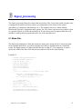
This document describes each module in the library in detail. The applications manual can be
consulted for examples on how to use the modules.
Microb – User’s Manual
3
2
Microb’s General Structure
Microb is made up of a group of modules that allow users to quickly develop robot controllers that
can operate on different platforms. A controller’s level of complexity can vary greatly based on the
type of robot to be controlled and the tasks to be carried out. In the typical case of a serial six DOF
wrist-partitioned robot presented in the applications manual, the use of Microb is greatly simplified
since its inverse kinematic methods already support this type of robot. In addition, in the example
shown, the controller is also one of Microb’s generic controllers.
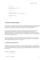
However, in many cases, Microb users will want to provide their own inverse kinematics, develop
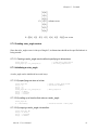
a new controller or spread out the calculations on different platforms. It is therefore important to
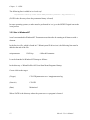
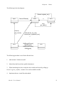
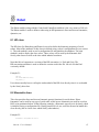
properly understand Microb’s general structure and the tools it contains. These tools are grouped in
nine libraries, which are interrelated, as shown in Figure 1.
con tro lle rs
co ntrol
robo t
re cord
config ura ti on
util ities
vectmath
Figure 1 : Microb’s structure
Microb – User’s Manual
5
Chapter 2 : Microb’s General Structure
2.1 OSDL
The Operating System Dependent Library (OSDL) allows Microb to run under different operating
systems. In fact, this library provides an interface for all functionalities which can vary from one
operating system to another. The following classes are found: Sandglass (clock), Socket (interprocess and inter-CPU communication), Thread (parallel execution threads), Engine (execution
loop), Semaphore (synchronization), and certain functions related to the operating system (random
number generator, task management, etc.). When Microb is migrated to a new operating system,
this is the only library that must be modified. Users are strongly urged to use OSDL classes so that
their code can be reused more easily. To date, OSDL supports SunOS, Solaris 2.6, Linux, QNX,
Irix, VxWorks and WindowsNT.
2.2 Utilities
The Utilities library contains certain utility classes, such as List, which implement linked lists. It
also offers the tools required to develop a client/server type communication. It also contains the
Record class, which allows data to be input for the plotting of graphs.
2.3 Vectmath
The Vectmath library is a set of matrix classes specifically developed for robotics. The following
classes are found: Matrix, Vector, Vector3, Vector4, Vector6, Vector7, Transform, Position,
Angle_axis, Euler_angle, Euler_angle_xyz and Quaternion.
2.4 Signal_processing
The Signal_processing library offers classes that allow data to be filtered. This is particularly useful
when the robot is equipped with sensors with unstable data (e.g. potentiometers, force sensors,
etc.). The available filters are: Mean, Median, Butterworth and Derivative.
2.5 Configuration
The Configuration library contains functions to read and write configuration files. It also allows
configuration subsets to be extracted. The Configuration class is described in Section 8, while the
configuration files used in Microb are presented in Section 1.
6
Microb – User’s Manual
Chapitre 2 : Microb’s General Structure
2.6 Robot
The Robot class (along with the Control and Controllers classes) constitute the very essence of
Microb. This class is used to define a robot using its HD parameters, direct and inverse kinematics,
dynamics, etc.
2.7 Control
The Control module contains the trajectory generation modules and different types of PID
compensators.
Microb – User’s Manual
7
3
OSDL
The Operating System Dependent Library (OSDL) allows Microb to run under different operating
systems. This library provides an interface for all functionalities which can vary from one operating
system to another. The following classes are found: Sandglass (clock), Socket (inter-process and
inter-CPU communication), Thread (parallel execution threads), Engine (peridodic call or
invocation of a function, Semaphore (synchronization), and certain functions related to the
operating system (random number generator, task management, etc.). When Microb is migrated to
a new operating system, this is the only library that must be modified. Users are strongly urged to
use OSDL classes so that their code can be reused more easily. To date, OSDL supports SunOS,
Solaris 2.6, Linux, QNX, Irix, VxWorks and WindowsNT.
3.1 Socket
The Socket class is used to establish fast communication between two threads whether they are
found on the same host or not. The class takes into account the possible difference in the order of
bytes on the different operating systems. Communication can thus be established between a
program running on WindowsNT and another on Solaris. The Socket class allows low-level
communication by socket. The Client and Server classes (see section 4.2) are derived classes which
implement a client/server paradigm with the notion of services.
3.1.1 Socket initialization
Socket communication is done using a server which listens on a specific port on a given host.
Clients can thus transmit and receive data on the host’s port. The Socket class includes both server
and client functions. Only the initialization method is different. With respect to the server, users
can choose to specify the port number or not. It is not recommended that a port number be specified
since it may already be used by another program. With respect to the client, the host name and
server port number must be specified. The server program must thus display on screen the port
number and name of the host being used so that the user can enter them as arguments in the client
process. These operations can be avoided by using a Postmaster. In this respect, the server selects
the port, then registers it with the Postmaster, which then communicates it to the client process. In
such a case, the user need only specify a name to identify the server. Refer to Section 3.2 for
information on how to use a Postmaster.
Exemple 1 : Socket initialization while specifying the port number
// For the server (example on the "amadeus" host)
Microb – User’s Manual
9
Chapter 3 : OSDL
Socket S;
S.init(1715);
...
// For the client
Socket S;
S.init("amadeus", 1715);
// Port number assigned
Exemple 2 : Socket initialization with automatic port assignment
// For the server (example on the "amadeus" host)
Socket S;
S.init();
// Automatic port selection
int port = S.get_port();
...
// For the client
Socket S;
S.init("amadeus", port);
// port is the value returned
// by the server’s S.get_port
Exemple 3 : Socket initialization using the Postmaster
// For the server
Socket S;
S.init("MyServer", "server");
// Automatic port selection and
// recorded with Postmaster as server
...
// For the client
Socket S;
S.init("MyServer", "client");
// The client obtains the name from
// the host and the port number via
// the Postmaster
3.1.2 Socket data transmission
Once the initialization has been completed, the data transfer can be established. The size of the data
transmitted is determined based on the type. The socket class supports the following types of data
transfers: short, int, long, float, double, char *, short *, int *, long *, float *, double *. In the case of
pointers, the number of elements being transmitted or received must be specified. For char pointers,
a character string ending in zero may also be provided. In all cases, the synchronization between
the client and server in terms of the type of data being transmitted must be respected.
Exemple 4 : Transmission between client and server
// Server
#Include "OSDL/socket.h"
short s1 = 2, s2;
double d = 1.4;
static int i5[5] = {1, 2, 3, 4, 5};
char *str = "salut";
Socket S("test", "server");
// Initialization with the Postmaster
S.send(s1);
S.send(d);
S.recv(&s2);
S.send(i5, 5);
S.send(str);
...
10
Microb – User’s Manual
Chapitre 3 : OSDL
// Client
#Include "OSDL/socket.h"
short s1, s2 = 3;
double d;
int i5[5];
char str[20];
Socket S("test", "client");
// Initialization with the Postmaster
S.recv(&s1);
S.recv(&d);
S.send(s2);
S.recv(i5, 5);
S.recv(str);
3.2 Postmaster
The Postmaster is an application that can be used to establish communication between the server
and client on different hosts without the latter knowing where the server actually is. The Postmaster
ensures that communication is established. The use of the Postmaster is not mandatory but it
greatly facilitates the development and use of the client/server applications. To use this type of
connection, the hosts must be correctly registered with the name server (DNS).
The MICPOSTMASTER environment variable must be initialized in the name of the host on which
the Postmaster is running. MICPOSTMASTER uses valid addresses in the following formats:
•
amadeus
•
amadeus.ireq.ca
•
204.19.60.17
3.2.1 Use in Unix
Under Unix, Postmaster is a daemon controlled by inetd. It is not started up manually. inetd opens
the socket to communicate with the clients, launches Postmaster, and establishes a connection
between the client and Postmaster.
To add this service, the user must be in root mode. All of the following operations must be done on
the host where the postmaster is running.
rlogin $MICPOSTMATER
The following line is added in /etc/services:
micpostmaster
12459/tcp
# Microb Postmaster
(12459 can be replaced with any “short” greater than 3400)
Microb – User’s Manual
11
Chapter 3 : OSDL
The following line is added in /etc/inetd.conf:
micpostmaster stream tcp nowait microb PATH/postmaster postmaster /tmp/postmaster.log
(PATH is the directory where the postmaster binary is found)
In some operating systems, a make must be performed in /var/yp or the SIGHUP signal sent to the
inetd process.
3.2.2 Use in WindowsNT
inetd is not standard in WindowsNT. Postmaster must therefore be running at all times as with a
daemon.
In the Services file, which is found in C:\Winnt\system32\drivers\etc\, the following line must be
added at the end of the file:
micpostmaster
12459/tcp
# Microb Postmaster
It can be launched in WindowsNT Startup as follows:
In the directory c:\Winnt\Profiles\All Users\Start Menu\Programs\Startup
Create a link to the target:
(Target:)
C:PATH\postmaster.exe c:\tmp\postmaster.log
(Start in:)
C:PATH
(Run:)
Minimized
Where PATH is the directory where the postmaster.exe program is located.
12
Microb – User’s Manual
Chapitre 3 : OSDL
3.3 Clock (Sandglass)
This class allows users to obtain the time in seconds as accurately as possible. The accuracy varies
based on the OS. Generally, you can expect a maximum error of 10 milliseconds for a non-realtime OS. For a real-time OS, the accuracy rate is less than 1 millisecond. The class methods allow
absolute time to be obtained (Sandglass::absolute()) or relative (Sandglass::delta()). With the
exception of SunOS, you can expect to have good accuracy since Posix-approved functions are
being used.
Exemple 5 :
#include "OSDL/time.h"
Sandglass timer;
double t0 = timer.absolute();
.
.
// Some code
.
double dt = timer.delta();
// Absolute time
// Time since last call of absolute() or delta()
3.4 Semaphore (synchronization)
Data synchronization or protection mechanism between processes or threads. For SunOS, the
semaphores only work between threads. For the other OS, they work between threads and
processes.
In Microb, users may specify, at the time the semaphore is being created or initialized, whether it is
to be made available. By default, the semaphores are not available when being created; users must
perform a give() to make them available.
Exemple 6 : ex_semaphore.C
#include "OSDL/semaphore.h"
#include "OSDL/thread.h"
Semaphore sem;
int entiers[30];
/*
Place the 4 lines which begin with sem as comments. For the 2nd test,
if the Semaphore is removed, the program output is no longer the same each time
each time it is run. Main does not wait for thread to be finished writing to fill in the
vector -> at the end, the vector will consist of a undefined combination of 1 and 0.
*/
void function1(void *)
{
sem.take();
printf("function1 : I have the semaphore\n");
for(int j=0;j<30;j++) entiers[j] = 1;
mc_thread_sleep(5.0);
printf("function1 : I give back the semaphore\n");
sem.give();
Microb – User’s Manual
13
Chapter 3 : OSDL
}
int main(int, char**)
{
int i;
Thread th(function1, 0, 8192, "Function1", 0.5);
printf("main : I give the semaphore\n");
sem.give();
sem.take();
printf("main : I have taken back the semaphore\n");
for(i=0;i<30;i++) integers[i] = 0;
printf("main : The vector is:\n");
for(i=0;i<30;i++) printf("%d \n",integers[i]);
return 0;
}
To make the semaphore available from the start, the following must be added:
sem.init(Semaphore::Full);
and sem.give() must be removed in main().
3.5 Thread
The Thread class has a function parallelization mechanism. It allows a task to start up other tasks in
parallel without having to stop the program. The threads of a process share the same resources (e.g.
memory).
Exemple 7 : ex_threads.C
/****************************************************************************
* MICROB (Modules Intégrés pour le Contrôle de ROBots)
* Copyright (C) 1996-2002 Hydro-Québec
* Institut de recherche d'Hydro-Québec (IREQ)
* 1800, boul. Lionel-Boulet, Varennes (Québec) Canada J3X 1S1
* [email protected], http://www.robotique.ireq.ca
*
* This library is free software; you can redistribute it and/or
* modify it under the terms of the GNU Lesser General Public
* License as published by the Free Software Foundation; either
* version 2.1 of the License, or (at your option) any later version.
*
* This library is distributed in the hope that it will be useful,
* but WITHOUT ANY WARRANTY; without even the implied warranty of
* MERCHANTABILITY or FITNESS FOR A PARTICULAR PURPOSE. See the GNU
* Lesser General Public License for more details.
*
* You should have received a copy of the GNU Lesser General Public
* License along with this library; if not, write to the Free Software
* Foundation, Inc., 59 Temple Place, Suite 330, Boston, MA 02111-1307 USA
***************************************************************************/
#include <stdio.h>
#include "OSDL/thread.h"
void function1(void *)
{
printf("function1 : start\n");
mc_thread_sleep(2);
printf("function1 : end\n");
}
14
Microb – User’s Manual
Chapitre 3 : OSDL
void function2(void *)
{
printf("function2 : start\n");
mc_thread_sleep(1);
printf("function2 : end\n");
}
int main(int, char**)
{
printf("main : start\n");
Thread fils1(function1, 0, 8192, "Function1", .5);
Thread fils2(function2, 0, 8192, "Function2", .5);
mc_thread_sleep(4);
printf("main : end\n");
return 0;
}
3.6 Periodic function (Engine)
This module is used to append a function that will be called up periodically at a frequency specified
by the user. On a real-time OS, the period will be guaranteed. For other operating systems, the
period will be met insofar as possible. This class is the core of Microb controllers.
The Engine class allows to have several real-time loops running at different frequencies. The
Engine module is built such that each instance of the class is entered in a static table. The
initialization method of each real-time loop may then establish the basic period shared by all the
registered loops and make it its main period. Then, at each iteration of the main loop, the functions
of each loop are called up in turn.
One of the disadvantages of this is the delay caused by the time required to execute the function.
Thus, if three functions are registered and the execution time of the first two is not constant, the
period of the third method will not be very consistent.
3.6.1 Starting up a periodic loop
A periodic loop is started up in two stages: initializing (using the constructor or init method) and
the actual startup (using the start method). A loop can be stopped using the stop method and started
up again as desired. In the following example, my_function will be called up at a frequency of 50
Hz (1/.02 sec).
Exemple 8 : Using an Engine
#include "OSDL/engine.h"
Microb – User’s Manual
15
Chapter 3 : OSDL
Engine engine;
double period = .02;
double priority = .5;
void *arg = (void*)&engine;
// In seconds
// Between 0 and 1
engine.init(REAL, period, my_function, arg, priority);
engine.start();
mc_thread_sleep(5);
// Allowed to run for 5 seconds
engine.stop();
// Engine is stopped
The function that is called up will have the following syntax:
void my_function(void *ptr)
{
}
where the pointer ptr is the 4th argument passed to the Engine::init method. In the example above,
it is the Engine object’s address.
3.6.2 Detecting non-periodicity
During robot control, control loop periodicity is often crucial. The Engine class uses two methods
to check whether the periodicity is met at each iteration. First, Engine checks that the function
called up is of a duration less than the period requested. Then, Engine ensures that the last period
has not been overly long thanks to the following algorithm:
if(last_period*tolerance > desired_period)
{
// The warning function is called
...
}
The last_period variable represents the time elapsed from the start of the periodic function during
the previous iteration to the start of this function during the current iteration. This period may differ
from the desired period if the time required to execute the periodic function is greater than the
desired period and/or if another task has higher priority on the system than the control loop. The
value of the tolerance variable must be found between 0 and 1, where 1 represents perfect
periodicity. The Engine::get_tolerance() and Engine::set_tolerance() methods are used to read and
modify this value. The acceptable tolerance level will obviously depend on the application. In
addition, on a non-real-time system, most of the time this value will have to be decreased. For
instance, the Solaris operating system will not allow any interruption between two instructions in a
task to continue executing the control loop. This method thus does not ensure periodicity. However,
it minimizes the risk of data becoming corrupted. These systems are of course not recommended
for robot force and velocity control.
If non-periodicity is detected, the mc_overrun_warning() function is called up by default. This
function prints out, in the following sequence, a warning message, the desired period, the duration
of the last period, and the time required by the CPU to execute the periodic function. If this time
exceeds the desired period, the latter value has to be increased. However, if the last period is greater
16
Microb – User’s Manual
Chapitre 3 : OSDL
than the desired period, the user must decrease the tolerance and/or increase the number of clock
overrun permits (nb_overrun_max attribute in the Engine class). The
Engine::set_overrun_function() method is used to specify that another function is to be called up if
non-periodicity is detected. This is especially useful when the robot needs to be stopped
immediately.
3.6.3 Recording synchronous data
The Engine class is used to record data synchronously (i.e. at each iteration). The record method is
used to specify an input function, a data pointer and the size of the table that is to be recorded. Data
recording begins when this method is called or, if the engine is not running, when the start method
is called. The get_record method is used to obtain the table where the data are entered while the
save_record method is used to save the data in a file.
The following example illustrates the use of this function. An engine is created that calls up a
periodic function. This function displays the time elapsed between two iterations. The record
method is used to record three data during eight iterations. The three data are the time elapsed since
the last iteration, a counter, and the period requested. This last parameter is a pointer passed as an
argument to the record method. A pointer to the controller’s class is normally used to access
relevant data.
Exemple 9 : Inputing data
#include "OSDL/osdl.h"
#include <stdio.h>
static void periodic_func(void *)
{
static Sandglass my_clock;
static int cpt = 0;
printf("%3d – This message must be displayed periodically (period = %g)\n",
cpt++, my_clock.delta());
}
void rec_func(void *p_arg, double *p_record)
{
static Sandglass my_clock;
static int i = 0;
p_record[0] = my_clock.delta();
p_record[1] = i++;
p_record[2] = *((double *)p_arg);
}
void main(void)
{
Engine engine;
const double per = .5;
// seconds
const double laps = 5.0; // seconds
Sandglass my_clock;
int nb_data = 3, nb_iter = 8;
engine.init(AUXILIARY, per, periodic_func, 0, 0.5);
engine.record(rec_func, (void*)&per, nb_data, nb_iter);
engine.start();
Microb – User’s Manual
17
Chapter 3 : OSDL
// Engine left to run for 5 seconds
double t0 = my_clock.absolute();
while(my_clock.absolute() - t0 < laps)
{
mc_thread_yield();
}
// Engine is stopped
engine.stop();
// Data on screen are printed out
double **p_record = engine.get_record();
printf("Test for record\n");
for(int i = 0; i < nb_iter; ++i)
{
for(int j = 0; j < nb_data; ++j)
{
printf("%g ", p_record[i][j]);
}
printf("\n");
}
//Data are recorded in a file
engine.save_record("foo.xyz");
}
3.7 Random number generator
The functions mc_seed and mc_random provide a standard interface for the generation of random
numbers regardless of the type of operating system used. In the following example, 10 numbers are
generated between -0.5 and 0.5.
Example 10: Random number generator
#include "OSDL/random.h"
double d;
mc_seed();
for(int i = 0; i < 10 ; ++i)
{
d = mc_random(-0.5, 0.5);
printf("d = %g\n", d);
}
3.8 Shared memory (Shmem)
The Shmem class has a mechanism for sharing data between processes running on the same host
through a shared memory area. The class is initialized using a key and the size of the memory area
that is to be allocated. The Shmem::addr() method is used to obtain a pointer for the allocated
memory address. If the allocation fails, the pointer will be nil.
Example 11: Data sharing used a shared memory
// Process 1
18
Microb – User’s Manual
Chapitre 3 : OSDL
Shmem data(1234, 10*sizeof(double));
double *d = (double*)data.addr();
for(int i = 0; i < 10; i++)
d[i] = i*2.5;
...
// Process 2
Shmem data(1234, 10*sizeof(double));
double *d = (double*)data.addr();
for(int i = 0; i < 10; i++)
printf("d[%d] = %g \n", i, d[i]);
Note that the size of the allocated memory is taken into account only at the first initialization. This
allows a process to allocate a variable amount of memory and to send this size information to
another shared-memory process. Note also that the class’ destructor does not free up the memory.
The Shmem::free() method must be called up specifically by one of the processes.
Microb – User’s Manual
19
4
Utilities
This library contains certain utility classes such as List which implement the chained lists.
4.1 List
The List class allows the user to create and manipulate a list of pointers. Different methods are used
to add (insert), remove (remove) or retrieve (get_ptr) elements. It is also possible to print (print) the
list or delete it (delete_all).
Example 12:
#include "Utilities/list.h"
List list;
double item1 = 1.2, item2 = 3.4, *item;
// Add 2 elements in the list
list.insert("First item", (void*)&item1);
list.insert("Second item", (void*)&item2);
// Print out the list
list.print();
// Get an item
item = (double*) list.get_ptr("Second item");
printf("Item = %g\n", *item);
// Remove an item
list.remove("First item");
// Print out the list again
list.print();
// Delete the list (optional in this example
// since the List destructor calls up this method)
liste.delete_all();
4.2 Client and Server
The Server class is derived from the Socket class. It allows the user to quickly implement a server
capable of handling several requests. When the class is initialized, the user enters a name for the
server. When initializing a Client-type object, the server’s name is entered (if a Postmaster is being
Microb – User’s Manual
21
Chapter 4 : Utilities
used) or a host name and port. The server provides ServerFcn-type functions. The Server class
offers the following default services: StartRecordDemand, PrintRecordedDemand,
DeleteRecordedDemand and StopRecordDemand. These services allow the user to begin recording
service requests, printing them out, deleting the list, or stopping the input process.
Example 13:
// Services
Matrix fonction1(Server &, Message)
{
printf("Service 1 was called\n");
}
Matrix fonction2(Server &, Message)
{
printf("Service 2 was called\n");
}
// Server
main()
{
Server simple_server("Simple_server");
simple_server.register_service("Service1", fonction1);
simple_server.register_service("Service2", fonction2);
simple_server.loop();
}
.
.
.
// Client
main()
{
// Connected to server
Client my_client("Simple_server");
// Request list of services available from server
client.get_service();
// Print out list of available services
printf("Service disponible : \n");
client.service.print(0);
// Call up services
client.execute("Service1", "");
client.execute("Service2", "");
// Ask server to end
client.close_server();
}
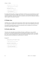
4.3 Record
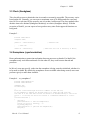
This class allows the user to record the data from variables over a desired period of time. By using
tools such as Gnuplot or Excel, users can plot graphs and analyze the data recorded.
22
Microb – User’s Manual
Chapitre 4 : Utilities
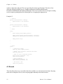
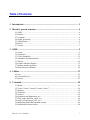
The following is the class diagram:
Record::register_var()
Engine
1:1
Record
Record::refresh()
1:N
Device
rec()
get_name()
record()
get_record()
1:1
Record::set_rec_var()
Record::get_registered_var()
1:1
Server
SetRecordChoice()
StartRecord()
Client
GetRecordChoice()
GetRecord()
1:N
The following procedure is used for the Record class:
1.
Add #include “Utilities/record.h”
2.
Inherit from the Record class (public inheritance).
3. When initializing the class, record the class variables in Record by calling up
Record::register_var(this, “varname”) for each recordable variable.
4.
Implement the two virtual Record methods.
Microb – User’s Manual
23
Chapter 4 : Utilities
double rec(const char*name): this method is used to compare the variable name passed as a
parameter with the names of the recordable class variables and return the value of the variable if it
exists. When the variable being sought does not exist, the value of -1 must be returned.
const char*get_name(void) const: this method is used to return a unique name for the class or
peripheral.
5.
Implement the access methods in the client and server class (see the class diagram above).
In Microb, the Device class already inherits from the Record class.
Refer to the Utilities/Tests/test_record.C file for an example of how the Record class is used.
24
Microb – User’s Manual
5
Vectmath
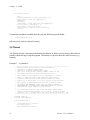
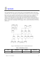
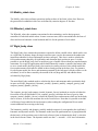
The Vectmath module has a series of classes used to create and manipulate matrices and vectors.
The Matrix class covers the general case of MxN matrices, while the Vector class is used to handle
Mx1 or 1xN vectors. It inherits from the Matrix class. The other classes have set dimensions and
inherit from either a Matrix or Vector. They express, for the most part, a pure orientation
(Angle_axis, Rotation, Quaternion, Euler_angle), pure position (Position) or both (Transform,
Angle_axis_xyz, Quaternion_xyz et Euler_angle_xyz). Vector3, Vector4, Vector6 and Vector7 are
generic classes for given vectors with dimensions of 3, 4, 6 or 7. They have no specific properties.
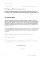
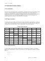
Figure 1 : shows these relationships in UML language. Table 1 shows the dimensions of each class
and their use.
Figure 1: Relationship between the Vectmath module classes
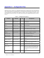
Table 1: Information on classes
Class
Matrix
Dimension
MxN
Microb – User’s Manual
Expresses
General matrix
Inherits from
–
25
Chapter 5 : Vectmath
Vector
M x 1 or 1 x N
General vector
Matrix
Vector3
3 x 1 or 1 x 3
Vector of length 3
Vector
Vector4
4 x 1 or 1 x 4
Vector of length 4
Vector
Vector6
6 x 1 or 1 x 6
Vector of length 6
Vector
Vector7
7 x 1 or 1 x 7
Vector of length 7
Vector
Transform
4x4
Orientation and position
Matrix
Rotation
3x3
Orientation
Matrix
Position
3 x 1 or 1 x 3
Position
Vector3
Quaternion
4 x 1 or 1 x 4
Orientation
Vector4
Euler_angle
3 x 1 or 1 x 3
Orientation
Vector3
Angle_axis
3 x 1, 1 x 3, 4 x 1 or 1 x 4
Orientation
Vector
Quaternion_xyz
7 x 1 or 1 x 7
Orientation and position
Vector7
Euler_angle_xyz
6 x 1 or 1 x 6
Orientation and position
Vector6
Angle_axis_xyz
6 x 1, 1 x 6, 7 x 1 or 1 x 7
Orientation and position
Vector
The following sections describe each of these classes. The Vector, Vector3, Vector4, Vector6 and
Vector7 classes are described in the same chapter given their considerable similarities. The same
applies for classes with the extension _xyz, which are described in the same section as classes
without extensions.
5.1 Matrix
5.1.1 Introduction
The Matrix class is used to perform basic matrix calculations such as multiplication, addition,
division, inversion, etc. The matrices can be of any given dimension. Since the Matrix class
methods are general in nature, they are not optimized for special cases such as homogenous 4x4
matrices, vectors, quarternions, etc.
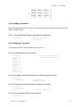
An A(nrow, ncol) matrix will have nrow lines and ncol columns. The referencing of the element
found on the 3rd line and in the 2nd column of matrix A is notated A[2][1] since the lines and
columns are numbered starting from 0:
26
Microb – User’s Manual
Chapitre 5 : Vectmath
A[0][0]
A[0][1]


A[1][0]
A[1][1]
A=

...
...

 A[nrow − 1][0] A[nrow − 1][1]
...
A[0][ncol − 1] 
...
A[1][ncol − 1] 

...
...

... A[nrow − 1][ncol − 1]
5.1.2 Creating matrices
There are two ways to create a matrix:
5.1.2.1 Without specifying the dimensions
Matrix A;
// Dimensions should be defined later
5.1.2.2 By specifying the dimensions
Matrix B(2, 3)
// Create a 2x3 matrix
5.1.3 Initializing a matrix
A matrix can be initialized in several ways:
5.1.3.1 By specifying one term at a time
Matrix A(2, 3);
A[0][0] = 1;
A[0][1] = 2;
A[0][2] = 3;
A[1][0] = 4;
A[1][1] = 5;
A[1][2] = 6;
// Create a 2x3 matrix
// Initialize the element 0, 0
5.1.3.2 By calling up a function that returns a matrix
Matrix A;
A = mc_identity(2);
Position p(1, 2, 3);
A = mc_diag(p);
A = mc_jordan(5, 6);
// A will be a 2x2 matrix
// A will be a 3x3 diagonal matrix
// A will be a 5x5 Jordan matrix
// with 6s on the diagonal
5.1.3.3 By copying one matrix into another
Matrix A, B;
A = mc_identity(3);
B = A;
// A will be copied into B
5.1.3.4 By copying the result of an operation,
Matrix A, B(2, 2), C;
A = mc_identity(2);
Microb – User’s Manual
27
Chapter 5 : Vectmath
B[0][0] =
B[0][1] =
B[1][0] =
B[1][1] =
C = A*B;
1;
2;
3;
4;
// The product of A*B will be put in C
5.1.4 Matrix functions
5.1.4.1 Addition
A
A
A
A
A
= B + C;
= B + s;
= s + B;
+= B;
+= s;
// Of 2 matrices
// Of a matrix and a scalar
// Of a scalar and a matrix
5.1.4.2 Subtraction
A
A
A
A
A
= B - C;
= B - s;
= s - B;
-= B;
-= s;
// Of 2 matrices
// Of a matrix and a scalar
// Of a scalar and a matrix
5.1.4.3 Multiplication
A
A
A
A
A
= B*C;
= B*s;
= s*B;
*= B;
*= s;
// Of 2 matrices
// Of a matrix and a scalar
// Of a scalar and a matrix
5.1.4.4 Division
A
A
A
A
A
= B/C;
= B/s;
= s/B;
/= B;
/= s;
// Of 2 matrices -> inv(C)*B
// Of a matrix and a scalar
// Of a scalar and a matrix
5.1.4.5 Inversion
A = mc_inv(B);
A = 1/B;
5.1.4.6 Transposition
A = mc_transpose(B);
5.1.5 Analyzing a matrix
5.1.5.1 Dimensions
number_of_columns = A.ncol();
number_of_rows = A.nrow();
28
Microb – User’s Manual
Chapitre 5 : Vectmath
5.1.5.2 Determinant
d = mc_det(A)
5.1.5.3 Eigenvalues
mc_eigen_values(A, (double_complex *)vp);
// Find eigenvalues
if(mc_eigen_values(A) == 1)
// Check whether eigenvalues are positive
5.1.5.4 Trace
t = mc_trace(A);
5.1.5.5 Minimum and maximum values
min = A.min();
max = A.max();
5.1.6 Binary tests
5.1.6.1 Equality
if(A == B)
if(A == s)
// If A is 1x1 and a value of s
5.1.6.2 Difference
if(A != B)
if(A != s)
// If A is not 1x1 or a value of s
5.1.7 Creating submatrices
5.1.7.1 Deleting a column
A = mc_del_col(B, col);
// Delete column col
5.1.7.2 Deleting a row
A = mc_del_row(B, row);
// Delete row
5.1.7.3 Deleting a row and a column
A = mc_sub_matrix(B, row, col);
// Delete column col
// and row
5.1.7.4 Extracting a region
// Only keep submatrix which extends from column x1
// to column x2 and from row y1 to row y2
A = mc_sub_matrix(B, y1, x1, y2, x2);
Microb – User’s Manual
29
Chapter 5 : Vectmath
5.1.7.5 Extracting a column
(Vector) V = A.col(x);
// Extracting column x
5.1.7.6 Extracting a line
(Vector) V = A.row(y);
// Extracting row y
5.1.7.7 Absolute-value matrix
B = mc_abs(A);
5.1.7.8 Modifying matrices
5.1.7.9 Swapping columns
A.swap_col(x1, x2);
5.1.7.10 Swapping rows
A.swap_row(y1, y2);
5.1.8 Matrix file operations
5.1.8.1 Save
A.save("MyMatrix.mat");
// Saved in MyMatrix.mat
5.1.8.2 Read
A.load("MyMatrix.mat");
// Read in MyMatrix.mat
5.2 Vector, Vector3, Vector4, Vector6, Vector7
5.2.1 Introduction
Vector, Vector3, Vector4, Vector6 and Vector7 are classes derived from the Matrix class. They
support special vector cases. All of the Matrix functions are available if applicable. In addition,
some of them may have been optimized in order to take advantage of the vector’s specialization.
The Vectors may be of any length, whereas VectorX is of lengh X.
There are two types of vectors: column vectors and row vectors. Column vectors are a special case
of a (nrow x 1) matrix, and row vectors are a special case of a (1 x ncol) matrix. The referencing of
the nth element of a row vector or column V vector is notated V[x - 1] since indexing starts at 0:
30
Microb – User’s Manual
Chapitre 5 : Vectmath
5.2.2 Creating vectors
There are two ways to create a vector:
5.2.2.1 Without specifying the dimensions
Vector V;
Vector3
Vector4
Vector6
Vector7
V1;
V2;
V3;
V4;
//
//
//
//
//
//
Row or column vector:
dimensions will have to
Column vector of length
Column vector of length
Column vector of length
Column vector of length
be defined
3
4
6
7
5.2.2.2 By specifying the dimensions
Vector V1(3);
// Column vector of length 3
Vector V(4);
// Column vector of length 4
Vector V2 = mc_transpose(4);
// Row vector of length 4
Vector3 = mc_transpose(3);
// Row vector of length 3
Vector4 = mc_transpose(4);
// Row vector of length 4
// NOTE: Vector3 V(x); Will create a vector of length 3
// NOTE: using all the elements initialized at x
// NOTE: Vector4 V(x); Will create a vector of length 4
// NOTE: using all the elements initialized at x
// NOTE: Vector6 V(x); Will create a vector of length 6
// NOTE: using all the elements initialized at x
// NOTE: Vector6 V(x); Will create a vector of length 6
// NOTE: using all the elements initialized at x
5.2.3 Initializing a vector
A vector can be initialized in several ways:
5.2.3.1 By specifying one term at a time
Vector V1(3);
V1[0] = 1;
V1[1] = 2;
V1[2] = 3;
Vector V2 = mc_transpose(2);
V2[0] = 4;
V2[1] = 5;
// Create a vector of length 3
// Initialize element 0
// Vector of length 2
5.2.3.2 By calling up a function that returns a vector
Vector V;
Matrix A = mc_identity(3)*2.5;
V = mc_diag(A);
// mc_diag(A) returns the diagonal of A
5.2.3.3 By copying one vector into another
Vector V1(2), V2;
V1[0] = 1;
V1[1] = 2;
V2 = V1;
Microb – User’s Manual
// V1 will be copied into V2
31
Chapter 5 : Vectmath
5.2.3.4 By copying the result of an operation
Vector V1(2), V2;
double d = 3.0;
V1[0] = 1;
V1[1] = 2;
V2 = V1*d;
// The product of V1*d will be inserted in V2
5.2.3.5 Using the constructor (available for VectorX only)
Vector3
Vector4
Vector3
Vector4
V1(1.2, -.34, 45);
V2(1.2, -.34, 45, .03);
V3(1.5);
V4(1.5);
// All the elements will be 1.5
// All the elements will be 1.5
5.2.4 Vectorial functions
5.2.4.1 Inversion
V1 = mc_pinv(V2);
V1 = 1/V2;
5.2.4.2 Transposition
V1 = mc_transpose(V2);
5.2.4.3 Extracting an element
(double) V = A.get(x);
// Extract element x
5.2.4.4 Scalar product and vectorial product
(double) d = mc_scalar_product(A, B);
C = mc_vectorial_product(A, B);
5.3 Rotation
5.3.1 Introduction
The Rotation class is used to perform matrix calculations on rotation matrices. The rotation matrics
are orthonormal 3x3 matrices. All of the Matrix functions are available. In addition, some of them
may have been optimized to take advantage of the specialization of the rotation matrix. For
instance, a rotation matrix will have a much faster inversion than a regular matrix will.
A matrix with a rotation R will have three rows and three columns. The referencing of the element
located on the 3rd row and in the 2nd column will be notated R[2][1] since the rows and columns
are numbered starting from 0:
32
Microb – User’s Manual
Chapitre 5 : Vectmath
 R[0][0] R[0][1] R[0][2]
R =  R[1][0] R[1][1] R[1][2] 
 R[2][0] R[2][1] R[2][2]
5.3.2 Creating a rotation matrix
Since the rotation matrix is always 3x3, the dimensions are not specified when the matrix is being
created.
5.3.3 Creating a matrix without specifying the dimensions
Rotation A;
// Dimensions do not need to be
// defined
5.3.4 Initializing a rotation matrix
A rotation matrix can be initialized in several ways:
5.3.4.1 By specifying one term at a time
Rotation A;
A[0][0] = 0;
A[0][1] = 1;
A[0][2] = 0;
A[1][0] = 1;
A[1][1] = 0;
A[1][2] = 0;
A[2][0] = 0;
A[2][1] = 0;
A[2][2] = 1;
// Create a rotation matrix
// Initialize the element 0, 0
5.3.4.2 By calling up a function that returns a rotation matrix
Rotation A;
A = mc_identity(3);
// The 3x3 matrix is
// a rotation matrix
5.3.5 Matrix functions
5.3.5.1 Eigenvalues
// Find the eigenvalues
mc_eigen_values(A, (double_complex *)vp);
// Check whether the eigenvalues are positive
if(mc_eigen_values(A) == 1)
Microb – User’s Manual
33
Chapter 5 : Vectmath
5.3.5.2 Vect
Vector v = mc_vect(R);
// Return the vect of matrix R
5.3.6 Modifying a rotation matrix
5.3.6.1 Orthonormalization
There are three orthonormalization methods. The first one that gives the best theoretical solution
uses singular value decomposition: R = U*S*transpose(V), Rortho = U*transpose(V), where U and
V are orthogonal and S is diagonal. The other two methods are much faster but give a slightly
different solution than the best theoretical solution. The ortho_very_fast method gives excellent
results for most applications.
// Orthonormalizes R using singular value decomposition
R.ortho();
// Orthonormalizes R using the vectorial product
R.ortho_fast();
// Orthonormalizes R by converting it to an Angle_axis then back to a Transform
R.ortho_very_fast();
5.4 Transform
5.4.1 Introduction
The Transform class is used to perform matrix calculations on 4x4 homogenous matrices. All of the
Matrix functions are available. In addition, some of them may have been optimized to take
advantage of the specialization of the homogenous matrix. For instance, a homogenous matrix
inversion will be much faster than that of an ordinary matrix.
A homogenous matrix T will have 4 rows and 4 columns. The referencing of the element found on
the 3rd row and in the 2nd column of homogenous matrix R will be notated R[2][1] since the rows
and columns are numbered starting from 0:
T [0][0]
 T [1][0]
T =
T [2][0]

T [3][0]
T [0][1]
T [1][1]
T [2][1]
T [3][1]
T [0][2]
T [1][2]
T [2][2]
T [3][2]
T [0][3]
T [1][3] 
T [2][3]

T [3][3]
Note that a homogenous matrix is in fact made up a rotation matrix and a position vector (x, y, z):
34
Microb – User’s Manual
Chapitre 5 : Vectmath
 R[0][0] R[0][1] R[0][2]
 R[1][0] R[1][1] R[1][2]
T =
 R[2][0] R[2][1] R[2][2]

0
0
 0
x
y 
z

1
5.4.2 Creating a Transform
Since the homogenous matrix is always 4x4, the dimensions should not be specified when the
matrix is being created:
5.4.2.1 Creating the matrix without specifying the dimensions
Transform A;
// Dimensions do not need
// to be defined
5.4.3 Initializing a Transform
A homogenous matrix can be initialized in several ways:
5.4.3.1 By specifying one term at a time
Transform
A[0][0] =
A[0][1] =
A[0][2] =
A[1][0] =
A[1][1] =
A[1][2] =
A[2][0] =
A[2][1] =
A[2][2] =
A;
0;
1;
0;
1;
0;
0;
0;
0;
1;
// Creating a homogenous matrix
// Initializing the element 0, 0
A[0][3] = 2.0;
A[1][3] = 3.4;
A[2][3] = -1.4;
5.4.3.2 By calling up a function that returns a 4x4 homogenous matrix
Transform A;
A = mc_identity(4);
// The 4x4 matrix is
// a homogenous matrix
5.4.3.3 By copying one 4x4 homogenous matrix into another
Transform A, B;
A = mc_identity(4);
B = A;
// A will be copied into B
5.4.3.4 By copying the product of an operation
Transform A, B, C;
Microb – User’s Manual
35
Chapter 5 : Vectmath
A = mc_identity(4);
B[0][0] = 1;
B[0][1] = 0;
B[0][2] = 0;
B[1][0] = 0;
B[1][1] = 0;
B[1][2] = 1;
B[2][0] = 0;
B[2][1] = 1;
B[2][2] = 0;
B[0][3] = 2.0;
B[1][3] = 3.4;
B[2][3] = -1.4;
C = A*B;
// The product of A*B will be inserted into C
5.4.4 Matrix functions
5.4.4.1 Transposition
// NOTE: The rotation part is transposed while
// NOTE: the position part is lost
A = mc_transpose(B);
5.4.5 Modifying the Transform
5.4.5.1 Orthonormalization
Orthonormalization applies to the rotation part of the Transform. See the note in section 5.3.6.1.
// Orthonormalizes T using the singular value décomposition
T.ortho();
// Orthonormalizes T using the vectorial product
T.ortho_fast();
// Orthonormalizes T by converting it to an Angle_axis then back to a Transform
T.ortho_very_fast();
5.5 Position
5.5.1 Introduction
The Position class is derived from the Vector class. It supports special vector-position cases. All of
the Vector functions are available if applicable. In addition, some of them may have been
optimized to take advantage of the position-vector specialization. Position-vectors have a length of
3 and form of (x, y, z). They can still be used as homogenous vectors of form (x, y, z, 1).
There are two types of position-vectors: column position-vectors and row position-vectors. The
referencing of the nth element in a given row or column P is notated P[x - 1] since indexing begins
at 0:
36
Microb – User’s Manual
Chapitre 5 : Vectmath
 x
P =  y  : column position-vector
 z 
P = [x
y
z ] : row position-vector
5.5.2 Creating position-vectors
Since a position-vector always has a length of 3, its dimensions do not need to be specified when it
is being created:
5.5.2.1 Creating a position-vector without specifying the dimensions
Position P1;
Position P2 = mc_transpose(3);
// Column position vector
// Row position vector
5.5.3 Initializing a position
A position can be initialized in several ways:
5.5.3.1 By specifying one term at a time
Position V(.5, .3, 1);
Position V1;
V1[0] = 1;
V1[1] = 2;
V1[2] = 3;
Position V2 = mc_transpose(3);
V2[0] = 4;
V2[1] = 5;
V2[2] = 6;
// When being created
// Create a column position
// Initialize element 0
// Row position
5.5.3.2 By calling up a function that returns a position
Position P;
P = functionx();
// functionx returns a position
5.5.3.3 By copying a position into another position
Position V1, V2;
V1[0] = 1;
V1[1] = 2;
V1[2] = 3;
V2 = V1;
// V1 will be copied into V2
5.5.3.4 By copying the result of an operation
Position V1, V2;
double d = 3.0;
Microb – User’s Manual
37
Chapter 5 : Vectmath
V1[0] = 1;
V1[1] = 2;
V1[2] = 3;
V2 = V1*d;
// The product of V1*d will be inserted into V2
5.5.3.5 Using the constructor
Position V1(1.2, -.34, 45);
Position V2(1.5);
// All the elements will be 1.5
5.5.4 Vector functions
5.6 Quaternion and Quaternion_xyz
5.6.1 Introduction
The Quaternion class is derived from the Vector class. It supports special quaternion-vector cases.
All of the Vector functions are available if applicable. In addition, some of them may have been
optimized to take advantage of the quaternion-vector specialization. Quaternion-vectors have a
length of 4 and form of (q0, q1, q2, q3).
There are two types of quaternion-vectors: column quaternion-vectors and row quaternion-vectors.
The referencing of the nth element in a given quaternion row or column Q will be notated Q[x - 1]
since indexing begins at 0:
Q[0]
 Q[1] 
 : column quaternion-vector
Q=
Q[2]


Q[3]
Q = [Q[0] Q[1] Q[2] Q[3]]: row quarternion-vector
Unit quaternions
The unit quaternion is a special case. It is also known as “Euler’s parameters” or “Euler’s
Quaternion” and is especially useful for expressing rotation in space. Most of the library
constructors return a unit quaternion with the exception of the direct initialization of the vector
elements. Following algebraic (addition, subtraction, etc.) or other types of calculations, it is up to
the user to render the unit quarternion when needed (see the unit method).
38
Microb – User’s Manual
Chapitre 5 : Vectmath
5.6.2 Creating quaternion-vectors
Since the quaternion-vector is always of length 4, its dimensions should not be specified when it is
being created:
5.6.2.1 Creating a quaternion-vector without specifying its dimensions
Quaternion Q1;
Quaternion Q2 = mc_transpose(4);
// Column quaternion vector
// Row quaternion vector
5.6.3 Initializing a quaternion
A quaternion can be initialized in several ways:
5.6.3.1 By specifying one term at a time
Quaternion Q1;
Q1[0] = 1;
Q1[1] = 0;
Q1[2] = 0;
Q1[3] = 0;
Quaternion Q2 = transpose(4);
Q2[0] = 0.68825;
Q2[1] = -0.555325;
Q2[2] = -0.21525;
Q2[3] = 0.414239;
// Create a column quaternion
// Initialize the element 0
// Row quaternion
5.6.3.2 By calling up a function that returns a quaternion
Quaternion Q;
Q = functionx();
// functionx returns a quaternion
5.6.3.3 By copying a quaternion into another
Quaternion Q1, Q2;
Q1[0] = 0.741713;
Q1[1] = -0.130604;
Q1[2] = 0.594085;
Q1[3] = 0.282607;
Q2 = Q1;
// Q1 will be copied into Q2
5.6.3.4 By copying the result of an operation
Quaternion Q1, Q2, Q3;
Q1[0] = 0.741713;
Q1[1] = -0.130604;
Q1[2] = 0.594085;
Q1[3] = 0.282607;
Q2 = Q1;
Q3 = Q1*Q2;
Microb – User’s Manual
// The product of Q1*Q2 will be inserted into
// Q3
39
Chapter 5 : Vectmath
5.6.4 Vector functions
5.6.4.1 Square
V1 = mc_square(v2);
5.6.5 Analyzing a quaternion
5.6.5.1 Norm
double d = Q.norm();
5.6.5.2 Absolute value
double d = Q.abs();
5.7 Euler_angle and Euler_angle_xyz
5.7.1 Introduction
The Euler_angle class is derived from the Vector class. It supports specific Euler angle cases. All of
the Vector functions are available if applicable. In addition, some of them may have been
optimized to take advantage of the Euler angle specialization. Euler_angles have a length of 3 and
form of (roll, pitch, yaw).
There are two types of euler_angle-vectors: column euler_angle-vectors and row euler_anglevectors. The referencing of the nth element of a euler_angle row or column E is notated E[x - 1]
since indexing begins at 0:
 E[0]
E =  E[1]  : column vector
 E[2]
E = [E[0] E[1] E[2]]: row vector
The Euler_angle_xyz class is equivalent to the Euler_angle class but also contains a Position
vector:
40
Microb – User’s Manual
Chapitre 5 : Vectmath
 E[0]
 E[1] 


 E[2]


E =  E[3] : column vector
 E[4]


 E[5]
 E[6]


E = [E[0] E[1] E[2] E[3] E[4] E[5] E[6]] : row vector
5.7.2 Creating euler_angle-vectors
Since the euler_angle-vector is always of length 3, its dimensions should not be specified when it is
being created:
5.7.2.1 Creating a euler_angle-vector without specifying its dimensions
Euler_angle Q1;
Euler_angle Q2 = mc_transpose(3);
// Column euler_angle-vector
// Row euler_angle-vector
5.7.3 Initializing a euler_angle
A euler_angle can be initialized in several ways:
5.7.3.1 By specifying one term at a time
Euler_angle E1;
E1[0] = 1;
E1[1] = 0;
E1[2] = 0;
Euler_angle E2 = mc_transpose(3);
E2[0] = 0.68825;
E2[1] = -0.555325;
E2[2] = -0.21525;
// Create a euler_angle-column
// Initialize element 0
// Euler_angle-row
5.7.3.2 By calling up a function that returns a euler_angle
Euler_angle E;
E = functionx();
// functionx returns a euler_angle
5.7.3.3 By copying a euler_angle into another
Euler_angle E1, E2;
E1[0] = 0.741713;
E1[1] = -0.130604;
E1[2] = 0.594085;
Microb – User’s Manual
41
Chapter 5 : Vectmath
E2 = E1;
// E1 will be copied into E2
5.7.3.4 By copying the result of an operation
Euler_angle E1, E2, E3;
E1[0] = 0.741713;
E1[1] = -0.130604;
E1[2] = 0.594085;
E2 = E1;
E3 = E1*E2;
// The product of E1*E2 will be inserted into E3
5.7.3.5 Using the constructor
Euler_angle V1(1.2, -.34, 45);
Euler_angle V2(1.5);
// All the lements will be 1.5
5.8 Angle_axis and Angle_axis_xyz
5.8.1 Introduction
The Angle_axis class is derived from the Vector class. It supports specific angle_axis-vector cases.
All of the Vector functions are available if applicable. In addition, some of them may have been
optimized to take advantage of the angle_axis-vector specialization. The angle_axis-vectors have a
length of 6 or 7 and form of (tnx, tny, tnz, p1, p2, p3) or (theta, nx, ny, nz, p1, p2, p3). The
Angle_axis vector has a length of 6 by default (the first three elements of the vector represent the
orientation while the last three represent the position). If the user wishes to work with an
Angle_axis of length 7 (the first 4 elements represent the orientation while the last 3 represent the
position), this must be specified in the statement (see 6.8.2.1).
In addition to their length, Angle_axis vectors may be broken down into two categories: column
Angle_axis-vectors and row Angle_axis-vectors. The referencing of the nth element of an
angle_axis row or column P is notated P[x - 1] since indexing starts at 0:
 A[0]
 A[1] 


 A[2]


A =  A[3] : column vector
 A[4]


 A[5]
 A[6]


A = [A[0] A[1] A[2] A[3] A[4] A[5] A[6]] : row vector
42
Microb – User’s Manual
Chapitre 5 : Vectmath
5.8.2 Creating angle_axis-vectors
The angle_axis-vector is always of length 6 or 7 and its dimensions may be specified when it is
being created (it has a length of 6 by default):
5.8.2.1 Creating an angle_axis-vector
Angle_axis
Angle_axis
Angle_axis
Angle_axis
Angle_axis
A1;
A2(6);
A2(7);
A3 = mc_transpose(6);
A4 = mc_transpose(7);
//
//
//
//
//
Column vector
Column vector
Column vector
Row vector of
Row vector of
of length 6
of length 6
of length 7
length 6
length 7
5.8.3 Initializing an angle_axis-vector
An angle_axis-vector can be initialized in several ways:
5.8.3.1 By specifying each term one at a time
Angle_axis A1(7);
A1[0] = 1;
A1[1] = 0;
A1[2] = 0;
A1[3] = 0;
A1[4] = A1[5] = A1[6] = 0;
Angle_axis A2 = mc_transpose(7);
A2[0] = 0.68825;
A2[1] = -0.555325;
A2[2] = -0.21525;
A2[3] = 0.414239;
A1[4] = A1[5] = A1[6] = 1;
// Create an angle_axis-column
// Initialize the element 0
// Angle_axis-row
5.8.3.2 By calling up a function that returns an angle_axis-vector
Angle_axis A;
A = functionx();
// functionx returns an angle_axis
5.8.3.3 By copying one angle_axis-vector into another
Angle_axis A1(7), A2;
A1[0] = 0.741713;
A1[1] = -0.130604;
A1[2] = 0.594085;
A1[3] = 0.282607;
A2 = A1;
// A1 will be copied into A2
5.8.3.4 By copying the result of an operation
Angle_axis A1(7), A2, A3;
A1[0] = 0.741713;
A1[1] = -0.130604;
A1[2] = 0.594085;
Microb – User’s Manual
43
Chapter 5 : Vectmath
A1[3] = 0.282607;
A2 = A1;
A3 = A1*A2;
// The product of A1*A2 will be inserted into A3
5.9 Integrating differential-equation systems
Different numeric integration methods can be used to integrate a differential equation system.
Microb has two: Euler’s method and the 4th order Runge-Kutta method. The first is simple, easy to
use and has a geometric interpretation that is easy to understand. The Runge-Kutta method is also
easy to use but is much more precise. However, it requires more extensive calculations.
5.9.1 Using the functions
The user must first define a time step T and a number of iterations N which will indicate the
integration period. For instance, if the user wishes to integrate the equation system for a duration of
one second, he may choose T = 0.01 and N = 100, or T = 0.001 and N = 1000. To obtain greater
precision, it is preferable to choose a smaller time step. In fact, the larger the time step, the more
erroneous the approximation. However, when an overly small time step is chosen, there is a very
high number of iterations.
Once the step and number of iterations have been selected, a function must be defined that contains
the differential equation system. Note that this function should accept values of yn in the form of
vectors and should also return results in the form of a Vector or a class which inherits from the
Vector class.
Lastly, the user should define initial conditions for each of the system’s equations.
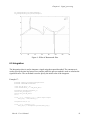
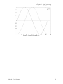
5.9.2 A simple example
The following is a simple example containing two equations to be solved. In this example, yn
designate the points calculated in curve yn(t), while y’n represent the first derivatives from the two
equations. The equation system to be solved is as follows:
y 0′ (t ) = 4 cos( y 0 (t )) + y1 (t ) +
3
1
t
y1′ (t ) = 4ty1 (t )
44
Microb – User’s Manual
Chapitre 5 : Vectmath
#include
#include
#include
#include
#include
#include
#include
#include
"../rk4.h"
"../euler.h"
<stdio.h>
<stdlib.h>
<assert.h>
<iostream.h>
<math.h>
"Vectmath/vectmath.h"
Vector fonct(double, Vector);
main()
{
int nb_equations = 2;
Vector initial(nb_equations);
Vector result_euler(nb_equations);
Vector result_RK4(nb_equations);
double pas = 0.00001;
int nb = 200000;
Euler euler;
RK4 rk4;
double t0 = 0;
// Number of equations to solve
// Initial conditions
Vector *p_fonc(double,Vector);
// Initialization of integration results and initial conditions
result_euler[0] = 0;
result_euler[1] = 0;
result_RK4[0] = 0;
result_RK4[1] = 0;
initial[0] = 2;
initial[1] = 1;
// Create function pointer
p_fonc = &fonct;
// Evaluate the results using the two integration methods
result_euler = euler.Compute(p_fonc, initial, t0, pas, nb, nb_equations);
result_RK4 = rk4.Compute(p_fonc, initial, t0, pas, nb, nb_equations);
// Print out results
printf( "Result of y1,
printf( "Result of y2,
printf( "Result of y1,
printf( "Result of y2,
integrated
integrated
integrated
integrated
using
using
using
using
euler: %f \n",result_euler[0]);
euler: %f \n", result_euler[1]);
runge-kutta: %f \n",result_RK4[0]);
runge-kutta: %f \n", result_RK4[1]);
}
Vector fonct(double t, Vector value)
{
int nb_equations = 2;
Vector yp(nb_equations);
double y0;
double y1;
y0 = valeur[0];
y1 = valeur[1];
yp[0] = 4*cos (y0) + pow(y1,3) + 1/(t+0.001);
yp[1] = 4*t*(y1);
return yp;
}
Microb – User’s Manual
45
Chapter 5 : Vectmath
5.10 Interaction between classes
5.10.1 Introduction
One of the major advantages of the Vectmath library is the interaction between the different classes
of objects. Examples include the multiplication of a matrix and vector, and the addition of a
rotation and a position-vector. Operator overloading was used as often as possible and in a way we
thought to be natural. Users should still pay attention and make sure that the behavior of an
operator applied to the classes is in fact what they are expecting.
5.10.2 Type conversion
Converting one type to another can be done in two days: by using the equal operator (=) or by type
casting. Table 2 lists the possible conversions by indicating the section where they are found. An X
means that the conversion cannot be done or does not have any specific properties.
Table 2: Type conversion
Vector
Matrix
5.10.2.1
Vector
Rotation
Transform
Position
Quaternion
Euler_angle
5.10.2.2
5.10.2.3
5.10.2.4
5.10.2.5
5.10.2.6
5.10.2.7
X
X
5.10.2.8
5.10.2.9
5.10.2.10
5.10.2.11
5.10.2.12.1
X
5.10.2.13.1
5.10.2.14.1
5.10.2.15.1
5.10.2.16.2
5.10.2.17.1
5.10.2.18.1
5.10.2.19.1
X
X
X
5.10.2.20.1
5.10.2.21.1
Rotation
X
Transform
X
5.10.2.12.2
5.10.2.8
X
5.10.2.16.1
Quaternion 5.10.2.9
5.10.2.13.2
5.10.2.17.2
X
Euler_angle 5.10.2.10
5.10.2.14.2
5.10.2.18.2
X
5.10.2.20.2
5.10.2.11
5.10.2.15.2
5.10.2.19.2
X
5.10.2.21.2
Position
Angle_axis
Angle_axis
5.10.2.22.1
5.10.2.22.2
5.10.2.1 Matrix and Vector
Vector to Matrix conversion is done without any loss of information. The process is as follows:
Matrix nrow x ncol becomes a Vector of 1 x ncol if ncol > nrow, otherwise it becomes a Vector of
nrow x 1.
Matrix A(4, 1);
Vector V;
A[0][0] = .5;
46
Microb – User’s Manual
Chapitre 5 : Vectmath
// V will be a row vector since A.nrow() > A.ncol()
V = A;
// Conversion using =
A = V;
((Matrix)R).print("Vector");
((Vector)A).print("A");
// Conversion by type casting
5.10.2.2 Matrix and Rotation
Rotation to Matrix conversion or vice versa is always done without any loss of information. Matrix
to Rotation conversion is only possible if a 3x3 Matrix is used.
Matrix A = mc_identity(3);
Rotation R;
A[0][0] = .5;
// NOTE: R may be other than orthonormal
R = A;
// Conversion by =
A = R;
((Matrix)R).print("R");
((Rotation)A).print("A");
// Conversion by type casting
5.10.2.3 Matrix and Transform
Matrix to Transform conversion or vice versa is always done without any loss of information.
Matrix to Transform conversion is only possible if a 4x4 Matrix is used.
Matrix A = mc_identity(4);
Transform T;
A[0][0] = .5;
A[0][3] = -1;
// NOTE: The T rotation part may be other than
// NOTE: orthonormal
T = A;
// Conversion by =
A = T;
((Matrix)T).print("T");
((Transform)A).print("A");
// Conversion by transtyping
5.10.2.4 Matrix and Position
Position to Matrix conversion is done without any loss of information. Matrix to Position
conversion can only be done if a 3x1 or 1x3 Matrix is used. In all cases, the type of vector (column
or row) is maintained.
Microb – User’s Manual
47
Chapter 5 : Vectmath
5.10.2.5 Matrix and Quaternion
Quaternion to Matrix conversion is done without any loss of information. Matrix to Quaternion
conversion is only done if a 4x1 or 1x4 Matrix is used. In all cases, the type of vector (column or
row) is maintained.
5.10.2.6 Matrix and Euler_angle
Euler_angle to Matrix conversion is done without any loss of information. Matrix to Euler_angle
conversion is done only if a 3x1 or 1x3 Matrix is used. In all cases, the type of vector (column or
row) is maintained.
5.10.2.7 Matrix and Angle_axis
Angle_axis to Matrix conversion is done without any loss of information. Matrix to Angle_axis
conversion is done only if a 6x1, 1x6, 7x1 or 1x7 Matrix is used. In all cases, the type of vector
(column or row) is maintained.
5.10.2.8 Vector and Position
Position to Vector conversion is done without any loss of information. Vector to Position
conversion is done only if a 3x1 or 1x3 Matrix is used. In all cases, the type of vector (column or
row) is maintained.
5.10.2.9 Vector and Quaternion
Quaternion to Vector conversion is done without any loss of information. Vector to Quaternion
conversion is only done if a 4x1 or 1x4 Matrix is used. In all cases, the type of vector (column or
row) is maintained.
5.10.2.10 Vector and Euler_angle
Euler_angle to Vector conversion is done without any loss of information. Vector to Euler_angle
conversion is only done if a 3x1 or 1x3 Matrix is used. In all cases, the type of vector (column or
row) is maintained.
48
Microb – User’s Manual
Chapitre 5 : Vectmath
5.10.2.11 Vector and Angle_axis
Angle_axis to Vector conversion is done without any loss of information. Vector to Angle_axis
conversion is only done if a 6x1, 1x6, 7x1 or 1x7 Vector is used. In all cases, the type of vector
(column or row) is maintained.
5.10.2.12 Rotation and Transform
5.10.2.12.1 From Rotation to Transform
The Transform consists of the rotation part (3x3 matrix located in the upper left-hand side) and a
nil position vector (3-element column vector located in the upper left-hand side). The 4th row is
made up of vector (0 0 0 1).

 R
[R] → 


0 0 0
0
0
0

1
5.10.2.12.2 From Transform to Rotation
The Rotation consists of the rotation part (3x3 matrix located in the upper left-hand side) of the
Transform.
P
 R
0 0 0 1  → [R ]


5.10.2.13 Rotation and Quaternion
5.10.2.13.1 From Rotation to Quaternion
The Rotation is converted into a Quaternion without any loss of information and so as to express
the same transformation in space. Note that each rotation may be represented by 2 quarternions (q
and q’).
5.10.2.13.2 From Quaternion to Rotation
Microb – User’s Manual
49
Chapter 5 : Vectmath
The Quaternion is converted into a Rotation without any loss of information and so as to express
the same transformation in space.
5.10.2.14 Rotation and Euler_angle
5.10.2.14.1 From Rotation to Euler_angle
The Rotation is converted into a Euler_angle without any loss of information and so as to express
the same transformation in space. Note that this conversion is not unique (i.e. a Rotation may yield
different Euler_angle vectors representing the same transformation).
5.10.2.14.2 From Euler_angle to Rotation
The Euler_angle is converted into a Rotation without any loss of information and so as to express
the same transformation in space.
5.10.2.15 Rotation and Angle_axis
5.10.2.15.1 From Rotation to Angle_axis
The Rotation is converted into an Angle_axis without any loss of information and so as to express
the same transformation in space.
5.10.2.15.2 From Angle_axis to Rotation
The rotation part of the Angle_axis is converted into a Rotation while the position part is lost.
5.10.2.16 Transform and Position
5.10.2.16.1 From Position to Transform
The Transform is made up of the identity rotation part (3x3 matrix located in the upper right-hand
side) and the position vector (3-element column vector located in the upper right-hand side). The
4th row is made up of vector (0 0 0 1).
50
Microb – User’s Manual
Chapitre 5 : Vectmath
1
0
[P] → 
0

0
0
1
0
0
0

0 P 

1

0 1
5.10.2.16.2 From Transform to Position
The Position is made up of the position part (3x1 vector located in the upper right-hand side) of the
Transform.
P
 R
0 0 0 1  → [P ]


5.10.2.17 Transform and Quaternion
5.10.2.17.1 From Transform to Quaternion
The rotation part of the Transform is converted into a Quaternion (see 6.10.2.13).
5.10.2.17.2 From Quaternion to Transform
The Quaternion is converted into a Rotation, then the latter is converted into a Transform (see
6.10.2.13).
5.10.2.18 Transform and Euler_angle
5.10.2.18.1 From Transform to Euler_angle
The rotation part of the Transform is converted into a Euler_angle (see 6.10.2.13).
5.10.2.18.2 From Euler_angle to Transform
The Euler_angle is converted into a Rotation, then the latter is converted into a Transform (see
6.10.2.13).
Microb – User’s Manual
51
Chapter 5 : Vectmath
5.10.2.19 Transform and Angle_axis
5.10.2.19.1 From Transform to Angle_axis
The Transform is converted into an Angle_axis without any loss of information.
5.10.2.19.2 From Angle_axis to Transform
The Angle_axis is converted into a Transform without any loss of information.
5.10.2.20 Quaternion and Euler_angle
5.10.2.20.1 From Quaternion to Euler_angle
The Quaternion is converted into a Euler_angle without any loss of information and so as to
express the same transformation in space. Note that this conversion is not unique (i.e. a Quaternion
may yield different Euler_angle vectors representing the same transformation).
5.10.2.20.2 From Euler_angle to Quaternion
The Euler_angle is converted into a Quaternion without any loss of information and so as to
express the same transformation in space.
5.10.2.21 Quaternion and Angle_axis
5.10.2.21.1 From Quaternion to Angle_axis
The Quaternion is converted into Angle_axis without any loss of information and so as to express
the same transformation in space.
5.10.2.21.2 From Angle_axis to Quaternion
The rotation part of the Angle_axis is converted into a Quaternion while the position part is lost.
5.10.2.22 Euler_angle and Angle_axis
5.10.2.22.1 From Euler_angle to Angle_axis
52
Microb – User’s Manual
Chapitre 5 : Vectmath
The Euler_angle is converted into Angle_axis without any loss of information and so as to express
the same transformation in space.
5.10.2.22.2 From Angle_axis to Euler_angle
The rotation part of the Angle_axis is converted into an Angle_axis while the position part is lost.
5.10.3 Operations involving different classes
An object from a given class that expresses pure rotation in space (Rotation, Quaternion,
Euler_angle) may be combined with a Position using a + operator to create an object from a class
that expresses an orientation and a position (Transform or Angle_axis):
(Transform) T = (Rotation) R + (Position) P;
(Transform) T = (Quaternion) Q + (Position) P;
(Transform) T = (Euler_angle) E + (Position) P;
(Angle_axis) A = (Rotation) R + (Position) P;
(Angle_axis) A = (Quaternion) Q + (Position) P;
(Angle_axis) A = (Euler_angle) E + (Position) P;
5.10.4 Examples of interaction between classes
Exemple 10 : Creating a rotation
Euler_angle E(.75, -1.57, 0.0);
Rotation R = E;
Rotation R = Angle_axis(.4, 5, 6, 1, 2, 3);
Exemple 11 : Creating a Transform
Position P(.3, -1.2, .04);
Quaternion Q(0.741713, -0.130604, 0.594085, 0.282607);
Transform T = Q + P;
Transform T2 = Euler_angle(1, -2, 3) + Position(3, 4, 5);
Transform T3 = Angle_axis(.2, 4, 3.4, 4, 5, 6);
Transform T4 = Angle_axis(4, 1, 0, 0, 4, 5, 6);
Exemple 12 : Extracting the rotation part of a Transform
Position P1(1, 2, 3);
Position P2(.5, 1.2, 3.4);
Euler_angle E(0, 1.57, -1.57);
Transform T1 = E + P1;
// Create T2 made up of the rotation part of T1 and P2
Transform T2 = (Rotation)T1 + P2;
Microb – User’s Manual
53
6
Signal_processing
The Signal_processing library has classes that process data. This is especially useful when the robot
is equipped with sensors with noisy input (e.g. potentiometer, force sensor) or for control
algorithms (e.g. integrators, differentiators, etc.). The available classes are: Mean, Median,
Butterworth, Derivative, Integration and Lagrange_der. The classes can process one signal at a time
or a group of signals, as will be shown further on. As the classes process temporal data, they will
introduce a time lag that is proportional to the size of the operation used.
6.1 Mean filter
The Mean class implements a filter that returns the mean value among the last N values provided.
In the example that follows, we will be using the mean filter to attenuate noise on a sinusoidal
signal. The signal contains 128 data while the filter has a width of 5. The constructor is used to
specify the width of the filter while the process method is used for the actual filtering.
Exemple 13 :
#include "Signal_processing/mean.h"
#include "Vectmath/vectmath.h"
const int nb_data = 128;
const int filter_width = 5;
Mean mean(filter_width);
Vector data_in(nb_data);
Vector data_out(nb_data);
int i;
for(i = 0; i < nb_data; ++i) // Create the input signal
{
data_in[i] = sin(i*2*M_PI/nb_data);
// Add a step in the middle of the signal...
if(i > nb_data/2) data_in[i] += 1.5;
}
// ... and two pulses
data_in[nb_data/5] += 2.0;
data_in[nb_data*3/4] -= 3.5;
for(i = 0; i < nb_data; ++i)
data_out[i] = mean.process(data_in[i])
mc_transpose(data_in).print("Input");
mc_transpose(data_out).print("Output");
Microb – User’s Manual
55
Chapter 6 : Signal_processing
Figure 2 : Effect of mean filter
6.2 Median filter
The Median class implements a filter that returns the median value among the last N values
provided. This filter behaves similarly to a mean filter but its advantage is that it maintains the
“steps” while eliminating short-duration pulses. In the example that follows, the median filter will
be used to eliminate noise from a sinusoidal signal. The signal contains 128 data while the filter has
a width of 5. The constructor is used to specify the width of the filter while the process method is
used for the actual filtering.
Exemple 14 :
#include "Signal_processing/median.h"
#include "Vectmath/vectmath.h"
const int nb_data = 128;
const int filter_width = 5;
Median median(filter_width);
Vector data_in(nb_data);
Vector data_out(nb_data);
int i;
for(i = 0; i < nb_data; ++i)
// Create input signal
{
data_in[i] = sin(i*2*M_PI/nb_data);
// Add a step in the middle of the signal...
56
Microb – User’s Manual
Chapitre 6 : Signal_processing
if(i > nb_data/2) data_in[i] += 1.5;
}
// ... and two pulses
data_in[nb_data/5] += 2.0;
data_in[nb_data*3/4] -= 3.5;
for(i = 0; i < nb_data; ++i)
data_out[i] = median.process(data_in[i])
mc_transpose(data_in).print("Input");
mc_transpose(data_out).print("Output");
Figure 3 : Effect of median filter
6.3 Butterworth filter
Microb also has a class that allows data to be filtered using a Butterworth filter. The Butterworth
filter is a filter where all the poles are located on a half-circle with a radius of 1 in the left-hand
complex half-plane. The Butterworth class requires discretized transfer function coefficients
obtained from the desired cutoff frequency and the filter order. These coefficients may be found
using a software program such as Octave (e.g. [b, a] = butter(2, 0.09)) and must be specified when
the constructor is called up. The filter is then used in the same way as the median filter shown in
the previous example.
Microb – User’s Manual
57
Chapter 6 : Signal_processing
Exemple 15 :
#include "Signal_processing/butterworth.h"
#include "Vectmath/vectmath.h"
const int nb_data = 32;
const int filter_width = 3;
// Cutoff frequency of 0.09, order 2
Vector3 a(0, -1.6041, 0.6705);
Vector3 b(0.0166, 0.0332, 0.0166);
Butterworth butterworth(filter_width, a, b);
Vector data_in(nb_data);
Vector data_out(nb_data);
int i;
for(i = 0; i < nb_data; ++i) // Create input signal
{
data_in[i] = sin(i*2*M_PI/nb_data);
// Add a step in the middle...
if(i > nb_data/2) data_in[i] += 1.5;
}
// ...and two pulses
data_in[nb_data/5] += 2.0;
data_in[nb_data*3/4] -= 3.5;
for(i = 0; i < nb_data; ++i)
data_out[i] = median.process(data_in[i])
mc_transpose(data_in).print("Input");
mc_transpose(data_out).print("Output");
6.4 Lagrange derivative
The Derivative class is a Lagrange derivative filter of width 3. The constructor is used to specify
the time lag between two samples while the process method is used to calculate the signal
derivative.
Exemple 16 :
#include "Signal_processing/derivative.h"
#include "Vectmath/vectmath.h"
const int nb_data = 32;
const double delta_t = 2*M_PI/nb_data;
Derivative derivative(delta_t);
Vector data_in(nb_data);
Vector data_out(nb_data);
int i;
for(i = 0; i < nb_data; ++i) // Create input signal
data_in[i] = sin(i*delta_t);
for(i = 0; i < nb_data; ++i)
data_out[i] = derivative.process(data_in[i])
58
Microb – User’s Manual
Chapitre 6 : Signal_processing
mc_transpose(data_in).print("Input");
mc_transpose(data_out).print("Output");
Figure 4 : Effect of Butterworth filter
6.5 Integration
The Integration class is used to integrate a signal using the trapezoid method. The constructor is
used to specify the time lag between two samples while the process method is used to calculate the
signal derivative. The set method is used to specify the initial value of the integrator.
Exemple 17 :
#include "Signal_processing/integration.h"
#include "Vectmath/vectmath.h"
const int nb_data = 32;
const double delta_t = 2*M_PI/nb_data;
Integration integration(delta_t);
Vector data_in(nb_data);
Vector data_out(nb_data);
int i;
for(i = 0; i < nb_data; ++i) // Create input signal
data_in[i] = sin(i*delta_t);
integration.set(-1.0);
for(i = 0; i < nb_data; ++i)
data_out[i] = integration.process(data_in[i])
Microb – User’s Manual
59
Chapter 6 : Signal_processing
mc_transpose(data_in).print("Input");
mc_transpose(data_out).print("Output");
Figure 5 : Effect of Lagrange derivative
6.6 Multiple signal processing
Users may wish to process a signal with multiple dimensions (e.g. the values of a robot’s
potentiometers). The functions mc_new_mean, mc_new_median, mc_new_butterworth and
mc_new_derivative are used to allocate a list of operations of variable length. The following
example shows how this function is used for a 6-element vector. Certain parts of the code have
been omitted for the sake of clarity.
Exemple 18 :
...
Mean *p_mean(filter_width);
p_mean = mc_new_median(6, nb_data);
Matrix data_in[6][nb_data];
Matrix data_out[6][nb_data];
...
for(i = 0; i < nb_data; ++i)
for(j = 0; j < 6; ++j)
data_out[j][i] = p_mean[j].process(data_in[j][i])
...
60
Microb – User’s Manual
Chapitre 6 : Signal_processing
Figure 6 : Result of Exemple 18 :
Microb – User’s Manual
61
7
Configuration
The Configuration library is used to read and write configuration files. It is also used to extract
configuration subsets. The configuration files used to provide the parameters of a given robot are
presented in section 1.
Configuration files are made up of parameters and comments. A comment is a line that begins with
the number sign (#). These lines are ignored when the file is read. Parameters are made up of four
parts: a label, a type, a string of characters, and data, which vary based on the type (MC_MATRIX
or MC_LIST). The following figure shows the different parts that make up a parameter.
Type du paramètre
Étiquette du paramètre
Chaîne de caractère
Matrices de données
Group.name:MC_MATRIX {
[String]
2 3
Dimensions de la matrice
1 2 3
4 5 6
}
Figure 7: Definition of a parameter
7.1 Label
The label defines the name of the parameter. It begins the definition of a parameter and is made up
of one or more words separated by a period. The convention used for Microb is that the first word
represents the class for which the parameter is intended, while the second word is the name of the
attribute where the parameter will be stored. For instance, the parameter Robot.base is used to
initialize the basic attribute of the Robot class. It is recommended that users use the same
convention for attributes specific to their robots.
7.2 Type
The type, which is optional, is located immediately after the label and specifies the nature of the
parameter. When there is a type, a colon (:) is used to separate the label from the type. Two types
are currently supported: MC_MATRIX and MC_LIST. The default type is MC_MATRIX.
Microb – User’s Manual
63
Chapter 7 : Configuration
7.3 Character string
The character string is used to insert a comment that is to remain with the parameter (not to be
confused with the comments that begin with the number sign (#), which are not read). The
character string is marked off by brackets ([ ]).
7.4 Data
7.4.1 MC_MATRIX
The data matrix is made up of two dimensions and data. The two dimensions are the number of
rows and the number of columns.
Exemple 19 :
Robot.HD:MC_MATRIX {
[example]
2 4
1 2 3 4
4 5 6 7
}
7.4.2 MC_LIST
The data are made up of a set of character strings. The first word in each string serves as an index
to reference the string.
Exemple 20 :
Server.script:MC_LIST {
[other example]
length 1
weight 10.3
name Test
Comment This is a test
}
7.5 Reading a file
To read a configuration file, the filename is entered when the constructor is called up, or the read
method is used.
#include "Configuration/configuration.h"
Configuration conf("file.cnf");
64
Microb – User’s Manual
Chapitre 7 : Configuration
or
#include "Configuration/configuration.h"
Configuration conf;
conf.read("file.cnf");
7.6 Obtaining a parameter
The get_comments, get_matrix and get_list methods are used to obtain the comment, matrix and list
of one parameter.
char *string = conf.get_comments("HD.convention");
Matrix mat = conf.get_matrix("Robot.base");
List *list = conf.get_list("Server.script");
Users can also check whether an element is found in the configuration with the item_exists method.
if(conf.item_exists("Robot.tool_mount"))
tool_mount = conf.get_matrix("Robot.tool_mount");
The get_matrix(Conf_item*) method is more efficient by avoiding having to search through the list
twice.
tool_mount = conf.get_matrix(item, x, y, Configuration::Error);
7.7 Obtaining a subset
The Configuration class is used to group the parameters into subsets to increase the efficiency of
the search and the coherence of the configuration file.
For instance, let’s assume that the conf::Configuration object contains the following parameters:
HD.a
HD.d
HD.alpha
HD.theta
Robot.base
Robot.tool_mount
Robot.velocity_max
The get_configuration method is used to extract the two subsets HD and Robot.
Configuration hd_conf = conf.get_configuration("HD");
Matrix a = hd_conf.get_matrix("a");
Matrix d= hd_conf.get_matrix("d");
Configuration robot_conf = conf.get_configuration("Robot");
Matrix base = robot_conf.get_matrix("base");
Microb – User’s Manual
65
Chapter 7 : Configuration
7.8 Robot configuration
The Mobile_robot and Serial_robot classes used to define a robot contain a configuration-type
attribute known as conf. The read method from the Mobile_robot class calls up the Kinematic read
method, which calls up the HD read method, which in turn calls up the read method of the conf
attribute, after which it initializes some of its attributes to the values of the configuration file
parameters. The read method used for derivative classes also initializes certain attributes. Users
may, if they wish, include their own parameters in the configuration file and overload the read
method of the Serial_robot. However, they must directly call up (Serial_robot::read()) to ensure
that the other classes have been properly initialized. Parameter initialization is similar for mobile
robots. It is recommended to use the robot’s name as prefix in the configuration file to ensure that
the file is clear (e.g. Puma760.enc_offset).
66
Microb – User’s Manual
8
Robot
The Robot module (along with the Control and Controllers modules) is the very essence of Microb.
The Robot module is used to define a robot using its HD parameters, direct and inverse kinematics,
dynamics, etc.
8.1 HD class
The HD class (for Hartenberg and Denavit) is used to define the kinematic properties of serial
robots. Most of the attributes of this class are defined using a robot’s configuration file (see section
1). The read method is used to read a configuration file and initialize the attributes. The print
method is used to display the class values. These values will be used by the Kinematic and
Serial_robot classes as well as the class which inherits from them.
Note that Microb supports two versions of the HD convention, i.e. Paul and Craig. The
HD.convention parameter is used to define the version used in the file. Microb uses the Paul
version by default.
Exemple 21 :
HD hd;
hd.read("Puma760.cnf");
hd.print();
Users do not usually have to call up the read method of the HD class directly since it is overloaded
by the Serial_robot class.
8.2 Kinematic class
This class provides direct and inverse kinematic generic functions for serial robots. Direct
kinematics can be used for any type of serial robot, while inverse kinematics are used for serial six
DOF wrist-partitioned robots. In the following example, a Kinematic-type object is declared, which
is initialized using a configuration file. During normal Microb use, users do not need to handle this
class directly (this is a basic class which Serial_robot inherits).
Exemple 22 :
Kinematic kin("Puma760.cnf");
Microb – User’s Manual
67
Chapter 8 : Robot
Vector6 v(-1.57 0 -3.14 0 1.57);
v.print("Initial joint values");
kin.set_theta(v);
Transform T = kin.get_Q();
T.print("Direct kinematics ");
v = kin.inverse(T);
v.print("Inverse kinematics");
For robots which do not have six degrees of freedom or which are not wrist-partitioned, users must
overload the inverse kinematic methods if they wish to use a controller that requires this function
(cartesian controllers). Users may also wish to overload the inverse and direct kinematic methods in
order to optimize calculations as required.
8.3 Robot class
The Robot class uses all the parameters that apply to all the robots in the configuration object. This
class is designed to simplify the user interface since all users must use the terminology used in this
class and the terminology applies to all serial and mobile robots. In addition, this convention is
used in the design of generic controllers.
8.4 Serial_robot class
The Serial_robot class inherits from the Robot, Kinematic and HD classes. It uses the HD
parameters to overload the methods related to the generalized coordinates. In short, it creates the
gen_coord vector by using theta for the rotary joints and d for the prismatic joints. It also checks
the joint boundaries by taking into account the nature of each joint.
Exemple 23 :
Serial_robot my_robot("Puma760.cnf");
Vector6 v(-1.57, 0, -3.14, 0, 1.57);
v.print("Initial joint values");
my_robot.set_gen_coord(v);
Transform T = my_robot.get_Q();
T.print("Direct kinematics");
v = my_robot.inverse(T);
v.print("Inverse kinematics");
68
Microb – User’s Manual
Chapitre 8 : Robot
8.5 Mobile_robot class
The Mobile_robot class performs operations similar to those of the Serial_robot class. However,
the generalized coordinates in this case are defined by cartesian degrees of freedom.
8.6 Wheeled_robot class
The Wheeled_robot class contains conventions for the terminology used to design generic
controllers for wheeled mobile robots. In more concrete terms, these conventions take the form of
direct and inverse kinematic virtual methods and I/Os for the position of each wheel.
8.7 Rigid_body class
The Rigid_body class contains the parameters required to define a mobile robot, which can be seen
as a rigid body of arbitrary shape moving in cartesian space (see the document on the underwater
inspection controller for more information on these concepts). This class is used to calculate the
forces and moments shared by all rigid bodies and determine their position in space. It is thus
possible to use the Rigid_body class to model any type of mobile robot without any non-holonomic
constraints. For a specific application (which should normally contain a controller and motor) able
to use a virtual model, the Rigid_body class consists in creating a derived class which models the
forces and moments which must be added to those already present in the base class. For instance,
for a helicopter model, the forces and moments generated by the helicopter’s blades will have to be
calculated, as well as those caused by the motion of the air (drag and lift) and added to those
calculated by Rigid_body.
The main Rigid_body methods used to calculate the forces and moments and to position the body
in space are model_integration(), kinematic_model(), dynamic_model(), compute_gravity() and
compute_inertial_dynamic_forces().
The compute_gravity() and compute_inertial_dynamic_forces() methods are used to calculate the
forces that act on all rigid bodies. First, compute_gravity() calculates the force of gravity, then
compute_inertial_dynamic_forces() calcules the inertial forces and moments which act on the body
due to its mass, as well as the moments due to the Coriolis force. Note that it is possible to include
coefficients of mass added to the inertia matrix (when reading the configuration file) to model
certain additional forces acting on the body.
The kinematic_model() and dynamic_model() methods respectively correspond to the rigid body’s
kinematic and dynamic models. The kinematic model uses the quarternion law of propagation and
the derivative of the position vector in the local reference frame to determine the body’s velocities
in the local reference frame. The dynamic model uses the F = ma and I = Mθ&& laws to determine
Microb – User’s Manual
69
Chapter 8 : Robot
the body’s acceleration. To do so, an inertia matrix must be correctly initialized and inverted,
which is done when reading the configuration file. In addition, to the forces and moments
calculated by Rigid_body (in the compute_gravity() and compute_inertial_dynamic_forces()
methods) are added those specific to the derived class model. The derived class must use the
variable gen_forces to transmit these values to Rigid_body. The variable gen_forces is a 6-element
vector with the following form:
[N
x
Ny
Nz
Fx
Fy
Fz
]
where all the values are measured in the local reference frame.
The derived class must call up the model_integration() method at each control loop iteration. This
method uses the forces calculated by the basic class and the additional forces included in
gen_forces in order to calculate the accelerations and velocities (angular and linear) and the body’s
position. It performs a dual integration by using the 4th order Runge-Kutta integration method
provided by Microb. The methods that define the acceleration and velocity equations for purposes
of using the Runge-Kutta method are respectively dynamic_equation() (which calls up
dynamic_model()) and kinematic_equation() (which calls up kinematic_model()). The
accelerations, velocities and body position are all measured in the local reference frame (attached to
the body).
The following are the main operations that need to be done for the derived class:
•
Initialize the rigid body parameters: call up Rigid_body::read() and add the parameters to the
configuration file (inertia matrix, position of the centre of mass and initial conditions).
•
Calculate the external forces acting on the body: at each iteration, calculate the forces and
moments originating from the motors, etc. and include them in gen_forces.
•
Update the accelerations, velocities, and position of the body: at each iteration, call up the
model_integration() method.
70
Microb – User’s Manual
9
Control
The Control module contains the trajectory generators. It includes three types of trajectories. The
Trajectory class discretizes a given value and is used for trajectories in the joint domain.
CTrajectory is used for the Cartesian domain. The ETrajectory class is used to define elliptical
trajectories.
The set_from and set_target methods are used to specify the starting and ending points, while the
get_next_pose method gives intermediate values. The joint or cartesian movements follow a
velocity profile with a trapezoid shape (acceleration, constant velocity, deceleration). The velocity
profile is determined by the maximum velocities and maximum accelerations which must be
defined using the set_max_speed and set_max_accel methods. For elliptical trajectories, a pose
must be specified for the starting point and ending point, as well as for an intermediate point.
It is always preferable to use a trajectory generator in robotics applications. Otherwise, the gains
need to be modified based on the desired specifications. For instance, the response time (tr)
increases with the gains module. Trajectory generation frees up part of the work to the PID
compensator. The trajectory generator requires the robot to follow a trajectory by constantly
moving in small increments (D) to reach the desired pose (see Figure 9). The compensator gains
can thus be adjusted to obtain an acceptable response time (tr) and overtravel (d) for this type of
motion. The time required to attain the final desired pose is then adjusted by selecting the
maximum velocity and acceleration. The overall performance is also improved since the robot
decelerates before reaching the desired pose.
9.1 Trajectory generation in the joint domain
When in the joint domain, the number of joints must be specified in the constructor. The methods
set_from, set_target, set_max_speed and set_max_accel use as arguments vectors with units
associated with the joint domain (usually rad, rad/sec and rad/sec2).
#include "Control/traj.h"
#include "Vectmath/vectmath.h"
Trajectory traj(4);
const double period = .5;
Vector4 V0(0, 0, 1.57, -1.57);
Vector4 V1(1.57, 1.57, 1.9, 0);
Vector4 V = V0;
// sec
// rad
// rad
traj.set_from(V0);
traj.set_target(V1);
Microb – User’s Manual
71
Chapter 9 : Control
Vector4 v_max(1, .5, 1, 2);
Vector4 a_max(2, 2, 2, 3);
// rad/sec
// rad/(sec*sec)
traj.set_max_speed(v_max);
traj.set_max_accel(a_max);
mc_transpose(V).print();
while(!traj.done())
{
V = (Vector4) traj.get_next_pose(period);
mc_transpose(V).print();
}
9.2 Trajectory generation in the Cartesian domain
In the Cartesian domain, no elements need to be specified when calling up the constructor. The
set_from and set_target methods use Transforms as arguments. The set_max_speed and
set_max_accel methods use vectors with units related to the Cartesian domain as arguments
(rad/sec, rad/sec, rad/sec, m/sec, m/sec, m/sec) and (rad/sec2, rad/sec2, rad/sec2, m/sec2, m/sec2,
m/sec2).
#include "Control/ctraj.h"
#include "Vectmath/vectmath.h"
CTrajectory ctraj;
const double period = .5;
// sec
Transform T0 = Euler_angle_xyz(0, 0, 0, 1, 2, 3);
Transform T1 = Euler_angle_xyz(1.57, 0, 3.14, 0, 3, -4);
Angle_axis_xyz A = T0;
ctraj.set_from(T0);
ctraj.set_target(T1);
Vector6 v_max(1, 1, 1, 2, 2, 2);
Vector6 a_max(2, 2, 2, 3, 3, 3);
// rad/sec and m/sec
// rad/(sec*sec) and m/(sec*sec)
ctraj.set_max_speed(v_max);
ctraj.set_max_accel(a_max);
mc_transpose(A).print();
while(!ctraj.done())
{
A = ctraj.get_next_pose(period);
mc_transpose(A).print();
}
Note that even if there is a discontinuity in the desired accelerations due to the velocity trapezoid in
the generation of trajectories, there will be no problems with an actual robot since the robot’s actual
trajectory does not contain any unevenness.
9.3 Generation of elliptical trajectories
#include "Control/Etraj.h"
#include "Vectmath/vectmath.h"
void generate(Transform &p1, Position &p2, Transform &p3)
{
p1 = mc_Rz(-1);
p3 = mc_Rz(2);
72
Microb – User’s Manual
Chapitre 9 : Control
p1[0][3] = 14.0; p1[1][3] = 18.0; p1[2][3] = 4.0;
p2[0]
= 16.0; p2[1]
= 8.0; p2[2]
= 5.0;
p3[0][3] = -3.0; p3[1][3] = -6.0; p3[2][3] = 0.0;
}
int main(int, char**)
{
ETrajectory etraj;
const double period = .5;
Transform T0,T1;
Position p;
generate(T0, p, T1);
Angle_axis_xyz A = T0;
etraj.set_from(T0);
etraj.set_middle_target(p);
etraj.set_target(T1);
Vector3 v_max(4, 4, 4);; // rad/sec et m/sec
Vector3 a_max(1, 1, 1); // rad/(sec*sec) et m/(sec*sec)
etraj.set_max_speed(v_max);
etraj.set_max_accel(a_max);
mc_transpose(A).print();
while(!etraj.done())
{
A = etraj.get_next_pose(period);
mc_transpose(A).print();
}
return(1);
}
9.4 PID Compensator
The Control module also contains a PID compensator. The gains for each type of control may be
configured separately. The PID class performs the numerical derivative and integral on the signal
using the Signal_processing module which includes these functions. To not use the integral torque,
the gain should be left at 0. There is also a function for using a threshold on the integrator.
Moreover, the compensation method is overloaded to act on doubles, Vectors, Quaternions or
Quaternion_xyzs. Based on the type of parameter passed to the get_command method, the
compensation will take place in the joint or Cartesian domain. In the latter case, the error used in
the algorithm is calculated using the quaternion theory.
9.5 Compensator for adaptive control
The Adaptive module contains the adaptation law which calculates the value of the parameters to
be calibrated on line. The method that calculates the value of these parameters must be called up at
each iteration of the control using the module. Other methods can also be used to enter the initial
estimated values of the parameters, the gains from the adaptation law, etc.
Microb – User’s Manual
73
10
Exception Handling
Microb uses the exception handling function from C++ based on the concept of the try and catch
blocks and the throw operator. When an exception occurs in a library, an object is “thrown” and the
application is responsible for “catching” it. If no catch block takes care of the problem, the
application ends with an error message. This situation is not desirable in a robot control context.
10.1 Error objects
When an error occurs in Microb, an object representing the type of error is launched. The object
also contains a message providing information on the error that occurred. The object classes are
defined in the OSDL/error_handling.h file. The classes are Generic_error, Warning and
Fatal_error. The Generic_error class is a basic class from which other classes inherits. The print
method for these classes is used to display the message contained in the object, while the
get_error_type and get_message methods return the type of error and the message, respectively.
10.2 Try and catch blocks
To catch one of the error objects, the code must be placed where the error may occur in a try block
(set off by brackets).
Following the block, one or more catch blocks must be placed. The catch operator uses as argument
the type of error which the user wishes to catch and a name for the object (optional). The block is
also set off by brackets. The user may place more than one catch block after a try block; only the
first catch block with a type that corresponds to that of the error (or to one of its basic types) will be
executed.
The following code provides a simple example of exception handling. The line contained in the try
block attempts to add two matrix classes with different dimensions. The + operator will detect the
problem and launch a Fatal_error object. As this object inherits from Generic_error, the catch block
(Generic_error error) will catch the object. The object’s print method is called up to display the
error message.
Exemple 24 :
#include "Vectmath/vectmath.h"
#include "OSDL/error_handling.h"
Microb – User’s Manual
75
Chapter 10 : Exception Handling
Transform T = mc_identity(4);
Vector3 v(1, 2, 3);
Matrix m;
try
{
m = T + v;
// Incompatible type
}
catch(Generic_error error)
{
error.print();
}
The following is another example where several catch blocks are used to handle errors. Note that
the last catch(...) block catches all of the errors that were not handled.
Exemple 25 :
#include "Vectmath/vectmath.h"
#include "OSDL/error_handling.h"
Transform T = mc_identity(4);
Vector3 v(1, 2, 3);
Matrix m;
try
{
m = T + v;
// Incompatible type
}
catch(Warning error)
{
error.print();
}
catch(Fatal_error error)
{
error.print();
exit(-1);
}
catch(Generic_error error)
{
error.print();
exit(-1);
}
catch(...)
{
printf("Unknown error\n");
exit(-1);
}
In the above examples, only one line was contained in the try block. In normal applications, several
lines will be included that may even contain function calls. In fact, a single try block may be used
for any application for all exception handling.
76
Microb – User’s Manual
Appendice 1 - Configuration Files
When users wish to control a new manipulator with the Microb library, they need to first define the
robot’s physical properties using parameters. Each parameter is identified by a specific label. Some
of these parameters are mandatory while others are optional. They are designed to initialize certain
class attributes related to the robot. The table below presents the configuration parameters used by
Microb.
Table 2 – Configuration parameters
Parameters
Dimensions
Unit
Description/note
HD.a
HD.nb_gen_coord x 1
m
HD a parameters
HD.d
HD.nb_gen_coord x 1
m
HD d parameters
HD.alpha
HD.nb_gen_coord x 1
degree
HD alpha parameters
HD.theta
HD.nb_gen_coord x 1
degree
HD theta parameters
HD.d_min
HD.nb_gen_coord x 1
m
Upper boundaries of d (if type = Prismatic)
HD.d_max
HD.nb_gen_coord x 1
m
Lower boundaries of d (if type = Prismatic)
HD.conv
Convention: Paul or Craig
Robot.type
HD.nb_gen_coord x 1
Type of joint: 0 -> Angular or 1 -> Prismatic
Robot.nb_gen_coord
1x1
Size of generalized coordinate vector
Robot.nb_gen_forces
1x1
Size of generalized force vector
Robot.gen_coord_min
HD.nb_gen_coord x 1
degrees
Lower boundaries of generalized coordinates (if type =
Angular)
Robot.gen_coord_max
HD.nb_gen_coord x 1
degrees
Upper boundaries for generalized coordinates (if type =
Angular)
Robot.base
6x1
(degrees, m)
Transform between the robot base and starting
referential for the HD convention
Robot.world
6x1
(degrees, m)
Transform between the world referential and robot base.
Robot.tool_mount
6x1
(degrés, m)
Transform between the last referential and the location
where the tool is installed. It is the end-effector which
cannot be described using Craig’s HD convention and
which cannot always be fully described using Paul’s
convention.
Robot.master_slave
Microb – User’s Manual
Type of robot 0 for master-slave, 1 for slave and 2 for
master
77
Chapter 10 : Exception Handling
Robot.gen_forces_limit
HD.nb_gen_coord x 1
n-m
Maximum generalized force which can be sent to each
joint
Robot.flag_feedback
1x1
NO_FEEDBACK, PD_NUM, I_NUM or PID_NUM
(defined in Robot/robot.h)
Robot.flag_dynamic
1x1
NO_DYNAMIC, STATIC_FORCES,
INV_DYN_MODEL_BASED,
INV_DYN_MESURED_FORCES ou
INV_DYN_ADAPTATIVE (defined in Robot/robot.h)
Robot.gen_coord_error_max HD.nb_gen_coord x 1
degrees
Maximum allowable error for each joint
Robot.velocity_max
HD.nb_gen_coord x 1
degrees/sec
Maximum allowable velocity for each joint
Robot.acceleration_max
HD.nb_gen_coord x 1
degrees/sec2 Maximum allowable acceleration for each joint
Graph.draw
HD.nb_gen_coord x 3
Whether the links A, D and the joints are drawn or not
Graph.link_color
HD.nb_gen_coord x 3
Link color
Graph.joint_color
HD.nb_gen_coord x 3
Joint color
Graph.link_diameter
HD.nb_gen_coord x 1
m
Link diameter
Graph.joint_diameter
HD.nb_gen_coord x 1
m
Joint diameter
Graph.type_link
HD.nb_gen_coord x 1
78
0 -> cylinder shape, 1 -> box shape
Microb – User’s Manual
Appendice 2 - Class Diagram
Microb – User’s Manual
79
Chapter 10 : Exception Handling
Index
A
Adaptative, 65
aléatoire, génération de nombre, 16
Angle_axis, 36
B
Butterworth, 49
C
Chronomètre, 10
Client, 17
compensateur PID, 65
Configuration, 55
Control, 63
contrôle adaptatif, 65
CTrajectory, 63
D
Derivative, 50
dérivée, 50
E
Engine, 13
périodicité, 14
équations différentielles, intégration, 38
erreurs, traitement des, 67
ETrajectory, 63
Euler_angle, 35
exceptions, 67
F
filtre
de Butterworth, 49
dérivatif, 50
médian, 48
moyenneur, 47
H
HD, 59
I
Intégration, 51
K
Kinematic, 59
L
List, 17
M
maître de poste, 7
Maître de poste, 9
matrice
initialisation, 23
matrices
analyse, 24
création, 23
opérations, 23
Matrix, 22
mc_random, 16
mc_seed, 16
Mean, 47
Median, 48
Mémoire partagée, 16
P
PID, 65
Position, 31
Q
Quaternion, 33
R
Record, 18
80
Microb – User’s Manual
Chapitre 10 : Exception Handling
Rigid_body, 61
robot
mobile, 60
mobiles à roues, 60
sériel, 60
Robot, 59
Rotation, 28
S
Sandglass, 10
Semaphore, 11
Serial_robot, 60
Server, 17
Shmem, 16
Signal_processing, 47
Socket, 7
Microb – User’s Manual
T
Thread, 12
traitement de signal, 47
trajectoire, génération de
domaine articulaire, 63
domaine cartésien, 64
elliptique, 64
Trajectory, 63
Transform, 29
U
Utilities, 17
V
vecteur, 26
Vectmath, 21
conversion de types, 40
Vector, 26
81