Download Bauer060825 - Centre for Intelligent Machines

Diploma Thesis
The Development and
Implementation of Kinematics
Algorithms on RVS (Robot
Visualization System)
Frank Bauer
August 25, 2006
Fachhochschule Münster
Abteilung Steinfurt
Fachbereich Maschinenbau
Erklaerung
“Hiermit erklaere ich, die Diplomarbeit selbststaendig verfasst und keine anderen als
die angegebenen Hilfsmittel verwendet zu haben.”.
Brilon, August 25, 2006
Frank Bauer
Abstract
This report describes the development of a computer program for the simulation of
robots. The program is called Robot Visualization System (RVS) 2006 and is based on
a software package, also called RVS, that was developed over 10 years ago. Because
the original RVS was adapted to a Silicon Graphics Workstation, the software is not
compatible to current computer architectures. Therefore, the source code of RVS
needs to be modified in order to use the tool on an IBM-compatible PC. The aim of
this report is to document all steps that are required for this task.
Zusammenfassung
in deutsch
Contents
1 Introduction
1.1 Introduction . . . .
1.2 Robot Visualization
1.3 Using RVS . . . . .
1.4 Objectives . . . . .
.
.
.
.
1
1
2
2
2
2 Overview of RVS
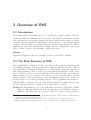
2.1 Introduction . . . . . . . . . . . . . . . . . . . . . . . . . . . . . . . . .
2.2 The Main Structure of RVS . . . . . . . . . . . . . . . . . . . . . . . .
4
4
4
. . . . .
System
. . . . .
. . . . .
3 User Interface
3.1 Separation of the Project
3.2 Graphics Library . . . .
3.3 Graphical User Interface
3.4 How FLTK works . . . .
3.5 OpenGL in FLTK . . . .
.
.
.
.
.
.
.
.
.
.
.
.
.
.
.
.
.
.
.
.
.
.
.
.
.
.
.
.
.
.
.
.
.
.
.
.
.
.
.
.
.
.
.
.
.
.
.
.
.
.
.
.
.
.
.
.
.
.
.
.
.
.
.
.
.
.
.
.
.
.
.
.
.
.
.
.
.
.
.
.
.
.
.
.
.
.
.
.
.
.
.
.
.
.
.
.
.
.
.
.
.
.
.
.
.
.
.
.
.
.
.
.
.
.
.
.
.
.
.
.
.
.
.
.
.
.
.
.
.
.
.
.
.
.
.
.
.
.
.
.
.
.
.
.
.
.
.
.
.
.
.
.
.
.
.
.
.
.
.
.
.
.
.
.
.
.
.
6
6
6
7
9
11
4 RVS Primitives
4.1 The Structure of the RVS Primitive Library .
4.1.1 Declaration of the Primitives . . . . . .
4.1.2 Creating and Handling RVS Primitives
4.1.3 Creating and Handling Robot Parts . .
4.1.4 Deleting an Object . . . . . . . . . . .
4.2 Porting the RVS Primitives Library . . . . . .
.
.
.
.
.
.
.
.
.
.
.
.
.
.
.
.
.
.
.
.
.
.
.
.
.
.
.
.
.
.
.
.
.
.
.
.
.
.
.
.
.
.
.
.
.
.
.
.
.
.
.
.
.
.
.
.
.
.
.
.
.
.
.
.
.
.
.
.
.
.
.
.
.
.
.
.
.
.
.
.
.
.
.
.
15
15
15
16
17
18
18
.
.
.
.
.
.
.
.
.
.
.
.
.
.
.
.
.
.
.
.
.
.
.
.
.
.
.
.
.
.
.
.
.
.
.
.
.
.
.
.
.
.
.
.
.
.
.
.
.
.
.
.
.
.
.
5 Kinematics Engine
22
5.1 Forward and Inverse Kinematics . . . . . . . . . . . . . . . . . . . . . . 22
5.2 Animations in FLTK/OpenGL . . . . . . . . . . . . . . . . . . . . . . . 22
6 RVS 2006
25
6.1 Integrated Development Environment . . . . . . . . . . . . . . . . . . . 25
6.2 New Features in RVS . . . . . . . . . . . . . . . . . . . . . . . . . . . . 25
6.2.1 Feature: New Robot . . . . . . . . . . . . . . . . . . . . . . . . 25
iv
6.3
6.4
6.5
6.2.2 Feature: Edit Robot . . . . . .
6.2.3 Feature: Work Environment . .
6.2.4 Feature: OpenGL Scene Export
How to Create a Fully Rendered Robot
File and Folder Overview . . . . . . . .
Required Library files . . . . . . . . . .
.
.
.
.
.
.
.
.
.
.
.
.
.
.
.
.
.
.
.
.
.
.
.
.
.
.
.
.
.
.
.
.
.
.
.
.
.
.
.
.
.
.
.
.
.
.
.
.
.
.
.
.
.
.
.
.
.
.
.
.
.
.
.
.
.
.
.
.
.
.
.
.
.
.
.
.
.
.
.
.
.
.
.
.
.
.
.
.
.
.
.
.
.
.
.
.
.
.
.
.
.
.
.
.
.
.
.
.
26
27
29
30
33
35
7 Geometry of Serial Robots
36
7.1 Revolute and Prismatic Links . . . . . . . . . . . . . . . . . . . . . . . 36
7.2 Denavit-Hartenberg Notation . . . . . . . . . . . . . . . . . . . . . . . 36
7.3 Rotation Matrix Qi . . . . . . . . . . . . . . . . . . . . . . . . . . . . . 39
8 Tools for the Optimum Design of Robots using Gradient Methods
8.1 Introduction . . . . . . . . . . . . . . . . . . . . . . . . . . . . . .
8.2 Mathematical Background . . . . . . . . . . . . . . . . . . . . . .
8.2.1 The Jacobian Matrix . . . . . . . . . . . . . . . . . . . . .
8.2.2 Condition Number . . . . . . . . . . . . . . . . . . . . . .
8.2.3 Concept of Homogenous Space . . . . . . . . . . . . . . . .
8.3 Optimization Problem . . . . . . . . . . . . . . . . . . . . . . . .
8.4 Method of Solution . . . . . . . . . . . . . . . . . . . . . . . . . .
8.4.1 Gradient of f1 . . . . . . . . . . . . . . . . . . . . . . . . .
8.4.2 Gradient of f2 . . . . . . . . . . . . . . . . . . . . . . . . .
8.5 Conclusion and Recommendations for Further Work . . . . . . . .
.
.
.
.
.
.
.
.
.
.
.
.
.
.
.
.
.
.
.
.
.
.
.
.
.
.
.
.
.
.
40
40
40
40
40
41
42
42
43
47
48
9 Conclusion and Recommendations for Further Work
50
Bibliography
52
A Architecture File: REDIESTRO
53
B RVS2006 Screenshot
55
C Bugs in RVS
57
v
List of Figures
2.1
Basis Structure of RVS . . . . . . . . . . . . . . . . . . . . . . . . . . .
3.1
3.2
Small FLTK window . . . . . . . . . . . . . . . . . . . . . . . . . . . . 12
OpenGL in FLTK . . . . . . . . . . . . . . . . . . . . . . . . . . . . . . 14
5.1
Flowchart : IdleCallback . . . . . . . . . . . . . . . . . . . . . . . . . . 24
6.1
6.7
Interface windows for “New Robot”: (a) Menu: Load Robot; (b) Menu:
Create Robot - Paramertes . . . . . . . . . . . . . . . . . . . . . . . . .
Puma robot: Pick and place operation . . . . . . . . . . . . . . . . . .
Interface window for “Work Environment” . . . . . . . . . . . . . . . .
OpenGL Scene Export . . . . . . . . . . . . . . . . . . . . . . . . . . .
Skeleton drawing of a 2-link robot . . . . . . . . . . . . . . . . . . . . .
Model views of REDIESTRO: (a) Fully rendered model; (b) skeleton
model . . . . . . . . . . . . . . . . . . . . . . . . . . . . . . . . . . . .
RVS2006 - Directory tree . . . . . . . . . . . . . . . . . . . . . . . . . .
7.1
Denavit-Hartenberg Notation . . . . . . . . . . . . . . . . . . . . . . . 38
6.2
6.3
6.4
6.5
6.6
5
26
28
29
30
30
31
33
B.1 RVS2006 . . . . . . . . . . . . . . . . . . . . . . . . . . . . . . . . . . . 56
vi
1 Introduction
1.1 Introduction
Like in any other field of industrial development, simulation programs have become a
standard tool in robotics. These tools can provide invaluable help during the design
stage of a new robot or a whole work environment for a specific robot. A lot of
3D-visualization software packages are commercially available. During the 1990s the
McGill University developed its own noncommercial software tool for the simulation
of robots called Robot Visualization System (RVS). This tool was developed for educational use and never claimed to be as professional as its commercial counterparts.
Because the tool was adapted to a specific computer architecture and operating system, it cannot be used on an IBM-compatible PC using Windows or LINUX. The aim
of this project is to develop a new software which provides the same functionality as
the original RVS. In order to minimize the required work, parts of the old software
should be used in the new one if possible. Therefore the existing software needs to be
analyzed.
In Chapter 2 the existing program structure is analyzed, to get an overview which
could be used in the new software. Based on the results of the analysis, three main
steps are necessary to develop the new software. First of all a new user interface is
required. Chapter 3 presents three different packages which can create a Graphical
User Interface and describes the one which was used for this project more detailed.
The original RVS offers a Primitives Library which was used to create 3D-objects.
Every robot model was built from several of these objects. This Primitives Library is
based on an old graphics engine and cannot be used in the new programm. Chapter 4
describes the modification with a new graphics engine, in order to make the library
compatible. Finally, the required Kinematics Engine is mentioned in Chapter 5.
Once these parts were programmed / ported, the functionality of the program could
be extended. Chapter 6 presents four new features which were implemented in the
new tool called RVS2006. Chapter 6 also includes an overview of the structure of the
program, in order to support other programmers in the future.
Chapter 7 gives an introduction in the Geometry of Serial Robots, which is required
for the development of new robots in RVS2006. The last part of this project was to
develop basics for an optimizations algorithm which should be implemented in RVS
in the future. These tools are provided in Chapter 8.
1
1.2 Robot Visualization System
The Robot Visualization System (RVS) is a small and easy to use tool for simulation
of robots. It was developed at the McGill University’s Centre for Intelligent Machines
on a Silicon Graphics (SG) Workstation. The aim was to support the user during the
design process of a new robot. With just a few input variables (4 for each link) RVS
is able to produce a 3D rendering of the robot’s skeleton. RVS provides the following
additional functionalities:
• Each joint variable can be controlled individually;
• joint limits can be set;
• the robot can be moved to pre-stored postures;
• the robot can be made to follow pre-stored trajectories;
• frames for each link can be displayed; and
• obstacles can be placed in the workspace.
Finally, it is possible to program a fully rendered model for a robot.
1.3 Using RVS
To start RVS the user has to type ./sim1 in the UNIX prompt. The main RVS window
appears and shows the RVS Workspace. Using the pop-up menu, different functions
can be chosen. The whole package is a window-driven environment, meaning that for
each function a new window is shown. Inside the program, the user can navigate using
the mouse [1].
1.4 Objectives
Since the development of RVS, computers have improved significantly both in their
quantity and in their computation power. Today, nearly everyone has access to a
desktop PC or a laptop. The computation power and the graphical support of current
systems is enough to support the functionality of RVS. Hence, a rather expensive, SG
machine is no more required.
To make RVS available to PC users, the program must be ported to a current operating system, mainly Microsoft WindowsTM and LINUX. This leads to the following
goals of this project:
2
• The development of a new software package which offers the same functionality
as the original RVS but available on a usual computer;
• to debug existing features;
• to provide new features;
Because the whole expenditure of time is not foreseeable at the beginning, it is
not possible to define specific aims for new features. Therefore, only a outline is
determined, which should be processed as time permits:
– programming of new features which weren’t included or didn’t work probably
in the original software,
– implementation of an optimization algorithm.
• and to provide a complete documentation for programmers to follow.
The package should offer two important attributes in the end:
• open source - To publish the package as free software, therefore no commercial
packages should be used.
• platform independent - The new RVS should be available for use on the most
common computers. If possible, it should be programmed completely hardware
and operating system independent.
3
2 Overview of RVS
2.1 Introduction
An essential initial task in this project is to analyze the original software. Unfortunately, the existing documentation is not detailed. The RVS User Manual[1] includes
some information about software libraries used and a small, but incomplete, overview
of the file and folder structure of RVS. Hence, it is necessary to look for further details
elsewhere. For the support on libraries used the internet is the first choice. Unfortunately, the only way to understand how RVS works is to analyze the source code.
Below, a short overview of the structure of RVS is provided.
Notation
Typewriter Typeface is used for any kind of source code in this document.
2.2 The Main Structure of RVS
The original RVS is written in C. Also every library that is used is written in this
programming language. The program needs to interact with the X Server1 . This is
done using Xlib, an X Window System protocol client library. Using the functions of
Xlib the programmer is able to create a program without knowing the details of the
protocol. However, Xlib is a low-level library and it does not provide objects such as
buttons, menus, etc., for a Graphical User Interface (GUI). For this reason, another
library is needed. This second library called Xt Intrinsics and is based on Xlib. It
provides support for creating and using widgets2 . The programmer uses widgets to
build the GUI, so that the user can easily interact with the program. However, Xt
does not offer any widgets, so again one more library has to be used.
XForms The Forms Library for X or short XForms, is a widget tookit3 based on Xlib.
Therefore, XForms should run on all systems where an X Window System is
installed. The main idea, as for every toolkit, is to create a form, a window,
1
The X Server is the main component of an X Window System, which is used on UNIX/LINUX
computers to generate graphical interface.
2
A widget is an interface component, like a button, a small browser, a output element, etc.
3
Widget toolkits (or GUI toolkits) are sets of basic building units for graphical user interfaces.
4
Graphical
User Interface
Xt
XForms
Xlib
RVS
Mathematics
C-Language
3D Rendering
Iris GL
Figure 2.1: Basis Structure of RVS
and place different widgets inside the form. Once the form is displayed the user
is able to interact with the program. The library offers many widgets, such as
buttons, sliders, input fields, value outputs and so on. Also different styles of
the widgets are available. Here are two examples of how to create a form and a
button with XForms:
// CREATE A FORM/WINDOW
FL_FORM *My_form;
My_form = fl_bgn_form(FL_UP_BOX,320,120);
// CREATE A OBJECT -> BUTTON
FL_OBJECT *My_object;
My_object = fl_add_button(FL_NORMAL_BUTTON,40,70,80,30,"Yes");
The second requirement for the RVS software package is the graphical engine to generate the 3D-drawings.
IrisGL By using a SG Workstation for RVS, the choice of the graphical engine was
quite simple. In the early 1990’s, SGI4 was the world’s leader in 3D graphics and
the company provided a graphical library for their own workstation. In combination with the best hardware, the Iris Graphics Language (IrisGL) became the
standard API5 of that time. For this reason, all the 3D renderings in RVS are
created using IrisGL.
4
5
Silicon Graphics Incorporated (until 1999)
API stands for Application programming interface
5
3 User Interface
3.1 Separation of the Project
The whole project may be divided into the following three parts:
1. New Platform-Independent User Interface
2. Graphics Library
3. Kinematics Engine
The first task is to create the new user interface with the menu and all required
windows and widgets. OpenGL should then be tested to ensure that it is working
properly within the new GUI. Once this is done, the existing primitives to draw the
robot can be modified with the new graphical engine. The last step is to include all
the functions like the kinematics engine step by step into the new interface.
3.2 Graphics Library
Following the aims of this project, namely to be platform independent, the old graphical engine IrisGL must be replaced. Because IrisGL works only on Silicon Graphics
workstations with the Iris operating system, it can not be used in the new software.
OpenGL The new engine, called OpenGL1 works nearly the same way as IrisGL. The
Open Graphics Library is a cross-platform API for 2D/3D computer graphics by
SGI. About 120 commands can be used to create various graphical object, but
these commands are low-level functions. It is not possible to build complex 3D
objects with a single command. All objects have to be built from a small set of
geometric primitives, like points, lines or polygons. In OpenGL, every command
starts with the letters gl. A constant begins with GL_ and is written in capital.
For example, to define a rectangle you have to define the polygon primitive and
its four vertices:
1
During the early 1990’s, SGI decided to provide an open standard graphics API for the developing
portable 2D and 3D applications. The result was OpenGL, which was based on IrisGL.
6
glBegin(GL_POLYGON);
glVertex2f(-0.5, -0.5);
glVertex2f(-0.5, 0.5);
glVertex2f(0.5, 0.5);
glVertex2f(0.5, -0.5);
glEnd();
This means that every 3D object is based on a fairly large number of primitives.
Some intermediate-level libraries built on OpenGL are available. The OpenGL
Utility Library (GLU) is one of them and provides routines for 3D objects, such
as a sphere, a cylinder, etc.
Like IrisGL, OpenGL is a state machine. A state will remain in a particular
mode until it is changed. For example, if the color is set to red in the beginning
of the program every functions call would continue to use the red color until the
color is changed.
To keep OpenGL hardware independent, no GUI and data handling are included.
It is up to the programmer to use a separate toolkit to handle such tasks.
Drawing objects using OpenGL is not enough. The programmer must also create
the scene, e.g. virtual lights, camera etc. OpenGL offers functions to create a
virtual 3D scene. A 3D scene with objects drawn within must be rendered on
a 2D screen for display. OpenGL provides these projections. Different types of
projections can be used for the visualization of the objects. As in reality only
the objects in focus can be seen and will be displayed on the screen. Depending
on the position of the light(s), the objects are fairly bright and colored.
Direct3D An alternative graphics library could be Direct3D, which is part of Microsoft’s
DirectX API. Like OpenGL this library is used to render 3D graphics. Therefore, Direct3D provides many commands to generate 3D objects. For this project
Direct3D is not a possible choice, because it is only available for Microsoft’s Windows operating systems.
3.3 Graphical User Interface
As explained above a new toolkit is required. The old Forms Library for X could
not be used in the new software, because it is based on Xlib. It is connected to the
X Window System and therefore it is not a cross-platform2 toolkit. The new toolkit
should provide functions for the window management, the input/output routines and
it should offer all the needed widgets.
2
Cross-platform (or platform independent) software means that the software works on different
system platforms (e.g. Linux/Unix, Microsoft Windows, and Mac OS X)
7
Choosing the best toolkit is more difficult than it seems. Several packages of interest
are available over the internet. With respect to the project aims, the new toolkit should
achieve the following:
1. Cross-platform;
2. OpenGL support;
3. free; and
4. support C/C++.
In the following we discuss three different toolkits.
GLUT/GLUI In almost every OpenGL documentation [9] the OpenGL Utility Toolkit
(GLUT) is mentioned. The GLUT library [6] is based on OpenGL, GLU and
depending on the operating system functions to use OpenGL. Bindings are available for C and FORTRAN. GLUT provides window definition, window control,
keyboard and mouse I/O, small popup-menus and routines to draw geometric
objects. All of these functions allow the programmer to build a window that
shows OpenGL graphics with a minimum amount of effort. Although GLUT
is a cross-platform library, the main disadvantage of GLUT is that it does not
provide enough functionality to build an extensive user interface.
A possible solution for this problem is GLUI; a GLUT-based User Interface
library [7]. This C++ package starts where GLUT ends. GLUI builds windows
and widgets to create a GUI. Because it is based on GLUT, it is also operatingsystem independent, however the types of widgets available are limited.
FOX FOX stands for Free Objects for X and is written in C++. In 1997 it was
developed for LINUX applications, but the aim became to make it completely
cross-platform.“Every line of code not written is a correct one.”[?], is one of
ideas behind FOX. To minimize the number of lines of code, nearly every widget
can be initialized in one single line. The types of FOX-widgets are much more
than that of GLUI. To show OpenGL rendering a special window can be created.
FOX would provide everything that the RVS-project would need.
FLTK The third library is the Fast and Light Toolkit (FLTK)[8]. Like FOX, it is a
C++ GUI toolkit and supports Microsoft Windows, LINUX/UNIX and MacOS.
The history of FLTK shows a direct relation to XForms. It was developed to fix
the problems that appeared when graphical engine switched to OpenGL. This
required a rewrite of XForms and as a result FLTK was developed. To a certain
extent, the two toolkits are similar.
FLTK offers window definition, window control and input/output functions.
Furthermore, it is designed to be statically linked. As a result, it is divided
8
into small pieces and only the parts being used need to be linked. The result
is that FLTK programs are very small and start quickly. There are 64 basic
widgets in FLTK, which are extendible to 92 with minor modifications.
FLTK is GLUT compatible. With modified header files, an existing GLUT
program can be implemented in FLTK. FLTK also offers the possibility to create
a special widget for OpenGL applications (for more information see Section 3.5).
Along with FLTK comes FLUID; the Fast Light User Interface Designer. This
tool is very handy to design an interface. Using “drag and drop”, all widgets can
be put in the desired place and relevant parameters can be set. When everything
is correctly placed FLUID can then generate the C-code. This tool is very helpful
when designing the layout of a new window.
Initially the new interface was created using GLUT and GLUI, for the reason
explained above. An OpenGL window can quickly be developed using GLUT and
GLUI. Menu and interface creation is also intuitive. By defining all the wanted widget, GLUI places them automatically in the best position inside the window. However,
at one point it was recognized that it is not possible to build a new interface with these
two packages. GLUI has limited widgets to offer. For example, browsers and sliders
are not avaiable. Hence, simple tasks, like choosing the robot architecture from the
list, would become complicated to manage.
Several other options were then considered for different toolkits that are not mentions here. The two packages that came to focused were FOX and FLTK. Finally
FLTK was chosen, because of the following reasons:
• FLTK is closer to GLUT
• The FLTK syntax is easier
• FLTK comes with FLUID
• Sufficient to support RVS functionality.
3.4 How FLTK works
This section provide a quick overview of how a FLTK program works. As mentioned
before, the package is separated into different parts. First, the static library libfltk.a
must be added to the project options in the IDE. For every window, button, etc.,
there exists a header file which is identical in name to the widget type and have the
“.H” extension. The following example shows how to create a simple window with a
button, a value output and a callback function;
9
#include
#include
#include
#include
#include
<stdlib.h>
<FL/Fl.H>
<FL/Fl_Window.H>
<FL/Fl_Button.H>
<FL/Fl_Value_Output.H>
// Callback function
void button_cb() {
exit(0);
}
int main()
{
Fl_Window *My_window;
Fl_Button *My_button;
Fl_Value_Output* My_output;
My_window = new Fl_Window(100, 100,
180, 100, "How FLTK works!");
My_button = new Fl_Button(50, 10, 80, 30, "exit");
My_button->labelsize(12);
My_button->callback((Fl_Callback*)button_cb);
My_output = new Fl_Value_Output(75, 50, 40, 30, "Output
My_output->value(42);
My_output->labelfont(FL_BOLD+FL_ITALIC);
My_output->box(FL_PLASTIC_UP_BOX);
");
My_window->end();
My_window->show();
return(Fl::run());
}
First, all required header files need to be included. Before the main routine, the function void button_cb() is defined. This is the callback function for the button widget.
Every time the button is pressed the code in button_cb() is executed. Callbacks can
be assigned to each widget which can change its value, like buttons (1 or 0), value
inputs or sliders. In this example, the function just closes the program by executing
the exit(0) command. However, callback functions usually include much more code
and execute much more complex operations.
10
In the main routine, the FLTK-window is created. It starts with
My_window = new Fl_Window(100, 100, 180, 100, "How FLTK works!");
and ends with
My_window->end();
All widgets that are created between these two lines of code are placed inside the
window. The following table shows the structure for most widgets:
1.Type
2.Variable
3.Constructor
4.Method
(if necessary)
Command
Fl_Widget
name
Fl_Widget(x, y,
width, height, label)
name->method(parameter)
Example
Fl_Value_Output
My_output
Fl_Value_Output(75, 50,
40, 30, “Output ”)
output->value(42);
The position parameters (x,y) for a widget define the distance from the upper left
corner of the window. For a window the reference point is the upper left corner of the
screen. These parameters are optional specifications. When no position is provided
the program uses the default value of 0. Also, the label statement is optional. The
method functions can be used to set values, change the design parameters, deactivate
a widget, set a callback function, etc. For example, the labelfont for the Fl_Button
is set to bold and italic in the source code above. Finally, the FLTK program ends
with
My_window->show();
return(Fl::run());
The former line (a method) displays the defined window, with all widgets, on the
screen. With the latter command the program enters the FLTK event loop. This
loop runs continuously so that the program can react to any events such as button are
pressed, mouse movement, etc. Fig. 3.1 shows the output of the program.
3.5 OpenGL in FLTK
There are a few methods to include OpenGL code in a FLTK interface. One is to
set up an OpenGL context in a Fl_Window widget. This is managed by using the
commands gl_start() and gl_finish() and writing the OpenGL code in between.
A second possibility is to emulate a GLUT window for drawings. The simplest way,
which is used in this project, is to generate a subclass for a widget called:
11
Figure 3.1: Small FLTK window
Fl_Gl_Window().
This widget is then implemented into an Fl_Window() widget. For RVS the Fl_Gl_Window() is placed in the main FLTK window. At least three things must be defined
in order to create an OpenGL subclass:
1. The class definition itself;
2. a draw() method, to display the drawing; and
3. a handle() method, for all the I/O action.
The following example explains how to display the rectangle mentioned in subsection
3.2. The libraries libopengl32.a, libglu32.a and libfltk_gl.a for correspondingly,
OpenGL, GLU and FLTK-OpenGL support must be added to the project at hand.
After all the header files for the widgets are included the subclass is then defined.
class MyGlWindow : public Fl_Gl_Window
{
int handle(int event)
{
switch (event)
{
case FL_PUSH:
int m_key = Fl::event_button();
switch (m_key)
{
case (FL_LEFT_MOUSE):
exit(0);
}
}
12
}
void draw()
{
// set the viewport
glViewport(0,0,w(),h());
// Indicates the buffers currently enabled for color writing.
glClear(GL_COLOR_BUFFER_BIT);
// set color (RGB mode)
glColor3f(1,0,0);
// draw Polygon
glBegin(GL_POLYGON);
glVertex2f(-0.5, -0.5);
glVertex2f(-0.5, 0.5);
glVertex2f(0.5, 0.5);
glVertex2f(0.5, -0.5);
glEnd();
}
public:
MyGlWindow(int x,int y,int w,int h) : Fl_Gl_Window(x,y,w,h) {}
};
The event handler handle() checks if any event has been activated. Otherwise it
would do nothing. For the case when an event is present handle() verifies the type
of event. In the example above, FL_PUSH represents a mouse button being pushed
while Fl::event_button() returns which button was pushed. Finally, the exit(0)
command is executed when the left mouse button (FL_LEFT_MOUSE) is pressed.
The draw() method is called every time the OpenGL window is drawn (program
starts) or needs to be redrawn (e.g. changing polygon parameters with a widget). The
first two OpenGL commands set up the scene and the third command changes the
color to red so that the rectangle will be red.
The last line is the constructor for the Fl_Gl_Window widget, which is used in the
main routine.
int main() {
Fl_Window* My_window;
My_window = new Fl_Window(100, 100, 200, 200, "OpenGL in FLTK");
MyGlWindow gl_window(10,10,window->w()-20,window->h()-20);
My_window->end();
13
Figure 3.2: OpenGL in FLTK
My_window->show();
return(Fl::run());
}
This example shows that the size of a widget can be set with respect to another widget.
The size of the Fl_Gl_Window changes when the main window gets bigger or smaller.
The result of this example is shown in Fig. 3.2
14
4 RVS Primitives
As outlined in Chapter 2, OpenGL builds all geometric objects from simple primitives.
Of course, it is possible to build a fully rendered robot by defining primitive after
primitive and create all the required surfaces. However, it would be a lot of work
to do this, especially when many robotic architectures must be created. For this
reason, intermediate-level primitives were provided by RVS. The final robot design is
built using a combination of these intermediate-level primitives. These primitives are
referred as RVS primitives in the following.
4.1 The Structure of the RVS Primitive Library
4.1.1 Declaration of the Primitives
Nearly 40 different 3D objects can be created with the existing primitives in RVS.
The basic idea behind every primitive is the same: The programmer must define the
geometric parameters and rendering options for the primitive and a set of functions
handle all necessary steps to generate the OpenGL rendering. The following five steps
are required for this purpose.
Structure Definition First, the structure of the primitive is specified in the “primitives.h” header file. These are used to save all the necessary geometric parameters like height and radius as well as the rendering options like material and
color.
Public Functions for Primitives In the above mentioned header file, a public function
for every object is declared. The main definition is in the primitives source file
“primitives.c”. Only these functions and the final drawing function can be called
from outside this file.
JwPrimitive JwDefCylinder(int n, float r, float h, int mat,
JwColor c)
n
r
h
mat
c
=
=
=
=
=
number of side
radius
height
material
color
15
Private definition functions for Units For each object, a private function is defined
which is called by the public function defined earlier. The task of this function
is to calculate all the required vertices and normals to draw the object.
Private drawing functions for Units This function is needed to set up all OpenGL
commands in order to generate the 3D rendering. It uses the calculations of the
previous function to set all vertices in the OpenGL scene.
Draw the Primitive When everything has been defined and calculated, the object
can be rendered. This is managed by calling the
JwDrawPrimitive(JwPrimitive P)
function.
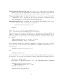
4.1.2 Creating and Handling RVS Primitives
When an object is drawn in the OpenGL scene it is displayed in the base frame by
default. To build a robot system, it is necessary to edit the position and put the object
in the right place. For this reason, some editing primitives, translation and rotation
are available:
JwEditTranslate(float x, float y, float z)
JwEditRotate(Angle angle, char axis)
These functions include the OpenGL commands to translate and rotate a created
object. In order to edit only the desired primitive, the JwEdit commands have to be
surrounded by
JwBgnEditPrimitive(JwPrimitive P)
and
JwEndEditPrimitive()
where “JwPrimitive P” represents the variable for the primitive. The following example shows how one can create and translate a cylinder using the RVS primitives library.
JwPrimitive My_Cylinder;
My_Cylinder = JwDefCylinder(24, 3.0, 3.0, JwShinyMetalMat, SeaGreen);
JwBgnEditPrimitive(My_Cylinder);
JwEditTranslate(2.5, 1.0, 3.75);
JwEndEditPrimitive();
JwDrawPrimitive(My_Cylinder);
16
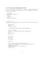
4.1.3 Creating and Handling Robot Parts
More complex objects are built from of a combination of simpler primitives. We
provide here an example that defines the motor object comprising two cylinders, a
ring and a cylinder fillet.
// Header File
typedef struct _JwMotor_ {
float r;
float len;
float h;
} *JwMotor, JwMotorRec;
// Source File
JwPrimitive JwDefMotor(float r, float len, float h, int mat, JwColor c)
{
JwPrimitive P;
JwMotor B;
float r1,r2,r3,la;
P = (JwPrimitive)JwMalloc(sizeof(JwPrimitiveRec));
P->type = JwMotorT;
P->spec = B = (JwMotor)JwMalloc(sizeof(JwMotorRec));
B->r = r;
B->len = len;
B->h = h;
r1
r2
r3
la
=
=
=
=
0.7*r;
0.6*r;
0.2*r;
1.0*r;
P->nu = 4;
P->U = (JwUnit *)JwMalloc(4*sizeof(JwUnit));
P->U[0] = def_cyl_fillet(24,r,len,(len/10),(len/10),mat,c);
JwBgnEditUnit(P->U[0]);
JwEditTranslate(0.0, 0.0,-(la+(len/2)));
JwEndEditUnit();
17
P->U[1] = def_cylinder(24,r2,(r3/6), mat,Grey|0xcc000000);
JwBgnEditUnit(P->U[1]);
JwEditTranslate(0.0, 0.0,-la+(r3/12));
JwEndEditUnit();
P->U[2] = def_ring(24,r1,r2,r3, mat,c);
JwBgnEditUnit(P->U[2]);
JwEditTranslate(0.0, 0.0,-la+(r3/2));
JwEndEditUnit();
P->U[3] = def_cylinder(24, r3,la, mat,Grey|0xcc000000);
JwBgnEditUnit(P->U[3]);
JwEditTranslate(0.0, 0.0,-(la/2));
JwEndEditUnit();
return P;
}
In the first half of the function, the memory for the primitive is reserved (JwMalloc)
and the type is specified (P->type = JwMotorT;). Furthermore all the necessary geometric parameters for the simpler primitives are calculated. The second half contains
the definition of these primitives, which are defined as four units (P->U[]) of the motor
primitive. All the required vertices for the OpenGL commands as well as the OpenGL
commands themselves will be specified within the functions for the simpler primitive.
When the JwDraw function is called for the JwMotor primitive the four objects will be
rendered on screen.
4.1.4 Deleting an Object
During the definition process, memory space for the different variables and structures is
reserved. To free this memory space again, for example when a new robot architecture
is selected, the
JwFreePrimitive(JwPrimitive P)
function is called.
4.2 Porting the RVS Primitives Library
Porting the primitives from IrisGL to OpenGL was one of the main changes required
during the programming. However, the question can be asked “Why write or port RVS
primitives when toolkits like GLUT or GLU offer routines to create 3D-objects?”. The
18
answer to this simple. All the existing robot models use RVS primitives. As a result,
all these files have to be rewritten when other routines are used.
The porting task itself can be described as a simple change of commands. Although
this task may seem to be straight forward, it is a bit tricky in the end. Often the
OpenGL Porting Guide [2] can be used to find the new command for an old one. This
is sometimes not so easy. Following three types of porting scenarios were faced.
Exact Equivalent
For some statements, the only difference is the notation. For example,
linewidth()
is the IrisGL call to change the width of a line. In the OpenGL it is:
glLineWidth()
In this case no further modifications are required.
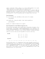
Exact Equivalent but with Different Argument List
We provide here an example of the porting scenario at hand and a description of how
it was handled. The OpenGL command glMultMatrix() is the equivalent to the
IrisGL command multmatrix(). Both commands multiply the projection matrix by
an arbitrary matrix. The difference is the way this is managed. In IrisGL the matrix
values are saved in a 4x4 array and in OpenGL it is saved in a 1x16 array.
IrisGL


a1 a2 a3 a4
 a5 a6 a7 a8 


 a9 a10 a11 a12 
a13 a14 a15 a16
OpenGL
£
¤
a1 a5 a9 a13 a2 a6 a10 a14 a3 a7 a11 a14 a4 a8 a12 a16
In general this would not be a significant problem because OpenGL reads the projection matrix in the correct order. However, one of the RVS primitives library’s handling
function JwEditMultMatrix(Matrix M) receives a matrix M of type 4x4 array. This
poses compatibility problems. To solve this problem, the matrix entries must be
placed in the correct format in a 1x16 array, before glMultMatrix() is called. This
is managed by two for-loops as follows:
19
GL_Matrix Mgl;
for(i=0;i<4;i++)
{
for(j=0;j<4;j++)
{
Mgl [i*4+j] = M[j][i];
}
}
With this solution, all the pre-defined matrices can remain unchanged in the program.
If the entries are in the wrong format the robot model is not rendered correctly; the
result being misplaced parts in the OpenGL Scene.
No Exact Equivalent
This paragraph provides an example and the solution for the type of porting scenario
without an exact equivalent. The IrisGL command cpack is used to change the active
RGBA (red, green, blue, alpha) values. It expects a single integer value in hexadecimal
notation, where the four components range from 0 to 255. For example,
cpack(0xFF004080);
sets alpha to 0xFF (255), blue to 0x00 (0), green to 0x40 (64) and red to 0x80 (128).
In RVS primitives library all the available color values are defined in “colors.h” and use
definition names like Black, SeaGreen or WarmGrey. Unfortunately, OpenGL offers no
command to set the color with a single value. As shown in the example in subsection
3.5, the color is set by three single values for the RGB mode. When the RGBA mode
is used, the command changes to glColor4f(). There are two possible ways to make
the pre-defined color values compatible with the new OpenGL command. The first
possibility would be to rewrite the header file and separate all values into four new
one. This involves rewriting all the primitives. The second option was to add two
small functions to the program which take the hexadecimal value, save the RGBA
entries in four new variables and then change the color with glColor4f(). One of
these functions is as followed:
void JwSetColor(long JwColor)
{
float nJwR, nJwG, nJwB, nJwA;
nJwR=((JwColor&0x000000ff)>>2)/255.0;
nJwG=((JwColor&0x0000ff00)>>10)/255.0;
nJwB=((JwColor&0x00ff0000)>>18)/255.0;
nJwA=((JwColor&0xff000000)>>24)/255.0;
glColor4f(nJwR,nJwG,nJwB,nJwA);
20
}
The bitwise and-operator is used to separate color value. All values are divided by
255.0 because OpenGL expects values between 0.0 and 1.0 for each settings.
21
5 Kinematics Engine
5.1 Forward and Inverse Kinematics
With the new interface and the working primitives, RVS is ready to create robot
architectures and render them in 3D. However, the program also offers animation of
robots. To accomplish this, a kinematics engine is required to solve the inverse and
direct displacement problem.
Direct Displacement Problem It may be defined as: Given the joint displacements
of a serial robot, compute the position and orientation of each link of the robot.
Inverse Displacement Problem It may be defined as: Given the EE pose (position
and orientation), find all the joint displacements of the serial robot. This problem
accepts either unique, multiple or no solution.
For both problems, a algorithm is available in the original RVS software. The engine
in hand uses only C language calls and has no elements of either OpenGL or XForms.
Hence, this source code could be implemented in the new software without any change.
5.2 Animations in FLTK/OpenGL
Calculating the new link position in Cartesian space is only half the task. The remaining half is to display the animation in the OpenGL scene. It is quite easy to calculate
the new position for each link and redraw the completed model. The effect is that
the robot “jumps” from the old posture to the new one. In fact, this is the basic
idea of motion in RVS. When the robot follows a predefined trajectory, RVS simply
renders the intermediate postures sequentially. As long as these intermediate postures
are close together, this appears to be a smooth movement. Three steps are required
to generate an animation:
1. Load the new posture from a saved file;
2. calculate the new position for each link; and
3. update the robot model.
22
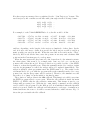
How these steps are managed is now explained for the “Joint Trajectory” feature. The
saved trajectory file contains several lines with joint angles in the following format:
θ1 (1) θ2 (1) θ3 (1)
θ1 (2) θ2 (2) θ3 (2)
θ1 (3) θ2 (3) θ3 (3)
..
..
..
.
.
.
...
...
...
...
For example, for the 7-link REDIESTRO robot, the file would look like
−101.7014
−101.6753
−101.6438
−101.6070
..
.
−17.6766
−17.6985
−17.7185
−17.7365
..
.
98.9590
98.8462
98.7321
98.6165
..
.
88.8606
88.9656
89.0719
89.1794
..
.
−25.0257
−25.2299
−25.4328
−25.6346
..
.
119.4901
119.6729
119.8611
120.0545
..
.
−113.3444
−113.5423
−113.7414
−113.9415
..
.
and has, depending on the length of the trajectory, hundreds of these lines. In the
end, it is up to the user to define how precise the whole trajectory will be and how
many postures are saved in the file. When the saved file is chosen from the “JTraj”
directory, RVS reads all the lines, saves the posture in an array and calculates link
positions in the Cartesian space for each posture.
When the user presses the play button for the forward mode, the animation starts.
At a first glance, this seems to be a simple task. Just one for-loop to set the new
postures and redraw the model. However, this is not possible because of the FLTK
routine to redraw the OpenGL scene. When the redraw() method for a widget, in this
case the Fl_Gl_Window, is called, the widget will not be updated immediately. The
widget is updated, when programm enters the FLTK main loop. The result for the
aforementioned for-loop is that the program will set the redraw() method for every
posture but only the last posture will be rendered. Therefore, the simulation would
show the robot “jump” from the initial to the final posture.
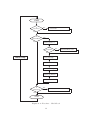
The solution to this problem is the idle callback. This function is called every time
the FLTK program waits for a new event. When the idle callback is inside the main
FLTK loop, FLTK calls the idle callback continuously. This feature is used to get
background processing done. With the Fl::add_idle() command, an idle callback
can be added to the program. For the RVS project, it is initialized when the OpenGL
window is created. Inside the callback an if-statement for each type of animation is
defined and hence the source code will be executed when the condition is true. Fig. 5.1
shows the process inside the idle callback.
23
START
if
statement 1
true
Souce Code 1
false
JT
Forward Mode
false
true
posture = posture + 1
last posture
true
false
Main Loop
Update: Joint angle
Update: Obstacle Position
Update: Slider Widget
Update: Fl_Gl_Window
Wait 0.02 sec
if
statement X
true
Souce Code X
false
STOP
Figure 5.1: Flowchart : IdleCallback
24
JT Forward Mode = false
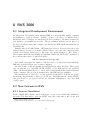
6 RVS 2006
6.1 Integrated Development Environment
An integrated development environment (IDE) is a program that assists computer
programmers to develop software. Usually, a source code editor, a compiler and/or
interpreter and a debugger are integrated in those packages. All these features are
very useful to programm big projects. The programmer includes several files to a
project, sets all the linker and compiler options and the IDE builds automatically an
executable file.
Initially, Microsoft Visual Studio .NET 2003 was selected. However, this choice was
changed latter to Dev-C++ from Bloodshed Software. Of course the company’s name
sounds a bit curious, but Dev-C++ has some very useful features to offer. First of
all it is quite small (around 10MB) and published under the GNU GPL1 , making it a
free software that can be downloaded under:
www.bloodshed.net/devcpp.html
As a result, every user who wants to edit the source code later can easily install the
IDE and open the RVS project on their computer.
Another feature of this programm are small packages called DevPaks. These packages are plug-ins (e.g. OpenGL, FLTK, GLUT) for the IDE and are also available
online. On users demand Dev-C++ can download and install all the required libraries
on the computer. The process is transparent to the IDE user/programmer.
The current version of Dev-C++ is only available for the Microsoft Windows operating system. An alternative could be Code::Blocks. This IDE runs also under LINUX,
can open Dev-C++ projects as well as use DevPaks. Furthermore, any other IDE
could be used.
6.2 New Features in RVS
6.2.1 Feature: New Robot
In the original RVS software was no function to create a new architecture within the
program. The user had to open an ASCII2 text editor and write a file for the new
1
2
GNU General Public License
ASCII American Standard Code for Information Interchange
25
(a)
(b)
Figure 6.1: Interface windows for “New Robot”: (a) Menu: Load Robot; (b) Menu: Create
Robot - Paramertes
architecture. In order to make RVS more user friendly, the program can now take care
of this task within the user interface. In this vein the user must define the number of
links (Fig. 6.1(a)), the file name, the DH parameters and the joint type (Fig. 6.1(b)).
By clicking the “save” button the program creates a new architecture file in the “Arch”
directory. The program verifies whether the selected filename already exist. In that
case the user has the choice to overwrite the existing filename or to provide another
filename. Once the new file is created it can be selected from the file browser.
6.2.2 Feature: Edit Robot
Another feature added is the ability to edit the saved parameters within the interface.
When the user changes a DH parameter, the robot is redrawn immediately in the
OpenGL scene. After all the modifications have been made, the new architecture can
be saved. Furthermore, the save option is deactivated when a fully rendered model
for the selected robot is available. For a fully rendered model, a mere change of the
DH parameters would make the full rendering incompatible. Full-renderings should
be edited as discussed in Section 6.3.
26
6.2.3 Feature: Work Environment
Generally, every robot is designed for a special family of task, e.g. pick-and-place
operations. Furthermore, the robot should work in a special work environment. To
simulate this, RVS offers a variety of objects to create a work environment. The
available list of objects is as follows:
• Table,
• conveyor,
• pallet,
• battery,
• peg,
• surface and
• fuselage.
This list could be extended in the future. Figure 6.2 shows a pick and place work
environment built around a PUMA robot. In the following two ways are discussed to
create a work environment for RVS.
Creating a Work Environment at Source Code Level
The programming of these object is similar to that of a link of a fully rendered robot
model. Every object is built from a number of primitives and defined as a new drawing
object of the type Thing. In the source code, a workspace object is than created
like a JwPrimitive object. A new variable of type Thing is declared, the geometric
parameters and the color are defined, and finally the object is rendered. The following
example shows how to create a conveyor.
Thing conveyor;
conveyor = DefConveyor(4, 2, 3, SeaGreen);
DrawThing(conveyor);
Two editing primitives are available to translate or to rotate the created object. After
each object has been defined in the source code, the whole project needs to be recompiled. This approach becomes tedious for the case when only one position parameter
for an object has to be changed. Finally, it is not possible to exchange a created work
area easily between two computers, as it is possible for architecture files.
27
Figure 6.2: Puma robot: Pick and place operation
28
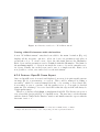
Figure 6.3: Interface window for “Work Environment”
Creating a Work Environment within the Interface
A new “Work Environment” entry has been added to the menu. A window (Fig. 6.3)
displays all the necessary options to select an object, set parameters and place it
around the robot. To create a new object, the user must increase the ID-number.
Each object and its parameters can be identified with this ID-number. The limit for
the maximum number of objects is set inside the source code and is currently set to
20 objects. Finally, the created scene can be save to a simple text file. Hence, it is
now possible to create, save and reload a work environment.
6.2.4 Feature: OpenGL Scene Export
Once an OpenGL scene is created and displayed on screen, it is quite useful generate
an image file for a presentation or a report. This could be managed by taking a
screenshot3 , which is a raster/bitmap-based file or by creating a vector-based file.
A screenshot is easy to generate, but the quality is not good enough for detailed
printouts. The advantage of a vector-based file is that the exported file will always be
a high quality image.
Therefore, a library called gl2ps, is implemented in RVS. The library can create a
vector-based file (ps,eps,pdf,svg) of a OpenGL scene. The user has to set the filename
and the desired format in the interface window and finally start the export with the
shortcut4 “crtl + e”.
3
4
Outputting the entire screen in a common format such as BMP, PNG, or JPEG
A keyboard shortcut is a key or set of keys that performs a predefined function
29
Figure 6.4: OpenGL Scene Export
Figure 6.5: Skeleton drawing of a 2-link robot
6.3 How to Create a Fully Rendered Robot
This section describes all the necessary steps to create a full rendered robot. However
first, it is important to understand how a robot skeleton is displayed on the screen. The
skeleton mode is the default mode when a fully rendered robot model is not available.
The program reads the DH parameters for the selected robot from the architecture
file and creates the links accordingly. A skeleton revolute link is L-shaped and is built
with two cylinders and one elbow primitives. For a straight prismatic link, a prism
primitive is used. Finally, the base and the end-effector drawings are always the same
for a skeleton model (Fig. 6.5).
A little more effort is required to generate the fully rendered model. Four steps are
required, to achieve the task at hand:
30
(a)
(b)
Figure 6.6: Model views of REDIESTRO: (a) Fully rendered model; (b) skeleton model
31
1. Architecture File – Every model starts with its architecture file, which could
be generated using an ASCII text editor or the newly implemented function in
the program. Appendix A shows the complete architecture file for “PUMA560”.
2. Robot File – Creating this C-language file, is the main task to obtain for a fully
rendered model. It is a file with the same name as its corresponding architecture
file. Each link is built using several RVS primitives. Further, the base and the
end-effector have to be designed with the RVS primitives. The result is a file
with several combinations of drawing and editing functions. For example, the
first link of the “REDIESTRO” model (Fig. 6.6(a)) uses 10 RVS primitives and
42 editing functions. Figure 6.6(b) shows the skeleton model for the same robot
with the standard link design.
3. Modifications – Once the Robot file is complete, the files “Links.h” and “Links.c”
have to be modified. In these files, the new robot file must be implemented, so
that the program can render the full geometry when the architecture is selected.
The “Links.*” files include functions to draw the defined model.
4. Recompiling – The last step is to compile the new robot file and the modified
files to create a new executable file.
32
RVS 2006
include
src
rs
Arch
graphics
Ctraj
links
matrix
gl2ps
JConfig
Jtray
Workarea
Figure 6.7: RVS2006 - Directory tree
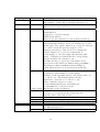
6.4 File and Folder Overview
The major problem during the analysis of the original RVS was the lack of documentation. As mentioned in Chapter 2, the RVS user manual offers little in the overview
of files and folders. This becomes particulary evident when some of the important
files are not even mentioned in the available overview. Hence, the only way to find a
functions was to go through the source code which was tedious and time consuming.
To facilitate future programmers we aim to include a more detailed overview of the
file structure. In the interest of space a general outline is provided. Figure 6.7 shows
the directory tree of the RVS project and the following explains the folders and special
files.
Directory
\include
Filename
colors.h
primitives.h
robot.h
\rs
\rs\Arch
\rs\Ctraj
\rs\Jconfig
Explanation
This directory contains the header files
for some source files.
Available color definitions
Type definition for all RVS primitives.
Structure definition for a link,
the end effector and the robot.
This directory contains the main source files.
Robot architectures are saved in this directory.
Files with the cartesian trajectories are saved in this folder.
Posture files for the different robots.
33
Directory
\rs\Jtraj
Filename
\rs\Work_Env
main.c
menu.*
opengl_win.c
opengl_win.h
reader.*
ikp.c
setting.c
RVS2006.exe
\src
axes.c
Explanation
Saved files for joint trajectories.
An example of such a file is available in Section 5.2.
The created work area scenes mentioned in
subsection 6.2.3 are saved here
Source code for the main program
main-function
declaration of global variables
FLTK main window
function gl_win_redraw() for the redraw()-method
Source code for the menu
The menu.c file includes one block of functions for each
menu entry. The “main” function (to create the window)
for each block should give the name for each
function and widget of the block. For example the
“main” function to load a new architecture is
void arch(), so all other names should start with
arch_. Callbacks are named like the corresponding
widget and have the extension _cb.
Because the file got very large some functions are
saved in new files which are named menu_filename.c
The Function Robot NewRobot(char *name) is
called when an new robot is selected from the list.
Source file for the Fl_Gl_Window
Constructor and destructor for the widget.
Settings for the OpenGL window, like background color,
colormode, etc. The draw() which calls the
functions to draw the robot, the floor, the
effector and the trajectory course.
void IdleCallback() for all animations.
void handle() for all I/O actions.
Header file for the declaration.
Header and source file for functions to
load new robot data from the architecture file
and the data for the trajectories.
Source file with the functions for the kinematic engine.
Source file for all the workspace objects.
Executable file for WIN32 applications.
This directory contains the source files
for different functions
Provides two functions to draw frames at the base,
34
Directory
Filename
light.c
primitives.c
\links
links.c
robotname.c
\matrix
\gl2ps
Explanation
each joint and the end effector.
void JwAxes_xyz(float len, JwColor color)
void JwAxes_XYZ(float len, JwColor color)
Source code for all the light settings in the
OpenGL scene. void JwInitLight()
Function JwSetColor() to change the defined color
value in single RGBA values.
Source code for all the basic primitives. (Chapter 4)
Includes files for the fully rendered models.
Functions to check for a fully rendered model.
These are the files for the defined fully rendered models.
This folder contains several files for mathematical
operations, such as cross product, matrix vector
multiplications or Cholesky decomposition.
This folder contains all files for the gl2ps library
6.5 Required Library files
To compile the source code some libraries have to be added to the linker options. The
following table includes all required libraries for a WIN32-application.
FLTK library
Libraries used by FLTK
OpenGL library for FLTK
Standard OpenGL library
GLU library
Windows GDI
35
libfltk.a
libole32.a
libuuid.a
libcomct32.a
libwsock32.a
libm.a
libfltk_gl.a
libopengl32.a
libglu32.a
libgdi32.a
7 Geometry of Serial Robots
7.1 Revolute and Prismatic Links
The architecture of a serial robot can be described as an assembly of several rigid
bodies, or links, thereby forming what is known as a kinematic chain. Two links are
coupled by a kinematic pair, also termed a joint. Depending on the type of contact
between the two links, the kinematic pair can be either lower or higher. Only the two
basic lower types are considered here, as their higher counterparts appear in robots
only exceptionally.
Turning Pair This type is also called a revolute joint. The contact surface between
the two links is a surface of revolution not allowing sliding along its axis of
symmetry. As a result, the two links can only rotate about the foregoing axis
with respect to each other.
Example: Journal bearing
Sliding Pair This pair, also called a prismatic joint, allows for a relative pure-translation
motion. This pair, contrary to the revolute, has no axis only a direction of
motion.
Example: Dovetail coupling
The kinematic chain can be also of one of two types. In a closed chain, each link is
coupled to two other links. This chain is also called a linkage. The chain is an open
chain, when it contains exactly two links that are connected to only one other link.
Hence, a serial robot is an open kinematic chain, because the first and the last link
are only connected to one other link. In robotics the first link is called the base, the
last link is the end-effector.
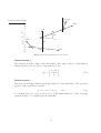
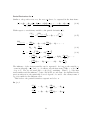
7.2 Denavit-Hartenberg Notation
For a robotic architecture each link, except the base and the end effector, lies between
two kinematic pairs. In order to describe the robot geometry precisely, the DenavitHartenberg notation (Denavit and Hartenberg, 1955) is introduced. All links are
numbered from 0 (base) to n (end-effector) and each pair is defined as the coupling
between the (i–1)st and ith link. Next, a coordinate frame Fi (Oi , Xi ,Yi , Zi ) is
defined, which is connected to the (i–1)st link. Therefore, the frames are numbered
36
from i = 1, 2, . . . , n + 1. Following the rules for the Denavit-Hartenberg notation,
illustrated in Fig. 7.1, and assuming only revolute joints,
1. Zi is the axis of the ith kinematic pair
2. Xi is the common perpendicular from Zi−1 to Zi (If these two axes are parallel,
then the location of Xi is undefined.) Yi is defined by the right-hand rule.
3. ai is the distance between Zi and Zi+1 , this is the link lengths
4. bi is the Zi -coordinate, of the intersection of Zi with Xi+1 . Parameters bi is also
called the link offset and can be positive or negative.
5. αi is the angle between Zi and Zi+1 measured positive in the direction of Xi+1 .
This parameter is called twist angle.
6. θi is the angle between Xi and Xi+1 measured positive in the direction of Zi+1 .
This angle is called the joint angle.
Because a robot does not have a (n+1)st link, these rules do not apply to the last
frame. Therefore, the frame can be defined arbitrarily, but its origin is placed at a
specific point, the operation point P, of the end-effector. In summary, the kinematic
chain contains n + 1 links, n + 1 frames and n kinematic pairs.
The three variables ai , bi and αi are called the joint parameters and represent the
fundamental geometry of the robot. The architecture of each link is defined by the set
of these parameters. They are constant because the architecture of a robot does not
change when the robot moves. What changes is the joint variable θi .
In order to describe the complete architecture and posture of a n-link robot 3n joint
parameters and n joint variables are needed. This leads to 4n Denavit-Hartenberg
parameters for the robot.
Position vectors ei
The vector ei is defined along the Z -axis of the frame Fi . In frame Fi , this vector
components are
 
0
[ei ]i ≡  0 
(7.1)
1
37
PSfrag replacements
Zi−1
Zi
θi
ai
0
O i−1
Oi
Oi+1
αi s01
Zi+1
Xi+1
Xi s05
bi
0
Oi
s08 s09
s010
s02
s07
s04
s03
s013
s012
s06
s011
Figure 7.1: Denavit-Hartenberg Notation
Position vectors ai
The directed from the origin of the ith frame to the origin of the (i + 1)st frame is
defined by the vector ai , whose components in Fi are


ai cos θi
(7.2)
[ai ]i =  ai sin θi 
bi
Position vectors ri
The vector ri is defined directed from the origin Oi of the ith frame to the operation
point P of the end-effector, namely,
ri = ai + ai+1 + ai+2 + . . . + an
(7.3)
To calculate the above vector, all vectors on the right–hand side of the foregoing
expression have to be expressed in the ith frame.
38
7.3 Rotation Matrix Qi
The matrix Qi is used to transform a vector or a matrix from the i + 1st frame into
the ith frame. This matrix is given by [10]


cos θi − cos αi sin θi sin αi sin θi
Qi =  sin θi cos αi cos θi sin αi cos θi 
(7.4)
0
sin αi
cos αi
For example, vector ri expressed in the ith frame is:
ri = ai + Qi ai+1 + Qi Qi+1 ai+2 + . . . + Qi · · · Qn−1 an
39
(7.5)
8 Tools for the Optimum Design of
Robots using Gradient Methods
8.1 Introduction
The design of a new robot starts with the determination of performance specifications
that should be achieved by the robot. On the basis of these specifications the various
links will be designed. There are different methods to define the fundamental geometry
for a robot, like Burmester Theory or the minimization of the condition number of
the Jacobian matrix at one robot posture. The latter approach was used of Khan
and Angeles[3] and is also used in this project. The following sections give a brief
introduction.
Remark
For brevity, the details of derivations below are not included in this report, but the
pertinent references are included.
8.2 Mathematical Background
8.2.1 The Jacobian Matrix
In robotics the Jacobian Matrix (J) is defined as a 6 × n matrix mapping the set of
joint rates θ̇) into the twist (t) of the end-effector, namely,
Jθ̇ = t
where
·
J=
e1
e2
···
e1 × ri e2 × r2 · · ·
en
en × rn
¸
8.2.2 Condition Number
The condition number is a measure of the roundoff error amplification of the computed
results with respect to the roundoff error of the input data. The general definition of
40
the condition number of a nonsingular matrix A is possible when all matrix entries
have the same physical units. In that case the condition number is defined as
κ(A) = kAkkA−1 k
(8.1)
where k · k stands for a arbitrary matrix norm. In this report the Frobenius norm k · kF
is used throughout. The Frobenius norm of the n × n nonsingular matrix A s defined
as
r
r
1
1
T
kAkF =
tr(AA ) =
tr(AT A)
(8.2)
n
n
The Frobenius norm of A−1 is defined as
r
r
r
1
1
1
kA−1 kF =
tr(A−1 A−T ) =
tr[(AT A)−1 ] =
tr[(AAT )−1 ]
n
n
n
Finally, the Frobenius–norm condition number of A is given by
q
q
1
1
T
T −1
κF (A) =
tr(AA )tr[(AA ) ] =
tr(AT A)tr[AT (A)−1 ]
n
n
(8.3)
(8.4)
For brevity, we shall refer to κF (A) simply as the condition number of A.
8.2.3 Concept of Homogenous Space
As long as, the Jacobian matrix contains entries with nonhomogeneous dimensions,
the condition number cannot be calculated. To solve this problem, the concepts of
homogenous space and characteristic length are introduced. The goal of this concept is to make all the entries dimensionless. The homogenous space is defined as a
dimensionless Euclidean space.
Similar to the Denavit-Hartenberg notation frames, vectors and distances can be
defined in homogenous space. With the same rules the homogenous counterparts ai ,
bi of the DH parameters ai and bi are defined. The two angles αi and θi bear no
physical units while the two variables ai and bi are nothing but length ratios, i.e.,
ai
L
bi
=
L
ai =
bi
where L is the characteristic length, as yet to be defined. With the foregoing homogenous variables, the dimensionless counterparts ai and ri of the vectors ai and ri are
41
then defined, the homogeneous Jacobian Matrix H taking the form
·
¸
e1
e2
...
en
H=
e1 × r1 e2 × r2 . . . en × rn
(8.5)
8.3 Optimization Problem
The approach, mentioned in the Introduction, optimizing the robot dimensions over
its architecture parameters and joint variables, is adopted here. For a n-axis robot,
4n design parameters are available over which the designer can minimize the condition number of the Jacobian matrix. Three of these parameters do not influence the
condition number. The remaining 4n − 3 design variables are group in a design vector
x in the form
£
¤T
x = a1 α1 a2 b2 α2 θ2 · · · an bn θn
(8.6)
In this report, we restrict ourselves to th robots with six revolute joints, which leads
to n = 6, and hence, a 6 × 6 homogeneous Jacobian matrix. The optimum design
problem is then defined as
minκF (H)
(8.7)
x
subject to the constraints
kei k = 1,
ei · ri = 0,
i = 2, . . . , n
i = 1, 2, . . . , n
(8.8)
(8.9)
The number of the first set of constraints is n − 1, that of the second set is n, which
leads to 2n − 1 constraints for a n-joint robot.
8.4 Method of Solution
In [3] the direct method was used to solve the optimum design problem. In this project,
the application of a gradient method, like the Orthogonal-Decomposition Algorithm[4]
is investigated. The problem is defined as:
f (x) → min
x
(8.10)
h(x) = 0
(8.11)
tr(HHT )tr[(HHT )−1 ]
(8.12)
subject to the constraints
where
f (x) =
1
6
q
42
Vector h includes the left-hand sides of constraints 8.8 and 8.9, namely,


ke2 k2 − 1
..


.




2
 ken k − 1 
h=

 e1 · r1 


..


.
en · ri
(8.13)
The Orthogonal-Decomposition Algorithm requires the gradient and the Hessian of
the objective function and the gradient of the vector h. For the ensuing derivations
the objective function can be simplified. For starters, this function is squared, for the
function will be minimized when its square is minimized. Moreover, the factor 1/36
can be dropped, for it has no effect on the minimum. We thus have the new objective
function
z = tr(HT H)tr[(HT H)−1 ] → min
(8.14)
x
which is factored into two functions, namley,
f1 = tr(HT H)
f2 = tr[(HT H)−1 ]
(8.15)
(8.16)
∇z = f2 ∇f1 + f1 ∇f2
(8.17)
This leads to the gradient
8.4.1 Gradient of f1
The gradient of f1 with respect to a vector x is defined as
·
¸
¤
∂ £
∂ ¡ T ¢
T
tr(H H) ≡ tr
H H
∂x
∂x
(8.18)
which thus leads to a third-rank tensor. As a means to avoid cumbersome third-rank
tensors, we express the above gradient in the form

 

tr(∂HT H/∂x1 )
∂tr(HT H)/∂x1
T
T

 
¤ 
∂ £
 ∂tr(H H)/∂x2   tr(∂H H/∂x2 ) 
T
(8.19)
tr(H H) = 

=
..
..
∂x

 

.
.
tr(∂HT H/∂xl )
∂tr(HT H)/∂xl
For each entry of the design vector x, a partial derivative of HT H with respect to a
scalar has to be calculated, which yields a matrix. Since the trace of a matrix is a
43
scalar, all array entries in eg. 8.19 are scalar. The product of the two matrices is a
square, symmetric matrix, i.e.,


eT1 e1 + (e1 × r1 )T (e1 × r1 ) · · · eT1 e6 + (e1 × r1 )T (e6 × r6 )


..
..
..
HT H = 
 (8.20)
.
.
.
e6 eT1 + (e6 × r6 )(e1 × r1 )T · · ·
eT6 e6 + (e6 × r6 )T (e6 × r6 )
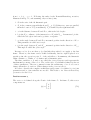
whose entries are all dimensionless, whence,
¡
¢
tr HT H = ke1 k2 + ke1 × r1 k2 + · · · + ke6 k2 + ke6 × r6 k2
(8.21)
Because the 2-norm of the unit vector ei is 1 its derivative with respect to any variable
vanishes. The second derivatives of terms k(ei × ri )k2 with respect to xj are calculated
as
¤
∂kei × ri k2
∂ £
=
(ei × ri )T (ei × ri )
∂xj
∂xj
·
·
¸T
¸
∂(ei × ri )
T ∂(ei × ri )
=
(ei × ri ) + (ei × ri )
∂xj
∂xj
µ
¶T
∂(ei × ri )
= 2
ei × ri
∂xj
µ
µ
¶
¶
∂ei
∂ri
∂(ei × ri )
=
× ri + ei ×
∂xj
∂xj
∂xj
(8.22)
(8.23)
(8.24)
(8.25)
In order to compute the gradient of the objective function, the partial derivatives of
vectors ei and ri with respect to vector x have to be computed.
Partial Derivatives for ei
The vector ei has to be expressed in the first frame F1 . In the ith frame the vector is
always ei = [ 0, 0, 1 ]T , which leads to
 
0

[ei ]1 = Q1 Q2 . . . Qi−1 0 
(8.26)
1
44
The derivative of ei with respect to an arbitrary variable y representing any of the
design parameters thus becomes
¢
∂ [ei ]1
∂ ¡
=
Q1 Q2 . . . Qi−1 ei
∂y
∂y
∂Q2
∂Q1
=
Q2 . . . Qi−1 ei + Q1
Q . . . Qi−1 ei + . . . +
∂y
∂y 3
∂ei
Q1 . . . Qi−1
∂y
(8.27)
(8.28)
This formula can be simplified for the given design variable. It is obvious that any
derivative of the vector ei (≡ [ei ]i ) is zero. Furthermore the matrices Qi do not depend
on the variables a and b, which leads to:
∂Qi
= 0
∂ai
∂Qi
= 0
∂bi
∂ei
= 0
∂y
(8.29)
(8.30)
(8.31)
The transformation matrices reach from the first to the (i − 1)st frame. Therefore, the
design variables α and θ for the ith frame or any following frame have also no influence
on the partial derivative of ei . The partial derivatives reduce to the two expressions
below
∂Qj
∂ [ei ]1
= Q1 . . . Qj−1
Q . . . Qi−1 ei
∂αj
∂αj j+1
∂Qj
∂ [ei ]1
= Q1 . . . Qj−1
Q . . . Qi−1 ei
∂θj
∂θj j+1
Where the derivatives for the matrix Q are defined as:


0
sin
α
sin
θ
cos
α
sin
θ
j
j
j
j
∂Qj
=  0 − sin αj cos θj − cos αj cos θj 
∂αj
0
cos αj
− sin αj


cos
θ
−
cos
α
sin
θ
sin
α
sin
θ
j
j
j
j
j
∂Qj
=  sin θj cos αj cos θj − sin αj cos θj 
∂θj
0
sin αj
cos αj
45
(8.32)
(8.33)
(8.34)
(8.35)
Partial Derivatives for ri
Similar to the position vector ei , the vector ri has to be expressed in the first frame:
[ri ]1 ≡ Q1 . . . Qi−1 (ai + Qi ai+1 + Qi Qi+1 ai+2 + . . . + Qi . . . Qn−1 an )
| {z } |
{z
}
Q1...(i−1)
r
=
r
[ i ]i i
With respect to an arbitrary variable y the partial derivative [ri ]1 ,
µ ¶
¶
µ
∂Q1...(i−1)
∂ [ri ]1
ri
ri + Q1...(i−1)
=
∂y
∂y
∂y
(8.36)
(8.37)
∂Q1...(i−1)
∂Q1
∂Q2
=
Q2 . . . Qi−1 + Q1
Q . . . Qi−1 + . . . +
∂y
∂y
∂y 3
Q
Q1 . . . Qi−2 i−1
(8.38)
∂y
µ
¶
ri
∂Qi
∂ai
∂ai+1
=
+
ai+1 + Qi
(8.39)
∂y
∂y
∂y
∂y
µ
¶
∂Qi+1
∂Qi
∂ai+2
+
Q ai+2 + Qi
ai+2 + Qi Qi+1
+ ... +
∂y i+1
∂y
∂y
µ
¶
∂Qi
an
+
Q . . . Qn−1 an + . . . + Qi . . . Qn−1
∂y i+1
∂y
The influence of the design variables can be separated. As long
£¡ as the variable¢ x¤j
occurs in either Qj or aj , and j < i, it affects only the first term ∂Q1...(i−1) /∂xj ri
£
¤
of eq. 8.37. The second term Q1...(i−1) (ri /∂xj ) vanishing. When j ≥ i the first
term vanishes and the influence occurs only in the second term. As explained in the
previous subsection, the matrix Q does not depend of a and b. Also many terms of
eq. 8.39 vanish for the different cases.
This leads to the partial-derivatives expressions below: r:
for j < i
∂Qj
∂ [ri ]1
= Q1 . . . Qj−1
Q . . . Qi−1 ri
∂αj
∂αj j+1
∂Qj
∂ [ri ]1
= Q1 . . . Qj−1
Q . . . Qi−1 ri
∂θj
∂θj j+1
46
for j = i
∂ [ri ]1
∂aj
∂ [ri ]1
∂bj
∂ [ri ]1
∂θj
∂ [ri ]1
∂αj
µ
=
=
=
=
¶
∂rj
Q1...(i−1) Qi . . . Qj−1
∂aj
µ
¶
∂rj
Q1...(i−1) Qi . . . Qj−1
∂bj
¶
µ
∂Qi
∂ai ∂Qi
ai+1 + . . . +
Q1...(i−1)
+
Q . . . Qn a n
∂θj
∂θj
∂θj i+1
µ
¶
∂Qi
∂Qi
Q1...(i−1)
Q . . . Qn a n
ai+1 + . . . +
∂αj
∂θj i+1
for j > i
µ
¶
∂ [ri ]1
∂aj
= Q1...(i−1) Qi . . . Qj−1
∂aj
∂aj
µ
¶
∂ [ri ]1
∂aj
= Q1...(i−1) Qi . . . Qj−1
∂bj
∂bj
∂Qj
∂ [ri ]1
∂aj
= Qi . . . Qj−1
+ Qi . . . Qj−1
aj+1 + . . . +
∂θj
∂θj
∂θj
∂Qj
Q . . . Qn−1 an
Qi . . . Qj−1
∂θj j+1
∂Qj
∂Qj
∂ [ri ]1
aj+1 + . . . + Qi . . . Qj−1
= Qi . . . Qj−1
Q . . . Qn−1 an
∂αj
∂αj
∂αj j+1
8.4.2 Gradient of f2
In functions f2 , the inverse of the matrix product comes into the picture, and hnece,
the gradient of an inverse matrix A−1 is needed. This is readily calculated below:
From we obtain, upon differentiation with respect to y, whence,
AA−1 = 1
µ
¶
µ
¶
¢
∂ ¡
∂A
∂A−1
−1
−1
AA
=
A +A
=O
∂y
∂y
∂y
µ
¶
∂A−1
∂A
−1
= −A
⇒
A−1
∂y
∂y
47
(8.40)
The gradient of f2 thus reduces to
·
¸
·
¸
¡ T ¢−1 ¡ T ¢−1 ∂(HT H)
∂(HT H)−1
tr
= −tr H H
H H
∂y
∂y
"
¡ T ¢#
h¡
i
¢2 −1 ∂ H H
= −tr
HT H
∂y
(8.41)
(8.42)
All derivatives required in the above expression were defined in the previous subsections.
8.5 Conclusion and Recommendations for Further
Work
During this project, only a first attempt to compute the gradient of the objective function was programmed. Because the final algorithm should be available in a MATLAB
and implemented in RVS, MATLAB was used for the first developments. In order
to minimize the changes between the MATLAB and the C codes, only methods are
used that are basic C functions or available in the RVS mathematical library. The
RVS mathematical library (matrix - folder) includes several function to calculate, for
example, a cross product, matrix × vector multiplications or the Cholesky decomposition. Also, a function to compute the Jacobian matrix is implemented in RVS.
However, as long as C does not support symbolic calculations every partial derivative
has to be programmed. This could be managed in two ways:
1. The algorithm builds the partial derivative for each combination of ei or ri and
the design variables. This requires several if and switch statements for each
equation, but the final calculations are minimized. (This method was used in
the first attempt for the gradient calculation.)
2. Another possibility is to calculate first the partial derivative of matrices Qi and
vectors ai with respect to each design variable and use the general expressions for
∂ [ei ]1 /∂x and ∂ [ri ]1 /∂x. In this case the number of if and switch statements
would be less, but the number of calculations higher.
Implementation in RVS
Although the development of the algorithm is not very advanced at this stage, we
suggest a list of the planned steps for RVS implementation:
1. Use the pre-saved DH-parameters as the initial guess
2. Show a rendering of the new architecture after each interaction
48
3. Create a new architecture file or overwrite the existing file. The overwrite function should be deactivated, when a fully rendered model is defined for the select
architecture.
49
9 Conclusion and Recommendations
for Further Work
Conclusion
The Robot Visualization System 2006 (RVS2006) is a free software package for the
simulation of robots (Appendix B). With the program it is possible to render a skeleton
model or a fully rendered model of a robotic architecture. For a skeleton model only
an ASCII-file with the DH parameters is required. The fully rendered model has to
be programmed for each robot individually.
In order to make RVS2006 operating system independent only cross-platform software packages are used. The program is written in C/C++ and OpenGL is used for
all 3D renderings. In combination with the Fast and Light Toolkit, RVS2006 is available for Microsoft Windows, LINUX and MacOS. All main features from the original
RVS are implemented in RVS2006. Some functions, e.g. reading data from an external floppy disk, are no longer required for the software. Therefore, these parts have
not been implemented in RVS2006. The following list includes all features that are
available in RVS2006:
• Create / load a new robot;
• edit an existing architecture;
• select rendering mode for a robot;
• choose different end-effectors;
• display frames;
• set joint limits;
• load saved postures;
• control each joint variable individual;
• cartesian configuration;
• trajectories on basis of joint variables;
50
• place obstacles;
• select different payloads;
• create a work environment; and
• export OpenGL scene.
Recommendations for Further Work
Although most of the functions work properly the source code still contains some bugs
which could not be fixed during this project. This has to be done in the future. A
list of known bugs is provided in Appendix C. In the original RVS the Cartesian
Trajectory feature was mentioned. However, this function was not working in RVS
and it is still not working in RVS2006. Only an interface for this feature has been
created and some old functions were implemented. Currently the menu entry for this
function is not shown.
51
Bibliography
[1] Wu, C.J., Angeles, J., and Montagnier, P., 1997, Robot Visualization System (RVS)
User Manual, Centre for Intelligent Machines (CIM) Department of Mechanical
Engineering McGill University, Montréal, Québec, Canada
[2] Fryer, B., Hartman, and J., Silverio, C.J., 1997, OpenGLrPorting Guide, Silicon
Graphics, Inc.
[3] Angeles, J., and Khan, W., 2006, The Kinetostatic Optimization of Robotic Manipulators: The Inverse and the Direct Problem, Journal of Mechanical Design
[4] Angeles, J., 2006, MECH 577 Optimum Design - Lecture Notes, Centre for Intelligent Machines (CIM) Department of Mechanical Engineering McGill University,
Montréal, Québec, Canada
[5] van der Zijp, J., 2005, FOX Toolkit Documentation, http://fox-toolkit.org
[6] Kilgard, M.J., 1996, The OpenGL Utility Toolkit (GLUT) Programming Interface,
Silicon Graphics, Inc.
[7] Rademacher, P., 1999, GLUI - A GLUT-Based User Interface Library,
http://glui.sourceforge.net/
[8] Earls, C.P., Spitzak, B., and Sweet, M., 2006, FLTK 1.1.7 Programming Manual,
http://www.fltk.org
[9] Angel, E., 2002, OpenGL - A Primer, Addison-Wesley
[10] Angeles, J., 2006, Fundamentals Of Robotic Mechanical Systems, 3rd ed, SpringerVerlag, New York
52
Appendix A
Architecture File: REDIESTRO
/*************************
REDIESTRO
*************************/
geomtype = full
/** Link 1 **/ {
a = 0.0
b = 9.5229
al = -58.3127
th = 0.0
limits = [ -170.0, +95.0 ]
}
/** Link 2 **/
{
a = 2.311300
b = -0.2291
al = -20.0289
th = 20.0
/** limits = [ -210.0, +45.0 ] **/
}
/** Link 3 **/
{
a = 0
b = 0.369275
al = 105.2568
th = 40.0
/** limits = [ -45.0, +185.0] **/
}
/** Link 4 **/
{
53
a = 3.9884
b = 0
al = 60.9094
th = 20.0
/** limits = [ -35.0,
+180.0] **/
}
/** Link 5 **/
{
a = 0
b = -4.71588
al = 59.8823
th = 40.0
}
/** Link 6 **/
{
a = 1.35589
b = 5.78206
al =-75.4715
th = 10.0
}
/** Link 7 **/
{
a = 1.7835 /* 2.3445 */
b = -1.4505
al = 0
th = 210.0
}
EndEffector = hand
54
Appendix B
RVS2006 Screenshot
55
Figure B.1: RVS2006
56
Appendix C
Bugs in RVS
• Fully rendered model of TravPuma
• Missing labels on frame axes
57