Download physics auxiliary publication service - AIP FTP Server

PHYSICS AUXILIARY
PUBLICATION SERVICE
Document No:
PFLDA-29-1558-22
Journal Reference:
PHYSICS OF FLUIDS
Title:
Authors:
User's Manual for the Flora Equilibrium
& Stability Code
B.1. Cohen & R.P. Freis
Current Physics Microform Reference:
8605C
0001
A service of the American Institute of Physics
UCID.20400
User's Manual for the FLORA Equilibrium
and Stability Code
Robert P. Freis
Bruce I. Cohen
A p r i l 1, 1985
April
T h i s is an informal rejort intended primarily for internal or limited external distribution. The
opinions and condusions stated are those o f the author and may or niay not be those o f the
Laboratory.
W o r k performed under the auspices o f the U . S . Department o f Energy by the Lawrence
Livermore Laboratory under Contract \V-7405-Kng-48.
'DISCLAIMER
This document was prepared as an account of work sponsored by an agency of Ihe United Slal&Government.
Neilher Ih~ United States Governmenl nor t~ Universily of california nor any of their employees, mak"" any
warranty. express or'implied. or assumes any leRal Iiabilily or responsibilily for the accuracy. completeness, or
usefulness of any informalion. apparalus, producl, or process disclosed. or represents Ihal its use would nol infringe
privately owned righls. Reference berein 10 any specific commercial p~odUds, prCKeSS, or senice hy Irade name.
trademark, manufaclurer. or otherwise. does not necessarily constitute or imply its endorsement, recommendation, or
favoring by the United Slales Governmenl or the University of California. 'The views and opinions of authors
. expressed here,in do not necessarily slate or reOed tbose of Ihe United Slales Government or tbe University of _
California, and shall not be used for advertising or product endorsement purposes.'
Prtnted in the United Stiles ot Amrrin
Av.iI~blt from
N.tion.al Techntca! Inform.ltion Servic~
U.5. Department of Commerce
5285 Port Roy,1 R,,'d
Spdngfirld. V~ 22161
Price: Printed Copy S
; Microfiche- 54.50
Page Range
001-025
026·050
051-075
076·100
101-125
126-150
151-175
"l76-200
201-225
226-250
251-275
276-300
301-325
Domestic
Price
S 7.00
8.50
10.00
11.50
'13.00
14.50
16.00
.17.50
19.00
20.50
22.00
23.50
25.00
Page Range
326-350
351-375
376-400
401-426
427-450
451-475
476-500
501-525
526-550
551-575
576-600
601- u p l
Domestic
Price
$
26.50
28.00
zs.sn
3i.00
32.50
34.00
35.50
37.00
38.50
40.00
41.50
Add 1.50 for each additional 25 page increment, or port ibn
thereof from 601 pages u~.
User's Manual For The FLORA Equilibrium And Stability Code
Robert P. Freis and Bruce 1. Cohen
Lawrence Livermore National Laboratory
Livermore, Ca. 94550 USA
Abstract
This document provides a user's .guide to the content and use of the two-dimensional
axisymmetric equilibrium and stability code FLORA. FLORA addresses the low-frequency
MHD stability of long-thin axisymmetric tandem mirror systems with finite pressure and
finite-larrnor-radius effects. FLORA solves an initial-value problem for interchange, rotational, and ballooning stability,
1
INTRODUCTION
This user guide is a brief description of the FLORA code and is designed to be used in
conjunction with the code lisitng. The theory and general equations which this -program
solves are described elsewhere 1., 2 in detail.
FLORA solves, in a 2-D domain (z,'l/J), for the linearized stability of a:. long thin axisymmetric equilibrium. It uses an initial-value method in which .an equilibrium is given an
initial perturbation to its magnetic B field, and the time behavior of the perturbation is
followed. The perturbation has been Fourier expanded in the azimuthal (fJ) direction and
each mode (m) must be examined separately. The values of m can be arbitrary with an
upper limit around 0(103 ) because of accuracy consideration as the modes become more
highly localized.
The complex partial differential equation of motion for the perturbed radial displacement
of the field lines (Appendix A). is solved as a coupled .system of two real p.d.e.'s and the
solution consists of two parts, the real part (called X RO in FLORA) and the imaginary
part (called XIO ). The system is solved by bringing the coupling terms in each equation
to the right hand side and using an iterative technique.
2
FLORA EQUILIBRIUM OVERVIEW
FLORA equilbrium are specified by the following spatial quantities:
pressure (P.l.,P II)
density
vacuum B fields
electric potential </J
Tandem mirror systems are simulated by assuming symmetry around the midplane (z = Q)
and calculating half of the total system. The half system can consist of either two or
three cells, referred to as the center cell, the choke cell, and the end-plug cell. The cell
boundaries are defined by solenoids which generate the vacuum B fields. Within each cell
several pressure components (both. perpendicular and parallel) can be specified which will
satisfy pressure balance equations and, together with the vacuum B fields, will generate the
self-consistent finite- j3 B fields. Densities and potentials are defined by analytic' functions
(Appendix A). The potentials are not self-consistent with the equilibria.
1
3
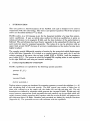
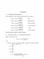
VACUUM B FIELDS
The vacuum B at any point in space is
NeOIL.
L
BV AC(z) =
bS(ZSCl
z)
+ BCENTER(z)
8=1
(independent of'l/J because ofthe paraxial model) Ncoil is.2 or 3. b, is th on-axis B; field of
a solenoid located at ZSC (Appendix A). BCENTER is a constant from z :- 0 to a specified
transition region (z = ztrans) beyond which it rapidly falls away (see Appendix A). It is
designed to represent the center cell vacuum magnetic field.
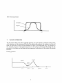
For a 3-region case (NCOIL.= 3)
Bmex
Bvx2
\
center
choke
eel J
cell
Bvx3
\
end plug
cell
-,
Bm'nl
Bmn2
zlc
z2c
For a 2-region case (NCOIL = 2)
Bmex
end plug
center
cell
cell
8mnl
zlc
z t rrn n
z2c zrnax
2
22ml n
z3c
Note:
1. BMAX, BVX2, BVX3, BVa are the resultant values due to all the sources present.
2. Each solenoid is specified by 4 input parameters:
B field strength (Gauss)
axial length (cm)
radius (cm)
ζ location of center (cm)
(zic,Z2c,Z3c)
~he magnetic field strength input is actually the desired total vacuum magnetic field at
the center of each solenoid on axis, excluding the center cell field .
4.
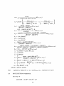
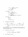
PRESSURE
The general form of the perpendicular pressure is
s
where p .Le is due to hot electrons and the sum is over all other species. This is solved
together with the perpendicular pressure balance equation,
Then the parallel pressure is obtained from the parallel pressure balance equation,
Pi. = -B
2
d (PII / B )
dB
or
PII(~p,B) = LP~s('lj;)
(-1- B 4 - bs B
2
+ Cs + ds B)
e
The coefficients as, b, c , and d , are calculated from the conditions for zero pressure and
zero slope at appropriate axial positions.
In addition, in the center cell there can be a z-independent pressure component (ppas 1)
with Pl. = PI\ = coristant with respect to B. In the 'outer cells the passing component has
B dependence.
The passing and trapped groups will be described separately, following a brief description
of the hot-electron pressure.
3
5.
HOT ELECTRON PRESSURE
The perpendicular hot electron pressure,
is separated from the other species in order to properly treat it as a" stiff" component in the
manner of the rigid Elmo Bumpy Torus model 3 ,4 . It is included in the total perpendicular
pressure only when calculating the magnetic B fields. It is not included in other pressuredependent' equilibrium quantities, for example Q(= B 2 + P.l. - PH)' It is therefore not
dynamically included as a source of instability. In addition, the hot-electron density is
assumed to be negligible, compared to the warm electron and ion densities, in order to
satisfy charge neutrality. Note that this does not imply a constraint on the hot electron
pressure.
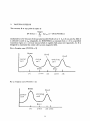
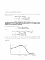
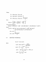
6.
TRAPPED PRESSURE
Each cell can contain a trapped species whose P.l. peaks at the B field minimum and goes
to zero with zero slope at the cell limits. In the case of unequal magnetic mirror peaks
the smaller magnetic field peak determines the maximum magnetic field beyond which the
pressure is zero. In the plug cell a sloshing profile is constructed from the difference of
two trapped profiles. A hot electron pressure can exist in the cell adjoining the central
cell(i.e. the choke cell in the three region case, the end plug cell in the two region case).
A code option permits the axial profile of the hot electrons to be elongated with a region
of constant pressure.
3 region case
psloah
peen
z3c
z2e
zlc
pslosh
peen
2 region case
z2c
zle
4
Hot electron pressure
elonceteo
r ecular __
23
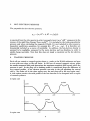
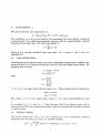
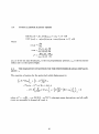
7.
PASSING PRESSURE
For the three region case only, a passing pressure can exist which is constant in the center
cell, minimizes at the minimum B field of the choke cell, peaks at the entrance to the end
plug cell and goes to zero at the minimum B field of the end plug cell. In contrast to
the trapped pressures, the passing pressures in all cells are related and the input for the
pressure in the choke and end plug cells are expressed as fractions of the center cell passing
pressure.
Passing pressure
ppa33
PPs31
-,
zlc
z 1 rm n
z2c
5
z zrm n
23c
8. RADIAL (7/J) PRESSURE PROFILES
All ions and warm electrons have, the same p~ (7/J). Hot electrons have a separate p~ ( 7/J ).
For ions the form is
P2(7/J) = P2t (7/J) - P3 (7/J) dip
P2.(¢) =
~ [1 _tanh {2~~~:) }]
P3 (7/J) = p3a
+ p3b 7/J + p3e "",2 + p3d "",3
This allows hollow profiles The constants p3a,... p3d are calculated such that P2(7/J) has a
maximum at- 7/J = 7P(} (I - p2wide) and P3(7/J) goes to zero at 7/J = 7/Jo. Setting the input
quantity dip to zero removes, the hollowness.
Hot electrons have a P'l of the form
Pl('l/J) = {Pel,
Pe2,
s
if 0 ~ 7/J -t/Jme
if 7/Jme ~ 7/J ~ 7/Jmax
where
Pel
=
P2e
=2
PelO
1[
+ bel
7/J
-:;;-.pine
1 - tanh
+ eel
( -7/J'ljJme
)z.
)2 + ( ~
7/Jme
del
{2(tP~e
-1)}]
p2ewide
Pel and Pe2 are matched to give continuous pressure and slope at 7/Jme. p2ewide is an input
and 7/Jme = 7/Joe(l - p2ewide). PelO (an input) sets the normalized value of Pel at 'liJ = 0
and is designed to adjust the profile from disk-shaped (PelO = 1) to ring-shaped (PelO = 0)
PS10e
6
PSlrnax
9.
MASS DENSITY, P
The general form for each componenet s is
The coefficients es , fs, 9s are are based on the assumption that each density component
is proportional to its related perpendicular pressure with the proportionality constant
determined from input data. The total mass density is
P= LPs+Po
B
where Po is a constant calculated from input data.
Appendix B )
10.
(Po
ncenter x cold x amass see
GRID STRETCHING
Nonuniforrnly spaced physical grids in (z,,,p) are analytically mapped onto a uniform computational grid (u,v) to improve numerical accurracy in the finite differencing scheme. The
mappings have the form
z
.1.
If'
= zmax 1 -
xu
u Xu
= .I.l-xl)
VXI)
If'max
where
,
lnfz
Infu
In f1/J
xv=-Infv
xu=--
f z, f u,
f 1/J, f v are input data within the range 0 to
1
These relations have the properties;
zmax = umax
1/Jmax
~ vmax
The z value, z = fz x zmax, maps to the u value, u = fu
X
umax ;and similarly for 1/J and
v
For example, if fz = .. 5 and fu == .7 then the inner 50% of the physical space will be
represented by 70% of the computational points, with the concentration of points increasing
at smaller values.
11.
ENERGY CHECK
The energy constant H(2) (eq. 3, ref. 2) is calculated by a two- dimensional numerical
integration over the total (z, 1fJ) space. In FLORA variables,
H(2)
=
f
dZ
d7/JB (kinetic
+ linebending + curvature + fir)
7
where
kinetic = p [XRO;
linebending =
r2~2
+ X/O;] + p (r.::) 2
[(r B XRO);
+ (r B
+ ~:2
curvature = [- (pJ. + PH) ¢ B
r
rz z
[(r XRo)2¢
t + (r X/O)~ t]
X/D);]
([
B (r XRO)¢]:
+ r 2 (PJ.e)¢ (pJ.)¢]
+ [B (r XIO)¢]:)
(X R0 2
+ X/0 2 )
'"
fIr = YYY
{(m
2
-1) (XR0 2 + X/0 2 ) + [XRO - r B (r XR01~]2
+ [x/o-rB(rX/O)¢r}
XRO and X/O are the real and imaginary parts of the perturbation, YYY is the quasielastic term, Q = B 2 + pJ. -PH, m is the azimuthal mode number and subscripted quantities
are derivatives with respect to the subscript (e.g. X RO t = d~~O).
The accurracy of this check is limited because the derivatives are calculated by finite
differences. If the relative energy is defined as:
ReI =
J kinetic + J potential
I J kinetic I + I J potential!
potential = linebending + curvature + [Lr ; then typical
where
results have Rei ~ a few
percent . The relative energy error can be significantly worse in extreme cases of very low
beta, for which the line- bending terms involve the products of a relatively large quantity
Q and very small quantities, the z derivatives of the flute-mode amplitudes.
12.
INPUT DATA
Apendix B is a list of the input data. All input is in format-free Namelist mode, and is
echoed to the output one-dimensional plot file. Most input is Data loaded with default
values, located mainly in subroutines Input and Inputtm. The input file name should be
I:'<l'FLM8, or else the code execution line must be extended to account for a different name
on the data file.
13.
CODE EXECUTION
At execution time the user's private file list must contain the controllee XFLM8 and a
data input file. To execute XFLM8, simply type its name if the input file is INFLM8.
Otherwise type
XFLM8 /NFLM8 = inputfile
•
8
where inpui f ile stands for the name of the input file.
After completion of the run there will be two 'new plot files in the users private file list
unless one or both are suppressed by input data (both files have names that begin with
F3 ).
Both. the executable file XFLM8 and the fortran source file FLRM8 can be obtained from
Filem storage by typing
F I LEM READ 326 .HANDOUT X F LM8 F LRM8
14.
SOME OBSERVATIONS BASED ON EXPERIENCE
The equilibrium calculations are relatively inexpensive in time (a few seconds for meshes
of ~2500 points),so an obvious strategy is to optimize the equilibrium as much as possible
by a number of short runs of one or two time steps before doing a full stability run of
typically a few hundred time steps. The equilibrium runs can be further economized by
turning off the 3-D plots whenever possible (N03D=1) .
The diagnostic 1-D plot of FLUTE3 is very useful, even for low-m, high-,B cases. FLUTE3
is the line-average of the square of the curvature-driven MHD growth rate in the limit of
high m and low 13, usually referred to as l~hd' Any design changes (e.g. pressure profiles,
e-ring positions,etc.) which reduce FLUTE3 move the system toward stability. Note that
even with regions of positive FLUTE3, it is possible that the system is stable due to fir
and wall effects.
To avoid numerical instabilities or intolerable inaccuracies, the time step dt must be constrained. A conservative first guess is to satisfy the conditions
Wflr
_
dt ::::; .1
1
(FLUTE3)2 dt::::; .1
is' the real frequency due to the fir gyroscopic terms in the Lagrangian (ref 1, 2,
Appendix A). If the fir term XXX is turned off (8/6 = 0) one of the constraints on dt is
relaxed. If YYY is also turned off (8/8 = 0) the system of P.D.E's is decoupled and the
iterations can be dispensed with (LM AX = 0). In the general coupled case LA-1 AX = 4
has usually been required to insure numerical convergence
Wflr
15.
ACKi\OWLEDGMENTS
We are pleased to acknowledge our debt to W. A. Newcomb for developing the basic theory
upon which this work rests. We arc also grateful to L. L. LoDestro, T. B. Kaiser, L. D.
Pearlstein and J.J. Stewart for many helpful discussions and suggestions.
This work was performed under the auspices of the U. S. Department of Energy by the
Lawrence Livermore National Laboratory under l\ontract number W-7405-ENG-48
9
REFERENCES
1
B. I. Cohen, R. P. Freis, W. A. Newcomb
Finite Orbit Corrections to Ballooning/Interchange Stability of
Long- Thin Axisymmetric Systems
Mirror Theory Monthly Nov IDee 1982 LLNL
and LLNL report in preparation
2
W. A. Newcomb, Ann. Phys.. 81,231 (1'973)
W. A. Newcomb, J. Plasma Phys. 26, 529 (1981)
W. A. Newcomb, Mirror Theory Monthly, LLNL Sept. 1981
3
D. B. Nelson, C. L. Hedrick, Nuclear Fusion 19 , 283 (1979)
4
D. A. D'Ippolito, J. R. Myra, J. M. Ogden, Plasma Phys. 24, 707 (1982)
10
APPENDIX A
A.l
PRESSURE NORMALIZATION
Input quantities are beta's which are converted to pressures as follows:
2
pcenter = betcent
* ( -B V20- )
... (ions)
2
pcentee
= betcene *
BV 0 )
( -2-
ppasl:
= betpasl. *
BV 0 )
( -2-
pltrap
= betrap * (
IJM N I
2
pslosh
= beteleli * ( B M 2N 2
... (warm electrons)
2
. . .. (sum over species)
2
)
2
2
= betslse * (
psloshe
BM N 2
2
... (sum over species)
)
... [ions}
)
... (warm electrons)
ppas2 and ppas3 are inputed as fractions of betpasl .
A.2
EQUATIONS FOR a, b, c,-OF PRESSURE FORMULAS
H{zi,Z2)as
Define a function
if Zl ~ Z ~
otherwise.
Z2 ,
Then
+ ppasl(B) + ppas2(B) + ppas3(B) + ptrap(B) + pslosh(B)
abp B 4 + bbp B 2 + cbp
pperp(B) = pcen(B)
=
6
abp = Lai
t=l
6
bbp = Lb t
i=l
6
cbp'=
LC
t
i=l
al
=
pcenter + pcentee
Il(O Zl )
[1 ~ (BVOjBMAXP]2 BMAX4
1
C
11
ptrap
Note:
A.3
a~means as without H. i.e. as = a~ H(Zmnl' Z2c) . Likewise for b and c'
l
HOT ELECTRON PRESSURE
For long
=0
pperpe(B)
= abf B 4 + bbf B 2 + cbf
12
abf
=
prinq
[1 -
2
(B:~2)2] BV3 4
1l(Z3,Z4)
bbf = -2 abf BV3 2
cbf
= abf BV3 4
for long= 1 and
BVAC> fring BV X2 = B*
-prirtg
1l( z z )
a bf - (BV X22 _ B*2)2
3, 4
bbf = -2 abf B*2
c
bf
2
= (BV
pring BVX2
(BV X2 2 _ 2 n*2) 1l( z)
X22 _ B*'2)
Z3, 4
for loog= 1 and
BVAC < B*
=0
bb] = 0
abf
.cbf
AA
= pring 1l(Z3' Z4)
SOLENOIDAL VACUUM B FIELD
Z
[ A; + (
sc
AL
- -2-s - z
Zsc -
AL
T
- )2] 4·
Z
FLORA determines K; for each coil by simultaneous solution of this equation at z =
Zlc, Z2c, Z3c for NCOlL = 3 or Z = Zlc, Z2c for NCOlL = 2 given the desired vacuum
magnetic field amplitudes as input.
A.5
CENTER CELL VACUUM B FIELD
BCENTER(z)
A.6
={
bceng,
bceng exp
SELF-CONSISTENT B FIELD
13
'tr90'-'
Itroo •
,
if Z ::; Ztrans
otherwise.
;
Define
Ul = P2(1/J) abp + Pl(1/J) abf
U2 = P2(1/J) bbp + Pl(1/J) bbf
1
+2
U3 = P2(1/J) cbp + Pl(1/J) cbf _ BV A~(Z)2
then
- U2 [(U2)2 U3]t}t
B(z,1/J) = { 2 Ul ±
2 Ul
- Ul
For very low pressures
B(z,1/J) = BV AC(z)2 - 2 U3' - 2 U2' BV AC(z)2 - 2 Ul BV AC(z)4 + f(UI 2)
where
t
f(UI 2) = 4 U3' U2' + 8 Ul U3' BV AC(Z)2 + 4 U2'
, 2 BV AC(z)2
+ 12 Ul U2' BV AC(z)4 + 8 Ue..BV AC(z)6
U2' = U2 _!
.
2
U3' == U3"'+ BV AC(z)2
2
A.7
ELECTRIC POTENTIAL
where
¢>1(Z)
.
= phice
1/J )
¢>2(1/J) = ( I - 1/J3
argl
= -xpot (
arg2 =
(
+
expargl
!/pot
H (0, 1/J3)
zZl -
Z - Zo
Zo - Z2 )
phipl
h(
)
cos arg2
Zl
2
Zo )
2
wpot
14
(1 - H (0, Zlc))
A.8
FINITE LARMOR RADIUS TERMS
XXX(z,1/;) = p(z, 1/;)(2WExB + WVB + w·) sf6
YYY(z,1/;) = -p(z,1/;) (WExB + WVB) (WExB + w·) sf8
where
8</J
WExB =
C
81/;
P..ldz,1/;) 8B
Wei p(z,1/;) 81/;
•
B(z,1/;) 8P..li
W =
-Wei P(z, 1/;) 81/;
WVB=
p(z, 1/J) is the ion mass density,PJ..i is the ion perpendicular pressure, Wei is the ion larmor
radius and c is the speed of light.
A.9
THE EQUATION OF MOTION FOR TH£ PERTURBED-RADIAL DISPLACEMENT, X
The equation of motion for the perturbed radial displacement is
(p T
r
4
BXt!')
t!'
+
(1 -
m
2
) ;
_r 2 Pt!'Xtt - m 2 rzzr (pJ..
- m
2r
Q
B [
2
T
B
3
T X
+ PII) 1/1 X
(r B X)z]
Q
z
+ r {B rB r 2 (B (r X)t!')
l
] }
z z
t!'
= 0
where P T = -P :ft22 - t m XXX :ft - .m 2 y y y subscripts mean derivatives, and all coefficients are presumed to depend on z and 1/J.
15
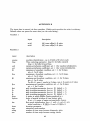
APPENDIX B
The input data is entered via four namelists. Within each namelist the order is arbitrary.
Default values are preset for most data (see the code listing).
Namelist 1
input
description
nold
n03d
1[0] turns off[on] I-D plots
1[0] turns off[on] 3-D plots
Namelist 2
input
aname
bias
exO
exl
fil
fizx
fjl
fjrx
fpsi
fu
fv
fz
jfour
kplotm
kzs
lmax
mm
ndiag
n.en
description
problem identification , up to 5 fields of 8 letters each
Time centering parameter. biaseeO. for fully centered
bias=1. for fully forward bias.
initial perturbation coefficient, set = 1 for random initialization.
initial perturbation coefficient, set = 1 for cosine initialization.
minimum z boundary condition, set = 1. for 0 slope,
set=-I. for 0 value
maximum z boundary condition, set == 1. for 0 slope,
set=-1. for 0 value
minimum psi boundary condition. set = 1. for 0 slope,
set=-1. for 0 value
For fjl=O., mm=1 results in 0 slope, mm ~ 2 results in 0 value
maximum psi boundary condition, set =1. for 0 slope,
set =-1. for 0 value
grid stretching parameter (see sec. 9). default = .5
grid stretching parameter (see sec. 9). default = .5
grid stretching parameter (see sec. 9). default = .5
grid stretching parameter (see sec. 9). default = .5
1ft index at which XROis Fourier-analyzed in z
index of spatial location of time history plots.
If set == 0, center of region automatically chosen.
flute mode initialization. kzs = 1 ,exO =1., exl=O. sets
initial condition, r B XRO= O.,and r B XIO= O.
iteration parameter
azimuthal mode number
number of time steps between diagnositc plots
number of time steps between energy checks
16
Narnelist 2 continued
input
description
nfourmax
no. of times the buffer is read to the history file
for Fourier analysis
Fourier analyze XROevery nfourp'th . time step
total number of time steps for problem
arbitrary scaling factor on the gyroscopic fir term XXX
arbitrary scaling factor on the quasi-elastic fir term YYY
arbitrary scaling factor on the curvature-drive term
default=1
arbitrary scaling factor on some of the line-bending terms
default = 1
arbitrary scaling factor on some of the line-bending terms
default = 1
arbitrary scaling factor on some of the line-bending terms
default = 1
nfourp
nmax
sm
sf8
swg l
swg2
swg3
swg4.
Namelist 3
input
description
bceng
betcene
betcent
betpasl
betrap
betring
betslse
betslsh
cold
center cell magnetic field in Gauss
peak center cell electron j3..L
peak centew cell ian j3..L
center cell passing j3
peak choke cell j3..L
peak hot electron j3..L
peak warm sloshing electron j3..L
peak sloshing ion j3..L
a global density minimum as a fraction of ncenter,
the center cell density
parameter in 1/1 pressure profile (sec. 8)
center cell passing density
1/1 width relative to 1/1max of transition
to halo region
peak density in choke cell
ion charge . Default=4.8e-1O
used for elongated hot electrons. See sec A.3
switch which sets hot electron z-length as
elongated (long=l) or regular (Iong=O)
center cell density [particlca/cm"]
peak plug cell density (particlea/cm")
dip
dpasl
dpsihrel
dltrap
echarg
fring
long
ncenter
nsloshin
17
Namelist 3 continued
input
pelO
ppas2
ppas3
psiOrel
psiOerel
psihrrel
psislp
psi3rel
p2wide
p2ewide
plf1.oor
p2f1.ag
p2f1.oor
rpl
rw
rwl
wpot
xpot
ypot
z3rel
description
coefficient of hot electron radial pressure
profile (sec. 8)
minimum passing pressure in the choke cell, expressed
as a fraction of ppasl (sec. 7)
maximum passing pressure at the inboard mirror of the
end plug cell
1/J value relative to 1/Jmax at which
ion radial pressure is half the maximum.
1/J value relative to 1/Jmax at which
hot electron radial pressure fs half the maximum.
1/J value relative to 1/Jmax of halo.
coefficient of Pel (sec. 8 )
1/J value relative to 1/Jmax beyond which electric field=O
parameter inversly proportional to ramp width of PZt
the ion radial pressure profile (sec. 8)
parameter inversly proportional to ramp width of PZe
'the hot electron radial pressure profile (sec. 8)
value to which PI is set if PZ :::; p2jlag
value of PZ at which PI and PZ are set constant
value to which PZ is set if PZ ~ p2jlag
mirror ratio of the inner component of the sloshing profile (sec. 6)
wall radius in em.·
slightly less , within one grid cell, or equal to wall radius rw
exponent coefficient in end plug cell potential
exponent coefficient in center cell potential
power of polynomial in potential 1/J dependence
outer axial position where hot electrons go to 0
Namelist 4
input
description
als
as
bmxl
bmx2
three element array of z location of each solenoid center
three element array of radius of each solenoid
magnetic field at the choke coil solenoid (Gauss), (sec. 3)
magnetic field at the inboard end plug solenoid, (Gauss),(sec. 3)
18
Namelist 4 continued
input
description
bmx3
bceng
dt
dphi
epsp
magnetic field at the outer end plug solenoid, (Gauss),(sec. 3)
magnetic field in center cell (Gauss)
time step (sec.)
Ignore
~ minimum pressure (normalized to 1 ), below which
B is calculated by an expansion . see sec AA
number of points used in Simpson's quadrature for r z z .default=23
transition length for central cell vacuum
number of solenoid coils (also regions)
maximum electric potential in center cell
maximum electric potential in end plug cell
parameter on sloshing shape. default =0.
Ignore
maximum z of the domain
z location of choke solenoid
z location of end plug inboard solenoid
z location of end plug outer solenoid
kin
ltrans
ncoil
phicen
phiplg
pfudge
thetaO
zmax
zlc
z2c
z3c
19
Technical Information Department- Lawrence Livermore National Laboratory
University of California . Livermore, California 94550