1
arXiv:1410.3012 LU TP 14-36 MCNET-14-22 CERN-PH-TH-2014-190 FERMILAB-PUB-14-316-CD DESY 14-178 SLAC-PUB-16122 October 2014 An Introduction to PYTHIA 8.2 Torbjörn Sjöstranda,∗, Stefan Askb,1 , Jesper R. Christiansena , Richard Corkea,2 , Nishita Desaic , Philip Iltend , Stephen Mrennae , Stefan Prestelf,g , Christine O. Rasmussena , Peter Z. Skandsh,i a Department of Astronomy and Theoretical Physics, Lund University, Sölvegatan 14A, SE-223 62 Lund, Sweden b Department of Physics, University of Cambridge, Cambridge, UK c Institut für Theoretische Physik, Universität Heidelberg, Philosophenweg 16, D-69120 Heidelberg, Germany d Massachusetts Institute of Technology, Cambridge, MA 02139, USA e Fermi National Accelerator Laboratory, Batavia, IL 60510, USA f Theory Group, DESY, Notkestrasse 85, D-22607 Hamburg, Germany g SLAC National Accelerator Laboratory, Menlo Park, CA 94025, USA h CERN/PH, CH–1211 Geneva 23, Switzerland i School of Physics, Monash University, PO Box 27, 3800 Melbourne, Australia Abstract The Pythia program is a standard tool for the generation of events in high-energy collisions, comprising a coherent set of physics models for the evolution from a few-body hard process to a complex multiparticle final state. It contains a library of hard processes, models for initial- and final-state parton showers, matching and merging methods between hard processes and parton showers, multiparton interactions, beam remnants, string fragmentation and particle decays. It also has a set of utilities and several interfaces to external programs. Pythia 8.2 is the second main release after the complete rewrite from Fortran to C++, and now has reached such a maturity that it offers a complete replacement for most applications, notably for LHC physics studies. The many new features should allow an improved description of data. ∗ Corresponding author; e-mail address: [email protected] Now at Winton Capital Management, Zurich, Switzerland 2 Now at Nordea Bank, Copenhagen, Denmark 1 Preprint submitted to Computer Physics Communications October 14, 2014 Keywords: event generators, multiparticle production, matrix elements, parton showers, matching and merging, multiparton interactions, hadronisation 2 NEW VERSION PROGRAM SUMMARY Manuscript Title: An Introduction to Pythia 8.2 Authors: Torbjörn Sjöstrand, Stefan Ask, Jesper R. Christiansen, Richard Corke, Nishita Desai, Philip Ilten, Stephen Mrenna, Stefan Prestel, Christine O. Rasmussen, Peter Z. Skands Program Title: Pythia 8.2 Journal Reference: Catalogue identifier: Licensing provisions: GPL version 2 Programming language: C++ Computer: commodity PCs, Macs Operating systems: Linux, OS X; should also work on other systems RAM: ∼10 megabytes Keywords: event generators, multiparticle production, matrix elements, parton showers, matching and merging, multiparton interactions, hadronisation Classification: 11.2 Phase Space and Event Simulation Catalogue identifier of previous version: ACTU v3 0 Journal reference of previous version: T. Sjöstrand, S. Mrenna and P. Skands, Computer Physics Commun. 178 (2008) 852 Does the new version supersede the previous version?: yes Nature of problem: high-energy collisions between elementary particles normally give rise to complex final states, with large multiplicities of hadrons, leptons, photons and neutrinos. The relation between these final states and the underlying physics description is not a simple one, for two main reasons. Firstly, we do not even in principle have a complete understanding of the physics. Secondly, any analytical approach is made intractable by the large multiplicities. Solution method: complete events are generated by Monte Carlo methods. The complexity is mastered by a subdivision of the full problem into a set of simpler separate tasks. All main aspects of the events are simulated, such as hard-process selection, initial- and final-state radiation, beam remnants, fragmentation, decays, and so on. Therefore events should be directly comparable with experimentally observable ones. The programs can be used to extract physics from comparisons with existing data, or to study physics at future experiments. Reasons for the new version: improved and expanded physics models Summary of revisions: hundreds of new features and bug fixes, allowing an improved modeling Restrictions: depends on the problem studied Unusual features: none Running time: 10–1000 events per second, depending on process studied 3 1. Introduction The Pythia program is a standard tool for the generation of events in high-energy collisions between elementary particles, comprising a coherent set of physics models for the evolution from a few-body hard-scattering process to a complex multiparticle final state. Parts of the physics have been rigorously derived from theory, while other parts are based on phenomenological models, with parameters to be determined from data. Currently the largest user community can be found among the LHC experimentalists, but the program is also used for a multitude of other phenomenological or experimental studies. Main tasks performed by the program include the exploration of experimental consequences of theoretical models, the development of search strategies, the interpretation of experimental data, and the study of detector performance. Thereby it spans the whole lifetime of an experiment, from early design concepts for the detector to final presentation of data. The development of Jetset [1, 2, 3, 4] began in 1978 and many of its components were merged later with Pythia [5, 6, 7, 8, 9, 10]. Thus the current Pythia generator is the product of more than 35 years of development. At the onset, all code was written in Fortran 77. Pythia 8.100 [11] was the first full release of a complete rewrite to C++. As such, some relevant features were still missing, and the code had not yet been tested and tuned to the same level of maturity as Pythia 6.4 [10], the last version of the old Fortran generation. Since then missing features have been added, new features introduced, and bugs found and fixed. Experience has been building slowly in the experimental community and the LHC collaborations, in particular, are in the midst of or have made the full-scale transition from Pythia 6 to Pythia 8. The development of Pythia 8.1 after the original release has been a continuous process, and backwards incompatibility has been introduced in only a few instances. We take the opportunity of the Pythia 8.200 release to introduce a further set of minor incompatibilities, in particular to remove some outdated functionality. Most user programs should work unchanged, or only require minimal adjustments. On the one hand, Pythia is intended to be self-contained, useful for any number of standalone physics studies. On the other, an ongoing trend is that Pythia 8 is interlinked with other program packages. This is accomplished through a number of interfaces, with the Les Houches Accord (LHA) [12] and its associated Les Houches Event Files (LHEF) [13, 14] being a prime example. In this way, matrix-element (ME) based calculations from a number of different sources can be combined with Pythia specialities such as initial-state radiation (ISR), final-state radiation (FSR), multiparton interactions (MPI), and string fragmentation. The intention of this article is neither to provide a complete overview of the physics implemented, nor a complete user manual describing, for example, the complete set of runtime settings. This was done for Pythia 6.4, and required 580 pages [10]. For Pythia 8 the user manual part is completely covered by a set of interlinked HTML (or alternatively PHP) pages that is distributed along with the program code. In addition there is a worksheet, intended for summer schools or self-study, that offers an introductory tutorial, and example main programs to get started with various tasks. For the physics implementation, the story is more complex. Major parts of the Pythia 6.4 writeup still are relevant, but there are also parts that have evolved further 4 since. This is only briefly covered in the HTML manual. In the future we intend to link more PDF documents with detailed physics descriptions to it, but this will be a slow buildup process. The intention here is to provide information that explains the evolution of the current program and makes the other resources, such as the online manual, intelligible. Section 2 contains a concise summary of the physics of Pythia 8, with emphasis on limitations and on aspects that are new since Pythia 8.100. A short overview of the program code follows in section 3 that includes installation instructions, an outline of the main program elements, methods for user interaction with the code, the possibility of interfaces with external libraries, and more. Section 4 rounds off the article with an outlook to future developments. 2. Physics Summary As described in the introduction, only a brief outline of the physics content will be provided here, with emphasis on those aspects that are new since Pythia 8.100 and on Pythia’s area of application, since many user questions concern what Pythia cannot do. Further details are available in the HTML manual, and in a number of physics publications over the years, notably the Pythia 6.4 manual [10]. 2.1. Limitations The physics models embodied in Pythia focus on high-energy particle collisions, defined as having centre-of-mass (CM) energies greater than 10 GeV, corresponding to a proton–proton (pp) fixed-target beam energy of ≥ 50 GeV. This limitation is due to the approximation of a continuum of allowed final states being used in several places in Pythia, most notably for hadron–hadron cross-section calculations, total and differential, and as the basis for the string-fragmentation model. At energies below 10 GeV, we enter the hadronic resonance region, where these approximations break down, and hence the results produced by Pythia would not be reliable. The 10 GeV limit is picked as a typical scale; for positron–electron (e+ e− ) annihilation it would be possible to go somewhat lower, whereas for pp collisions the models are not particularly trustworthy near the lower limit. At the opposite extreme, we are only aware of explicit tests of Pythia’s physics modeling up to CM energies of roughly 100 TeV, corresponding to a pp fixed-target beam energy ≤ 1010 GeV; see e.g. [15, 16]. Using Pythia to extrapolate to even higher energies is not advised for novice users and should be accompanied by careful cross checks of the modeling and results. Currently the program only works either with hadron–hadron or lepton–lepton collisions. Hadron here includes the (anti)proton, (anti)neutron, pion and, as a special case, the Pomeron. There is not yet any provision for lepton–hadron collisions or for incoming photon beams, though these could conceivably be added in future significant updates. Internal facilities to handle proton–nucleus or nucleus–nucleus collisions are not foreseen at all. For completeness, however, we note that a wide range of programs exist with interfaces to some of the physics models in Pythia, in particular the string fragmentation routines, for collision and decay processes. 5 The outgoing particles are produced in vacuum and the simulation of the interaction of the produced particles with detector material is not included in Pythia. Interfaces to external detector-simulation codes can be written directly by the user or accomplished via the HepMC [17] interface, as described in subsection 3.8.12. Analysis of Pythia events can always be done at the parton or particle level. Examples of such analyses are provided with the code distribution. 2.2. Hard processes A large number of processes are available internally, and even more through interfaces to external programs. The input of external hard processes via the LHA/LHEF standards actually is the main source of a rapidly expanding set of processes that Pythia can handle. Nevertheless there will always remain some need for internal processes, in part the standard ones required for basic physics studies, in part ones with special requirements, like involving long-lived coloured particles, new colour structures, or parton showers in new gauge groups. Recent internal additions include several scenarios for Hidden Valley physics, further processes involving extra dimensions, more Supersymmetric (SUSY) processes, extended handling of R-hadrons, and more charmonium/bottomonium states. The implementation of hard processes focuses on 2 → 1 and 2 → 2 processes with some 2 → 3 processes available. It may be possible however, to generate processes with higher final-state multiplicity if the particles arise from decays of resonances. As of version 8.2, the following processes are available internally: • QCD processes include both soft- and hard-QCD processes. The hard-QCD processes include the standard 2 → 2 ones available in Pythia 6.4, with open charm and bottom production, as well as new 2 → 3 processes that can be used, for example, for comparisons with parton showers. • Electroweak (EW) processes include prompt photon production, single production of γ ∗ /Z and W± as well as pair production of weak bosons with full fermion correlations for V V → 4f. Photon collision processes of the type γγ → ff are also available. • Onia include production of any 3 S1 , 3 PJ and 3 DJ states of charmonium or bottomonium via colour-singlet and colour-octet mechanisms. • Top production, singly or in pairs. • Fourth generation fermion production via strong or EW interactions. • Higgs processes include the production of the SM Higgs boson as well as the multiple Higgs bosons of a generic two-Higgs-doublet model (2HDM), with the possibility of CP violating decays. It is also possible to modify the angular correlation of the Higgs decay h → V V → 4f due to anomalous hV V couplings. The internal implementation of SUSY also uses the 2HDM implementation for its Higgs sector. • SUSY processes include the pair production of SUSY particles as well as resonant production of squarks via the R-parity violating UDD interaction. EW interferences 6 have been taken into account where relevant and can be turned off for comparisons with Pythia 6.4. The implementation has been documented in [18]. Both squarks and gluinos can be made to form long-lived R-hadrons, that subsequently decay. In between it is possible to change the ordinary-flavour content of the R-hadrons, by (user-implemented) interactions with the detector material [19]. • New gauge boson processes include production of a Z0 (with full γ ∗ /Z/Z0 interference), a W0± and of a horizontally-coupling (between generations) gauge boson R0 . ± • Left-right symmetric processes include the production of the SU (2)R bosons WR , ++ Z0R , and the doubly charged Higgs bosons H++ and H . L R • Leptoquark production, singly or in pairs, with the assumption that the leptoquark always decays before fragmentation. • Compositeness processes include the production of excited fermions and the presence of contact interactions in QCD or EW processes. The production of excited fermions can be via both gauge and contact interactions; however, only decays via gauge interactions are supported with angular correlation. • Hidden Valley processes can be used to study visible consequences of radiation in a hidden sector. Showering is modified to include a third kind of radiation, fully interleaved with the QCD and QED radiation of the SM. New particles include SU (N )charged gauge bosons as well as partners of the SM fermions charged under SU (N ). See [20, 21] for further details. • Extra-dimension processes include the production of particles predicted by Randall-Sundrum models, TeV-sized and Large Extra Dimensions, and Unparticles. See [22, 23, 24] for detailed descriptions. The full list of available processes and parameters for BSM models along with references is available in the HTML manual distributed with the code. Furthermore, for the cases of one, two, or three hard partons/particles in the final state, the user can also use the Pythia class structure to code matrix elements for required processes as yet unavailable internally, and even use MadGraph 5 [25] to automatically generate such code. This is discussed later in subsection 3.8.4. 2.3. Soft processes Pythia is intended to describe all components of the total cross section in hadronic collisions, including elastic, diffractive and non-diffractive topologies. Traditionally special emphasis is put on the latter class, which constitutes the major part of the total cross section. In recent years the modeling of diffraction has improved to a comparable level, even if tuning of the related free parameters is lagging behind. The total, elastic, and inelastic cross sections are obtained from Regge fits to data. At the time of writing, the default for pp collisions is the 1992 Donnachie-Landshoff parametrisation [26], with one Pomeron and one Reggeon term, pp σTOT (s) = (21.70 s0.0808 + 56.08 s−0.4525 ) mb, 7 (1) with the pp CM energy squared, s, in units of GeV2 . For pp collisions, the coefficient of the second (Reggeon) term changes to 98.39; see [26, 27, 10] for other beam types. The elastic cross section is approximated by a simple exponential falloff with momentum transfer, valid at small Mandelstam t, related to the total cross section via the optical theorem, pp pp dσEL (σTOT )2 (s) pp = exp (BEL (s) t) dt 16π → pp σEL (s) = pp (σTOT )2 , pp 16πBEL (s) (2) pp using 1 mb = 1/(0.3894 GeV2 ) to convert between mb and GeV units, and BEL = 5+4s0.0808 −2 the pp elastic slope in GeV , defined using the same power of s as the Pomeron term in σTOT , to maintain sensible asymptotic behaviour at high energies. We emphasise that also the electromagnetic Coulomb term, with interference, can optionally be switched on for elastic scattering — a feature so far unique to Pythia among major generators. The inelastic cross section is a derived quantity: σINEL (s) = σTOT (s) − σEL (s) . (3) The relative breakdown of the inelastic cross section into single-diffractive (SD), doublediffractive (DD), central-diffractive (CD), and non-diffractive (ND) components is given by a choice between 5 different parametrisations [28, 29]. The current default is the SchulerSjöstrand one [27, 30]: pp→Xp 3 dσSD (s) g3P βpP Xp = FSD (MX ) exp BSD t , dt dMX2 16π MX2 (4) pp 2 2 βpP dσDD (s) g3P = FDD (M1 , M2 ) exp (BDD t) , dt dM12 dM22 16π M12 M22 (5) with the diffractive masses (MX , M1 , M2 ), the Pomeron couplings (g3P , βpP ), the diffractive slopes (BSD , BDD ), and the low-mass resonance-region enhancement and high-mass kinematical-limit suppression factors (FSD , FDD ) summarised in [28]. The central-diffractive component is a new addition, not originally included in [28]. By default, it is parametrised according to a simple scaling assumption, σCD (s) = σCD (sref ) ln(0.06 s/s0 ) ln(0.06 sref /s0 ) 3/2 , with σCD (sref ) the CD cross section at a fixed reference CM energy chosen to be √ 2 TeV by default and s0 = 1 GeV. The spectrum is distributed according to pp dσCD (s) 1 pX Xp ∝ exp BSD t1 exp BSD t2 , dt1 dt2 dξ1 dξ2 ξ1 ξ2 (6) √ sref = (7) with ξ1,2 being the fraction of the proton √ energy carried away by the Pomeron, related to the diffractive mass through MCD = ξ1 ξ2 s. 8 Depending on the selected diffractive parametrisation, the non-diffractive cross section is evaluated by integrating the diffractive components and subtracting them from σINEL , Z pp pp pp→Xp pp→pX pp pp σND (s) = σINEL (s) − dσSD (s) + dσSD (s) + dσDD (s) + dσCD (s) . (8) Note, therefore, that the ND cross section is only defined implicitly, via eqs. (3) – (8). We emphasise that recent precision measurements at high energies, in particular by TOTEM [31, 32] and by ALPHA [33], have highlighted that σTOT (s) and σEL (s) actually grow a bit faster at large s, while σINEL (s) remains in the right ballpark. More recent fits [34, 35] are consistent with using a power s0.096 for the Pomeron term. Updating the total cross-section formulae in Pythia 8 is on the to-do list for a future revision. Alternatively, it is also possible to set your own user-defined cross sections (values only, not functional forms), see the HTML manual’s section on “Total Cross Sections”. Among the event classes, the non-diffractive one is the norm, in the context of which most aspects of event generators have been developed. It is therefore amply covered in subsequent sections. Single, double and central diffraction now are handled in the spirit of the Ingelman– Schlein model [36], wherein a Pomeron is viewed as glueball-like hadronic state. The Pomeron flux defines the mass spectrum of diffractive systems, whereas the internal structure of this system is simulated in the spirit of a non-diffractive hadronic collision between a Pomeron and a proton [28]. Low-mass diffractive systems are still assumed to exhibit no perturbative effects and hence are represented as purely non-perturbative hadronizing strings, respecting the quantum numbers of the diffractively excited hadrons and with phenomenological parameters governing the choice between two different possible string configurations. For diffractive systems with masses greater than about 10 GeV (a user-modifiable smooth transition scale), ISR and FSR effects are fully included, hence diffractive jets are showered, and the additional possibility of MPI within the Pomeron–proton system allows for an underlying event to be generated within the diffractive system. Exclusive diffractive processes, like pp → pph, with h representing a single hadron, have not been implemented and would in any case not profit from the full Pythia machinery. 2.4. Parton distributions Currently, sixteen parton distribution function (PDF) sets for the proton come builtin. In addition to the internal proton sets, a few sets are also available for the pion, the Pomeron, and the leptons. The Q2 evolution of most of these sets is based on interpolation of a grid. A larger selection of PDFs can be obtained via the interfaces to the LHAPDF libraries, one to the older Fortran-based LHAPDF5 [37] and one to the newer C++-based LHAPDF6 [38]. Given that the Pythia machinery basically is a leading-order (LO) one, preference has been given to implementing LO sets internally. In a LO framework, the PDFs have a clear physical interpretation as the number density of partons, and can be related directly to measurable quantities. In the modeling of minimum bias (MB) and underlying event (UE) phenomena, very small x scales are probed, down to around 10−8 , for Q scales that may go below 1 GeV. Measurements of F2 imply a small-x behaviour for gluon and sea quark PDFs where xfi (x, Q2 ) is constant or even slowly rising for x → 0 at a fixed Q2 around 9 1 − 4 GeV2 . This behaviour is evident in LO PDF fits. Next-to-leading-order (NLO) PDFs, on the other hand, no longer have a probabilistic interpretation, and their behaviour is less directly related to physical quantities. They have small-x corrections proportional to ln(1/x), that may drive PDFs negative at small x and Q. This makes them unsuitable for describing showers or MPIs. Contrary to this argument, event tunes have been produced with NLO PDFs that give a reasonable description of available collider data. However, this is likely related to the resiliency of the MPI and string fragmentation frameworks, which allow a rather significant change of PDF shape to be compensated by a retuning of relevant parameters. What is notable is that these NLO tunes require a significantly smaller p⊥0 scale, where p⊥0 is used to tame the 1/p4⊥ divergence of the QCD cross sections to 1/(p2⊥ + p2⊥0 )2 . This reduced p⊥0 compensates for the low amount of small-x gluons in NLO PDFs. Since the integrated QCD cross sections depend on the number density fi (x, Q2 ), the small-x partons play an important role in determining the number and kinematics of the MPIs. In the NLO tunes, the MPI collisions would tend to be symmetric, i.e. x1 ∼ x2 , and both not too small. Asymmetric collisions, where one x is small, would be suppressed by the respective NLO PDFs vanishing or at least being tiny there (a negative PDF is reset to 0 in Pythia). With further scrutiny, one expects to find differences in the rapidity spectrum of minijets from MPIs. Irrespective of that, there is no reason to use NLO PDFs in regions where they are known not to be trustworthy. If one is not satisfied to use a LO PDF set throughout, Pythia offers the possibility to use two separate PDF sets; one for the hard interaction and one for the subsequent showers and MPI. The former could well be chosen to be NLO and the latter LO. Recall, also, that ISR generated with the standard backwards evolution scheme is based on ratios of PDFs. Therefore many of the differences between PDF sets divide out, notably away from the low-x region. An additional advantage of a two-PDF setup is that it becomes possible to explore a range of PDFs for the hard process without any necessity to redo the UE/MB tune. Some PDF studies in the Pythia context are found in [39]. 2.5. Parton showers The ISR and FSR algorithms are based on the dipole-style p⊥ -ordered evolution first introduced in Pythia 6.3 [40]. New features in Pythia 8 include γ → qq and γ → `+ `− branchings as part of the FSR machinery, options for emission of weak gauge bosons, Z0 and W± , as part of both ISR and FSR [41], extensions of the shower framework to handle bremsstrahlung in Hidden Valley models [20, 21], and flexible colour strengths for FSR when the emission rate is to be shared between several recoilers [18], used e.g. to describe radiation in R-parity violating SUSY decays. Options also exist for alternative FSR recoil schemes and for gluon emissions off colour-octet onium states. The entire perturbative evolution (ISR, FSR, and MPI) is interleaved into a single common sequence of decreasing p⊥ [42]. The full interleaving performed in Pythia 8, which can be switched on/off for cross checks, has the beneficial consequence that the phase space available to hard FSR emissions cannot end up depending on dipoles created by soft ISR ones, hence we regard the new algorithm as more theoretically consistent. Instead, some FSR is associated with colour dipoles stretched between a final-state parton 10 and the beam-remnant ”hole” left by an initial-state one, which therefore now can take a recoil. In the ISR algorithm, recoils are always taken by the hard-scattering subsystem as a whole, regardless of whether the colour partner is in the initial or final state. The shower evolution is based on the standard (LO) DGLAP splitting kernels, P (z) [43, 44, 45]: 1 + z2 , 1−z (1 − z(1 − z))2 Pg→gg (z) = CA , z(1 − z) Pg→qq̄ (z) = TR (z 2 + (1 − z)2 ) , Pq→qg (z) = CF (9) (10) (11) with CF = 34 , CA = NC = 3, and TR = 12 , multiplied by Nf if summing over all contributing quark flavours, for QCD, and 1 + z2 , 1−z Pγ→f f̄ (z) = e2f NC (z 2 + (1 − z)2 ) , Pf→fγ (z) = e2f (12) (13) for QED, with NC = 1 for charged leptons, and with z the energy-sharing fraction between the daughter partons. In addition, the current default is that gluon-polarisation effects are taken approximately into account via a non-isotropic selection of the azimuthal angle of the branchings, ϕ. Corrections for parton masses are generally also included, for both FSR [46] and ISR [40]. Additional options for mass corrections for g/γ → f f̄ branchings are discussed below. The ISR and FSR algorithms are both based on the above splitting kernels, and are cast as differential equations expressing the probability of emitting radiation as one moves from high to low values of the shower evolution variable, which plays the role of factorisation scale in parton-shower contexts. For FSR, this corresponds to an evolution forwards in physical time, with a single mother parton replaced by two daughter partons at each branching. For ISR, however, the progress from high to low factorisation scales corresponds to a backwards evolution in physical time [47], with the evolving parton becoming unresolved into a new initial-state mother parton and an accompanying final-state sister one at each branching. Moreover, the fact that the boundary condition represented by the non-perturbative structure of the initial beam particle sits at the low-Q end of the evolution chain implies that a ratio of PDFs accompanies each branching, with the purpose, roughly, of translating from the PDF of the ”old” mother parton to that of the ”new” one. Integrated over the kinematically allowed range of z and expressed as a differential branching probability per unit evolution time, the FSR and ISR kernels used to drive the shower evolution in Pythia are: Z dPFSR 1 αs = 2 dz P (z) , 2 dp⊥ p⊥ 2π Z dPISR 1 αs f 0 (x/z, p2⊥ ) = dz P (z) , (14) dp2⊥ p2⊥ 2π zf (x, p2⊥ ) 11 with z = x/x0 for ISR defined so x < x0 , and the Pythia transverse-momentum evolution variable defined by (1 − z)Q2 : ISR 2 2 p⊥ = p⊥evol = , (15) z(1 − z)Q2 : FSR with Q2 the offshellness of the branching parton: Q2FSR = (p2 − m20 ) and Q2ISR = (−p2 + m20 ), determined for each branching by solving the above equation for Q2 . Note that, since FSR branchings involve timelike virtualities (p2 > 0) while ISR ones involve spacelike virtualities (p2 < 0), both Q2 definitions correspond to positive-definite quantities. The overall strength of radiation is set by the effective value of αs (MZ ), which can be specified separately for ISR and FSR. Although nature contains only a single strong coupling, the structure of higher-order splitting kernels differs between ISR and FSR, and a further subtlety is that ISR involves an interplay with PDFs, while FSR does not. Hence we believe there is ample justification for maintaining two distinct effective αs (MZ ) values for bremsstrahlung, in addition to the ones which govern hard processes and MPI. The default renormalisation scale used to evaluate αs for each shower branching is the shower evolution scale, p⊥evol . For gluon-emission processes, this is the canonical choice of renormalisation scale [48], and it yields the correct O(αs2 ln3 ) behaviour at the integrated level. Optionally, a multiplicative prefactor can be applied, µ2R = kµR p2⊥evol , with default value kµR = 1. This can be varied, e.g., to perform uncertainty estimates. We emphasise that the αs (MZ ) values used for ISR and FSR in Pythia are not directly comparable to the MS αs (MZ ) = 0.1185(6) given by the PDG [49], for two reasons. Firstly, in the limit of soft-gluon emission (z → 1), it can be shown that the dominant O(αs2 ) splitting-function term, which generates contributions starting from O(αs2 ln2 ) at the integrated level, can be absorbed into the LO splitting functions by translating to the so-called CMW (a.k.a. MC) scheme [50], αs αs αsMC = αsMS 1 + K ←→ αsMS = αsMC 1 − K , (16) 2π 2π where the scheme choice for the αs /2π correction terms amounts to an O(αs3 ) effect, and 4.565 : Nf = 3 67 1 2 5 4.010 : Nf = 4 K = CA − π − Nf = , (17) 3.454 : Nf = 5 18 6 9 2.899 : Nf = 6 with CA = 3 and Nf the number of contributing quark flavours. The baseline value to use for shower αs (MZ ) values should therefore be around αs (MZ )MC = 0.126. Secondly, even this larger value of αs only takes into account the NLO correction to the splitting kernel in the infinitely soft limit. In the rest of phase space, the remaining NLO corrections still tend to be positive, see e.g. [51], and hence the effective value of αs (MZ ), when tuned directly to data, tends to be a further 10% larger, at αs (MZ )PYTHIA ∼ 0.139. In Pythia, one has the option of letting the translation between the MS and MC schemes be done automatically, though the default is just to provide an effective αs (MZ ) 12 value directly in the Pythia scheme. We also note that the arguments in [50] were based on 2-loop running, while the default in Pythia is to use 1-loop running, which gives lower ΛQCD values, allowing lower shower cutoffs to be used. For g → qq and γ → f f̄ splitting processes, the alternative choice of using µR ∝ mf f̄ has also recently been implemented, along with several options for the handling of mass effects, notably for charm and bottom quarks. The default now is to start out from a splitting kernel, P (z) = z 2 + (1 − z)2 + 8rf z(1 − z) , (18) normalised so that the z-integrated rate is (βf /3)(1 + rf /2), with rf = m2f /m2ff̄ and βf = √ 1 − 4rf , which should be the correct infinite-energy expression. This is then modified for finite dipole masses by an (1 − m2ff̄ /m2dipole )3 suppression factor, a factor which is derived from the H0 → gg → qqg matrix element, but should be a reasonable estimate also for other processes. Concerning the emission of hard extra jets, one should be aware that the parton-shower machinery is primarily intended to describe physics near the collinear and/or soft limits, in which successive radiation p⊥ scales are strongly ordered. Nevertheless, an extensive set of automated matrix-element corrections have been implemented, which correct the first jet emission to the full LO matrix-element expression for a wide range of production and decay processes, see [52, 46]. For these processes, Pythia is therefore expected to achieve LO accuracy out of the box also for hard radiation. For the FSR algorithm such corrections are applied by default to all 1 → 2 decay processes in the SM and many BSM ones [46]. For the ISR shower, internal ME corrections have so far only been implemented for radiation in a few hard 2 → 1 processes, specifically (Z/W/H) + jet [52]. For all other processes, an approximate improved-shower description is used to ensure a reasonable behaviour up to the kinematic limit at high p⊥ scales [53]. Alternatively, see subsection 2.10 below for information on matching and merging using external ME generators. Finally, in the context of uncertainty estimates, it is worth noting that the MS → MC scheme translation is equivalent to making a specific shift of renormalisation scale, µR → µR exp(−K/4πβ0 ) ∼ µR /1.6 (for Nf = 5), with β0 = (11CA − 2Nf )/(12π) the 1-loop beta function in QCD and K defined by eq. (17). Therefore, making arbitrary variations of µR around this scale will actually spoil the NLL precision of the shower, at least in the infinitely soft limit in which the translation is derived. So far, Pythia does not automatically attempt to compensate for this, leaving it up to the user to judge which variations to consider reasonable. 2.6. Multiparton interactions In hadron–hadron collisions, MPI are a natural consequence of the composite structure of the colliding beam particles. Although MPI are especially relevant to describe the ubiquitous soft underlying event, the possibility of having several hard scattering processes occurring in one and the same hadron–hadron collision also exists, albeit at suppressed rates relative to soft MPI. The basic formalism underpinning the MPI modeling in Pythia is described in [54] and spans both soft and hard QCD MPI processes in a single unified framework. The current implementation, summarised briefly below, further contains the additional refinements introduced since Pythia 6.3 [55], along with a few new additions unique to Pythia 8. In 13 particular, the mix of MPI processes has been enlarged from covering only partonic QCD 2 → 2 scattering in Pythia 6 to also allowing for multiple γ + jet and γγ processes, coloursinglet and -octet charmonium and bottomonium production, s-channel γ exchange, and t-channel γ/Z0 /W± exchange. Note also that for dedicated studies of two low-rate processes in coincidence, the user can now request two distinct hard interactions in the same event, with further MPI occurring as usual. There are then no Sudakov factors included for these two interactions, similarly to normal events with one hard interaction. The starting point for parton-based MPI models is the observation that the t-channel propagators and αs factors appearing in perturbative QCD 2 → 2 scattering diverge at low momentum transfers, 2 gs4 dt 2 2 dp⊥ dσ2→2 ∝ ∼ α (p ) , (19) s ⊥ 16π 2 t2 p4⊥ a behaviour further √ exacerbated by the abundance of low-x partons that can be accessed at large hadronic s. At LHC energies, this parton–parton cross section, integrated from some fixed p⊥min scale up to the kinematic maximum, becomes larger than the total hadron– hadron cross section for p⊥min values of order 4 − 5 GeV. In the context of MPI models, this is interpreted straightforwardly to mean that each hadron–hadron collision contains several parton–parton collisions, with typical momentum transfers of the latter of order p⊥min . This simple reinterpretation in fact expresses unitarity; instead of the total interaction cross section diverging as p⊥min → 0, which would violate unitarity, we have restated the problem so that it is now the number of MPI per collision that diverges, while the total cross section remains finite. Taking effects beyond (unitarised) 2 → 2 perturbation theory into account, the rise of the parton–parton cross section for p⊥ → 0 must ultimately be tamed by colour-screening effects; the individual coloured constituents of hadrons cannot be resolved by infinitely long (transverse) wavelengths, analogously to how hadronisation provides a natural lower cutoff for the perturbative parton-shower evolution. In Pythia, rather than attempting an explicit dynamical modeling of screening and/or saturation effects, this aspect is implemented via the effective replacement, αs2 (p2⊥ ) αs2 (p2⊥ + p2⊥0 ) dσ2→2 ∝ → , dp2⊥ p4⊥ (p2⊥ + p2⊥0 )2 (20) which smoothly regulates the divergence. The MPI cross section in the p⊥ → 0 limit thus tends to a constant, the size of which is controlled directly by: 1. the effective p⊥0 parameter, 2. the value of αs (MZ ) used for MPI and its running order, and 3. the PDF set used to provide the parton luminosities for MPI. These are therefore the three main tunable aspects of the model. Two further highly important ones are the assumed shape of the hadron mass distribution in impact-parameter space, and the strength and modeling of colour-reconnection effects. To be more explicit, the regulated parton–parton cross section, eq. (20), can be integrated to provide a first rough estimate of how many MPI, on average, occur in each 14 (average, inelastic non-diffractive) hadron–hadron collision, hnMPI i(p⊥0 ) = σ2→2 (p⊥0 ) , σND (21) with σND given by eq. (8). This formula would only be strictly true if all the MPI could be considered equivalent and independent, i.e. uncorrelated, in which case hnMPI i could be interpreted as the mean of a Poisson distribution. In Pythia, this is not the case, since several correlation effects are taken into account, some of which can be quite important, notably energy conservation among the partons in each beam hadron. This is achieved by first reorganizing the MPI into an ordered sequence of falling p⊥ values [54], similarly to what is done for perturbative bremsstrahlung emissions in the parton-shower formalism, so that the hardest MPI is generated first. The probability for an interaction, i, is then given by a Sudakov-type expression, Z p⊥i−1 dPMPI 1 dσ2→2 1 dσ2→2 0 dp⊥ , = exp − (22) dp⊥ σND dp⊥ σND dp0⊥ p⊥ where dσ2→2 may now be modified to take correlations with the (i − 1) preceding MPI into account. In particular, momentum conservation is achieved by “squeezing” the PDFs into the remaining available x range, while adjusting their normalisations to respect numbercounting sum rules [54], 1 x , (23) fi (x) → f0 X X with subscript 0 referring to the original, one-parton inclusive PDFs, and X the momentum fraction remaining in the beam remnant after the preceding (i − 1) interactions, including any subsequent modifications to their x fractions by ISR showering, X =1− i−1 X xm . (24) m=1 Flavour conservation is imposed by accounting for how many of the preceding MPI involved valence and/or sea quarks, so that the full forms of the PDFs used for the i’th MPI are [55]: fi (x, Q2 ) = x a x X 1 x Nf v 1 fv0 , Q2 + fs0 , Q2 + fcj 0 ; xj Nf v0 X X X X X X j (25) gi (x, Q2 ) = a g0 (x, Q2 ) , X (26) with fi (x, Q2 ) (gi (x, Q2 )) being the squeezed PDFs for quarks (gluons), Nf v (Nf v0 ) the number of remaining (original) valence quarks of the given flavour in the beam remnant, fs the sea-quark PDF, fcj a so-called companion PDF derived from g → qq splitting whenever a sea quark (j) is kicked out, and the common normalisation factor for the gluons + seaquarks, a, defined to satisfy the total momentum sum rule [55]. While this is still less than a full multi-parton QCD evolution, it has the advantages of remaining straightforward to work with for arbitrarily many MPI initiators, preserving the endpoint behaviours for 15 x → X, and, at the very least, it obeys the momentum and flavour sum rules explicitly, hence we expect the dominant such correlations to be included in the formalism. A further aspect of the MPI picture is the impact-parameter dependence. Protons are extended objects, and thus collisions may vary from central to peripheral. The more central, the bigger the overlap between the colliding cloud of partons, and the larger the average number of MPIs per collision. The shape of the proton thus makes a difference. The more uneven this distribution, i.e. the more sharply peaked it is in the middle, the easier it is for a central collision to yield a large number of MPIs and thereby a large charged multiplicity. With the RMS spread (approximately) given by the measured proton radius, a more sharply peaked distribution also has longer low-level tails, giving more lowmultiplicity events. The width of the multiplicity distribution therefore is a good indicator of the partonic distribution inside the proton, even if it is influenced by other contributing factors. Pythia implements several alternative shapes that can be compared. The simplest is a Gaussian profile — very convenient for convolutions of the two incoming hadrons — that does not appear to be too far off from what is needed to describe data, even if best tunes typically are obtained with distributions somewhat more uneven than this. As already mentioned, MPI is now combined with ISR and FSR to provide one common sequence of interleaved p⊥ -ordered interactions or branchings [42], defined by dP dPMPI X dPISR X dPFSR = + + dp⊥ dp⊥ dp⊥ dp⊥ Z p⊥i−1 X dPISR X dPFSR dPMPI 0 + + dp⊥ , × exp − (27) dp0⊥ dp0⊥ dp0⊥ p⊥ where p⊥i−1 is the p⊥ scale of the previous step, the FSR and ISR evolution kernels given by eq. (14), and the MPI one by eq. (22). This thus constitutes the master evolution equation of Pythia 8. Finally, two additional and optional new components (off by default) are also available in Pythia 8: 1. a model for partonic rescattering, i.e. that an outgoing parton from one interaction can be incoming to another [56], and 2. an option for an x-dependent impact-parameter shape, where high-momentum partons are located closer to the center of the hadron than low-momentum ones [57]. 2.7. Beam remnants and colour reconnection The extraction of several MPI initiators from the incoming hadrons can leave behind quite complicated beam remnants, potentially in high colour representations. In the default beam-remnant model, gluon initiators are attached to other colour lines so as to reduce the total colour charge associated with the remnant, short of making it a singlet [55]. A new option allows for arbitrary colour representations, with a flexible suppression of highercharged states [58]. Each initiator parton should have a certain Fermi motion inside the hadron, primordial k⊥ , expected to be a few hundred MeV. In the study of observables such as the p⊥ spectrum of the Z gauge boson in the low end of the distribution, average values around 2 GeV instead are preferred. Likely such a high value reflects low-p⊥ ISR branchings that are not fully 16 simulated; recall that a low-p⊥ cut-off on branchings is imposed because the emission rate diverges and therefore becomes unmanageable. In the code, a reasonably flexible ansatz is used wherein the width of the primordial k⊥ distribution can depend on the scale of the hard process itself, so that low-p⊥ MPI systems do not have as large a primordial k⊥ as high-p⊥ ones. Data suggest the existence of colour reconnection [54], whereby the colour flow of the different MPIs get mixed up, over and above what is already implied by the beam-remnant model. Currently three models are implemented in the Pythia core library. • The MPI-based model, which is the original and default option, wherein all the gluons of a lower-p⊥ interactions can be inserted onto the colour-flow dipoles of a higher-p⊥ one, in such a way as to minimise the total string length [59]. • The QCD-based model, wherein alternative coherent parton–parton states beyond leading colour are identified based on the multiplet structure of SU (3)C , and reconnections are allowed to occur when the total string length can be reduced [58]. Particular attention is given to the formation of junctions, i.e. where three string pieces form a Y-shaped topology, which provides an additional source of baryon formation in this model. • The gluon-move model, wherein individual gluons are moved from their current location, on the colour line in between two partons, to another such location if that results in a reduction of the total string length [59]. An optional “flip” step can reconnect two different string systems, such that a quark end becomes connected with a different antiquark one. A further selection of models [59] is available, but only as less well supported plugins. The hadron-collider models from Pythia 6 [60] have not been implemented, and neither (yet) the W+ W− machinery studied at LEP [61]. 2.8. Hadronisation Hadronisation — the mechanism for transforming the final outgoing coloured partons into colourless particles — is based solely on the Lund string fragmentation framework [62, 63]; older alternative descriptions have been left out. The handling of junction topologies has been improved, allowing more complicated multijunction string configurations [58], but the core string fragmentation machinery remains the same since many years. Historically it is at the origin of the Jetset/Pythia programs. While non-perturbative QCD is not solved, hadron spectroscopy and lattice QCD studies lend support to a linear confinement picture in the absence of dynamical quarks, i.e. the energy stored in the colour dipole field between a charge and an anticharge increases linearly with the separation between the charges, if the short-distance Coulomb term is neglected. The assumption of linear confinement provides the starting point for the string model, most easily illustrated for the production of a back-to-back qq jet pair. As the partons move apart, the physical picture is that of a colour flux tube, or maybe colour vortex line, being stretched between the q and the q. The transverse dimensions of the tube are of typical hadronic sizes, roughly 1 fm, and the string tension, i.e. the amount of energy per 17 unit length, is κ ≈ 1 GeV/fm. In order to obtain a Lorentz covariant and causal description of the energy flow due to this linear confinement, the most straightforward way is to use the dynamics of the massless relativistic string with no transverse degrees of freedom. The mathematical, one-dimensional string can be thought of as parametrizing the position of the axis of a cylindrically symmetric flux tube. As the q and q move apart, the potential energy stored in the string increases, and the string may break by the production of a new q0 q0 pair, so that the system splits into two colour singlet systems qq0 and q0 q. If the invariant mass of either of these string pieces is large enough, further breaks occur until only on-shell hadrons remain, each hadron corresponding to a small piece of string. In general, the different string breaks are causally disconnected. This means that it is possible to describe the breaks in any convenient order, e.g. from the quark end inwards, and also include as constraint that the hadrons produced must have their physical masses. Results, at least not too close to the string endpoints, should be the same if the process is described from the q end or from the q one. This left–right symmetry constrains the allowed shape of fragmentation functions, f (z), which describe how energy is shared between the hadrons. The shape contains some free parameters, however, which have to be determined from data. The flavour composition of the new quark–antiquark pairs q0 q0 is assumed to derive from a quantum mechanical tunneling process. This implies a suppression of heavy quark production, u : d : s : c ≈ 1 : 1 : 0.3 : 10−11 , such that charm and bottom production can be neglected in the hadronisation step. Tunneling also leads to a flavour-independent Gaussian spectrum for the transverse momentum of q0 q0 pairs. A tunneling mechanism can also be used to explain the production of baryons, but this is still a poorly understood area. In the simplest possible approach, a diquark in a colour antitriplet state is just treated like an ordinary antiquark, but it is also possible to imagine sequential production of several qq pairs that subsequently combine into hadrons, the so-called popcorn model [64]. If several partons are moving apart from a common origin, the details of the string drawing become more complicated. For a qqg event, a string is stretched from the q end via the g to the q end, i.e. the gluon is a kink on the string, carrying energy and momentum. As a consequence, the gluon has two string pieces attached, and the ratio of gluon/quark string forces is 2, a number that can be compared with the ratio of colour charge Casimir operators, NC /CF = 2/(1 − 1/NC2 ) = 9/4. In this, as in other respects, the string model can be viewed as a variant of QCD, where the number of colours NC is not 3 but infinite. Fragmentation along this kinked string proceeds along the same lines as sketched for a single straight string piece. Therefore no new fragmentation parameters have to be introduced, a most economical aspect of the model. In a high-energy event hundreds of partons may be produced, so the string topology becomes quite complicated. Colours are book-kept, in the NC → ∞ limit, for the selection of hard processes and in shower branchings. The colour flows in separate MPIs become correlated via the beam remnants, and colour reconnection can move colours around. At the end of the day the colours can be traced, and the event may subdivide into a set of separate colour singlets, as follows. Each open string has a colour triplet (a quark or an antidiquark) at one end, an antitriplet at the other, and a number of gluons in between. A closed string corresponds to a ring of connected gluons. 18 A further component is the junction [65] of three string pieces in a Y-shaped topology. With each piece ending at a quark, the junction comes to be associated with the net baryon number of the system. An antijunction similarly is associated with a antibaryon number. In general, a system can contain several junctions and antijunctions, and then the description can become quite unwieldy. Typically simplifications are attempted, wherein the big system is split into smaller ones, each containing one (anti)junction. 2.9. Resonance and particle decays In Pythia a technical distinction is made between the following terms: • resonances: states with a typical lifetime shorter than the hadronisation scale, • particles: states with a lifetime comparable to or longer than the hadronisation scale, and • partons: states with colour which must be hadronised. In practical terms, any state with an on-shell mass above 20 GeV in Pythia is by default treated as a resonance, e.g. γ ∗ /Z0 , W± , top, Higgs bosons, and most BSM states such as sfermions and gauginos. However, some light hypothetical weakly interacting or stable states such as the gravitino are also considered as resonances. All remaining colourless states, primarily leptons and hadrons, are treated as particles, while quarks and gluons are partons. All resonances are decayed sequentially as part of the hard process, and so the total cross-section as calculated by Pythia is dependent upon the available decay channels of the resonance. Closing a channel will decrease the cross-section accordingly. Conversely, particle decays are performed after hadronisation, and changing the decay channels of a particle will not affect the total cross-section. It is important to note that in this scheme states such as the ρ, J/ψ, and Υ are considered particles and not resonances. Consequently, allowing only the decay J/ψ → µ+ µ− does not change the cross-section for the hard process gg → J/ψg. The rationale here is that particles, such as the J/ψ, can also be produced by parton showers, string fragmentation and particle decays, e.g. g → bb, b → B, B → J/ψ. Any bias at the hard-process level would not affect these other production mechanisms and thus be misleading rather than helpful. Instead the user must consider all relevant production sources and perform careful bookkeeping. By default, particles are decayed isotropically. However, many particle decays are then weighted using generic matrix elements, such as for a Dalitz decay or a weak decay. Additionally, the handling of tau decays has been significantly improved [66, 67]. Notably, full spin correlations are calculated for tau decays produced from most standard mechanisms including all EW production, Higgs production, and production from B- and D-hadrons. Taus can also be decayed using polarisation information passed from LHE files. Tau spin correlations are calculated using the helicity density formalism, where the weight for an n-body tau decay is given by, Y (i) W = ρλ0 λ00 Mλ0 ;λ1 ...λn M∗λ00 ;λ01 ...λ0n Dλi λ0 . (28) i i=1,n 19 Here, the tau is indexed by 0 and its decay products with 1 through n, where the helicity for the ith particle is given by λi ; repeated helicity indices are summed over. The full helicity density matrix for the tau is ρ, while the helicity dependent matrix element for the decay is M, and the decay matrix for each outgoing particle is D. The helicity density matrix for the ith outgoing particle in a 2 → n process is calculated by Y (j) (2) (1) (i) (29) Dλj λ0 , ρλi λ0 = ρκ1 κ0 ρκ2 κ0 Mκ1 κ2 ;λ1 ...λn M∗κ01 κ02 ;λ01 ...λ0n i 1 2 j j6=i where ρ(1,2) are the helicity density matrices for the incoming particles and M is the helicity matrix element for the process. For incoming two-helicity-state particles with a known longitudinal polarisation Pz , e.g. beam particles, the helicity density matrix is diagonal with elements (1 ± Pz )/2. In eqs. (28) and (29), if no particles in the chain have been decayed, all decay matrices D are initially given by the identity matrix. However, if two taus are produced from the same mechanism, then the decay matrix for the first decayed tau is calculated with Y (i) Dλi λ0 , (30) Dλ0 λ00 = Mλ0 ;λ1 ...λn M∗λ00 ;λ01 ...λ0n i i=1,n and then used in eq. (29) when calculating the helicity density matrix for the second tau. In this way the decays of the two taus are correlated. Dedicated tau decay models, similar to those available in Tauola [68], are available for up to six-body tau decays and are provided for all decay channels with branching fractions greater than 0.04%. The helicity density matrix for each tau decay model, as used in eqs. (28) and (30) can be generalised as 2 gw M= ūντ γµ (1 − γ 5 )uτ J µ . (31) 8m2W For the implementation of new tau decay models only the hadronic current J µ must be provided. Most particle data (resonances, particles, and partons) have been updated in agreement with the 2012 PDG tables [49]. This also includes a changed content of the scalar meson multiplet. Some updated charm and bottom decay tables have been obtained from the DELPHI and LHCb collaborations. The BE32 model for Bose–Einstein effects [69] has been implemented, but is not operational by default. 2.10. Matching and merging Matching and merging techniques attempt to provide a consistent combination of a matrix-elements-based description at high momentum-transfer scales and a parton-showerbased one at low scales [70]. A wide variety of techniques have been proposed over the years, and many of them are available in Pythia, usually requiring external ME events that then internally are accepted or rejected, and combined with parton showers (PS). Combinations of fixed order results with the parton shower resummation broadly fall into two categories. Process-specific schemes provide improvements for specific physics 20 processes. Typically, this means a better description of the radiation pattern of the first emission, often combined with an improved description of the inclusive cross section. Improvements of this type in Pythia are first-order ME corrections [46, 52], POWHEG matching [71, 72] and MC@NLO matching [73, 74, 75, 76]. Process-independent schemes attempt to supplement the parton shower with multiple fixed-order calculations simultaneously, independent of the core process X. This usually means that exclusive observables with X +0, X +1, . . . X +N resolved partons are described with fixed-order accuracy. External inputs are needed. These merging schemes typically separate the phase space for emissions into hard and soft/collinear regions by means of a jet criterion, and use the parton shower to fill soft/collinear emissions while using the fixedorder calculation to provide hard emissions. Improvements of this type in Pythia are CKKW–L multi-leg merging [77, 78], MLM jet matching [79], unitarised ME+PS merging [80], NL3 and unitarised NLO+PS merging [81], and FxFx NLO jet matching [82]. We will briefly introduce the improvements that are available in Pythia below. 2.10.1. Process-specific improvements The earliest process-specific improvements still used are first-order ME corrections [83]. Within these schemes, the parton shower emission probability, which normally only captures the singularities of real-emission corrections, is upgraded to reproduce the full +1-parton inclusive tree-level cross section. Such improvements exist for the resonance decays Z → qqg, H → qqg, W → qq0 g, and t → Wbg [46], as well as the processes pp → Z+parton, pp → H+parton and pp → W+parton [52]. To see how this works, consider a lowest-order n-body process. Define the phase space mapping dΦrad , whereby a shower radiation turns an n-body state into an n + 1-body one, i.e. dΦn+1 = dΦn dΦrad . Let Bn and Bn+1 denote the corresponding Born-level cross sections. Then an n-body event is first selected according to Bn dΦn . Thereafter an emission is picked according to Z Qmax Bn+1 Bn+1 dΦrad ∆(Qmax , Q) , where ∆(Qmax , Q) = exp − dΦrad . (32) Bn Bn Q Here Q is the evolution variable of the parton shower, starting at a hard scale and evolving towards softer ones. Neglecting the ∆ factor, the original selection by Bn , multiplied by the Bn+1 /Bn emission rate, combines to recover n + 1-body production rate of Bn+1 dΦn+1 . The exponential ∆(Qmax , Q) introduces the standard Sudakov suppression, that a first emission cannot occur at a lower scale if it already occured at a higher one. Put another way, the Bn+1 /Bn ratio replaces the normal shower branching probability, in the prefactor as well as in the Sudakov factor. Note that the Bn+1 /Bn ratio is divergent in the Q → 0 soft/collinear limit. Thereby the first expression of eq. (32) integrates to unity, i.e. the procedure formally always picks one emission. In practice a lower shower cutoff Qmin is introduced. Thereby the events that reach this scale in the downwards evolution in Q remain as n-body events, while events with an emission above Qmin are n + 1-body ones. Once a branching has been chosen at a scale Q, an ordinary shower is allowed to start at this scale and continue to evolve downwards. But the improved emission probabilities derived for these specific cases can also be used after the first emission, provided that the flavour structure does not 21 change by a g → qq splitting, as the improved splitting kernels Bn+1 /Bn provide a better approximation of the QCD emission cross sections than the regular ones. NLO matching methods form a rather natural extension of ME corrections. The POWHEG method [71, 72, 84] in its original form follows the prescription above, with one major and two minor differences. The major one is that the original selection according to Bn dΦn is replaced by B n dΦn . Here B n is the differential NLO cross section, wherein the Bn+1 dΦn+1 rate is integrated over the dΦrad emission phase space and combined with the virtual n-body corrections and Bn itself. Starting from this, eq. (32) is used as before to provide exactly one hard emission. The two minor differences are that the phase-space mapping dΦrad and the hardness ordering variable Q are likely to be different from those in standard showers. One consequence of the procedure is that, in the hard region where the Sudakov is close to unity, the Bn+1 cross section is multiplied by a K factor B n /Bn . It is possible S H to split Bn+1 into a soft and a hard piece, Bn+1 = Bn+1 + Bn+1 , however, where only the soft piece is rescaled by a K factor. To this end a function F (Φrad ) is introduced, with S H Bn+1 = F (Φrad )Bn+1 and Bn+1 = (1 − F (Φrad ))Bn+1 . The only strict requirement on the F function is that it should approach unity in the soft/collinear region, and sufficiently fast R H S so that B n = B n − Bn+1 dΦrad > 0. Events sampled according to B n dΦn are classified S as soft with a probability B n /B n , and else hard. For hard events an emission is picked by H Bn+1 dΦn+1 , i.e. without any K factor or Sudakov factor. For soft ones the formalism of S eq. (32) can be applied as before, only with Bn+1 in place of Bn+1 . The Powheg-Box program [85] calculates the NLO cross section and performs a first emission as described above, except for the fraction of the event where the emission would be below the Qmin scale. Normally Qmin is chosen to be reasonably small, around 2 GeV, say, so that the no-emission fraction of events is also small. These output events have to be interfaced to an external event generator to achieve a complete NLO+PS event generation. Pythia provides an interface to Powheg-Box-produced input files. The difficulty in interfacing LHEF inputs to the parton shower lies in avoiding overlaps: partonic states available through the POWHEG method should not be produced by subsequent parton showering. Had the shower used exactly the same hardness criterion Q as Powheg-Box, this would have been trivial; continue the shower evolution downwards from this Q scale of the event or, if there was no emission, from the Qmin scale. The problem is that both Pythia and Powheg-Box use transverse momentum, but somewhat differently defined. The solution is to use vetoed showers, where the shower is started off from the maximum scale, but where all emissions that are above the Powheg-Box Q scale are rejected. The LHEF 1.0 accord does transfer the Q scale of the current event, but does not convey the functional form of the phase-space boundary it implies. Therefore, Pythia supports various hardness definitions upon which to base vetoed showering. The second major NLO matching method is the MC@NLO strategy [73]. In MC@NLO, S H the NLO cross section is again split into a soft B n and a hard part Bn+1 . The difference is that here the soft part is defined to only include soft/collinear real emission contributions S S Bn+1 , as given by a specific parton shower, Bn+1 = Bn ⊗ KPS . Here KPS is the shower splitting kernel, i.e. omitting the Sudakov form factor. The soft part is bookkept as an n-body configuration. The hard real radiation part excludes soft contributions and is given 22 H S by Bn+1 = Bn+1 − Bn+1 . Note that showers are expected to reproduce the ME behaviour S H in the soft/collinear limit, such that both B n and Bn+1 are separately finite. Away from this limit, it is an advantage if the shower emission rate everywhere is below the ME one — if not, negative-weight events will have to be used. The aMC@NLO program [76] automates the generation of ME-level events for various common parton showers, including Pythia. These are stored in form of LHE files containing soft n-body events and hard n + 1-body ones. The former are selected according to R H S H B n = B n − Bn+1 dΦrad and the latter according to Bn+1 . Note that the cancellation of singularities in these cross sections requires a careful definition the additional PS subtractions S Bn+1 ; see [76] for details. Due to the high level of automation desired, compromises have been made when generating the additional subtractions. These compromises have to be carried over when showering the aMC@NLO events, meaning that ME corrections cannot be used and that a different recoil scheme was adopted. The global recoil scheme was designed for this purpose, in collaboration with the aMC@NLO authors. In this scheme, when one of the n existing partons branches, all the other n − 1 partons share the recoil from giving the branching parton an off-shell mass. This is unlike the normal Pythia final-state dipole shower, where only the colour-connected partner takes a recoil. While the first emission has to be constructed with global recoil momentum sharing, everything beyond this point could be done either way. Thus, Pythia allows to switch off global recoils at various stages in the evolution: 1. after any emission has been produced with global recoil, 2. after any emission of this parton has been produced using global recoil, or 3. after the parton multiplicity reaches a user-defined limit. In the first two options, no global recoil is applied for the hard events. 2.10.2. Process-independent improvements Pythia also allows for process-independent improvements in order to improve a wide range of observables simultaneously. The methods implemented in or supported by Pythia fall into the category of multi-jet merging schemes. These schemes use the parton shower when soft or collinear partons are present, and fixed-order matrix elements for wellseparated partons. A consistent combination of all states with n well-separated partons and m soft-collinear partons is achieved for any m and n. States with any number of n ≤ N hard partons are described with fixed-order accuracy. The definition of the boundary between soft/collinear and well-separated phase space regions requires a functional form and a value for a cut called the merging scale, tMS . Multi-jet merging methods in Pythia may be used to combine multiple LO or multiple NLO calculations. The first native multi-jet merging scheme in Pythia is the CKKW–L method [78]. Input LHEF samples for any parton multiplicity and any process can be combined into a LO merged inclusive sample. Overlaps between different multi-jet inputs are removed with the help of Sudakov factors. These Sudakov factors are generated directly by the shower after assigning a parton-shower history of on-shell intermediate states to the input state. This history is obtained by reconstructing all possible ways in which the input state could have been produced from the +zero-parton core process, and then choosing amongst these evolution paths probabilistically. Together with the generation of Sudakov factors directly 23 from the shower and the inclusion of αs running and PDF rescaling, this ensures that no mismatch between reweighted tree-level inputs and the parton shower is introduced, thus minimising the tMS dependence. The inclusive cross section after CKKW–L merging then reads N −1 X bn + B bN . Binc = B (33) n=0 bn is the Born-level n-body cross sections, modified as follows. First ME calculations Here B are performed with a fixed αs and PDF scale, and are here reweighted to apply to the scales of the reconstructed shower history. Secondly, Sudakov factors are introduced, that remove the overlap between the tree-level cross sections and make them exclusive. The implementation on CKKW–L merging in Pythia supports arbitrary functional definitions of the merging scale. Three such different different choices are already included in the distribution. Other definitions can be introduced with the help of the MergingHooks class. The mismatch between approximate virtual corrections introduced by parton-shower Sudakov factors and fixed-order radiation patterns leads to an unphysical dependence of inclusive cross sections on the merging scale in traditional merging schemes. This issue can become severe for small merging scale values. It is possible to correct the CKKW–L scheme to fix this problem [80, 86], leading to an add-and-subtract scheme to combine different multiplicities. Each multiparton sample is reweighted as in CKKW–L, but instead of simply adding such samples, an all-order subtraction is included for each added sample. The allorder subtractions can be generated on-the-fly, and in a process-independent fashion, with the help of PS histories: an n-parton state is processed a second time, the weight negated, and the shower is started from an (n − 1)-parton state, which is extracted from the PS history. The subtractions guarantee that all n-jet inclusive cross sections are separately independent of the merging scale. Also, the all-order subtractions complete the Sudakov factor of lower-multiplicity events. The resulting method, coined UMEPS [80], is also available natively in Pythia. UMEPS currently only supports one merging scale definition, namely the evolution scale p⊥ . Future upgrades of the code could include additional merging scales, such that UMEPS can achieve the same flexibility as CKKW–L. A major step forward has been the introduction of NLO merging schemes extending the methods above to NLO accuracy for any number of jets [81, 82, 87]. The basic construction principle of an NLO merging scheme is to remove the approximate O(αsn+1 ) terms from the n-parton samples of an LO merged calculation, and then add back exclusive NLO calculations for all the samples for which terms have been removed. Additional approximate NNLO corrections can then be introduced to produce desirable effects, e.g. a stable prediction of inclusive cross sections. The NLO extension of CKKW–L, called NL3 , is available natively in Pythia [81]. Because of theoretical considerations, only the UMEPS merging scale definition is available. All fixed-order subtractions necessary to remove undesirable O(αsn+1 ) terms are performed on-the-fly. Subtractions of the numerical Sudakov factors are generated directly with the parton shower, ensuring an implementation of phase-space limits and momentum conservation that matches the parton shower exactly. As in CKKW–L, no approximate higher-order terms are adjusted. The UNLOPS method, the NLO generalisation of UMEPS, is also available natively in 24 Pythia [81]. Only the UMEPS merging scale definition is allowed. Also here, fixed-order subtractions are generated completely on-the-fly. To guarantee that all n-parton inclusive cross sections are given by the n-parton NLO input calculations, improved approximate NNLO terms are introduced. Both NL3 and UNLOPS rely on inputs from NLO ME generators. These inputs can be taken from POWHEG, MC@NLO or exclusive NLO calculations. For MC@NLO inputs, the first parton-shower emission has to be included already at the level of LHEF inputs, as would be the case for Powheg-Box inputs. Exclusive NLO inputs are available through the aMC@NLO package. Furthermore, auxiliary tree-level samples are necessary. It is possible to supplement even more tree-level samples for higher partonic multiplicities, making it possible to combine NLO calculations up to a multiplicity N with tree-level calculations for up to M > N + 1 partons. Another LO merging method introduced in Pythia is the MLM prescription [79]. Here, the overlap of input samples with different partonic multiplicity is removed by jet counting and jet matching vetoes. Parton-shower-like αs -running effects are already included in the input samples. Pythia supports MLM jet matching in the Alpgen scheme [79, 88], the Madgraph scheme [89], and the shower-kT scheme [90]. The implementation of the jet-counting and jet-matching vetoes differs in each of these schemes. MLM jet matching has been extended to NLO accuracy by the FxFx scheme [82]. This is available as a plugin to Pythia. FxFx combines multiple aMC@NLO calculations. Reweighting is necessary to remove the overlap of NLO calculations and include desirable higher-order corrections, e.g. αs -running. The O(αsn+1 ) subtractions, necessary to preserve the NLO accuracy, are done externally in the aMC@NLO program. A consistent interface to Pythia requires, as in the case for MC@NLO matching, the usage of the global recoil scheme. The jet counting and jet matching vetoes of the MLM prescription are amended to allow for an infrared safe definition. Only one matching criterion is available. All native merging schemes in Pythia can be customised by the user with the help of the MergingHooks structures: at crucial points in the merging code, the user can access information and steer the code execution directly. Please see section 3.8.2 and the online manual for more details. 2.11. Other program components Standardised procedures have been introduced to link the program to various external programs for specific tasks, see subsection 3.8. Finally, some of the old jet finders and other analysis routines are made available. Also included is a utility to generate, display and save simple one-dimensional histograms. 2.12. Tunes The models for the various physics components of Pythia contain a number of parameters that have to be determined by comparisons with data. Such tunes have been produced both within the Pythia group and by the experimental collaborations. Several of them are available by simple master switches, so that not all parameters have to be set by hand. The first tunes preceded LHC start-up and were mainly based on LEP and Tevatron data. However, due to uncertainties in the energy scaling, they under-predicted the overall levels of MB and UE activity observed at the LHC by (10-20)%. Later tunes have included 25 an increasing number of LHC measurements [91]. Prior to Pythia 8.2, the 4C tune [42] published in 2010 and including early 7 TeV LHC data, was the most commonly used internally produced one, and it was the default in Pythia 8.1 since version 8.145. It has been the starting point for several subsequent tunes by ATLAS [92] and CMS [93]. The most recent tune that varies a larger number of parameters, and that covers both LEP, Tevatron and LHC data, is the Monash 2013 one [16]. It is the new default since Pythia 8.200. Keep in mind that generators attempt to deliver a global description of the data; a tune is no good if it fits one distribution perfectly, but not any others. For tuning purposes, it is therefore crucial to study the simultaneous degree of agreement or disagreement over many, mutually complementary, distributions. A useful online resource for making such comparisons can be found at the MCPLOTS web site [94], which relies on the comprehensive Rivet analysis toolkit [95]. The latter can also be run stand-alone to make your own MC tests and comparisons. Although Pythia may appear to have a bewildering number of independently adjustable parameters, it is worth noting that most of these only control relatively small (exclusive) details of the event generation. The majority of the (inclusive) physics is determined by only a few, very important ones, such as the effective values of αs , in the perturbative domain, and fragmentation-function and MPI parameters, in the non-perturbative one. One would therefore normally take a highly factorised approach to constraining the parameters, first constraining the perturbative ones, using IR-safe observables, and thereafter the non-perturbative ones, each ordered in a measure of their relative significance to the overall modeling. This allows one to concentrate on just a few parameters and a few carefully chosen distributions at a time, reducing the full parameter space to manageablesized chunks. Still, each step will often involve more than one single parameter, and nonfactorizable correlations may still necessitate additional iterations from the beginning before a fully satisfactory set of parameters is obtained. Recent years have seen the emergence of automated tools that attempt to reduce the amount of both computer and manpower required for this task, for instance by making full generator runs only for a limited set of parameter points, and then interpolating between these to obtain approximations to what the true generator result would have been for any intermediate parameter point, as, e.g., in Professor [96]. Automating the human expert input is more difficult. Currently, this is addressed by a combination of input solicited from the generator authors and the elaborate construction of non-trivial weighting functions that determine how much weight is assigned to each individual bin in each distribution. The field is still burgeoning, and future sophistications are to be expected. Nevertheless, at this point the overall quality of the tunes obtained with automated methods appear to at least be competitive with the manual ones. However, there are two important aspects which have so far been neglected, and which it is becoming increasingly urgent to address. The first is that an optimised tune is not really worth much, unless you know what the uncertainty on the parameters are. A few proposals for systematic tuning variations have been made [97, 98], but so far there is no general comprehensive approach for establishing MC uncertainties by tune variations. The second issue is that virtually all generator tuning is done at the “pure” LL shower level, 26 and not much is known about what happens to the tuning when matrix-element matching is subsequently included. Due to the large processing power required, this issue is typically not accessible for individual users (or authors) to study, but would require a dedicated effort with massive computing resources. Finally, rather than performing one global tune to all the data, as is usually done, a more systematic check on the validity of the underlying physics model could be obtained by instead performing several independent optimisations of the model parameters for a range of different phase-space windows and/or collider environments. In regions in which consistent parameter sets are obtained, e.g. with reasonable ∆χ2 values, the underlying model can be considered as interpolating well, i.e., it is universal. If not, a breakdown in the ability of the model to span different physical regimes has been identified, and can be addressed, with the nature of the deviations giving clues as to the nature of the breakdown. With the advent of automated tools, such systematic studies are now becoming feasible [99]. 3. Program Overview Also this section on code aspects is very brief, and only covers the main points, with emphasis on those that are new since Pythia 8.1. The 8.1 article [11] offers a more extensive description, that in most respects is still valid. 3.1. Installation It is assumed that the code is to be installed on a Linux or Mac OS X system. After you download the pythia8200.tgz (or later) package from the Pythia web page, http://www.thep.lu.se/∼torbjorn/Pythia.html you can unpack it with tar xvfz pythia8200.tgz, into a new directory pythia8200. The rest of the installation procedure is described in the README file in that directory. There is no explicit multiplatform support, but the self-contained character of the package should allow installation on any platform with a C++ compiler. As first step, you should invoke the configure script, wherein notably you have to specify the location of all external libraries that you want to link Pythia to. You can also specify e.g. installation directories, whether you want to build a shared library in addition to the standard archive one, whether to turn off optimisation to allow debugging, etc. If you do not plan to link to external libraries and you accept the default choices this step can be skipped. Otherwise the --help argument provides a list of options. Of particular interest are the linkages to Fastjet, HepMC, LHAPDF, and the gzip library for reading compressed LHE files. In the latter case, care must be taken to locate the boost library on a given platform. As second step, a single make command invokes the Makefile to build and install libraries in a newly-created lib subdirectory, using information stored from the configure step in a Makefile.inc file. There is also an optional third make install step, to make the program available to all local users, but this requires superuser privileges to execute. In this step the local lib contents by default are copied to /usr/lib, include to /usr/include, and share to /usr/share. You can specify non-default directories in the configure step, e.g. to keep several versions accessible. 27 After this, the main program is up to the user to write. A worksheet (found in the distribution) takes you through a step-by-step procedure, and sample main programs are provided in the share/Pythia8/examples subdirectory. These programs are included to serve as inspiration when starting to write your own program, by illustrating the principles involved. There is also a separate Makefile in the examples subdirectory, for linking the main programs to the Pythia8 library and any other external libraries. The online manual is available if you open share/Pythia8/htmldoc/Welcome.html in your web browser. It will help you explore the program possibilities further. If you install the share/Pythia8/phpdoc subdirectory under a web server you will also get extra help to build a file of commands to the Settings and ParticleData machineries, to steer the execution of your main program. 3.2. Program files and documentation The code in the pythia8200 directory is subdivided into a set of files, mainly by physics task. Each file typically contains one main class, but often with a few related helper classes that are not used elsewhere in the program. Normally the files come in pairs: a .h header file in the include/Pythia8 subdirectory and a .cc source code file in the src subdirectory. The new include/Pythia8Plugins subdirectory contains code pieces that are not part of the core Pythia library but still can be of general use, like nontrivial interfaces to other libraries. The documentation is spread across four subdirectories to share/Pythia8: xmldoc, htmldoc, phpdoc and pdfdoc. Of these, the first is the most important one: the xmldoc/*.xml files contain all the settings and particle data, arranged by topic, and some further files contain e.g. PDF data grids. Therefore this directory must be accessible to the Pythia library. The program requires matching subversions of code and xmldoc files. For convenient reading in web browsers the .xml files are translated into a corresponding set of .html files in the htmldoc subdirectory and a set of .php files in phpdoc, to be accessed by opening the respective Welcome file in a browser. The new pdfdoc directory collects the introductory text you are now reading, a worksheet/tutorial for beginners, and specialised descriptions of various physics aspects, the latter still at an early stage. A wide selection of main program examples are found in a fifth share/Pythia8 subdirectory, examples. Playing with these files is encouraged, to familiarise oneself with the program. For the rest, files should not be modified, at least not without careful consideration of consequences. In particular, the .xml files are set read-only, and should not be tampered with, since they contain instructions from which settings and particle data databases are constructed. Any non–sensical changes here will cause difficult-to-track errors! 3.3. Program flow The top-level Pythia class is responsible for the overall administration, with the help of three further classes: 1. ProcessLevel is responsible for the generation of a process that decides the nature of the event. Only a very small set of partons/particles is defined at this level, so only the main aspects of the event structure are covered. 2. PartonLevel handles the generation of all subsequent activity on the partonic level, involving ISR, FSR, MPI and the structure of beam remnants. 28 3. HadronLevel deals with the hadronisation of this parton configuration, by string fragmentation, followed by the decays of unstable particles. It is only at the end of this step that realistic events are available, as they could be observed by a detector. At a level below these are further classes responsible for a multitude of tasks, some tied to one specific level, others spanning across them. Orthogonally to the subdivision above, there is another, more technical classification, whereby the user interaction with the generator occurs in three phases. • Initialisation, where the tasks to be performed are specified. • Generation of individual events, the event loop. • Finishing, where final statistics are made available. Again the subdivision (and orthogonality) is not strict, with many utilities and tasks stretching across the borders, and with no finishing step required for many aspects. Nevertheless, as a rule, these three phases are represented by different methods inside the class of a specific physics task. Information is flowing between the different program elements in various ways, the most important being the event record, represented by the Event class. Actually, there are two objects of this class, one called process, that only covers the few partons of the hard process of point 1 above i.e., containing information corresponding to what might be termed the matrix element level, and another called event, that covers the full story from the incoming beams to the final hadrons. The Settings database keeps track of all integer, double, Boolean and string variables that can be changed by the user to steer the performance of Pythia, except that ParticleData is its own separate database. Various one-of-a-kind pieces of information are transferred with the help of the Info class. In the following we will explore several of these elements further. 3.4. The structure of a main program A run with Pythia must contain a certain number of commands. Notably the Pythia class is the main means of communication between the user and the event-generation process. We here present the key methods for the user to call, ordered by context. Firstly, at the top of the main program, the proper header file must be included: #include "Pythia8/Pythia.h" To simplify typing, it also makes sense to declare using namespace Pythia8; Given this, the first step in the main program is to create a generator object, e.g. with Pythia pythia; In the following we will assume that the pythia object has been created with this name, but of course you are free to pick another one. When this object is declared, the Pythia constructor initialises all the default values for the Settings and the ParticleData databases. These data are now present in memory and can be modified in a number of ways before the generator is initialised. Most conveniently, Pythia’s settings and particle data can be changed by the two methods 29 pythia.readString(string); for changing a single variable, and pythia.readFile(fileName); for changing a set of variables, one per line in the input file. The allowed form for a string/line will be explained as we consider the databases in subsection 3.7. At this stage you can also optionally send in pointers to some external classes, to hook up with user-written code or some external facilities, see subsection 3.8. Once all the user requirements have been specified, a pythia.init(); call will initialise all aspects of the subsequent generation. Notably all the settings values are propagated to the various program elements, and used to precalculate quantities that will be used at later stages of the generation. Further settings changed after the init() call will be ignored, with very few exceptions. By contrast, the particle properties database is queried all the time, and so a later change would take effect immediately, for better or worse. Note, the init() method no longer accepts any arguments. Rather, the user can set all initial conditions through run-time parameters, and/or by explicitly settings pointers in the user interface. The bulk of the code is concerned with the event generation proper. However, all the information on how this should be done has already been specified. Therefore only a command pythia.next(); is required to generate the next event. This method would be located inside an event loop, where a required number of events are to be generated. The key output of the pythia.next() command is the event record found in pythia.event. A process-level summary of the event is stored in pythia.process. When problems are encountered, in init() or next(), they can be assigned one of three degrees of severity. • Abort is the highest. In that case the call could not complete its tasks, and returns the value false. If this happens in init() it is then not possible to generate any events at all. If it happens in next() only the current event must be skipped. In a few cases the abort may be predictable and desirable, e.g. at the end-of-file of an LHEF. • Errors are less severe, and the program can usually work around them, e.g. by backing up one step and trying again. Should that not succeed, an abort may result. • Warnings are of informative character only, and do not require any corrective actions (except, in the longer term, to find more reliable algorithms). At the end of the generation process, you can optionally call pythia.stat(); to get some run statistics, both on cross sections for the subprocesses generated and on the number of aborts, errors and warnings issued. 30 3.5. The event record The Event class for event records is not much more than a wrapper for a vector of Particles. This vector can expand to fit the event size. The index operator is overloaded, so that event[i] corresponds to the i’th particle of an Event object called event. For instance, given that the PDG identity code [49] of a particle is provided by the id() method, event[i].id() returns the identity of the i’th particle. Line 0 is used to represent the event as a whole, with its total four-momentum and invariant mass, but does not form part of the event history, and only contains redundant information. This line should therefore be dropped when you translate to another eventrecord format where the first particle is assigned index 1. It is only with lines 1 and 2, which contain the two incoming beams, that the history tracing begins. That way unassigned mother and daughter indices can be put 0 without ambiguity. A Particle corresponds to one entry/slot/line in the event record. For each such particle a number of properties are stored, namely • the identity according to the PDG particle codes, • the status (production reason, decayed or not), • two mother and two daughter indices (can represent ranges), • a colour and an anticolour tag, • the four-momentum and mass, • a production scale, • a polarisation value, • a Boolean whether a secondary vertex has been set, • a four-vector representing the production vertex, • the invariant lifetime of the particle, • a pointer to the relevant particle data table entry, and • a pointer back to the event the particle belongs to. From this information a multitude of derived quantities can easily be obtained; on kinematics, on properties of the particle species, on the event history, and more. Note that particle status codes have changed from the Pythia 6 and the record is organised in a different way. In particular, Pythia 8 does not reprocess the kinematics of the hard-process system after ISR; hence the original (Born-level) kinematic configuration is preserved and can be retrieved from the record. A listing of the whole event is obtained with event.list(). The basic identity, status, mother, daughter, colour, four-momentum and mass data are always given, but optional arguments can be set to provide further information, e.g. on the complete lists of mothers and daughters, and on production vertices. 31 The user would normally be concerned with the Event object that is a public member event of the Pythia class. Thus pythia.event[i].id() would be used to return the identity of the i’th particle, and pythia.event.size() to give the size of the event record. A Pythia object contains a second event record for the hard process alone, called process. This record is primarily used as process-level input for the generation of the complete event. The event record also contains a vector of junctions, i.e. vertices where three string pieces meet, and a few other pieces of information. 3.6. Other event information A set of one-of-a-kind pieces of event information is stored in the info object, an instance of the class Info, in the Pythia class. This is mainly intended for processes generated internally, but some of the information is also available for external processes. You can use pythia.info methods to extract information on, e.g. • incoming beams, • the event type, • kinematics of the hard process, • values of parton distributions and couplings, • event weights and cross section statistics, • MPI kinematics, and • some extra variables in the LHEF 3.0 standard. The info.list() method prints information for the current event. In other classes there are also methods that can be called to do a sphericity or thrust analysis, or search for jets with the k⊥ , Cambridge/Aachen, anti-k⊥ or other clustering algorithms [100]. These take the event record as input. 3.7. Databases Inevitably one wants to be able to modify the default behaviour of a generator. Currently there are two Pythia 8 databases with modifiable values. One deals with general settings, the other specifically with particle data. The key method to set a new value is pythia.readString(string); The typical form of a string is "variable = value" where the equal sign is optional and the variable begins with a letter for settings and a digit for particle data. A string not beginning with either is considered as a comment and ignored. Therefore inserting an initial !, #, $, %, or another such character, is a good way to comment out a command. For non-commented strings, the match of the name to the database is case-insensitive. Strings that do begin with a letter or digit and still are not recognised cause a warning to be issued, unless a second argument false is used in the 32 call. Any further text after the value is ignored, so the rest of the string can be used for any comments. For variables with an allowed range, values below the minimum or above the maximum are set at the respective border. For bool values, the notation true = on = yes = ok = 1 may be used interchangeably. Everything else gives false, including but not limited to false, off, no and 0. The readString(...) method is convenient for changing one or two settings, but becomes cumbersome for more extensive modifications. In addition, a recompilation and relinking of the main program is necessary for any change of values. Alternatively, the changes can therefore be collected in a file where each line is a character string defined in the same manner as above without quotation marks. The whole file can then be read and processed with a command pythia.readFile(fileName); As above, comments can be freely interspersed. Furthermore the /* and */ symbols at the beginning of lines can be used to comment out a whole range of lines. 3.7.1. Settings We distinguish four kinds of user-modifiable variables, by the way they have to be stored, • a Flag is an on/off switch, and is stored as a bool, • a Mode corresponds to an enumeration of separate options, and is stored as an int, • a Parm, short for parameter, takes a continuum of values, and is stored as a double, • a Word is a text string (with no embedded blanks) and is stored as as a string. There are also the FVec vector of bools, MVec vector of ints and PVec vector of doubles. Collectively the above kinds of variables are called settings. Not surprisingly, the class that stores them is called Settings. Each variable stored in Settings is associated with a few pieces of information, typically • the variable name, of the form group:name e.g. TimeShower:pTmin, • the default value, set in the original declaration, • the current value, and • an allowed range, represented by minimum and maximum values, where meaningful. For the vector variants, default and current values are vectors, and have to be manipulated as such, while the allowed range is stored as scalars, i.e. shared by all the components. Technically, the Settings class is implemented with the help of separate maps, one for each kind of variable, with the name used as key. The default values are taken from the .xml files in the xmldoc subdirectory at initialisation. The settings object is a public member of the Pythia class, and is initialised already in the Pythia constructor, such that default values are set up and can be changed before the Pythia initialisation. All public Settings methods can be accessed by pythia.settings.command(argument). As already mentioned, for input the pythia.readString(...) method is to be preferred, since it also 33 can handle particle data. A typical example would be pythia.readString("TimeShower:pTmin = 1.0"); A vector can be read in as a comma-separated list. You may obtain a listing of all variables in the database by calling pythia.settings.listAll(); The listing is strictly alphabetical, which at least means that names in the same area are kept together, but otherwise may not be so well-structured: important and unimportant ones will appear mixed. A useful alternative is pythia.settings.listChanged(); which will only print a list of those variables that differ from their defaults. In user interfaces to Pythia, there may be cases when one wants another method to set initial parameters. It can be cumbersome and error-prone to translate various parameters into strings. In this case, one can use the method pythia.settings.type(name,value), where type is flag, mode, parm, or word, and value is a bool, int, double, or string, respectively. 3.7.2. Processes All internal processes available in Pythia 8 can be switched on and off via the ordinary settings machinery, using flags of the generic type ProcessGroup:ProcessName. By default all processes are off. A whole group can be turned on by a ProcessGroup:all = on command, then overriding the individual flags. Note that processes in the SoftQCD group are of a kind that cannot be input via the LHA, while essentially all other kinds could. Each process is assigned an integer code. This code is not used in the internal administration of events; it is only intended to allow a simpler user separation of different processes. Also the process name is available, as a string. For many processes it makes sense to apply phase space cuts. Some simple ones are available as settings, whereas more sophisticated can be handled with user hooks, see subsection 3.8.10. In addition, for any resonance with a Breit-Wigner mass distribution, the allowed mass range of that particle species is taken into account, thereby providing a further cut possibility. Note that the SoftQCD processes do not use any cuts but generate their respective cross sections in full. 3.7.3. Particle data A number of properties are stored for each particle species: • PDG identity code [49], • name, and antiparticle name where relevant, • presence of antiparticle or not, • spin type, • electric charge, • colour charge, 34 • nominal mass, • Breit-Wigner width, • lower and upper limits on allowed mass range, • nominal proper lifetime, • constituent masses, specifically for quarks and diquarks, • scale-dependent running masses specifically for quarks, • whether a particle species may decay or not, • whether those decays should be handled by an external program, • whether a particle is visible in detectors (unlike neutrinos,) • whether it is a resonance with a perturbatively calculable width, and • whether the resonance width should forcibly be rescaled. Methods can be used to get or set (most of) these properties. Each particle kind also has a a vector of decay channels associated with it. The following properties are stored for each decay channel: • whether a channel is on or off, or on only for particles or antiparticles, • the branching ratio, • the mode of processing this channel, possibly with matrix-element information, • the number of decay products in a channel (at most 8), and • a list of the identity codes of these decay products. Technically, the ParticleData class contains a map with the PDG identity code used as key to the ParticleDataEntry storing the properties of a particle species. The default particle data and decay table is read in from the xmldoc/ParticleData.xml file at initialisation. The particleData object is a public member of the Pythia class. It is initialised already in the Pythia constructor, such that default values are set up and can be changed before the Pythia initialisation. All public ParticleData methods can be accessed by pythia.particleData.command(argument). As already mentioned, for input the pythia.readString(string) method is to be preferred, since it also can handle settings. It is only the form of the string that needs to be specified slightly differently than for settings, as id:property = value The id part is the standard PDG particle code, i.e. a number, and property is one of the ones already described above, with a few minor twists. In order to change the decay data, the decay channel number needs to be given right after the particle number, i.e. the command form becomes 35 id:channel:property = value As before, several commands can be stored as separate lines in a file, and then be read with pythia.readFile(fileName). For major changes of the properties of a particle, the above one-at-a-time changes can become rather cumbersome. Therefore a few extended input formats are available, where a whole set of properties can be given after the equal sign, separated by blanks and/or by commas. Notably (almost) all properties of a particle or of a decay channel can be provided on a single line. Often one may want to allow only a specific subset of decay channels for a particle. This can be achieved by switching on or off channel by channel, but a few smart commands exist that initiate a loop over all decay channels of a particle and allows a matching to be carried out. That way channels can be switched on/off for specific inclusive or exclusive particle contents. There are also further methods to switch on channels selectively either for the particle or for the antiparticle. When a particle is to be decayed, the branching ratios of the allowed channels are always rescaled to unit sum. There are also methods for by-hand rescaling of branching ratios. You may obtain a listing of all the particle data by calling pythia.particleData.listAll(). The listing is by increasing id number. To list only those particles that have been changed, instead use pythia.particleData.listChanged(). To list only one specific particle id, use list(id). It is also possible to list a vector<int> of id’s. 3.8. Links to external programs While Pythia 8 itself is self-contained and can be run without reference to any external library, often one does want to make use of other programs that are specialised on some aspect of the generation process. The HTML/PHP documentation accompanying the code contains full information on how the different links should be set up. Here the purpose is mainly to point out the possibilities that exist. For some of the possibilities to be described, Pythia contains a base class that the user can derive new code from. This derived class can then be linked by a command of the type pythia.setXxxPtr(Yyy), where Yyy is a pointer to the derived class. The linking has to be performed before the pythia.init() call. 3.8.1. The Les Houches interface The LHA [12] is the standard way to input hard-process information from a matrixelements-based generator into Pythia. The conventions for which information should be stored were originally defined in a Fortran context. To allow a language-independent representation, the LHEF was introduced [13]. Subsequent to the original version 1.0, extended LHEF versions 2.0 [101] and 3.0 [14] have been proposed. The current Pythia implementation is based on the 3.0 standard, which is backwards compatible with 1.0. At the core of this implementation is the LHAup base class which contains generic reading and printout methods, based on LHEF 1.0. It even allows for reading from gzipped LHE files. The derived LHAupLHEF class extends on this by handling LHEF 3.0, via a number of 36 auxiliary program elements. Methods in the Info class gives access to the new extra 3.0 information. Of less interest, the derived LHAupFromPYTHIA8 class allows you to write an LHEF with Pythia-generated hard-process events. You can create an LHAup object yourself and hand in a pointer to it. This can be used e.g. to provide a direct link to another program, such that one event at a time is generated and passed. 3.8.2. Matching and merging As mentioned in subsection 2.10, Pythia implements a wide variety of matching and merging procedures. Some of these form part of the core code, and only require simple LHEF input. Others require extra interfaces, e.g. for matching to Powheg-Box events, for input of Alpgen [102] events that are not adhering to the LHEF standard, for MLM style multijet matching, and so on. This is a field in continued strong evolution, and so we refer to the online manual and the example main programs for up-to-date details. For native merging schemes (CKKW–L, UMEPS, NL3 and UNLOPS), the possibility also exists to write your own merging hooks class to tailor the merging procedure. This can be achieved by using the MergingHooks structures, which give user access to the list below. • The functional definition of the merging scale. This can be useful if new merging criteria should be included. This option is currently only supported by CKKW–L merging. • The weight associated to the event, allowing the user to change the event weight or explicitly veto an event. This can be useful if the samples have been produced with severe cuts on the core process, that cannot be replicated in the high-multiplicity LHEF inputs. • The construction of all parton shower histories, by allowing the user to disallow some reconstructed states. This can be useful when a certain class of clusterings should be investigated. • The probability with which a history is picked, by allowing the user to change the weight associated to the core scattering. This can be useful to implement new hard matrix element weights into the merging. • The trial emissions which produce the Sudakov factors, by allowing the user to ignore certain types of emissions. This can be useful to align trial and regular showers if the regular shower has been constrained to not produce certain emissions. 3.8.3. SUSY parameter input Pythia 8 does not contain a machinery for calculating masses and couplings of SUSY particles from some small set of input parameters. Instead the SUSY Les Houches Accord (SLHA) [103, 104] is used to provide this information, as calculated by some external program. You need to supply the name of the file where the SLHA information is stored, in an appropriate setting, and then the rest should be taken care of automatically. SLHA information may also be embedded in the header block of an LHEF, and be read from there. 37 3.8.4. Semi-internal processes and resonances When you implement new processes via the LHA then all flavour, colour and phasespace selection is done externally, before your process-level events are input for further processing by Pythia. However, it is also possible to implement a new process in exactly the same way as the internal Pythia ones, thus making use of the internal phase-space selection machinery to sample an externally provided cross-section expression. The matrix-element information has to be put in a new class that derives from one of the existing classes for one-, two- or three-body final states. Since Pythia does not have a good phase-space sampling machinery for three or more particles, in practice we are restricted to 2 → 1 and 2 → 2 processes. The produced particles may be resonances, however, so it is possible to end up with bigger final multiplicities through sequential decays, and to include further matrix-element weighting in those decays. Once a derived class has been written, an instance of it can be handed in to Pythia. From there on the process will be handled on equal footing with internally implemented processes. Interestingly, MadGraph 5 [25] has the capability to generate complete such classes. If your new process introduces a new particle you have to add it and its decay channels to the particle database, as already explained. To obtain a dynamical calculation, however, where the width and the branching ratios can vary as a function of the currently chosen mass, you must also create a new class for it that derives from the ResonanceWidths class and hand in an instance of it. 3.8.5. Parton distribution functions In addition to the built-in PDFs, a larger selection can be obtained via the interfaces to the LHAPDF5 [37] or LHAPDF6 [38] library. Should this not be enough, it is possible to write your own classes derived from the PDF base class, and hand them in. You can hand in one PDF instance for each incoming beam, and additionally have separate PDFs for the hard process and for Pomerons, i.e. altogether up to six different input PDFs. 3.8.6. Parton showers It is possible to replace the existing timelike and/or spacelike showers in the program by your own. This is truly for experts, since it requires a rather strict adherence to a wide set of rules. These are described in detail in the HTML/PHP documentation. The Vincia program [105] offers a first example of a plug-in of an external (timelike) shower. 3.8.7. Decay packages While Pythia is set up to handle any particle decays, decay products are often (but not always) distributed isotropically in phase space, i.e. polarisation effects and nontrivial matrix elements usually are neglected in Pythia. Especially for the B mesons it is therefore common practice to rely on the dedicated EvtGen decay package [106]. In the past also Tauola was used for tau lepton decays [68], but now Pythia contain its own detailed tau decay handling, so that is less of an issue. The DecayHandler is a base class for the external handling of some decays. The decay(...) method in it should do the decay for a specified list of particles, or return false if it fails. In the latter case Pythia will try to do the decay itself. Thus one may 38 implement some decay channels externally and leave the rest for Pythia, assuming the Pythia decay tables are adjusted accordingly. The Photos program [107] is often used to add QED radiative corrections to decays. Currently there is no dedicated interface for this task. Instead such corrections can be imposed on the event record, after Pythia has completed the task of fully generating an event. The reason this works is that the emission of a photon does not change the nature of the other particles in a decay, but only slightly shift their momenta to compensate. 3.8.8. Beam shape It is possible to write your own BeamShape class to select the beam momentum and the interaction vertex position and time event-by-event. The default is to have no momentum spread and put the primary vertex at the origin, while the preprogrammed alternatives only give simple Gaussian approximations for the spread of these quantities. 3.8.9. Random-number generators RndmEngine is a base class for the external handling of random-number generation. The user-written derived class is called if a pointer to it has been handed in. Since the default Marsaglia-Zaman algorithm [108] is quite good, there is no physics reason to replace it, but this may still be required for consistency with other program elements in big experimental frameworks. 3.8.10. User hooks Sometimes it may be convenient to step in during the generation process: to modify the built-in cross sections, to veto undesirable events or simply to collect statistics at various stages of the evolution. There is a base class UserHooks that gives you this access at some selected places of the code execution. This class in itself does nothing; the idea is that you should write your own derived class for your task. A few very simple derived classes come with the program, mainly as illustration. The list of possibilities is slowly expanding with time, and currently includes eight sets of methods that can be overloaded. • Ones that gives you access to the event record in between the process-level and partonlevel steps, or in between the parton-level and hadron-level ones. You can study the event record and decide whether to veto this event. • Ones that allow you to set a scale at which the combined MPI, ISR and FSR downwards evolution in p⊥ is temporarily interrupted, so the event can be studied and either vetoed or allowed to continue the evolution. • Ones that allow you to to study the event after the first few ISR/FSR emissions, or first few MPI, so the event can be vetoed or allowed to continue the evolution. • Ones that allow you to study the latest initial- or final-state emission and veto that emission, without vetoing the event as a whole. • Ones that give you access to the properties of the trial hard process, so that you can modify the internal Pythia cross section, or alternatively the phase space sampling, by your own correction factors. 39 • Ones that allow you to reject the decay sequence of resonances at the process level. • Ones that let you set the scale of shower evolution, specifically for matching in resonance decays. • Ones that allow colour reconnection, notably in the context of resonance decays. 3.8.11. Jet Finders The Pythia package contains a few methods historically used to characterise e+ e− annihilation events, including some jet finders. The SlowJet class implements the ppphysics-oriented k⊥ , Cambridge/Aachen and anti-k⊥ clustering algorithms [100]. The native implementation is slower than the FastJet one [109], but the default now is to use SlowJet as a frontend for the FJcore part of FastJet package. The FJcore code is distributed together with the Pythia code by permission from the authors. There is also an interface that inputs Pythia events into the full FastJet library, for access to a wider set of methods, but then FastJet must be linked. 3.8.12. The HepMC event format The HepMC [17] event format is a standard format for the storage of events in several major experiments. The translation from the Pythia 8 Event format should be done after pythia.next() has generated an event. Therefore there is no need for a tight linkage, but only to call the relevant conversion routine from the main program written by the user. Currently HepMC version 2 is supported, and a separate interface to version 3 [14] is foreseen once this new standard has reached a stable form. 4. Outlook While the Pythia 8.100 release involved brand new code, with some relevant components still not fully in place, much has happened since, and so the 8.200 one is of a much more mature and tried code. For applications at hadron colliders and for e+ e− annihilation there is no reason to cling on to Pythia 6.4, since 8.2 offers a complete replacement, with several improvements. The areas where 6.4 may still be useful are ep, γp and γγ, which still are lacking in 8.2. They will be added when time permits, but have lower priority than the exploration of LHC data, and improvements that may spring from new physics needs or insights here. In addition the code will have to evolve to match other high-energy physics libraries. The program will therefore continue to be developed and maintained over the years to come. Acknowledgements Work supported in part by the Swedish Research Council, contract number 621-20134287, and in part by the MCnetITN FP7 Marie Curie Initial Training Network, contract PITN-GA-2012-315877. The help of numerous users is gratefully acknowledged, in terms of code contributions, bug fixes and helpful comments; their significant impact can be gleaned from the Update History of the Pythia 8.1 distribution. 40 Bibliography [1] T. Sjöstrand, Comput. Phys. Commun. 27 (1982) 243. [2] T. Sjöstrand, Comput. Phys. Commun. 28 (1983) 229. [3] T. Sjöstrand, Comput. Phys. Commun. 39 (1986) 347. [4] T. Sjöstrand and M. Bengtsson, Comput. Phys. Commun. 43 (1987) 367. [5] H. U. Bengtsson, Comput. Phys. Commun. 31 (1984) 323. [6] H. U. Bengtsson and G. Ingelman, Comput. Phys. Commun. 34 (1985) 251. [7] H. U. Bengtsson and T. Sjöstrand, Comput. Phys. Commun. 46 (1987) 43. [8] T. Sjöstrand, Comput. Phys. Commun. 82 (1994) 74. [9] T. Sjöstrand, P. Edén, C. Friberg, L. Lönnblad, G. Miu, S. Mrenna and E. Norbin, Comput. Phys. Commun. 135 (2001) 238 [hep-ph/0010017]. [10] T. Sjöstrand, S. Mrenna and P. Z. Skands, JHEP 0605 (2006) 026 [hep-ph/0603175]. [11] T. Sjöstrand, S. Mrenna and P. Z. Skands, Comput. Phys. Commun. 178 (2008) 852 [arXiv:0710.3820 [hep-ph]]. [12] E. Boos, M. Dobbs, W. Giele, I. Hinchliffe, J. Huston, V. Ilyin, J. Kanzaki and K. Kato et al., hep-ph/0109068. [13] J. Alwall, A. Ballestrero, P. Bartalini, S. Belov, E. Boos, A. Buckley, J. M. Butterworth and L. Dudko et al., Comput. Phys. Commun. 176 (2007) 300 [hepph/0609017]. [14] J. Butterworth, G. Dissertori, S. Dittmaier, D. de Florian, N. Glover, K. Hamilton, J. Huston and M. Kado et al., arXiv:1405.1067 [hep-ph]. [15] P. Z. Skands, arXiv:1308.2813 [hep-ph]. [16] P. Skands, S. Carrazza and J. Rojo, arXiv:1404.5630 [hep-ph]. [17] M. Dobbs and J. B. Hansen, Comput. Phys. Commun. 134 (2001) 41. [18] N. Desai and P. Z. Skands, Eur. Phys. J. C 72 (2012) 2238 [arXiv:1109.5852 [hep-ph]]. [19] M. Fairbairn, A. C. Kraan, D. A. Milstead, T. Sjöstrand, P. Z. Skands and T. Sloan, Phys. Rept. 438 (2007) 1 [hep-ph/0611040]. [20] L. Carloni and T. Sjöstrand, JHEP 1009 (2010) 105 [arXiv:1006.2911 [hep-ph]]. [21] L. Carloni, J. Rathsman and T. Sjöstrand, JHEP 1104 (2011) 091 [arXiv:1102.3795 [hep-ph]]. 41 [22] S. Ask, Eur. Phys. J. C 60, 509 (2009) [arXiv:0809.4750 [hep-ph]]. [23] S. Ask, I. V. Akin, L. Benucci, A. De Roeck, M. Goebel and J. Haller, Comput. Phys. Commun. 181, 1593 (2010) [arXiv:0912.4233 [hep-ph]]. [24] S. Ask, J. H. Collins, J. R. Forshaw, K. Joshi and A. D. Pilkington, JHEP 1201, 018 (2012) [arXiv:1108.2396 [hep-ph]]. [25] J. Alwall, M. Herquet, F. Maltoni, O. Mattelaer and T. Stelzer, JHEP 1106 (2011) 128 [arXiv:1106.0522 [hep-ph]]. [26] A. Donnachie and P. Landshoff, Phys. Lett. B296 (1992) 227 [hep-ph/9209205]. [27] G. A. Schuler and T. Sjöstrand, Nucl. Phys. B407 (1993) 539. [28] S. Navin, [arXiv:1005.3894 [hep-ph]]. [29] R. Ciesielski and K. Goulianos, PoS ICHEP2012 (2013) 301, [arXiv:1205.1446]. [30] G. A. Schuler and T. Sjöstrand, Phys. Rev. D49 (1994) 2257. [31] TOTEM Collaboration, G. Antchev et al., Europhys. Lett. 101 (2013) 21004. [32] TOTEM Collaboration, G. Antchev et al., Phys. Rev. Lett. 111 (2013), no. 1, 012001. [33] ATLAS Collaboration, G. Aad et al., arXiv:1408.5778 [hep-ex]. [34] J. R. Cudell, K. Kang, and S. K. Kim, Phys. Lett. B395 (1997) 311, [hep-ph/9601336]. [35] A. Donnachie and P. Landshoff, Phys. Lett. B727 (2013) 500–505, [arXiv:1309.1292] [36] G. Ingelman and P. E. Schlein, Phys. Lett. B 152 (1985) 256. [37] M. R. Whalley, D. Bourilkov and R. C. Group, hep-ph/0508110. [38] A. Buckley, in arXiv:1405.1067 [hep-ph]. [39] T. Kasemets and T. Sjöstrand, Eur. Phys. J. C 69 (2010) 19 [arXiv:1007.0897 [hepph]]. [40] T. Sjöstrand and P. Z. Skands, Eur. Phys. J. C 39 (2005) 129 [hep-ph/0408302]. [41] J. R. Christiansen and T. Sjöstrand, JHEP 1404 (2014) 115 [arXiv:1401.5238 [hepph], arXiv:1401.5238]. [42] R. Corke and T. Sjöstrand, JHEP 1103 (2011) 032 [arXiv:1011.1759 [hep-ph]]. [43] V. N. Gribov and L. N. Lipatov, Sov. J. Nucl. Phys. 15 (1972) 438 [Yad. Fiz. 15 (1972) 781]. [44] G. Altarelli and G. Parisi, Nucl. Phys. B 126 (1977) 298. 42 [45] Y. L. Dokshitzer, Sov. Phys. JETP 46 (1977) 641 [Zh. Eksp. Teor. Fiz. 73 (1977) 1216]. [46] E. Norrbin and T. Sjöstrand, Nucl. Phys. B 603 (2001) 297 [hep-ph/0010012]. [47] T. Sjöstrand, Phys. Lett. B 157 (1985) 321. [48] D. Amati, A. Bassetto, M. Ciafaloni, G. Marchesini and G. Veneziano, Nucl. Phys. B 173 (1980) 429. [49] J. Beringer et al. [Particle Data Group Collaboration], Phys. Rev. D 86 (2012) 010001. [50] S. Catani, B. R. Webber and G. Marchesini, Nucl. Phys. B 349 (1991) 635. [51] L. Hartgring, E. Laenen and P. Skands, JHEP 1310 (2013) 127 [arXiv:1303.4974 [hep-ph]]. [52] G. Miu and T. Sjöstrand, Phys. Lett. B 449 (1999) 313 [hep-ph/9812455]. [53] R. Corke and T. Sjöstrand, Eur. Phys. J. C 69 (2010) 1 [arXiv:1003.2384 [hep-ph]]. [54] T. Sjöstrand and M. van Zijl, Phys. Rev. D 36 (1987) 2019. [55] T. Sjöstrand and P. Z. Skands, JHEP 0403 (2004) 053 [hep-ph/0402078]. [56] R. Corke and T. Sjöstrand, JHEP 1001 (2010) 035 [arXiv:0911.1909 [hep-ph]]. [57] R. Corke and T. Sjöstrand, JHEP 1105 (2011) 009 [arXiv:1101.5953 [hep-ph]]. [58] J. R. Christiansen and P. Z. Skands, in preparation [59] S. Argyropoulos and T. Sjöstrand, arXiv:1407.6653 [hep-ph], accepted for publication in JHEP. [60] P. Z. Skands and D. Wicke, Eur. Phys. J. C 52 (2007) 133 [hep-ph/0703081 [HEPPH]]. [61] T. Sjöstrand and V. A. Khoze, Z. Phys. C 62 (1994) 281 [hep-ph/9310242]. [62] B. Andersson, G. Gustafson, G. Ingelman and T. Sjöstrand, Phys. Rept. 97 (1983) 31. [63] T. Sjöstrand, Nucl. Phys. B 248 (1984) 469. [64] B. Andersson, G. Gustafson and T. Sjöstrand, Phys. Scripta 32 (1985) 574. [65] T. Sjöstrand and P. Z. Skands, Nucl. Phys. B 659 (2003) 243 [hep-ph/0212264]. [66] P. Ilten, arXiv:1211.6730 [hep-ph]. [67] P. Ilten, arXiv:1401.4902 [hep-ex]. 43 [68] S. Jadach, Z. Was, R. Decker and J. H. Kuhn, Comput. Phys. Commun. 76 (1993) 361. [69] L. Lönnblad and T. Sjöstrand, Eur. Phys. J. C 2 (1998) 165 [hep-ph/9711460]. [70] A. Buckley, J. Butterworth, S. Gieseke, D. Grellscheid, S. Höche, H. Hoeth, F. Krauss and L. Lönnblad et al., Phys. Rept. 504 (2011) 145 [arXiv:1101.2599 [hep-ph]]. [71] P. Nason, JHEP 0411 (2004) 040 [hep-ph/0409146]. [72] S. Frixione, P. Nason and C. Oleari, JHEP 0711 (2007) 070 [arXiv:0709.2092 [hepph]]. [73] S. Frixione and B. R. Webber, JHEP 0206 (2002) 029 [hep-ph/0204244]. [74] S. Plätzer and S. Gieseke, Eur. Phys. J. C 72, 2187 (2012) [arXiv:1109.6256 [hep-ph]]. [75] S. Höche, F. Krauss, M. Schönherr and F. Siegert, JHEP 1209, 049 (2012) [arXiv:1111.1220 [hep-ph]]. [76] J. Alwall, R. Frederix, S. Frixione, V. Hirschi, F. Maltoni, O. Mattelaer, H. -S. Shao and T. Stelzer et al., JHEP 1407 (2014) 079 [arXiv:1405.0301 [hep-ph]]. [77] L. Lönnblad, JHEP 0205 (2002) 046 [hep-ph/0112284]. [78] L. Lönnblad and S. Prestel, JHEP 1203 (2012) 019 [arXiv:1109.4829 [hep-ph]]. [79] M. L. Mangano, M. Moretti, F. Piccinini and M. Treccani, JHEP 0701 (2007) 013 [hep-ph/0611129]. [80] L. Lönnblad and S. Prestel, JHEP 1302 (2013) 094 [arXiv:1211.4827 [hep-ph]]. [81] L. Lönnblad and S. Prestel, JHEP 1303 (2013) 166 [arXiv:1211.7278 [hep-ph]]. [82] R. Frederix and S. Frixione, JHEP 1212 (2012) 061 [arXiv:1209.6215 [hep-ph]]. [83] M. Bengtsson and T. Sjöstrand, Phys. Lett. B 185 (1987) 435. [84] S. Alioli, P. Nason, C. Oleari and E. Re, JHEP 0904 (2009) 002 [arXiv:0812.0578 [hep-ph]]. [85] S. Alioli, P. Nason, C. Oleari and E. Re, JHEP 1006 (2010) 043 [arXiv:1002.2581 [hep-ph]]. [86] S. Plätzer, JHEP 1308 (2013) 114 [arXiv:1211.5467 [hep-ph]]. [87] S. Höche, F. Krauss, M. Schönherr and F. Siegert, JHEP 1304 (2013) 027 [arXiv:1207.5030 [hep-ph]]. [88] B. Cooper, J. Katzy, M. L. Mangano, A. Messina, L. Mijovic and P. Skands, Eur. Phys. J. C 72 (2012) 2078 [arXiv:1109.5295 [hep-ph]]. 44 [89] J. Alwall, S. Höche, F. Krauss, N. Lavesson, L. Lönnblad, F. Maltoni, M. L. Mangano and M. Moretti et al., Eur. Phys. J. C 53, 473 (2008) [arXiv:0706.2569 [hep-ph]]. [90] J. Alwall, S. de Visscher and F. Maltoni, JHEP 0902 (2009) 017 [arXiv:0810.5350 [hep-ph]]. [91] J. M. Katzy, Prog. Part. Nucl. Phys. 73 (2013) 141. [92] ATLAS Collaboration, ATL-PHYS-PUB-2012-003 [93] CMS Collaboration, CMS PAS GEN-14-001 [94] A. Karneyeu, L. Mijovic, S. Prestel and P. Z. Skands, Eur. Phys. J. C 74 (2014) 2714 [arXiv:1306.3436 [hep-ph]]. [95] A. Buckley, J. Butterworth, L. Lönnblad, D. Grellscheid, H. Hoeth, J. Monk, H. Schulz and F. Siegert, Comput. Phys. Commun. 184 (2013) 2803 [arXiv:1003.0694 [hep-ph]]. [96] A. Buckley, H. Hoeth, H. Lacker, H. Schulz and J. E. von Seggern, Eur. Phys. J. C 65 (2010) 331 [arXiv:0907.2973 [hep-ph]]. [97] P. Z. Skands, Phys. Rev. D 82 (2010) 074018 [arXiv:1005.3457 [hep-ph]]. [98] P. Richardson and D. Winn, Eur. Phys. J. C 72 (2012) 2178 [arXiv:1207.0380 [hepph]]. [99] H. Schulz and P. Z. Skands, Eur. Phys. J. C 71 (2011) 1644 [arXiv:1103.3649 [hep-ph]]. [100] G. P. Salam, Eur. Phys. J. C 67 (2010) 637 [arXiv:0906.1833 [hep-ph]]. [101] J. M. Butterworth, A. Arbey, L. Basso, S. Belov, A. Bharucha, F. Braam, A. Buckley and M. Campanelli et al., arXiv:1003.1643 [hep-ph], arXiv:1003.1643 [hep-ph]. [102] M. L. Mangano, M. Moretti, F. Piccinini, R. Pittau and A. D. Polosa, JHEP 0307 (2003) 001 [hep-ph/0206293]. [103] P. Z. Skands, B. C. Allanach, H. Baer, C. Balazs, G. Belanger, F. Boudjema, A. Djouadi and R. Godbole et al., JHEP 0407 (2004) 036 [hep-ph/0311123]. [104] B. C. Allanach, C. Balazs, G. Belanger, M. Bernhardt, F. Boudjema, D. Choudhury, K. Desch and U. Ellwanger et al., Comput. Phys. Commun. 180 (2009) 8 [arXiv:0801.0045 [hep-ph]]. [105] W. T. Giele, L. Hartgring, D. A. Kosower, E. Laenen, A. J. Larkoski, J. J. LopezVillarejo, M. Ritzmann and P. Skands, PoS DIS 2013 (2013) 165 [arXiv:1307.1060]. [106] A. Ryd, D. Lange, N. Kuznetsova, S. Versille, M. Rotondo, D. P. Kirkby, F. K. Wuerthwein and A. Ishikawa, EVTGEN-V00-11-07. [107] N. Davidson, T. Przedzinski and Z. Was, arXiv:1011.0937 [hep-ph]. 45 [108] G. Marsaglia, A. Zaman and W.-W. Tsang, Stat. Prob. Lett. 9 (1990) 35. [109] M. Cacciari, G. P. Salam and G. Soyez, Eur. Phys. J. C 72 (2012) 1896 [arXiv:1111.6097 [hep-ph]]. 46


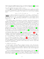

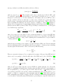
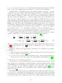
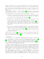


![arXiv:1306.3436v1 [hep-ph] 14 Jun 2013](http://vs1.manualzilla.com/store/data/005779061_1-09962217330e865ae44dd3cb323f6311-150x150.png)