Download Grapham User Guide

Grapham User Guide
Matti Vihola
May 24, 2013
1
Introduction
Grapham is free, experimental software. It comes without any warranty. See the
GNU General Public License [9] for details.
1.1
Objective
The main objective of Grapham is to produce numerical estimates of integrals of the
type
Z
f (x)π(x)dx
X
where f is a function of interest on the space X, which is typically Rd , but can also
have integer-valued components.1
The term “graphical model” in this setting simply means that the target density π,
or the “model,” is determined by a collection of conditional probability densities. For
example, suppose X = R3 , and that the density π is given as
π(x1 , x2 , x3 ) = cp1 (x1 )p2 (x2 | x1 )p3 (x3 | x1 ).
That is, p1 determines a probability density in R, and p1 ( · | x) and p2 ( · | x) are
conditional probability densities, i.e. specify a probability density for each x ∈ R.
Figure 1 illustrates this model. The reader unfamiliar with graphical models is advised
to take a look at some introductory material, e.g. [11, 12].
1. For such components, the integral above reduces to a sum.
1
X1
X2
X3
Figure 1: The example model “graphically.”
1.2
Algorithms
Grapham uses recently developed adaptive random-walk based Markov chain Monte
Carlo (MCMC) algorithms to produce a sequence of random variables X1 , X2 , . . . having values in the space X, such that
1 n
In := ∑ f (Xk ) →
n k=1
Z
f (x)π(x)dx =: I
X
as n → ∞. Of course, in practice, Grapham produces a finite (but long) sequence
X1 , X2, . . . , Xn , and outputs the estimate In , which hopefully approximates sufficiently
well the integral I above.
In particular, the chain is constructed by starting it at some fixed point X1 ≡ x ∈ X,
and for n ≥ 2 following the recursion
1.
simulate Yn = Xn−1 +Un , where Un are independent random vectors distributed
according to the symmetric probability density qn , and
2.
with probability αn = min{1, π(Yn )/π(Xn−1)} the proposal is accepted, and
Xn = Yn ; otherwise the proposal is rejected and Xn = Xn−1 .
If the proposal density qn in step 1 were fixed, i.e. qn = q for all n ≥ 2, this construction
would follow the well-known Metropolis algorithm.
It is a well known fact that the proposal density used in the Metropolis algorithm
determines the efficiency of the algorithm. The main purpose of the adaptive MCMC
algorithms Grapham implements is to adjust q automatically to allow efficient simulation of π. In particular, the proposal density qn above can depend on the whole
history of the chain. That is, qn (·) = qn (· | X1 , X2, . . . , Xn−1 ).
However, these proposal densities qn need to be specified with care in order to maintain the consistency, i.e. that In → I (and hence In ≈ I with large n). The algorithms
Grapham implements are described in detail in Appendix A. In particular, the implemented algorithms include
ˆ
A variant of the original Adaptive Metropolis (AM) algorithm of [10], which
uses the covariance of the whole history of the chain in the proposal. In essence,
qn (·) = fCn (·) where Cn = Cov(X1, . . . , Xn), the covariance estimate of the history, and fc is a proposal distribution with shape parameter c.
2
ˆ
Adaptive scaling random walk Metropolis algorithm of [7] and [13]. In this
case, qn (·) = fθn (·) where θn determines the scale of the proposal distribution
f . The parameter θn depends on the observed acceptance probabilities, i.e. θn =
θn (α2 , . . ., αn−1 ).
ˆ
A robust adaptive Metropolis algorithm [15], which adjusts the proposal
(pseudo-)covariance based on the directions of the proposal increments and
the observed acceptance probabilities.
It must be noted, that the theoretical validation of these adaptive MCMC algorithms is
still under serious research. Most of the algorithms Grapham implements have demonstrated to preserve correct ergodicity (i.e. that In → I), e.g. under some (restrictive)
conditions on the target distribution π. It is, however, believed that they work more
generally. The user is advised to take a look on the recent survey by Andrieu and
Thoms [6].
All the algorithms Grapham implements can be used block-wise. That is, in the context
of the above algorithm, the steps 1 and 2 are iterated m times, and each time the
(m)
variable Un has only some non-zero components. The blocks can contain freely any
components of any of the sampled variables.
1.3
Technology
Grapham is written in the C programming language2, uses some Netlib Fortran numerical routines [4], and the Lua programming language [3] in model specification.
In addition, Grapham can take advantage of the dSFMT random number generator
[5] and the Numeric Lua package [8].
The advantage of these technologies is that C and Fortran are standard technologies,
which makes it easy to compile Grapham in basically any system3 . Even though Lua
is not “standard”, it is also written in C, and also very easy to port. Moreover, these
choices allow a relatively good efficiency in the sense of simulation speed.
Other software having essentially the same purpose as Grapham include BUGS [1]
and JAGS [2]. It is not intended that Grapham competes with the existing software.
Merely, the purpose is to serve as a testbed for the recently developed adaptive MCMC
algorithms.
2
Installation
There are some binary packages of Grapham available, but it is always recommended
to use the latest source. For the binary packages, Grapham is ready for use immediately
2. More specifically, intended to be ISO C99, but may fail to comply any standards.
3. Provided that one can use IEEE double-precision floating point numbers.
3
after unpacking; see Section 3.
Before installation, make sure that you have Lua ≥ 5.1 (development package) installed. Get the latest source code of Grapham from
http://iki.fi/mvihola/grapham/. In the simplest case, the following shell
commands would compile Grapham
$ tar zxf grapham-X.Y.tar.gz
$ cd grapham
$ make
If the above fails, you must edit the file Makefile.in before issuing make. For
example, the line
LUA_PATH=$(GRAPHAM_ROOT)/lua-5.1.4
indicates that the compiled Lua package is found in the directory lua-5.1.4 under
the Grapham main directory.
If you wish to use the dSFMT Mersenne Twister random number generator (recommended), or the Numeric Lua package, you must download the source packages of
them, and edit Makefile.in to include the paths where dSFMT and/or Numeric
Lua are installed. For example,
DSFMT_PATH=$(GRAPHAM_ROOT)/dSFMT-src-2.0
NUMLUA_PATH=$(GRAPHAM_ROOT)/numlua
would work if dSFMT and Numeric Lua source packages are extracted and compiled
in the directories dSFMT-src-2.0 and numlua under the Grapham main directory.
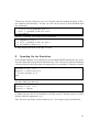
3
Running Grapham
Having downloaded and compiled Grapham, you can use it by invoking grapham under
the Grapham main directory. For example, you can simulate the Gamma distribution
by
$ ./grapham models/gamma_test.lua
Total dimension: 1 (sampling 1 with AM); With Lua calls
Results after 500000 samples (10000 burn-in):
Functional average = [ -0.005492 -0.120116 ]
Acceptance rate: 40.06%
Sampling CPU time: 1.22s (2.40us/sample; 2.40us/sample/dim)
When you have succesfully run Grapham for the first time, you can take a look inside
the file models/gamma_test.lua. The specifications in the file are explained in the
following sections.
4
The command grapham can be used with different command line arguments. The
concise usage message is shown by
$ ./grapham
(...)
Usage: ./grapham [-v|-vv|-q] [-e "lua code"] [model_file(s)]
The switch -v results in more output, and -vv even more, while -q suppresses the
output completely (excluding the functional average, if one is computed). The switch
-e can be used to provide some Lua code in the command line. If -e is issued
before the model_file argument, then the Lua code is executed before executing
model_file, and vice versa. A typical use of -e would be
$ ./grapham models/gamma_test.lua -e ’para.niter=1e6’
which runs the same test as above, but with a million iterations.
The model file(s) that are provided are Lua code that are run, when they are read.
In the example file gamma_test.lua, there are some auxiliary constants that are
computed in the first three lines
theta = 2; k = 3;
m = theta*k
m2 = (theta*k)^2+k*theta^2
These constans are visible in all what follows in the file.
For general introduction to Lua, you can read, e.g, “Programming in Lua”. The first
edition is available in http://www.lua.org/pil/. Note, however, that you do not
have to“learn”Lua completely to use Grapham. The examples provided in the directory
models provide quite many examples how things can be done.
The following sections will describe how the rest of the model specification file is built
up.
4
Model Specification
The graphical model under consideration is determined in Grapham as the table
of name model. Each of the elements of this table define one “node”, or “random
element”. The node may have a number of parents, of which the conditional density
of the variable depends on. For example, the model of Figure 1 with three nodes x1 ,
x2 , and x3 could be given as
5
model = {
x1 = {
density = function(x)
return dnorm(x,0,1)
end
},
x2 = {
parents = {"x1"},
density = function(x,x1)
return dexp(x,1+x1^2)
end
},
x3 = {
parents = {"x1"},
density = function(x,x1)
return dnorm(x,x1,0.1)
end
}
}
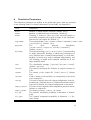
In general, the fields describing each node are as follows
Field
Description
dim
The dimension of the node; integer ≥ 1 (scalar or vector) or a
two-element table with integers ≥ 1 (a matrix).
The Lua type of the node is one of the following
"number" a scalar, which must be of dimension one.
"vector" a Lua table (of length specified by dimension.). In
the case of a matrix, a table of rows, which are tables.
"matrix" Numlua matrix class.
"custom" custom structure indexed with Lua table access
metamethods.
type
kind
parents
init_val
The kind of the node, either "real" (the default) or
"integer", in which case the feasible values of the node are
the integers.
The list of strings with the names of the parent nodes.
The initial value of the node (default: all elements zero).
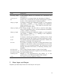
6
Field
Description
density
A function returning the logarithmic density values of the conditional probability density p(“self”|“parents”). Either a string
of the function name, or a Lua function definition. The function is called with p + 1 arguments, where the first argument
is the variable itself, and the rest are the parent variables, in
the order they appear in the field parents. Note: the value
NINF is the negative infinity, which density may return out
of its support.
A table of two elements determining the limits where the density is truncated. The first value is the lower bound and the
second the upper bound. The field can be set only with univariate distributions. The values INF and NINF are acceptable,
or alternatively nil when there is no lower or upper limit, respectively.
limits
There is a number of ready-made density functions in Grapham. The continuous,
one-dimensional densities are briefly listed below
Function
Parameters
Description
dbeta
dchi2
dcauchy
derlang
dexp
dfisher
α, β
k
x0 , γ
k, λ
b
d1 , d2
dgamma
dgumbel
k, θ
µ, β
dinvgamma
dinvchi2
dlaplace
dlevy
dlogistic
dlognorm
α, β
ν
µ, b
c
µ, s
m, v
dnorm
dpareto
m, v
xm , k
Beta distribution with shapes α > 0 and β > 0.
χ2 distribution with k > 0 degrees of freedom.
Cauchy-Lorentz with location x0 and scale γ > 0.
Erlang with shape k > 0 and rate λ > 0
Exponential with scale (inverse rate) b > 0.
F-distribution (“Fisher-Snedecor”) with d1 > 0 and
d2 > 0 degrees of freedom.
Gamma with shape k > 0 and scale θ > 0.
Gumbel (“Fisher-Tippett”), with location µ and
scale β > 0.
Inverse-gamma with shape α > 0 and scale β > 0.
Inverse-chi-squared with ν > 0 degrees of freedom.
Laplace with mean µ and scale (inverse rate) b > 0.
L´evy with scale c > 0.
Logistic with location µ and scale s > 0.
Log-normal with mean m and variance v > 0 of
log(x).
Normal with mean m and variance v > 0.
Pareto with location xm > 0 and shape k > 0.
7
Function
Parameters
Description
drayleigh
dstudent
s
ν
Rayleigh with scale s > 0.
Student’s t-distribution with ν > 0 degrees of freedom.
There is also a uniform density function duniform returning zero regardless of the
input arguments. Note that this does not determine a proper distribution.
The discrete distributions available are:
Function
Parameters
Description
dbinom
n, p
dnbinom
r, p
dpoisson
λ
Binomial with n ≥ 0 trials and success probability
0 ≤ p ≤ 1.
Negative binomial with parameters r > 0 and 0 <
p < 1.
Poisson with rate λ > 0.
The implemented multivariate distributions are:
Function
Parameters
Description
dmvnorm
µ, Σ
dmvstudent
µ, Σ, n
dwishart
V, n
Multivariate Gaussian distribution with mean µ and
covariance matrix Σ.
Multivariate t-distribution with location µ, scale Σ,
and n > 0 degrees of freedom.
Wishart distribution with positive definite scale matrix V and n > 0 degrees of freedom.
where the last, Wishart distribution is for matrices.
To see what the distributions look like, one can see, e.g., Wikipedia
http://en.wikipedia.org/wiki/Category:Probability_distributions. For
implementation details, see src/grapham_math.c.
4.1
Constants
It is possible to determine “dummy” nodes in the model, that do not have parent
variables, and have constant values. This can be done by defining a table const, of
which each element specifies a variable and the value associated to it. For example,
8
const = { a = 1, b = {2,4} }
determines two constants, real constant a and vector constant b.
The const table is actually just a shorthand notation for the definition of prior
nodes, that are instantiated with some values. Note that you do not need to define
all constants inside const. Instead, you can define any number of global variables
(and functions), and use them freely anywhere in the model. When speeding up the
simulation, however, it is necessary to define some constants inside const.
4.2
Data
The“instantiations,”i.e. the fixed values for some nodes in the model are given in the
table data. Each element of data instantiates one variable in the model to a certain
value. For example,
data = { x = {1,2}, z = 3 }
instantiate the two-dimensional vector variable x into value (1, 2)T , and the real
variable z to value 3.
4.3
Repeated Blocks
There ary many cases in which it is convenient to have“repeated blocks”in the model.
That is, a subset of the nodes in the model are duplicated, and considered as “independent repetitions”. The actual model specification of Grapham does not provide
way to “describe” this kind of model, but it provides the function repeat_block for
actually creating these repeated blocks of variables in the table model.
The function repeat_block can be called in different ways. The first argument always
contains a list of variable names that are in the block to be replicated. If the second
argument is a number N, the block is repeated N times. The other case is that the
following arguments are tables determining the values that the variables have. An
example of the latter would be
repeat_block({"y","x","z"}, {0.9, 0.7}, {0.6, 0.8})
This command would create variables y1 having value 0.9 and y2 with value 0.7.
Similarly, x1 and x2 have values 0.6 and 0.8, respectively. But the variables z1 and
z2 are left unknown.
One can also create chains of random variables, appearing most importantly in dynamic models. This is achieved by the postfix “-” after the name of the parent variable. For example, the following code creates a Markov chain (Xk )10
k=0 with X0 ≡ 0
9
and Xk+1 | Xk ∼ N(Xk , 1) for k ≥ 0 (which means that Xk is the value of a standard
Brownian motion at time k):
const = {
x0 = 0, v = 1
}
model = {
x = {
parents = {"x-", "v"},
density = "dnorm"
}
}
repeat_block({"x"},10)
This example can be found in the file models/bm.lua.
5
Functional
One can supply the functional whose expectation over the target distribution is estimated during the simulation run. In many cases, e.g. when the functional is complicated, it is more convenient to export the simulation data (see Section 7.2), and
implement the functional in some more sophisticated environment, such as R or Matlab.
The functional is defined as a global function functional, returning a lua table of
numbers (a “vector”). For example, suppose one is interested in computing the first
and second moment of the real variable x, then one could define
function functional()
return {x,x^2}
end
Alternatively, if one supplies the functional in a C library (see Section 8), then the
information of the functional is a given in a Lua table. The fields of the table are
Field
Description
name
dim
args
The name of the C function.
The dimension of the output of the function.
The arguments, i.e. the variables the functional depends on.
They are supplied as input arguments to the function, when
its value is evaluated.
10
6
Simulation Parameters
The simulation parameters are defined in the global table para, with any collection
of the following fields. For detailed information on the fields, see Appendix A.
Field
Description
niter
nburn
nthin
Number of actual MCMC iterations (default: 10e3).
Number of additional burn-in iterations (default: 0).
Thinning: if nthin>1, then only every nthin’th sample is
used when computing the ergodic average of the functional,
and saved to the output file (default: 1).
The used algorithm ["am"|"aswam"|"rbam"|"rbaswam"|"asm"|"ram"
|"metropolis"] (default: "am").
The
used
proposal
distribution
["norm"|"unif"|"laplace"|"cauchy"|"student"]
(default: "norm").
The blocking strategy ["sc"|"node"|"full"] corresponding
to “single component” blocking, in which every component of
every sampled node is sampled independently, or “node-wise”
blocking, in which every node is sampled independently, and
“full” blocking, in which all the sampled variables are in one
single sampling block.
The initialisation strategy. ["greedy"|"freeze"|"trad"]
(default: "greedy").
The name of the output file. Default: no output is written to
a file.
The format of the output file ["bin"|"ascii"] (default
bin).
A list of names of the variables (or components) to be saved
in the output file.
The name of the file where the output configuration, most importantly the (Cholesky factor of) estimated covariance matrix
is stored. By default, the output configuration is not stored.
The name of the output file where adaptation process is stored.
Default: no output file.
The format of adapt_outfile; as outfmt.
The “optimal” acceptance probability in dimension 1 (default:
0.44).
The “optimal” acceptance probability in dimension > 1 (default: 0.234).
algorithm
proposal
blocking
init
outfile
outfmt
outvars
outcfg
adapt_outfile
adapt_outfmt
acc_opt
acc_opt2
11
Field
Description
A user-defined function for performing the “acceptance rate
optimisation”.
close_hook
A function to be executed after the simulation is finished.
dr
If this is set, it determines the positive scaling factor, typically
in (0, 1), of the second phase of delayed rejection.
adapt_weight
A function returning the adaptation weight or a non-negative
real number γ (default: γ = 2/3) resulting in the adaptation
weight sequence is (n + 2)− γ. This weight is used when computing the covariance factor.
adapt_weight_sc Like adapt_weight, but this value is used for scale adaptation with algorithms with a coerced acceptance probability
("asm"|"aswam"|"rbaswam")
adapt_weight
A function returning the adaptation weight, or a non-negative
real number γ (default: γ = 1) resulting in the adaptation
weight sequence is (n + 2)−γ.
p_mix
A function returning the probability of drawing from a fixed
proposal component. By default, not fixed component is used.
seed
The random seed of the pseudorandom generator. Default: the
generator is initialised from system time.
blocks
The blocks of variables, as a table of tables with names of the
variables in each block. If this is not specified (or not all the
variables are in the specified blocks), the selected blocking
strategy determines the blocks (of remaining variables) automatically.
blocks_chol
List of initial Cholesky factors of each of the blocks.
blocks_chol_sc An extra scaling factor that is applied to the Cholesky factors.
blocks_scaling The initial scaling factor.
random_scan
Whether to use systematic-scan (the default, 0), or the
random-scan (6= 0) Metropolis-within Gibbs sampler.
clib
The name of the user-supplied C library.
scaling_adapt
7
Data Input and Output
Grapham provides simple means for data import and export.
12
7.1
Importing Data
In many cases, one has a set of data in some format, that needs to be “applied” to a
model in Grapham. If there are few data points, it may be sufficient to directly define
them in the model specification. However, if there are very many data points, it is
useful to be able to import the data automatically. Grapham provides only one way
to import data: by the means of CSV (comma separated values) ASCII files.
A typical example would be the following
vars, y_data = read_csv("data.csv")
repeat_block(vars, unpack(y_data))
In this case, the data is read from the CSV file data.csv. If there is a “header line”
in the file, consisting of the names of the variables, they are stored in the Lua table
vars (otherwise, vars is empty). The data is read into y_data, where y_data[i]
is the i:th column of the CSV file. The Lua function unpack makes them separate
arguments to the function repeat_block.
Although Grapham does provide only CSV importing, it is possible to write input
routines for any kind of data, since Lua is a full-featured programming language, and
provides I/O routines in the io module.
7.2
Exporting Data
In some situations, it may be insufficient only to have the average of some functional
of the samples. It may be more convenient to store a whole set of simulated samples,
and work in some other environment. Grapham provides two output file formats: CSV
and binary. The CSV format is standard, and read by many programs, but it has
the downside that the files tend to be unnecessarily large that are slow to write by
Grapham, and slow to read by any other program.
The binary file format of Grapham produces small files that are essentially just“dump”
of the data. They are fast to write and read to another program. The files consist of
the header line, which is identical to that of the CSV file. The rest of the file is just
raw dump of the binary double-precision floating point numbers.
The data can be exported from Grapham by means of two parameters para.outfile
and para.outftm described in Section 6. There are input routines ready for the (free)
GNU R, and (proprietary) Mathworks Matlab. The tools can be found in the directory
tools.
As an example, run Grapham with the model file example.lua.
$ ./grapham models/example.lua
13
This writes a binary output file out.bin. Suppose that the working directory of R is
the Grapham main directory. The file out.bin can be read to R and visualised with
the commands
> source("tools/grapham_read.r")
> data <- grapham_read("out.bin")
> plot(data)
Similarly, in Matlab, one could use the commands
>> addpath(’tools’)
>> data = grapham_read(’out.bin’)
>> plot(data.z,data.x_2_,’.’)
to read and plot the data in the file out.bin.
8
Speeding Up the Simulation
Even though Grapham is not intended to be the fastest MCMC simulation tool, there
are some ways that may speed the simulation up a bit. First of all, instead of defining
a density function that just passes the arguments to a predefined C-function, such as
...
parents = {"m", "v"},
density = function(x,m,v)
return dnorm(x,m,v)
end
...
one may define the above as
...
parents = {"m", "v"},
density = "dnorm"
...
in which case one call of Lua function is avoided, as the C-function dnorm is called
directly with the arguments x,m,v.
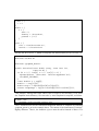
Also, the user may define custom densities in C. An example model specification:
14
const = {
c = 5
}
model = {
x = {
dim = 2,
density = "dcircular",
parents = {"c"}
}
}
para = {
clib = "clib/dcircular.so",
outfile = "circular.bin"
}
and the file dcircular.c, which is compiled into shared library file dcircular.so:
#include <stdio.h>
#include <stdlib.h>
#include "grapham_math.h"
double dcircular(const double **arg, const int* len,
const int N) {
if (N != 2 || len[0] != 2 || len[1] != 1) {
fprintf(stderr, "dcircular: Invalid arguments.\n");
exit(EXIT_FAILURE);
}
const double* x = arg[0];
double c = arg[1][0];
double nsqx = c-sqrt(x[0]*x[0]+x[1]*x[1]);
return -nsqx*nsqx + log((1+cos(5*x[0]))*(1+cos(5*x[1])));
}
This example, among with some others, can be found in the directory clib under
the Grapham main directory. One can test it, once Grapham is compiled, as follows
$ make clib
$ ./grapham clib/circular_target.lua
The C functions can use the standard distributions defined in Grapham by including
grapham_math.h, as in the example above. The names of the functions are, however,
slightly different. That is, the function d_beta must be called instead of dbeta. For
15
more information, the function prototypes with brief explanation can be found in the
file grapham_math.h.
References
[1]
[2]
[3]
[4]
[5]
[6]
[7]
[8]
[9]
[10]
[11]
[12]
[13]
[14]
[15]
A
The BUGS project. URL http://www.mrc-bsu.cam.ac.uk/bugs/.
JAGS just another Gibbs sampler. URL http://calvin.iarc.fr/~martyn/software/jags/.
The programming language Lua. URL http://www.lua.org/.
Netlib repository. URL http://netlib.org/.
SIMD-oriented fast Mersenne twister. URL http://www.math.sci.hiroshima-u.ac.jp/~m-mat/MT/SFM
C. Andrieu and J. Thoms. A tutorial on adaptive MCMC. Statist. Comput., 18(4):
343–373, Dec. 2008.
Y. F. Atchad´e and J. S. Rosenthal. On adaptive Markov chain Monte Carlo algorithms.
Bernoulli, 11(5):815–828, 2005.
L.
Carvalho.
Numeric
Lua
project
page,
2005.
URL
http://luaforge.net/projects/numlua/. Visited 11th June 2009.
Free Software Foundation. GNU general public license, version 3, June 2007. URL
http://www.gnu.org/licenses/gpl-3.0-standalone.html.
H. Haario, E. Saksman, and J. Tamminen. An adaptive Metropolis algorithm.
Bernoulli, 7(2):223–242, 2001.
F. V. Jensen. Bayesian Networks and Decision Graphs. Springer-Verlag, New York,
2001. ISBN 0-387-95259-4.
K. P. Murphy.
Dynamic Bayesian Networks: Representation, Inference and
Learning.
PhD thesis, University of California, Berkeley, 2002.
URL
http://www.ai.mit.edu/~murphyk/mypapers.html.
G. O. Roberts and J. S. Rosenthal. Coupling and ergodicity of adaptive Markov chain
Monte Carlo algorithms. J. Appl. Probab., 44(2):458–475, 2007.
G. O. Roberts and J. S. Rosenthal. Examples of adaptive MCMC. J. Comput. Graph.
Statist., 18(2):349–367, 2009.
M. Vihola. Robust adaptive Metropolis algorithm with coerced acceptance rate.
Statist. Comput., 22(5):997–1008, 2012.
The Algorithms
The general form of the implemented algorithms, as well as several adjustable parameters, are described in Section A.1. The different initialisation strategies are described
in Section A.2.
If several sampling blocks are used, a “sweep update” is performed, i.e. they are
updated sequentially and the algorithms described below are applied to each of the
blocks separately. The order in which the blocks are updated is static, and does not
change from iteration to another.
16
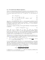
A.1 The Implemented Adaptive Algorithms
All but one of the algorithms implemented in Grapham can be summarised as follows.
Let X1 ≡ x1 ∈ Rd be an initial point (by default, a zero vector), and let S1 ≡ s1 > 0
be a positive definite matrix, and Θ1 ≡ θ1 > 0. Define M1 := X1 , and recursively for
n≥1
Xn+1
Mn+1
Sn+1
Θn+1
∼
=
=
=
PΘn Sn (Xn , ·)
(1 − ηn+1 )Mn + ηn+1 Xn+1
(1 − ηn+1 )Sn + ηn+1 (Xn+1 − Mn )(Xn+1 − Mn )T
hn+1 (Θn , αn+1 )
(1)
(2)
(3)
(4)
where PS (x, ·) is the MCMC kernel, and αn+1 is the acceptance probability from the
MCMC kernel. The adaptation weights ηn are by default n−1 , and can be determined
by defining a function para.adapt_weight, that receives k ≥ 0 as the argument,
and returns the value of 0 ≤ ηk+2 < 1.
The function hn adapts the scaling of the proposal distribution. The default function
is defined as
(sc)
(5)
hn (θ, α) := θ exp ηn (α − αopt )
(sc)
can be defined like ηn above, but using the parameter
where ηn
para.adapt_weight_sc. where αopt is the target acceptance probability, defined
by para.acc_opt1 and para.acc_opt2. One can define a custom hn by definining
the function para.scaling_adapt. The initial value of the scaling parameter θ1 is
by default 2.382/d, and the default value of s1 is the identity matrix.
The kernel Ps (x, ·) is a Metropolis kernel with a symmetric proposal distribution (see
Section A.3) having covariance s. A sample Z from Ps (x, ·) can be simulated as follows
1.
Draw a proposal random variable Y from q(·; x, s).
n
o
)
2.
Let Z := Y (“accept”) with probability α = α(x,Y ) := min 1, π(Y
, and let
π(x)
Z := x (“reject”) with probability 1 − α.
If one uses delayed rejection, then Ps (x, ·) is a kernel determined by a two-phase
algorithm. The first phase is as described above, but if the first proposal Y is rejected,
then another independent proposal Y2 is generated, from the a Gaussian distribution
with mean x and covariance ρs, where ρ > 0 (typically 0 < ρ < 1) is the parameter
para.dr. This second proposal is accepted with probability
π(Y2 )q(Y2 ;Y, s)[1 − α(Y,Y2 )]
min 1,
.
π(x)q(Y2; x, s)[1 − α(X ,Y2)]
in which case Z := Y2 , and otherwise Z := x. (Note: the acceptance probability that
is used by hn is the one from the first proposal.)
17
The algorithm para.algorithm="aswam" (“adaptive scaling within AM”) implements all (1)–(4). In the case of AM, i.e. para.algorithm="am", the
scaling is not adapted, i.e. hn (θ, α) ≡ θ. The option para.algorithm="asm"
(“Adaptive scaling Metropolis”) implements only (1) and (4), while the choice
para.algorithm="metropolis", i.e. a standard non-adaptive Metropolis algorithm
implementing only (1).
The “Rao-Blackwellised” versions of AM, para.algorithm="rbam" and
para.algorithm="rbaswam", correspond to para.algorithm="am" and
para.algorithm="ams", respectively. They implement instead of (2) and (3)
the following recursions
Mn+1 = (1 − ηn+1 )Mn + ηn+1 [α(Xn ,Yn+1 )Yn+1 + (1 − α(Xn ,Yn+1 ))Xn]
Sn+1 = (1 − ηn+1 )Sn + ηn+1 α(Xn,Yn+1 )(Yn+1 − Mn )(Yn+1 − Mn )T
+(1 − α(Xn,Yn+1 ))(Xn − Mn )(Xn − Mn )T
(6)
(7)
where Yn+1 is the proposed value in the n + 1:th step. See [6] for derivation.
The robust adaptive Metropolis, para.algorithm="ram" implements does not update the scaling separately, but instead of (3), the covariance factor Sn is updated
according to the rule
UnUnT
1/2
1/2
(Sn )T
I + ηn+1 (αn+1 − αopt )
Sn+1 = Sn
kUnk2
1/2
where Un = Sn (Yn+1 − Xn ) is the normalised proposal increment; see [15] for details.
A.2 The Initialisation Strategies
There are three initialisation strategies available, which can be specified in para.init.
The default strategy, "greedy", stands for continuous adaptation, that is performed
both during burn-in and estimation. That is, (1)–(4) are applied all the time. The safe
option "freeze" means that adaptation is “frozen” after burn-in, and the estimation
is performed with standard Metropolis kernel. This means that for n > nburn-in , only
the equation (1) is applied. The option "trad" means an adaptation in the spirit of
the seminal paper [10]. This means that for n ≤ nburn-in, (1) is replaced with
Xn+1 ∼ PΘ1 S1 (Xn , ·)
(8)
When n > nburn-in, then (1) applies.
It is also possible to determine a proposal density that is a mixture of two proposal
densities. That is, (1) is replaced with
Xn+1 ∼ pn+1 PΘ1 S1 (Xn, ·) + (1 − pn+1 )PΘn Sn (Xn, ·)
(9)
18
where 0 ≤ pn+1 ≤ 1 is the probability of drawing from the initial proposal density.
This is achieved by the field para.p_mix, which is a function that receives k ≥ 0
as an argument and returns 0 ≤ pk+2 ≤ 1. If this function returns a a “small” fixed
value, this reflects to the modification proposed by [14]. By determining a sequence of
probabilities 1 = p2 > p3 > · · · pk → 0, one can have in a sense a“gradual”initialisation,
since (9) is the same as (8) for n = 1, and “(9) → (1)” as n → ∞.
A.3 The Proposal Densities
There are different proposal densities that can be used in Grapham. All the proposals
use a sim´ılar generation procedure: Y = X + LU , where X is the current position, L
is the Cholesky factor of the covariance matrix, and U is a zero-mean, symmetrically
distributed random variable with unit variance.
In fact, all but one of the implemented proposal distributions define U = (U1 , . . .,Ud ) ∈
Rd as a vector of independent and identically distributed Ui . The possible distributions
for the distributions of Ui , determined by para.proposal, are
ˆ
ˆ
ˆ
"norm" Gaussian N(0, 1) (this is the default).
√ √
"unif" Uniform distribution in interval ( 3, 3).
"laplace"
√ Laplace (or “two-tailed exponential”) distribution with zero mean
and scale 2.
In addition, the choice "student" determines a multivariate Student distribution
(with one degree of freedom). That is, the vector U has the density f (x) = c(1 +
xT x)−(d+1)/2 where c > 0 is a constant.
Observe that only the options "norm" and "student" determine a spherically symmetric distribution for U .
19