1
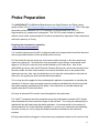
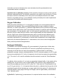
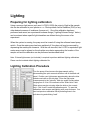
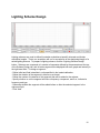
Algae Light and Gas Instruments (ALGI) Dissolved Gas Analyzer 1.0 (DGALPT 1.0) User Manual Revision 3.0 August 2013 ALGI, LLC 6606 South Chase Court Littleton, Colorado 80123 contact: ALGInstruments.com Hardware: ed@algI.com Software: devin@algI.com Experimental Design/Biology: jon@algI.com 1 Preface: Software Installation and Instrument Setup Software Installation Other required hardware (calibration gas purging systems) Filling the fluid temperature control system Instrument Start up Probe Preparation Probe Polarization and Calibration Oxygen Calibration Hydrogen Calibration Probe storage and maintenance Lighting Preparing for lighting calibration Lighting Calibration Procedure Lighting Scheme Design LED temperature control Sample Temperature Control Experimental Parameters Acquisition Procedure Experimental data file naming and storage Starting an Acquisition Experimental Parameters Data Analysis Panel Data Export Troubleshooting References and Patents 2 Preface: Software Installation and Instrument Setup Software Installation The required software is provided on a USB flashdrive. Updates can be provided from ALGI, LLC by mail on a DVD disc. Contact us through our website for a direct link to download the software directly from the web. Our software requires additional drivers which are installed using the provided installer. Simply transfer the provided folder to the appropriate place for programs on your computer’s harddrive and click on the installer’ setup file within the folder. Other required hardware (calibration gas purging systems) For H2 measurements, a calibration gas cylinder (5% recommended), appropriate regulators, a purging station, and purging needles capable of bubbling gases into the sample cell are required. Similarly, H2 baseline data can be acquired by purging the measured gas completely out of solution by bubbling with an inert gas (Argon or Nitrogen). The O2 consuming reducing agent, sodium dithionite (i.e. sodium hydrosulfite) is also sometimes used to for the baseline measurement for O2 measurements, however, this reagent does not typically have a long shelf life and is prone to partial oxidation over time. Therefore, for greatest reproducibility, we recommending taking “Low” O2 baseline measurements with the probes polarization set to “0”. Filling the fluid temperature control system “On Newer systems that include an ALGi logo on the front panel, please use the following youtube video link to see demonstration videos of how to correctly fill the system ” http://www.youtube.com/user/alginstruments?feature=results_main If your system arrives “dry”, the waterjacket system will need to be filled. To do this, remove the lid using a phillips head screwdriver to remove the four retaining screws. 3 Inside, an orange Tfitting can be located. This fitting has a quickconnect containing an orange plug that can removed by hand. The provided external hose can be pressed into this fitting temporarily for filling. The second provided hose, attached to a “male” metal quickconnect fitting, can be pressed into the drain on the backright hand corner of the system. Once the two hoses are connected, a deionized water source can used to flow water through the entire system. The user may need to hold the system at various angles to help allow the escape of entrapped air as the water flows through the circuit. Once it seems that all the air has been removed, both hoses can be removed, and two drops of the provided “Bioguard” solution preventing growth within the water system can be added to the water before reapplying the orange plug and reaffixing the lid and retaining screws. Instrument Start up 1. To begin communication of the system to the computer, plug in the provided USB cable connecting the internal National Instruments DAQ6009 to the computer. The green indicator light on the instrument blinks when communication has been established. 2. Open the ALGI_app software. On the main window the left most pane should indicate the name of the USB6009OEM data acquisition card (DAQ) in communication with the computer. Click “Open ACQ.” 3. Once the software has been started and communication to the DAQ has been established, the primary power supply switch may be turned on. All primary power, except for probe polarization, including stirring, lighting & sample temperature control, are powered by the power supply box. The power supply should be plugged into a grounded 100264V AC power outlet. The power supply has a single plug used to connect to the main instrument. When this plug is connected to the main instrument care must be taken to line up the plug properly and it can then be turned clockwise to firmly connect all sources of power. The provided stir plate also has an independent on/off switch. When the stir plate is turned on, a green indicator LED on the surface of the stir plate can be seen illuminated. 4 Important note: There is a switch on the stir plate that initiates alternating stirring. Care must be taken that this switch is always off so that stirring is consistent. Important notes: When the main power switch is turned on, the user must confirm the cooling fans on the white power supply box are running and not blocked or power supply failure due to overheating is likely. Also, if the primary power supply is turned on when there is no communication to the ALGI software, the LED light may turn on full brightness without any temperature control, and damage to the LED by overheating could occur. To maintain the longevity of the LED, it is important to establish communication to the software prior to turning on the main power supply switch. 5 Probe Preparation The ALGIDGALPT 1.0 (Dissolved Gas Analyzer with Light, Pressure and Temp control) system utilizes YSI (http://www.ysireagents.com/category.php?categoryId=328) 5331 Clarktype electrodes and the associated YSI 5775 Standard (O2 measurement) and YSI 5776 Highsensitivity (H2 measurment) membranes. The YSI 5331 probe consists of a platinum cathode, silver anode, and saturated KCL solution contained by a disposable Teflon® membrane and held in place by an Oring. Preparing the electrodes for operation: video of electrode preparation 1. If a new kit is being used, the KCL crystals provided in the dropper bottle should be dissolved with enough distilled water to fill the provided bottle to the top. 2. If the electrode has been previously used, tarnish which develops on the silver anode may need to be cleaned off. One method to clean the probe involves using a cottontipped swab dipped in 3% NH4OH to wipe the silver anode followed by a DI water rinse. Also, a fine (40008000 grit) emory cloth (ALGI Electrode Cleaning Kit) may be used to remove tarnish from the silver anode, but care must be taken to not remove excessive silver or the probe will be destroyed over time. Also, care should be taken not to clean the center platinum electrode too often since it is typically the silver side that becomes oxidized. 3. An oring should be applied to the provided plastic applicator in preparation for installing the membrane. If this is a newly purchased system a membrane installation kit should be included that makes installing membranes a little easier. There should be an included manual that explains how this kit should be utilized. 4. A drop of saturated KCL solution should be applied to the probe head. 5. A Teflon® membrane should be stretched across the probe head to entrap the KCL droplet and held affixed with thumb and index fingers of the left hand. The oring can subsequently be applied with the right hand using the plastic applicator. It is recommended for the majority of measurements to use a high sensitivity membrane. If you find your experiments are saturating the probe circuits you can try using the standard sensitivity membranes, both should be included. 6. Each probe should be plugged in to the phono plug receptacles located on the rearleft of the 6 instrument and polarized for a minimum of 30 minutes such that probe baselines and responses stabilize prior to calibration using standard gas concentrations. 7. The probes can now be gently pressed into the glass cell such that the orings seal at the designed constriction points. Care must be taken that Teflon® membrane is not excessively folded or bunched as to cause pressure on the walls of the cell, or breakage could occur. Once the two probes are installed, the provided 3 x 3 mm stir bar (Wilmad Labglass (LG9566T108)), desired 1mL liquid solution, and capillary airlock can be added to complete the initial set up. 7 Probe Polarization and Calibration After finalizing the initial set up of the electrodes and glass cell, set the appropriate polarization voltage based on the type of measurements desired. The software should automatically set the appropropriate polarization voltage based on the mode you select. The system is designed so either electrode may be used for O2 or H2 measurement, in the event the polarization voltages are not correct, these are the suggested settings for polarization: O2 polarization: 0.8 V H2 polarization: + 0.6 V low O2 baseline Probe Baseline Panel “Probe ID” names can be manually entered so that calibration values can be stored. This is helpful for two reasons. First, in case of software failure the probe calibration can be reloaded with ease. Second, saving calibration data allows the user to track the sensitivity of the 8 electrodes over time to determine when new electrodes should be purchased due to an unreasonable decline in sensitivity. Important note on calibration accuracy: Probe sensitivity changes over time as the Ag anode becomes coated with tarnish. The decline in sensitivity is very great in the first 30min to 1h, then the slope of decline is reasonably low for many hours as the response become more stable. However, for greatest accuracy, a new calibration can be performed prior to each experimental measurement by bubbling with calibration gases. Oxygen Calibration Setting the probe polarization to “0” or unplugging the probes is our recommended method to determine the low baseline. Other users prefer purging with inert gas or addition of sodium dithionite (i.e. sodium hydrosulfite). O2 calibration (High baseline) can be performed simply using the same solution which will be used in the subsequent assays in equilibrium with atmospheric gas concentration. For high baseline, add 1 mL of the same airsaturated solution,, ensure that the micro stir bar is freely stirring in solution, wait for signal stability and temp equilibration, and click the “High” button under the appropriate probe menu to record the high calibration point. Onboard barometric pressure sensor and userdefined salinity values input into the software are used to calculate the O2 concentration in solution which corresponds to the voltage signal produced by the electrode polarized for O2 measurement, so be sure to have the appropriate salinity values input before taking baselines. Hydrogen Calibration H2 calibration can be performed using a 5% (recommended) H2:Ar gas mixture. Unlike other Clark electrode systems, the ALGIDGALPT has built in amplification and filtering for the H2 measuring circuit that does not require the preparation of “platinum black” by alternating polarization overnight. Instead, a polished platinum YSI 5331 electrode response to a 5% H2 gas mixture when polarized at 0.6 V on the H2responsive circuit should correspond to approximately 23 V. The exact % of H2 used for calibration should be entered in under the “Probe Baselines” tab. To calibrate, infuse a solution of 1 mL water or appropriate biological buffer in the sample cell by bubbling with the gas mixture, wait for signal stability, and record the “High” calibration point. Insert the percentage gas mixture into the “H2 Gas Cal %” field under the “Probe Baselines” tab (e.g. 5% H2 gas mixture = 5). It is important when doing the H2 calibration that the gas line is first completely purged with the standard gas or proper signal will not be reached. To determine the electrode baseline, simply purge with Argon or Nitrogen, wait for signal stability, and record the “Low” calibration point. H2 Gas Cal %: If performing H2 measurements, it is required that the mixture of the calibration 9 gas, in % composition, be entered into this window of the “Probe Baseline” tab. The provider of the calibration gas should provide a spec sheet with this data attached to the provided gas tank. This value is used by the software to determine the appropriate molar concentration represented by the voltage difference recorded during high and low calibration data acquisitions. Probe storage and maintenance The probes are a consumable component of the ALGIDGALPT system, but their lifetime can be extended by proper care. Electrodes should only be polarized when active measurements are being performed to extend their lifetime. If the probes are left polarized for extended periods, their sensitivity will be markedly reduced. Sensitivity can be restored by cleaning tarnish from the silver anode, however, after multiple cleanings the silver itself will be removed and the probe will no longer function. When not in use, the probes should be stored dry, covered with a membrane, unpolarized, and unplugged. 10 Lighting Preparing for lighting calibration Using a common light sensor such as a LICOR LI250A the output of light at the sample site can be calibrated to µmol photon m2 s1 Photosynthetic Active Radiation (PAR) or any other desired measure of irradiance (lumens ect.). Once this calibration has been performed and saved, an experimental scheme design (“Lighting Scheme Design” button) can be entered where specific light intensities are defined during the course of an experiment. When the system is running, the pump must be turned off using the softwarebased pump switch. Once the water pump has been switched off, the glass cell may be removed by depressing the metal quickconnects. With the cell removed, the LICOR or equivalent light meter sensor can be placed on the stirplate cross hairs representing the location of the sample cell and the calibration can be performed as described below. Note: External light sensor (not included) is required to perform additional lighting calibrations. Please use the included default lighting calibration file. Lighting Calibration Procedure Turn the pump off and remove the glass sample cell by disconnecting the quick connects at either end of the black mid panel. Position your light sensor approximately above the blue dotted cross hairs on the stir plate. Enter the light meter measurements in the “Intensity” field at a series of slide values ranging from 010 at 0.5 increments of the “Slide Value” field. Slide values may be set using either the slide or the numeric field. Click “Insert” to add the calibration point. To save this calibration, enter a name and lighting units, and click save. You can load previous calibration files by selecting them in the pulldown ring and clicking “load”. 11 Lighting Scheme Design Lighting schemes are used to define illumination schedules at specific intervals and dictate acquisition lengths. That is, an acquisition will run for a maximum of the designated length of a saved lighting scheme. To prepare a lighting scheme, click the “Lighting Scheme Design” button. Schemes are composed of a number of segments defined by the parameters at the top of the Scheme Design tab, and all active segments are displayed both as a graph and textually in the rightmost field. To design a segment: Define initial and final intensities in units specified in the loaded calibration, Define the duration of the segment in hh:mm:ss.ss format, Define the number of instances of this segment that will be added to the scheme, Specify whether or not the segment will have a frequency component, and if so, indicate its frequency and type, Determine whether the segment will be added before or after the selected segment in the rightmost field, Click “Add” 12 A 15 second 0100 ramped 3 Hz square wave with segment multiplier of 3. A composite lighting scheme. The segment selected in the right field is bounded by the red cursors in the graph. Prior to inserting a segment into a scheme, a single instance of the segment is previewed in the small upper graph (F). The segment will be, by default, inserted after whichever segment is selected in the list. By selecting a segment in the segment list, the new segment may be inserted either before or after the selected segment by toggling the “Before After” switch. Segments, or combinations of segments (selected using Ctrl+ or Shift+ left click), can be copied 13 or deleted using the controls at the bottom of the segment list (H). As well, schemes can be cleared by clicking the “Clear” button. Schemes can be saved and loaded for editing later by typing a name in the upperright most field and clicking “Save” or by selecting a scheme in the pulldown menu and clicking “Load.” (G) LED temperature control In the early stages of our research and development, we found that the intensity of the LED output would drop off significantly as the LED heated up during an experiment. Thus, without maintaining a constant temperature, we could not calibrate and define a specific photonic flux with confidence. The current system features an LED illumination system kept at 30 ºC by a digitallycontrolled peltier thermoelectric temperature management system. This system is capable of maintaining the LED at constant temperature well above the equivalent of full solar incidence (2500 µmol photon m2 s1 PAR). However, the lighting can be driven up to approximately 8000 µmol photon m2 s1 PAR, which is above the point that the peltier system can maintain constant temperature for long periods. Thus, the ALGI software incorporates an indicator light which provides a visual reference that constant temperature of the LED is maintained. When the “LED @ Temp” indicator is not highlighted, the user is informed that proper temp, and thus maintenance of calibrated LED output, cannot be assured. Moreover, if the LED is driven at high intensities for periods longer than constant temperature is maintained, the LED lifetime and consistency of photonic output cannot be assured. Thus, we recommend lighting intensities and schedules that keep the indicator light highlighted. Lighting Spectrum of Photosynthetic Active Radiation (PAR) at 400700nm. 14 Sample Temperature Control Temperature can affect the response of the electrodes, the molarity of dissolved calibration gases, and the behavior of a biological sample. For these reasons, it is important to define a constant temperature setting for each experiment. To set the temperature desired for an experiment, the user can refer to the top of the main “Acquisition” panel. The actual temperature is displayed both as a red line on the graph and as a number in the Temp (ºC) window. The “set point” can be easily adjusted by the user by either dragging the thermometer display to the desired temperature, or simply inputting the precise temp (ºC) in the window above the the thermometer display. Temperature Calibration 15 Experimental Parameters Cell counts: Concentration of cells can be determined by hemocytometer or Coulter principlebased particle counters like the Z™ Series COULTER COUNTER® Cell and Particle Counter. In the “Acquisition” panel under “Experiment Data” cell count data ( x 103) can be entered prior to an experimental acquisition and this data will be saved for downstream analysis. Cell count data can also be used for data analysis after an experimental run but entering the appropriate data in the “Analysis” panel and hitting “Reprocess”. 16 Chlorophyll: Total chlorophyll (Chl) concentrations from algae or cyanobacteria cultures is typically determined by solvent extraction (ethanol or methanol), cell debris removal by centrifugation, and spectrophotometric determination. The experimentally determined µg Chl equivalents in the algae sample assayed can be entered into the “Experiment Data” section prior to analysis and will be stored as meta data for downstream analysis. Similar to cell count data, Chl data may also be entered in manually during data analysis with data appropriately recalculated using the “Reprocess” button in the data analysis section. Salinity: For measurements done in solutions which have low salinity, this value can be left set to zero. However, if measurements are done in solutions of high salinity (ocean water or greater), then it is appropriate to provide a salinity value (ppt) so that the differences in dissolved calibration gases compared to fresh water can be accounted for. Also, despite providing a salinity value for appropriate calculation of dissolved gases, care also must be taken in consideration of the greater sensitivity of the electrodes in solutions of greater salinity because of the higher fugacity of the dissolved gases. In other words, the dissolved gases will be driven into the KCL electrolyte to a higher degree when the sample solution is high in solutes. To properly account for the salinity affect on the electrode sensitivity, simply be sure to do all gas calibrations in a buffer of the same ionic composition as the sample to be assayed. Volume: This parameter should not need to be changed. The sample cell volume accommodates 1 mL of solution. Barometric pressure: Atmospheric pressure (atm) is recorded by an onboard integrated circuit pressure sensor. The value being acquired from this circuit is displayed in the software “Acquisition” panel adjacent to the temperature data. This value is used to determine the precise molar concentration of calibration gases based on welldefined values at varying partial pressures. Simply put, the molar concentration of dissolved oxygen in solution is directly proportional to the atm. So a solution saturated with atmospheric oxygen in Golden, CO (at approximately 0.83 atm) will contain 83% of the moles of oxygen of the same solution at sea level. The software takes this into account, and when high and low calibration baselines are acquired, appropriately defines that differences in voltage as equivalent to the appropriate molar quantity of gas in solution. 17 18 Acquisition Procedure Experimental data file naming and storage Prior to running an experiment meta data which will control how the data is stored must be entered in under the “File Info” tab of the “Acquisition” panel. Data folders are stored in a folder labelled “Data” within the ALGI software folder. The “User Name” field will define the name of the folder which your data will be stored under, in addition to a subfolder based on the date of acquisition. Similarly, the “Acquisition Name” field will determine the name of the file which is being acquired. This field is completely flexible as to the format which the scientist is most comfortable with storing their data. If subfolders are desired for storing data, for instance in cases where the same user would like to do experiments for different projects on the same day, we have provided the “Data Set Name” field, which will define subfolders for storing data. The comments field also allows the scientist to store additional notes, as desired, within the stored data file as meta data. 19 Starting an Acquisition To start an acquisition, the user simply clicks the “Start Acquisition” button visible on the main panel. When this button is depressed, the current probe baselines, experimental data, file info, temp set point and lighting scheme design information is all referenced to inform the experiment as designed by the experimentalist. The blue indicator bar adjacent to the “Start ACQ” button can allow the progress of the experiment to be visualized. 20 Experimental Parameters Cell counts: Concentration of cells can be determined by hemocytometer or Coulter principlebased particle counters like the Z™ Series COULTER COUNTER® Cell and Particle Counter. In the “Acquisition” panel under “Sample Data” cell count data ( x 103) can be entered prior to an experimental acquisition and this data will be saved for downstream analysis. Cell count data can also be used for data analysis after an experimental run but entering the appropriate data in the “Analysis” panel and hitting “Reprocess”. Chlorophyll: Total chlorophyll (Chl) concentrations from algae or cyanobacteria cultures is typically determined by solvent extraction (ethanol or methanol), cell debris removal by centrifugation, and spectrophotometric determination. The experimentally determined µg Chl equivalents in the algae sample assayed can be entered into the “Experiment Data” section prior to analysis and will be stored as meta data for downstream analysis. Similar to cell count data, Chl data may also be entered in manually during data analysis with data appropriately recalculated using the “Reprocess” button in the data analysis section. Barometric pressure: Atmospheric pressure (atm) is recorded by an onboard integrated circuit pressure sensor. The value being acquired from this circuit is displayed in the software “Acquisition” panel adjacent to the temperature data. This value is used to determine the precise molar concentration of calibration gases based on welldefined values at varying partial pressures. Simply put, the molar concentration of dissolved oxygen in solution is directly proportional to the atm. So a solution saturated with atmospheric oxygen in Golden, CO (at approximately 0.83 atm) will contain 83% of the moles of oxygen of the same solution at sea level. The software takes this into account, and when high and low calibration baselines are acquired, appropriately defines that differences in voltage as equivalent to the appropriate molar quantity of gas in solution. 21 Salinity: For measurements done in solutions which have low salinity, this value can be left set to zero. However, if measurements are done in solutions of high salinity (ocean water or greater), then it is appropriate to provide a salinity value (ppt) so that the differences in dissolved calibration gases compared to fresh water can be accounted for. Also, despite providing a salinity value for appropriate calculation of dissolved gases, care also must be taken in consideration of the greater sensitivity of the electrodes in solutions of greater salinity because of the higher fugacity of the dissolved gases. In other words, the dissolved gases will be driven into the KCL electrolyte to a higher degree when the sample solution is high in solutes. To properly account for the salinity affect on the electrode sensitivity, simply be sure to do all gas calibrations in a buffer of the same ionic composition as the sample to be assayed. Data Analysis Panel To view acquired data, click on the “Analysis” tab at the top of the window. In the upperleft most field, click the folder icon to open the acquisition folder. Navigate to the desired file, and click OK. The experiment and sample information will be loaded into the fields “Cell Count,” “Chlorophyll,” “H2 Gas Cal %,” and “Salinity” and the acquired data will be displayed in the bottom graph. The experiment and sample information can be changed and will automatically update on the graph (as will changing any field on the analysis panel), but the new value will not be saved to disk until the file is right clicked and “Save” is selected. 22 Similar to the acquisition panel, the units of the loaded data can be changed by selecting the desired units format through the top buttons in the “Units Select” section. The selected units will appear as a label on the lefthand yaxis, while the lighting units will appear on the righthand yaxis. Selecting “Voltage” will disable any other unit selection, and report unscaled voltage. Acquisition data can be filtered and smoothed using both the lowpass filter frequency and the smoothing slide. On each graph are cursors that report yvalues of data sets. By default, these cursors are associated with the first data set (Probe 1). 23 Data Export Data can be exported from either the “Acquisition” or “Analysis” panels by pressing “Export” or right clicking the graph and selecting “Export.” Data presented in each respective graph will be captured and displayed on the export panel as both an image and collected data arrays. The units and filtering of original data are preserved in the exported data. For example, if the loaded data is presented in ‘umole,’ the exported data will be of ‘umole.’ Each data array’s name is shown to its left. To save the image and data, select the image format and press “Save”. All numeric data is saved to a *.csv excel file with the file path indicated in the field at. To export only unprocessed, unfiltered voltage data, make sure that, in the “Analysis” window, that “Lowpass Filter” is set to >50, smoothing is set to 0, and that “Voltage Only” is marked in the Units Select section. Then, select the “Concentration” tab and ensure the desired data sets are selected in the legend. Select “Export” and in the export panel, press “Save.” This will save raw voltage data acquired from the probes without baseline scaling or processing. Troubleshooting Despite our best effort to design a robust, userfriendly system, Clark electrodebased measurements of biological gas exchange are still an art. We have done our best to design a system which controls many of the confounding variables which may cause experimental inaccuracies. However, problems with the probe chemistry/teflon membrane are the most common cause of system malfunction. For instance, if sample solution gets around the oring and makes contact with the Ag anode, or a membrane is damaged by a needle during gas purging or sample introduction, confounding effects on electrode response have been known to occur. If an electrode stops responding normally, it should be removed from the sample cell, cleaned and fresh electrolyte and a new membrane provided. Unfortunately, the normal period of electrode stabilization is required after each membrane/electrolyte change and calibration must be repeated. This can be a source of great frustration when biological time courses require the instrument to perform properly at a defined timepoint. To best avoid the possibility of this frustration, two systems can be set up in parallel. Also, when measuring only O2 or H2, our two probe system allows for parallel measurements for experimental redundancy in case one electrode loses activity or stability. YSI 5331 probes come with a oneyear manufacturer’s warranty. However, they are the disposable component of the ALGIDGALPT system and because they do lose activity over time, or fail after significant use, it is a good idea to keep new electrode(s) on hand in case the current electrode(s) in use fail unexpectedly. 24 References and Patents References: Carrieri, D. Paddock, T. Maness, P. Seibert, M. Yu, J. (2012) Photocatalytic conversion of carbon dioxide to organic acids by recombinant cyanobacterium incapable of glycogen storage. Energy and Environmental Science. Vol. 5(11) 945794561 Meuser JE, Baxter BK, Spear JR, Peters JW, Posewitz MC, Boyd ES (2013) Contrasting Patterns of Community Assembly in the Stratified Water Column of Great Salt Lake, Utah Microb Ecol 113 Meuser JE, D’Adamo S, Jinkerson RE, Mus F, Yang F, Yang W, Ghirardi ML, Seiber M, Grossman AR, Posewitz MC (2011) Genetic disruption of both Chlamydomonas reinhardtii [FeFe]hydrogenases: Insight into the role of HYDA2 in H2 Production Biochem Biophys Res Commun 417(2):7049 Meuser JE, Boyd ES, Ananyev G, Karns D, Radakovits R, Murthy UMN, Ghirardi ML, Dismukes GC, Peters JW, Posewitz MC (2011) Evolutionary significance of an algal gene encoding an [FeFe]hydrogenase with Fdomain homology and hydrogenase activity in Chlorella variabilis NC64A, Planta, in press, DOI 10/1007/s004250111431y. Wecker MSA, Meuser JE, Posewitz MC, Ghirardi ML (2011) Design of a new biosensor for algal H2 production based on the H2sensing system for R. capsulatus, Int J Hyd Energ, in press Work, V.H., Radakovits, R., Jinkerson, R.E. Meuser, J.E., Elliot, L.G, Vinyard, D.L., Lauren, M.L.L., Dismukes, G.D., Posewitz, M.C., (2010) Increased Lipid Accumulation in the Chlamydomonas reinhardtii sta710 Starchless Isoamylase Mutant and Increased Carbohydrate Synthesis in Complemented Strains. Eukaryotic Cell. Vol. 9, No. 8 12511261 Patents: Karns, D; Meuser, JE; Posewitz, MC; Dempsey, E. 2011. Hydrogen and Oxygen Sensing ClarkElectrode System for HydrogenProducing Algae Characterization. Provisional patent 61/334,997 filed May 14th, 2010. Nonprovisional (Utility) patent filed May 14th, 2011. 25