Download Automation of Testing of Polymer HVDC Cables using

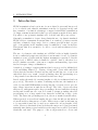
Automation of Testing of Polymer HVDC
Cables using Controlled Rapid Voltage
Surges.
Thomas Karlsen
Master of Science in Energy and Environment
Submission date: June 2007
Supervisor:
Erling Ildstad, ELKRAFT
Norwegian University of Science and Technology
Department of Electrical Power Engineering
Problem Description
Due to and commercialization of the energy markets and environmental considerations there is an
increasing interest in large-scale exchange of power between different countries and continents.
For the highest rated voltages in DC today, only oil-impregnated paper is utilized as cable
insulation. Extruded polymer solutions are currently beeing developed but many questions are
still unanswered. This is connected to among others, choice of testing methods for documentation
of high production quality and good long-term properties. The test procedure chosen must be
relevant regarding the service stress and sensitive for detection of production weaknesses.
In a NFR- and industrially supported project it is at NTNU/SINTEF beeing worked on developing a
simplified voltage surge technique for detecting insulation weaknesses in high voltage DC
insulation.
It has been shown that initiation of electrical trees in polymeric cable insulation can occur from
contaminations when beeing subjected to abrupt surges at a voltage significantly lower than the
breakdown voltage.
With basis in the developed experimental circuit, the student shall develop an automated system
that will replace the manual performing of subsequent rapid voltage surges and detecting cable
failures.
Assignment given: 15. January 2007
Supervisor: Erling Ildstad, ELKRAFT
Summary
This report aims to describe the work done in order to develop and create a
solution for automation of failure detection and performance of rapid voltage
surges. The automated system was developed with basis in the experimental
circuit developed at NTNU/SINTEF. The circuit relied on manually performing rapid voltage surges and detecting cable failure. Meaning that inequality
in the performance of each grounding may introduce unknow variables.
The realized automation system consisted of two parts. The first part was a
switch that was able to withstand the voltage applied and able to perform
the rapid voltage surges. The second part was a program that controlled the
switch and regularly monitored the condition of the cable object, indicating
failure when electrical treeing had caused breakdown in the cable insulation.
Two solutions for switches were examined. One switch utilized an arm moving between two electrodes for grounding the objects, using textile bakelite
as insulation and support frame for the electrodes. The other switch utilized
a sphere gap with air as insulation and an electric field strength close to the
breakdown strengt of the air. Groundings in the sphere gap switch were performed using a striker to greatly enhance the electric field and cause a spark
between the spheres, causing a transition from a highly insulating state to a
highly conductive state.
As the experimental circuit had a large current limiting resistance, the experimental circuit was sensitive to leakage currents as they set up a voltage
over the resistance, instead of the cable objects. Leakage currents in the
switches were examined and it was found that the arm switch had leakage
current unacceptable for use in the experiment. Similarly, leakage currents
in the sphere gap switch were examined and found to be acceptable for use
in the experiment.
The behaviour of cable objects that, due to electrical treeing had developed
insulation failure was examined and measurement parameters for detecting
cable failure were found. These parameters were implemented using LabView
as a platform for creating a a control program and interface to the instruments
connected to the switch.
Having fully created the automated system, the system was used in testing
cable objects and was found able to inflict and detect a cable failure due to
electrical treeing. However, compared to previous results, a lower number
of groundings was needed, which may indicate that the introduction of the
sphere gap switch has altered the circuit in a manner such that new results
i
will differ from former results.
ii
CONTENTS
CONTENTS
Contents
1 Introduction
1.1 Sample and electrode arrangement. . . . . . . . . . . . . . . .
1.2 Spark gaps . . . . . . . . . . . . . . . . . . . . . . . . . . . . .
2 Development and testing
2.1 General Program control . . . . . . . . . . . . . . . . .
2.1.1 Measuring current . . . . . . . . . . . . . . . .
2.1.2 Program requirements . . . . . . . . . . . . . .
2.1.3 Programdesign . . . . . . . . . . . . . . . . . .
2.1.4 Testing of the program . . . . . . . . . . . . . .
2.2 Arm switch . . . . . . . . . . . . . . . . . . . . . . . .
2.2.1 Design . . . . . . . . . . . . . . . . . . . . . . .
2.3 Sphere gap switch . . . . . . . . . . . . . . . . . . . . .
2.3.1 Design and simulation . . . . . . . . . . . . . .
2.3.2 Arrangement . . . . . . . . . . . . . . . . . . .
2.3.3 Control circuit . . . . . . . . . . . . . . . . . .
2.4 Testing . . . . . . . . . . . . . . . . . . . . . . . . . . .
2.4.1 Testing of withstand values . . . . . . . . . . .
2.4.2 Testing of leakage currents in the arm switch . .
2.4.3 Testing of leakage currents in the sphere switch
2.4.4 Testing of a cable object using the sphere switch
.
.
.
.
.
.
.
.
.
.
.
.
.
.
.
.
3 Results
3.1 Program . . . . . . . . . . . . . . . . . . . . . . . . . . .
3.2 Arm Switch . . . . . . . . . . . . . . . . . . . . . . . . .
3.3 Sphere switch . . . . . . . . . . . . . . . . . . . . . . . .
3.4 Closer examination of the undetermined leakaged current
.
.
.
.
.
.
.
.
.
.
.
.
.
.
.
.
.
.
.
.
.
.
.
.
.
.
.
.
.
.
.
.
.
.
.
.
.
.
.
.
1
2
3
.
.
.
.
.
.
.
.
.
.
.
.
.
.
.
.
4
4
4
6
8
14
15
15
19
21
22
22
26
26
27
27
28
.
.
.
.
30
30
31
33
37
4 Discussion
43
5 Conclusion
45
6 List of devices
46
A Monitor voltage and output current
48
B Maximum E-field at electrode surface
48
C Voltages measured with sphere switch
50
iii
LIST OF FIGURES
LIST OF FIGURES
List of Figures
1
2
3
4
5
6
7
8
9
10
11
12
13
14
15
16
17
18
19
20
21
22
23
24
25
26
27
28
29
Experimental circuit for use in testing. . . . . . . . . . . .
Currents measured in a cable with failure . . . . . . . . . .
ABC equvalent for measuring partial discharges . . . . . .
Shunt for measuring partial discharges . . . . . . . . . . .
Flowchart for the control program . . . . . . . . . . . . . .
Start loop of the program. . . . . . . . . . . . . . . . . . .
Labview implementation of equation 18. . . . . . . . . . .
Sequence of closing and opening the breakers. . . . . . . .
Front panel of the program . . . . . . . . . . . . . . . . . .
Electric field versus radii of electrodes. . . . . . . . . . . .
Electric field versus separation distance. . . . . . . . . . .
Contour of electric field for radius and separation distance.
Electric field between electrodes. . . . . . . . . . . . . . . .
Supportplate for switch electrodes. . . . . . . . . . . . . .
IEEE standard for vertical sphere gap . . . . . . . . . . . .
Electric potential when needle strikes . . . . . . . . . . . .
Electric field strength when needle strikes . . . . . . . . . .
Sphere gap arrangement . . . . . . . . . . . . . . . . . . .
Control circuit for needle . . . . . . . . . . . . . . . . . . .
Circuit for measuring current through sphere gap . . . . .
Monitor voltage versus output current . . . . . . . . . . .
Currents with and without armbreaker in circuit. . . . . .
Calculated voltage loss with armbreaker in circuit. . . . . .
Measured withstand values and table values . . . . . . . .
Breakdown channel in cable insulation . . . . . . . . . . .
Breakdown channel in cable insulation . . . . . . . . . . .
Measured current with no equipment connected. . . . . . .
Inner resistance of source . . . . . . . . . . . . . . . . . . .
Relation between monitor voltage and output current . . .
iv
.
.
.
.
.
.
.
.
.
.
.
.
.
.
.
.
.
.
.
.
.
.
.
.
.
.
.
.
.
.
.
.
.
.
.
.
.
.
.
.
.
.
.
.
.
.
.
.
.
.
.
.
.
.
.
.
.
.
2
5
7
7
9
10
10
11
12
16
17
17
18
19
21
22
23
24
24
28
30
32
33
35
36
38
39
40
41
LIST OF TABLES
LIST OF TABLES
List of Tables
1
2
3
4
5
6
7
8
9
10
11
12
13
14
15
16
17
18
19
20
21
22
23
Values of disruptive-discharge voltages valid for direct voltages
of either polarity. From [6]. . . . . . . . . . . . . . . . . . .
Measured current and deviation from calculated current. . .
Monitor voltages without any equipment, and with arm switch
in circuit. . . . . . . . . . . . . . . . . . . . . . . . . . . . .
Measured Gap distance and withstand voltage . . . . . . . .
Measured voltages from control circuit . . . . . . . . . . . .
Voltages measured with shortcircuited gap and the currents
they indicate . . . . . . . . . . . . . . . . . . . . . . . . . .
Deviation of measured currents from calculated current . . .
Calculated current and resistance in voltage divider . . . . .
Calculated currents through R1 . . . . . . . . . . . . . . . .
List of devices . . . . . . . . . . . . . . . . . . . . . . . . . .
Measured monitor voltage and calculated current. . . . . . .
distance = 0.075 m . . . . . . . . . . . . . . . . . . . . . . .
distance = 0.1 m . . . . . . . . . . . . . . . . . . . . . . . .
distance = 0.125 m . . . . . . . . . . . . . . . . . . . . . . .
distance = 0.15 m . . . . . . . . . . . . . . . . . . . . . . . .
distance = 0.175 m . . . . . . . . . . . . . . . . . . . . . . .
distance = 0.2 m . . . . . . . . . . . . . . . . . . . . . . . .
distance = 0.225 m . . . . . . . . . . . . . . . . . . . . . . .
distance = 0.25 m . . . . . . . . . . . . . . . . . . . . . . . .
Voltages measured with 3.69 cm gap distance . . . . . . . .
Voltages measured with 4.97 cm gap distance . . . . . . . .
Voltages measured with 7.10 cm gap distance . . . . . . . .
Voltages measured with shortcircuited gap. . . . . . . . . . .
v
. 20
. 31
. 32
. 34
. 35
.
.
.
.
.
.
.
.
.
.
.
.
.
.
.
.
.
.
37
37
41
42
46
48
48
48
49
49
49
49
49
50
50
51
51
52
1 INTRODUCTION
1
Introduction
HVDC transmission has been in use for more than 50 years and has proved
to be a reliable and valuable transmission media for electrical energy and
has a number of technical advantages compared with HVAC transmission
[2]. Improvements in material technology and extrusion methods have made
it possible to use polymeric insulation for both AC and DC power cables.
Currently, accumulation of space charge limits the use of polymeric insulated
HVDC cables to transmission systems that do not undergo polarity reversals
and have a limited voltage range. It is a common perception that one particle or irregularity in the insulation may be sufficient to cause breakdown.
This means that it is essential to be able to reveal such weaknesses before
installation.
The use of polymeric cable insulation for HVDC cables is highly desirable
from a commercial perspective and there is an incentive for use of polymeric
insulation even for cables with the highest transmission capacity, today the
voltage level of HVDC cables is limited to 600 kV. And so the there is a
need for further research to gain a more complete understanding of processes
involved in space charge accumulation.
A method of testing for such weaknesses has been proposed by Mildrid Selsjord and Erling Ildstad [7]. Testing of Rugowski objects with embedded
defects had shown that electrical treeing and breakdown can occcur at an
embedded defect as a result of rapid grounding after DC prestressing at a
voltage much lower that the short-term breakdown voltage.
Based on this, the method for testing lengths of cable for weaknesses has been
proposed [4]. The method consists of inserting needles into the insulation of
cable objects with XLPE insulation and poling the objects in order to provoke
space charge injections around the needle tip. The cable objects were then
subjected to subsequent rapid voltage groundings. It was found that electrical
treeing and breakdown can occur as a result of abrupt grounding after DC
pre-stressing at a voltage much lower than the breakdown voltage of the
cable. The faster the grounding was done, the more marked was this effect.
When repeated on several test lengths, the procedure should give information
about allowable working stress of a cable. If the test procedure would turn out
to be successful, it may also be used as a routine test on long lengths of DC
cables. However, this method involved that the surges are beeing performed
manually introducing several variables as the surges never will be performed
identically each time. The purpose of the work presented is to create and
1
1.1 Sample and electrode arrangement.
1 INTRODUCTION
test an automated method of executing the experiments using controlled
rapid voltages surges, by developing and creating a control program and a
high voltage switch.
1.1
Sample and electrode arrangement.
The proposed experimental method is described in [4]. Test objects are
made using using 1 m long sections of a 12 kV XLPE cable equipped with
terminations. In each test object, a sewing needle, with a tip radius of 50 µm,
and an overall diameter of 0.8 mm was at room temperature inserted through
the insulation screen and into the XLPE insulation. A mechanical tool was
specially designed to make reproducibly selected distances between the needle
tip and the conductor screen. In addition, a metallic mesh was clamped to
the insulation screen to fascilitate high frequency grounding of the screen and
needle.
Figure 1: Experimental circuit for use in testing.
Before grouding the cable objects, the applied voltage was increased to the
prestress level and held at this level for 24 hours. When closing the grounding
switch, the voltage was rapidly reduced to zero at a rate determined by the
capasitance of the test object and the impedance Z, of the grounding circuit.
The high voltage resistance of R = 2.005 GΩ made it possible to operate this
switch independent of the DC source and reduced the short-circuit currents
from the source.
2
1 INTRODUCTION
1.2
1.2 Spark gaps
Spark gaps
Simple spark gaps insulated by atmospheric air can be used to measure the
amplitude of a voltage above about 10 kV. As the fast transitions from an
either completely insulating or still highly insulating state of a gap to the
high conducting arc state is used to determine a voltage level, the disruptive
discharges does not offer a direct reading of the voltage across the gap. A
complete short-circuit is the result of a spark, and therefore the voltage source
must be capable to allow such a short-circuit, although the currents may and
sometimes must be limited by resistors in series with the gap.
Osmokrovic et al [10] used a three-electrode spark gap to create a method
of testing high-voltage circuit breakers with rated power values up to 25000
MVA under short-circuit conditions. As the maximum short-cirtuit power
obtainable from an actual grid was 6000 MVA, they increased the power by
building a synthetic circuit together with a direct test circuit. These were
synchronized using a three-electrode spark gap.
Two different types of three-electrode gas insulated spark gaps were used; a
spark gap with a third electrode beeing inside the main low-voltage electrode.
And a spark gap with a separate third electrode on floating potential. The
spark gap triggering was realized by applying a negative triggering pulse to
the triggering electrode, setting up a greater voltage difference than the DC
breakdown voltage and initiating a breakdown.
3
2 DEVELOPMENT AND TESTING
2
Development and testing
2.1
General Program control
Labview software was used to control and monitor the applying of rapid
voltage surges. The name is short for Laboratory Virtual Instrumentation
Engineering Workbench and is widely used for data acquisition, instrument
control, and industrial automation. It also features a platform for a visual
dataflow programming language similar to Matlab’s simulink.
The instrument chosen for controlling the test was a HP Agilent 34970A data
acquisition/switch unit. The intrument can communicate with a computer
using either a GPIB- or RS-232 interface [1]. In addition the instrument
is extensible with up to three plugin-modules. The two modules that were
chosen was a 20 channel armature multiplexer and a 4x8 two-wire matrix
switch. This enabled the control system to both measure voltages from up
to 20 inputs and perform any possible connection at 32 crosspoints in the
matrix switch1 .
2.1.1
Measuring current
As surges are applied, an eletrical tree will form from contaminations in
the cable insulation. Such contaminations will enhance the electric field,
causing partial discharges and a failure will occur. When this failure occurs,
a conductive breakdown channel will appear and a significantly larger current
will flow through the circuit.
In order to detect these failures, a spesific voltage given from the glassman
HV-source was used, the monitor voltage. The user manual [5], claims that
this monitor voltage is a 0 - 10 V signal in direct proportion to output current
from the source.
For determining the actual relation between monitor voltage and the output
current of the source, a circuit consisting of only two resistances was set up.
These resistances was the same as the current limiting resistances for testing
cable objects and had a value of 2 GΩ plus 5 MΩ. The applied voltage was
read from the display at the front panel of the source and the monitor voltage
was measured with the Agilent unit.
1
As the power needed to operate the circuit breakers will exceed the rated switching
values of the instrument, the matrix switch will route a 12 V signal to relays capable of
switching this power.
4
2 DEVELOPMENT AND TESTING
2.1 General Program control
For some of the applied voltages, the voltage over the resistance of 472.6 kΩ
was measured, and the belonging current was found. Also, the deviation
from the calculated current in table 11 was found. See table 2.
The total resistance would then be 2.005472600 GΩ, and the calculated current was found simply using ohms law:
calculated current [A] =
Applied voltage [V]
2.0054726 · 109 Ω
(1)
The applied voltage, the measured monitor voltage and the calculated current
can be seen in table 11 in appendix A.
A relation between the monitor voltage and the current in the circuit was
derived. As seen in figure 21, the approximation is fairly accurate. And this
relation was further used in the labview software as a method of determining
the output current from the source.
A cable with a known failure was inserted into the circuit and tested. The
resistance of the faulty cable was very low compared to the total resistance.
Following, the current through the cable was very similar to the current
measured when the circuit consisted only of the resistances. In figure 2 the
current through a faulty cable is plotted together with the current measured
when short-circuiting the cable object.
Figure 2: Currents measured in a cable with failure
5
2.1 General Program control
2 DEVELOPMENT AND TESTING
As seen in figure 2, a cable with a failure in the circuit, represented a connection from conductor to shield with no significant increase in the total
resistance, about 50 MΩ [11]. This meant that no significant decrease from
the short circuit current. When introducing a interval from the maximum
current, this was used as a parameter for detecting a cable failure.
2.1.2
Program requirements
Testing of a cable object consists of poling a cable object with needle implants
for 24 hours so that the slow polarisation mechanisms have decayed. When
this is done, the cable object is subjected to repeated negative rapid voltage
surges by bringing the conductor voltage to ground. This is done with a fixed
time interval. This performing of rapid voltage surges takes place until the
cable object grow electrical trees and an electrical breakdown occurs.
It is the intention that when the cable breaks down, the failure shall be
detected by the program and the number of groundings displayed. Each
measurement as well as the number of grounding were to be displayed on a
graph and later stored in a datafile.
As the current that flows through the point of failure will vary, it is desired
that the failure indicating interval is adjustable from the user panel of the
program.
Additionally it is desired to measure any partial discharges that may occur
in the initial growth of the electrical tree. This measurement would done by
using the abc-equivalent of an initial electrical tree, see figure 3.
A rough calculation of the needed sensitivity can be done when using the
eqution for stored energy in a capacitor Q = C · U and assuming the capacitance cable of the cable as 200 pF and the dissipated charge in a partial
discharge as 1 pC. The measurment equipment will be performed in another
project but as the same control software will be used, the implementation
was done here/now.
U=
Q
1 · 10−12 C
1
=
=
V = 5 mV
−12
C
200 · 10 F
200
(2)
As the equipment for measuring these partial discharges needs to be very
sensitive, the shunt needs to be protected during the relatively violent voltage
surge. This was done by inserting a breaker B1, that protects the shunt by
connecting it to ground it as shown in figure 4, and creating a alternate path
6
2 DEVELOPMENT AND TESTING
2.1 General Program control
Figure 3: ABC equvalent for measuring partial discharges
for the current. The required action of the program is to close this breaker
before the surge and then open it after the surge.
Figure 4: Shunt for measuring partial discharges
All these requirements for the program and control circuit was summarized
into the follows:
• Perform the desired number of voltage surges until failure.
• The voltage surges shall be performed with a fixed intervall.
• Regularly check for failure between the surges.
• Protect the equipment measuring partial discharges.
• Display the measurements.
• Save the measured data to a file.
7
2.1 General Program control
2.1.3
2 DEVELOPMENT AND TESTING
Programdesign
In order to better structure the requirements and behaviour of the control
program, a flowchart was needed in order to perform the design. A flowchart
is a schematic representation of the process, and helps creating the program
code. This is especially useful when programming in labview, which is a
visual programming language. When applying the requirements listed earlier,
a flowchart was drawn as in figure 5.
The flowchart summed up the main tasks to be performed by the program.
However, due to the nature of the programming language in labview, the
program itself needed to be more complex.
From the flowchart, the program was divided into three sections. The first
section took care of the ”start test” part in the flowchart. In this section, all
the necessary input parameters are collected before continuing. The realization of this was to use a while-loop that runs continuously until a start-button
is pressed. This loop collects the parameters and initiates the main part of
the program when the button ”Start test” is pressed, see figure 6.
It would be convinient only to enter the applied voltage as a parameter for
determining the maximum current. But as the current limiting resistances
can be replaced, this is entered in addition to the applied voltage. Further the
relation in equation 18 was implemented for finding the belonging monitor
voltage, see figure 7.
When the start-button is pressed, the parameters are collected and a VISA
2
connection to the instrument is created. When this is done, the program
exits the inital loop and the second part of the program is started.
The second and main section of the program took care of the two loops that
can be seen in the flowchart, figure 5. In this section, groundings and failurechecks are performed. Groundings are performed by routing a 12 V signal to
a relay, using the 4x8 matrix switch.
The realization of the second section, and main part of the program, was
done using two nested loops. The outermost is a for-loop that is governed
by the execution of surges and runs for the number of times set in ”number
of surges” at the start of the program. The innermost is a while-loop that is
governed by the measurements performed between the surges.
When in the while-loop, the program will measure the monitorvoltage using
the 20-channel multiplexer and use this to check for cable failure. This will
2
Virtual Instrument Software Architecture
8
2 DEVELOPMENT AND TESTING
2.1 General Program control
Figure 5: Flowchart for the control program
9
2.1 General Program control
2 DEVELOPMENT AND TESTING
Figure 6: Start loop of the program.
Figure 7: Labview implementation of equation 18.
10
2 DEVELOPMENT AND TESTING
2.1 General Program control
be done with a fixed interval until it is time to perform the next grounding.
The time between each measurement is set from ”measure interval” at the
front panel of the program. The currents indicated by the measured monitor
voltage is displayed as a graph in the rigth section of the frontpanel. If a
failure is detected, the program will close the breaker protecting the pd-shunt,
open the latch, show a message dialog and stop.
When the surge interval has elapsed and no failure has been detected, the
program exits the inner while loop and performs a grounding. The performance of a grounding is a realized with a sequence of closing and opening
the two relays, B1 and B2, see flowchart 5. At first, the relay that protects
the pd-shunt, B1, is closed. Then the program waits a time ”shunt w-time”
before closing the relay B2, that performes the actual grounding. When the
program then has waited the ”coil discharge time”, it opens the relay B2, and
again waits the time ”shunt w-time” before opening the relay B1. See figure
8 for the realization of the sequence in labview.
Figure 8: Sequence of closing and opening the breakers.
When grounding has been performed, the for loop either continues or exits.
This is dependent on whether the desired number of groundings has been
reached or not. If not, the for-loop continues. And if the desired number
of groundings has been performed, the program closes the breaker that is
protecting the pd-shunt, opens the latch and stops.
When the Labview code of the program was fully created, a front panel was
designed. The front panel is the graphical user interface used when running
the program and synthesises the behaviour of a real instrument. For this
reason it is also called a virtual instrument, [8].
Mainly, the front panel consists of datafields for entering the parameters
that are required in the inital while-loop, see figure 6. It also includes an
11
2.1 General Program control
2 DEVELOPMENT AND TESTING
area that shows the progress of the test and an area that displays the latest
measurements of output current. See figure 9 for the design of the front
panel.
Figure 9: Front panel of the program
The program controls four channels on the Agilent instrument. One for
measuring the monitor voltage, the second for triggering the switch and the
fourth for protecting the equipment for measuring partial discharges. The
third is optional and can be used for latching of the HV-source when the
program has detected a failure in order to stop the current flowing through
the cable insulation.
All the datafields in figure 9 is explained as follows:
VISA resource name This is the field for specifying the GPIB-adress for
the instrument. This value must be the same as the value set at the
instrument as there can be several instruments connected to the same
cable. Default GPIB channel is set to 9.
Reset This is an option whether to reset the instrument when connecting
to it. Default is ”Don’t reset”. Note that this may cause problems if
the latch is connected.
Serial Port Configuration This is the configuration when using a RS232
connection instead of a GPIB connection. Default values are set.
Last error out This is a message box that displays the last error message
generated. By default, no errors have occured and the box is empty.
12
2 DEVELOPMENT AND TESTING
2.1 General Program control
In case a error has occured, the program should be restarted in order
to clear errors and measurement data.
Number of surges This is the desired number of surges that is to be performed. Default is set to a high number, 150000 surges.
Measure interval This is the interval between each check for failure. Default is set to 2000 ms
Surge interval This is the interval between each voltage surge. Default is
set to 60 s
Surge wait period When the cable has been subjected to a grounding, a
higher current will flow in order for the cable to recharge. Measuring
the current in this period may falsely indicate a failure. The wait period
is the time the program waits until beginning to chech for failure again.
Default is set to 4 s
Coil discharge time This is the on-time of the switch, depending on its
type type. Default is set to 0.5 s
Shunt w-time This is the time before the surge, that the shunt for measuring partial discharges is protected. This equals the ∆t in figure 5.
Default is set to 0.1 s
Scanlist - measure The scanlist, indicating where the monitorvoltage is
connected. Default is set to channel 205.
Scanlist switch This is the scanlist, indicating where the 12 V is routed to
the switch. Default is set to channel 138.
Scanlist shutdown This is the scanlist, indicating where the latch of the
HV-source should be connected. This is optional and default is set to
channel 148.
Scanlist shuntprotection This is the scanlist, indicating where the breaker
for protecting the pd-equipment is connected. Default is set to channel
137.
Applied voltage [V ]This is the applied voltage to the circuit and is used
for determining the maximum current. Default value is set to 60 kV
Resistance [Ohm ]This is the total value of the current-limiting resistances
and is used for determining the maximum current. Default value is set
to 2.005 GΩ
13
2.1 General Program control
2 DEVELOPMENT AND TESTING
Fault interval This is the interval used for detecting a failure. When a
monitor voltage larger than the product of fault interval and the predicted monitor voltage is measured, the program states that a failure
has occured. Default is set to 0.9.
Resolution This is the instrument resolution for voltage measurements. Default is set to the default setting of the instrument.
Range This is the instrument range for voltage measurements. Default is
set to Auto.
N - averaging To avoid beeing mislead by misreadings, one can average
over the last measurements in order to better determine a failure. When
averaging is used, the average value has to be larger than the product
of the fault interval and the predicted monitor voltage. By default, the
five last measurements are averaged.
While-loop iteration This is the counter for the while loop and displays
the current iteration.
For-loop iteration This is the counter for the for-loop and displays the
current iteration.
Overall progress This is a progress bar that displays the progress of the
test.
Stop test This is a button that stops the test. It is recommended to use
this in order to perform the exiting routines.
Test started This is an indicator that shows whether the test has started.
Failure detected This is an indicator that shows whether a failure has been
detected.
Test stopped This is an indicator that show whether the test has stopped.
Plot area This is a graph that displays the measurements of the monitor
voltage. The same values are saved to the xml-file.
2.1.4
Testing of the program
During the design process, the program was continuously tested by using a
imitated value instead of the real measurement of the monitor voltage. When
the program itself worked according to the specitications, the communication
with the instrument was tested.
14
2 DEVELOPMENT AND TESTING
2.2 Arm switch
In order to test the voltage measured from the Agilent instrument, a variable
low voltage source that could deliver up to 30 V was used to imitate the
monitor voltage. The part of the program that checked for failure was finally
tested against the glassman voltage source and a cable with a failure.
2.2
Arm switch
A previously used circuit breaker was found to have leakage currents when
applying higher voltages. These leakage currents set up a significant voltage
over the current limiting resistances. As the applied voltage over the switch
increased, the leakage current and hence the voltage over the resistances
increased. The voltage over the cable object never reached more than about
40 kV, see [11]
In order to remove this effect of voltage loss, the arm switch was to be
modified into a switch with lesser leakage currents.
2.2.1
Design
The initial design was performed with FEMLAB/MATLAB software.
The original switch consisted of a fibreglass plate that held the two electrodes
in place. An arm was moved between the electrodes using an actuating coil.
The electrodes themselves had a radius of about 0.5 cm. This caused a
divergent electric field and a region with high electric stress at the surface of
the electrodes.
In order to achieve lesser leakage currents, three main goals were defined for
the new design.
• larger radii of the electrodes and edges of the conductive materials.
• larger separation of electrodes in air.
• larger creep distance in the plate between electrodes.
To obtain an initial, but absolutely not final value of the distance between
the electrodes for use in the simulation software, the breakdown strength of
air was set to 3.2 · 106 V/m. This gives the distance:
d=
U
200 · 103 V
= 0.0625m
=
Emax
3.2 · 106 V /m
15
(3)
2.2 Arm switch
2 DEVELOPMENT AND TESTING
A model of two round electrodes were modeled in Femlab. The electrodes
were aligned vertically and for fixed separation distances S, between 0.075 m
to 0.3 m, the radius was varied from 0.01 m to 0.05 m and the maximum
electric field was noted down. The electric field strength was typically highest
at the surface of the high voltage electrode. The values are shown in tables
12 - 19 in appendix B.
The results from the simulation were plotted and visualized in matlab. In
figure 10 one sees that for all radii, the maximum electric field decreases less
as the separation disctance between the electrodes increases.
Figure 10: Electric field versus radii of electrodes.
Similar behaviour is seen for the radius of the electrodes, see figure 11. For
all separation distances, the maximum electric field decreases less as the radii
of the electrodes increases. A good choice of radius and separation distance
would be in the area where the maximum electric field is satisfactory low and
the dimensions are kept sensibly low.
For better visualisation of the resulting electric field for different values of
radius and distance, a contour-plot was plotted for values between 16 kV/cm
and 36 kV/cm, see figure 12.
An electrode radius of 0.03 m, and a electrode distance of 0.2 m was chosen
based on the availability in the workshop. From the simulation, this gives
a maximum electric field of 22 kV/cm at the surface of the HV side of the
switch. This configuration is also plotted in figure 12. The actual electric
16
2 DEVELOPMENT AND TESTING
2.2 Arm switch
Figure 11: Electric field versus separation distance.
Figure 12: Contour of electric field for radius and separation distance.
17
2.2 Arm switch
2 DEVELOPMENT AND TESTING
field strength along the axis between the centers of the two electrodes can
be seen in figure 13. The maximum field strength appears at the surface of
the top electrode and is significantly less at the lower electrode. This gives
greater tolerances for edges at the arm when the switch is open.
Figure 13: Electric field between electrodes.
A supportplate for the electrodes was designed as in figure 14. The available
material for the plate was textile bakelite. This material is often used as
insulation for high voltage equipment, as it can endure temperatures up to
120 ◦ C.
The only obtainable material spesification from the supplier was that the
electrical breakdown strength is 5 kV for 3 mm. The conductivity of the
material was unknown.
In the model, see figure 14, the shortest distance between the high-voltage
and the ground electrode is about 16 cm. The withstand voltage the plate
should then be
Ubakelite =
5kV
· 160mm = 266kV
3mm
18
(4)
2 DEVELOPMENT AND TESTING
2.3 Sphere gap switch
Figure 14: Supportplate for switch electrodes.
2.3
Sphere gap switch
As the arm switch had several divergent fields that were hard to control, a solution with a more homogenous field distribution was needed. Kuffel et al [3]
discusses several arrangements for reliably measuring high voltages. Mainly
the rod/rod gap and the sphere gap are recommended as their reliabilities
are best confirmed.
Rod gaps have earlier been used for for the measurement of impulse voltages, but because of the large scatter of the disruptive discharge voltage and
the uncertainties of the strong influence of the humidity, they are no longer
allowed to be used as standard measuring devices.
A sphere gap was therefore preferred, as limitation in the gap distance provides a homogenous field distribution between the spheres so that no predischarge or corona appears before breakdown. The measuring capability of the
sphere gap was not to be used, but the ability to apply maximum voltage
before breakdown.
Two methods of modifying a sphere gap into a three-electrode spark gap has
been described by Osmokrovic et al [9], but required a relatively complex
arrangement. A a simpler mechanism of extending the trigger electrode into
the sphere gap, would provide similar effect, as the electric field is rapidly
increased above withstand level.
A complete short-circuit is the result of a spark. The experimental circuit
19
2.3 Sphere gap switch
2 DEVELOPMENT AND TESTING
has a current-limiting resitance and the voltage source is therefore capable to
allow such spark. This would be a good method for performing rapid voltage
surges to the cable objects.
The IEEE standard for High-Voltage Testing, [6], defines the standard sphere
gap as a peak-voltage measuring device constructed and arranged in accordance with the standards spesifications. It consists of two metal spheres of
the same diameter, D, with their shanks, operating gear, insulating supports,
supporting frame, and leads for connections to the point at which the voltage
is to be measured.
Standard values of sphere diameter, D, vary from 62.5 mm to 2000 mm. The
spacing between the spheres is designated as S, and varies from 5 mm to
2000 mm. The voltages to be measured with these configurations vary from
69.5 kV to 2490 kV, see table 8 in[6]
Spheres with a diameter of 250 mm were available at the Elkraft engineering
workshop. The Glassman HV source provides a dc voltage of up to 200 kV.
For the given sphere diameter within this voltage range, the gap distances
varies from 25 mm to 80 mm, see table 1.
Table 1: Values of disruptive-discharge voltages valid for direct voltages of
either polarity. From [6].
Sphere gap spacing (mm) Voltage (kV peak)]
25
72.5
30
86.0
35
40
112
45
50
137
55
60
161
62.5
70
184
80
206
The point on the two spheres that are closest to each other are called sparking points and is where the breakdown occurs. In practice, the disruptive
discharge may occur between other neighbouring points. But in the realizede
switch, a spark will be initiated by rapidly increasing the electric field by
moving a striker with a relatively small radius into the electric field between
the spheres.
20
2 DEVELOPMENT AND TESTING
2.3 Sphere gap switch
An arrangement, which is typical of sphere gaps with a vertical axis, is shown
in figure 15. One sphere shall preferably be connected directly to ground
but it may be connected through a resistance for special purposes such as
measuring the current when sparks occur. In the interests of personnel and
equipment safety, such resistances should be of very low values.
Figure 15: IEEE standard for vertical sphere gap
2.3.1
Design and simulation
The sphere gap arrangement was drawn and simulated with Comsol Femlab
software. The model was drawn with the striker pin extended from the
lower sphere into the sphere gap. The model was solved and the electric field
distribution and the electric potential distribution was found for a case where
86 kV were subjected to a sphere gap distance of 30 mm according to table
1, see figure 16.
It was found that the electric field strength was greatly enhanced at the tip
21
2.3 Sphere gap switch
2 DEVELOPMENT AND TESTING
Figure 16: Electric potential when needle strikes
of the striker. A maximum value of the field was found to be as much as
4.6 kV/cm, see figure 17. Finding this, further work with the realization of
the switch was performed.
2.3.2
Arrangement
An arrangement consisting of a sphere and a half sphere was set up. The
top sphere was connected to the HV side and subjected to the same voltage
as the cable objects that were beeing tested. The bottom half sphere was
connected directly to ground. The bottom sphere featured the striker that
would be used to rapidly create a divergent eletric field, see figure 18. A coil
surrounding the striker and would be used to raise the needle into the gap
between the spheres.
When the needle is extended into the gap, the electric field around the tip
is enhanced above the withstand voltage of the surrounding air. This causes
the air to break down and a discharge occurs in the gap between the two
spheres.
2.3.3
Control circuit
The lower sphere contained a setup of a striker surrounded by a coil. When
a current is led through the coil, the needle is forced up by the magnetic
22
2 DEVELOPMENT AND TESTING
2.3 Sphere gap switch
Figure 17: Electric field strength when needle strikes
field. The power needed to actuate the striker was not available from the
instrument and therefore a designated electric circuit was created for this
purpose, see figure 19.
The Agilent instrument was to control the circuit, routing a 12 V signal to a
relay. In order to provide a sufficient amount of energy for the coil to extend
the needle, capasitors were to be charged up and disharged over the coil. To
charge the capasitors, ac voltage was taken from the grid and transformed
down with a 2:1 transformer. Using a fullbridge rectifier the capasitors was
charged from both half-waves of the voltage from the transformer.
The energy used when extending the needle would come from the charged
capasitors. But in the case of a relay fault, a larger current than intended will
flow from the transformer to the coil. Therefore a current limiting resistance
R, was inserted in order to prevent the current from exceeding the maximum
rated current of the transformer. In addition, fuses were inserted as a general
mean of protection.
In order to find a suitable value for the resistance, two relations were to be
considered. Firstly, the time constant of the circuit had to be small enough
so the capacitors would be fully charged before a grounding were performed.
23
2.3 Sphere gap switch
2 DEVELOPMENT AND TESTING
Figure 18: Sphere gap arrangement
Figure 19: Control circuit for needle
24
2 DEVELOPMENT AND TESTING
2.3 Sphere gap switch
Secondly, the resistance had to be large enough so that the transformer did
not deliver more than rated current if the relay was to be closed for a longer
period than intended.
The capasitors had to be fully charged within shorter time than the grounding interval of the cable objects, usually 60 s. When the relay is open, the
capacitors C, are in series only with the resistance R, and the belonging time
constant is τ = R · C. Given that the capacitanse is 136 µF, the largest
resistance with respect to the first relation is:
R=
τ
60s
=
= 441176.5Ω
C
136 · 10−6 F arad
(5)
The datasheet for the transformer states that the rated current for the secondary side of the transformer is 250 mA. The rectifier has a rated current
of 3 A so the transformer sets the current limit. The rectified voltage over
the capasitors was measured to be 177.1 V and the smallest resistance with
respect to the second relation was:
R=
177.1V
= 708.4Ω
0.25A
(6)
The resistance therefore had to be between 710 Ω and 440 kΩ. A 5 W resistance of 56 kΩ was selected.
In order to protect the circuit itself and connected equipment from incoming
overvoltages, five surge arresters were inserted at two places, see figure 19. For
protection of the Agilent unit, the two wires connected to the 12 V relay were
protected with S1 and S2, having the smallest available protection level of
75 V. The multiplexer can withstand voltages up to 300V and it is therefore
assumed able to handle transients up to 75 V.
The output of the circuit was also protected with surge arresters. The protection level of S3, S4 and S5 was set to 225 V, enough to allow the voltage
over the charged capacitors to operate the coil surrounding the striker, but
also protecting the circuit from incoming overvoltages.
25
2.4 Testing
2.4
2.4.1
2 DEVELOPMENT AND TESTING
Testing
Testing of withstand values
A simple test of the withstand values for the sphere gap was performed.
According to table 1, the gap distance varies between 2.5 cm and 8.0 cm for
the voltages available from the HV source. The sphere gap were adjusted
to three different distances within this range, 3.77 cm, 5.02 cm and 7.35 cm.
The voltage was then raised until a spark occured in the gap and noted down,
see table 4.
Using the values in [6], the breakdown values corresponding to the distances
was found using linear interpolation; for a point (x, y) at a straight line
between to points (x0 , y0 ) and (x1 , y1 ), the linear relation yields:
x − x0
y − y0
=
=α
y1 − y0
x1 − x0
(7)
For each gap distance, the α from the table was calculated:
3.77 − 3.5
= 0.54
4.0 − 3.5
5.02 − 5.0
= 0.04
α2 =
5.5 − 5.0
7.35 − 7.0
α3 =
= 0.70
7.5 − 7.0
α1 =
(8)
(9)
(10)
Equation 7 was rewritten into:
y = y0 + α(y1 − y0 )
(11)
Using these values and equation 11, the corresponding breakdown values was
found and is shown in equations 12 - 14.
T1 = 99 + 0.54(112 − 99) = 106.02
T2 = 137 + 0.04(149 − 137) = 137.48
T3 = 184 + 0.70(195 − 184) = 191.7
26
(12)
(13)
(14)
2 DEVELOPMENT AND TESTING
2.4 Testing
The percentual deviation of the measured values from the interpolated values
was found using equation 15, see alignment 21 - 23.
deviation =
Umeasured − Ttable
· 100
Ttable
(15)
.
2.4.2
Testing of leakage currents in the arm switch
The only known electric property of the textile bakelite used for the arm
switch plate, was the breakdown voltage. This was assumed to be a value
that is valid for ac voltages only. The dc conductivity was unknown and a
testing of any eventual leakage current between the electrodes was performed.
The monitor voltage from the voltage source indicated a current flowing even
when no equipment was connected to the high voltage side of the source. As
this was a current not accounted by any apparent path, it was believed to be
discharges into air. Therefore the currents where measured with and without
the breaker in circuit, and the difference between them assigned to leakage
in the breaker.
In order to verify the measurements when inserting the breaker, a resistance
of 472.6 kΩ was connected betweeen the low voltage electrode and the ground.
In order to protect the multimeter in case of discharges, the resistance was
protected with a surge arrester with a protection level of 75 V. Voltage over
this resistance was measured and the actual current was found using Ohms
law.
Voltages from 0 kV to 120 kV was applied and the belonging monitor voltage
was measured from the glassman source, see section 3.2.
2.4.3
Testing of leakage currents in the sphere switch
A set of measurements was performed in order to determine the leakage
currents through the sphere gap. The multimeter was connected to the lower
side of the sphere and protected with a gas arrester in case of discharge. The
protection level of the arrester was 75 V. The resistance was inserted into
the circuit as R2 in figure 20.
The currents was measured for three gap distances, 3.69 cm, 4.97 cm and
7.10 cm. Three voltages was measured; the voltage applied, the monitor
27
2.4 Testing
2 DEVELOPMENT AND TESTING
Figure 20: Circuit for measuring current through sphere gap
voltage from the source and the voltage over the resistance R2. As the
voltages measured over R2 were too small to be correctly measured by the
multimeter, the gap was short-circuited in order to achieve larger currents.
These were compared to the monitor voltage in order to verify the currents
. See tables 20 - 23 appendix C.
2.4.4
Testing of a cable object using the sphere switch
A cable object was tested using the sphere switch and the program developed
in LabView. The applied voltage was 60 kV, the sphere gap distance was set
to the lowest in table 1, and the maximum current at failure would then be:
Imax =
60 · 103 V
= 29.93µA
2.005 · 109 Ω
(16)
The belonging monitor voltage, the failure parameter, was found applying
the relation in equation 18:
Um = 13787 · 29.92µA + 0.01 = 0.4226V
(17)
This value was used as the monitor voltage indicating failure and entered
into the program. The rest of the default values was not altered.
28
2 DEVELOPMENT AND TESTING
2.4 Testing
A needle was inserted into the insulation of the cable object. The cable object
was then connected to the sphere switch in series with a resistance of 93.3 Ω.
This resistance was placed in the circuit in order to control the front time of
the grounding pulse.
After poling, the cable object was subjected to rapid voltage surges using the
sphere switch and the program created in labview.
29
3 RESULTS
3
3.1
Results
Program
The measured monitor voltage was plottet against the calculated current
in the circuit using Matlab, see figure 21. The regression tool in Matlab
yielded a linear relation between monitor voltage and output current found
in equation 18.
Figure 21: Monitor voltage versus output current
Um (I) = 13787 · I + 0.01[V]
(18)
For some of the applied voltages, the voltage over the resistance of 472.6 kΩ
was measured, and the belonging current was found. Also, the deviation
from the calculated current in table 11 was found, see table 2.
The deviation was found to be small, no more than 1.8 %. When implementing the measurement of monitor voltage and using a interval from maximum
30
3 RESULTS
3.2 Arm Switch
Table 2: Measured current and deviation from calculated current.
U [kV] Measured Voltage [V] Measured current [microA] Deviation
0
0.001
0.002
20
4.79
10.14
1.6 %
40
9.38
19.85
0.5 %
60
14.15
29.94
0.1 %
70
16.20
34.28
1.8 %
current in circuit, the program correctly detected a failure.
3.2
Arm Switch
In order to improve a previously used armswitch, a new design was created
and tested. Using Comsol/Femlab software, the electric field distribution
around two electrodes was plottet for a set of different sizes and distances of
the actual electrodes. In all cases the highest values appeared at the surface
of the top HV electrode facing the lower electrode.
A configuration of electrode radius equal to 0.03 cm and an electrode separation equal to 0.2 m was chosen, based on the availiability in the workshop
and the mapping of results from the simulations.
Apart from the breakdown strength, electrical properties for the material
used making the armbreaker plate were unknown. This caused great uncertainty regarding the voltage loss over the current limiting resistances, and
actual voltage applied to the cable objects.
Two sets of measurements were performed. The first with nothing connected
to the source and the second with the arm switch connected to the circuit.
The monitor voltage was measured in both cases, and when connected, also
the voltage over R = 472.6 kΩ, see table 3.
Considering the effect of the switch, there was a significant change in current
when applying more than 40 kV. Also when increasing the applied voltage,
the difference between currents increased. The currents were calculated using
equation 18 plotted using matlab, see figure 22.
In order to determine the voltageloss over the current-limiting resistance, the
difference between the currents in figure 22 was multiplied with the resistance of 2.005 GΩ. In addition, the voltage over R2 was measured by the
multimeter was used to find a comparable voltageloss, applying the relation:
31
3.2 Arm Switch
3 RESULTS
Table 3: Monitor voltages without any equipment, and with arm switch in
circuit.
Applied voltage Um (nothing connected) [V] Um (breaker connected) [V]
0
0.015
0.014
20
0.044
0.045
40
0.083
0.091
60
0.113
0.183
80
0.186
0.263
100
0.231
0.352
120
0.273
0.454
Figure 22: Currents with and without armbreaker in circuit.
32
Ur [V]
0
0.044
0.447
1.28
2.29
3.78
5.9
3 RESULTS
3.3 Sphere switch
Uloss = Icircuit · 2.005 · 109 Ω =
Ur
· 2.005 · 109 Ω
3
472.6 · 10 Ω
(19)
The voltage loss indicated by these two measurements was plottet with matlab, see figure 23.
Figure 23: Calculated voltage loss with armbreaker in circuit.
Using the arm switch in the circuit, the voltage loss was quite significant.
When applying a voltage of 50 kV the voltage loss was about 3 kV and when
applying 100 kV, the voltage loss was about 16 kV. A relation between the
applied voltage and the voltage loss was found, see equation 20.
Uloss (U0 [V]) = 2.04 · 10−6 · U02 − 0.04 · U0 + 133[V]
3.3
(20)
Sphere switch
Due to the uncertainty of the arm switch, a more reliable alternative was
needed. With basis in the IEEE publication ”Standard Techniques for High33
3.3 Sphere switch
3 RESULTS
Voltage Testing” a switch based on a sphere gap was created. The sphere
gap used air as insulation material, and a more homogenous field distribution
was provided than for the arm switch.
As a mechanism of applying the rapid voltage surges, a striker with a small
tip radius was extended from the lower sphere into the gap. The electric field
at the tip of the striker became so enhanced that the air broke down and an
arc formed between the upper sphere and the striker tip.
As the impedance in figure 1 originally was connected between the lower
sphere and ground, a voltage was set up over this as the grounding were
performed. It was found that this voltage travelled back through the wires
and discarged in the surge arresters, rendering the effect of the impedance
useless. This was solved with placing the impedance between the HV-part of
the switch and the cable object.
Additionally, on one occasion unexpected disharges occured at a sphere gap
with sufficient distance and without the striker extended. This was later
found to be caused by a strand of hair that was situated on top of the lower
sphere.
The IEEE publication supplied known withstand values for different setups
of sphere diameter and sphere separation. And the measured withstand
voltages of the sphere gap switch deviated no more than 3.58 % from the
table values in [6], see table 4.
Table 4: Measured Gap distance and withstand voltage
Arch gap [cm] Withstand voltage [kV]
3.77
110
5.02
140
7.35
190
110 − 106.02
· 100 = 3.58%
106.02
140 − 137.48
D2 =
· 100 = 1.83%
137.48
190 − 191.70
D3 =
· 100 = −0.89%
191.70
D1 =
(21)
(22)
(23)
In order to visualize, the measured withstand values was plotted and compared to the table values using matlab, see 24.
34
3 RESULTS
3.3 Sphere switch
Figure 24: Measured withstand values and table values
The striker mounted in the lower sphere needed a more elaborate control
system than provided by the relay and labview program. Hence a control
circuit was created and tested.
Having designed the control circuit, the circuit was created and tested for
faults with a simple voltmeter. When connected to the grid, the circuit
worked properly and the needle stroke as intended. The input voltage was
measured to 224.6 V. On the secondary side, the voltage was measured to
129.9 V. This gives the transformer a more accurate ratio of 1.73:1. The
rectified dc voltage was also measured.
Table 5: Measured voltages from control circuit
Point of measurement Measured voltage [V]
input voltage
224.6 VAC
transformed voltage
129.9 VAC
rectified voltage
177.1 VDC
The leakage currents of the sphere gap switch was measured using both the
monitor voltage and the voltage that appeared over a resistance of 472.6 kΩ,
see tables 20 - 22. The actual current measured through the sphere gap was
found to be insignificant compared to the output current indicated by the
glassman source. This is illustrated in figure 25 where the graphs are at the
bottom are the currents measured by the multimeter.
35
3.3 Sphere switch
3 RESULTS
Figure 25: Breakdown channel in cable insulation
In table 21 and table 22 the voltage over the resistance R2 variated so much
that the value was unable to be read. This occured when about 110 kV
and more was applied. There was also audible corona at these voltages.
The largest voltage measured over the resistance was 0.003 V when applying
100 kV over a sphere gap of 4.97 cm. This indicated that a current of
I=
0.003V
= 6.35 · 10−9 A
3
472.6 · 10 Ω
(24)
was flowing through the gap.
Assuming that the same current flows through the current-limiting resistances, the voltage loss would be:
Uloss = 6.35 · 10−9 A · 2.005 · 109 Ω = 12.73V
(25)
This value was considerably less than the voltage loss of 16 kV that occured
when applying 100 kV to the arm switch.
The values read from the multimeter were very small and in order to get
comparative data the sphere gap was short-circuited and measurements performed. Using the short-circuit measurements in table 23, the indicated
currents were compared to the calculated currents, see table 6.
In table 7 the deviation of the measured currents from the calculated current
is shown, after applying equation 26.
deviation [%] = |
Icalculated − Imeasured
| · 100
Icalculated
36
(26)
3 RESULTS3.4 Closer examination of the undetermined leakaged current
Table 6: Voltages measured with shortcircuited gap and the currents they
indicate
calculated current[µA] current through R2 [µA] current indicated by source [µA]
0
0.00317
0.29
9.97
10.14
7.35
19.95
19.85
19.79
29.92
29.94
30.38
34.90
34.27
34.87
Table 7: Deviation of measured currents from calculated current
Calculated current [µA] Deviation R2 Deviation Glassman source
0
9.97
1.71 %
24.37 %
19.95
0.50 %
0.80 %
29.92
0.03 %
1.50 %
34.90
1.78 %
0.09 %
As the sphere gap was found to have insignificant leakage currents, testing
of a cable object was performed. The program detected a failure after 70
groundings. After slicing the cable object with a microtome, it was found
that the distance from the needle tip to the inner semiconductor was about
3 mm, see figure 26
For this length, fronttime and voltage, the expected number of groundings
was in the area of 60-100 groundings.
3.4
Closer examination of the undetermined leakaged
current
Undeterminable leakage currents was indicated by the voltage source. As
no equipment was connected to the source, the monitor voltage indicated
an output of as much as 15.88 µA when applying 100 kV, 25.45 µA when
applying 160 kV and as much as 31.54 µA when applying the maximum
voltage of 200 kV, see figure 27. If this current was flowing through the
circuit, is would case great voltage losses and a reduced voltage applied to
the cable objects.
Even though a current was indicated, this was not the same as measured in
the actual circuit. The sphere gap was found to have insignificant leakage
37
3.4 Closer examination of the undetermined leakaged current3 RESULTS
Figure 26: Breakdown channel in cable insulation
38
3 RESULTS3.4 Closer examination of the undetermined leakaged current
Figure 27: Measured current with no equipment connected.
39
3.4 Closer examination of the undetermined leakaged current3 RESULTS
currents when subjected to voltage. The armswitch had significant leakage
currents that corresponded only to the increase in monitor voltage, but not
the total current indicated by the monitor voltage.
After a more thorough inspection of the circuit schematics of the voltage
source, a voltage-divider was found to be present inside the source, as in
figure 28. The purpose of this voltage divider was to derive a feedback signal
for monitoring the real output voltage.
Figure 28: Inner resistance of source
The actual value of the resistance in the divider was not described in the
manual. However, the manual stated that a signal varying from 0 V to 10 V
is in direct proportion to the output current.
Assuming that a monitor voltage of 0 V indicates no current, and a monitor voltage of 10 V indicates the rated current of 1 mA as in figure 29, the
assumed relation between monitor voltage and output current was described
as in equation 27.
I=
Um
· 0.001
10
(27)
In order to determine the value of R1 figure 28, the values in table 23 was
used, except the measurement for zero applied voltage. These measurements
were done with the known R2 equal to 2.0054726 GΩ and the control measurement using the multimeter. Knowing the current I2 that flows through
R2, the current I1 can be determined subtracting I2 from the assumed total
current, I1 = I0 − I2 . And further the resistance of the voltage divider can
be found using Ohms law on I1 and the applied voltage, see table 8
40
3 RESULTS3.4 Closer examination of the undetermined leakaged current
Figure 29: Relation between monitor voltage and output current
U0
20
40
60
70
Table 8: Calculated current and resistance in voltage divider
[kV] I0 [microampere] I2 [microampere] I1 [microampere] R [GOhm]
11.6
9.97
1.63
12.27
28.5
19.95
8.55
4.68
43.1
29.92
13.18
4.55
49.3
34.90
14.4
4.86
41
3.4 Closer examination of the undetermined leakaged current3 RESULTS
When disregarding the first calculated resistance, the average resistance of
R1 was calculated to be
Raverage =
(4.68 + 4.55 + 4.86) · 109
Ω = 4.6966 · 109 Ω ≈ 4.70 · 109 Ω
3
(28)
This value of R1 was found using measurements when equipement was connected to the source. These values was further tested using the values from
table 3 when no equipment was connected, rendering R2 as a open circuit.
It was then assumed that all the current indicated by the source was flowing
through the calculated resistance R1. In table 9, the assumed current found
using equation 27, I1a, was compared to the current calculated using Ohms
law with the applied voltage and resistance found in 28, I1b. The deviation
of I1b from I1a was found using:
deviation [%] = |
U0 [kV]
20
40
60
80
100
120
I1a − I1b
| · 100
I1a
Table 9: Calculated currents through R1
Um [V] I1a [microampere] I1b [microampere]
0.044
4.4
4.26
0.083
8.3
8.51
0.113
11.3
12.77
0.186
18.6
17.02
0.231
23.1
21.28
0.273
27.3
25.53
42
(29)
Deviation[%]
3.18
2.53
13.00
8.49
7.88
6.48
4 DISCUSSION
4
Discussion
The program was not set to handle the errors messages that may be generated from the instrument. This means, that if unexpected events and
error-messages occur, the program will not be able to handle them.
Even though the output current and the current flowing in the circuit was
found to be different, the relation used to indicate failure will still be valid
as the voltage applied to the circuit will be the same.
The voltages in figure 22 are quite equal for low voltages, hence the uncertainty of the difference between them is greater than for that measured by the
multimerer. Therefore, the current measured by the multimeter was used by
the regression tool i matlab, to find a quadratic relation between the applied
voltage and the voltage loss, see equation 20.
Leakage currents was measured and found to be insignificant in the sphere
gap. Although the spheres do not have smooth surfaces as required from [6],
corona discharge may occur for higher voltages. Additionally
The largest measured leakage current was calculated to cause a voltage loss
of 12.73 V when applying 100 kV. A voltage loss considerably smaller than
the 16 kV of voltage loss caused by the armbreaker.
When the sphere switch was found not to cause any voltage loss, a breakdown
test was performed on a cable object. A needle was inserted leaving 3 mm of
healthy insulation between then needle tip and the innermost semiconductor.
The expected number of voltage surges needed to cause a breakdown was
between 60 and 100. The program detected a failure after 70 surges, which
was a bit lower than expected.
The low number of surges that was needed is believed to be caused the
different setup of the circuit when connecting the sphere switch. The upper sphere is connected to the front-time resistance with a copper wire of
broader cross-section and lesser transition resistance than previously used.
This is believed to provide a more rapid discharge in the insulation around
the inserted needle and faster initiation of electrical treeing. This may also
mean that reproducing old results may be difficult as the setup of the circuit
has been changed.
The circuit was designed from concept and only tested with series of no more
than 226 groundings. Hence, it should be reconstructed in case of extended
use in order to remove eventual flaws and secure better long-term stability.
43
4 DISCUSSION
The sphere gap was also found to be sensitive to pollution, e.g. dust and
small conductive particles that may change the electric field. For instance,
a strand of hair was found to cause breakdown in the gap when applying
95 kV to a gap distance of 35 mm. This raises the need for clean electrodes
and surroundings when voltage surges are to be applied.
44
5 CONCLUSION
5
Conclusion
A program was designed and created using Labview as a control system for
instruments using the GPIB standard interface. The program created was
proven to correctly indicate a failure in a cable object.
An arm switch was constructed in order to improve the reliability of an
already existing construction. The constructed arm switch was found to
have a leakage current proportional to the square of the applied voltage, see
equation 20. Due to this voltage loss, the armbreaker was not suitable for
use in the automation of the rapid voltages surges subjected to cable objects.
A sphere gap switch was constructed, based on international standards for
measuring high voltage. The constructed sphere switch was found to have
insignificant leakage currents and a test of a cable object was performed and
found to be reasonibly coherent with previous experience.
Throughout the work, undetermined output currents was indicated from the
source. As no apparent paths was found, the source was closely examined and
an internal voltage divider was found present in the Glassman high voltage
source. The current was found to flow internally in the source and not in the
test circuit, causing voltage losses.
45
6 LIST OF DEVICES
6
List of devices
The following devices where used in the project:
Table
Device number
B02- 0313
B2-321
G04-0026
G05-0101
S03-0356
B01-0491
SEFAS I04-0402
H01-0094
K3-083
K3-68
10: List of devices
Device
Mascot 0-30V voltage source
Glassman high voltage source
Yokogawa Oscilloscope
HP Agilent Datalogger
Fluke Multimeter
Skilletrafo
Voltagedivider
Megger
100 pF capasitor
100 pF capasitor
46
REFERENCES
REFERENCES
References
[1] Agilent Technoligies. Agilent 34970A Data Acquisition/Switch Unit
Users Guide, third edition, 1999.
[2] Dr B.R. Andersen, editor. HVDC transmission - Opportunities and
challenges. Andersen Power Electronic Solutions Ltd, UK, 2006.
[3] J.Kuffel E. Kuffel, W.S.Zaengl. High Voltage Engineering: Fundamentals. Newnes, second edition, 2000.
[4] Erling Ilstand and Mildrid Selsjord. DC Treeing and Breakdown of
XLPE Insulation during Rapid Voltage Grounding. Technical report,
Norwegian University of Science and Technology, 2005.
[5] Glassman high voltage inc. Instruction manual, PG series, third edition.
[6] The Institute of Electrical and Electronics Engineers. IEEE Standard
Techniques for High-Voltage Testing, 1995.
[7] Mildrid Selsjord and Erling Ildstad. Electrical Treeing Caused by Rapid
DC-Voltage Grounding of XLPE Cable Insulation. Technical report,
SINTEF Energy Research, Sem Sælandsvei 11, 7465 Trondheim, 2005.
[8] ’National Instruments’. ’LabVIEW. GPIB and Serial Port VI reference
manual’, august 1993.
[9] P. Osmokrovic, N. Arsic, and N. Kartalovic. Triggered Vacuum and Gas
Spark Gaps. IEEE Transactions on Power Delivery, 11, 1996.
[10] P. OsmoKrovic, N. Arsic, Z. Lazarevic, and D. Kusic. Numerical and
Experimental Design of Three-electrode Spark Gap. IEEE Transactions
on Power Delivery, 9, 1994.
[11] Thomas Karlsen. Testing of HVDC cables using rapid voltage surges.
Project thesis, Norwegian University of Technology and Science, 2006.
47
B MAXIMUM E-FIELD AT ELECTRODE SURFACE
A
Monitor voltage and output current
Table 11: Measured monitor voltage and calculated current.
U [kV] Um [V] Calculated current [microA]
0
0.015
0
10
0.071
4.99
20
0.144
9.97
30
0.218
14.96
40
0.287
19.95
50
0.357
24.93
60
0.427
29.92
70
0.494
34.90
80
0.558
39.89
90
0.625
44.88
B
Maximum E-field at electrode surface
Table 12: distance = 0.075 m
Electrode radius [m] Maximum electric field [MV/m]
0.01
6.5
0.02
4.5
0.03
3.8
0.04
3.5
0.05
3.4
Table 13: distance = 0.1 m
Electrode radius [m] Maximum electric field [MV/m]
0.01
5.7
0.02
3.9
0.03
3.3
0.04
2.9
0.05
2.7
48
B MAXIMUM E-FIELD AT ELECTRODE SURFACE
Table 14: distance = 0.125 m
Electrode radius [m] Maximum electric field [MV/m]
0.01
5.1
0.02
3.45
0.03
2.4
0.04
2.5
0.05
2.3
Table 15: distance = 0.15 m
Electrode radius [m] Maximum electric field [MV/m]
0.01
5.0
0.02
3.2
0.03
2.6
0.04
2.3
0.05
2.1
Table 16: distance = 0.175 m
Electrode radius [m] Maximum electric field [MV/m]
0.01
4.6
0.02
3.6
0.03
2.3
0.04
2.0
0.05
1.9
Table 17: distance = 0.2 m
Electrode radius [m] Maximum electric field [MV/m]
0.01
4.4
0.02
2.6
0.03
2.2
0.04
1.9
0.05
1.7
Table 18: distance = 0.225 m
Electrode radius [m] Maximum electric field [MV/m]
0.01
4.1
0.02
2.6
0.03
2.1
0.04
1.8
0.05
1.6
49
C VOLTAGES MEASURED WITH SPHERE SWITCH
Table 19: distance = 0.25 m
Electrode radius [m] Maximum electric field [MV/m]
0.01
4.1
0.02
2.5
0.03
1.95
0.04
1.7
0.05
1.5
C
Voltages measured with sphere switch
Table 20: Voltages measured with 3.69 cm gap distance
U [kV] Um [V] UR2 [V]
0
0.014
0
10
0.022
0
20
0.046
0
30
0.064
0.001
40
0.082
0.001
50
0.098
0.001
60
0.113
0.0015
70
0.163
0.002
80
0.186
0.002
90
0.209
0.002
50
C VOLTAGES MEASURED WITH SPHERE SWITCH
Table 21: Voltages measured with 4.97 cm gap distance
U [kV] Um [V] UR2 [V]
0
0.015
0
10
0.022
0
20
0.044
0.001
30
0.065
0.001
40
0.083
0.001
50
0.099
0.001
60
0.113
0.0015
70
0.163
0.002
80
0.186
0.002
90
0.210
0.003
100
0.260
0.003
110
0.314
–
120
0.342
–
130
0.392
–
140
0.430
–
Table 22: Voltages measured with 7.10 cm gap distance
U [kV] Um [V] UR2 [V]
0
0.014
0
10
0.025
0
20
0.044
0.001
30
0.065
0.001
40
0.082
0.001
50
0.099
0.001
60
0.113
0.001
70
0.164
0.002
80
0.185
0.002
90
0.208
0.002
100
0.232
0.002
110
0.251
0.0025
120
0.327
–
130
0.362
–
140
0.372
–
150
0.422
–
160
0.492
–
170
0.560
–
51
C VOLTAGES MEASURED WITH SPHERE SWITCH
Table 23: Voltages measured with shortcircuited gap.
U [kV] Um [V] UR2 [V]
0
0.016
0.0015
20
0.116
4.79
40
0.285
9.38
60
0.431
14.15
70
0.493
16.20
52