Download DFA-Tool Training and Assimilation Kit

AMISA
Contract: 262907
Document No.
Revision:
Delivery ID:
Date:
Classification:
Dissemination level:
DFA902/110093
D3.5 Part-A
17.2.2014
Unclassified
PU
DFA-Tool Training and Assimilation Kit –
Part-A
(For software RLS-09)
Prepared for
European Union Research, Technological Development & Demonstration (RTD),
Seven Framework Programme (FP7)
Rue Montoyer 75, MO75 - 2/4 - 1049 Brussels
Prepared by
AMISA Consortium
Contract 262907
PROPRIETARY RIGHTS STATEMENT
THIS DOCUMENT CONTAINS INFORMATION, WHICH IS PROPRIETARY TO THE AMISA CONSORTIUM. NEITHER THIS DOCUMENT
NOR THE INFORMATION CONTAINED HEREIN SHALL BE USED, DUPLICATED OR COMMUNICATED BY ANY MEANS TO ANY
THIRD PARTY, IN WHOLE OR IN PARTS, EXCEPT WITH THE PRIOR WRITTEN CONSENT OF THE AMISA CONSORTIUM THIS
RESTRICTION LEGEND SHALL NOT BE ALTERED OR OBLITERATED ON OR FROM THIS
AMISA
Number:
Revision:
Delivery ID:
Date:
Classification:
Dissemination level:
Contract: 262907
DFA902/110093
D3.5 Part-A
17.2.2014
Unclassified
PU
Approvals
Family Name
Name
Company
Date
See
Lead Author
Engel
Avner
TAU
AMISA
Coordinator
Engel
Avner
TAU
Engel
Avner
TAU
See
Lindemann
Udo
TUM
E-Mail
Yosefzon
Yishay
Quality
Assurance
Configuration
Management
E-Mail
See
E-Mail
Signature
On E-Mail
On E-Mail
On E-Mail
IAI
Proprietary rights subject to title page
Page-2
AMISA
Number:
Revision:
Delivery ID:
Date:
Classification:
Dissemination level:
Contract: 262907
DFA902/110093
D3.5 Part-A
17.2.2014
Unclassified
PU
Document History
Revision
Date
-
17.2.2014
Modification
First / Preliminary issue
Proprietary rights subject to title page
Page-3
AMISA
Contract: 262907
Number:
Revision:
Delivery ID:
Date:
Classification:
Dissemination level:
DFA902/110093
D3.5 Part-A
17.2.2014
Unclassified
PU
Table of Contents
1.
INTRODUCTION ................................................................................................................................................... 7
1.1 DFA-TOOL HARDWARE AND SOFTWARE .......................................................................................................................... 7
1.1.1
DFA-Tool – Top-level system ........................................................................................................................ 7
1.1.2
Notes - DFA-Tool hardware and software .................................................................................................... 8
1.2 DFA-TOOL OPERATIONS AND CONCEPTS ......................................................................................................................... 8
1.2.1
Operation scenario ....................................................................................................................................... 8
1.2.2
Leaf components .......................................................................................................................................... 9
1.2.3
Database integrity ........................................................................................................................................ 9
1.3 TOP LEVEL VIEW ....................................................................................................................................................... 10
2.
PROJECTS .......................................................................................................................................................... 10
2.1 OPEN A PROJECT ....................................................................................................................................................... 11
2.2 MANAGE PROJECTS ................................................................................................................................................... 11
2.2.1
Edit project ................................................................................................................................................. 11
2.2.2
Replicate project......................................................................................................................................... 12
2.2.3
Export project ............................................................................................................................................. 12
2.2.4
Import project............................................................................................................................................. 13
2.3 HELP SERVICES ......................................................................................................................................................... 13
3.
PROJECT DATA .................................................................................................................................................. 14
3.1 COMPONENTS DEFINITION .......................................................................................................................................... 14
3.1.1
Procedure ................................................................................................................................................... 15
3.1.2
Example ...................................................................................................................................................... 15
3.2 ENVIRONMENT DEFINITION ......................................................................................................................................... 15
3.2.1
Procedure ................................................................................................................................................... 16
3.2.2
Example ...................................................................................................................................................... 16
3.3 INTERFACE DEFINITION ............................................................................................................................................... 16
3.3.1
Procedure ................................................................................................................................................... 17
3.3.2
Example ...................................................................................................................................................... 18
3.4 EXCLUSIONS DEFINITION ............................................................................................................................................. 18
3.4.1
Procedure ................................................................................................................................................... 19
3.4.2
Example ...................................................................................................................................................... 19
3.5 ARCHITECTURE ......................................................................................................................................................... 19
3.5.1
Procedure ................................................................................................................................................... 19
3.5.2
Example ...................................................................................................................................................... 20
3.6 STATIC STRUCTURE / OPTION DEFAULT PARAMETERS ...................................................................................................... 21
3.6.1
Procedure ................................................................................................................................................... 22
3.6.2
Example ...................................................................................................................................................... 22
3.7 DYNAMIC STRUCTURE................................................................................................................................................ 22
3.7.1
Initial system value ..................................................................................................................................... 23
3.7.2
Value desired .............................................................................................................................................. 24
3.7.3
System value............................................................................................................................................... 25
3.7.4
Upgrade cost constant (UCC) ..................................................................................................................... 26
4.
COMPONENT DATA ........................................................................................................................................... 27
4.1 TECHNOLOGY FORECASTING ........................................................................................................................................ 27
4.1.1
Procedure ................................................................................................................................................... 28
4.1.2
Example ...................................................................................................................................................... 29
4.2 OPTION VOLATILITY................................................................................................................................................... 29
4.2.1
Procedure ................................................................................................................................................... 30
Proprietary rights subject to title page
Page-4
AMISA
Contract: 262907
Number:
Revision:
Delivery ID:
Date:
Classification:
Dissemination level:
DFA902/110093
D3.5 Part-A
17.2.2014
Unclassified
PU
4.2.2
Example ...................................................................................................................................................... 30
4.3 COMPONENT UPGRADE ............................................................................................................................................. 30
4.3.1
Procedure ................................................................................................................................................... 31
4.3.2
Examples .................................................................................................................................................... 32
4.4 INTERFACE COST COMPUTATIONS ................................................................................................................................ 32
4.4.1
Procedure ................................................................................................................................................... 33
4.4.2
Examples .................................................................................................................................................... 34
4.5 INTERFACE COST AND DSM ........................................................................................................................................ 34
4.5.1
Manual interface cost distribution (not implemented) .............................................................................. 34
4.5.2
Automatic interface cost distribution (implemented) ................................................................................ 34
5.
COMPUTATIONS ............................................................................................................................................... 36
5.1 ARCHITECTURE ......................................................................................................................................................... 37
5.1.1
Design Structure Matrix (DSM) generation ................................................................................................ 37
5.1.2
Manual system design ................................................................................................................................ 39
5.1.3
Genetic Algorithm optimization ................................................................................................................. 42
5.1.4
Optimize system design .............................................................................................................................. 44
5.1.5
Constraints definition ................................................................................................................................. 47
5.1.6
Optimize architecture ................................................................................................................................. 48
5.2 DYNAMIC STRUCTURE ................................................................................................................................................ 51
5.2.1
Value loss ................................................................................................................................................... 51
5.2.2
Accumulated value loss .............................................................................................................................. 52
5.2.3
Upgrade time ............................................................................................................................................. 52
5.3 SENSITIVITY ANALYSIS ................................................................................................................................................ 53
5.3.1
Explore system architectures space............................................................................................................ 53
5.3.2
Conduct sensitivity analysis ........................................................................................................................ 55
6.
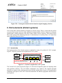
EXTRA ELEMENTS (VARIANT SYSTEMS) ............................................................................................................. 59
6.1 INTRODUCTION ........................................................................................................................................................ 59
6.2 AUXILIARY DATA ....................................................................................................................................................... 60
6.2.1
Auxiliary elements ...................................................................................................................................... 60
6.2.2
Technology forecasting .............................................................................................................................. 60
6.2.3
Option Volatility ......................................................................................................................................... 61
6.2.4
Component upgrade................................................................................................................................... 61
6.3 VARIANT DATA ......................................................................................................................................................... 62
6.3.1
Variant elements ........................................................................................................................................ 62
6.3.2
Technology forecasting .............................................................................................................................. 63
6.3.3
Option Volatility ......................................................................................................................................... 63
6.3.4
Component upgrade................................................................................................................................... 64
6.4 INTERFACE DATA ....................................................................................................................................................... 64
6.4.1
Interfaces.................................................................................................................................................... 64
6.4.2
Interface cost .............................................................................................................................................. 65
7.
EXTRA COMPUTATIONS (VARIANT SYSTEMS) ................................................................................................... 66
7.1 RULES..................................................................................................................................................................... 66
7.1.1
Components rules ....................................................................................................................................... 66
7.1.2
Interface rules............................................................................................................................................. 68
7.2 EXTRA EXCLUSIONS.................................................................................................................................................... 68
7.3 COMPUTATIONS ....................................................................................................................................................... 69
7.3.1
Single system .............................................................................................................................................. 69
7.3.2
Multi-system............................................................................................................................................... 72
7.4 ARCHITECTURE ......................................................................................................................................................... 75
Proprietary rights subject to title page
Page-5
AMISA
Contract: 262907
Number:
Revision:
Delivery ID:
Date:
Classification:
Dissemination level:
DFA902/110093
D3.5 Part-A
17.2.2014
Unclassified
PU
7.4.1
Single system .............................................................................................................................................. 75
7.4.2
Multi system ............................................................................................................................................... 76
7.5 ANALYSIS ................................................................................................................................................................ 77
7.5.1
Explore system architectures space............................................................................................................ 77
7.5.2
Conduct sensitivity analysis ........................................................................................................................ 77
8.
REPORTS ........................................................................................................................................................... 79
8.1
8.2
9.
DATABASE REPORTS .................................................................................................................................................. 79
CALCULATE REPORTS (NOT IMPLEMENTED) .................................................................................................................... 80
UTILITIES ........................................................................................................................................................... 80
9.1 DATABASE INTEGRITY................................................................................................................................................. 80
9.1.1
Procedure ................................................................................................................................................... 81
9.1.2
Example ...................................................................................................................................................... 81
9.2 BLACK-SCHOLES INVESTIGATION .................................................................................................................................. 81
9.2.1
Procedure ................................................................................................................................................... 82
9.2.2
Example ...................................................................................................................................................... 82
9.3 GENETIC ALGORITHM DEMONSTRATION ........................................................................................................................ 82
9.4 ACQUIRE EXTERNAL OPTION VALUES ............................................................................................................................ 83
Proprietary rights subject to title page
Page-6
AMISA
Number:
Revision:
Delivery ID:
Date:
Classification:
Dissemination level:
Contract: 262907
DFA902/110093
D3.5 Part-A
17.2.2014
Unclassified
PU
1. Introduction
1.1
DFA-Tool hardware and software
This section deals with the top level DFA-Tool hardware and software.
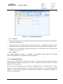
1.1.1
DFA-Tool – Top-level system
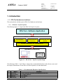
The following Figure 1-1 depicts the DFA-Tool top level system.
DFA-Tool - Software Application
Software infrastructure
Microsoft Office
Professional Plus 2010
Visual Studio 2010
Professional
Microsoft SQL Server
2008 R2
Windows-7 Professional x 64 - Operating System
Hardware infrastructure
Figure 1-1 – DFA-Tool – Top-level system design
The following Table 1-1 and Table 1-2 depict the recommended hardware and software (users and
developers) infrastructure for the DFA-Tool development, use and maintenance.
Table 1-1 - Recommended Hardware Specifications
#
1.
2.
3.
4.
Subject
Processor
Main Memory
Monitor
Hard Disk
Parameter
Core i5 Processor (for high speed optimization processes)
4 GB Main Memory
22" Monitor
500 GB
Proprietary rights subject to title page
Page-7
AMISA
Number:
Revision:
Delivery ID:
Date:
Classification:
Dissemination level:
Contract: 262907
DFA902/110093
D3.5 Part-A
17.2.2014
Unclassified
PU
Table 1-2 - Recommended Software Specifications
#
Subject
Software
1.
Operating system
2.
Database system
3.
4.
5.
Office software
Database application
Interface software
6.
Visual assist software
7.
Graphic software: (graph diagram)
8.
Graphic Software: (3-D surface)
9.
Debugger
10.
Source Control
1.1.2
Windows 7 Professional x 64 (English), Microsoft
Microsoft SQL Server 2008 R2 Express Edition,
Microsoft
Microsoft Office Professional Plus 2010, Microsoft
Visual Studio 2010 Professional, Microsoft
Telerik RadControls for WPF, Telerik
Visual Assist X v.10 for Visual Studio 2010, Whole
Tomato Software
Northwood.GoWPF, SKU: xamwpf, Northwoods
Software Corporation
TBD
EurekaLog.NET 6 Enterprise for Visual Studio,
EurekaLog
Subversion for Visual Studio ( Server/Client),
VISUALSVN
S/W
developer
X
X
X
X
X
X
X
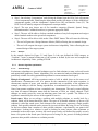
Notes - DFA-Tool hardware and software
1. The DFA-Tool is designed to be installed on a PC and run locally, as a standalone program.
The tool is not being supported in a client-server configuration.
2. The hardware table should be viewed as a recommendation in order to achieve fast
optimization processing. The Intel Core i3 is also an acceptable processor.
3. In order to accommodate users with older system versions, the DFA-Tool is written in a 32
Bit configuration. This means the tool is able to run under both 32 and 64 Bit systems but is
somewhat slower (a restriction to the optimization process which require high processing
speed). If funding allows, the tool will be regenerated also in a 64 Bit version.
4. The Microsoft SQL Server 2008 R2 Express Edition database system is available free of
charge.
5. According to the AMISA proposal and the AMISA consortium agreement, the DFA-tool
shall be free to all users and its software placed under open source licensing rules.
1.2
DFA-Tool operations and concepts
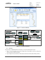
1.2.1
Operation scenario
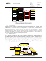
Figure 1-2 depicts a typical DFA-Tool operation scenario.
Proprietary rights subject to title page
Page-8
AMISA
Number:
Revision:
Delivery ID:
Date:
Classification:
Dissemination level:
Contract: 262907
Projects
DFA902/110093
D3.5 Part-A
17.2.2014
Unclassified
PU
Components data
Open
Static data
Reports
Manage
Extra
Computations
Computations
Help
Architecture
Database reports
Calculate reports
Rules
Exit
Dynamic structures
Utilities
Exclusions
Analysis
Data integrity
Project data
Computations
Data
Black-Scholes
Extra Elements
Architecture
Architecture
Auxiliary Data
GA Demo
Analysi
Static structures
Variant Data
Dynamic structures
Interface Data
External OVs
Figure 1-2 – DFA-Tool operation scenario
(Implemented functions are depicted in red)
1.2.2
Leaf components
The target system is composed of components organized in a hierarchical structure. We define “Leaf
components” as the set of the lowest level components in the system, which are of interest to a
particular system designer. Users of the DFA-Tool should note that computations of optimal
adaptable architecture consider only leaf components and other elements (e.g. interfaces) associated
with them. Other, higher level definitions, may be inserted into the database for the convenience of
the user but are totally ignored by the optimization software.
1.2.3
Database integrity
DFA-Tool users should be aware that, in order to insure the integrity of the database, deletions of
any database element can only be done hierarchically by removing the lowest elements first. The
DFA-Tool software will resist attempts to delete a database element which is attached to a lower
hierarchical level element. For example, a component having one or more son-component cannot be
deleted until all the attached son-components are deleted. Likewise, a component attached to one or
more interfaces cannot be deleted until all the attached interfaces are deleted. The hierarchical
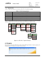
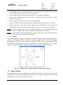
structure of the DFA-Tool database elements is depicted in Figure 1-3.
Project
Dynamic structures:
Static Structure:
- Options Param.
Environment
- Initial Value
- Value Desired
- System Value
- Upgrade Cost
Static Data:
- Tech. Forecasting
- Option Volatility
- Component Upgrade
- Interface Cost
Components
Exclusions
Interfaces
Interface cost
Auxiliary/Variant
Components
Auxiliary/Variant
Interfaces
Auxiliary/Variant
rules
Figure 1-3 – Hierarchical structure of the DFA-Tool database
Proprietary rights subject to title page
Page-9
AMISA
1.3
Number:
Revision:
Delivery ID:
Date:
Classification:
Dissemination level:
Contract: 262907
DFA902/110093
D3.5 Part-A
17.2.2014
Unclassified
PU
Top level view
Table 1-3 depicts the top two level elements of the DFA-Tool and their meaning.
Table 1-3 – DFA-Tool top elements
Name
Projects
Project Data
Component Data
Computations
Extra Elements
Extra Computations
Reports
Utilities
Meaning
Identify an active project, manage projects, help users and exit the DFA tool
Define project-wide input parameters
Define component-level and Interface-level input parameters
Compute the output of the DFA tool and perform sensitivity analysis
Define auxiliary and variant components/interfaces
Calculate / analyze variant systems with auxiliary and variant components/interfaces
Generate reports of the input parameters and output results
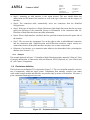
Provide various utilities
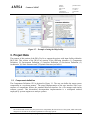
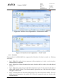
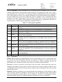
Figure 1-4 depicts the top two layers of the DFA-Tool Graphical User Interface (GUI). The meaning
of each is explained later in this document (Implemented functions are depicted in red).
Projects
Project Data
Open:
- Project-A
- Project-B
- ...
Components
Manage:
- Edit
- Replicate
- Export
- Import
Interfaces
Environment
Exclusions
Architecture
Computations
Extra Elements
Extra Computations
Rules:
Architecture
- DSM Generation
- Manual
- Optimization
- Optimize Architecture
Auxiliary Data:
Dynamic Structure:
- Value Loss
- Accum. Value Loss
- Upgrade Time
Variant Data:
Computations:
- Define elements
- Tech. Forecasting
- Option Volatility
- Components Upgrade
- Single system
- Multi system
Analysis:
- Sensitivity
Help
Exit
Component Data
Static Data:
- Tech. Forecasting
- Option Volatility
- Component upgrade
- Interface Cost
Static Structure:
- Options Param.
- Define elements
- Tech. Forecasting
- Option Volatility
- Components Upgrade
Interface Data:
- Interfaces
- Interface cost
- Components
- Interfaces
Exclusions:
- Extra
Architecture:
- Single system
- Multi system
Analysis:
- Single system
- Multi system
Dynamic Structure:
- Initial Value
- Value Desired
- System Value
- Upgrade Cost
Reports
Database report
Utilities
Data Integrity
Black-Scholes
Calculate report
Demo GA
Import External OVs
Figure 1-4 – DFA Tool – Top two GUI layers
2. Projects
The Projects section of the DFA-Tool consists of the following elements: (1) Open a project, (2)
Manage projects, (3) Help services and (4) exit (see below).
Proprietary rights subject to title page
Page-10
AMISA
2.1
Contract: 262907
Number:
Revision:
Delivery ID:
Date:
Classification:
Dissemination level:
DFA902/110093
D3.5 Part-A
17.2.2014
Unclassified
PU
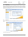
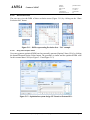
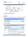
Open a project
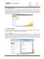
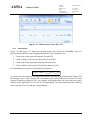
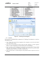
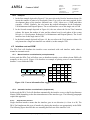
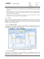
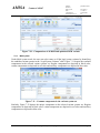
The Select a project GUI is depicted in Figure 2-1. The user can select any one of several defined
and independent “Projects” within the DFA-Tool database. The project named “UAV-Example” is a
general example, helping users understand the DFA-Tool. This project may be selected and
modified but the users cannot delete the project nor modify its name. The Appendix at the end of
this guide further describes this example.
Figure 2-1 – Open a project GUI
2.2
Manage projects
The user can manage the database projects by performing the following functions: (1) Edit project,
(2) Replicate project, (3) Export project and (4) Import project
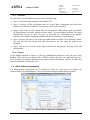
2.2.1
Edit project
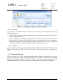
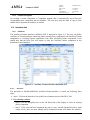
Figure 2-2 depicts the Edit project GUI. The user can modify the name of an existing project in the
database or delete an existing project from the database. This may be done by clicking on the
desired function (in this case: Edit) and then performing the required operation on the opened
window and. The user should note that valid project names may only be composed of the following
characters: “a-z”, “A-Z”, “0-9”, “-“, “_”.
Figure 2-2 – Edit Project GUI
Proprietary rights subject to title page
Page-11
AMISA
2.2.2
Contract: 262907
Number:
Revision:
Delivery ID:
Date:
Classification:
Dissemination level:
DFA902/110093
D3.5 Part-A
17.2.2014
Unclassified
PU
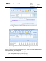
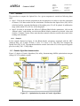
Replicate project
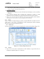
Figure 2-3 depicts the Replicate project GUI. Replicating a project is a process of copying the
database of an existing project and saving it under a new name. This may be done by clicking on the
desired function (in this case: Replicate) and then performing the required operation on the opened
window. The user should note that valid project names may only be composed of the following
characters: “a-z”, “A-Z”, “0-9”, “-“, “_”.
Figure 2-3 - Replicate Project GUI
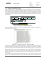
2.2.3
Export project
Generate an XML file from a Project in the database for external use (follow the simple wizard
steps).
Figure 2-4 – Export Project GUI
Typical XML file appears below
Proprietary rights subject to title page
Page-12
AMISA
Contract: 262907
Number:
Revision:
Delivery ID:
Date:
Classification:
Dissemination level:
DFA902/110093
D3.5 Part-A
17.2.2014
Unclassified
PU
Figure 2-5 – Partial XML example
2.2.4
Import project
Create a Project in the database from an existing external XML file (follow the simple wizard steps).
Figure 2-6 - Import Project GUI
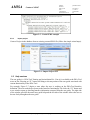
2.3
Help services
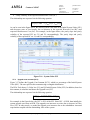
The user guide (i.e. DFA-Tool Training and Assimilation Kit – Part-A) is available to the DFA-Tool
users on line. Pressing an “F1” button will bring a relevant portion of the user guide associated with
current functionality of the DFA-Tool.
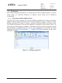
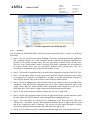
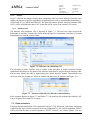
For example, Figure 2-7 depicts a state where the user is working on the DFA-Tool Interface
definition. The user needs help relevant to the Interface functionality. He clicks the “F1” button and
a new window opens up showing Interface information extracted from the user guide. The right side
of the window provides the actual user guide help and the left side of the window allows the user to
browse freely throughout the user guide.
Proprietary rights subject to title page
Page-13
AMISA
Contract: 262907
Number:
Revision:
Delivery ID:
Date:
Classification:
Dissemination level:
DFA902/110093
D3.5 Part-A
17.2.2014
Unclassified
PU
Figure 2-7 – Example of using the Help facility
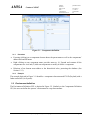
3. Project Data
The purpose of this portion of the DFA-Tool is to support the project-wide input facility within the
DFA-Tool. This section of the DFA-Tool consists of the following elements: (1) Components
Definition, (2) Environment Definition, (3) Interface Definition, (4) Exclusions Definition, (5)
Architecture, (6) Static Structure and (7) Dynamic Structure (see below).
3.1
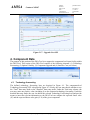
Components definition
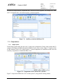
The Components Definition GUI is depicted in Figure 3-1. The user can define the target system
composition in a top-down manner1. The actual implementation of the user interface with a tree
structure of components follows the standard Microsoft interface for a file manager and similar
software systems. This hierarchical decomposition implementation is a widespread method
employed by systems engineers to analyze systems.
1
The reader should note that only the system leaves-components (the lowest leaves of the system, which interest the
designer) are relevant for the structural optimization of the target system.
Proprietary rights subject to title page
Page-14
AMISA
Contract: 262907
Number:
Revision:
Delivery ID:
Date:
Classification:
Dissemination level:
DFA902/110093
D3.5 Part-A
17.2.2014
Unclassified
PU
Figure 3-1 – Components definition
3.1.1
Procedure

Focusing (clicking) on a component element shows the parent name as well as the components’
abbreviated and full name.

Right clicking on any component name provides menu to: (1) Expand and contract all the
components tree-view and (2) Add son-components or modify or delete a component.

Deletions of an element must adhere to the hierarchical rules, protecting the database (See
Section 1.2.3).
3.1.2
Example
The example depicted in Figure 3-1 identifies a component element named PYLD (Payload) with a
father named AS (Air System).
3.2
Environment definition
The Environment Definition GUI is depicted in Figure 3-2. Similarly to the Components Definition
GUI, the user can define the systems’ environment in a top-down manner.
Proprietary rights subject to title page
Page-15
AMISA
Contract: 262907
Number:
Revision:
Delivery ID:
Date:
Classification:
Dissemination level:
DFA902/110093
D3.5 Part-A
17.2.2014
Unclassified
PU
Figure 3-2 – Environment Definition
3.2.1
Procedure

Focusing (clicking) on an environment element shows the parent name and the environments’
abbreviated and full name.

Right clicking on any environment name provides menu to: (1) Expand and contract all the
environment tree-view and (2) Add son-environment or modify or delete an environment name.

Deletions of an environment element must adhere to the hierarchical rules, protecting the
database (See Section 1.2.3).
3.2.2
Example
The example depicted in Figure 3-2 identifies an environment element named TAC-COMM
(Tactical Communication) with a father named Environment.
3.3
Interface definition
The Interface Definition GUI is depicted in Figure 3-3. The user can define interfaces between
different elements within the target system as well as interfaces between elements in the target
system and its environment.
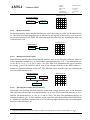
One of six types of interfaces may be defined: (1) Single-Direction, (2) Bi-Direction, (3) MultiDirection, (4) Split-OTM-Bi-Direction, (5) Split-MTO-Bi-Direction or (6) Split-Multi-Direction
(Figure 3-4). One of four categories of interfaces may be defined: (1) Material, (2) Spatial, (3)
Energy or (4) Information.
Proprietary rights subject to title page
Page-16
AMISA
Number:
Revision:
Delivery ID:
Date:
Classification:
Dissemination level:
Contract: 262907
DFA902/110093
D3.5 Part-A
17.2.2014
Unclassified
PU
Figure 3-3 – Interface definition
Multi-Dir Interface
Single-Dir Interface
Bi-Dir Interface
XXX
Component A
Component A
XXX
Component A
Component B
Component B
XXX
Component B
Component C
Split-Single-OTM Interface
Component A
Component B
XXX
Split-Single-MTO Interface
Component B
XXX
Component C
(Prime)
Component C
Component A
(Prime)
Env
Env
Split-Bi-Dir Interface
Component B
XXX
Component A
Component C
(Prime)
Env
Figure 3-4 – Six types of interfaces
3.3.1
Procedure
The procedure to Add/Modify/Delete an interface is carried out following these steps:

Step-1: Use the Navigation tree on the left hand side of the display to select an element for
which an interface should be defined.

Step-2: Right click on the Interface Table and select the desired action (Add, Modify, Delete)
Proprietary rights subject to title page
Page-17
AMISA
Contract: 262907
Number:
Revision:
Delivery ID:
Date:
Classification:
Dissemination level:
DFA902/110093
D3.5 Part-A
17.2.2014
Unclassified
PU

Step-3: Assuming an Add interface is the action desired. The user should define the
abbreviation and full name of the interface as well as the type of interface and the category of
interface.

Step-4: The connection table, automatically select one connection from the identified
Navigation tree.

Step-5: If the type of interface is a Single-Direction or Split Single-Direction, then the user must
specify the direction of the connection (Source or Destination) in the connection table. BiDirection or Multi-Direction do not need this information.

Step-6: When a Split interface is defined, the first specified element becomes the prime side of
the interface.

Step-7: The user uses the Assignment Tree on the right in order to add additional connection
into the connection table. Single-Direction and Bi-Direction interfaces require exactly two
connections whereas all the other interfaces may have two or more connections.

Deletions of an interface or a connection must adhere to the hierarchical rules, protecting the
database (See Section 1.2.3).
3.3.2
Example
The example depicted in Figure 3-3 identifies a Multi-Direction interface named AV-Bus (AV-Bus)
of category Information. It connects the AM (Air-Mission), PYLD (Payload), AV (Air-Vehicle) and
AC (Air-Comm.) Components.
3.4
Exclusions definition
The Exclusion sets definition GUI is depicted in Figure 3-5. The user can define mutually exclusive
sets of components, within the target system. Components from mutually exclusive sets cannot
reside within a single module and therefore, may interact only by means of an interface. Of course, a
given component cannot appear in two sets.
Figure 3-5 – Exclusions definition
Proprietary rights subject to title page
Page-18
AMISA
3.4.1
Contract: 262907
Number:
Revision:
Delivery ID:
Date:
Classification:
Dissemination level:
DFA902/110093
D3.5 Part-A
17.2.2014
Unclassified
PU
Procedure
The procedure to Add/Modify/Delete an Exclusion set is carried out following these steps:

Step-1: Right click on the Exclusion Table and select the desired action (Add, Modify, Delete).

Step-2: Assuming an Add Exclusion set is the action desired. The user should firstly define the
name of the exclusion set.

Step-3: Next, the user clicks on the Components Sets table and then clicks on a selected
component from the assignment Tree in order to add it into the Exclusion set.

Step-4: This process (Step-3 alone or Step-1 to Step-3) may be repeated as needed.
3.4.2
Example
The example depicted in Figure 3-5 identifies four exclusive sets of components within an
Unmanned Air Vehicle (UAV) System. The three Exclusive sets are: (1) the Air Vehicle system, (2)
Ground communication, (3) Remote Terminal and (4) Other system components. In particular, the
Remote Terminal System set is composed of the following components: RT-REC (RT Receiver),
RT-DIS (RT Display) and RT-CON (RT Control).
3.5
Architecture
The user can generate graphical charts of the project architecture.
3.5.1
Procedure
The procedure to generate graphical charts of the project architecture is done following these steps:

Step-1: Select the desired interface category. If the system is complex and contains multiinterface types, the users should generate architecture charts for each type of interface.

Step-2: If an architecture chart is saved from a previous session then the user can show it by
clicking the “Show” button. Note that saved architecture charts may not be valid if relevant
database parameters have been modified.

Step-3: Click on the “Build” button. The raw architecture will be displayed (Often a maximal
window is preferable). The detail of each architecture chart is depicted in the blue strip just
above the chart.

Step-4: The user can edit the architecture chart by identifying and moving individual or groups
of symbols of components, environments or splitting points of interfaces.

Step-5: The user can “Save” the edited chart and later “Show” a saved architecture chart by
clicking the relevant buttons.

Step-6: Also the user can change the “Scale” of the image using the slide at the bottom-left.
Proprietary rights subject to title page
Page-19
AMISA

DFA902/110093
D3.5 Part-A
17.2.2014
Unclassified
PU
Step-7: The user can select an object (i.e. Components, Environment or Interface) and click on
the “Parameter” tab. A window will slide open revealing the parameters associated with the
selected object.
3.5.2

Contract: 262907
Number:
Revision:
Delivery ID:
Date:
Classification:
Dissemination level:
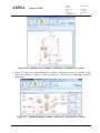
Example
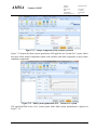
Figure 3-6 depicts a “Raw”, “Combined” architecture of the UAV system.
Figure 3-6 – Raw “Combined” architecture - UAV system

Figure 3-7 depicts the edited “Information” architecture of the UAV system. Note the
“unconnected” components or interfaces in each view.
Figure 3-7 - Edited “Information” architecture - UAV system
Proprietary rights subject to title page
Page-20
AMISA

Contract: 262907
Number:
Revision:
Delivery ID:
Date:
Classification:
Dissemination level:
DFA902/110093
D3.5 Part-A
17.2.2014
Unclassified
PU
Figure 3-8 depicts the same information. Here, a component is selected and the “Parameters”
window is open revealing the parameters associated with the selected component.
Figure 3-8 – Component and parameter information window

Figure 3-9 depicts the corresponding edited “Energy” architecture. Note the “unconnected”
components or interfaces in each view.
Figure 3-9 - Edited “Energy” architecture - UAV system
3.6
Static Structure / Option Default Parameters
The context of the Option Default Parameters is depicted in Figure 3-10. The actual user GUI is
depicted in Figure 3-11. The user can define the following project-level defaults: (1) Time [Years]
to update the system and (2) Risk-free interest rate [%] for updating the target system. These two
parameters are used in the Black-Scholes Options Value (OV) equation.
Proprietary rights subject to title page
Page-21
AMISA
Number:
Revision:
Delivery ID:
Date:
Classification:
Dissemination level:
Contract: 262907
DFA902/110093
D3.5 Part-A
17.2.2014
Unclassified
PU
Project Data
Static Structures
Option
Parameters
Step-1: define project-wide default parameters for the
Black-Scholes Options Value (OV) equation
Black-Scholes Equation:
Tailoring
Component
current value
Model - A
Option default parameters
Value
Time to upgrade [Years]
5.0
Risk-free interest rate [%]
2.5
Risk-free
interest rate
Component
Upgrade cost
Time to
upgrade
OP  S * N (d1 )  X * e rT *(d1  V * T )
Standard
normal
distribution
d1 
σ2 
S  
ln     r 
T
2 
X 
 T
Volatility
(Standard deviation of
potential future value
distribution)
Figure 3-10 – Context of the Options Default Parameter
Figure 3-11 - Options default parameter GUI layout
3.6.1
Procedure
The procedure to define a project-level Options Default Parameters is carried out as follows:
Right click on any of the two default parameters (i.e. Time to upgrade, Risk-free interest rate) and
define the relevant parameters. For each parameter, the user should insert three records: (1) a
Minimum, (2) a Most likely and (3) a Maximum values. Such three valued sets are essentially,
triangular distributions of estimated values. The DFA-Tool computes each center of gravity of these
imaginary triangles which constitute the appropriate parameters for the Black-Scholes Options Price
(OP) equation.
3.6.2
Example
The example depicted in Figure 3-11 identifies a Time to upgrade data set of: MIN=ML=MIN=5
years, and the final computed parameter is 5 years. Similarly, the Risk-free interest rate set is given
as: MIN=2.0%, ML=2.5% and MAX=3.0% with a final computed parameter of 2.5%.
3.7
Dynamic Structure
The Dynamic modeling of system lifecycle value and value-loss is depicted in Figure 3-12.
Essentially all system provides value to stakeholders. This value starts at an Initial system Value
(ISV). However, the value of systems tends to diminish due to: (1) Hardware and software Wear-out
Proprietary rights subject to title page
Page-22
AMISA
Number:
Revision:
Delivery ID:
Date:
Classification:
Dissemination level:
Contract: 262907
DFA902/110093
D3.5 Part-A
17.2.2014
Unclassified
PU
Costs (WC) and (2) Components & infrastructure Obsolescence Costs (OC). At the same time,
stakeholders tend to desire improved systems over time. This is mostly due to: (1) Expected
Economic Growth (EG) and (2) Technological Advances (TA). Our purpose in the dynamic
structure portion of the DFA-Tool to determine optimal upgrade time of the system.
Value[€]
Value Loss
Value Desired by Stakeholders
Accumulated Value Loss
Initial
system
value
System
upgrade
p
lue m
Va yste
e
s
m
eti by
Lif ded
i
rov
System
diminishing
value
Time
Figure 3-12 – System value and value loss
The following subsections describe the essential data required in order to estimate the optimal
upgrade time of the system: (1) Initial system value, (2) Value desired, (3) System value and (4)
Upgrade cost
3.7.1
Initial system value
Figure 3-13 depicts initial values needed for, eventually, estimate the system upgrade time. This
includes two aspects:
1. Definitions of the relevant time-horizon.
The user can specify the units (Months or Years) and their number. The allowable range of Months
or Years is 0-150. For example, in the figure below, the selected time-horizon is 10 Years.
2. Definitions of the Initial System Value (ISV).
The user can specify the Initial System Value (ISV) using a triangular distribution. For example, in
the figure below the ISV is defined as €130M (Minimum=€100M, Most likely=€110M and
Maximum=€180M)
Proprietary rights subject to title page
Page-23
AMISA
Contract: 262907
Number:
Revision:
Delivery ID:
Date:
Classification:
Dissemination level:
DFA902/110093
D3.5 Part-A
17.2.2014
Unclassified
PU
Figure 3-13 – Initial System Value (ISV) GUI
3.7.2
Value desired
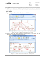
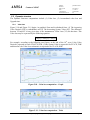
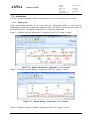
Figure 3-14 and Figure 3-15 depict the expected system value desired by stakeholders. The user
specifies four parameters using a triangular distribution. These parameters are:
1. Yearly slope of the expected Economic Growth (EG)
2. Yearly volatility of the expected Economic Growth (EG)
3. Yearly slope of the expected Technology Advances (TA)
4. Yearly volatility of the expected Technology Advances (TA)
The relationships are expressed via the following equation:
VD(t )  ISV  f EG (t )  fTA (t )
As can be seen in the figure below, the desired system value starts at the Initial System Value (ISV)
and increases, more or less linearly, due to increases in the expected Economic Growth (EG) and
expected Technology Advances (TA). For example, in the figure below, the yearly slope and yearly
volatility of the expected EG are 1% and 5% correspondingly. The yearly slope and yearly volatility
of the expected TA are 3% and 8% correspondingly.
Proprietary rights subject to title page
Page-24
AMISA
Contract: 262907
Number:
Revision:
Delivery ID:
Date:
Classification:
Dissemination level:
DFA902/110093
D3.5 Part-A
17.2.2014
Unclassified
PU
Figure 3-14 – Value Desired GUI – Graph representation
Figure 3-15 - Value Desired GUI – Table representation
3.7.3
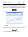
System value
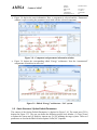
Figure 3-16 depicts the expected system value over time. The user specifies four parameters using a
triangular distribution. These parameters are:
1. Yearly slope of the expected Wear-out Cost (WC)
2. Yearly volatility of the expected Wear-out Cost (WC)
3. Yearly slope of the expected Obsolescence Cost (OC)
Proprietary rights subject to title page
Page-25
AMISA
Contract: 262907
Number:
Revision:
Delivery ID:
Date:
Classification:
Dissemination level:
DFA902/110093
D3.5 Part-A
17.2.2014
Unclassified
PU
4. Yearly volatility of the expected Obsolescence Cost (OC)
The relationships are expressed via the following equation:
SV (t )  ISV   fWC (t )  fOC (t ) 
As can be seen in the figure below, the desired system value starts at the Initial System Value (ISV)
and decreases, more or less linearly, due to increases in the expected Wear-out Cost (WC) and
expected Obsolescence Cost (OC). For example, in the figure below, the yearly slope and yearly
volatility of the expected WC are 3% and 5% correspondingly. The yearly slope and yearly
volatility of the expected OC are 1% and 8% correspondingly.
Figure 3-16 – System Value GUI
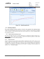
3.7.4
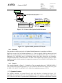
Upgrade cost constant (UCC)
Figure 3-17 defines the Upgrade Coat Constant (UCC), which is a percentage of the Initial System
Value (ISV). The user specifies this constant using a triangular distribution.
The DFA-Tool shows (1) Value loss (VL) and (2) Initial System Value (ISV). In addition, based on
this constant, it calculates and shows the Upgrade cost (UC).
The relationships are expressed via the following equation:
UC (t )  UCC * ISV  VL(t )
For example, in the figure below, the UCC is 50% of the ISV. Since ISV = €130K, then initially the
system upgrade cost starts at €65K. This upgrade cost increases over time due to increase in Value
Loss (VL). In other words, we model the upgrade cost increases due to the stakeholders increased
expectations coupled with the diminishing value of the system.
Proprietary rights subject to title page
Page-26
AMISA
Contract: 262907
Number:
Revision:
Delivery ID:
Date:
Classification:
Dissemination level:
DFA902/110093
D3.5 Part-A
17.2.2014
Unclassified
PU
Figure 3-17 – Upgrade Cost GUI
4. Component Data
The purpose of this portion of the DFA-Tool is to support the component-level input facility within
the DFA-Tool. This section of the DFA-Tool consists of the following elements: (1) Technology
Forecasting, (2) Option Volatility, (3) Component Upgrade and (4) Interface Cost (see below).
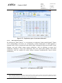
4.1
Technology forecasting
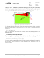
The defined technology forecasting laws are depicted in Figure 4-1. The component-level
Technology Forecasting GUI is depicted in Figure 4-2. Firstly, the user must decide whether to use
the “Total” data entry mode or the “Detailed” data entry mode. Under the Total entry scheme, the
user may enter one positive value (including 0) as the estimated technology forecasting. Under the
detailed data entry mode, the user can define the selected Technology Forecasting laws and provide
means to insert the relevant information so the DFA-Tool can compute the expected future value
(S’) and the expected future value gain (S’-S) of the given component.
Proprietary rights subject to title page
Page-27
AMISA
Contract: 262907
Number:
Revision:
Delivery ID:
Date:
Classification:
Dissemination level:
DFA902/110093
D3.5 Part-A
17.2.2014
Unclassified
PU
Figure 4-1 – Defined technology forecasting laws
Figure 4-2 – Technology Forecasting data
4.1.1
Procedure
The procedure to Add/Modify/Delete component-level Technology Forecasting data is carried out
following these steps:

Step-1: Right click on the relevant component in the navigation tree and select the desired
action (Add, Modify, Delete).

Step-2: The user must define the model of data entry either “Detailed” (as will be explained
below) or “Total” in which the user can enter directly any value (including 0)

Step-3: Assuming an add Technology Forecasting data is the action desired. The user should
firstly add a new entry in the Technology Forecasting Table. Also the user can ask for more
information related to TRIZ rules on systems evolutionary laws.

Step-4: Insert the name or a short description of the parameter which is expected to evolve in
the future.
Proprietary rights subject to title page
Page-28
AMISA
Contract: 262907
Number:
Revision:
Delivery ID:
Date:
Classification:
Dissemination level:
DFA902/110093
D3.5 Part-A
17.2.2014
Unclassified
PU

Step-5: Right-click on up to three forecasting laws, identifying the forecasting law(s) which are
expected to govern the evolution of the relevant parameter.

Step-6: Identify the initial and the expected final level of component technology.

Step-7: Insert a weight factor for each parameter. The DFA-Tool expects the sum of all the
weights to be equal 1.00.

Step-8: Continue this process (Step-2 to Step-6) appropriately.

Step-9: The DFA-Tool will compute the derived multiplications and sums (∑Ii*Wi ; ∑Fi*Wi).

Step-10: Insert the current value of the component and the DFA-Tool will calculate the
expected future value (S’) and the expected future value gain (S’-S) of the given component.
Note-1:
The user can place the cursor on the different identifiers of the Technology Forecasting
Laws (1-21) and the DFA-Tool will display the relevant names of the laws.
Note-2:
If the number of forecasting parameters exceeds two, the user can ask for a Radar chart in
order to visualize the expected technical gains.
4.1.2
Example
The example depicted in Figure 4-2 identifies six parameters affecting future technology advances
relevant to the Payload (PYLD) of the UAV system, together with its relevant Technology
Forecasting laws (See Figure 4-1). Based on the data in the table and the current component value
S=€450K, the expected future value of the component is S’= €796K and the gain is S’-S= €346K.
Figure 4-3 depicts a Radar chart of initial, expected and final component-levels technology.
Figure 4-3 – Radar chart – Future component technology prediction
4.2
Option Volatility
The component-level Option Volatility value is depicted in Figure 4-4. The user can insert the
volatility factor of the given component so the DFA-Tool can compute the Option Value (OV) and
the distribution of the expected component’s results.
Proprietary rights subject to title page
Page-29
AMISA
Contract: 262907
Number:
Revision:
Delivery ID:
Date:
Classification:
Dissemination level:
DFA902/110093
D3.5 Part-A
17.2.2014
Unclassified
PU
Figure 4-4 - Components’ Option Volatility GUI layout
4.2.1
Procedure
The procedure to Add/Modify/Delete a component-level Technology Forecasting data is carried out
following these steps:

Step-1: Right click on the relevant component in the navigation tree and select the desired
action (Add, Modify, Delete).

Step-2: Assuming an add Option Volatility data is the action desired. The user should insert
three records: (1) a Minim, (2) a Most likely and (3) a Maximum values. This is essentially a
triangular distribution of estimated Option Volatility values. The DFA-Tool will compute the
center of gravity of this imaginary triangle which is the representative result.
4.2.2
Example
The example depicted in Figure 4-4 identifies an Option Volatility data set of the PYLD (Payload):
MIN=10%, ML=15% and MAX=20%. The final value of the Option Volatility is calculated to be
15%.
4.3
Component Upgrade
The user can use one of two Component Upgrade insertion schemes. Accordingly, the user may
employ the Component Upgrade cost depicted in Figure 4-5 (“Detailed” scheme) or the Component
Upgrade cost depicted in Figure 4-6 (“Total” scheme). The user will then insert the relevant
information and the DFA-Tool will compute the overall upgrade cost for the given component.
Proprietary rights subject to title page
Page-30
AMISA
Contract: 262907
Number:
Revision:
Delivery ID:
Date:
Classification:
Dissemination level:
DFA902/110093
D3.5 Part-A
17.2.2014
Unclassified
PU
Figure 4-5 – Component upgrade cost computation – Detailed
Figure 4-6 – Component upgrade Cost computation - Total
4.3.1
Procedure
The following procedure defines the manner for defining upgrade cost insertion in a detailed way:

Step-1: Right click on the relevant component in the navigation tree.

Step-2: In the upgrade model box select radio button “Detailed”.

Step-3: Right click to add Component Upgrade Entry.

Step-4: Select tab “Materials”.

Step-5: Right click to add Detailed Component Upgrade Entry

Step-6: Add text describing the upgrade expenditure
Proprietary rights subject to title page
Page-31
AMISA
Contract: 262907
Number:
Revision:
Delivery ID:
Date:
Classification:
Dissemination level:
DFA902/110093
D3.5 Part-A
17.2.2014
Unclassified
PU

Step-7: If this not a Non-Recurring (NRE) expenditure, insert the relevant unit cost

Step-8: If this Non-Recurring (NRE) expenditure, identify it in the checkbox and then define the
NRE cost and the number of units for which this NRE cost is applicable.

Step-9: Repeat steps 3-8 for the “labor” tab and the “Other” tab.

The DFA-Tool will compute the center of gravity of this imaginary triangle which is the
representative result.
4.3.2
Examples
The example depicted in Figure 4-5 identifies a component Upgrade Cost data set of the Payload
(PYLD) in a “Detailed” configuration. The Materials, Labor and Other costs are €65K, €75K and
€90K respectively, for a total of €230K. The “material” cost is composed of NRE cost of €30K
divided into 2 PYLD units plus RE cost of €50K.
The example depicted in Figure 4-6 identifies a component Upgrade Cost data set of the Air Vehicle
(AV) in a “Direct” configuration. The estimated upgrade cost is MIN=€300K, ML=400K€ and
MAX=430K€. The final value of the upgrade cost is calculated to be €376K.
4.4
Interface Cost computations
The user can use one of three Interface Cost insertion schemes. Accordingly, the component-level
Interface Cost is depicted in Figure 4-7 (“Detailed” scheme), Figure 4-8 (“Partial-total” scheme) and
Figure 4-9 (“Total” scheme). The user then inserts the relevant information and the DFA-Tool will
compute the overall Interface Cost (IC) of the given interface.
Figure 4-7 – Interface Cost Computations – “Detailed” model
Proprietary rights subject to title page
Page-32
AMISA
Contract: 262907
Number:
Revision:
Delivery ID:
Date:
Classification:
Dissemination level:
DFA902/110093
D3.5 Part-A
17.2.2014
Unclassified
PU
Figure 4-8 - Interface Cost Computations – “Partial-total” model
Figure 4-9 - Interface Cost Computations – “Total” model
4.4.1
Procedure
The procedure to Add/Modify/Delete component-level Interface Cost data is carried out following
these steps:

Step-1: Right click on the relevant component in the navigation tree in order to select interface
connected to this component.

Step-2: Right click on the relevant interface in the Interface table in order to select the desired
interface.

Step-3: Right click on the desired model (Detailed, Partial total or Total) and select the desired
action (Add, Modify, Delete). The relevant model, depicted in one of the above three figures
will appear on the screen.

Step-4: Assuming the user selects the add Interface Cost data as the action desired. The user
should insert the appropriate data and the DFA-Tool will compute the unit cost related to the
selected interface.
Proprietary rights subject to title page
Page-33
AMISA
4.4.2
Number:
Revision:
Delivery ID:
Date:
Classification:
Dissemination level:
Contract: 262907
DFA902/110093
D3.5 Part-A
17.2.2014
Unclassified
PU
Examples
1. In the first example depicted in Figure 4-7, the user selects the Detailed insertion scheme. He
inserts the number of units to be developed (Units=2) as well as unit costs required for the
development phase of the interface (Material cost = €5K, Labor cost = €500K and Other
expenses = €20K). Similarly, the user inserts the needed information for the Production,
Use/Maintenance and Disposal phases. The overall interface cost of this single unit is €36K
2. In the Second example depicted in Figure 4-8, the user selects the Partial Total insertion
scheme. He inserts the number of units and the subtotal cost for each phase of the system
lifecycle (i.e. Development, Production, Use/Maintenance and Disposal phases). The overall
interface cost of this single unit is €35K.
3. In the third example depicted in Figure 4-9, the user selects the Total insertion scheme. He
only inserts the a single unit interface cost which is, in this example €35K
4.5
Interface cost and DSM
The DFA-Tool will distribute the interface costs associated with each interface under either a
manual or automatic mode.
4.5.1
Manual interface cost distribution (not implemented)
In this mode the DFA-Tool will allow users to distribute interface cost within relevant DSM cells
manually as they see fit. Figure 4-10 describes an example of placing costs of uneven interface
dataflow / costs within the DSM.
Radar
Antena
Radar
Antena
Radar
Antena
Radar
Processor
Radar
Control
Interface Cost = 200
Radar
Display
Radar
Processor
Radar
Display
10
50
Env
90
Radar
Processor
Radar
Control
Radar
Control
10
Radar
Display
20
10
10
Env
Figure 4-10 – Uneven information flow suggests uneven interface cost distribution
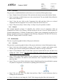
4.5.2
Automatic interface cost distribution (implemented)
In this mode the DFA-Tool will distribute automatically the interface cost over the Design Structure
Matrix (DSM) depending on the direction and nature of the interface type. The following paragraphs
explain this approach.
4.5.2.1
Single direction interface
Single direction interface means that the interface goes in one direction (i.e. from A to B). The
DFA-Tool implements this type of interface by placing the interface cost appropriately in the DSM.
The following figure describes this case assuming the total cost of the interface is 60.
Proprietary rights subject to title page
Page-34
AMISA
Number:
Revision:
Delivery ID:
Date:
Classification:
Dissemination level:
Contract: 262907
DFA902/110093
D3.5 Part-A
17.2.2014
Unclassified
PU
Interface Cost = 60
Single-Dir Interface
A
XXX
Component A
B
A
C
Env
60
Component B
B
C
Env
4.5.2.2
Bi-direction interface
Bi-direction interface means that the interface goes in two directions (i.e. from A to B and from B to
A). The DFA-Tool implements this type of interface by placing half of the interface cost in each of
the relevant locations of the DSM. The following figure describes this case assuming the total cost
of the interface is 60.
Interface Cost = 60
Bi-Dir Interface
A
XXX
Component A
B
A
C
Env
30
Component B
B
30
C
Env
4.5.2.3
Multi-direction interface (Bus)
Multi-direction interface (Bus) means that the interface goes in two directions within the entire set
of the connected elements (e.g. in a set of three connected elements, A, B, C, the interactions are:
A=>B, B=>A, A=>C, C=>A, B=>C and C=>B). The DFA-Tool implements this type of interface
by placing 1 (2n) of the interface cost in each of the relevant locations of the DSM (where n =
number of connected elements in the set)2. The following figure describes this case assuming the
total cost of the interface is 60.
Multi-Dir Interface
Interface Cost = 60
A
Component A
A
XXX
Component C
4.5.2.4
B
C
10
10
Env
Component B
B
10
C
10
10
10
Env
Split single One-To-Many direction interface
Split single One-To-Many direction interface means that a single interface goes in one direction
from one source (Prime) into several destinations (e.g. in a set of four connected elements, A, B, C
and Env, the interactions are: A =>B, A=>C and A=>Env). The DFA-Tool implements this type of
interface by placing 1 (n  1) of the interface cost in each of the relevant locations of the DSM (where
n = number of connected elements in the set). The following figure describes this case assuming the
total cost of the interface is 60.
2
Special cost distribution occurs when only two elements are interfaced via a Bus. In such situation: n  1 2 .
Proprietary rights subject to title page
Page-35
AMISA
Number:
Revision:
Delivery ID:
Date:
Classification:
Dissemination level:
Contract: 262907
DFA902/110093
D3.5 Part-A
17.2.2014
Unclassified
PU
Interface Cost = 60
A
Split-Single-OTM Interface
Component A
B
C
Env
20
20
20
Component B
XXX
A
Component C
(Prime)
B
C
Env
Env
4.5.2.5
Split single Many-To-One direction interface
Split single Many-To-One direction interface means that several interfaces go in one direction from
several sources into a single (Prime) destination (e.g. in a set of four connected elements, A, B, C
and Env, the interactions are: B =>A, C=>A and Env=>A). The DFA-Tool implements this type of
interface by placing 1 (n  1) of the interface cost in each of the relevant locations of the DSM (where
n = number of connected elements in the set). The following figure describes this case assuming the
total cost of the interface is 60.
Split-Single-MTO Interface
A
B
C
Env
Component B
XXX
A
Component C
Component A
B
20
C
20
Env
20
(Prime)
Env
4.5.2.6
Split Bi Direction interface
Split Bi Direction interface means that the interface goes in two directions from one source (Prime)
into several destinations and back (e.g. in a set of four connected elements, A, B, C and Env, the
interactions are: A=>B, B=>A, A=>C, C=>A, A=>Env and Env=>A). The DFA-Tool implements
this type of interface by placing 1 (2(n  1)) of the interface cost in each of the relevant locations of
the DSM (where n = number of connected elements in the set). The following figure describes this
case assuming the total cost of the interface is 60.
Split-Bi-Dir Interface
Interface Cost = 60
A
XXX
B
C
Env
10
10
10
Component B
A
Component A
(Prime)
Component C
B
10
C
10
Env
10
Env
5. Computations
The purpose of this portion of the DFA-Tool is to support the following computation facilities: (1)
Architecture, (2) Dynamic structure and (3) Sensitivity analysis (see below).
Proprietary rights subject to title page
Page-36
AMISA
5.1
Contract: 262907
Number:
Revision:
Delivery ID:
Date:
Classification:
Dissemination level:
DFA902/110093
D3.5 Part-A
17.2.2014
Unclassified
PU
Architecture
Deal with the following functionalities: (1) Design Structure Matrix (DSM) generation, (2) Manual
system design (3) Constraints definition, (4) Optimize system design and (5) Bottom-up
recombination.
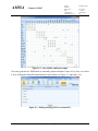
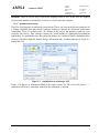
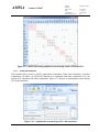
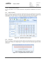
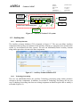
5.1.1
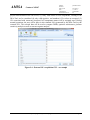
Design Structure Matrix (DSM) generation
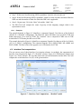
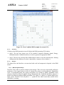
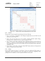
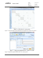
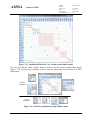
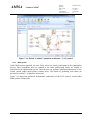
The DFA-Tool is able to generate five variants of DSMs, depending on the category of interface
(Material, Spatial, Energy, Information and a Combined interfaces). Figure 5-1 depicts the ManMachine interaction GUI. Figure 5-2 depicts a generated Information-DSM of the target system.
This includes identification of all the leaf-components, computation of their option values to be
placed along the DSM diagonal. In addition, all Information-category interfaces associated with the
leaf-components are identified and their costs are placed appropriately in the DSM. The reader
should note that the DFA-Tool will place a “--“ symbol in cells where certain data, needed for the
calculation, is missing.
Figure 5-1 – DSM generating GUI
Proprietary rights subject to title page
Page-37
AMISA
Contract: 262907
Number:
Revision:
Delivery ID:
Date:
Classification:
Dissemination level:
DFA902/110093
D3.5 Part-A
17.2.2014
Unclassified
PU
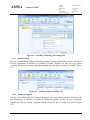
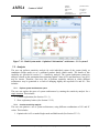
Figure 5-2 – Raw DSM Combined example
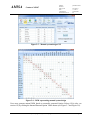
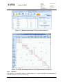
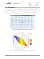
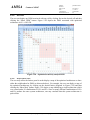
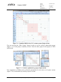
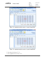
Users may generate raw DSM based on externally generated Option Values (OVs) (also, see section
9.4) by clicking the Internal/External Option Values button (see Figure 5-3 and Figure 5-4).
Figure 5-3 - DSM generating GUI for external OVs
Proprietary rights subject to title page
Page-38
AMISA
Contract: 262907
Number:
Revision:
Delivery ID:
Date:
Classification:
Dissemination level:
DFA902/110093
D3.5 Part-A
17.2.2014
Unclassified
PU
Figure 5-4 - Raw Combined DSM example for external OVs
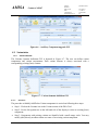
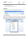
5.1.1.1
Procedure
Clicking on the DSM generation icon will display the DSM generating GUI window.

Step-1: The user may choose one of five interface categories (Material, Spatial, Energy,
Information and a Combined interfaces) in order to generate an appropriate DSM

Step-2: The user may click the Show DSM button in order to create the desired matrix. Missing
information in the database (if exists) is depicted by a sequence of two dashes (--).
5.1.1.2
Example
The Option Price and Interface cost associated with each leaf-component is depicted in the DSM
matrix.
5.1.2
Manual system design
The DFA-Tool is able to generate manual system designs. That is, the user can manually define the
architecture of the target system in order to compute the system overall Architecture Adaptability
Value. As mentioned before, the system can produce five variants of DSMs, dependent on the
category of interface (Material, Spatial, Energy, Information and a Combined interfaces). Figure 5-5
depicts this Manual combined DSM generation GUI. Figure 5-6 depicts a Combine-DSM of the
target system. The DFA-Tool will place a “--“ symbol in cells where certain data, needed for the
calculation, is missing.
Proprietary rights subject to title page
Page-39
AMISA
Contract: 262907
Number:
Revision:
Delivery ID:
Date:
Classification:
Dissemination level:
DFA902/110093
D3.5 Part-A
17.2.2014
Unclassified
PU
Figure 5-5 – Manual system design GUI
Figure 5-6 – DSM representing manual system design
Users may generate manual DSM based on externally generated Option Values (OVs) (also, see
section 9.4) by clicking the Internal/External Option Values button (see Figure 5-7 and Figure 5-8).
Proprietary rights subject to title page
Page-40
AMISA
Contract: 262907
Number:
Revision:
Delivery ID:
Date:
Classification:
Dissemination level:
DFA902/110093
D3.5 Part-A
17.2.2014
Unclassified
PU
Figure 5-7 - Manual system design GUI based on External OVs
Figure 5-8 - DSM representing manual system design based on External OVs
5.1.2.1
Procedure
The procedure to manually create a system design (i.e. assign individual leaf-components to
individual modules) involves the following:
Proprietary rights subject to title page
Page-41
AMISA
Contract: 262907
Number:
Revision:
Delivery ID:
Date:
Classification:
Dissemination level:
DFA902/110093
D3.5 Part-A
17.2.2014
Unclassified
PU

Step-1: On selecting “Computations” and clicking the Manual icon, the DFA-Tool will generate
a Leaf-components table, identifying the abbreviated and the full names of all the defined leafcomponents together with the components’ Option Price (OP) and Interface Costs (IC). The
DFA-Tool will initially assign each component to a unique module.

Step-2: The user may choose one of five interface categories (Material, Spatial, Energy,
Information and a Combined interfaces) to generate appropriate DSM.

Step-3: The user will be able to click on a module numbers of any leaf-component and assign a
desired module number to the given leaf-component.

Step-4: The user will be able to click on the “Show DSM” button. This will cause the following:
o The tool will generate a Design Structure Matrix (DSM) reflecting the user manual design.
o The tool will compute the target system Architecture Adaptability Value reflecting the user
manual design of the target system.
5.1.2.2
Example
In the example depicted in Figure 5-5 and Figure 5-6 the user defined the DSM category as
“Combine”, creates a manual architecture of the system as defined by the user and computes the
Architecture Adaptability Value, yielding €328.9K.
5.1.3
5.1.3.1
Genetic Algorithm optimization
GA methodology
Evolutionary algorithms are powerful techniques used to find solutions to many real-world search
and optimization problems. Genetic Algorithms (GA) are numerical analysis techniques that seem
particularly suitable for solving optimization problems in a non-continues search space.
Biological background. All living organisms consist of cells in which, there are the same set of
chromosomes. Chromosomes serve as a pattern for the construction of the entire organism. A
chromosome consists of genes, each encodes a particular trait or capability of the organism for
example, the ability to run fast. During reproduction, a recombination (or crossover) first occurs.
Genes from parents combine to form a completely new chromosome. The newly created offspring
may then be mutated. Mutation means that the elements of DNA are slightly changed. These
changes are mainly caused by errors in inheriting genes from one’s parents. The fitness of an
organism is measured by the success of the organism to survive.
Search space. When we are solving a problem with multiple solutions, we usually look for a
solution, which will be better than all the others. The space of all feasible solutions e.g. the set of all
solutions is called the search space. Each element in the search space represents a single possible
solution. Each possible solution can be assessed by its survival fitness. By using GA we are looking
for the best solution from a number of other possible solutions - represented by one point in the
search space. Looking for a solution is equal to looking for some extreme value (minimum or
maximum) in the search space. At times, the search space can be well defined, but usually we only
know a few points in the search space. In the process of using GA, the process of finding solutions
generates other possible solutions as evolution proceeds.
Proprietary rights subject to title page
Page-42
AMISA
Contract: 262907
Number:
Revision:
Delivery ID:
Date:
Classification:
Dissemination level:
DFA902/110093
D3.5 Part-A
17.2.2014
Unclassified
PU
The GA algorithm. Genetic algorithms use an evolutionary process beginning with a set of initial
solutions (represented by chromosomes) called population. This population is then used to form a
new population on a cyclical basis. The strategy is based the anticipation that the new population
will be better than the old one. New solutions (offspring) are selected according to their suitability the more suitable they are the more chance they have to reproduce. This is repeated until some
condition, for example improvement of the best solution, is satisfied. As can be seen, the outline of
the Basic GA is very general. Many parameters and settings can be implemented differently in
various problems. The basic genetic algorithm is outlined in Table 5-1.
Table 5-1 - Basic genetic algorithm
Step
Stage
1.
Start
2.
Suitability
New
population
3.
4.
Elitism
5.
Selection
6.
Crossover
7.
Mutation
8.
Replace
9.
Test
10.
Loop
5.1.3.2
GA operators
Actions
Generate random population of n chromosomes (suitable solutions for the
problem).
Evaluate the suitability f(x) of each chromosome x in the population.
Create a new population by repeating the following steps until the new
population is complete
Select one or more of the most suitable parent chromosomes and transfer
them to the new population
Select two parent chromosomes from a population according to their
suitability (the more suitable they are, the higher chance they have to be
selected)
With a crossover probability, selected set of parents form new offspring. If
no crossover was performed, the offspring will be the exact copy of parents
With a mutation probability, mutate new offspring at each locus (the position
in the chromosome).
Place the new offspring in the new population and replace / remove part or
all the old population. The current population is used to continue the
algorithm.
If the end condition is satisfied, stop, and return the best solution in the
current population
Proceed to step 2
Elitism. When creating a new population by crossover and mutation, we have a certain chance, that
we will lose the best chromosome. Therefore, the purpose of elitism is to ensure that the best
chromosomes are always transmitted into the new generation. Elitism invariably increases the
performance of GA, because it prevents a loss of the one or more best-found solution.
Crossover. Crossovers operate on selected genes from the parents’ chromosomes and create new
offspring. The simplest way to do this is to choose some crossover point at random, and then to copy
everything before this point from the first parent, and then copy everything after the crossover point
from the other parent.
Mutation. Mutation is intended to prevent the algorithm from sinking into a local optimum. In other
words, mutation introduces randomness and divergence into the population. Most often mutation
will create unattractive solutions. But every now and then it will lead to a breakthrough solution.
Mutation randomly changes an offspring which has resulted from a crossover operation
Proprietary rights subject to title page
Page-43
AMISA
Contract: 262907
Number:
Revision:
Delivery ID:
Date:
Classification:
Dissemination level:
DFA902/110093
D3.5 Part-A
17.2.2014
Unclassified
PU
Iterations. There are several ways to affect the stopping criteria of GA. In this case the stopping
criterion is the number of optimization cycles to be carried out by the computer.
5.1.4
Optimize system design
The DFA-Tool generates an optimized system design. That is, the user can define the parameters of
a Genetic Algorithm and then run the optimizer seeking to identify the maximum Architecture
Adaptability Value. If exclusion rules are defined in the project, the optimizer optimizes each
exclusion sets serially. This technique reduces the overall number of optimization permutations
significantly. As mentioned before, the system can produce five variants of DSMs, dependent on the
category of interface (Material, Spatial, Energy, Information and a Combined interfaces). Figure 5-9
depicts this GUI.
Figure 5-9 – Optimization system design GUI
Figure 5-10 depicts an Information-DSM of the target system. The DFA-Tool will place a “--“
symbols in cells where certain data, needed for the calculation, is missing.
Proprietary rights subject to title page
Page-44
AMISA
Contract: 262907
Number:
Revision:
Delivery ID:
Date:
Classification:
Dissemination level:
DFA902/110093
D3.5 Part-A
17.2.2014
Unclassified
PU
Figure 5-10 – Combined DSM representing optimized system design
5.1.4.1
Procedure
The procedure to create an optimal system design involves the following:

Step-1: On selecting “Computations” and clicking the Optimization icon, the DFA-Tool will
optimization system design GUI.

Step-2: The user may choose one of five interface categories (Material, Spatial, Energy,
Information and a Combined interfaces) to generate appropriate DSM.

Step-3: The user will be able to modify the Genetic Algorithm parameters to suit his needs (see
section 5.1.3.2) then he will click the Run button to initiate the optimization process. At the end
of the optimization process, the tool will compute and show the optimized system Architecture
Adaptability Value.

Step-4: The user will be able to click on the “Show DSM” button and the tool will generate the
optimized Design Structure Matrix (DSM).
5.1.4.2
Example
In the example depicted in Figure 5-9 and Figure 5-10 the user defined the DSM category as
“Information”, runs the optimization process and computes the Architecture Adaptability Value,
yielding €682.5K. In addition, it creates an optimal architecture of the system.
Proprietary rights subject to title page
Page-45
AMISA
5.1.4.3
Contract: 262907
Number:
Revision:
Delivery ID:
Date:
Classification:
Dissemination level:
DFA902/110093
D3.5 Part-A
17.2.2014
Unclassified
PU
Show Exclusion Sets
The user may view the DSM of these exclusion zones (Figure 5-11) by clicking on the “Show
Exclusion Sets” button.
Figure 5-11 – DSMs representing Exclusion Sets – UAV example
5.1.4.4
Using external Option Values
Users may generate optimized DSM based on externally generated Option Values (OVs) by clicking
the Internal/External Option Values button. The procedure is similar and the optimized DSM value
for this external data is 108 (see Figure 5-12 and Figure 5-13).
Figure 5-12 - Optimization system design GUI based on External OVs
Proprietary rights subject to title page
Page-46
AMISA
Contract: 262907
Number:
Revision:
Delivery ID:
Date:
Classification:
Dissemination level:
DFA902/110093
D3.5 Part-A
17.2.2014
Unclassified
PU
Figure 5-13 - DSM representing optimized system design based on External OVs
5.1.5
Constraints definition
This function allows users to specify optimization constraints. Under such constraints, specified
components will either: (1) will not be allowed to be combined with other components or (2) be
forced to be combined with other components. Figure 5-14 depicts an optimization system design
GUI with constraints.
Figure 5-14 – Optimization system design GUI with constraints
Proprietary rights subject to title page
Page-47
AMISA
Contract: 262907
Number:
Revision:
Delivery ID:
Date:
Classification:
Dissemination level:
DFA902/110093
D3.5 Part-A
17.2.2014
Unclassified
PU
In this example The AM (Air Mission) component must be constrained into an individual module
and similarly the PYLD (Payload). In addition, the AV (Air Vehicle) and the AC (Air
Communication) must both reside in a single module, separated from all other modules. As a result
of these constrains the Architecture Adaptability value is €583.8K. The constrained DSM is depicted
in Figure 5-15.
Figure 5-15 – DSM representing constrained optimized system design
5.1.6
Optimize architecture
The user can generate a graphical chart of the optimized architecture.
5.1.6.1
Procedure
The procedure to generate graphical charts of optimized architectures is done following these steps:

Step-1: Select the desired interface category. If the system is complex and contains multiinterface types, the users should generate architecture charts for each type of interface.

Step-2: If an optimized architecture chart is saved from a previous session then the user can
show it by clicking the “Show” button. Note that saved architecture charts may not be valid if
relevant database parameters have been modified.

Step-3: If the user had performed optimization function prior to selecting the "Optimize
architecture" tab, then the DFA-Tool will maintain the optimization data and a green indicator
on the “Optimize” button will appear. In this case, no further optimization activities are
necessary.
Proprietary rights subject to title page
Page-48
AMISA
Contract: 262907
Number:
Revision:
Delivery ID:
Date:
Classification:
Dissemination level:
DFA902/110093
D3.5 Part-A
17.2.2014
Unclassified
PU

Step-4: Otherwise, click the “Optimize” button and wait for the optimization process to
complete (i.e. the green light on the “Optimize” button turns on).

Step-5: Click on the “Build” button. The raw optimized architecture will be displayed (Often a
maximal window is preferable). The detail of each architecture chart is depicted in the blue strip
just above the chart.

Step-6: The user can edit the architecture chart by identifying and moving individual or groups
of symbols of components, environments or splitting points of interfaces.

Step-7: The user can “Save” the edited chart and later “Show” a saved architecture chart by
clicking the relevant buttons.

Step-8: Also the user can change the “Scale” of the image using the slide at the bottom-left.

Step-9: The user can select an object (i.e. Components, Environment or Interface) and click on
the “Parameter” tab. A window will slide open revealing the parameters associated with the
selected object.
5.1.6.2

Example
Figure 5-16 depicts an optimized raw “Combine” architecture of the UAV system (with open
parameters window).
Proprietary rights subject to title page
Page-49
AMISA
Contract: 262907
Number:
Revision:
Delivery ID:
Date:
Classification:
Dissemination level:
DFA902/110093
D3.5 Part-A
17.2.2014
Unclassified
PU
Figure 5-16 - Optimized raw “Combine” architecture – Extended UAV system

Figure 5-17 depicts the edited optimized “Combine” architecture of the UAV system. In this
figure the parameter window is open depicting the selected three components and their
parameters.
Figure 5-17 – Optimized edited “Combine” architecture – Extended UAV system
Proprietary rights subject to title page
Page-50
AMISA
5.2
Contract: 262907
Number:
Revision:
Delivery ID:
Date:
Classification:
Dissemination level:
DFA902/110093
D3.5 Part-A
17.2.2014
Unclassified
PU
Dynamic structure
The Dynamic Structure computations include (1) Value loss, (2) Accumulated value loss and
Upgrade time.
5.2.1
Value loss
Figure 5-18 and Figure 5-19 depict, in graphical form and in tabulated form: (1) The increasing
Value Desired (VD) by stakeholders and (2) The decreasing System Value (SV). The difference
between VD and SV at any given time is the instantaneous Value Loss (VL) for that time. This
Value loss may be expressed by the following equation:
VL(t )  VD(t )  SV (t )
For example, according to the following two figures, at the end of the 10th year (1) the Value
Desired is expected to reach VD=€178,165K, (2) the System Value is expected to be SV=€78,760K
and therefore, the Value Loss at that time is expected to be VL=€99,405K.
Figure 5-18 – Value loss computation – Graph
Figure 5-19 – Value loss computation – Table
Proprietary rights subject to title page
Page-51
AMISA
5.2.2
Number:
Revision:
Delivery ID:
Date:
Classification:
Dissemination level:
Contract: 262907
DFA902/110093
D3.5 Part-A
17.2.2014
Unclassified
PU
Accumulated value loss
Figure 5-20 depicts, similar parameters discussed in the previous section namely: Value Desired
(VD), System Value (SV) and Value Loss (VL). In addition, it shows the Accumulated Value Loss
(AVL), that is, the accrued loss of value to stakeholders from the time the system was supplied until
the end of any given year. This Accumulated Value loss may be expressed by the following
equation:
AVL(t ) 
t *VL(t )
2
For example, using the data presented in the previous section the Accumulated Value loss at the end
of the 10th year is expected to reach AVL=€528M.
Figure 5-20 – Accumulated value loss
5.2.3
Upgrade time
Figure 5-21 depicts the increasing Upgrade Cost (UC) versus the much faster increasing
Accumulated Value Loss (AVL). The user can determine the expected optimal time for system
upgrade to be as soon as the Upgrade cost is less than the Accumulated Value Loss. In other words
we seek:
Min (t )
Where : UC (t )  AVL(t )
For example, using the data presented in the previous section the optimal Upgrade Time is expected
to be UT=5 years and the Upgrade Cost is expected to be UC=€116M.
Proprietary rights subject to title page
Page-52
AMISA
Contract: 262907
Number:
Revision:
Delivery ID:
Date:
Classification:
Dissemination level:
DFA902/110093
D3.5 Part-A
17.2.2014
Unclassified
PU
Figure 5-21 – Optimal upgrade time
5.3
Sensitivity analysis
The system architecture sensitivity analysis is based on the assumption that estimating Option
Values (OVs) and Interfaces Costs (ICs) may be inexact. Therefore, users may like to perform
sensitivity analysis in which different architectures may be generated as a result of changing slightly
the expected OCs and ICs.
5.3.1
Explore system architectures space
The user can explore the space of system architectures by running the sensitivity analysis for a
single iteration. This is done just to provide a general feel about the problem at hand before
attempting to conduct serious sensitivity analysis.
5.3.1.1
Conduct exploration
Figure 5-22 depicts such an exploration where different combinations of OV and IC values are used.
In this example, the selected range of OVs and ICs is ±30% from nominal (i.e. factored between
0.70 and 1.30). A map of 7x7=49 cells is generated where each cell identifies an Architecture
Adaptability Value generated under different set of OV and IC. In addition, each cell contains a setorder (i.e. 1,2,…,49 in this example).
Proprietary rights subject to title page
Page-53
AMISA
Contract: 262907
Number:
Revision:
Delivery ID:
Date:
Classification:
Dissemination level:
DFA902/110093
D3.5 Part-A
17.2.2014
Unclassified
PU
Figure 5-22 - Exploratory space of systems architectures
5.3.1.2
Show exploratory lattices
By clicking the “Show Lattices”, we can generate an exploratory Lattice-graph diagram3 (Figure
5-23) corresponding to the above set of exploratory systems architectures. A lattice-graph is a
diagram whose vertices correspond to nodes and its edges correspond to links between nodes. In this
diagram, each node defines unique system architecture. And, by definition, an upper level
architecture subsumes a lower level architecture. Here, the square nodes indicate real system
architectures and the rounded (S) nodes indicate surrogate (mathematically formed system
architectures).
Figure 5-23 – An Exploratory lattice graph
3
From a mathematical standpoint, lattices represent multivariate data and algebraic structures, satisfying certain axiomatic identities. In particular,
its data is a partially ordered set in which any two or more nodes: (1) Have a supremum (called “Join”) and (2) Have an infimum (called “Meet”)
where each supremum subsume all its infima (See more: Davey and Priestley, 2002).
Proprietary rights subject to title page
Page-54
AMISA
5.3.2
Contract: 262907
Number:
Revision:
Delivery ID:
Date:
Classification:
Dissemination level:
DFA902/110093
D3.5 Part-A
17.2.2014
Unclassified
PU
Conduct sensitivity analysis
The user can optimize a set of system architectures, using different combinations of OV and IC
values.
5.3.2.1
Optimize the AAV set
Figure 5-24 depict the optimized results after 10,000 iterations for each combination of OVs and ICs
in the ranges ±30%. This process may take some time as the DFA-Tool seeks to optimize each
combination of OV and IC values (i.e. a total of 49 optimization settings for this example).
Figure 5-24 – Optimized sensitivity analysis
5.3.2.2
Show lattices
The user can display a Lattice-graph associated with the generated optimized AAVs by clicking the
“Show Lattices” button. For example Figure 5-25 depicts a total of two individual optimized system
architectures.
Figure 5-25 – Two optimal solutions lattice structure
Proprietary rights subject to title page
Page-55
AMISA
5.3.2.3
Contract: 262907
Number:
Revision:
Delivery ID:
Date:
Classification:
Dissemination level:
DFA902/110093
D3.5 Part-A
17.2.2014
Unclassified
PU
Show neighborhood
The user can display individual cells’ neighborhood by clicking on the desired cell (€682.5K) and
then clicking the “Show Neighborhood” button. Figure 5-26 depicts the neighborhood of the
optimized architecture (in real values or percent). That is, how the AAV of this architecture would
change if the Option Values (OVs) and Interface Costs (ICs) estimated by the design engineer are, in
fact, skewed. As can be seen, the nominal optimal AAV = 682.5 while the computed neighborhood
creates a flat surface with a slope of 74.1 degrees relative to the horizon.
Figure 5-26 – Neighborhood of the optimized architecture
Figure 5-27 - 3-D graph of the optimized architecture neighborhood
Proprietary rights subject to title page
Page-56
AMISA
5.3.2.4
Contract: 262907
Number:
Revision:
Delivery ID:
Date:
Classification:
Dissemination level:
DFA902/110093
D3.5 Part-A
17.2.2014
Unclassified
PU
Show DSM
The user can display any DSM associated with any cell by clicking first on the desired cell and then
clicking the “Show DSM” button. Figure 5-28 depicts the DSM associated with optimized
architecture AAV = €682.5K.
Figure 5-28 – Optimized sensitivity analysis DSM
5.3.2.5
Analyze lattices chart
The user may utilize the lattices panel in order display a map of the optimized architecture or show
either the neighborhood or DSM (as discussed above). For example, the user can display a map of
the optimized architecture by clicking on the desired lattice (depicted in Figure 5-29) and then
clicking the “Show Map” button. Figure 5-29 depicts a map identifying a single architecture which
was created under 30 combinations of OVs and ICs. Since so many different combinations of OVs
and ICs produce the same system architecture, one may conclude that this system architecture is
quite robust.
Proprietary rights subject to title page
Page-57
AMISA
Contract: 262907
Number:
Revision:
Delivery ID:
Date:
Classification:
Dissemination level:
DFA902/110093
D3.5 Part-A
17.2.2014
Unclassified
PU
Figure 5-29 –Lattices map of optimized architecture
5.3.2.6
Convergence analysis
A critical dimension of solving nonlinear optimization problems is the definition of an appropriate
stopping criterion for the search algorithm as well as ascertaining the level of global convergence
achieved in the process. A stopping criterion should be rigorous enough so that we do not waste too
much computing resources yet loose enough to ensure that, in most cases, the algorithm does not
terminate before the global optimum has been reached. The problem is greatly exasperated because,
in most practical problems, we do not know the optimal solution in advance and the volume of
computations can have dramatic effects on the overall algorithm convergence.
We use the number of optimization iterations as the stopping criterion for the optimization process.
For the UAV example, we initially set the stopping criterion at 10,000 optimization cycles. Next, we
perform the optimization and sensitivity analysis and generate the relevant Sensitivity matrix as well
as the Lattice diagram. Next, we compute a Neighborhood matrix for each optimal architecture,
duplicating the OVs and ICs factors of the Sensitivity matrix. For the UAV example we have three
such architectures (A, B and C).
We compare each cell in the Sensitivity matrix against a corresponding cell in the Neighborhood
matrix of each optimized architecture. Obviously, Sensitivity matrix cells containing smaller
Adaptability Architecture Values (AAVs) than any corresponding Neighborhood matrix cell
indicate that, for that combination of OV and IC, a convergence has not been achieved.
Figure 5-30 depicts the Convergence matrix associated with the initial stopping criterion (10,000
optimization cycles). The Figure indicates that for 8 combinations of OVs and ICs, the algorithm
stopped before a convergence has been achieved. Increasing the optimization stopping criterion to
50,000 iterations eliminated all the non-converging cells in the Convergence matrix.
Proprietary rights subject to title page
Page-58
AMISA
Number:
Revision:
Delivery ID:
Date:
Classification:
Dissemination level:
Contract: 262907
DFA902/110093
D3.5 Part-A
17.2.2014
Unclassified
PU
Figure 5-30 – Convergence matrix derived from the original stopping criterion
6. Extra elements (Variant systems)
This section deals with the definition of families of variant systems. That is, systems that are similar
to a given base-system, but have either additional elements (called Auxiliary elements) or elements
which replace existing elements in the base system (called Variant elements). This section of the
DFA-Tool consists of the following elements: (1) Introduction, (2) Auxiliary Data, (3) Variant Data
and (4) Interface Data (see below).
6.1
Introduction
Ground
(GRND)
GRND-Image
AV-Bus
Payload
(PYLD)
Air Mission
(AM)
AS-Test
Air Vehicle
(AV)
UP-LNK
Portion of the “Base UAV System”
Air Comm.
(AC)
GPS-Data
Air System (AS)
DN-LNK-P
Global Positioning
System (GPS)
ATC-Data
Tactical
Communication
(TAC-COMM)
TACCOM-D
The implementation of the Variant system is explained by means of a portion of a UAV example.
Figure 6-1 depicts a portion of the original (base) UAV system.
Air Traffic Control
(ATC)
DN-LNK-S
Figure 6-1 – Portion of original (base) UAV system
The Variant UAV system, depicted in Figure 6-2, has been developed for public use depicting urban
and agriculture land-use. Two Air-Vehicle components were replaced. The original day/night
payload was replaced with a multi-spectral sensor and the original narrow-beam Air Communication
component was replaces with a 360o wide-beam transmitter. In addition, appropriate interfaces have
been replaced.
Proprietary rights subject to title page
Page-59
Air System (AS)
Ground
(GRND)
V-GRND
V-Bus
Sensor
(SENS)
Air
Mission
(AM)
Air
Vehicle
(AV)
Directional
Antenna
(DIR-ANT)
V-PUB-LNK
Transmitter
(TRANS)
V-UP-LNK
V-DN-LNK
DFA902/110093
D3.5 Part-A
17.2.2014
Unclassified
PU
Global Positioning
System (GPS)
V-ATC-Data
Tactical
Communication
(TAC-COMM)
V-GPS-Data
Contract: 262907
TACCOM-D
AMISA
Number:
Revision:
Delivery ID:
Date:
Classification:
Dissemination level:
Air Traffic Control
(ATC)
Portion of the “Variant UAV System”
Public Users
(PUB-USE)
Figure 6-2 – Portion of Variant UAV system
6.2
Auxiliary data
6.2.1
Auxiliary elements
The Auxiliary element definition GUI is depicted in Figure 6-7. The user can define Auxiliary
components and Auxiliary environment. Each Auxiliary element is a completely new element in the
system (i.e. not defined in the base system). The user can Add/Modify/Delete Auxiliary element
using similar procedure relevant to the base components.
Figure 6-3 – Auxiliary element definition GUI
6.2.2
Technology forecasting
The user can Add/Modify/Delete the Auxiliary Technology forecasting using similar procedure
relevant to the base components. In addition, on creation of Technology forecasting, the user can
copy Technology forecasting data from an existing component and then keep this data or modify it
as needed (Figure 6-8).
Proprietary rights subject to title page
Page-60
AMISA
Contract: 262907
Number:
Revision:
Delivery ID:
Date:
Classification:
Dissemination level:
DFA902/110093
D3.5 Part-A
17.2.2014
Unclassified
PU
Figure 6-4 – Auxiliary Technology forecasting GUI
6.2.3
Option Volatility
The user can Add/Modify/Delete the Auxiliary Option Volatility using similar procedure relevant to
the base components. In addition, on creation of Option Volatility, the user can copy Option
Volatility data from an existing component and then keep this data or modify it as needed (Figure
6-5).
Figure 6-5 – Auxiliary Option volatility GUI
6.2.4
Component upgrade
The user can Add/Modify/Delete Component upgrade data using similar procedure relevant to the
base components. In addition, on creation of Component upgrade, the user can copy Component
upgrade data from an existing component and then keep this data or modify it as needed (Figure
6-6).
Proprietary rights subject to title page
Page-61
AMISA
Contract: 262907
Number:
Revision:
Delivery ID:
Date:
Classification:
Dissemination level:
DFA902/110093
D3.5 Part-A
17.2.2014
Unclassified
PU
Figure 6-6 – Auxiliary Component upgrade GUI
6.3
Variant data
6.3.1
Variant elements
The Variants elements definition GUI is depicted in Figure 6-7. The user can define variant
components and variant environment. Each variant element is always associated with a
corresponding existing (base) element.
Figure 6-7 - Variant elements definition GUI
6.3.1.1
Procedure
The procedure to Modify/Add/Delete Variant components is carried out following these steps:

Step-1: Click on the Variants icon in the Variant section of the DFA-Tool.

Step-2: Use the Navigation tree on the left hand side of the display to select an existing (base)
component.

Step-3: Components with existing variants are identified with a small orange circle. You may
modify (edit) directly an abbreviation or a name of an existing variant component.
Proprietary rights subject to title page
Page-62
AMISA
Contract: 262907
Number:
Revision:
Delivery ID:
Date:
Classification:
Dissemination level:
DFA902/110093
D3.5 Part-A
17.2.2014
Unclassified
PU

Step-4: The DFA-Tool prevents using illegal (or used) abbreviations or names of variant
components. You must enter correct and unused names or abort the addition process using the
Escape key.

Step-5: Right-click on the variant component area and either Add new variant component or
identify and Delete an existing variant component. Each new variant component will be
associated with a base component.

Users should note that, by definition, each system variant may include either the base
component or one and only one of the variant components.
6.3.1.2
Example
Figure 6-7 depicts an example whereby the base component is the Air Comm. (AC). The variant
component is a different transmitter (TRANS), defined in association with the base component. The
implication of this definition is that there could be two types of system variants, each using either
transmitter AC or transmitter TRANS.
6.3.2
Technology forecasting
On creating a variant component, a Technology forecasting data is automatically copied from the
corresponding base component into the database (Figure 6-8). The user may keep this data or copy it
from another base component or modify it as needed.
Figure 6-8 – Variant Technology forecasting GUI
6.3.3
Option Volatility
On creating a variant component, an Option volatility data is automatically copied from the
corresponding base component into the database. The user may keep this data or copy it from
another base component or modify it as needed.
Proprietary rights subject to title page
Page-63
AMISA
6.3.4
Contract: 262907
Number:
Revision:
Delivery ID:
Date:
Classification:
Dissemination level:
DFA902/110093
D3.5 Part-A
17.2.2014
Unclassified
PU
Component upgrade
On creating a variant component, a Component upgrade data is automatically copied from the
corresponding base component into the database. The user may keep this data or copy it from
another base component or modify it as needed.
6.4
Interface data
6.4.1
Interfaces
The Auxiliary/Variants interfaces definition GUI is depicted in Figure 6-9. The user can define
Auxiliary or Variant interfaces connecting either existing (base) components with Auxiliary/Variant
components or Auxiliary/Variant components with other Auxiliary/Variant components. Users
should note that the DFA-Tool will require at least one Auxiliary/Variant component in any
definition of such interfaces.
Figure 6-9 – Auxiliary/Variant interfaces definition GUI
6.4.1.1
Procedure
The procedure to Modify/Add/Delete Auxiliary/Variant interface is carried out following these
steps:

Step-1: Click on the Interfaces icon in the Extra elements section of the DFA-Tool.
1. For selecting variants:
o Step-2: Use the Navigation tree on the left hand side of the display to select an existing
(base) component.
o Step-3: If the selected base component has one or more variants (identified with a small
orange circle), then you must identify which component/variant will initiate the interface.
Proprietary rights subject to title page
Page-64
AMISA
Contract: 262907
Number:
Revision:
Delivery ID:
Date:
Classification:
Dissemination level:
DFA902/110093
D3.5 Part-A
17.2.2014
Unclassified
PU
This is done by right-clicking and selecting the desired element. The name of the selected
element will appear at the top of the interface list.
2. For selecting auxiliary:
o Step-4: Use the Navigation tree on the left hand side of the display to select an auxiliary
component.

Step-5: Build the connection table by defining either components or auxiliary or variant
components from the Assignment tree by right-clicking and selecting the desired element.

Step-6: Users must note that the DFA-Tool will accept only auxiliary/variant interfaces
containing one or more auxiliary or variant component in their definition.
6.4.1.2
Example
Figure 6-9 depicts an example whereby an auxiliary component DIR-ANT was added to the UAV
variant system. A new interface V-PUB-LNK was created, connecting this auxiliary component
DIR-ANT to the auxiliary environment PUB-USE.
6.4.2
Interface cost
The user can manually create or copy an existing Interface cost data into the database (Figure 6-10).
Figure 6-10 – Variant add/copy Interface cost
6.4.2.1

Procedure
Step-1: The user may select to add interface cost data manually or copy this data from an
existing base component (Figure 6-11). In this case:
Proprietary rights subject to title page
Page-65
AMISA
Contract: 262907
Number:
Revision:
Delivery ID:
Date:
Classification:
Dissemination level:
DFA902/110093
D3.5 Part-A
17.2.2014
Unclassified
PU
Figure 6-11 – Copying existing interface cost data

Step-2: The user will travel along the Navigation tree and select a desired base component.

Step-3: The user will select desired base interface and click “Copy”

Step-4: The desired interface cost is copied into the database.

Step-5: User may keep this data or modify it as needed.
6.4.2.2
Example
In the example, we like to define the interface cost of the V-Bus (connected, among other, to the
TRANS) as depicted in Figure 6-10. We use the copy facility in order to copy available interface
cost data from interface AV-Bus as depicted in Figure 6-11.
7. Extra computations (Variant systems)
This section deals with the calculations, analysis and display of families of variant systems. This
section of the DFA-Tool consists of the following elements: (1) Rules, (2) Extra Exclusions, (3)
Computations, (4) Architecture and (5) Analysis (see below).
7.1
Rules
7.1.1
Components rules
The Auxiliary/Variants components rules definition GUI is depicted in Figure 7-1. The user can
create project-wide definitions of Auxiliary/Variant rules which define the specific Components,
Auxiliary or Variants dependencies for each the system variant.
Proprietary rights subject to title page
Page-66
AMISA
Contract: 262907
Number:
Revision:
Delivery ID:
Date:
Classification:
Dissemination level:
DFA902/110093
D3.5 Part-A
17.2.2014
Unclassified
PU
Figure 7-1 - Variant components rules definition GUI
7.1.1.1
Procedure
The procedure to Add/Modify/Delete Auxiliary/Variant components rules is carried out following
these steps:

Step-1: The user can select the default handling of auxiliary components using the right-hand
side “Auxiliary Default” box. If the “Included” mode is selected, all auxiliary components are
included in all system variants unless they are specifically excluded using relevant rules.
However, if the “Not Included” mode is selected, all auxiliary components are not included in
all system variants unless they are specifically included using relevant rules. This may
sometimes be important in order to decrease the number of rules.

Step-2: Click on the Components rules icon in the Extra computation segment of the DFA-Tool.

Step-3: Use the Rules editor to create one or more Auxiliary/Variant combination rules. Rules
are composed of a sequence of component or auxiliary or variant abbreviations interspersed
with a logical operator. They will be used to create different variant systems.

Step-4: Use the Assignment tree on the left hand side of the display to select an existing (base)
component. If the selected base component has one or more variants (identified with a small
orange circle), then you should identify which component/variant should by moved into the
rules editor area. This is done by right-clicking and selecting the desired element.

Step-5: If you need to insert an auxiliary element just select it via right-click.

Step-6: Use the logical operators table to select an appropriate logical operator and move it into
the rules editor area. This is done by right-clicking the desired logical operator.

Step-7: You can modify an existing rule by identifying it and then right-click and select
“Modify rule”. Thereafter, you may add component/auxiliary/variant or logical operator at the
end of the existing rule chain. Conversely, you can use the rules editor Backspace to delete
successively individual elements in the rule editor area from right to left.

Step-8: You may delete any rule by identifying it and then right click, selecting the Delete rule.
Proprietary rights subject to title page
Page-67
AMISA
7.1.1.2
Contract: 262907
Number:
Revision:
Delivery ID:
Date:
Classification:
Dissemination level:
DFA902/110093
D3.5 Part-A
17.2.2014
Unclassified
PU
Example
Figure 7-1 depicts an example whereby three components rules have been defined. Essentially, each
variant rule ensures a specific combination of payload/sensor with a corresponding transmitter i.e.
{PYLD and AC} or {SENS and TRANS}. The third rule ensures that the Auxiliary antenna (DIRANT), will be excluded in the base UAV system but will be a part of the variant UAV system.
7.1.2
Interface rules
The Interface rules definition GUI is depicted in Figure 7-2. The user can create project-wide
definitions of Auxiliary/Variant rules which define the specific Components, Auxiliary or Variants
dependencies for each the system variant.
Figure 7-2 - Interface rules definition GUI
The procedure to define interface rules is similar to the procedure to define Auxiliary/Variants
components rules however; the name of the interface itself must be selected from an interface table.
The user may display this table by right-clicking the “Select Interface” button. Thereafter the user
can move along the element tree, select an element and then select an interface (see Figure 7-3)
Figure 7-3 – Selection of Interface for Interface rules definition
In the example depicted in Figure 7-2 and Figure 7-3, the interface rule indicates that interface ASTest is not part of the variant UAV system.
7.2
Extra exclusions
The Extra Exclusion definition GUI is depicted in Figure 7-4. By definition, each variant component
is placed in the same exclusion segment of its base component (e.g. the variant component “SENS”
will be placed in the same exclusion segment as “PYLD”, which is “Air Vehicle System”. The user
Proprietary rights subject to title page
Page-68
AMISA
Contract: 262907
Number:
Revision:
Delivery ID:
Date:
Classification:
Dissemination level:
DFA902/110093
D3.5 Part-A
17.2.2014
Unclassified
PU
can however assign auxiliary components into a desired exclusion segment. For example, the “DIRANT” is assigned to the “Air Vehicle System” exclusion segment.
Figure 7-4 – Auxiliary exclusion definition GUI
7.3
Computations
7.3.1
Single system
Under Single system mode, the user can: (1) observe the components of each system variant and (2)
compute and display the DSM and optimized DSM of each system variant. Figure 7-5 depicts (some
of) the elements of the UAV variant system-2. Variant components are identified in Red color and
Auxiliary components are identified in Blue color.
Figure 7-5 – Components of the Variant UAV system-2
Figure 7-6 depicts the DSM of the UAV variant system-2, using similar coloring scheme.
Proprietary rights subject to title page
Page-69
AMISA
Contract: 262907
Number:
Revision:
Delivery ID:
Date:
Classification:
Dissemination level:
DFA902/110093
D3.5 Part-A
17.2.2014
Unclassified
PU
Figure 7-6 – DSM of the UAV variant system
Figure 7-7 depicts the single system optimization GUI assigned to the variant UAV system-2.
Figure 7-7 – Single system optimization GUI - Variant UAV system
Figure 7-8 depicts the optimized DSM of the UAV variant system-2.
Proprietary rights subject to title page
Page-70
AMISA
Contract: 262907
Number:
Revision:
Delivery ID:
Date:
Classification:
Dissemination level:
DFA902/110093
D3.5 Part-A
17.2.2014
Unclassified
PU
Figure 7-8 – Optimized DSM of the UAV variant system (Single system)
The user can click the “Show Groups” button in order to see the exclusive optimization groups
(Figure 7-11). Each group is mutually exclusive from the other group for the purpose of DFA
optimization.
Figure 7-9 – Exclusive optimization groups (Single system)
The computations of DSMs can be performed automatically for the entire set of system variants
(Figure 7-10) or individually by selecting a specific variant.
Proprietary rights subject to title page
Page-71
AMISA
Contract: 262907
Number:
Revision:
Delivery ID:
Date:
Classification:
Dissemination level:
DFA902/110093
D3.5 Part-A
17.2.2014
Unclassified
PU
Figure 7-10 – Computations of all DSM and optimized DSM variants
7.3.2
Multi-system
Under Multi system mode, the user can select some or all the legal system variants by identifying
the candidate variant systems in the “Legal System Variants” table. Figure 7-11 depicts the common
components in the selected variant systems set. Regular components are depicted in black color,
variant components are depicted in red color and auxiliary components are depicted in blue color.
Figure 7-11 – Common components in the variants system set
Similarly, Figure 7-12 depicts the unique components in the selected variant systems set. Regular
components are depicted in black color, variant components are depicted in red color and auxiliary
components are depicted in blue color.
Proprietary rights subject to title page
Page-72
AMISA
Contract: 262907
Number:
Revision:
Delivery ID:
Date:
Classification:
Dissemination level:
DFA902/110093
D3.5 Part-A
17.2.2014
Unclassified
PU
Figure 7-12 - Unique components in the variants system set
Figure 7-13 depicts the Multi system optimization GUI applied to the Variant UAV system. Under
this mode all the unique components cannot create modules with other components so they remain
standalone components.
Figure 7-13 - Multi system optimization GUI - Variant UAV system
The optimized DSM of the UAV variant system under Multi system optimization is depicted in
Figure 7-14.
Proprietary rights subject to title page
Page-73
AMISA
Contract: 262907
Number:
Revision:
Delivery ID:
Date:
Classification:
Dissemination level:
DFA902/110093
D3.5 Part-A
17.2.2014
Unclassified
PU
Figure 7-14 - Optimized DSM of the UAV variant system (Multi system)
The user can click the “Show Groups” button in order to see the exclusive optimization groups
(Figure 7-15). Each group is mutually exclusive from the other group for the purpose of DFA
optimization.
Common
components
Unique
components
Figure 7-15 - Exclusive optimization groups (Multi system)
Proprietary rights subject to title page
Page-74
AMISA
7.4
Contract: 262907
Number:
Revision:
Delivery ID:
Date:
Classification:
Dissemination level:
DFA902/110093
D3.5 Part-A
17.2.2014
Unclassified
PU
Architecture
The user can generate graphical charts of architectures for each of the defined system variants.
7.4.1
Single system
Under single-system approach, the user can utilize the “Optimization Mode” to select between
generating non-optimized or optimized architecture charts. The details of generating such charts are
provided in section 3.5-Architecture and section 5.1.6-Optimize architecture.
Figure 7-16 depicts an edited “Information” architecture of the UAV system-2 variant.
Figure 7-16 - Edited “Information” architecture - UAV system-2
Figure 7-17 depicts an edited “Energy” architecture of the UAV system-2 variant.
Figure 7-17 - Edited “Energy” architecture - UAV system-2
Figure 7-18 depicts an edited “Combine” architecture of the UAV system-2 variant.
Proprietary rights subject to title page
Page-75
AMISA
Contract: 262907
Number:
Revision:
Delivery ID:
Date:
Classification:
Dissemination level:
DFA902/110093
D3.5 Part-A
17.2.2014
Unclassified
PU
Figure 7-18 - Edited “Combine” optimized architecture - UAV system-2
7.4.2
Multi system
Under Multi-system approach, the user firstly selects the family participants in the optimization
process. Only components that are common to the entire participating family are eligible to
participate in the optimization process. Then the user can generate optimized architectures of any
system variant (under multi-systems variants rules). The details of generating such charts are
provided in section 5.1.6-Optimize architecture.
Figure 7-19 depicts an optimized “Information” architecture of the UAV system-2 variant under
Multi-systems variant rules.
Proprietary rights subject to title page
Page-76
AMISA
Contract: 262907
Number:
Revision:
Delivery ID:
Date:
Classification:
Dissemination level:
DFA902/110093
D3.5 Part-A
17.2.2014
Unclassified
PU
Figure 7-19 – Multi-System mode - Optimized “Information” architecture - UAV system-2
7.5
Analysis
The user can perform sensitivity analysis for each individual variant of the system family as
standalone (Single mode) or as a combined product family (Multi mode). The details of this
capability are provided in section 5.3 - Sensitivity analysis. The system architecture sensitivity
analysis is based on the assumption that estimating Option Values (OVs) and Interfaces Costs (ICs)
may be inexact. Therefore, users may like to perform sensitivity analysis in which different
architectures may be generated as a result of changing slightly the expected OCs and ICs. This
includes.
7.5.1
Explore system architectures space
The user can explore the space of system architectures by running the sensitivity analysis for a
single iteration. This includes:
1. Conduct exploration (See Section 5.3.1.1)
2. Show exploratory lattices (See Section 5.3.1.2)
7.5.2
Conduct sensitivity analysis
The user can optimize a set of system architectures, using different combinations of OV and IC
values. This includes:
1. Optimize the AAV set under Single-mode and Multi-mode (See Section 5.3.2.1)
Proprietary rights subject to title page
Page-77
AMISA
Contract: 262907
Number:
Revision:
Delivery ID:
Date:
Classification:
Dissemination level:
DFA902/110093
D3.5 Part-A
17.2.2014
Unclassified
PU
Figure 7-20 - Optimized sensitivity analysis – System-2 (Single-mode)
Figure 7-21 - Optimized sensitivity analysis – System-2 (Multi-mode)
2. Show lattices (See Section 5.3.2.2)
3. Show neighborhood (See Section 5.3.2.3)
Proprietary rights subject to title page
Page-78
AMISA
Contract: 262907
Number:
Revision:
Delivery ID:
Date:
Classification:
Dissemination level:
DFA902/110093
D3.5 Part-A
17.2.2014
Unclassified
PU
4. Show DSM (See Section 5.3.2.4)
5. Analyze lattices chart (See Section 5.3.2.5)
6. Perform Convergence analysis (See Section 5.3.2.6)
8. Reports
The user can generate two sets of reports within the DFA-Tool: (1) Database reports and (2)
Calculation reports. The calculations reports were not implemented (see below).
8.1
Database reports
Generate reports of all database information. Each element of the database may be extracted and be
displayed on the screen and/or generated as a report. Each report encompasses data associated with a
relevant DFA-Tool icon. In addition, each report may be produced in any of the following formats:
RTF, PDF, Excel-97, CSV, TIFF and Web-Archive. Figure 8-1 depicts the report generation GUI
with currently available reports list. Figure 8-2 depicts a portion of an interface report.
Figure 8-1 – Report generation GUI
Proprietary rights subject to title page
Page-79
AMISA
Contract: 262907
Number:
Revision:
Delivery ID:
Date:
Classification:
Dissemination level:
DFA902/110093
D3.5 Part-A
17.2.2014
Unclassified
PU
Figure 8-2 – Portion of an interface report
8.2
Calculate reports (not implemented)
Generate reports of all DFA-Tool computations.
9. Utilities
The user can perform the following DFA-Tool utilities: (1) Database integrity, (2) Black-Scholes
investigation, (3) Genetic Algorithm Demonstration and (4) Acquire External Option Values (see
below).
9.1
Database integrity
Figure 9-1 depicts the DFA-Tool database integrity verification GUI. The software checks the
database integrity of the currently running project and identifies any irregularities or missing data.
Figure 9-1 – Database integrity verification GUI
Proprietary rights subject to title page
Page-80
AMISA
9.1.1
Contract: 262907
Number:
Revision:
Delivery ID:
Date:
Classification:
Dissemination level:
DFA902/110093
D3.5 Part-A
17.2.2014
Unclassified
PU
Procedure
The procedure to check database integrity involves the following:

Step-1: Click on the Data Integrity in the Utilities Tab.

Step-2: All types of DB verification types (i.e. Project Data, Components Data and Extra
Elements) are selected as a default. The user may select a subset if desired.

Step-3: Click on the “Verify” button. The tool will generate a DB problem report and identify
all DB problems associated with the selected items. For each database problem, the report
identifies the relevant: (1) Item, (2) Type, (3) Field and (4) a description of the database
problem. If the database contains no problem, the tool will indicate a correct database.

Step-4: The user can select a line in the report table and then click the “Go to Problem” button.
The tool will close the current entry and will transit to the area where the problem was
identified.

Step-5: The user can click the “Print” button and the tool will generate an image of the DB
problem table.
9.1.2
Example
In the example depicted in Figure 9-1 the user maintained the default to verify all types of the
database. Three errors were detected The “GRND” interface has only one connection, the “AV
Fuel” interface has improper definition of the required Source/Destination and the “AV-Bus” has
improper definition of its interface cost.
9.2
Black-Scholes investigation
The Black-Scholes investigation GUI is depicted in Figure 9-2. The user can investigate the
expected future value distribution of a selected component using the Black-Scholes equation.
Figure 9-2 - Black-Scholes component’s computation
Proprietary rights subject to title page
Page-81
AMISA
9.2.1
Number:
Revision:
Delivery ID:
Date:
Classification:
Dissemination level:
Contract: 262907
DFA902/110093
D3.5 Part-A
17.2.2014
Unclassified
PU
Procedure
The procedure to compute the Option Price for a given component is carried out following these
steps:

Step-1: Click on the relevant component in the navigation tree in order to select the component
of interest. If all data needed for the calculations is define then the Option Price (OP) will be
calculated and the expected distribution of the update price (X) will be plotted. In addition the
range within which 95% of X lies will be displayed.

Step-2: In order to investigate the effects of different Black-Scholes parameters, click on the
“Manual values” radio button, set the desired Black-Scholes parameters to desired values and
click the “Calculate” button. Please note that these manual values do not affect the actual values
residing in the database.
9.2.2
Example
In the example depicted in Figure 9-2 the Black-Scholes parameters associated with the ABY
(Analysis Bay), are: S=400€, X=820€, V=30%, T=5 Years, r=3%. The DFA-Tool computes the
Option Price (OP=38.1€). The upgrade distribution window shows that 95% of the expected upgrade
price lies in the [338€ - 1302€] range.
9.3
Genetic Algorithm demonstration
Figure 9-3 depicts a Genetic Algorithm (GA) utility, demonstrating AMISA optimization concepts
(using a 10 X 10 synthetic system).
Old
Population
Selection
Process
New
Population
Module
Number
Architecture
Value
Selection
Parameters
Optimal
Architecture
Optimal
Architecture
Value
Figure 9-3 – Optimization (by means of Genetic Algorithm)
Proprietary rights subject to title page
Page-82
AMISA
9.4
Number:
Revision:
Delivery ID:
Date:
Classification:
Dissemination level:
Contract: 262907
DFA902/110093
D3.5 Part-A
17.2.2014
Unclassified
PU
Acquire external Option Values
Another method and tool for generating Option Values, using definitions of S-Curves and MonteCarlo simulations, has been demonstrated within AMISA. The DFA-Tool is capable of acquiring
such externally generated Option Values and utilizing them in lieu of the internally computed OVs.
Figure 9-4 depicts a block diagram of the relevant DFA-Tool software implementing the external
OVs handling. As can be seen, the external OVs are fed into the database by means of an External
OVs XML file.
DFA-Tool
Input DFA
Data
Compute ICs
and OVs
ICs
Create
DSM
Optimize
Architecture
Run
Sensitivity
Analysis
Run
Convergence
Analysis
OVs
Interface
DFA-Tool OVs
External OVs
External
OVs data
External OVs XML file
External OVs Generator
Figure 9-4 – External OVs handling – DFA-Tool
Figure 9-5 depicts an external OVs XML file capturing a synthetic example of external OVs
associated with the UAV system.
Figure 9-5 – A synthetic External OVs XML file example
Acquisition of external OVs GUI is depicted in Figure 9-6. When the user clicks on the External
OVs button, the DFA-Tool display a list of components leaf as defined in the database. In addition
their current external values are also displayed. The tool automatically assigns zeros to all OVs not
otherwise defined. The user may select an appropriately constructed XML file and then click the
Load and Save button. The user will be notified if any error was found in the external OVs XML
file. Also note that the user can modify the external OVs database by means of an external OVs
XML file only.
A special interface mechanism observes the following rules: (1) The input to the tool must be in
XML format, (2) During acquisition, the project name in the XML list must match the current
Proprietary rights subject to title page
Page-83
AMISA
Contract: 262907
Number:
Revision:
Delivery ID:
Date:
Classification:
Dissemination level:
DFA902/110093
D3.5 Part-A
17.2.2014
Unclassified
PU
project name defined in the DFA-Tool, (3) Only valid names of leaf components, existing in the
DFA-Tool, are be considered (4) only valid (positive, real numbers) OVs values are accepted, (5)
OVs associated with erroneous (incorrect) leaf components names will be assigned zeros. During
normal operations, the user will be able to select internal OVs (generated by the DFA-Tool) or the
external OVs. The selected data will be used to compute DSMs, optimize architectures, perform
sensitivity analysis as well as run convergence analysis.
Figure 9-6 - External OVs acquisition GUI – an example
Proprietary rights subject to title page
Page-84