Download 6. Updates to the Network 4.6.0.0 User Guide - fluxus

Network 4.6.0.0. User Guide
Version date: 31 December 2010
Copyright © 2010 Fluxus Technology Ltd. All rights reserved.
Legal Disclaimer :
This user guide shall not be interpreted as a warranty of any kind.
Use of the software is subject to the terms under
www.fluxus-engineering.com/network_terms.htm
2
Table of Contents
1. Overview............................................................................................................................4
1.1 Scope of application ........................................................................................................4
1.2 Network building options ................................................................................................4
1.3 Further complexity reduction options...............................................................................4
1.4 Complementary options...................................................................................................4
2. Work Flow .........................................................................................................................5
2.1 Overview of the general work flow and the RM-MJ work flow.........................................5
2.1.1 Variable data .................................................................................................................7
2.1.2 Preparation of variable data sets for Network.................................................................8
2.1.3 Weights .......................................................................................................................11
2.1.4 Frequency....................................................................................................................15
2.1.5 Epsilon (in MJ), Connection Cost / Greedy FHP (in MJ) .............................................16
2.1.6 Reduction threshold r and out file option (in RM network option)................................19
2.1.7 MP option to clean up networks...................................................................................21
2.1.8 Star Contraction option: Use for network simplification, or for identification of
population expansion events........................................................................................23
2.1.9 "Frequency>1" Criterion for networks with large number of taxa ................................25
2.1.10 RM-MJ network calculation for reduced complexity.................................................26
2.2 DNA nucleotide sequence data .......................................................................................27
2.2.1 Data entry....................................................................................................................27
2.2.2 Network calculation using the MJ algorithm with optional external rooting .................28
2.2.3 Discussing, analysing, and interpreting network results (MJ and RM)..........................30
2.2.4 Graphical layout of results ...........................................................................................32
2.2.4.1 Node and pie chart colouring in Network Publisher 1.2.0.0.......................................33
2.2.5 Verification using the RM option.................................................................................35
2.3 RNA nucleotide sequence data .......................................................................................37
2.3.1 Data entry....................................................................................................................37
2.4 Amino acid nucleotide sequence data .............................................................................38
2.4.1 Data entry....................................................................................................................38
2.4.2 Network calculation, analysis, interpretation, and graphics ..........................................39
2.5 STR data (short tandem repeat, microsatellite data) ........................................................40
2.5.1 Data entry....................................................................................................................40
2.5.2 Network calculation, analysis, interpretation, and graphics ..........................................41
2.6 Endonuclease data (RFLP, restriction fragment length data) ...........................................42
2.6.1 Data entry....................................................................................................................42
2.6.2 Network calculation, analysis, interpretation, and graphics ..........................................43
3
2.7 Binary data .....................................................................................................................44
2.7.1 Data entry....................................................................................................................44
2.7.2 Network calculation, analysis, interpretation, and graphics ..........................................44
2.8 Time estimates ...............................................................................................................45
2.8.1 Calibration of network mutation rate with a known event ............................................45
2.8.2 Age estimation of a node in the network ......................................................................47
3. Software Limits in Network 4.6.0.0..................................................................................49
4. Network 4.6.0.0.: Present and Future................................................................................50
5. Feedback: Bug Reports and Enhancement Requests .........................................................51
6.
7.
8.
9.
10.
11.
Updates to the Network 4.6.0.0 User Guide.................................................................52
Updates to Network 4.5.1.6 User Guide (Compared to Network 4.5.1.0 User
Guide of 27 December 2008) ......................................................................................52
Updates to Network 4.5.1.0. User Guide (compared to Network 4.5.0.1 User
Guide of 24 June 2008) ...............................................................................................52
Updates to Network 4.5.0.1 User Guide (compared to Network 4.5.0.0 User Guide
of 31 December 2007).................................................................................................53
Updates to Network 4.5.0.0 User Guide (compared to Network 4.2.0.1 User Guide
of 19 September 2007) ................................................................................................53
Updates to Network 4.2.0.1 User Guide (compared to 3 April 2007) ...........................54
4
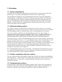
1. Overview
1.1 Scope of application
Network is used to reconstruct phylogenetic networks and trees, infer ancestral types and
potential types, evolutionary branchings and variants, and to estimate datings.
The algorithms are designed for non-recombining bio-molecules. Successful applications
include mtDNA, Y-STR, amino acid, RNA, virus DNA, bacterium DNA, some effectively
non-recombining autosomal DNA, and non-biomolecule data such as linguistic data. By
contrast, recombining bio-molecules will deliver high-dimensional networks which will be
difficult to interpret. Work flow including data preparation and interpretation of results is
described in detail in the next chapters.
1.2 Network building options
The Network software was developed to reconstruct all possible shortest least complex
phylogenetic trees (all maximum parsimony or MP trees) from a given data set. Two different
network-building options are included which can be used independently of each other.
The reduced median or RM network algorithm RM requires binary data (example: at
nucleotide position 16092 each taxon must have either T or C). To allow interpretation of
complex data, a reduction parameter is available. If the reduction threshold r is set to a
sufficiently high number, RM will yield a full median network containing all MP trees.
The median-joining or MJ network algorithm allows multi-state data (example: at nucleotide
position 16092 there can be A, C, G, T, and ambiguities such as N). For larger data sizes, the
parameter epsilon can be set low to calculate sparse networks quickly, or incrementally
increased to calculate higher-resolution networks at the cost of longer run times and increased
network complexity. If epsilon is set to a sufficiently high number, MJ will yield a full
median network (software and memory limits permitting). Optionally, MJ allows external
rooting of the network using an outgroup.
We recommend MJ for general use as first choice. If verification of the MJ results is an issue,
we recommend that RM is then also run on suitably prepared data (nucleotide FASTA data
are easily prepared with the DNA Alignment software).
1.3 Further complexity reduction options
The star contraction option can simplify complex data. The MP option deletes non-MP links
from the network, i.e. links which are not used by the shortest trees in the network. For STR
data or RFLP data, or binary data, a combined RM-MJ calculation may be performed to
simplify the network.
1.4 Complementary options
Network includes a data editor and a graphics program. FASTA files can be imported and
prepared for Network using Fluxus' DNA Alignment software. Higher-quality graphics of
Network's results files can be prepared using Fluxus' Network Publisher software.
5
2. Work Flow
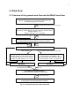
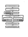
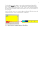
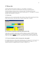
2.1 Overview of the general work flow and the RM-MJ work flow
Prepare your variable data / DNA Alignment
Network will ignore loci (e.g. nucleotide positions) which are
invariable throughout your data set.
rdf
or other format (ami, ych, tor, nex, phy)
Calculate Network
For rooting, use MJ method. If you are a new user, use MJ method.
Weights: default ( = 10)
epsilon = 0 (for MJ) or r = 2 (for RM)
out
MP Option *
Purge superfluous links and median vectors from network.
* kill MP, if too long run time
sto
out
Draw Network
clean, tree-like
high-dimensional cubes or large cyles
Re-Calculate Network :
Change epsilon to 10, 20, 30 etc. (for MJ)
to explore whether and how the network
changes. (For RM change r to 3, 4, 5 etc.)
Re-Calculate Network :
Change weights (see detailed notes).
If this also leads to poor networks, use only
those taxa which contain >1 individuals
MP Option *
MP Option *
when exploring finished
sto
or out
Draw Network / Network Publisher
To lay out final network graphics in high quality
wmf
or emf or bmp or pdf
Import emf picture into MS Powerpoint
or wmf picture into publication/layout software.
Fig. 1a: General overview of the work flow
6
Prepare your binary variable data / DNA Alignment
Network will ignore loci (e.g. nucleotide positions) which are
invariable throughout your data set.
rdf
(binary rdf only), ych, tor
Calculate RM-MJ Network
Run RM (switch off out file generation), then run MJ on the rmf file.
Weights: default ( = 10)
r = 2, no out-file (for RM) and epsilon = 0 (for MJ)
out
MP Option *
Purge superfluous links and median vectors from network.
* kill MP, if too long run time
sto
out
Draw Network
clean, tree-like
high-dimensional cubes or large cyles
Re-Calculate RM-MJ Network :
Change epsilon to 10, 20, 30 etc. (for MJ)
to explore whether and how the network
changes.
Re-Calculate RM-MJ Network :
Change weights (see detailed notes).
If this also leads to poor networks, use only
those taxa which contain >1 individuals
MP Option *
MP Option *
when exploring finished
sto
or out
Draw Network / Network Publisher
To lay out final network graphics in high quality
wmf
or emf or bmp or pdf
Import emf picture into MS Powerpoint
or wmf picture into publication/layout software.
Fig. 1b: Specific work flow for the RM-MJ network calculation
7
2.1.1 Variable data
Network will use only the variable data from your data file or manually entered data set.
Network will ignore invariable data if your file or your manually entered data contains such
data. What do we mean by variable data?
Definition of variable data:
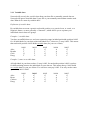
By variable data we mean a genetic nucleotide position, or a genetic locus, or a trait, or a
linguistic feature, or more generally a "character", which allows you to separate your
individuals into at least two groups.
Example 1, variable data:
You have an mtDNA data set, and your sequencing range included nucleotide position 16092
for all individuals. In your data, some individuals are C, others are T at np 16092. This means
that nucleotide position 16092 holds variable data (for your set of data).
Alice
Brenda
Chris
Doug
16091
T
T
G
T
16092
C
T
T
C
16093
G
C
G
G
16094
A
A
T
T
16095
G
C
G
C
Example 2, some in-variable data:
All individuals in your data set have C at np 16092. So nucleotide position 16092 is useless
for differentiating between the individuals in your data set. This means that np 16092 holds
in-variable data for your set of data. You can leave away np 16092. You only need to enter
nps 16091, 16093-16095.
Alice
Bruce
Clarissa
Doug
16091
T
T
G
T
16092
C
C
C
C
16093
G
C
G
G
16094
A
A
T
T
16095
G
C
G
C
8
2.1.2 Preparation of variable data sets for Network
You can enter small data sets using Network's data editor (Start Network / Data Entry menu /
Manual / then select the data type you wish to enter).
Example 3: Network's data editor
Consider the data set in Example 2. You can enter these data in 4 different ways:
1. with the option "DNA nucleotide data", and nps 16091-16095
2. with the option "DNA nucleotide data", and nps 16091, 16093-16095
3. with the option "Binary data", and nps 16091-16095
4. with the option "Binary data", and nps 16091, 16093-16095
For cases 1. and 3., the network-building algorithm will ignore np16092.
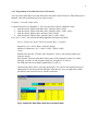
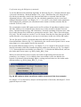
Case 2. Choose the option "DNA nucleotide data" / Continue.
Sequences: 4 (i.e. Alice, Bruce, Clarissa, Doug)
Number of characters: 4 (i.e. 16091, 16093, 16094, 16095)
Create.
Double-click into the "Charact" and "Sequence" cells to enter the np-names and
sequence names.
Note that the Network data editor limits entry of the Character names to 8 (older
Network versions: 6) and Sequence names to a length of 15 (old: 6).
For STR data: the Locus name length limit is 6 (old: 5).
Click into the table cells to enter the nucleotides: You can use the keyboard keys for
editing and for moving up/down/left/right. Alternatively, you can right-click a table
cell and use the context menu to edit the nucleotide.
Fig. 2: Network's Data Editor with dna nucleotide data
9
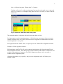
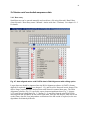
Case 4: Choose the option "Binary data" / Continue.
Continue as for case 2 on the previous page, but enter the nucleotide states compared
to the first sequence. For example, Doug does not have G at 16095, so enter 0 into his
16095 cell.
Fig. 3: Network's Data Editor with binary data
The maximal number of characters allowed in the data editor is 1000.
For long sequences with sequencing ranges > 1000 it becomes necessary to leave away nonvariable characters (here: np 16092). But note that for large data sets manual data entry and
manual alignment is error-prone.
For larger data sets in FASTA files, we request you to use Fluxus' DNA Alignment software.
Example 4: DNA Alignment software
DNA and amino acid FASTA files can be imported and prepared for Network using Fluxus'
DNA Alignment software. This software has a limit of 99999 on the number of characters and
no limit on the number of sequences. The DNA Alignment software can be run with or
without the auto-alignment option.
Alignment algorithms vary in quality, and poor auto-alignment results will lead to poor
network results.
10
The alignment algorithm in Fluxus' commercial DNA Alignment software is a sophisticated
pairwise alignment algorithm which compares whole segments of sequences and does not
employ gap penalties. If the user chooses to run this algorithm, all sequences in the FASTA
file will be auto-aligned under a reference sequence which the user can choose. Normally the
user will choose an arbitrary sequence from the data set as a reference sequence; for the
special case of human mtDNA, the choice can be the Cambridge Reference Sequence, but
nucleotide numbering must be consistent between the data set and the CRS.
Alternatively, the DNA Alignment software can import FASTA files and export them as
Network-rdf format without alignment. This option can be useful if your FASTA data are prealigned by other programs, or if your data set fits into the Network-limit of 1000 characters
without alignment.
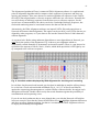
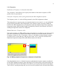
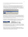
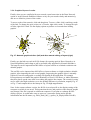
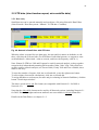
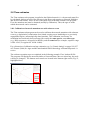
As a general rule: Before using unknown aligned data or auto-aligned data in Network, you
must check the quality of the alignments. Fig. 4 shows a poor alignment which we
intentionally created manually to demonstrate an insertion artefact: There is a gap inserted at
np16096 in the sequences Nuu1b, Nuu1c, Nuu2a, which shifts nps16096-16109 right by one
np compared to the reference sequence.
Fig. 4: Insertion artefact displayed by DNA Alignment for checking and correcting
In real data, check around each inserted gap, but bear in mind that an artefact will not always
be so obvious. Check each nucleotide mismatch (Fig. 4, 16111.T in Nuu5a and Nuu5b)
against the sequencing chromatograms to confirm validity of the nucleotide. Investigate each
ambiguous nucleotide. Double-check newly discovered mutations against the possibility of
contaminations and sequencing errors.
If you do not check unknown data or auto-aligned data, you risk that Network will build an
incorrect network. Note that the Network Data Editor does not highlight alignment differences
and does not allow alignment editing, but that we recommend the DNA Alignment software
to display and manually edit alignments.
11
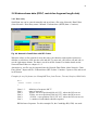
2.1.3 Weights
Introduction: Genetic Distances and Weights
A fundamental concept within network-building algorithms is the genetic "distance" between
two sequences in a data set. This is calculated by the number of different characters between
these sequences. To explain the genetic distance, let us look at two sequences:
16091
16092
16093
16094
16095
Alice
T
C
G
A
G
Bruce
T
C
C
A
C
Bruce differs from Alice in two characters, 16093 and 16095. The genetic distance is 2.
To take into account that some characters can be more important than others, Network applies
a weight to each character. Consider the example with Network's default weight of 10:
16091
16092
16093
16094
16095
Alice
T
C
G
A
G
Bruce
T
C
C
A
C
Weight
10
10
10
10
10
Bruce differs from Alice in two characters, 16093 and 16095. The weighted distance is 20.
Let us assume that there are 100 more sequences in the data set and that character 16095 is
hypervariable within the data set. A frequently changing character is less valuable for network
construction than infrequently changing characters. Therefore we downweight 16095:
16091
16092
16093
16094
16095
Alice
T
C
G
A
G
Bruce
T
C
C
A
C
Weight
10
10
10
10
5
Bruce differs from Alice in two characters, 16093 and 16095. The weighted distance is 15.
For first network-building calculations with a new data set, we suggest that you leave the
default weights. If your network turns out to be poor (containing high-dimensional cubes or
large cyles), you can change the weights for the next runs as explained on the following
pages.
Types of weight in Network:
In Network, you can change two types of weights:
1. weights of characters. This value may range between 0 and 99. A value of 0 instructs
Network to ignore the character. 10 is the default value.
2. in MJ only: weights of single nucleotide mutation types (transversions, transitions).
This weight may range from 1:50 to 50:1. The default is 1:1.
12
Guidelines for changing weights, if the calculation with defaults is unsatisfactory:
1. Increase the weight for events that might be much less likely to happen, because they are
significant when they do happen.
2. Decrease the weight for events that might be much more likely to happen.
3. For characters in which deletions or insertions have occurred, we suggest a double weight
(weight value 20)
4. For human mtDNA data, we suggest transversions to be weighted three times as high as
transitions. (Transversions occur about 20x less often than transitions in human mtDNA,
see Fig. 8)
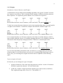
5. For hypervariable sites/characters (including length/repeat mutations in mixed data), we
suggest downweighting the character to 5 or even 0. To identify a hypervariable or fastmutating character within your network, draw the network and press the statistics button
(see fig. 5, character 176)
Fig. 5: Statistics-button to identify fast-mutating character for downweighting
Before you change weights, decide whether you want to save the changed weights or not.
Note: For all data, including STR data and "mixed" data, you can save changed weights
(from Network 4.5.0.0 upwards).
13
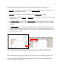
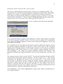
To change weights without saving, go into the Network Calculations main menu, into either
the Reduced Median (RM) option or the Median Joining (MJ) option. Then open the rdf file,
open the Parameters menu, Change weights (see Fig.6). Click onto the line for which you
want to edit the weight, and a "New Weight" entry field will appear with the current weight.
Edit this weight and click OK.
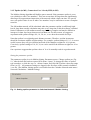
Fig. 6: Editing character weights in Network's Calculation / Parameters
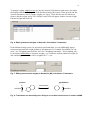
In the Median Joining option, for non-binary nucleotide data, you can additionally apply a
transversions/transitions weight globally to all characters. For example for mtDNA you can
enter 3 for "Weighting transversions" and 1 for "Weighting transitions". This weighting will
be interpreted additionally to character weights, e.g. a character with the character weight 20
and containing transversions will be weighted 20 * 3 = 60.
Fig. 7: Editing transversion weights in Network's (MJ) Calculation / Parameters
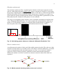
purines
A
pyrimidines
transversion
T
transition
G
transition
C
Fig. 8: Transitions are chemically more likely to occur than transversions in human mtDNA
14
To edit weights and save the changes, to into the Data Entry main menu, Import rdf file,
specify the file type, and click Continue. This will load the file and open Network's Data
editor. To edit a weight, click into the cell (see Fig. 8), type a value, and confirm by hitting
the <Enter> key or clicking into a different cell. Finally, click the Save button to update the
rdf file, and Exit.
Note: For STR data, you can now also edit weights in the Network STR editor and save the
weights in the new ych format. (From Network 4.5.0.0 upwards.)
Fig. 9: Editing character weights in Network's Data Editor
15
2.1.4 Frequency
Definition of "Frequency" in Network's data editor
The "frequency" value allows you to specify the number of times that a sequence or STR
profile occurs in your data set.
Fasta files: Frequency value in files generated by the DNA Alignment software
The frequency value is 1 in the rdf-files generated by the DNA Alignment software.
This means that one sequence entry corresponds uniquely to one taxon (i.e. to one individual)
in the rdf-files generated by DNA Alignment, if the sequence names are unique within the
FASTA file. DNA Alignment can create duplicate taxa with identical names when truncating
long names (longer than the name length 6 permitted by Network), but Network will issue a
warning message when such a file is imported.
Manual data entry: Frequency value
If the same sequence (or STR profile) occurs several times in your data set, you do not need to
enter this several times in Network's Data Editor. Instead, you can click into the cell in the
Frequency column (see Fig. 10) and type a value (i.e. the number of times that the sequence
or profile occurs in your data set), and press the <Enter> key or click into a different cell.
Duplicated sequences (and profiles) with different names are allowed.
Fig. 10: Editing sequence frequencies in Network's Data Editor
Note that duplicate taxa (i.e. identical sequences with identical sequence names) are allowed
by the DNA Alignment software when importing FASTA and saving as rdf. Such rdf files can
be opened by the Network Data Editor, but cannot be processed by the Network Calculation.
There will be a warning message and you can correct the problem in the Network Data Editor.
16
2.1.5 Epsilon (in MJ), Connection Cost / Greedy FHP (in MJ)
The Median Joining algorithm will build a sparse network if the parameter epsilon is set to
zero (default) or other "low numbers". This can cut run-time for large data sets significantly,
allowing a first approximate impression of the network within a short run time. For special
cases, an epsilon value of zero or other "low numbers" may be sufficient to create a complete
network.
The full median network will be calculated when the parameter epsilon is sufficiently high,
but for large data sets this calculation may take a very long time or hit the software’s internal
limits. Furthermore, a full median network may look very complex and may be difficult to
interpret, for data sizes larger than non-trivial data sets. For this reason, we suggest to
experiment with epsilon-settings of 0, 10, 20, etc., to see how the network develops.
Note that epsilon is a weighted genetic distance measure. Therefore, epsilon increments
should be consistent with the weight settings. For example, epsilon settings of 1,2,3,..9 are not
useful, because they will give identical networks if the character weights are 10 or greater.
Conversely, epsilon settings of 10, 20, 30, etc can be useful if the character weights are 10 or
greater.
Our experience suggests that epsilon-values of 0 or 10 normally result in a good network.
Setting the parameter epsilon:
The parameter epsilon is set in Median Joining, Parameters menu / Change epsilon (see Fig.
11), after the data file has been opened (File menu / Open). To change the value of epsilon,
type a number, or click the <up> or <down> button, and click OK. Epsilon values may range
from 0 to 231. All parameter settings are logged in the first lines of the network calculation
*.out file. (The Median Joining option is accessable from the Calculate Network main menu /
Network Calculations / Median Joining.)
Fig. 11: Setting epsilon parameter in Calculate Network / Median Joining
17
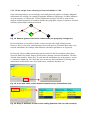
What does epsilon mean?
The parameter epsilon specifies a weighted genetic distance to the known sequences in the
data set, within which potential median vectors may be constructed. If epsilon is set less than
the greatest weighted genetic distance within the data set, then there is a theoretical possibility
that the MJ network will not contain all possible shortest trees. If epsilon is set equal to (or
greater than) the greatest weighted genetic distance, the MJ algorithm is guaranteed to yield a
full median network. Usually we find epsilon=10 to be sufficient.
The range of (unweighted) genetic distances can be calculated and displayed with Network's
Tools / Mismatch Distribution (Fig. 12). In this example, the maximal pairwise difference is
shown as 4. If all character weights are 10 and the transversion/transition weighting is 1:1,
then an epsilon value of 40 will guarantee a full median network for this example.
Fig. 12: Calculating genetic distances in Network's Mismatch Distribution Tool
What is a median vector?
A median network consists of nodes, and links which connect the nodes. The nodes are either
sequences from the data set, or median vectors. The links are character differences. A median
vector is a hypothesised (often ancestral) sequence (see Fig. 13, mv1 and mv2) which is
required to connect existing sequences within the network with maximum parsimony.
Without the median vector, there would be no shortest connection between the data set's
sequences.
ALICE
16094
16095
BRUCE
16093
mv1
mv2
16094
16091
16095
DOUG
Fig. 13: Median network showing median vectors mv1 and mv2
CLARISSA
18
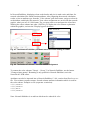
Switching the distance calculation method between Connection Cost and Greedy FHP:
The switch between the two available distance calculation methods (default "Connection cost"
method of Röhl et al, alternative "Greedy FHP" method of Foulds, Hendy, Penny et al) is set
in Median Joining, Parameters menu / Criterion (see Fig. 14), after the data file has been
opened (File menu / Open). To change the distance calculation method, click onto the
"Criterion" line in the Parameters menu. This will change the method and close the menu.
When you re-open the Parameters menu, the currently active method is shown (e.g.
"Criterion: Greedy FHP").
Fig. 14: Distance calculation method. Click "Criterion" line to change from the default
"Connection cost" method (left) to the alternative "Greedy FHP" method of Foulds,
Hendy, Penny (right)
19
2.1.6 Reduction threshold r and out file option (in RM network option)
The Reduced Median algorithm will build a reduced network if the parameter r is set to 2
(default) or other "low numbers greater than two". The reason for "reducing" a full median
network is to improve clarity for data sizes larger than trivial data sets, because a full median
network can easily contain too many links and median vectors to visualise and interpret.
The full median network will be calculated when the parameter r is sufficiently high, but this
network may be difficult to interpret. For this reason, we suggest to experiment with r-settings
of 2, 3, 4, 5, etc., to see how the network complexity increases.
Note that r is a weighted genetic distance ratio for the likelihood of parallel mutations (see
Fig. 16).
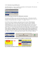
Setting the parameter r:
The parameter r is set in Reduced Median, Parameters menu / Changing reduction threshold
(see Fig. 15), after the data file has been opened (File menu / Open). To change the value of r,
type a number and click OK. All parameter settings are logged in the first lines of the network
calculation *.out file.
(The Reduced Median option is accessable from the Calculate Network main menu / Network
Calculations / Reduced Median.)
The reduction threshold value is a real number which should be set to at least 2. For human
mtDNA control region sequences, the value 2 works ok. Sensible values for other data need to
be determined experimentally by increasing r and seeing whether shorter MP trees are then
generated. Generally, the longer the branches in the data set, the higher the r setting should be.
Fig. 15: Setting Reduction threshold parameter in Calculate Network / Reduced Median
20
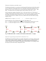
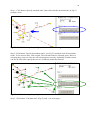
What does the Reduction threshold r mean?
The Reduction threshold r is a parameter for deleting parallel mutations in ladder-like meshes
(Fig 16, right) from a full median network. The reasoning is that parallel mutations (Fig. 16,
character 19101) are more likely to have occurred between existing sequences (Kay – John,
Mary – Nat) than between an existing sequence and a median vector (Lucy – mv1).
In this example the weights of characters 19101, 19102, and 19103 are 10. If the sum of
weights on the long side of the ladder (characters 19102 and 19103) is greater or equal r times
the weight of the parallel mutation (character 19101), the reduction algorithm deletes the
parallel mutation between a median vector (mv1) and the other side of the ladder (existing
sequence Lucy):
sum (character weights long side of ladder)
>=
r * character weight parallel mutation
In this example the sum of weights on the long side of the ladder is 20.
For r = 2, r times the weight of 19101 is 20, so mv1 and the links are deleted (Fig 16, left).
For r = 3, r times the weight of 19101 is 30, so mv1 is not deleted (Fig 16, right).
JOHN
NAT
mv1
JOHN
19102
19101
19101
19102
KAY
19101
LUCY
19101
19102
19103
MARY
NAT
19103
KAY
19101
19103
LUCY
MARY
Fig. 16: RM network with r = 2 (left) and full median network with r = 3 (right)
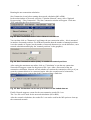
Option for not generating an out file (New in Network 4.5.1.6)
The RM network calculation produces an rmf file with split loci in a first step, and an out file
with a network in the second step. Optionally the second step can be switched off (checkbox
"Generate list of links (out file for drawing)". The rmf file can then be used for the MJ
network calculation. This combines the advantages of both methods: Locus splitting of RM,
and improved speed and memory management of MJ.
21
2.1.7 MP option to clean up networks
A full median network (parameter epsilon in MJ-calculation or parameter r in RMcalculation set sufficiently high) contains all possible shortest (MP or Steiner) trees.
However, the network calculations can also produce unnecessary median vectors and
links (see fig 18, mv5, mv8-mv18). The MP option (Polzin et al, see fig 19) identifies
the unnecessary median vectors and links, which can be switched off in the results
display (see fig 20).
OR3
OR1
mv19
mv3 AX OR2
mv6
O3
mv4
mv2
BA
B1
mv7
CH5
A11 CH12
A12
mv1
CH4
GO1
MAC
BAB1
BAB2
CISAB
GO3
Fig. 17: ExampleAminoAcids.ami, MJ with epsilon=10, cleaned up with MP
OR3
mv20
OR1
mv12
mv15
mv19
mv11
AX
mv3
OR2 mv7
MAC
O3
mv13
mv4
mv6
CH5
BAB1
A11
CH12
mv2 mv5 mv14
BA mv1 A12
mv16 CH4
GO1CISAB
B1
mv17
mv8
mv18
GO3
mv9
mv10
BAB2
Fig. 18: ExampleAminoAcids.ami, MJ with epsilon=10
Note: After MJ-calculation of ExampleAminoAcids.ami with epsilon=0, the network looks
identical to fig 17, except that the blue links and mv3 are missing, meaning that trees are
missing. MJ with epsilon=10 finds all trees (fig 18), and MP cleans up the network (fig 17).
22
Running the MP calculation
We recommend that the MP calculation is generally run on all *.out files produced by the MJ
or RM network calculations. In the main window of Network, select the "Calculate Network"
menu, select "Optional Postprocessing" / "MP Calculation". The MP calculation options
window will appear. Leave the default radio-button active ("Network containing all shortest
trees, and list of some shortest trees sufficient to generate this network"). Click the "Start"
button to select the *.out file and run the MP calculation. The MP calculation results are saved
into the same folder, into a file with the extension *.sto.
Fig. 19: MP Calculation (Polzin et al) is recommended after every network calculation
Displaying the results
Select the Network Draw subprogram, or start the Network Publisher software. File menu,
Open, select the *.sto-file. At the pop-up window, click the "No" button, if you are interested
to compare the original network with the cleaned-up network. When the network graphic is
completed, you can compare the cleaned up network with the original network by switching
between the radio buttons "Network" and "Original Network".
Fig. 20: Draw subprogram
After activating the radio button "Tree(s)", you can interactively display a list of shortest
trees. This list does not contain all shortest trees in the network. The list only contains all
shortest trees which are sufficient to define all the network nodes and links (see chapter 2.2.3
for a graphic example).
23
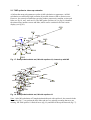
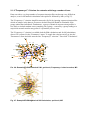
2.1.8 Star Contraction option: Use for network simplification, or for
identification of population expansion events
Complex networks containing many sequences, taxa or Y-profiles can be very difficult to
interpret at first glance. One option to reduce complexity is the star contraction algorithm,
another option is described in sub chapter 2.1.9.
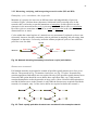
Historic demographic expansion events are characterised by star-like clusters of nodes around
a founder population node. The star contraction algorithm identifies such clusters and shrinks
the nodes of a cluster back towards the founder node. The star contraction algorithm therefore
has two separate uses:
a) to help analyse networks for historic demographic expansion events, and
b) to help simplify complex networks into "skeleton" networks for a first overview.
NUU7
NUU5A
NUU8A
NUU9A
NUU10
NUU6A
NUU12A
NUU11A
NUU14
mv6
NUU17
NUU13
NUU15A
NUU18A
mv5
NUU16
NUU20A
NUU21A
mv2
NUU4
NUU28
NUU19
mv3
NUU27
mv4
mv9
mv8
NUU3
NUU23
mv7
NUU22A
NUU1A
mv1
NUU24A
NUU2A
NUU25A
NUU26
Fig. 21: ExampleDNAMultistate.rdf : Star-like cluster around founder node NUU11A
NUU11A
NUU7
NUU17
NUU6A
mv5
NUU18A
mv
4
NUU16
NUU4
NUU28
NUU21A
NUU27
NUU20A
NUU19
NUU23
NUU3
NUU1A
NUU22A
sco1
NUU24A
NUU2A
Fig. 22: Same data with star-contraction preprocessing (mv1 renamed to sco1)
24
Running the star contraction calculation
Star Contraction is run before running the network calculation (MJ or RM).
In the main window of Network, select the "Calculate Network" menu, select "Optional
Preprocessing" / "Star Contraction". The Star Contraction window will appear. Click onto
"File" and select the file to be processed.
Fig. 23: Star Contraction is used before Network calculations
You can then click on "Parameters" and change the star contraction radius – this is measured
in number of mutated positions. For STR/microsatellite data the number of mutated positions
is not the number of repeats, but the number of network characters (to see the difference, run a
network calculation and display the "mutated positions" in the graphics).
Fig. 24: Star Contraction radius (delta), in number of mutated positions
After setting the maximum star radius, click on "Calculation" to run the star contraction.
Network will suggest a name for the protocol file *.pro. After a first round of the star
contraction calculation, Network will ask whether to continue the contraction; click yes if you
want the contracted data to be contracted again. After the second round of contraction,
Network allows you to contract the doubly contracted data a final time.
Fig. 25: Star Contraction can be run up to 3 times on the loaded data set
Finally Network suggests a name for the star contraction results file *.sco.
The *.sco file can be used for the network calculation (MJ or RM).
After the network calculation, the results file *.out can be used for the MP option to clean up
the contracted network.
25
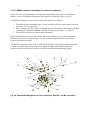
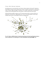
2.1.9 "Frequency>1" Criterion for networks with large number of taxa
Data sets with a very large number of sequences/taxa/profiles can become very difficult to
analyse, even for MJ network calculation with epsilon=0 followed by MP (see fig 27).
The "Frequency>1" criterion simplifies networks (fig 26) by ignoring sequences/taxa/profiles
which are unique in the data set, because a skeleton network should be obtainable from
groups rather than individuals. Furthermore, a group of identical sequences/taxa/profiles is
less likely to include random errors (sampling, lab, typing) – conversely a group leading to a
suspicious network artefact may point to a systematic process error.
The "Frequency>1" criterion is available both for RM calculations and for MJ calculations,
after a file is opened, in the "Parameters" menu. To toggle the criterion on/off, go into the
"Parameters" menu and click onto the line "Frequency>1 criterion". Then click "Calculation".
MA76
NI3
NI4
KRY39
KRY35
TIB152
18P110
SA114
ITL60
KRY37
NI8
2P102
25P94 VNTW51
VN37
1P89
KN105
mv7
M_P114
MA75
SES54
TIB153
KN96 CHU46
KRY42
2P115
UD21
mv9
MCTW28
mv1
MA82
CHU55
UD25
TW56
EVUD27
UD24 MULT62 21P43
SES53
EV28
mv2
mv3
CHU56
EVUD30
EV31
SA111 MA74
TW65
MC20 M_P27
TIB140
18P129
EV32
mv8
EV29
MULT54
MULT25 KRY44 KRY65
mv4
MULT55
SA115 mv6
EV33
NI12
MMSA83
NI10
TIB131
TW57
mv5
CHU49
UD23
SA106
2P46
SA109
18P69
2P112
1P107
MAVN33
TIB143
SA112
CHU50
CHU40
Fig. 26: ExampleRFLPWeighted.rdf: MJ, epsilon=0, Frequency>1 criterion active, MP
Fig. 27: ExampleRFLPWeighted.rdf: MJ calculation, epsilon=0, MP
26
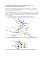
2.1.10 RM-MJ network calculation for reduced complexity
Data sets with a very large number of sequences/taxa/profiles can become very difficult to
analyse, even for MJ network calculation with epsilon=0 followed by MP (see fig 27).
The RM-MJ technique is used to reduce network complexity as follows:
1. The RM network calculation stage 1 (result: rmf file) splits loci on the basis of how far
apart they are in the network.
2. After saving the rmf file, stage 2 of the RM network calculation is not required (in RM
/ parameters / reduction threshold: uncheck "Generate list of links" – see Fig 15).
3. The rmf file is used for the MJ network calculation.
Result: the RM-MJ network is often simpler than a pure MJ network, because implausible
parallelisms have been avoided in step 1 (see fig. 28 where additionally star contraction
preprocessing has been used).
The RM-MJ technique can be used for STR data, RFLP data, binary data, and binarised dna
or amino acid data. (When binarising dna or amino acid data with the DNA Alignment
software, please read the notes on binary rdf files in the DNA Alignment help pages.)
TW59
2P91
KN100
TW60
MAVN33
VN36
1P103
KN99
1P99
2P90
2P102
TW61
SCO1
MULT55
MA71
21P106
1P107
KN105
MULT54
SCO5
SCO9
MC20
TW56
SA112
VN34
MM88
MC19
MA76
SA122
MMSA83
2P46
KRY37
SA106
SCO3
MA73
CHU49
1P152
MA78
TIB135
VN31
VN38
KN102
MA81
CHU40
Fig. 28: ExampleRFLPWeighted.rdf: Star contraction, RM, MJ, and MP calculation.
27
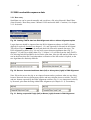
2.2 DNA nucleotide sequence data
2.2.1 Data entry
Small data sets can be entered manually and saved into a file using Network's Data Editor
(Start Network / Data Entry menu / Manual / DNA nucleotide data / Continue). See chapter
2.1.2 for details.
Fig. 29: Loading FASTA data into DNA Alignment with or without alignment option
Larger data sets should be imported into the DNA Alignment software in FASTA format,
aligned (if required), checked (see chapter 2.1.2), and exported for Network in rdf-format.
This allows longer sequences to be analysed than with Network's manual data entry. The
DNA Alignment software (Fig. 30) can easily export character/multistate data (Fig. 2 /
chapter 2.1.2) rdf files or binary data (Fig. 3 / chapter 2.1.2) rdf files from the same FASTA
file, allowing both MJ and RM to be run on the same data. After the MJ analysis, RM can be
run on the binary data file if an independent verification of the MJ results is required, as the
two algorithms are distinctly different.
Fig. 30: Save as character/multistate data (left) or binary data (right) in DNA Alignment
Note: Please do not use the phy or nex import formats unless you know what you are doing,
because Network does not perform any checks and may calculate incorrect results. The phy
and nex formats exported by the DNA Alignment software (Fig. 31) are interpreted correctly
by Network; prior data checking within DNA Alignment (see chapter 2.1.2) is mandatory.
Fig. 31: Saving sequential Phylip (left) or Nexus (right) formats in DNA Alignment
28
2.2.2 Network calculation using the MJ algorithm with optional external rooting
Calculating the initial network
In Network (Fig. 32): Calculate Network menu / Network Calculations / Median Joining.
File / Open / DNA data file (rdf). Select the rdf file which you manually created in the
Network Data editor or exported from the DNA Alignment software. After opening the file,
the calculation parameters can be viewed and changed (Parameters menu), see chapters 2.1.3
– 2.1.5 for details on the parameters. After changing the parameters, the calculation can be
started (Calculate network) and the result file is saved (*.out).
Fig. 32: Opening the rdf data file for MJ network calculation
We recommend to run the MP option on the out-file to delete all superfluous median vectors
and links which are not contained in the shortest trees in the network (Calculate Network
menu / Optional Postprocessing / MP Calculation / Network containing all shortest trees, and
list of some shortest trees sufficient to generate this network / Start / Open Network output
file [out]). The MP results are saved as *.sto file format.
The sto-file can be opened, viewed and analysed in the Draw Network option (See Fig 32,
first menu line), or in the Network Publisher software (Fig. 33). Alternatively, the out-file can
be opened. Save a screen snap (bmp) or a vector graphic (emf/wmf) of the network.
Fig. 33: Opening the sto-file or the out-file for visual display and analysis
Re-run with different settings (see Fig. 1 in chapter 2.1). For example if the network is messy,
identify nucleotides which have mutated frequently within your data set (see Fig. 5 in chapter
2.1.3), downweight these nucleotides (see chapter 2.1.3), calculate the MJ-network, and save
the results under a new name (e.g. DNA_multi_MJ_2.out).
When your network looks clean, keep the successful weight settings and increase the
parameter epsilon (see chapter 2.1.5) to identify where new median vectors are added to the
network. Experiment with increasingly higher epsilon settings and each time save the results
under different names (e.g. DNA_multi_MJ_2_epsilon_20.out).
29
Rooting the network, ancestral node, root proxy node
The process of determining the ancestral node is referred to as "rooting the network". The
ancestral node of a network can be determined by comparing the network nodes with suitable
outgroups. For example, to (manually) find the ancestral node of a network of domestic
horses Jansen et al used zebra and wild asses as outgroups (Jansen T, Forster P, Levine MA,
Oelke H, Hurles M, Renfrew C, Weber J, Olek K. Mitochondrial DNA and the origins of the
domestic horse. Proc Natl Acad Sci USA. 2002 Aug 6;99(16):10905-10.).
We recommend the new “External rooting: active” parameter in the MJ network calculation.
First, you need to add your outgroup to the intraspecies *.rdf file. This procedure is facilitated
by the DNA Alignment software version 1.3.2.0 (for release in January 2011) which allows
you to merge an outgroup-alignment (*.ali file) into an intra-species alignment (*.ali file) and
export this as an *.rdf file.
We recommend users to first align the intra-species sequences without the outgroup, because
the automatic alignment algorithm is designed for closely related sequences. We recommend
aligning just the outgroup sequence to the reference sequence in a new session, to minimise
manual editing work. Finally, merge the *.ali files using the “Import alignment” function in
DNA Alignment 1.3.2.0, which can introduce additional insertions and deletions. After
manually checking that no alignment problems occurred in this merging step, export the *.rdf
file.
The outgroup sequence must be named “ROOT”. The network calculation will ignore ROOT
during network construction with the parameter “External rooting: active”. After network
construction, the algorithm will search for the root proxy node, i.e. the nearest existing
network node to the ROOT sequence, taking the specified character weights into account.
Note that the actual network root may lie within an adjacent (multi-mutation) link and some
mutation re-ordering along this link and the generation of a new median vector may be
required. Generation of a new "root" median vector and re-ordering of mutations has not been
implemented due to significant computational complexities.
Network Publisher 1.3.0.0 is able to highlight the root proxy node, which is a useful feature in
very complex networks.
30
2.2.3 Discussing, analysing, and interpreting network results (MJ and RM)
Homoplasy, cycle, reticulation, cube, hypercube
Mutation of a genetic site can occur at different times and independently of previous
evolution. Figure 34 below shows characters 16094 and 16095 occurring twice in the
network; this is referred to as parallel mutations or homoplasy. In this special case, the
characters in the network form a cycle (cycles may have more than 4 sides) or reticulation.
Box-like cycles are sometimes referred to as a cube (or hypercube in the case of a 4dimensional box or more).
Cycles within the central regions of a network are not uncommon. Peripheral cycles are not
necessarily incorrect, but they sometimes point at problems in sampling, lab processing, data
alignment, or data entry. Conversely, networks without peripheral cycles are not sufficient
proof for error-free data.
ALICE
16095
BRUCE
16093
16094
mv2
mv1
16094
16091
CLARISSA
16095
DOUG
Fig. 34: Network showing homoplasy in the form a cycle (reticulation)
Shortest trees in network
Full median networks are designed to contain all possible equally shortest trees for a given
data set. The network in Fig. 34 contains 4 such trees, see Fig. 35 below. Networks may
contain superfluous links which are not required for any of the possible equally shortest trees.
Network's MP option should be run to delete these superflous links, esp. if the network
contains homoplasies such as hypercubes or large cycles. (Note: Network's MP option does
not find all shortest trees in the network, it only finds the shortest trees required to build the
network; for example, only 2 of the 4 trees below are required to define the network.)
Fig. 35: The 4 equally probable shortest trees contained in the example network
31
Groups, clades, haplotypes, haplogroup
In phylogenetics, the network nodes are living or extinct sequences with specific mutations.
Descendants of a node can be grouped into a cluster or branch, also known as a clade (greek
klados, branch). When the number of characters (loci) under consideration is extended, the
sequence may be differentiated into sub-sequences, and the branches become longer.
Individual human mtDNA sequences and Y chromosomal profiles are often referred to as
haplotypes in the literature, although these two loci are necessarily haploid. In this usage,
branches and clusters are sometimes referred to as haplogroups.
TW59
2P91
KN100
TW60
MAVN33
VN36
1P103
KN99
1P99
2P90
2P102
MULT55
TW61
SCO1
MA71
21P106
1P107
KN105
MULT54
SCO5
SCO9
MC20
TW56
SA112
VN34
MM88
MC19
MA76
SA122
MMSA83
2P46
KRY37
SA106
SCO3
MA73
CHU49
1P152
MA78
TIB135
VN31
VN38
KN102
MA81
CHU40
Fig. 36: Human mtDNA network showing branching and clustering. Displayed names
are for sequences, not haplotypes. See file ExampleRFLPweightedRMMJ.out.
32
2.2.4 Graphical layout of results
Finally, when you are satisfied with your network, spend some time in the Draw Network
option or in the Network Publisher software to lay out your results clearly and attractively,
and save a definitive picture of the results.
To move nodes of the network, click and drag them. To move a link, click it and drag a node
of the link. To change the style (colour etc.) of nodes, right-click a node. To change the style
of links, right-click a link. Use the display options to produce a clear and clean-looking
graphic.
Fig. 37: Network graphics before (left) and after manual editing of layout (right)
Finally, save the laid-out work in fdi file format (for opening again in Draw Network or in
Network Publisher) and in bmp or pdf or emf/wmf (only supported in Network Publisher).
The bmp file can be imported into MS Office or layout software as a limited-resolution noneditable graphic.
The emf file can be imported into MS Office or layout software as a high resolution, editable
graphic. After importing the emf or wmf graphic, ungrouping the graphic object is normally
required. Font sizes and graphic re-scaling will depend on the application. For example
Powerpoint may not handle the graphic identically to Word, Corel Draw, or Adobe Illustrator,
therefore plan to spend some time on tweaking the graphic after import. The reward for using
emf or wmf is the high resolution: to see the striking difference in resolution, magnify Fig. 36
or Fig. 37 and compare this to the bitmap in Fig. 5 at high magnification.
Note: In the current software version, the fdi file is saved specific to the display setting of the
computer on which it was saved. This means that the size and position of the network graphic
may change if the file is opened on a different computer. If you plan to exchange fdi files
during a project, it would make sense to agree on a consensus setting and to put this
information into the file name (e.g. DNA_multi_MJ_2_epsilon_20_display1400x1200.fdi).
33
2.2.4.1 Node and pie chart colouring in Network Publisher 1.3.0.0
Node colouring and pies are increasingly used within network graphics to display additional
information in a network, for example geographic affiliation, haplogroup, or ethnic affiliation
of each sequence or STR-profile. Colour-coded nodes and pies can also be used to help
analysis and interpretation, for example whether the geographic origins of sequences correlate
with their relationships within the network.
Fig. 38: Network graphic with colour-coded nodes (for geography, lineage etc.)
In Network Draw it is possible to define colours and pies after right-clicking a node.
However, this is a lot work, and furthermore this work must be performed again after every
network calculation (for example when different calculation parameters are explored).
In Network, colour-coding information may be entered in the Network data editor (Start
Network, Data Entry menu, Import rdf file) before running a network calculation: Click the
"Switch input window" button (fig. 39) and enter the information for each sequence in max
15 characters length (fig. 40). Note that you can also use these attributes for storing other
information such as home town, food preferences, metabolic disorders, etc.
Fig. 39: In the data editor, switch between sequence entry and attribute entry
Fig. 40: Entry of attributes for later colour-coding (Network 4.5.0.0 or later versions)
34
In Network Publisher, displaying colour-coded nodes and pies is made easier and faster for
network calculation files which contain attributes: After importing the network calculation
results, select an attribute type from the "Color scheme" pull-down menu, assign a colour for
each attribute, and display the network. Your colour assignments are saved with the network
graphic, when you save in *.fdi format (Tip: you may want to cut and paste the 6 last lines
defining the colour scheme into other *.fdi files). To display the color scheme explanation
within the graphics, activate the "Display legend" checkbox.
Fig. 41: The Network Publisher pull-down menu for colour-coding of nodes
Fig. 42: The Network Publisher menu for colour assignment
To rename the color schemes "Group1 – Group 3" in Network Publisher, use the button
"Change scheme names". Renaming is only possible in Network Publisher, not in the
Network rdf / STR editor.
Attributes can also be imported into a Network Publisher 1.3.0.0. session from Excel or a csvfile. First column: sequence names. Second column: attribute information which is used for
the color scheme. Example csv file (separator: semicolon):
S001;FEMALE
S002;FEMALE
S003;MALE
S004;FEMALE
Note: Network Publisher is an add-on which can be ordered for a fee.
35
2.2.5 Verification using the RM option
The RM algorithm is a separate and different algorithm to the MJ algorithm. This makes the
RM option suitable for verifying MJ networks.
Fig. 43: Opening the rdf data file for RM network calculation
In contrast to MJ, RM can only work with binary data (see Fig. 3). If the data set for MJ
consists of binary data, the same file can be used for RM. Otherwise the data set needs to be
binarised. For manual data entry, see chapter 2.1.2, example 3, case 4.
For FASTA file data, binarisation is automatically carried out by the DNA Alignment
software when saving as "Network binary data format" (see Fig. 29, right). The DNA
Aligment software will write "N" into some positions, when the character is multistate.
Network RM will give a warning message and automatically replace these Ns in a "greedy"
manner minimizing the distance to all other sequences within the dataset, when the file is
opened (Fig. 43). You can also import this binary rdf file (Data Entry / Import rdf file / Binary
Data / Continue / select the file and open) into the Network Data Editor. A warning message
appears and Ns are highlighted red. To see how Network replaces each N with either 0 or 1
use the "Replace" and "Undo" buttons (Fig. 44). If there are more than 5 characters with N,
we suggest to delete these characters in the Network Data Editor by right-clicking the cell in
the "character" header row and choosing "delete character" (Fig. 45); then save and exit.
Fig. 44: Binary rdf files containing "N", and button to replace the Ns
Fig. 45: Delete characters containing "N" in the Network Data Editor
36
Verification using the RM option (continued)
To run the RM network calculation algorithm: In Network (Fig. 43): Calculate Network menu
/ Network Calculations / Reduced Median / File / Open / DNA data file (rdf). Select the rdf
file which you manually created in the Network Data editor or exported from the DNA
Alignment software. After opening the file, the calculation parameters can be viewed and
changed (Parameters menu), see chapters 2.1.3, 2.1.4, and 2.1.6 for details on the parameters.
After changing the parameters, the calculation can be started (Calculate network) and the
result file is saved (*.out).
We recommend to run the MP option on the out-file to delete all superfluous median vectors
and links which are not contained in the shortest trees in the network (Calculate Network
menu / Optional Postprocessing / MP Calculation / Network containing all shortest trees, and
list of some shortest trees sufficient to generate this network / Start / Open Network output
file [out]). The MP results are saved as *.sto file format. Note that for some data sets the MP
option may take a very long time to run (up to several days); in this case, kill the MP option.
The sto-file can be opened, viewed and analysed in the Draw Network option, or in the
Network Publisher software (Fig. 33). Alternatively, the out-file can be opened. Save a screen
snap (bmp) or a vector graphic (wmf) of the network.
Re-run with different settings (see Fig. 1 in chapter 2.1). For example if the network is messy,
identify nucleotides which have mutated frequently within your data set (see Fig. 5 in chapter
2.1.3), downweight these nucleotides (see chapter 2.1.3), calculate the RM-network, and save
the results under a new name (e.g. DNA_binary_RM_2.out).
When your network looks clean, keep the successful weight settings and increase the
parameter r (see chapter 2.1.6) to identify where new median vectors are added to the
network. Experiment with increasingly higher r settings and each time save the results under
different names (e.g. DNA_binary_RM_2_r_5.out).
Fig. 46: MP option to delete superfluous median vectors and links from networks
See chapter 2.2.3 for discussion, analysis and interpretation of networks, and chapter 2.2.4 for
graphical layout of results.
37
2.3 RNA nucleotide sequence data
2.3.1 Data entry
RNA nucleotide data currently needs to be entered with a minor work-around:
For data containing just the standard 4 rna bases (A, C, G, U), use the dna data entry options
(manual entry or DNA Alignment software) replacing U by T; this will have no adverse
effects on the alignment calculations or the network calculations. Before importing FASTA
file data into DNA Alignment, use a text editor to search and auto-replace all occurrences of
"U" by "T" (check the sequence names afterwards for auto-replacements within the sequence
name!). For detailed instructions on the network calculation steps, see chapter 2.2 on dna
nucleotide data.
For data containing modified rna bases, resort to the amino acid data entry as a work-around
(see chapter 2.4).
38
2.4 Amino acid nucleotide sequence data
2.4.1 Data entry
Small data sets can be entered manually and saved into a file using Network's Data Editor
(Start Network / Data Entry menu / Manual / Amino acid data / Continue). See chapter 2.1.2
for details.
Fig. 47: Auto-aligned amino acid FASTA data in DNA Alignment with editing option
Larger data sets should be imported into the DNA Alignment software in FASTA format,
aligned (if required), checked (see chapter 2.1.2), and saved for Network in ami-format. This
allows longer sequences to be analysed than with Network's manual data entry. The DNA
Alignment software (Fig. 32) can easily export character/multistate data (Fig. 2 / chapter
2.1.2) ami files or binary data (Fig. 3 / chapter 2.1.2) ami files from the same FASTA file,
allowing both MJ and RM to be run on the same data. After the MJ analysis, RM can be run
on the binary data file if an independent verification of the MJ results is required, as the two
algorithms are distinctly different.
39
2.4.2 Network calculation, analysis, interpretation, and graphics
The ami-files can be opened with the Network Calculation options (Star Contraction, Reduced
Median, Median Joining).
For detailed instructions on the network calculation steps, see chapters 2.2.2 and 2.2.5. For
detailed instruction on analysis, discussion and interpretation, see chapter 2.2.3. For detailed
instructions on graphical layout of results, see chapter 2.2.4.
40
2.5 STR data (short tandem repeat, microsatellite data)
2.5.1 Data entry
Small data sets can be entered manually and saved into a file using Network's Data Editor
(Start Network / Data Entry menu / Manual / Y-STR data / Continue).
Fig. 48: Network's Data Editor with STR data
When the editor is opened for new data entry, the taxa and loci names are defaults; to edit
these, click into the cells and edit. (For STR data of individual persons, we suggest to enter
each individual's - abbreviated - name as a taxon, and leave the frequency value at 1.)
Note: Human Y-STR loci 389I and II cannot be used for network analysis, as they together
comprise the 4 independently mutating DNA stretches 389m, 389n, 389p, 389q which can
each be used for network analysis (see Forster 2000). If only 389I and II are available, these
must be left away.
To enter the number of repeats, click into a cell and edit, or use the right mouse button.
To edit weights (for network calculations), click into a cell and edit.
To assign attributes to each taxon (for node and pie colouring in Network Publisher), click the
button "Switch input window".
The data is saved in new ych file format (not compatible with Network 2.1 for DOS or
Network 4.2).
Note that the old ych file format can be used by all Network versions, including Network 2.1
for DOS. However, weights and taxon attributes are not available in old ych format files.
Details on the Data Editor: see chapter 2.1.2.
41
Example for old ych file format (see ExampleYSTR.ych from Forster 2000 re Bianchi 1998):
D19,D389q,D389n,D390,D391,D392,D393
0A
13,10,17,24,10,14,13
5
Line 1:
Lines 4-6:
Line 4:
Line 5:
Line 6:
list of loci
definition of taxon 0A
name of taxon
13 repeats of D19, 10 repeats of D389q, etc.
5 = number of individuals in this taxon
Note: all line ends are defined by <CR> <LF>
2.5.2 Network calculation, analysis, interpretation, and graphics
The old and new ych files can be opened with the Network Calculation options (Star
Contraction, Reduced Median, Median Joining).
For detailed instructions on the network calculation steps, see chapters 2.2.2, 2.2.5 and 2.1.10.
For detailed instruction on analysis, discussion and interpretation, see chapter 2.2.3.
Locus names in data editor and mutated position names in network graphics
Activating the "Display mutated positions" checkbox in Network Draw or Network Publisher,
will display the mutated position names along the network links. Two characters are appended
to the locus name (e.g. "D19aa") to distiguish between repeat-numbers (e.g. "aa"=10 repeats,
"ab"=13 repeats, depending on data file).
For detailed instructions on graphical layout of results, see chapter 2.2.4.
42
2.6 Endonuclease data (RFLP, restriction fragment length data)
2.6.1 Data entry
Small data sets can be entered manually and saved into a file using Network's Data Editor
(Start Network / Data Entry menu / Manual / Endonuclease (RFLP) data / Continue).
Fig. 49: Network's Data Editor with RFLP data
When the editor is first opened for new data entry, the character and sequence names are
defaults; to edit these, click into the cells and edit. To enter end, click into a cell and edit, or
use the right mouse button. The data is saved in rdf file format. For further details on the
Network Data Editor see chapter 2.1.2.
Alternatively, tor files can be imported into the Network Data Editor (Start Network / Data
Entry Menu / Import rdf file / Endonuclease (RFLP) data / Continue / Open tor file) and saved
in rdf format.
Example for tor file format (see ExampleRFP.tor from Forster, Torroni, Renfrew, Röhl 2001):
MC17
-4990a -5584a +15412k
1
Lines 1-3:
Line 1:
Line 2:
Line 2:
Line 2:
Line 3:
definition of sequence MC17
name of sequence
-4990a : no cut at position 4990 (AG.CT), where the RS was cut
-5584a : no cut at position 5584 (AG.CT), where the RS was cut
+15412k : cut at position 15412 (GT.AC), where the RS was not cut
1 = number of individuals with this sequence
RS Reference Sequence. For this example file, the Cambridge RS (CRS) was used.
43
2.6.2 Network calculation, analysis, interpretation, and graphics
Both the rdf and tor files can be opened with the Network Calculation options (Star
Contraction, Reduced Median, Median Joining). However, we suggest to import tor files into
the Network Data Editor (see 2.6.1), check the data import, and save them as rdf before
continuing with the Network Calculation options.
If no Ns are present in the manually entered data or after import from the tor file, the rdf file
will consist of binary data. These data can be used for RM and for MJ network calculation. If
Ns are present in the file, they will be automatically replaced by 0 or 1 (see chapter 2.2.5)
before the RM or MJ calculation is carried out.
For detailed instructions on the network calculation steps, see chapters 2.2.2, 2.2.5 and 2.1.10.
For detailed instruction on analysis, discussion and interpretation, see chapter 2.2.3. For
detailed instructions on graphical layout of results, see chapter 2.2.4.
44
2.7 Binary data
A binary character has only the 2 states 0 or 1. See chapter 2.1.2 and Fig. 3.
Binary data can be used both by the RM and the MJ network calculation options.
Note that ambiguous character states are denoted with N. The RM and MJ network
calculation options automatically replace these Ns with either 0 or 1 (see chapter 2.2.5) before
the RM or MJ calculation is carried out.
2.7.1 Data entry
Small data sets can be entered manually and saved into a binary rdf file using Network's Data
Editor (Start Network / Data Entry menu / Manual / Binary data / Continue).
Fig. 50: Network's Data Editor with binary dna sequence data
Larger data sets should be imported into the DNA Alignment software in FASTA format,
aligned (if required), checked (see chapter 2.1.2), and exported for Network in binary rdfformat. This allows longer sequences to be analysed than with Network's manual data entry.
2.7.2 Network calculation, analysis, interpretation, and graphics
For detailed instructions on the network calculation steps, see chapters 2.2.2, 2.2.5 and 2.1.10.
For detailed instruction on analysis, discussion and interpretation, see chapter 2.2.3. For
detailed instructions on graphical layout of results, see chapter 2.2.4.
45
2.8 Time estimates
The Time estimates sub-program is applied to the finished network (i.e. the network must first
be calculated, laid out as a tree-like structure in the Draw sub-program or Network Publisher,
and saved in fdi format). There are two conceptual steps in the time estimates sub-program:
First, the mutation rate must be obtained (usually by calibration). Then, the ages of nodes
within the network can be estimated.
2.8.1 Calibration of network mutation rate with a known event
The Time estimates subprogram can be used to calibrate the network mutations with a known
event (e.g. deglaciation, colonisation of an island, crossing a new land bridge to a previously
unpopulated region, archaeologically dated remains). This calibration is necessary if a
calibration has not already been performed for exactly the same species, same data type
(e.g.: DNA sequences, as opposed to RFLPs), and the same loci (for example, sequence range
16054-16365, as opposed to 16024-16400).
For a discussion of calibration and age estimation, see "(c) Genetic dating" on pages 256-257
of P Forster (2004) Ice Ages and the mitochondrial DNA chronology of human dispersals: A
review.
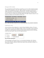
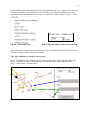
The software operation steps are explained in the following example: First, load an fdi file.
The program will display the network similar to Network Draw (due to a minor bug, the node
coloring is changed). The buttons and controls are located in the bottom right corner (Fig. 51,
highlighted box).
Fig. 51: Layout of Time estimates program
46
Step 1: Click button "Specify ancestral node", then click onto the ancestral node (in Fig 52
example: mv4).
Fig. 52: Calibration step 1: specify ancestral node of known age
Step 2: Click button "Specify descendent nodes" (see Fig 53) and then click all descendent
nodes. To un-select a node, click it again. The selected nodes are coloured green. Due to a
colouring bug, some pie slices are not coloured green correctly. Optionally, median vectors
can also be selected to specify the true tree (if known) within the network.
Fig. 53: Calibration step 2: specify descendent nodes
Step 3: Click button "Calculate time" (Fig 53) and ...(see next page)...
47
Step 4: Calibrate the calculated age (Fig 54) with the known age. For example if the ancestral
node mv4 is known to be 25000 years old, not 59045 years, then the mutation rate needs
adjustment from 1 mutation in 20180 years to 1 mutation in 25000 / 59045 * 20180 = 8544.
Fig. 54: Calculated time.
Step 4: adjust mutation rate to fit known age
After entering the corrected the mutation rate (Fig 54), click the OK button. Then proceed to
estimate the ages of nodes within the network.
2.8.2 Age estimation of a node in the network
Step 1: (example Fig 55), click button "Specify ancestral node", then click onto node OR2.
Step 2: Click button "Specify descendent nodes" and click onto nodes OR1 and OR3.
Step 3: Click button "Calculate time".
Fig. 55: Specify the node for which the age is to be estimated and its descendents
48
The rho age estimation (Fig 56) is independent of demographic parameters. However the
standard deviation is highly dependent on demographic history and the resulting tree shape.
The standard deviation calculation in the example of Fig 56 yields 6976 years (or 0.8165
mutations.
Fig. 56: Estimated age of taxon OR2 and standard deviation in mutations and in years
49
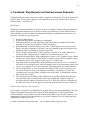
3. Software Limits in Network 4.6.0.0
In the current version, limits are often imposed by memory management rather than available
memory on the PC, which means that a Windows out-of-memory error will occur before the
theoretical maximum number of links or nodes is reached. Some of these limits have been
extended in 4.6.0.0. - Please notify us if you run into a limit (see chapter 5).
Network Data Editor:
Data lines (taxa, sequences):
Data columns (characters, loci, nucleotide positions):
Frequency:
3000
1000 *
999
rdf files from DNA Alignment:
Data lines (taxa, sequences):
Data columns (characters, loci, nucleotide positions):
Frequency:
30000
5000
999
Network Calculations:
Data lines (taxa, sequences):
Data columns (characters, loci, nucleotide positions):
Nodes (haplotypes, median vectors):
Links:
30000 *
5000 *
40000 *
500000 *
* Note that data from Y-STR (ych format) files can lead to locus splitting and very complex
networks. The practical limit for the number of loci may therefore be reached at 500 loci or
less, depending on the number of STRs involved. For RM calculations, limits are much lower
than for MJ or RM-MJ calculations, e.g. for typical RM calculations ca 1500 taxa.
Network Draw:
Max number of mutations displayed on a link:
Max number of links:
200
10000
Mismatch Distribution Tool:
Max distances:
100
50
4. Network 4.6.0.0.: Present and Future
Network has been freely available since January 2000. New versions are usually released at
the beginning of each year. Some interim releases were made in response to urgent requests.
Although Network includes a data editor and a graphics program, fast-growing data sizes and
enhancement suggestions from our user base motivated the development of two additional
software products which are available for a small fee:
-
DNA Alignment is useful for importing and preparing FASTA files for Network.
-
Network Publisher is useful for producing higher quality network graphics and for
displaying node and pie colours depending on "attributes" (additional information for
each sequence or taxon, defined in the Network Data editor: Phenotype, Geography,
Lineage, and the generic Group 1, Group 2, Group 3 which can be renamed). A
compare tool in Network Publisher helps compare two completed network diagrams
(fdi files) and locate nodes or mutations in very obscured networks.
Implementation of future developments
Extensions to data import for Network will be implemented within DNA Alignment.
Extensions to graphics for Network will be implemented within Network Publisher.
Continued availability of the software should be no problem for the next 20-30 years if user
interest remains.
51
5. Feedback: Bug Reports and Enhancement Requests
Feedback between software users and software suppliers is important. We read all emails and
reply to most. We are always happy to read emails from users who simply wish to express
their gratitude – keep these up.
Bug Reports:
Sometimes a reported problem is not quite clear to us, leading to delays and question/answer
emails going back and forward. So before sending your email to us, please take the time to
check whether you have included all information needed to understand and reproduce your
problem. Checklist for your bug report:
1. Describe what happens.
2. In which module, menu, and button or command?
3. With which data file or with which manually entered data (zip/stuff any file before
emailing, to prevent the possibility of email corruption)?
4. Reproducibility: Does this happen every time, or did it happen after you did certain
things? If it does not happen every time, can you remember what you did before this
happened? Did you manage to reproduce this once?
5. Screen setting reproducibility: Is this a graphics problem? If so, under what screen
resolution does it happen? Does it happen at a resolution of 1024 x 768?
6. Hardware Reproducibility: What computer did you use (CPU, graphics chipset, RAM
memory size, free memory on hard disk)? If you have more than one computer: Does
this happen only on one computer or do you see it on others too?
7. Operating-system reproducibility: What operating system did you use? ? If you have
more than one operating system: Does this happen only on one operating system or do
you see it on others too? Are you running the operating system in a virtual machine?
8. LAN-reproducibility: Is your computer connected to LAN (wire or wireless)? If so,
were you working on your own computer's hard drive, or partially over the LAN
(reading from a non-local folder, writing to non-local folder, or running the software
from a non-local folder)?
9. User-privileges reproducibility: Did a different user log into windows with different
user privileges and everything worked, then you logged into windows with your
privileges and the software would not work? If so, does the software work again for
the other user when he or she logs into windows again and tries to use the software?
Enhancement requests ("user wishes"):
We are happy to include your enhancement requests into our bug tracking databases. We will
assign your enhancement requests to Network, DNA Alignment, or Network Publisher.
If you would like us to program a specific enhancement within a specific time frame on your
organisation's budget, please mention this in your email. Otherwise we will simply add your
enhancement request to our list.
Contact: Network development team,
nw [at] fluxus-technology [dot] com
52
6. Updates to the Network 4.6.0.0 User Guide
(Compared to the Network 4.5.1.6 User Guide of 31 December 2009)
1. Modified flow chart Fig 1a in chapter "2.1 Overview of the general work flow and the
RM-MJ work flow": Added “For rooting, use MJ method.”, to reflect the new External
rooting feature in the MJ calculation.
2. In chapter “2.1.5 Epsilon (in MJ), Connection Cost / Greedy FHP (in MJ)”, added 2
sentences that epsilon-values of 0 or 10 are generally recommended. (To avoid
misleading impression that higher epsilon values are generally recommended.)
3. In chapter “2.2.2 Network calculation using the MJ algorithm with optional external
rooting”, added the heading “Calculating the initial network”, and added the new
section “Rooting the network, ancestral node, root proxy node” to reflect the the new
External rooting feature in the MJ calculation.
4. In chapter “2.2.3 Discussing, analysing, and interpreting network results (MJ and
RM)”, deleted the paragraph on rooting and ancestral node.
5. In chapter “2.2.4.1 Node and pie chart colouring in Network Publisher 1.3.0.0”, added
that attributes can be imported into Network Publisher from Excel or a csv file.
6. In chapter “4. Network 4.6.0.0.: Present and Future”, added that Network Publisher’s
Compare tool includes a feature to search for nodes and mutations in a complex
network,
7. In chapter “5. Feedback: Bug Reports and Enhancement Requests”, added operating
system running inside a virtual machine.
7. Updates to Network 4.5.1.6 User Guide (Compared to Network 4.5.1.0 User
Guide of 27 December 2008)
8. Modified flow charts in chapter "2.1 Overview of the general work flow and the RMMJ work flow": In both flow charts (general work flow / RM-MJ work flow), the
sentence "MP can sometimes take several days" is deleted, because this is no longer
the case. In the second flow chart (RM-MJ work flow), the new RM option "no out
file" is mentioned, and the recommendation to try different values of reduction
threshold r is deleted.
9. In chapter "2.1.6 Reduction threshold r and out file option (in RM network option)",
there is a new checkbox option to deactivate step 2 of the RM from calculating links
for an out file. With an explanation of the reason behind this option.
10. Added chapter "2.8 Time estimates".
11. In chapter "3. Software Limits", added note that many memory management limits
have been extended in version 4.5.1.6.
12. In chapter "4. Network 4.5.1.6.: Present and Future", added note on new diagram
compare tool in Network Publisher.
8. Updates to Network 4.5.1.0. User Guide (compared to Network 4.5.0.1 User
Guide of 24 June 2008)
53
1. Exchanged Figs 39-41 for the slightly modified pictures of Network 4.5.1.0 and
Network Publisher 1.1.0.6.
2. In chapter 2.2.4.1 "Node and pie chart colouring in Network Publisher 1.1.0.6", the
old names for taxon attributes / color schemes ("Ethnic Group, Region, Haplogroup")
are replaced (by "Phenotype, Geography, Lineage", and 3 new color schemes are
available which can be renamed).
9. Updates to Network 4.5.0.1 User Guide (compared to Network 4.5.0.0 User
Guide of 31 December 2007)
1. Added RM-MJ calculation for network complexity reduction in chapters 1.3 "Further
Complexity reduction options", chapter 2.1 "Overview of the general work flow and
the RM-MJ work flow", new chapter 2.1.10 "RM MJ calculation", chapter 2.5.2 STR
"Network calculation, analysis, interpretation, and graphics", chapter 2.6.2
Endonuclease (RFLP) data "Network calculation, analysis, interpretation, and
graphics", chapter 2.7.2 Binary data "Network calculation, analysis, interpretation, and
graphics".
2. Added note on human Y-STR 389I and 389II loci in chapter 2.5.1 "Data entry".
3. Added general notes, and added new limit for Network Draw, in chapter 3 "Software
Limits in Network 4.5.0.1".
4. Split Fig.1 into Fig.1a "General overview of the work flow" and Fig.1b "Specific work
flow for the RM-MJ network calculation".
5. Inserted Fig 28, and renumbered Figs 28-49.
6. Exchanged Figs 2, 3, 9, 10, 32, 33, 39, 41, 43-46, 48-50 for the slightly modified
pictures of Network 4.5.0.1 and Network Publisher 1.1.0.4.
10. Updates to Network 4.5.0.0 User Guide (compared to Network 4.2.0.1 User
Guide of 19 September 2007)
1. Changed name length limits in 2.1.2 "Preparation of variable data sets for Network"
2. Changed instructions on entering and saving STR weights in chapter 2.1.3 "Weights"
and in chapter 2.5 "STR data (short tandem repeat, microsatellite data)"
3. Added sub chapter 2.1.7 " MP option to clean up networks "
4. Added sub chapter 2.1.8 "Star Contraction option: Use for network simplification, or
for identification of population expansion events"
5. Added sub chapter 2.1.9 "Frequency>1 Criterion for networks with large number of
taxa"
6. Added instructions for "attributes" entry in the Network data editor, and node/pie
network graphics in Network Publisher, in 2.2.4.1 "Node and pie chart colouring in
Network Publisher"
7. Deleted former instructions about renaming file extensions in 2.4 "Amino acid
nucleotide sequence data "
8. Added notes in chapter 2.5 "STR data (short tandem repeat, microsatellite data)"
9. Changed contact name and email in Chapter 5 "Feedback"
54
10. Several new figures are inserted, many figures are renumbered.
11. Updates to Network 4.2.0.1 User Guide (compared to 3 April 2007)
The following user guide changes on 19 September 2007 were due to an update in the
Network Publisher add-on software, where emf format was added to solve import problems
into MS Office 2003 and newer versions:
1. Added emf format to Fig. 1 "General overview over the work flow"
2. Added emf format to Chapter 2.2.2 "Initial analyses using the MJ option"
3. Added emf format to Chapter 2.2.4 "Graphical Layout of results"