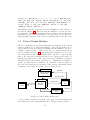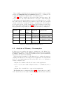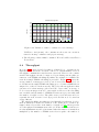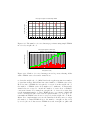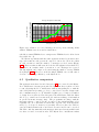
1
Delft University of Technology
Master’s Thesis in Embedded Systems
A Spatial Computing Approach to
Programming Large Scale Wireless Sensor
Networks
Andrei Bogdan Mihoci
A Spatial Computing Approach to Programming
Large Scale Wireless Sensor Networks
Master’s Thesis in Embedded Systems
Embedded Software Section
Faculty of Electrical Engineering, Mathematics and Computer Science
Delft University of Technology
Mekelweg 4, 2628 CD Delft, The Netherlands
Andrei Bogdan Mihoci
[email protected]
30th November 2011
Author
Andrei Bogdan Mihoci ([email protected])
Title
A Spatial Computing Approach to Programming Large Scale Wireless Sensor Networks
MSc presentation
15 December 2011
Graduation Committee
Prof. Dr. Koen Langendoen (Chair)
Dr. Stefan Dulman
Dr. Venkatesha Prasad Ranga Rao
Msc. Ir. Andrei Pruteanu
Mr. Frits van der Wateren
Delft University
Delft University
Delft University
Delft University
Chess
of
of
of
of
Technology
Technology
Technology
Technology
Abstract
The technology required to design and deploy large scale wireless sensor
networks is available, affordable and shows an increased interest in various
application domains. However, application development for distributed systems is a cumbersome task, typically carried out with low–level embedded
programming paradigms. A middleware is usually employed to bridge the
gap between the node–level programming and the overall-system application development. Sometimes, the later one is even performed by non-IT
specialists.
In this thesis we collaborate with the Chess company to integrate the
spatial–computing–paradigm–based Proto middleware with the MyriaNed
production–ready wireless sensor network. We analyze the integration challenges and provide a mechanism that integrates the Myria–specific characteristics (e.g., Gossiping–based communication protocol, Myria Core software design) with Proto. Aditionally, we implement new software modules
(viral code dissemination, target–oriented adjustment of parameters and a
wireless network sniffer for debugging) to enhance the application development process. Finally, we create applications using Myria–Proto to check
the capabilities of the new software stack.
iv
Preface
I would like express my gratitude to the people from Chess who made this
thesis possible and especially to Frits van der Wateren for his support and
guidance every step of the way. I would like to thank Stefan Dulman who
helped and guided me through the entire process. Special thanks go out to
Andrei Pruteanu for his extensive help from the beginning of the project.
I consider myself a very lucky person to have found not only the perfect
supervisor, but a colleague and a friend. I would also like to express my
gratitude to the Proto team for their continuous collaboration and, last but
not least, I would like to thank my family and friends for their support.
Andrei Bogdan Mihoci
Delft, The Netherlands
30th November 2011
v
vi
Contents
Preface
v
1 Introduction
1.1 Problem Statement . . . . . . . . . . . . . . . . . . . . . . . .
1.2 Thesis Contribution . . . . . . . . . . . . . . . . . . . . . . .
1.3 Organization . . . . . . . . . . . . . . . . . . . . . . . . . . .
1
2
3
4
2 Background
2.1 Programming Large Scale Wireless Sensor Networks . . . . .
2.2 Proto Spatial Computing . . . . . . . . . . . . . . . . . . . .
2.3 Discussion . . . . . . . . . . . . . . . . . . . . . . . . . . . . .
5
5
7
9
3 Proto
11
3.1 Proto Simulator and Compiler . . . . . . . . . . . . . . . . . 11
3.2 A Proto Example . . . . . . . . . . . . . . . . . . . . . . . . . 13
3.3 Proto Virtual Machine . . . . . . . . . . . . . . . . . . . . . . 14
4 MyriaNed Platform
19
4.1 Hardware and Communication . . . . . . . . . . . . . . . . . 19
4.2 MyriaCore Software . . . . . . . . . . . . . . . . . . . . . . . 21
5 Implementation
5.1 Architecture . . . . . . . . . .
5.2 Intra–node Communication .
5.3 Inter–node Communication .
5.4 Virtual Machine Extensions .
5.5 Application Dissemination . .
5.6 Network Sniffer And Dynamic
6 Experimental Results
6.1 Applications . . . . . .
6.1.1 Application 1 –
6.1.2 Application 2 –
6.1.3 Application 3 –
. . . . . . .
. . . . . . .
. . . . . . .
. . . . . . .
. . . . . . .
Parameters
. . . . . . .
. . . . . . .
. . . . . . .
. . . . . . .
. . . . . . .
Adjustment
. . . . . . . . . . . .
“all as one“ . . . .
“oscillator“ . . . . .
“firefly and desync“
vii
.
.
.
.
.
.
.
.
.
.
.
.
.
.
.
.
.
.
.
.
.
.
.
.
.
.
.
.
.
.
.
.
.
.
.
.
.
.
.
.
.
.
.
.
.
.
.
.
23
23
25
28
30
31
33
.
.
.
.
.
.
.
.
.
.
.
.
.
.
.
.
37
37
37
38
40
6.2
6.3
6.4
6.5
6.6
Analysis of Memory Consumption
Execution Time . . . . . . . . . . .
Throughput . . . . . . . . . . . . .
Qualitative comparison . . . . . . .
Discussion . . . . . . . . . . . . . .
.
.
.
.
.
.
.
.
.
.
.
.
.
.
.
.
.
.
.
.
.
.
.
.
.
.
.
.
.
.
.
.
.
.
.
.
.
.
.
.
.
.
.
.
.
.
.
.
.
.
.
.
.
.
.
.
.
.
.
.
.
.
.
.
.
.
.
.
.
.
.
.
.
.
.
45
49
53
55
56
7 Conclusions and Future Work
59
7.1 Conclusions . . . . . . . . . . . . . . . . . . . . . . . . . . . . 59
7.2 Future Work . . . . . . . . . . . . . . . . . . . . . . . . . . . 60
viii
Chapter 1
Introduction
Wireless sensor networks consist of small
embedded devices, enhanced with a number of sensors, that are able to communicate wirelessly with each other. Advances
in technology led to the creation of affordable, robust by design and compact formfactors to facilitate the deployment and usage of large-scale wireless networks. One
can imagine in the near future such systems
being deployed in buildings that are not
only able to perform monitoring tasks (e.g., Figure 1.1: Proto Deck tiles
temperature and smoke detection, sensors with sensors and RGB leds.
that measure the force sway during earthquakes, sensors for indoor localization), but also facilitate the interaction
between people. A project that seeks to develop a sensor network platform
that facilitates these new interactions is the Proto Deck lab. at the Delft
University of Technology [34]. The project aims at creating an interactive
environment based on a pressure sensitive floor. The network, built out of
embedded devices with pressure sensors and RGB LEDs attached to each
tile (Figure 1.1) can detect when a human steps on the tiles and react in the
form of light patterns. One other WSN application is to find faulty street
lights in a large section of the Schiphol airport (has over 80000 lights [17]).
The standard methodology is for a person to inform a special public service
if a light is broken. However, especially in an airport, people rarely have the
time to inform the public service.
The challenge of reconfiguring WSNs extends further when the specifications or the applications change after deployment. If a new light show
must be enabled for the Proto Deck, or the light checking application at the
Schiphol airport must be updated, a section or even the entire network must
1
be reprogrammed. This usually implies calling a field specialist to perform
the task and requires a lot of time.
The power of the wireless sensor network applications relies on the scalability of the systems. When programming such networks starting from the
node level, the behavior of the entire system becomes difficult to predict
and, in the end, the application might prove to be un-scalable. The developer must also have a good understanding of the communication protocols
and how they affect the energy efficiency or the memory management at the
nodes (e.g., fair buffer allocation, removal of duplicate network packets etc.).
Programming may prove to be not flexible enough (depending on the underlying hardware platform, the communication channel and the application
requirements) and more suited for people with a thorough multi-disciplinary
technical background (hardware, software and wireless technology). Macro–
programming a spatial computer is a paradigm that seeks to address these
challenges. The goal is to have a high level programming language capable
of specifying applications as global behaviors and to rely on the ability of
a middleware to translate the system behavior of the network into device
actions [27]. New macro-programming languages are more user-friendly
and easier to use and understand by people with no technical background.
Creating an easier to develop platform shifts the focus from low–level technical issues and opens new doors for non-IT specialists that are interested
in developing applications for large-scale wireless networks. Furthermore, it
can also offer a solution to the challenge of reprogramming entire networks
when the specifications change after the deployment.
For this thesis we worked with the Chess Company [11] to determine
the actual capabilities of a merge between their platform and one of the
most popular WSN middlewares called Proto [36]. It relies on the spatial
computing paradigm, and is an ongoing project that unifies the research of
several universities and companies (MIT, Raytheon BBN and TU Delft). To
analyze the performance of the new unified software stack on a real WSN
platform we integrated Proto middleware with Chess’ MyriaNed wireless
technology. We created new software modules and features to improve the
integration and the capabilities of the Myria–Proto platform and created
new applications with the Proto macro–programming language.
1.1
Problem Statement
The goal of this thesis is to determine the capabilities of the Proto middleware in combination with a production–ready wireless sensor technology.
The Proto language that is based on the macro-programming spatial computing paradigm, is designed from ground-up to address the problem of
programming large-scale systems. However, an embedded platform comes
with a set of limitations. The aim is not only to find out the steps that must
2
be taken to integrate Proto with the MyriaNed network, but also to discover the minimum hardware requirements and the challenges a user should
expect outside of the PC simulated environment.
This thesis will answer the following research questions:
1. Are the tools provided by the Proto middleware sufficient for an integration with a wireless sensor network ?
2. If not, what are the challenges a programmer will encounter ?
3. Can Proto execute applications on wireless networks that exhibit low
throughput ?
4. Is it possible to wirelessly replace an application after deployment with
Myria–Proto ?
5. Can Proto virtual machine be deployed on any resource–constrained
embedded platforms ?
1.2
Thesis Contribution
The final goal of this thesis is to attain a functional Proto based MyriaNed
wireless sensor network middleware.
To address the challenges described in the previous section this thesis
makes the following contributions:
• Design and implementation of a intra–node communication protocol
between the MyriaNed software and the Proto virtual machine.
• Design and implementation of a inter–node communication architecture that enables: optimized Proto message exchange between nodes,
application update and reprogramming of different parameters at any
time.
• Design and implementation of a virtual machine execution scheduler
dependent on the application type.
• Design and implementation of a viral code propagation module for
wirelessly reprogramming applications.
• Design and implementation of a terminal command driven sniffer for
data logging and for selectively reprogramming various sensor node
parameters.
3
1.3
Organization
The rest of the thesis is organized as following. Chapter 2 describes the
related work on macro – programming of wireless sensor networks and the
theory behind Proto spatial computing. Chapter 3 gives a short introduction on Proto simulator and presents the Proto virtual machine. Chapter
4 presents the capabilities of the Myria nodes and describes the MyriaNed
software and it’s interaction with the gMAC protocol. Chapter 5 describes
the implementation of the Myria–Proto integration and the modules that
were added to it, while focusing on the encountered challenges. Chapter 6
presents the applications deployed on the platform and an analysis of the
hardware requirements and the performance of the Myria – Proto platform.
We state the final conclusions and give insights of the future work in chapter
7.
4
Chapter 2
Background
This chapter places our work in the context of existing approaches towards
programming large–scale systems work and introduces the theory behind
Proto. Section 2.1 gives a brief introduction to the WSN research that
looks into macro–programming. Section 2.2 depicts the spatial computing
paradigm and the Proto language.
2.1
Programming Large Scale Wireless Sensor Networks
Sensor nodes are low cost, low power devices that combine physical sensing
and communication capabilities to perform a range of tasks, ranging from
monitoring [20] and tracking [21] to building control (e.g., heating, ventilation or air-conditioning) [15]. Developing applications for wireless sensor
networks is not a trivial task due to the diversity of the underlying hardware and various application requirements. Using a middleware layer seeks
to eliminate the gap between high–level application design and platform
dependent low–level programming [30] [19]. The need for a middleware
layer is also emphasized in [31] where the authors describe the fundamental
differences between various state–of–the–art programming approaches for
WSNs by examining various programming language aspects (e.g., programming paradigm, data access model, communication model) and architectural
aspects (e.g., support for high–level application development, low-level configuration such as access to the communication layer parameters, execution
environment–real hardware or through simulations).
A complete middleware solution includes both programming support for
high–level application development as well as the underlying programming
abstractions [19]. The former refers to services and runtime mechanisms
employed for code execution, and services specific to certain platform or ahe
application. The latter focuses on programming paradigms used to describe
network behavior.
5
In [19] the authors identify the main middleware types as: database based
(Cougar [41], TinyDB [24]), virtual machine based (Mate [22], Proto [3],
Darjeeling [9]), modular programming (Impala [23]), application driven
(Milan [32]) and message oriented (Mires [37]). The database–based approach is preferred by most researchers in the field (e.g., Regiment, Cougar,
TinyDB [8]). This type of middleware offers, in general, an SQL–like language that relieves the user from using an embedded C programming query
based architecture [16]. The middleware provides easy access to sensor data,
however, it lacks the support for real–time applications. SORA [26] uses
also a database approach that is now combined with reinforcement learning
techniques. Its main focus is on resource allocation and energy efficiency.
SORA’s programming model lacks the complexity of Proto and is only able
to provide a limited number of primitives for controlling the behavior of the
network. Milan tries to increase the node lifetime by enabling application–
directed network reconfiguration. Similarly to SORA it does not offer an
advanced programming language. The middleware type used by Mate belongs to the same category as Proto, i.e. virtual machine based. However,
at the moment, Mate does not provide a high-level programming language
and programming models required for high–level application development.
The programming abstractions found in the literature can be roughly
separated in two main categories: local programming, used to describe local behavior [35], and macroprogramming (TinyDB, Cougar, Flask [25],
Proto, Kairos [18], Regiment [33]) where operations are defined globally
for the entire network. The Proto middleware implements a model of a spatial computer based on the amorphous medium abstraction [2] and makes
use of a high–level macroprogramming language. While the macroprogramming language is used to write applications that describe global network
behavior, a virtual machine executes on the embedded platform to translate the application program into device actions through local computation
(only the nodes in the neighborhood are taken into consideration). Similar
to Proto’s programming model we find Regiment. However, Regiment still
has underlying problems in adapting the programming model to sensor networks [2]. Another approach to spatial computing is the one based on the
Bayesian network abstraction, a form of probabilistic graphical model [27].
This approach enables the design of networks with support of distributed
analysis of data. The Bayesian network approach is still at an early stage
and, even though it is able to automatically deal with low level networking
aspects, it does not automatically deal with structuring and partitioning of
the Bayesian network, processes that must be manually handled by the user.
Kairos is a programming model that describes global behavior by providing
three programming abstractions:
1. addressing of the nodes,
2. iterating through the 1-hop neighbors of a node,
6
3. reading/writing node values.
The programming abstractions are used to create graph–like structures.
However, compared to Proto, Kairos’ abstraction model does not take into
consideration the geometry of the space in which the nodes are deployed.
As observed also in [31], most middleware–based approaches are evaluated
in a simulated environment. However, real–life deployments and thorough
analyses of the results obtained after the deployment on embedded platforms
are almost absent and the research stops at an early stage without providing
continuous support for the software frameworks or analysis and conclusive
results.
2.2
Proto Spatial Computing
Spatial computing is a computational model in which a program runs on a
collection of devices spread through a physical space [3]. The interaction
between them is strongly dependent on the geometry of the space and the
distances separating the devices. Proto programs describe global network
behavior as an abstraction of the physical space [2]. The spatial computing
approach is based on an approximation of the amorphous medium abstraction. The space in which the nodes are deployed is approximated with
a continuous filling material comprised of individual particles representing
computational devices [1]. The Proto middleware uses a global–to–local
compilation to translate the behavior into device actions.
Figure 2.1: Global abstraction layer comprising Proto libraries that describe
the behavior of regions in the space filled with computational devices [7].
The amorphous medium abstraction bridges the gap between the high–
level application requirements and the device actions on three layers: global,
local and discrete [7]. The global layer (Figure 2.1) represents the Proto
library of programs and algorithms written in the Proto language that describe various aggregate behaviors. The local layer is the approximation
of an amorphous medium where the Proto functional language is executed.
The amorphous medium is a manifold (Figure 2.2) in which every point
7
Local
Figure 2.2: Local abstraction layer represented by the amorphous medium
abstraction as a continuous filled material with computational devices. Each
one can share states to nodes in its neighborhood [6].
is a computational device [6]. All devices run the same Proto programs
and communicate with the neighbor nodes by sharing states. Depending on
the running application, a device can share one state or a field of a state.
The state information propagates through the network at a fixed rate and
the device state is dependent on the information received from all the other
devices in the network.
The discrete layer (Figure 2.3) emulates the amorphous medium by approximating it with a mesh–like spatially discrete network. Each computational device in the mesh is connected to nodes located at distances smaller
than its transmission range. The nodes in the neighborhood communicate
by exchanging state information.
Figure 2.3: Discrete space abstraction layer depicting the topology of the
network. [7]. The layer approximates the amorphous medium by a mesh–
like spatially discrete network.
To better understand how the previously described abstraction layers are
used by Proto, consider a gradient application for the the Proto Deck project
described in section 1. The application creates a gradient whenever a pressure sensor of any node attached to a floor tile is activated. In this case,
the space is represented by the floor and the computational devices are
the sensor nodes in the floor. At the global abstraction layer, the Proto
8
library offers a function/program for creating gradients that can be used
to describe the aggregate behavior. The program is translated into Proto
commands and executed on each device. The devices share with their neighbors state–information on the status of the pressure sensor and the gradient
values. The state information is propagated with a fixed rate through the
network. At the discrete abstraction level, the device holds information
about the neighborhood and nodes coordinates. The information is used to
compute the distances between neighbors and to update the gradient when
a sensor node is activated. Although there are many domain-specific programming models for spatial computing (Abstract Regions [40], Regiment
[33], Bayesian Network [27]), Proto abstraction of an amorphous medium
is a practical tool that copes with many wireless sensor network problems
(e.g., scalability, re-use in terms of algorithms, porting/sharing of libraries
on different platforms, node mobility, prototyping). It offers a powerful abstraction model, an easy–to–use functional language, ongoing user support
and improvements through a continuous development by several research
groups.
2.3
Discussion
A complete solution that addresses all WSNs challenges has been researched
for several years. In this chapter we briefly described state–of–the–art middleware approaches that address these challenges. However, there is no middleware that can offer a complete solution. Some are focused on resource
allocation and energy efficiency, others on providing support for real time
applications or offer an advanced programming language. A crucial aspect
is also the absence of continuity and conclusive results. The middleware approaches surveyed are based on promising paradigms. However, the research
is either stopped at an incipient phase or the middleware approaches do not
seem to provide an infrastructure that will allow continuous additions and
improvements.
The spatial computer paradigm employed by Proto is designed for general distributed systems. The project is still at an incipient phase and its
adaptation to wireless sensor networks is a work in progress. The advantage
Proto middleware has is the foundation on which it is designed, the spatial
computing paradigm and the toolchain it offers. On the Proto foundation is
room to build and improvements can easily be added for any type of system.
9
10
Chapter 3
Proto
Proto is a functional language that is based on the spatial computing paradigm
[3]. It is designed for large scale distributed systems. A complete toolchain
was created to assist a programmer in the application development. The
Proto–toolchain is comprised of three main components: a compiler, an
event–based simulator and a virtual machine that translates the desired behavior into device actions. In section 3.1 we give a brief description of the
first two components. In section 3.2 we exemplify how the simulator and
the compiler are used in the development of an application. In section 3.3
we describe the virtual machine deployed on the Myria embedded platform
[38].
3.1
Proto Simulator and Compiler
The Proto middleware uses a global–to–
local compilation to translate the behavior
Input
5
2
fields
of the network into device actions. The first
two components of the Proto toolchain run
on the PC to create and debug the applicaOperand
tion, simulate the behavior of the network
+
and to generate the Proto script. The outOutput
put script is a description of the application
stream
7
and the input for the virtual machine that
runs on the embedded platform.
The desired network behavior is de- Figure 3.1:
Proto acyclic
scribed with the Proto LISP–like functional graph for expression "(+ 5
language. The language provides a number 2)".
of operands and primitives depicted in [28]
which are used to manipulate streams of fields and to create Proto expressions. A field is a map that assigns the storage of a value to every device in
the network, i.e., an expression equal to an integer is translated into a field
11
holding that integer value at evert device in the network. A Proto expression
is evaluated as a data–flow graph that produces a stream of output values.
For example the Proto program "(+ 5 2)" is translated into the graph in
Figure 3.1 and after the graph is evaluated a stream of sevens will be generated [7]. Proto provides also a number of primitives to manipulate space
and time. These primitives enable the following: space restriction to limit
the space where a code is evaluated, incremental evolution, control over the
rate at which programs are evaluated and field/summary operations [4].
The latter are used to access previously computed values on a device and
to implement the communication. Since Proto approximates a spatial computer (Section 2.2), the number of neighbors a device has can grow infinitely
and the interaction through message passing between nodes is impractical
[3]. In Proto, the communication is enabled by applying field/summary operations over all values in one node’s neighborhood. The values represent
messages from neighbors or the neighbors’ state information as explained in
section 2.2. All values are stored on each device in a neighborhood table
that is assumed to store updated information at all times.
The first task of the compiler is to transform Proto programs, no matter
their complexity, into acyclic graphs. Along with the transformation of code
into graphs it generates optimizations by inlining, folding constant sub–
expressions and removing empty structures [3]. Once the graph is created
the compiler goes step by step through the graph and computes the Proto
script representing a round of execution. The compiler offers also a plug–in
system for platform–specific primitives. The plug–in can be used to extend
the number of device actions that can be expressed by the Proto language.
For example, the Proto language provides three primitives to control red,
green and blue LEDs. However, a platform has also orange and yellow LEDs.
The compiler plug–in is used to extend the Proto language with yellow and
orange primitives. Consequently, if the new primitives are used in a Proto
program, the generated script will hold opcodes for the new LEDs color.
To debug the programs and visualize the behavior of the network, Proto
toolchain provides an event–based simulator. The simulator provides:
• control over the execution of the program;
• options for manual or automatic generation of different network topologies (device distributions in the volume of space in a 2D or 3D plan);
• debugger logs to trace different parameters;
• communication settings;
• a plug–in system that can be used to extend available distributions
and time models or modify the simulated environment [29].
12
The underlying functionalities of the simulator are enabled by creating multiple instances of the virtual machine and by running the output script
provided by the compiler on each instantiated VM.
3.2
A Proto Example
Simulator
Proto Program
Step 1
Compiler
Script Output
Step 2
Embedded
Platform
Step 3
Figure 3.2: Steps taken by a user to program an embedded network.
On an network of embedded devices a Proto application is created in
three steps (Figure 3.2). The first step is to write the program in the Proto
language. For a simple application, in which a switch is used to turn on the
green leds of all neighbors, the Proto program has the following form:
(def turnGreen (src)
(if (< 0 (fold-hood max 0 src))
(green 1)(green 0)))
Figure 3.3: Simulator output for turn leds green application.
In the second step the Proto compiler runs the program, generates the
acyclic graph, prunes it and outputs the following script:
13
script[] = { DEF_VM_OP, 1, 1, 0, 2, 0, 0, 10, 4, DEF_FUN_4_OP,
REF_1_OP, REF_0_OP, MAX_OP, RET_OP, DEF_FUN_OP, 17, LIT_0_OP,
GLO_REF_0_OP, LIT_0_OP, LIT_1_OP, SENSE_OP, FOLD_HOOD_OP, 0,
LT_OP, IF_OP, 4, LIT_0_OP, GREEN_OP, JMP_OP, 2, LIT_1_OP,
GREEN_OP, RET_OP, EXIT_OP };
The simulator runs the script and creates a visualization of the behavior of
the network (Figure 3.3). The user uses the simulator to debug the Proto
program and to ensure that the application is according to the specifications.
In the last step the script is transfered to the embedded devices. The Proto
virtual machine deployed on the embedded platform will execute the script.
3.3
Proto Virtual Machine
The Proto application development starts with a description of the network
behavior with the Proto functional language. Once the application is debugged and the network behavior is visualized in the simulator, the Proto
compiler outputs a script – a list of byte–size opcodes and numerical values (see example in section 3.2). The script is the application code for the
embedded platform. The virtual machine is the only Proto component that
runs on the embedded platform and its role is to interpret the script. To
translate the application code into device actions the VM must be integrated
with platform specific software modules (e.g., communication, sensing) or
specific operating system, if available. To attain the desired behavior on
the embedded platform, the integrated VM executes sequentially all the
commands of the script, in a round based execution model.
R/W data
Platform specific
memory block
New instruction
Call instruction
Read script
Script
Machine
Scheduler
Access stacks
Instruction
Set
R/W data
Virtual memory
block
Figure 3.4: VM Software Architecture
Before giving a detailed description of the supported functionalities and
the architecture of the virtual machine, the following terms are defined:
14
• An opcode represents the address of an instruction.
• An instruction is a routine that performs various mathematical or/and
logical operations, VM specific tasks (e.g., push or pop values from the
stack, fold values, jump to a certain opcode in the script) or platform
specific tasks (e.g., turn on a led, read a switch). A plug-in system is
available to extend the number of platform specific tasks controlled by
the VM.
• A function is a series of instructions that get executed in a certain
order. The execution of a function always starts with a special opcode
(DEF FUN) and ends by returning a value.
The virtual machine is a simple kernel that makes use of a scheduler
and a virtual memory block. The machine scheduler (Figure 3.4 ), the
core component of the VM, handles the ”installation“ of the script and
the scheduling of instructions. The ”installation” creates the application
environment (allocates memory for VM memory blocks, reads the number of
instructions of every application function). The scheduler reads the script,
opcode by opcode, using an instruction counter (similar to the program
counter used by a microprocessor), calls instructions from the instruction
set and reads/writes to the virtual and to the platform specific memory.
Memory Block
Data
Description
The most common data types used by the virtual machine:
1. Number – binary32 floating point numbers.
2. Tuple – an ordered list of any type of data.
3. Address – an address of a function in the byte–code of
the Proto script) or any other type of data supported
by the programming language.
4. Undefined – a value of unknown type.
Array
Stack
A list of data elements with a fixed size.
A LIFO structured linear list with some extra options: stack
size check and index based reading of the elements in the
stack relative to the top or to the bottom of the stack.
Table 3.1: Virtual machine virtual memory blocks
The virtual memory block (Figure 3.5) encloses three types of memory:
data, array and stack (Table 3.1). The latter memory module holds an important role in context saving, task scheduling and execution of instructions
and is comprised of three special stacks (Table 3.2). Two array modules are
15
Virtual Memory Block
Execution
Stack
Globals
Stack
Exports
Array
Environment
Stack
State
Array
Data Type
Address
Tuple
Number
Undefined
Figure 3.5: Virtual memory map.
depicted in Figure 3.5. The first one is the state array used array-storing
by the feedback instructions. A feedback instruction enables control over
the program flow. The second memory module – the exports array, holds
the messages received from neighbor nodes. External access to the virtual
memory is available only before and after a complete round of execution of
the virtual machine.
Stack
Description
Execution
Globals
Environment
The standard stack, used as input/output buffer by almost
every instruction.
Stores globally available data that is preserved through consecutive VM execution rounds.
Used to store temporary variables. The variables are destroyed once the computation ends.
Table 3.2: Virtual machine stack memory blocks
The neighborhood table is a lookup table that stores information about
all 1-hop neighboring nodes. The information is stored in the exports array (virtual memory block) and as node parameters in the platform–specific
memory block (Figure 3.6). The exports array contains neighbor state information. The values stored in the exports array can be destroyed when
the current application is replaced or after a VM execution round. To avoid
resending messages with parameters that are constant or that rarely change,
the values are stored on the platform–specific memory block. For example,
in a static network the coordinates of a node do not change. A node can
16
Neighborhood
Table
Virtual memory block
Platform specific
memory block
Exports Array
Node parameters
Figure 3.6: Neighborhood table memory blocks.
send its coordinates the first time he discovers a new neighbor. The neighbor stores the coordinate information on the platform specific memory block.
The values are always available and are destroyed only when the node that
sent them leaves the neighborhood.
The platform–specific memory block is a shared memory block between
the VM and the platform specific software modules that extend the virtual
memory of the VM. It provides an easy way to exchange information between
the virtual machine and the platform. Furthermore, it is the only memory
block used by the VM where the platform specific software should have write
access. This memory section is mainly used by platform–specific opcodes
additions.
The instruction set module is a database that contains all the instructions
that the virtual machine can execute. The functions associated with the instruction set are the execution block of the virtual machine. The scheduler
reads an opcode, prepares the environment (e.g., saves the current instruction pointer in the stack) and triggers the execution of the actions that are
associated with the opcode by calling the instruction defined by the opcode.
To perform the required task, an instruction can access one or multiple
stacks.
The execution of a new application on
a Proto based platform takes place in two
Install Script
phases. In the first phase, install machine
(Figure 3.7), the instruction pointer gets
the address of the first opcode in the script
DEF_VM
(DEF VM OP). DEF VM OP sets the size of the
virtual memory block (stacks size, state arReturn
ray size, exports size). Once the memory
DEF_FUN
blocks are set the script is read step by step
until all functions defined by the application code are executed. Before exiting the
Exit
17
Figure 3.7: Install Script State Diagram.
first phase the instruction pointer is reinitialized for phase two, machine run (Figure
3.8).
Machine Run
DEF_FUN
Save
Context
Execute
Instruction
RETURN
Exit
Figure 3.8: Machine Run - State Diagram.
A machine run corresponds to a virtual
machine round of execution. The application script defines the device actions with a set of functions. The V.M.
executes all functions sequentially, every execution round, in the order in
which they are defined in the script. If the entire script is read, the V.M.
returns the final computed value and exits. A round of execution does not
take place automatically. The platform software controls when a machine
run is executed.
18
Chapter 4
MyriaNed Platform
In this chapter we describe where we deployed the Proto middleware. In
section 4.1 we present the Myria sensor node hardware capabilities and the
MyriaNed communication model. In section 4.2 we give a brief description
of the MyriaNed software environment and the interaction between Proto
virtual machine and MyriaNed software and communication model.
4.1
Hardware and Communication
The MyriaNed wireless sensor network
[12] is the platform chosen to determine the capabilities of the Proto middleware. The MyriaNode is a wireless sensor node with average hardware capabilities (e.g., memory, transmission range, processing power). It is a low cost, low
energy sensor node developed at Devlab
[13]. It integrates the packet based ra- Figure 4.1: Myria Node Verdio nRF24L01+ from Nordic Semiconduc- sion 3.
tor with the ATXMega128 processor from
Atmel. The radio packet–based chip comes with a ultra low power 2.4GHz
RF Transceiver with a very low energy consumption (13nJ per bit) and
autonomous transmission and reception of messages without processor intervention [14]. The ATXMega128 processor operates on a 32.768kHz
resonator, embeds memory (128kByte Flash memory, 8kByte SRAM, 2kB
EEPROM) and various interfaces [10](e.g, UART, SPI, JTAG). A 20-edge
pin connector is also available for an easy connection of external sensors and
actuators. Furthermore, the Myria Node offers a number of other modules
such as 4 LED indicators, 1 Reed contact or integrated 1/4λ PCB antenna.
The network makes use of a gossiping protocol (a biologically inspired
protocol that spreads information in a network in a virus–like fashion) en19
abled by a gossiping–based medium access controller named gMac [38]. A
broadcast message delivery is used to exchange information between sensor
nodes. A node sends a message and the neighbors that receive the message decide if they should process the information. One of the advantages of
broadcasting is that it can easily cope with node mobility (nodes can change
their neighborhood at any time and exchange information without having
any information about the the new neighborhood). To achieve this, MyriaNed makes use of a “Locally Asynchronous Globally Synchronous“ (LAGS)
communication architecture [39]. All nodes in the neighborhood are tightly
synchronized, while at device level, processes take place asynchronously.
Com.
Process
Com.
Process
Com.
Process
…............................
Application Time
Figure 4.2: Execution model of an application on the MyriaNed platform.
Each interval depicts the communication period and the processing period
(message processing and application execution).
For the MyriaNed platform the application time is divided into intervals of
equal length. An interval represents a round of execution in which messages
are received, processed and transmitted (Figure 4.2). All intervals are synchronized and they always start with the communication period. This period
is divided in a number of virtual frames. For energy conservation reasons,
a frame scheduler sets only one active frame in each interval. In Figure 4.3
a communication model is depicted with 3 virtual frames in which a frame
scheduler sets the active frame in every communication period (period 1 –
frame 1, period 2 – frame 2, period 3 – frame 3).
Figure 4.3: gMac frames scheduling [38].
A frame is dived in a fixed number of slots. A slot scheduler assigns every
slot to a timing event (receive, transmit or idle) [38]. An active frame holds
receive slots. The transmit event can be assigned to any slot in the virtual
frames. The end result of this communication model is a backbone for a time
20
division multiple access (TDMA) channel for which various communication
algorithms are available in MyriaNed (e.g., TDMA with static allocation of
slots, slotted Aloha). Furthermore, new TDMA models can be defined by
the programmer at any time.
4.2
MyriaCore Software
Myria Core is a simple kernel that is integrated with the gMac access control layer. It provides an easy way to modify MAC parameters (e.g., frame
size, number of slots, TDMA scheduling strategy). It schedules the application code and calls various communication tasks (e.g., neighborhood
synchronization, scheduling of frames and slots) [38]. While gMac controls
the execution time of the main tasks the Myria Core performs, the simple
kernel provides an interface for the application development.
Frame
Transmit message
gMac activity
appEvalRxMsg
gMacTdmaStrategy
gMacSynchronize
appPrepareTxMsg
← import received messages
← scheduling of frames and slots
← neighbourhood synchronization
Proto VM Run
← run application and prepare next message to transmit
sleep
Figure 4.4: The interaction between gMac, Myria Core and Proto virtual
machine at frame level [38].
gMac divides the application time in fixed size intervals (a frame in Figure
4.4). Every frame starts with a communication period in which new messages are received and the state update message computed in the previous
frame is sent. When a new message is received in one of the available TDMA
slots, Myria Core calls appEvalRxMsg. In the Myria–Proto integration, this
section is used to update neighbor states in the virtual memory. Once the
active communication period ends, the Myria Core scheduler calls gMac to
compute the TDMA strategy for the next frame. To avoid possible time
drifts, the network synchronization is checked at every frame. The unused
frame time can be allocated to execute the application. To achieve this,
Myria Core will call in every frame the appPrepareTxMsg. This time inteval is used to run the virtual machine and prepare the next state update
message that will be transmitted.
21
22
Chapter 5
Implementation
The Proto virtual machine is the middleware component that runs applications on the embedded platform. The Proto toolchain provides the tools
necessary to program various systems, from static wireless sensor networks
to swarms of robots [5]. The VM offers basic functionalities for any Proto
application, independent of the embedded platform that is deployed on.
The programmer in-charge with the integration of Proto on the embedded
platform must extend the VM functionalities and design a Proto based embedded platform able to fulfill all system requirements.
In this chapter we describe the implementation of the Proto based MyriaNed wireless sensor network platform. In section 5.1 we present the basic
interaction between gMac, Myria Core and the Proto virtual machine. Section 5.2 gives a detailed description of the the communication model between
Myria Core and Proto VM, the virtual machine scheduler and the operating
modes of Myria–Proto. In section 5.2 we describe the module that handles the communication between nodes and its interaction with the virtual
machine scheduler. Section 5.4 depicts the additions brought to the virtual
machine in terms of opcodes and the adjustments made to the execution
of the virtual machine on the MyriaNed wireless sensor network. Section
5.5 describes the uploading/downloading of applications and in the final
section of this chapter (5.5) we present our implementation of a sniffer for
MyriaNed. The sniffer is able to log information about the network and to
modify various node parameters.
5.1
Architecture
Applications for MyriaNed wireless sensor network are developed by incorporating the Myria Core software. As explained in section 4.2, Myria Core
is a simple kernel integrated with the gMac access control layer. gMac is
the timing master of Myria Core. It divides the application execution time
into synchronized frames of equal size and it provides a communication
23
infrastructure suitable for various TDMA strategies. Myria Core schedules gMac processes (gMacTdmaStrategy – computation of TDMA strategy,
gMacSynchronize – calls the routine for node’s synchronization) and a fixed
number of processes used by applications (appEvalRxMsg – evaluate a received message, appPrepareTxMsg – execute application, enter sleep mode)
(Figure 4.4).
The Proto virtual machine is
integrated with the Myria Core
gh
Hi
software.
In the Myria–Proto
l
gMac
ve
implementation, Myria Core is
le
y
t
i
r
MyriaCore
o
i
the master of the VM (Figure
Pr
5.1).
It controls the execution
w
Proto
time of the virtual machine and Lo
the receiving of neighbor messages. The VM interacts with Myria Figure 5.1: Priority Levels in Myria–
Core through appEvalRxMsg and Proto.
appPrepareTxMsg as any other application designed for MyriaNed. Since gMac controls the scheduling, all
processes must fit in one frame. In addition to dispatching the virtual machine execution, Myria Core also restricts the execution time of the VM.
timer
Proto VM
Scheduler
VM
execution
Send VM
State
Sensors
Read
Trigger
VM
Application
Read value
Actuators
Trigger
Send VM
State
Myria Core
Scheduler
Install
gMac
Neighbor
Messages
Replace &
Load
Evaluate
Figure 5.2: Myria–Proto Architecture
Figure 5.2 depicts the basic interaction between gMac, Myria Core and
Proto. Timers are used by gMac to enable the “Locally Asynchronous Globally Synchronous“ communication between nodes. Myria Core, controlled
by gMac, schedules the processing of new neighbor messages and the execution time of the virtual machine scheduler. The Proto VM scheduler
24
module (see Section 5.2) handles I/O information, neighbor messages, sets
the VM application and controls the execution of the virtual machine. The
sensor readings can interrupt the execution of the VM at any time. The VM
execution has control over actuators, if available.
5.2
Intra–node Communication
The Proto virtual machine is designed to be independent of the system on
which it executes. When integrated with a wireless sensor network, a mechanism is required to provide the VM with information about the neighborhood and to control platform specific actions (e.g., read sensors, control
LEDs, read buttons and switches status, compute transmission range). The
Myria Core software provides the means required to accomplish these tasks.
However, the virtual machine and the embedded software platform must
continuously exchange information. Even-more, one module must not limit
the functionality of the other. For example, consider the sense opcode in
Proto. The sense is ON when it returns a value of 1. The sense can be turned
ON by activating the switch and also when a neighbor explicitly broadcasts
a message holding a request to set the sense status to ON. The Proto virtual machine does not make the difference between a platform request and
a neighbor request. A neighbor sends a message containing a request to
set the sense status to ON. However, after the node evaluates the received
message and sets the sense status, the virtual machine executes the read
switch instruction corresponding to the sense opcode and sets the sense to
OFF. The instruction overwrites the previously set status value. To address
this problem the platform software module must explicitly communicate to
the VM the sense value and its source.
The execution model of the Proto based MyriaNed platform is divided in
three main tasks: platform–related processes, virtual machine execution and
virtual machine scheduler. The first module encloses all processes besides
the VM scheduled execution (load/upload new application, reply to sniffer
request, I/O and radio events). The second refers to a round of execution of
the virtual machine, a machine run. The intra–node communication employs
a shared memory communication model to enable exchange of information
between modules. The exchange of information has various purposes:
1. synchronization of the virtual machine execution rounds – Nodes communicate with each other by sharing states (see Section 2.2) computed
by the virtual machine. The synchronization of the virtual machine
execution rounds controls the messages broadcast-ed and processed by
a node. It ensures that nodes for which the VM scheduler inhibited the
VM execution and new nodes that joined the network, broadcast their
state information after the virtual machine processes the neighbors
data.
25
2. read/write access to node basic information (coordinates, transmission
range, switch status, LEDs status);
3. input for the VM scheduler.
The data is stored into the platform specific memory block (Section 3.3).
The latter module, the VM scheduler, employs a priority based scheduling
approach to control various operating modes of Myria–Proto.
State Name
Description
CONSUMED
The available messages are consumed (processed by the VM).
RX
A new message was received from a neighbor.
MORE EXPORTS
The message sent was bigger than the size of
the message payload.
NEW NODE
IO
A new node has joined the neighborhood.
An I/O event occurred.
SKIP RUN
SCRIPT TRANSFER
ASK FOR SCRIPT
VM RESTART
The virtual machine execution is inhibited.
A script upload/download is currently taking
place.
Request the new application script.
Restart Myria Core and implicitly the virtual
machine.
Table 5.1: Virtual machine scheduler states
The Myria–Proto operating modes are defined by the states of the virtual
machine scheduler (Table 5.1). Platform related processes and the virtual
machine make use of a message queue holding states of Myria–Proto operating modes. The virtual machine scheduler enters the state with the highest
priority (Figure 5.3) in the message queue and enables the operating mode
defined by that state. If the message queue is empty the scheduler enters
CONSUMED state. The states control the program flow. They decide
if a machine run should take place, set the message type to be transmitted (see Section 5.3) or compute a new message type if a virtual machine
26
execution round took place. Furthermore, the VM scheduler controls the
uploading/downloading of new applications.
We have extended the operating modes of Myria–Proto through a number
of parameters. At the moment, there is no compiler support that generates
a script with opcodes that can modify the value of the parameters and the
values must be set manually. The user can enable the following parameter–
based Proto modes:
1. Continuous – The virtual machine runs every round if an application
script is available.
2. Updated Message – The execution of the virtual machine will use only
neighbor information received in the current round.
3. Listen – Defines the number of rounds a node should listen for neighbor
information without sending any new messages (it sends the same
message each round). If Listen value is set to n, no new information
will be loaded in the transmission buffer for n rounds. New computed
messages are saved in a buffer and are sent after the listening period.
If the application computes more than one new message the listening
period time, only the newest message will be stored in the buffer and
broadcast-ed when the listening period ends.
Priority Level
The parameter values are used to help Myria–Proto
cope with low network throughput and to increase
High
nodes energy efficiency. For example, Updated MesVM Restart
sage mode is used for applications in which the Proto
Ask for script
states change frequently. Due to communication reasons, a node receives messages only from a percent of its
Script transfer
neighbors each round. Consequently, the information
Skip Run
it has about its neighbors is mostly not updated. By
I/0
enabling the Updated Message mode, the Proto virtual
New Node
machine will take into consideration only the state of
nodes from which it received a message in the current
More Exports
round of execution. In the Continuous mode the virRX
tual machine is executed every round. The continuous
Consumed
execution provides background computation required
Low
by many applications. However, there are applications
in which the Myria node rarely processes information Figure 5.3: States
(i.e., a node wakes up only when a sensor is activated, priority in the
processes the information and sends a message to its virtual
machine
neighbors). By disabling the Continuous mode the VM scheduler.
execution is event driven. It is enabled only when an
I/O interrupt occurs or a message is received. The node will spent most
time in idle mode and saves energy.
27
5.3
Inter–node Communication
MyriaNed employs various TDMA strategies to exchange messages between
nodes. At the beginning of each frame, for each message received, a call to
appEvalRxMsg is made. Also, the information found in the fixed size transmission buffer is broadcast-ed to neighbors. The communication packets
hold various information depending on the Myria–Proto operating mode and
the outcome of the virtual machine execution. Each message type defines
the type of information it holds (Table 5.2). The inter–node communication
module stores the message information in the virtual or platform–specific
memory block and prepares the message that will be sent at the beginning
of next frame.
Message Type
Description
UNDEFINED
Unknown message type or message type identical to previous one.
BASIC
Basic information about nodes (coordinates,
global time, application name, transmission
range).
EXPORTS
SNIFFER REQUEST
NEW SCRIPT REQUEST
SCRIPT
Proto state information.
Message sent by the sniffer in order to modify
certain parameters (at the moment for coordinates, global time and transmission range).
Request new application script.
Application script packets.
Table 5.2: Message types in Myria–Proto
The data packet has a direct influence on the virtual machine scheduler.
The inter–node communication module decides for every received message
in which state the VM scheduler should enter and adds the state in the
message queue. If required it enables the execution of the virtual machine
or a transfered script and, it sends to the inter–node module the message
type that should be loaded in the transmission buffer.
For example, Figure 5.4 depicts the interaction between the VM scheduler
and the inter–node module in normal operating mode (all nodes run the same
application). At power up, Myria Core loads the application script from the
EEPROM in the virtual machine. The VM Installs the script and Myria–
28
Received
Basic info
Received
Exports
Store data &
Set VM state
Virtual machine
scheduler
Load
Application
Skip
Run
New
Node
RX
More
Exports
Consumed
Send
Exports
Send
Previous
Message
Load message
Send
Basic info
Figure 5.4: Interaction between the VM scheduler and the inter–node module for normal execution of Proto application.
Proto broadcasts for a predefined number of rounds a Basic message (see
Table 5.2). The VM enters Skip Run mode (see Table 5.1) and broadcasts
the Basic message multiple times. In an ideal setup a message can be sent
only once. However, due to low communication throughput not all nodes
in the neighborhood will hear the new node that joined the network in the
first round. The message is sent multiple times to insure that all neighbors
receive the information. When a neighbor receives a message from a new
node, it enters the New Node state. In this state, the neighbor continues
executing the VM. However, the message that it broadcasts will contain the
“basic“ information no matter the outcome of the VM execution. Once every
node in the neighborhood received basic information about all neighbors,
Myria–Proto enters normal execution mode. The inter–node communication
module checks the message computed by the virtual machine (“Exports“
message), loads in the gMac transmission buffer the new export values and
adds the VM scheduler state for the next round in the scheduler’s queue. The
new VM state can be either More Exports (if the export values size is bigger
then the size of the transmission buffer) or Consumed if all exports are sent.
In the following round the inter–node communication module evaluates the
received messages from the local neighbors. If a message is received, the
new information is stored in the virtual or platform memory and the new
VM scheduler state is added to the message queue. If no message is received
the VM enters Consumed mode. If the Continuous mode is enabled, the
virtual machine is executed. Otherwise, Myria Core sets the node in sleep
29
mode and continues sending the previous computed message found in the
gMac transmission buffer.
If the VM scheduler is designed to enable multiple operating modes at
node level, the inter–node communication is designed to enable global network behavior for various operating modes. It allows nodes at different
locations in the network to run in different operating modes. For example,
a Proto application runs on the Myria network. A new node enters the
network with an old application and asks its neighbors for the new script.
The nodes that received the request enter SCRIPT TRANSFER state and
broadcast the required script packets. All other nodes in the neighborhood
continue the normal execution of the Proto application (see Section 5.5).
5.4
Virtual Machine Extensions
The virtual machine extensions are divided in two parts:
1. VM opcodes (Table 5.3).
2. VM execution adaptation for MyriaNed.
The first defines procedures (instructions) required by the virtual machine
to run Proto applications. The instructions control device actions (sensors
and actuators) and extract network information (e.g, neighborhood density, neighbor id, time distance) by interacting with the platform–specific
software modules. As explained in Section 3.2, the virtual machine input
is a script (a list of opcodes representing the address of an instruction).
We have increased the number of instructions contained in the instruction
set of the Proto VM (see Section 3.3) and we have attached to each instruction an opcode. Some opcodes/instructions are required by the Proto–
compiler/simulator (e.g., HOOD RADIUS, COORD, DT) and others are
platform–specific(e.g., SWITCH, YELLOW).
The second part represents adjustments made to the virtual machine execution to run on the MyriaNed wireless sensor network. The VM scheduler is the component that controls the round base execution approach of
the virtual machine by interacting with the environment and nodes in the
neighborhood. In the VM kernel some small adjustments were made to integrate the parameter–defined Myria–Proto modes (Section 5.2). The main
modification addresses the communication infrastructure of the virtual machine. The usage of the exports array (buffer that stores messages from
neighbors) was modified to cope with low communication throughput. It
allows the VM to work only with a section of the network when data from
all nodes in the neighborhood is not available. This Myria–Proto operating
mode is manually enabled by the user by activating the Updated Message
parameter–based Proto mode. We have modified Proto basic opcodes that
30
process exports value (fold hood and fold hood plus) to discard not updated information and process only the export values received in the current
frame. Furthermore the Listen parameter–based Proto mode can be manually set by the user to inhibit the execution of the virtual machine for a
fixed number of rounds. While, the virtual machine is not executed the
nodes continuously send the same message in consecutive frames and the
percentage of neighborhood information received by a node increases.
5.5
Application Dissemination
The management and maintenance of applications after deployment on wireless sensor networks is a challenging task. Manual re-programming of each
node is time consuming and the challenge increases even-more when the
nodes are deployed in an area difficult to reach. The Proto compiler generates scripts (a list of one byte opcodes) to define an application for the
embedded platform. Changing the application implies replacing the application script.
In the Myria–Proto implementation, we implemented a transfer–script
module to wirelessly replace applications. Each application has one byte
ID. The byte represents a time stamp (month, day, hour and 2 bits are used
as a counter for defining the year). We choose a time stamp for the ID to
simplify the script transfer process. New nodes can join a network with a
different application than the current one. A new application can be diffused
just by encoding the program time in the application ID.
A copy of the application script is always stored on the EEPROM. We
choose to run the application directly from the SRAM to decrease the processing time of the virtual machine. The Myria node has enough SRAM
to store large Proto application scripts (see Section 6.2). In case of node
reboot the transfer–script module loads the newest application into SRAM
(replaces the current application script found in SRAM or loads the one
stored on the EEPROM).
At program time the user can choose between two operating modes:
• Join The Network,
• New Application.
In the first operation mode, a test application with ID 0 is loaded into
SRAM and the script that is stored on the EEPROM, if any, is deleted.
The node will join the network and will broadcast its “basic“ information
(Figure 5.7). The neighbors that receive the message will notice that one of
their neighbors stores a test application and will automatically start sending
the new script. Otherwise, the nodes wait until they receive a message from
their neighbors. Afterwards, it checks the application ID of the neighbor
and requests the application script.
31
Any other
Type of
message
New Script
Request
Script
Final Packet
Store data &
Set VM state
Virtual machine
scheduler
Load
Test
Application
Skip
Run
Ask for
Script
Script
Transfer
VM
Restart
Load message
Basic
Information
New Script
Request
Script
Figure 5.5: Script Transfer Module – States for nodes requesting a new
application (yellow states depict received messages and gray state broadcasted messages).
Script
Packet Packet Packet
1
3
2
Script Packets Size
First opcodes
…
…
Packet Packet
N -1
N
Next (N - 1) * Payload Size
opcodes
Figure 5.6: The script is split in packets that store script–opcodes (first
packet contains the number of packets the script is split into and the first
opcodes, second packet contains next 18 opcodes, third packet next 18 opcodes, etc.).
Since gMac sets the message size to 32 bytes, each script is split in a
number of packets smaller or equal to the size of the message payload (Figure 5.6). Because of the communication overhead introduced by gMAC
and Myria–Proto, a packet can hold maximum 18 opcodes. A node broadcasts a script request to ask for a packet number of the application–script it
downloads. A new application–script download starts by requesting the first
script packet. The first packet is the only one that stores, besides opcodes,
the number of packets the script is split into – equal to the last packet number or the script–packets size. The value is used by the node that requested
the new application to compute when the script transfer should end. If the
32
last packet is received the node stores the new application into EEPROM
and resets. After reset it will load from the EEPROM the downloaded application. If the requested script is not received in a timely manner (in a
fixed number of rounds) the node will stop the script transfer and will load
the previous application–script. A node that has not yet received the entire
application is also able to reply to a script request by sending packets it
has already received. The strategy increases considerably the dissemination
speed of a new application in the network.
Basic
Information
New Script
Request
Store data &
Set VM state
Virtual machine
scheduler
Load
Application
Store on
EEPROM
Skip
Run
Script
Transfer
Load message
Send
Basic info
Script
Figure 5.7: Script Transfer Module – States for nodes diffusing a new application (yellow states depict received messages and gray states broad-casted
messages).
The second operation mode is used for new application dissemination
(Figure 5.7). The programmer manually replaces the script and sets the
application ID to the current time. At program time, a copy of the new script
is also stored into EEPROM. The node enters the network and broadcasts
its basic information. Neighbors notice that a newer application is available
and ask for the new script. The node with the new application broadcasts
the same script packet a number of rounds. If in this time it does not receive
any new script packet request it will return to normal execution mode.
5.6
Network Sniffer And Dynamic Parameters Adjustment
A packet sniffer is an essential tool in a wireless network. It allows programmers to asses the behavior of the network via the captured packets and
debug applications. For the Myria–Proto approach we designed a sniffer
module that interacts with the Proto virtual machine and Myria Core to log
33
information about the neighborhood or to adjust various parameter values.
A node enabled as a sniffer communicates through the UART port with a
Linux–based PC. On the PC, to communicate with the node, we have a build
a small application using the Termios terminal driver interface. The module
offers an interactive way to selectively log information about nodes in the
neighborhood on the local machine. The user has a number of operating
modes available:
1. log information about all nodes in the neighborhood;
2. select the node for which data logging should be enabled;
3. select data to be logged (application ID, packet arrival time, exports
values, transmission range, coordinate);
4. select parameters to be modified on the target nodes (coordinates,
global Time, Proto export values) for a chosen node;
5. command driven logging of information (data can be logged continuously or a parameter value for a node can be requested just once).
The PC module gets terminal commands from the user. The commands
enable one of the available modes. The PC sends a request to the sniffer node
integrated with Myria–Proto to listen/send the required network information. The sniffer listens for the messages received from the nodes deployed
in its transmission range and sends back data to the PC module. If a request is sent to the sniffer to modify a parameter on a given node, the sniffer
broadcasts a message with the value to be changed and the ID of that node.
The inter–communication module of the Myria node in question interprets
the message and modifies the requested parameters. The sniffer request is
best effort and the only way to check if the parameters are modified is to
visualize the new set of node values on the PC terminal. The sniffer module
can be used to modify various parameters without reprogramming the node
and has no influence over the execution of the virtual machine scheduler.
For example, it can be used to modify nodes coordinates while the nodes in
the network continue the normal execution of the application. The sniffer
functionalities can be easily extended to any Myria–Proto parameter.
34
Opcodes Name
RED
GREEN
ORANGE
YELLOW
LEDS
SWITCH
SENSE
HOOD RADIUS
NBR RANGE
NBR LAG
NBR BEARING
DT
SET DT
MID
AREA
INFINITESIMAL
NBR VEC
COORD
Description
Turns on/off the red led on the myria node.
Turns on/off the green led on the myria node.
Turns on/off the orange led on the myria
node.
Turns on/off the yellow led on the myria node.
Enables the RGB led and turns the led to the
desired color.
Returns the status (on/off) of the switch (the
switch is on if is continuously pressed).
Makes the switch behave as a button and returns the status (on/off) of the “button“(the
“button“ is on if a transition off - on occurred).
Returns the maximum transmission range of
the node.
Returns the maximum expected range at
which devices can communicate.
Returns a best-effort approximation of the
time distance of the current neighbor.
Returns a best-effort estimate of the location
of the current neighbor in polar coordinates.
Returns the time between steps in evaluating
a program in seconds.
Sets the time step to a fixed desired value.
Returns the node’s id.
Returns an approximation of the broadcasting area of a node using the current enabled
transmission range.
Returns the density of the neighborhood as
the number of neighbors.
Returns a field of vectors to neighbors in local
coordinates.
Returns a tuple holding the node’s coordinates.
Table 5.3: Myria specific opcodes
35
36
Chapter 6
Experimental Results
In the first section (6.1) of this chapter we present the applications we created
for the Myria embedded platform in order to analyze the performance and
the requirements of the Proto–based Myria Core middleware. In section
6.2 we analyze the memory consumption in terms of static memory, code
size and dynamic memory. In section 6.3 we analyze the execution time of
Myria–Proto and in section 6.4 we discuss the communication throughput
of MyriaNed and its influence over the virtual machine execution. The
final section of this chapter (Section 6.6) presents our conclusions about the
experiments.
6.1
Applications
The performance of the Proto–based MyriaNed middleware was analyzed by
executing various Proto applications on the embedded platform. For each
application a program was written in the Proto language and the behavior
of the application was debugged using the simulator. Afterwards, the application script was loaded on the Myria nodes. Due to resource constraints we
were only able to test our applications on small scale networks using a maximum of 20 wireless sensor nodes. Once the script was loaded on the Myria
nodes, we have used the parameter–based Myria–Proto operating modes to
adapt the Proto application to the Gossip–based communication protocol.
6.1.1
Application 1 – “all as one“
The first experiment was based on the embedded C language demo application provided by MyriaNed. The demo is a simple application that makes
use of the switch and the green LEDs available on the Myria nodes. A node
was chosen to behave as a beacon. Whenever its switch is turned ON, the
node activates its green LED and broadcasts a message to it’s neighbors to
trigger the same action. We implemented the “all as one“ application in or37
der to make a comparison between the Proto–based Myria platform and the
usual C-based application developed for MyriaNed. The original C-code is
complex and has a considerable size. The same behavior was also described
with the Proto language. The Proto application–code is simple and can even
be rewritten in one line of code (Table 6.1). The Proto compiler generates a
small–size script of 37 bytes for the Myria node’s virtual machine execution.
Proto Code
Application Script
DEF_VM_OP, 1, 1, 0, 2, 0, 0, 11, 5,
(def allAsOne(src)
DEF_FUN_4_OP, REF_1_OP, REF_0_OP,
(if (< 0 (fold-hood
max 0 src)) MAX_OP, RET_OP, DEF_FUN_OP, 20,
LIT_1_OP, SENSE_OP, LET_1_OP, LIT_0_OP,
(green 1)
GLO_REF_0_OP, LIT_0_OP, REF_0_OP,
(green 0)
FOLD_HOOD_OP, 0, LT_OP, IF_OP, 4,
))
LIT_0_OP, GREEN_OP, JMP_OP, 2,
LIT_1_OP, GREEN_OP, POP_LET_1_OP,
RET_OP, EXIT_OP
Table 6.1: All As One Application
6.1.2
Application 2 – “oscillator“
The second application that we tested was the “oscillator“ application (a
detailed description of the application is presented in [7]). The application
was evaluated on the “Mica2 MOTE“ embedded platform [4]. The Mica2
wireless sensor network was integrated with one of the first versions of the
virtual machine. We run this application on the Myria nodes to asses the
performance of the Myria–Proto implementation and the ability of the new
virtual machine to execute application–scripts generated for previously build
VM versions. Similar to the experiment ran on the Mica2–based WSN, we
have deployed a small–scale static network (18 nodes) and we have assigned
to each node predefined coordinates.
The application creates a sine wave using the nodes RGB LEDs (Figure
6.1). We have placed the nodes on a straight line at equal distances to
each other (location information was available). As depicted in Figure 6.1,
for each X–coordinate there is a corresponding amplitude of the sine wave
and the amplitude corresponds to an RGB LED value/color. The upper
amplitude on the sine wave corresponds to color red, the mid–amplitude
value of the sine corresponds to color yellow and, when the sine wave has
amplitude 0 the RGB LED will turn green. The nodes deployed between
the three–set-point amplitude values on the sine (0, 0.5 and 1) will have a
38
1.2
1
RGB LED value
Turn LED Red
0.8
0.6
Turn LED Yellow
0.4
0.2
0
0
Turn LED Green
5
10
15
20
25
30
35
40
45
Coordinates on X - axis
Figure 6.1: Plane–wave oscillator application.
intermediary color. For example, a node placed between mid–section and
upper sine amplitude will turn the RGB LED to a mixed–red–yellow color.
The oscillation of the sine wave can be triggered by turning on the switch
of any node in the network. The wave will always oscillate in the same
direction, from right to left, for a predefined number of virtual machine
execution rounds.
The application is defined by the Proto code shown in Table 6.2 [7]. It
makes use of 7 user defined primitives/functions (e.g., id – returns the value
of a chosen parameter, maxhops – defines the number of rounds the sine will
oscillate) and a main function (LEDs-osc). The gradient task creates a
time–gradient with the origin in a chosen node (the node for which the
switch is activated). Basically, the time–gradient computes a time value
corresponding to a sine phase for each node in the network. The phase–
value depends on the distance the node is found from the source, distance
which is estimated using the coordinate values we have manually assigned
to each node in the network. The sync--time function is in-charge of the
sine–wave oscillation. It creates a weak synchronization between nodes and
slowly increases the time value corresponding to the sine–wave to obtain
the oscillation effect. The osc task computes the sine value of the node by
taking into consideration the node’s sine–phase and coordinates. The sine
value is used in the main function to assign the corresponding sine–color to
the RGB LED.
The application–script size (128 bytes) for the “oscillator“ is considerably
higher compared to the “all as one“ application. However, the execution
time of the VM on the Proto–based Myria node is very small – between 1.5
and 1.6 ms when the sine oscillation is triggered and approximatively 1 ms
in stand-by mode. The oscillation update value depends on the frame size
and on the network throughput. We have chosen basic Myria node frame
size of 500 ms. The application runs with the Continuous mode enabled (see
Section 5.2) to enable the execution of the virtual machine even when the
sine oscillation is not triggered. Since not updated neighbor information
39
(def id (x) x)
(def max (x y) (if (< x y) y x))
(def min (x y) (if (< y x) y x))
(def maxhops () 999)
(def gradient (src)
(letfed ((n (maxhops) (if src 0 (+ 10 (fold-hood min
(maxhops) (id n) ))))) n))
(def sync-time (src)
(let ((lag (gradient src)))
(letfed ((t 0 (if src (+ 1 t) (fold-hood max 0 (id t)))))
(+ t lag))))
(def osc (src coordinate period)
(sin (/ (+ (sync-time src) coordinate) period)))
(def LEDs-osc (src)
(leds (/ (+ (osc (src) (elt (coord) 0) 5) 1) 2)))
Table 6.2: Proto code – “oscillator“ application [7]
does not have a strong influence over the behavior of the application, the
Updated Message and the Listen modes (see Section 5.2) were disabled.
6.1.3
Application 3 – “firefly and desync“
Synchronicity is the ability of a collection of devices to agree upon a firing
period and a phase. Without having a notion of global time devices communicate to simultaneously trigger actions at precise moments in a fashion similar to fireflies blinking in unison. The WSN synchronicity brings a number
of advantages (e.g., wake up nodes at the same time, increase the energy efficiency, real–time coordination of actions). However, achieving synchronicity
on such networks has proved to be difficult due to node failure, message loss,
communication delays, timing skew.
The “firefly‘ ‘ and “desync“ applications were created to show the influence of the Myria–Proto specific–characteristics (e.g, wireless communication (gMac layer), Myria–Proto operating modes) on the Proto applications.
40
Neighbor Influence
Period
Neighbor
influence time
Node 1
Glow time
Application time
Node 2
VM timer
Application time
Figure 6.2: Firefly Application.
The compiler and the simulator do not take into consideration the characteristics of the WSN platform on which the application is deployed. Even–
though the simulator shows the desired behavior and the compiler generates
a viable script, the execution on the embedded platform mis different. Even–
more, the application with the best performance on the embedded platform
might not depict the desired behavior in the Proto simulator.
The “firefly“ application synchronizes all nodes / virtual–machine–runs
in the network to simultaneously turn on the green LED for a predefined
number of rounds. Figure 6.2 illustrates the “firefly“ application on a network composed of two nodes. The application generates a local timer (the
VM timer in figure 6.2) that splits the application time in LED flash periods.
The VM timer value increases each virtual machine execution round with
( dt) (the time between two consecutive virtual machine runs). At the end
of a period the timer resets and the green LED is turned ON. After glow
time, the LED is turned OFF. Once the timer enters the neighbor influence
period, the node checks the LED status of its neighbors. The timer value
is increased with ( dt) and a value proportional to the number of neighbors
that have the green LED ON.
The convergence of the “firefly“ algorithm implemented depends on the
neighborhood information. Each round of execution a node receives information about neighbors firing phase (the beginning of the period when the
node triggers the LED ON). Depending on the values received the node
slowly adjusts its own phase by increasing the value of the timer. An increase of the timer value translates into a smaller period. Since all nodes
use the same period size, when all neighbors agree on the same period phase
the “firefly“ synchronization is achieved.
The first Proto program for the “firefly“ application is shown in Table
6.3. We have first tested the application in the simulator. The visualized
behavior is the one desired and the compiler generates a viable script. We
add to the “firefly“ application previously described a alpha parameter. The
alpha parameter is used to increase/decrease a neighbor’s influence on the
41
(def fireflyV1 (period neighborTime glowTime alpha)
(letfed ((ticks (floor (rnd 0 period))
(let* ((flash (= ticks 0)) (nbrInfluence (mux (< ticks
neighborTime)
0 (* alpha (sum-hood (nbr flash)))))
(newticks (+ ticks (dt) nbrInfluence)))
(mux (>= newticks period) 0 newticks))))
(green (< ticks glowTime))))
Table 6.3: Proto code – “firefly“ application version 1
local timer and its value can be modified only at deployment. Even-though
the application runs as expected in the simulator, it fails to re-create the
desired behavior on the embedded platform. The simulation takes place
in ideal conditions (all nodes have perfect updated information about the
neighborhood and a node sends a new message at the moment the new message is available). However, in Myria–Proto the message that contains the
status of the green LED is always sent at the begging of the next round. This
introduces one VM execution round delay for each processed neighbor message. Furthermore, due to low communication throughput and non-uniform
neighbor sampling, the virtual machine, at each execution round, receives
updated–node information from a percentage of its neighbor nodes. By enabling the Myria–Proto Updated Message mode (see Section 5.2) the virtual
machine discards not updated neighbor LED information. If disabled, the
erroneous node –information will also influence the value of the “firefly“ local timer . However, nodes continuously form synchronized clusters but not
network–wide synchronization.
To cope with the Myria communication design, we created a new version
of the “firefly“ application in which we have replaced the alpha parameter
with a dynamic parameter that takes into account the number of neighbor
messages processed in each virtual machine execution round (Table 6.4).
As previously described, at the end of a period the local timer resets. At
reset, if the timer value is incresead, due to neighbor influence, with a value
less than ( dt), the neighbors influence on the node’s local timer is lost. To
cope with this problem, in the second version we reset the local timer after a predefined number of periods. Furthermore, in the “firefly“ version
deployed on the Myria nodes (Table 6.5), the VM does not compute the
number of neighbor messages processed. To decrease the execution time of
the VM, we have created a Proto–opcode (see Section 3.3) that uses the
already computed information about the number of messages received in
the current frame by the Myria software modules. Depending on the com42
(def fireflyV2 (period neighborTime glowTime ticksResetRounds)
(letfed ((ticks (floor (rnd 0 period))
(let* ((flash (< ticks (dt)))
(nbrInfluence (mux (< ticks neighborTime) 0
(let* ((flashes (sum-hood (nbr flash))))
(* (dt) (/ flashes (+ flashes
(sum-hood (nbr (= flash 0)))))))))
(newticks (+ ticks (dt) nbrInfluence)))
(letfed(( m 0 (if (sense 1) 1 0)))
(if (< 0 (fold-hood max 0 m))
(rnd 0 period)
(if (>= newticks period) (mux
(= reset ticksResetRounds) 0
(- newticks period)) newticks)))))
(reset 0
(mux (> reset ticksResetRounds) 0
(mux (< ticks (dt)) (+ 1 reset) reset ))))
(green (< ticks glowTime))))
Table 6.4: Proto code – “firefly“ application version 2
(def fireflyV3 (period glowTime neighborTime ticksResetRounds)
(letfed ((ticks (floor (rnd 0 period))
(let* ((flash (< ticks (dt)))
(nbrInfluence (mux (and (>= ticks (dt))
(< ticks (* neighborTime (dt)))) 0
(let* ((flashes (sum-hood (nbr flash))))
(* (dt) (/ flashes (infinitesimal))))))
(newticks (+ ticks (dt) nbrInfluence)))
(if (>= newticks period)
(if (= resetTime ticksResetRounds) 0
(- newticks period)) newticks)))
(resetTime 0
(mux (< ticks (dt)) (+ 1 resetTime)
(if (> resetTime ticksResetRounds) 0 resetTime ))))
(green (< ticks glowTime))))
Table 6.5: Proto code – “firefly“ application version 3
43
munication throughput and due to communication clustering effect (nodes
communicate more often with certain neighbors), on a 18 nodes network
the synchronization can take from 10–15 VM execution rounds up to a few
hundreds.
The final version of “firefly“ (Table 6.6) makes use of the “Locally Asynchronous Globally Synchronous“ communication architecture employed by
Myria Core (see Section 4.1). The application time is already split in fixed–
size periods by gMac. This means that on Myria–Proto you can use discrete time, with the unit equal to the frame width (see Section 4.1). In
this version, the nodes send messages that contain a next–round–VM–timer
estimated value. The synchronization takes place in just a few rounds of
execution (less than 15 in a 19 nodes 2,3–hops network). The Proto code
depicted in table 6.6 is the application code of the final version of “firefly“.
We have added to this program a task to enable the “desync“ routine. When
the switch of a node in the network is turned ON the network desynchronizes
(nodes turn ON the green LED in a random fashion).
(def fireflyDesync (period glowTime)
(letfed((desync 0 (fold-hood max 0 (sense 1))))
(if desync
(letfed ((ticks (floor (rnd 0 period))
(let* ((flash (< ticks (dt))))
(if (>= (+ ticks (dt)) period) 0 (+ ticks (dt))))))
(green (< ticks glowTime)))
(letfed (
(ticks (floor (rnd 0 period))
(let* ((flash (< ticks (dt)))
(nexttick (if (>= (+ ticks (dt)) period)
0 (+ ticks (dt))))
(neightick (fold-hood max 0 nexttick))
(nextneightick(if (>= (+ neightick (dt))
period) 0 (+ ticks (dt)))))
(if (or (and (> ticks neightick)
(or (> neightick (/ period 4))
(< ticks (- period (/ period 4)))))
(and (< ticks (/ period 4))
(> neighTick (- period (/ period 4)))))
nextneightick nexttick))))
(green (< ticks glowTime))))))
Table 6.6: Proto code – “firefly“ application version 4 with “desync‘
44
Due to similar considerations as for the previous “firefly“ version, we have
enabled the Updated Message and Continuous Myria–Proto operating modes
to adapt the application requirements to the Myria system.
Table 6.7 shows a comparison between the firefly versions presented. We
observe that the only version that achieves convergence on the Myria embedded platform in a timely manner is version 4 (“firefly with desync“ ). The
size of the script is considerable bigger than for version 1. However, the final
“firefly“ version also contains the “desync“ operating mode. If the application executes only the “firefly“ synchronization the application–script is 165
bytes. As we will conclude in Section 6.2, Myria–Proto can store and execute
large application–scripts without concerning about memory consumption.
Firefly
Version
Script
Size
Version 1
Version 2
86 bytes
181 bytes
Platform
Dependency
None
None
Version 3
142 bytes
Low
Version 4
237 bytes
High
Convergence
Achieved
on
Simulator
Simulator
and platform
Platform
Simulator
and platform
Platform Convergence Time
Infinite
Random (10 up to a
few hundred rounds)
Random (10 up to a
few hundred rounds)
Less than 15 rounds
Table 6.7: Virtual machine scheduler states
6.2
Analysis of Memory Consumption
In this section we analyze the memory consumption of the Myria–Proto
implementation on three levels: SRAM (memory allocated at program time
in SRAM), FLASH (code size) and dynamic memory (data dynamically
allocated at run–time in the SRAM).
We first run an experiment on the Myria nodes to analyze the memory
consumption differences between the C-based application development and
the Proto–based implementation. We deployed the “all as one“ application
versions on Myria nodes:
1. Myria Core with the embedded C version of the application;
2. Proto–based version without Myria software or communication modules;
3. Myria–Proto with the Proto version of the application.
The SRAM memory consumption (Figure 6.3) depicts an increase of 3.06%
of the .bss memory section (stores uninitialized global and static variables)
45
Size (bytes)
SRAM Usage
1500
1400
1300
1200
1100
1000
900
800
700
600
500
400
300
200
100
0
Myria
Proto
Myria-Proto
.noInit
.bss
.data
Memory Section
SRAM
Figure 6.3: Comparison of SRAM usage for the various implementations(“all
as one“ application).
for the C-based Myria compared to the Myria–Proto implementation. However, Myria–Proto contains more static data that is defined in the code.
The extra memory consumption for this type of data is shown in the .data
section. The Myria nodes that execute only the Proto virtual machine without the Myria software modules store 94.7% of data in the .data section.
The total SRAM memory consumption shows that the memory usage for
the Myria–Proto implementation is higher than 16% compared to the Myria
Core C-based version of the application. The small increase is due to the
fact that Myria software modules and Proto share a high amount of data.
The “all as one“ application on Myria–Proto uses 1.43 kBytes of SRAM
memory out of 8kBytes available. The remaining 6.57 kBytes are used for
the neighborhood table and for storing the application script. Taking into
account that the script size for the all as one application is 37 bytes, the basic SRAM usage for Myria–Proto when the node is isolated from the network
and no application is loaded is only 1.39 kBytes.
The Proto virtual machine increases considerably the code size(Figure
6.4). It uses almost twice as much Flash memory than Myria Core. Myria–
Proto increases the FLASH memory consumption by 3.69 times. It uses
48.61 kBytes of Flash memory. However, the size of FLASH memory on
a Myria node is 128kBytes. The total consumption is less than half of
the FlASH memory of a node. Even–more, the FLASH memory usage is
independent of the size of the Proto application–script (Figure 6.5).
The application–script size influences the SRAM memory usage. A Proto
application of higher complexity makes use of more variables/parameters.
Additionally the Proto compiler generates a larger application–script (more
opcodes). Consequently, on the embedded platform the .bss and .data
SRAM memory sections increase in size. However, as illustrated in Fig46
Size (KBytes)
Code Size
55
50
45
40
35
30
25
20
15
10
5
0
Myria
Proto
Myria-Proto
Flash
Flash+SRAM
Memory Section
Figure 6.4: Comparison of FLASH usage for the available implementations
of “all as one“ application.
Size (KBytes)
Code Size
55
50
45
40
35
30
25
20
15
10
5
0
Flash
Flash+SRAM
14
45
79
135
164
Script Size (number of opcodes)
237
Figure 6.5: Influence of the application size on the FLASH memory usage.
ure 6.6, for a script–size increase of 16.9 times (script size of 14 bytes vs.
script size of 237 bytes) the SRAM memory consumption increases with only
15.36%. The “firefly with desync“ application generates a 237 bytes script.
However, on the embedded platform the application uses only 1.62 kBytes
of SRAM out of 8 kBytes.
The memory consumption for the applications presented in Section 6.1
depict similar results. The application–script size influences only the .data
memory section (Figure 6.7). The largest application (“firefly with desync“)
increases the .data memory section with 29.41% (200 bytes) and the SRAM
consumption is less than 1.7 kBytes. Furthermore, the consumption of all
other memory sections is independent of the application: .noinit – 3 bytes,
.bss – 784 bytes, Flash – 48.61 kBytes.
Our final experiment analyzes the usage of dynamic memory on Myria
47
Size (bytes)
SRAM Usage
2000
1900
1800
1700
1600
1500
1400
1300
1200
1100
1000
900
800
700
600
500
400
300
200
100
0
.noInit
.bss
.data
SRAM
14
45
79
135
165
Script Size (number of opcodes)
237
Figure 6.6: Influence of application size over SRAM.
Size (bytes)
SRAM .data Section Usage
1800
1700
1600
1500
1400
1300
1200
1100
1000
900
800
700
600
500
400
300
200
100
0
All as one - 37 op.
Oscillator - 135 op.
Firefly v1 - 86 op.
Firefly v2 - 181 op.
Firefly v3 - 142 op.
Firefly v4 - 237 op.
.data
.Sram
Memory Section
Figure 6.7: SRAM memory consumption for the applications presented in
Section 6.1. The legend specifies the application name and the application–
script size in number of opcodes.
nodes. In the Myria–Proto implementation, the dynamic memory is defined
by the size of the neighborhood table (see Section 3.3). The neighborhood data is stored in SRAM. The table stores for each neighbor 32 bytes
of basic information (e.g., node id, global time, coordinates, transmission
range) and an exports array (stores the message computed by the Proto
application – see Section 3.3). The size of the neighborhood table increases
linearly and its value in bytes can be estimated with the following formula:
dynamicM emory = neighborhoodSize∗(32+(5∗importsSize)). Figure 6.8
illustrates the increase of the SRAM dynamic memory with the size of the
neighborhood and the number of exports (neighbor states). We observe that
in a dense network (15 nodes per neighborhood) the memory consumption
is less than 800 bytes even for complex applications that require storing for
48
Dynamic Memory Usage
800
700
Size (bytes)
600
500
400
300
200
1 Import
2 Imports
3 Imports
4 Imports
100
0
0
2
4
6
8
10
Number of Neighbors
12
14
16
Figure 6.8: Influence of the number of neighbors and the number of virtual
machine imports over dynamic memory.
each neighbor 4 neighbor states in the neighbor’s exports array (the final
version of the firefly application exports only one state).
The Myria platform has 2kBytes of EEPROM memory. In EEPROM we
store the node coordinates and the application–script. Since the coordinates
have a size of 12 bytes, Myria–Proto can store large application–scripts (sizes
up to 2036 opcodes).
6.3
Execution Time
In Myria–Proto, the application time is split in equal frame sizes (see Section
4.2). The frame size is set at program time. A basic frame size used by
MyriaNed is 500 ms. All processes, including message evaluation, virtual
machine execution and load new message for transmission, must be executed
in one frame.
The virtual machine execution time dependents on the size of the script
and the number of neighbor messages it processes. If the node is isolated
from the network or the virtual machine does not process any neighbor information (e.g., due to communication problems), the time increases almost
linearly with the application script–size (Figure 6.9). However, even for
complex applications with large scripts (236 opcodes for the “firefly with
desync“ application) the execution time is modest (on average 2.34 ms in a
dense neighborhood that contains 18 nodes). If a node joins a dens network,
the virtual machine will process at each round multiple neighbor messages.
However, the execution time does not increase substantially.
For example, Figure 6.10 illustrates the virtual machine execution for
the ‘‘firefly with desync“ application (version 4 – see Section 6.1.3) when
the “firefly“ operating mode is enabled. We have started the experiment
49
Virtual Machine Execution Time
2.14
1.74
Time (ms)
1.52
V.M. Execution Time
0.63
0.2
0.058
14
45
79
135
164
Script Size (number of opcodes)
236
Figure 6.9: Influence of the application size over the virtual machine execution time
Time (ms)
Virtual Machine Execution Time - Neighbor Influence
3
2.8
2.6
2.4
2.2
2
1.8
1.6
1.4
1.2
1
0.8
0.6
0.4
0.2
0
V.M. Execution Time
0
10
20
30
40
50
60
70 80
Rounds
90 100 110 120 130 140
Figure 6.10: Virtual machine execution time evolution for “firefly with
desync“ (version 4 – see Section 6.1.3)application using distributed Aloha
with 16 TDMA slots and 8 virtual slots. We have enabled only the “firefly‘
operating mode.
with a network composed of only 2 nodes. Step by step we have increased
the number of nodes in the neighborhood until we have a created a 1–hop
network of 18 nodes (all 18 nodes joined the network at execution round
number 90 – the X-axis in Figure 6.10). The nodes were deployed using
the distributed Aloha scheduling with 16 TDMA slots and 8 virtual slots
(see Section 6.4). Due to low communication throughput a node receives
at most messages from 7 different neighbors. However, when all messages
are processed by the VM the increase in VM execution time is 0.66 ms.
The virtual machine one–round–execution time is less than 1% of the basic
MyriaNed frame time. To better analyze the influence of the application–
50
Virtual Machine Execution Time - Firefly Application
2
1.8
1.6
Time (ms)
1.4
1.2
1
0.8
0.6
0.4
0.2
V.M. Execution Time
0
0
20
40
60
80 100 120 140 160 180 200 220 240 260 280
Rounds
Figure 6.11: Virtual machine execution time evolution for the “firefly “
application Version 4 without the “desync“ routine using distributed Aloha
with 8 TDMA slots and 8 virtual slots.
Virtual Machine Execution Time - Oscillator Application
2
1.8
1.6
Time (ms)
1.4
1.2
1
0.8
0.6
0.4
0.2
V.M. Execution Time
0
0
15
30
45
60
75
90 105 120 135 150 165 180 195
Rounds
Figure 6.12: Virtual machine execution time evolution for the “oscillator “
application using distributed Aloha with 8 TDMA slots and 8 virtual slots.
script size and neighborhood density on the VM execution time, we have
deployed the same application on a node isolated from the network. Since
in the previous experiment we only enabled the “firefly“ operating mode
and the application can perform two separate tasks (“desync“ or “firefly“
– only one at a time can be enabled by the user – see Section 6.1.3 ), we
have reduced the application script size to 165 bytes, 72 bytes less than in
the initial version, by removing the “desync“ routine. The virtual machine
one–round–execution time (Figure 6.11) is, as expected, lower (on average
1.71 ms). We observe that the plotted values showing the V.M. execution
time of the two “firefly“ experiments (Figure 6.10 and Figure 6.11) describe
similar patterns. However, the isolated node (Figure 6.11) does not process
51
Time (us)
Prepare Message Time
180
170
160
150
140
130
120
110
100
90
80
70
60
50
40
30
20
10
0
1 Import
2 Imports
3 Imports
4 Imports
0
5
10
15
20
25
30 35
Rounds
40
45
50
55
60
65
Figure 6.13: The time it takes to prepare a message for transmission.
messages from neighbors. Consequently, its VM execution time does not
increase considerably and its values are always found in a fixed interval
(between 1.67 ms and 1.73 ms).
Similar results were found for the “oscillator“ application (Figure 6.12).
The nodes were deployed using distributed Aloha with 8 TDMA slots and 8
virtual slots. Since the processing time of a received message is significantly
lower than for the ‘‘firefly with desync“ application, the virtual machine one–
round–execution time for the “oscillator“ application is almost constant (on
average it executes in 1.52 ms).
After the virtual machine execution ends a new message is prepared for
transmission(e.g., the type of message is computed, the new message is
loaded in the transmission buffer, the VM scheduler is prepared for the
next round of execution – see Sections 5.3 and 5.2 ). Figure 6.13 depicts
the relation between the process time required to prepare a new message
and the number of exports values the message stores. We observe that the
process time, even in the worst–case scenario, is less than 0.17ms.
Before the virtual machine executes the application, neighbor messages
are evaluated and stored in the virtual or platform memory block. Figure
6.14 illustrates the average evaluation time of a message. Since the message
packet size is limited to 32 bytes a node can only send at most 4 exports
(node state–information – see Section 2.2) per message. In the worst case
scenario (the message stores 4 imports) the evaluation time of a message is
less than 0.1 ms.
In conclusion, the execution time of all processes employed by Myria–
Proto can be computed with the following formulas:
• ExecutionT ime = Evaluate + V M Execution + P repareM essage.
• W orstCaseExecutionT ime = N umberOf ReceivedM essages∗0.95+
52
Time (us)
Evaluate Message Time
110
100
90
80
70
60
50
40
30
20
10
0
1 Import
2 Imports
3 Imports
4 Imports
0
5
10
15
20
25
30
Rounds
35
40
45
50
55
Figure 6.14: Variation of time to evaluate a received message.
V M T ime + 0.17 (in ms) – the constants are the worst case execution
times for message evaluation and prepare message
• The following condition must be satisfied: W orstCaseExecutionT ime <
F rameT ime
6.4
Throughput
In section 5.2 we have described a number of Myria–Proto operating modes
implemented to enable the execution of the Proto virtual machine on a low
throughput communication wireless sensor network. However, the communication throughput can also be improved by modifying various gMac parameters or the TDMA scheduling algorithm. For example, for a small–scale
network a simple TDMA scheduling is preferable. Figure 6.15 depicts the
average number of messages received by a node in a network composed of 7
nodes that use the simple TDMA scheduling protocol (a fixed TDMA slot is
assigned for each node in the network). The nodes run an application that
generates a broadcast message each round. We observe that, on average, a
node receives messages from 85% of its neighbors. However, the scheduling
is not scalable and the number of TDMA slots increases proportionally with
the number of neighbor nodes. The gMac active period increases and consequently the radio is active for a longer period and the node becomes less
energy efficient.
The usual scheduling algorithm used in MyriaNed application development is distributed Aloha, an extension of the Aloha protocol with a dynamic behavior dependent on the number of neighbors [38]. Aloha provides
35% throughput at maximum network load. In the distributed Aloha version the maximum network load is attained when the number of virtual slots
multiplied by the number of TDMA active slots is equal to the number of
53
Message Reception for Static Simple TDMA
7
Number of Messages
6
5
4
Number of Message for Simple TDMA
3
2
1
0
0
10
20
30
40
50
60
Time (frame count)
70
80
90
100
Figure 6.15: The number of received messages per frame using simple TDMA
in a 7 nodes neighborhood.
Number of Messages
Message Reception for Aloha 8x8
17
16
15
14
13
12
11
10
9
8
7
6
5
4
3
2
1
0
Number of Received Messagess
Number of Neighbors Broadcasting Messages
0
15
30
45
60
75 90 105 120 135 150 165 180
Time (frame count)
Figure 6.16: Number of received messages in a 1-hop network using Aloha
with 8 TDMA active slots and 8 virtual slots.
nodes in the neighborhood. gMAC divides the application time in a number
of equal–size frames. Each frame has a fixed number of TDMA active slots.
However, since a TDMA slot is required for every node in the neighborhood,
the number of TDMA active slots might not be sufficient. Consequently,
virtual slots are created to extend the number of active slots on multiple
consecutive frames. For example in a neighborhood of 18 nodes, if the user
set the maximum number of active TDMA slots to 8 per frame, gMAC will
create 3 virtual slots (the active slots are split in frame i, i + 1, i + 2) to obtain sufficient TDMA active slots for every node in the neighborhood. In the
Myria–Proto implementation we use the distributed Aloha version to adapt
the number of virtual TDMA slots to the number of neighbors discovered
by a node (if a node has 8 active TDMA slots and 12 neighbors, gMac will
54
Number of Messages
Message Reception for Aloha 16x8
21
20
19
18
17
16
15
14
13
12
11
10
9
8
7
6
5
4
3
2
1
0
Number of Received Messagess
Number of Neighbors Broadcasting Messages
0
10
20
30
40
50
60
70
80
Time (frame count)
90
100
110
120
Figure 6.17: Number of received messages in a 1-hop network using Aloha
with 16 TDMA active slots and 8 virtual slots.
schedule 2 virtual TDMA slots to assign active TDMA slots for all nodes in
the neighborhood).
We run an experiment with the same application that broadcasts a message each round in a 1-hop network composed of 16 nodes. We noticed that
at each execution round the number of messages received varies (Figure
6.16). Even at almost full network load the throughput is less than 25%.
Even–more, in certain rounds of execution 1 or no messages are received.
The throughput can be improved by increasing the number of active TDMA
slots (Figure 6.17). However, as in the simple TDMA case, it will cause a
decrease of the energy efficiency of the Myria Node.
6.5
Qualitative comparison
The applications we have described in section 6.1 were created for the Myria–
Proto middleware. On any given embedded platform, they would not be able
to run only using the Proto middleware without integrating Proto with the
embedded platform (creating opcodes to control device actions, design a suitable communication protocol). MyriaNed’s gMac protocol impose a number
of design choices when we have integrated the middleware with the MyriaNode (e.g., round based execution model, wireless exchange of information
at precise moments, message size). The programmer in charge with the
integration has no control over the execution of the virtual machine. Consequently, the one–round VM execution time depends only on the hardware
used (e.g., clock speed, memory access time). However, since the VM executes in a timely manner the round based execution model can be avoided.
The VM could automatically send messages when new data is available and
not after a round of execution ends. The Myria–Proto middleware makes
55
a compromise between energy efficiency and application execution time by
sending a message once every 500 ms (frame size used in our Myria–Proto
experiments) and setting the node in sleep mode a high percentage of the
frame – after VM executed and a new message is loaded for transmission.
The “firefly“ application would converge considerable faster if the VM would
execute continuously (in one Myria frame the VM can execute more than
50 times). However, the energy efficiency of the node will also decrease considerably. For the “oscillator“ application the VM is not required to run
continuously. Even–more, the visual effect we created using the RGB LEDs
(plotting a sine–wave using various RGB colors) would minimize. No matter the embedded platform integrated with Proto and the communication
protocol used, a virtual machine scheduler is required to achieve a desired
trade-off between power consumption and application execution time. We
strongly believe that Myria–Proto attains a good compromise.
All applications presented can also be created using embedded C programming and the Myria Core software. A better resource allocation in terms
of memory usage and execution time can be achieved for all applications in
comparison to our Myria–Proto middleware. However, programming using
embedded C requires in-depth knowledge about embedded programming,
hardware, buffer allocation, communication protocols and is not accessible
to non-experts. Furthermore, the performance of the application strongly
depends on the user’s ability to program in embedded C. Proto adds overhead in terms of memory and execution time but, applications for Myria–
Proto can be created by users with basic knowledge about the middleware.
Furthermore, various optimizations are already made by the Proto compiler.
6.6
Discussion
In this chapter we analyzed the memory consumption, the execution time
and communication throughput of the Proto–based MyriaNed middleware.
The results obtained show that Myria–Proto requires a modest amount of
memory (less than 60kBytes of FLASH for code and around 3KBytes of
SRAM) for most applications. Furthermore, the execution time of Myria–
Proto will never reach the basic frame size of gMac (500 ms) – even for
very large application–scripts deployed in dens networks. The SRAM memory available (8kBytes) and the size of the FLASH (128kBytes) allows the
execution of complex/large applications.
The Proto virtual machine can handle complex operations with limited
resources in a timely manner. Besides resource considerations, the Proto
VM also brings the following advantages:
• fast deployment of applications (see Section 5.5);
• provides an easy to use plug-in that enables the addition of platform–
56
dependent tasks (e.g., read sensors, control actuators);
• has a simple architecture that can be extended (see Section 3.3).
Its main disadvantage is the weak integration with the energy efficient communication protocols usually enabled on wireless sensor networks. Basically,
the virtual machine is the arithmetic logic unit (ALU). It will execute complex operations/tasks and will provide the expected output as long as the
input (the information about the network) is correct. The more dependent
the execution is of the input values, the more Proto VM will fail to generate
the desired output. The trade-off between energy efficiency and throughput
(see Section 6.4) met in a wireless sensor network becomes the weakest link
in the Proto middleware.
In the Myria–Proto middleware a Gossiping–based protocol was provided
(see Section 4.1). We have determined that by creating a suitable architecture (see Section 5.1) the virtual machine can execute various wireless
sensor applications using Myria’s gMac protocol. The drawback is the usage of special Myria–Proto operating modes (see Section 5.2)that have to
be manually enabled by the user. Furthermore, the execution model of the
Proto VM enabled on the Myria platform is different from the one assumed
by the Proto simulator and compiler (the communication is not perfect, the
virtual machine does not run continuously, the exchange of information does
not take place instantly). We were unpleasantly surprised by the fact that
we were no longer able to re-create the behavior visualized in the simulator
on the embedded platform. An application for which nodes require correct
network information in real–time (for example the “firefly“ application),
will execute as expected on the MyriaNed only if the user takes into consideration the Myria–Proto communication protocol and operating modes.
However, writing the applications using the Proto high–level programming
language proved to be faster and easier than using the typical C-based programming.
Proto is an ongoing project and modifications to various components are
made daily. The virtual machine we have integrated was build in parallel
with our integration of Proto with MyriaNed. A new version of the Proto
compiler and simulator is currently build. To improve the efficiency of Proto
on wireless sensor networks (see Section 7.2) we believe that compiler and
simulator support is required (see Section 7.2) . The available compiler
plug–in allows a programmer to add platform–specific actions. However,
we found it difficult to use at this stage. Furthermore, the Proto simulator
provides low debugging capabilities which need to be improved (e.g, error
messages are sometimes difficult to understand, there are no breakpoints or
references to line of code where the error is found). As for any programming
language there is a learning curve for programming in Proto. Even at this
stage, with the issues mentioned, Proto programs can be written fairly easy.
57
The Proto middleware does not offer a solution for the communication or
energy challenges encountered in wireless sensor networks. It provides an
easy way to create and deploy applications. At this stage in the project, we
found Myria–Proto to be a good solution for applications that require heavy
computation and limited communication. Applications that require high
throughput can also be deployed but, the user’s work is heavily increased.
We conclude this chapter by providing a comparison between the three
implementations we have discussed (Table 6.8) – Proto, Myria–Core and
Myria–Proto.
Proto
High–level programming language
Re–use in terms of algorithms
and libraries
Does not require basic knowledge about the underlying implementation
Application debugging tools
State–of–the–art communication protocol
Application dissemination after deployment
Fast prototyping
In–build scalability
Re–use in terms of hardware
(platform independent)
√
√
√
√
×
Myria
Core
×
×
Myria–
Proto
√
√
×
×
×
√
√
√
√
×
×
√
√
√
×
√
√
√
×
×
Table 6.8: Comparison between Myria, Proto and Myria–Proto implementations
58
Chapter 7
Conclusions and Future
Work
Using a middleware to bridge the gap between programming of networks
as single entities and the constituent embedded device is a good solution
for many reasons: fast prototyping, re-use of hardware platforms and libraries, scalability, node mobility, non–standard communication protocols
and programming/debugging tools.
In this thesis we presented a state–of–the–art middleware based on the
spatial computing paradigm. We integrated the Proto middleware with
the MyriaNed wireless sensor network and we determined its capabilities
of Proto as an internal part of a production–ready wireless sensor network
technology.
7.1
Conclusions
Proto provides various tools for programming the behavior on a network
of embedded devices: a high–level macro–programming language, an application debugger, a simulator to visualize the application behavior, a compiler that generates optimized application–scripts, a virtual machine that
executes the generated script on embedded platforms. The programmer in–
charge of the integration of Proto on an embedded platform can use the
virtual machine plug-in to extend the VM functionalities to execute various
device–specific actions (e.g, sensor readings, actuators control). However,
the VM is only the computational block. A mechanism is required to schedule the execution of the virtual machine and to provide information from the
network. The programmer is also in–charge of the wireless communication
design, energy efficiency and resource allocation (e.g, memory, tasks).
The Myria Core software provides the tools required to create the previosly described building blocks for the Proto integration with the Myria
platform. One of the main challenges encountered was adapting the virtual
59
machine execution to low throughput wireless communication. By creating
various operating modes for Myria–Proto and writing applications that take
into consideration the communication design of MyriaNed, a wide range of
applications can run efficiently on the Proto–based Myria WSN. However,
an application for MyriaNed cannot be properly debugged in the simulator
due to the inability to accurately reproduce the communication protocol
properties. Applications created and deployed for Myria–Proto can only
be done by users that have a good understanding of Myria communication
protocol and have basic understanding of the Myria–Proto operating modes.
An important advantage for a Myria–Proto user is the fact that applications can be wirelessly replaced after deployment and the virtual machine
can execute complex tasks without major concerns about the memory size
or the execution time (Table 7.1).
Component
Dependency
SRAM
Average
Available
Memory
Memory
Consumption
3 kBytes
8kBytes
FLASH
48.2 kBytes
128 kBytes
None
EEPROM
1 kByte
2 kBytes
Application–script size
Execution Time
< 5 ms
500 ms
Application–script size,
neighborhood density,
Proto exports size
Application–script size,
neighborhood density,
Proto exports size
Table 7.1: Myria–Proto Hardware Requirements
7.2
Future Work
Various applications have been succesfully tested on the Proto–Myria platform. Due to resource constraints we were able to analyze the capabilities
of Myria–Proto on small scale networks (at most on 22 nodes on a 2-3-hops
network). Our first priority, as future work, is to deploye Myria–Proto on a
large–scale network and analyze the behavior of several applications.
Given the time constraints and project deadlines we have implemented
for certain modules only basic functionalities. In the future work we will
also focus on the following extensions:
60
• increase the number of device–actions the VM can control (e.g., add
opcodes for accelerometer readings, temperature sensors);
• automatically adapt the Myria–Proto modes to application requirements;
• increase the number of parameters that can be modified with the
network–sniffer module;
• add a localization module to enable Myria–Proto on mobile networks.
Improvements to the Myria–Proto middleware can also be accomplished
with additions for the Proto simulator and compiler. As future work, we
propose the following:
• add a Proto simulator plug-in for the gMac communication model to
accurately reproduce a Myria–Proto application in the simulator and
increase the efficiency of the application debugger;
• add compiler and simulator support for the Myria–Proto operating
modes;
• add new instructions in the Proto language to generate scripts that can
modify gMac–specific parameters (e.g., frame size, TDMA – scheduling type, number of active and virtual frames), Myria–Proto communication dependent operating modes. After adding the corresponding
opcodes to the virtual machine executed on the platform, the extension will enable the user to to modify various settings after deployment
by replacing the application using the application dissemination module(see Section 5.5).
61
62
Bibliography
[1] H. Abelson, , J. Beal, and G. Jay Sussman. Amorphous computing. Technical Report MIT-CSAIL-TR-2007-030, Massachusetts Institute of Technology,
2007.
[2] J. Bachrach and J. Beal. Programming a sensor network as an amorphous
medium. In DCOSS Posters, 2006.
[3] J. Bachrach and J. Beal. Building spatial computers. Technical Report MIT–
CSAIL–TR–2007–017, Massachusetts Institute of Technology, 2007.
[4] J. Bachrach, J. Beal, and T. Fujiwara. Continuous space-time semantics allow
adaptive program execution. First International Conference on Self-Adaptive
and Self-Organizing Systems, pages 315–319, 2007.
[5] J. Bachrach, J. Beal, and J. Mclurkin. Composable continuous-space programs
for robotic swarms. In Neural Computing and Applications, volume 19, pages
825–847. Springer, 2010.
[6] J. Beal. Dynamically defined processes for spatial computers. SASOW ’10 Proceedings of the 2010 Fourth IEEE International Conference on Self-Adaptive
and Self-Organizing Systems Workshop, 2010.
[7] J. Beal and J. Bachrach. Infrastructure for engineered emergence in sensor/actuator networks. IEEE Intelligent Systems, 21:10–19, 2006.
[8] B. Biswas and H. Singh. Tinydb2: Porting a query driven data extraction
system to tinyos2.x. In Trends in Network and Communications – Communications in Computer and Information Science 197, pages 298–306. Springer,
2011.
[9] N. Brouwers, K. Langendoen, and P. Corke. Darjeeling, a feature-rich vm for
the resource poor. In Proceedings of the 7th ACM Conference on Embedded
Networked Sensor Systems, SenSys ’09, pages 169–182. ACM, 2009.
[10] Atmel Corporation. Datasheet atxmega128a1. http://www.atmel.com/.
[11] Chess Corporation. Company profile. http://www.chess.nl/.
[12] Chess Corporation. Myrianed: large wireless sensor and control network.
http://wsn.chess.nl/?p=548.
[13] Devlab Corporation. Company profile. http://www.devlab.nl/.
[14] Nordic Corporation. Datasheet nrf24l01+ radio. http://www.nordicsemi.
com/.
[15] A. Deshpande, C. Guestrin, and S. Madden. Resource-aware wireless sensoractuator networks. IEEE Data Engineering Bulletin, 28(1):40–47, 2005.
[16] H. Ehsan and F. A. Khan. Query processing systems for wireless sensor networks. In Ubiquituous Computing and Multimedia Applications – Communications in Computer and Information Science 150, pages 273–282. Springer,
2011.
63
[17] D. Gavidia, S. Voulgaris, and M. Steen. Epidemic-style monitor-ing in largescale sensor networks. Technical Report IR–CS–012, Vrije Universiteit Amsterdam, 2005.
[18] R. Gummadi, R. Gnawali, and R. Govindan. Macro-programming wireless
sensor networks using kairos. In Distributed Computing in Sensor Systems:
First IEEE International Conference, pages 126–140. IEEE DCOSS, 2005.
[19] S. Hadim and N. Mohamed. Middleware challenges and approaches for wireless
sensor networks. Distributed Systems Online, IEEE, 7(3), 2006.
[20] D. Hughes, P. Greenwood, G. Coulson, G. Blair, F. Pappenberger, P. Smith,
and K. Beven. An intelligent and adaptable flood monitoring and warning
system. UK E-science All Hands Meeting edition:5, 2006.
[21] P. Juang, H. Oki, Y. Wang, M. Martonosi, L. Peh, and D. Rubenstein. Energy–
efficient computing for wildlife tracking: design tradeoffs and early experiences
with zebranet. Proceedings of the 10th international conference on Architectural support for programming languages and operating systems, pages 96–107,
2002.
[22] P. Levis and D. Culler. Mate: A tiny virtual machine for sensor networks.
Proc. 10th International Conference on Architectural Support for Programming Languages and Operating Systems, 2002.
[23] T. Liu and M. Martonosi. Impala: A middleware system for managing autonomic, parallel sensor systems. In In PPoPP 03: Proceedings of the ninth
ACM SIGPLAN symposium on Principles and practice of parallel programming, pages 107–118. ACM Press, 2003.
[24] Samuel R. Madden, Michael J. Franklin, Joseph M. Hellerstein, and Wei Hong.
Tinydb: An acquisitional query processing system for sensor networks. ACM
Transactions on Database Systems (TODS), 30(1), 2005.
[25] G. Mainland, G. Morrisett, and M. Welsh. Flask: Staged functional programming for sensor networks. Proceedings of the Thirteenth ACM SIGPLAN
International Conference on Functional Programming, 43(9):335–345, 2008.
[26] G Mainland, David C. Parkes, and M. Welsh. Decentralized, adaptive resource allocation for sensor networks. Proceedings of the 2nd conference on
Symposium on Networked Systems Design & Implementation, 2, 2005.
[27] M. Mamei. Macro programming a spatial computer with bayesian networks.
ACM Transactions on Autonomous and Adaptive Systems, 6(2), 2011.
[28] MIT Proto.
Proto Language Reference, December 2010.
https://
dsl-external.bbn.com/svn/proto/tags/release-6/proto/man/.
[29] MIT Proto. Proto Simulator User Manual, November 2010. https://
dsl-external.bbn.com/svn/proto/tags/release-6/proto/man/.
[30] N. Mohamed and J. Al-Jaroodi. Service-oriented middleware approaches for
wireless sensor networks. 2011.
[31] L. Mottola and G. Picco. Programming wireless sensor networks: Fundamental
concepts and state of the art. ACM Computing Surveys (CSUR), 43(3), 2011.
[32] A. L. Murphy and W. B. Heinzelman. Milan: Middleware linking applications
and networks. Technical Report UR–CSD–TR795, University of Rochester,
2002.
[33] R. Newton, G. Morrisett, and M. Welsh. The regiment macroprogramming
system. The 6th International Symposium on Information Processing in Sensor Networks, pages 489–498, 2007.
[34] K. Oosterhuis. Protospace software. Second International Conference World
of Construction Project Management, 2007.
64
[35] A. Pathak and Viktor K. Prasanna. High-level application development is
realistic for wireless sensor networks. In Theoretical Aspects of Distributed
Computing in Sensor Networks, pages 865–891. Springer, 2011.
[36] Proto. Proto:the language of space/time. http://proto.bbn.com/Proto/
Proto.html.
[37] E. Souto, G. Guimares, G. Vasconcelos, M. Vieira, N. Rosa, and C. Ferraz. A
message-oriented middleware for sensor networks. In In Proceedings of the 2nd
Workshop on Middleware for Pervasive and Adhoc Computing, pages 127–134.
ACM Press, 2004.
[38] Frits van der Wateren. The inside of MyriaCore and gMac. Chess B.V.,
Haarlem, the Netherlands, April 2010.
[39] Frits van der Wateren. The art of developing WSN applications with MyriaNed.
Chess B.V., Haarlem, the Netherlands, January 2011.
[40] M. Welsh and G. Mainland. Programming sensor networks using abstract regions. Proceedings of the 1st conference on Symposium on Networked Systems
Design and Implementation, NSDI’04, 1, 2004.
[41] Y. Yao and J. Gehrke. The cougar approach to in-network query processing
in sensor networks. SIGMOD Record, 31(3), 2002.
65