1
The Burly Control User Manual
Scanning Tunneling Microscope Software
Michael Duckwitz
October 20, 2006
Contents
1 Quick Start Guide
1.1 Overview . . . . . . . . . . . . . . . . . . . . . . . . . . . . . .
1.2 Abreviated Procedures . . . . . . . . . . . . . . . . . . . . . .
2 How to Scan a Surface
2.1 Preparing a Sample . . . . . .
2.2 Preparing a Tip . . . . . . . .
2.3 Mounting the Tip and Sample
2.4 Front Panel Controls . . . . .
2.5 Burly Control Main Window .
2.6 Configuring the Burly Control
2.7 Quantum Tunneling . . . . .
2.8 Scanning a Surface . . . . . .
2.9 Retracting the Tip . . . . . .
2.10 Calibration . . . . . . . . . .
2.11 Filtering the Data . . . . . . .
2.12 Saving Images to Disk . . . .
.
.
.
.
.
.
.
.
.
.
.
.
.
.
.
.
.
.
.
.
.
.
.
.
.
.
.
.
.
.
.
.
.
.
.
.
.
.
.
.
.
.
.
.
.
.
.
.
.
.
.
.
.
.
.
.
.
.
.
.
.
.
.
.
.
.
.
.
.
.
.
.
.
.
.
.
.
.
.
.
.
.
.
.
.
.
.
.
.
.
.
.
.
.
.
.
.
.
.
.
.
.
.
.
.
.
.
.
.
.
.
.
.
.
.
.
.
.
.
.
.
.
.
.
.
.
.
.
.
.
.
.
.
.
.
.
.
.
.
.
.
.
.
.
.
.
.
.
.
.
.
.
.
.
.
.
.
.
.
.
.
.
.
.
.
.
.
.
.
.
.
.
.
.
.
.
.
.
.
.
.
.
.
.
.
.
.
.
.
.
.
.
.
.
.
.
.
.
.
.
.
.
.
.
.
.
.
.
.
.
.
.
.
.
.
.
1
1
2
5
6
6
7
7
8
10
12
13
13
13
17
17
3 Gold Grating Example
19
4 How to Update the Software
4.1 Basic Editing Information . . . . . . . .
4.2 Change the Data Acquisition Frequency
4.3 Change the Sweep Time Estimate . . . .
4.4 Change the DAQ Card . . . . . . . . . .
4.5 Add a Filter Kernel . . . . . . . . . . . .
4.6 Restrict Filter Kernel Size . . . . . . . .
4.7 Updating this Manual . . . . . . . . . .
21
21
22
22
23
25
26
27
iii
.
.
.
.
.
.
.
.
.
.
.
.
.
.
.
.
.
.
.
.
.
.
.
.
.
.
.
.
.
.
.
.
.
.
.
.
.
.
.
.
.
.
.
.
.
.
.
.
.
.
.
.
.
.
.
.
.
.
.
.
.
.
.
.
.
.
.
.
.
.
.
.
.
.
.
.
.
.
.
.
.
.
.
.
iv
CONTENTS
5 Fourier Transform of Height Data
5.1 Introduction . . . . . . . . . . . .
5.2 Data Point Selection . . . . . . .
5.3 Data Point Location . . . . . . .
5.4 Resampling the Data . . . . . . .
6 Plane Removal
6.1 Derivation . . . . . . . . . .
6.2 Computing the Sums . . . .
6.3 Summary . . . . . . . . . .
6.3.1 Equations . . . . . .
6.3.2 Computational Steps
.
.
.
.
.
.
.
.
.
.
7 Two-Dimensional Filter Kernels
7.1 Introduction . . . . . . . . . . .
7.2 Box . . . . . . . . . . . . . . . .
7.3 Pyramid . . . . . . . . . . . . .
7.4 Gaussian . . . . . . . . . . . . .
.
.
.
.
.
.
.
.
.
.
.
.
.
.
.
.
.
.
.
.
.
.
.
.
.
.
.
.
.
.
.
.
.
.
.
.
.
.
.
.
.
.
.
.
.
.
.
.
8 Two-Dimensional Convolution
8.1 The Convolution Equation . . . . . . .
8.2 Limits Near the Edges . . . . . . . . .
8.3 Normalization . . . . . . . . . . . . . .
8.4 Comparison with a Simple Convolution
.
.
.
.
.
.
.
.
.
.
.
.
.
.
.
.
.
.
.
.
.
.
.
.
.
.
.
.
.
.
.
.
.
.
.
.
.
.
.
.
.
.
.
.
.
.
.
.
.
.
.
.
.
.
.
.
.
.
.
.
.
.
.
.
.
.
.
.
.
.
.
.
.
.
.
.
.
.
.
.
.
.
.
.
.
.
.
.
.
.
.
.
.
.
.
.
.
.
.
.
.
.
.
.
.
.
.
.
.
.
.
.
.
.
.
.
.
.
.
.
.
.
.
.
.
.
.
.
.
.
.
.
.
.
.
.
.
.
.
.
.
.
.
.
.
.
.
.
.
.
.
.
.
.
.
.
.
.
.
.
.
.
.
.
.
.
.
.
.
.
.
.
.
.
.
.
.
.
.
.
.
.
.
.
.
.
.
.
.
.
.
.
.
.
.
.
.
.
.
.
.
.
.
.
.
.
.
.
29
29
30
30
33
.
.
.
.
.
35
35
38
40
40
41
.
.
.
.
45
45
46
47
47
.
.
.
.
51
51
52
52
53
List of Figures
1.1
National Instruments PCI-6111 data acquisition card. . . . . .
2.1
2.2
2.3
2.4
2.5
2.6
2.7
2.8
2.9
Special diagonal cutters for making tips. .
Instructional STM front panel. . . . . . . .
The Burly Control main window. . . . . .
The Burly Control configuration window. .
The Burly Control sweep progress bar. . .
The Fourier Transform button. . . . . .
The Fourier transform window. . . . . . .
The Burly Control filter definition window.
Save image dialog. . . . . . . . . . . . . .
3.1
3.2
Gold surface 3D plot. . . . . . . . . . . . . . . . . . . . . . . . 20
Gold surface intensity plot. . . . . . . . . . . . . . . . . . . . . 20
4.1
4.2
4.3
4.4
4.5
4.6
4.7
4.8
Custom VI icons. . . . . . . . . . . . . . . . . . . .
Setting the sampling frequency in Hz. . . . . . . . .
VI that approximates the sweep time. . . . . . . . .
Code that references the input DAQ channels. . . .
The DAQ Assistant used for producing the output.
Code that references the output DAQ channels. . .
Case structure to create the filter kernel. . . . . . .
Properties of the numeric control. . . . . . . . . . .
5.1
5.2
An 8 × 8 intensity graph example with a user defined line. . . 31
Vectors used to calculate distances. . . . . . . . . . . . . . . . 32
7.1
7.2
A 5 × 5 box function. . . . . . . . . . . . . . . . . . . . . . . . 46
A 15 × 15 pyramid kernel function. . . . . . . . . . . . . . . . 48
v
.
.
.
.
.
.
.
.
.
.
.
.
.
.
.
.
.
.
.
.
.
.
.
.
.
.
.
.
.
.
.
.
.
.
.
.
.
.
.
.
.
.
.
.
.
.
.
.
.
.
.
.
.
.
.
.
.
.
.
.
.
.
.
.
.
.
.
.
.
.
.
.
.
.
.
.
.
.
.
.
.
.
.
.
.
.
.
.
.
.
.
.
.
.
.
.
.
.
.
.
.
.
.
.
.
.
.
.
.
.
.
.
.
.
.
.
.
.
.
.
.
.
.
.
.
.
.
.
.
.
.
.
.
.
.
.
.
.
.
.
.
.
.
.
.
.
.
2
6
7
9
10
13
15
16
18
18
22
22
23
24
24
24
25
26
vi
LIST OF FIGURES
7.3
7.4
7.5
A 5 × 5 Gaussian kernel function with parameter 0.45. . . . . 49
A 15 × 15 Gaussian kernel function with parameter 0.9. . . . . 49
A 15 × 15 Gaussian kernel function with parameter 0.003. . . 50
8.1
8.2
8.3
8.4
8.5
8.6
8.7
8.8
8.9
Original data created using a random number generator.
Filtered random data using the method of this paper. . .
Filtered random data using a simple convolution. . . . .
Original planar data. . . . . . . . . . . . . . . . . . . . .
Filtered planar data using the method of this paper. . . .
Filtered planar data using a simple convolution. . . . . .
Original sinusoidal data. . . . . . . . . . . . . . . . . . .
Filtered sinusoidal data using the method of this paper. .
Filtered sinusoidal data using a simple convolution. . . .
.
.
.
.
.
.
.
.
.
.
.
.
.
.
.
.
.
.
.
.
.
.
.
.
.
.
.
54
54
55
55
56
56
57
57
58
Chapter 1
Quick Start Guide
1.1
Overview
A Scanning Tunneling Microscope (STM) is used to resolve the surfaces of
conducting samples with atomic precision. Several process come together to
make this possible:
• quantum mechanical tunneling
• precise mechanical control using piezoelectrics
• negative feedback
• vibration control
• data collection, manipulation, and presentation
This manual mainly deals with the last item. The Burleigh Instructional
STMTM was originally designed to work with a 486 machine from the early
1990’s running Microsoft Windows 3.11 with 8 MB of RAM. Because this
old system is not expected to function forever and because retrieving and
printing surface images is very involved, it was decided to create a modern
data acquisition system to work with the Burleigh STM.
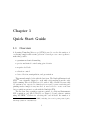
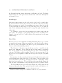
The modern data acquisition system consists of a National Instruments
PCI acquisition card (the PCI-6111, see Figure 1.1) and software written
using LabVIEW.1 Criteria for selecting the card included the number of
1
For more information about LabVIEW, including demos and a getting started guide,
visit http://www.ni.com/labview/.
1
2
CHAPTER 1. QUICK START GUIDE
Figure 1.1: National Instruments PCI-6111 data acquisition card.
digital to analog and analog to digital converters (DAC’s and ADC’s), input
and output voltage ranges, and maximum output rate of the DAC’s.
1.2
Abreviated Procedures
Collecting data using the Instructional Scanning Tunneling Microscope is
done using the following steps. If more information is required, Chapter 2
provides details about each step.
1. prepare a conducting sample (e.g. a gold grating)
2. prepare a tip from tungsten or platinum iridium wire
3. mount sample and tip into vibration isolated STM head
4. set STM panel controls (servo loop response, bias voltage, etc.)
5. load the Burly Control software
6. configure the Burly Control software
7. begin tunneling using the STM panel Tip Approach Controls
8. start the sweep
9. retract tip from sample
1.2. ABREVIATED PROCEDURES
3
10. define and apply a data filter if desired
11. save images
Chapter 3 gives an example and provides the settings to produce the data.
Chapters 5 through 8 discuss aspects of the data manipulation available to
the user, but are not necessary in order to use the STM. An overview of uptdating the Burly Control software and this manual is given in Chapter 4. This
chapter also includes details and specific instructions on particular changes
that may be made.
Chapter 2
How to Scan a Surface
Several steps need to be completed in order to obtain a surface image. There
is a section that corresponds with each one of these steps.
1. prepare a conducting sample (e.g. a gold grating)
2. prepare a tip from tungsten or platinum iridium wire
3. mount sample and tip into vibration isolated STM head
4. set STM panel controls (servo loop response, bias voltage, etc.)
5. load the Burly Control software
6. configure the Burly Control software
7. begin tunneling using the STM panel Tip Approach Controls
8. start the sweep
9. retract tip from sample
10. calibrate scales and return to step 8 (if required)
11. define and apply a data filter if desired
12. save images
This paper will be concerned mainly with using the software, i.e. steps 5,
6, 8, 11, and 12. Section 3 of the Instructional Scanning Tunneling Microscope Workbook provided by Burleigh gives much more detailed information
about the other steps than this manual.
5
6
CHAPTER 2. HOW TO SCAN A SURFACE
Figure 2.1: Special diagonal cutters for making tips.
2.1
Preparing a Sample
When preparing the sample, take special care with those from the Burleigh
sample kit. Parts, services, and samples are no longer provided for this
equipment (hence the need for writing the in-house software). Also, make
sure that there is good conduction between the surface and the sample mount.
If there isn’t, the tip will crash into the sample every time. Both the tip and
sample are damaged when this occurs.
2.2
Preparing a Tip
Use the tungsten wire first and only the platinum iridium when the tungsten
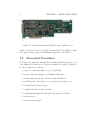
is found to be insufficient.1 After cutting the wire at an angle using the
special diagonal cutters, see Figure 2.1, do not let anything touch it. An
ideal tip will have a single atom on the end. Touching the tip can make it
blunt at the atomic level. When placing the tip into the tip mount, bend the
wire a small amount to hold it in place.
Special diagonal cutters are required because the wire is very hard. Damage to the tool may result when using regular cutters.
1
The platinum iridium wire costs around $100/inch.
2.3. MOUNTING THE TIP AND SAMPLE
7
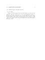
Figure 2.2: Instructional STM front panel.
2.3
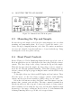
Mounting the Tip and Sample
Because the tip and sample are held in place using magnets, use care when
mounting and unmounting them. It is easy to scratch the surface or to
destroy the tip by bumping them into each other. The surface mount has a
set screw and a handle, but pliers will have to be used with the tip. Using
non-magnetic needle nose pliers can help.
2.4
Front Panel Controls
Refer to Figure 2.2. Under Tunneling Controls in the upper left corner of
the front panel there are two dials that set the bias voltage and the reference
current. The bias voltage is the voltage between the tip and the sample.
When the tip approaches the sample, the bias voltage creates a current between the two through quantum tunneling. When this current reaches the
reference current, the tip stops approaching the surface and the STM is ready
to take data.
To the right of these two dials is an LCD display and four buttons. These
allow the user to see the bias voltage, reference current, actual tunneling
current, and the piezoelectric transducer (PZT) voltage one at a time.
Below the four buttons are three dials that control the Servo Loop Response: time constant, gain, and filter. The time constant determines how
fast the tip will react (move up and down) as the surface is being scanned.
Gain determines by how much the tip reacts and the filter eliminates high
frequencies to discourage oscillations. Read Section 3.5 of the Instructional
Scanning Tunneling Microscope Workbook for typical values.
8
CHAPTER 2. HOW TO SCAN A SURFACE
The Scan/Offset Controls in the middle of the front panel affect the
scanning of the tip. The Magnification knob decreases the distance swept
by the factor selected. Two slides are provided that allow the user to change
the location of the sweep on the surface of the sample.
Understanding how to use the Tip Approach Controls on the right side
of the panel is very important. Incorrect use can lead to damaging the tip
by allowing it to crash into the surface.
There are three tip control buttons. The two white ones provide coarse
control and the red one provides fine control. The coarse control buttons
cause a finely threaded screw to rotate and move a lever to which the tip
is attached. Fine movement is done using the PZT. Take care when using
the coarse adjustments that the tip doesn’t crash into the surface or move
beyond its limits. If the tip assembly is retracted too far, the screw can get
jammed.
The Auto Approach button is used in conjunction with the Coarse Retract
button. To begin tunneling using the auto approach function, tap the Coarse
Retract button and then the red Auto Approach button. While the system
is approaching the surface, the Auto Approach light will flash. When the
tip is close enough to the surface to allow a tunneling current equal to the
reference current, the Auto Approach light is steady and the auto approach
stops. The microscope is now tunneling and ready to take data.
Taping the red button while the microscope is tunneling activates the
fine retract. This retracts the tip from the surface beyond tunneling distance
using the PZT. To return to the tunneling state, tap the red button again.
2.5
Burly Control Main Window
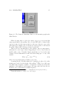
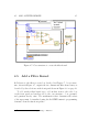
When the the Burly Control software has loaded, you should see a window
similar to Figure 2.3. There are three plots on three different tabs labeled
3D Plot, Surface Data, and Deviation of Data. The surface plot is a
2-dimensional, intensity plot. At each (x, y) grid point, data is taken repeatedly2 . The deviation plot is the standard deviation of this data.
2
The number of points depend on the dwell time – see the discussion about dwell time
on page 12
2.5. BURLY CONTROL MAIN WINDOW
Figure 2.3: The Burly Control main window.
9
10
CHAPTER 2. HOW TO SCAN A SURFACE
Figure 2.4: The Burly Control configuration window.
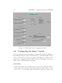
2.6
Configuring the Burly Control
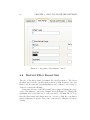
Before performing a sweep of the surface, configure the software by clicking on
the Configure button at the lower left-hand side of the main Burly Control
window. A new window will open and will look like Figure 2.4. There are five
parts of the configuration window: Data Points, Scan Ranges, data mode,
Dwell Time, and Electronics Settings.
Data Points
A square grid with sides of length specified by the user defines the number
of data points. For example, if the user specifies 256, there will be a total
of 256 × 256 = 65, 536 points. Once the system is calibrated, change only
2.6. CONFIGURING THE BURLY CONTROL
11
the Zoom Multiplier button when using a different zoom level. The Burly
Control takes care of the plot scales from the value of the Zoom Multiplier
as discussed below.
Scan Ranges
Maximum scanner ranges set the scale for the plots, but do not affect how
the data is taken. However, the scan ranges do affect how the data is taken.
If the scan ranges are equal to the maximum scan ranges, then the tip will
be swept through its entire range. If the scan range is set to, say, half the
value of the maximum, then the tip will be swept through only half of its
entire range.
To obtain the correct scale, the user must scan a surface with a known
periodicity.3 For example, a gold grating with periodicity of 4, 000Å can be
scanned at zoom level 2× to easily calibrate the system and set the max
scanner range.
Data Mode
There are two modes in which the Scanning Tunneling Microscope can run:
topographic and current. When topographic mode is selected in the software,
the data recorded is the height of the microscope tip. In current mode, the
data recorded is the tunneling current.
The behavior of the microscope in the two modes , controlled by the
Servo Loop Response,4 is very different and it is important to understand
how. In topographic mode, the tip must move up and down following the
contours of the surface while scanning. Therefore, the response time of the
tip (the time constant) must be small and the response level (the gain) must
be large.
In current mode, the current level indicates the height of the surface and
so the tip must stay at the same level. As the scans occurs, the surface gets
closer and farther from the tip, changing the amount of tunneling current
that flows between the two. To keep the tip at the same height during the
scan, the time constant must be large and the gain of the loop must be small.
The Tilt Removal check-box indicates whether the best fit plane should
be removed from the data. This option allows the details on the surface to be
3
4
Be sure to account for the zoom level when calibrating the scale.
Refer to Section 2.4 on page 7 for a discussion on the servo loop response knobs.
12
CHAPTER 2. HOW TO SCAN A SURFACE
seen more clearly when the surface is not level. For more information about
how tilt removal is done, see Section 6.
Dwell Time
Dwell time is the time spent at each data point on the square grid over the
surface. Each data point actually consists of a bunch of data taken at regular
intervals. Therefore, doubling the dwell time doubles the pieces of data taken
and doubles the amount of time per scan. In fact, the data in the 3D Plot
found on the main window5 is actually the average of all the data taken at
each point.
Below the Dwell Time slide bar is the Approximate Sweep Time display.
This number is affected by both the dwell time and the number of data points.
Data is taken every 10µs.
Electronics Settings
The Zoom Multiplier setting in the software affects how the data is presented. The plot ranges are divided by the value of the Zoom Multiplier.
For example, if both the scale range and the maximum scale range for the
x-axis are 4000Å and the Zoom Multiplier is set to 2×, the plot range will
be 2000Å. Therefore, the scan ranges should not be changed when different
zoom levels are selected.
Bias Voltage and Tunneling Current settings are provided for reference only and affect neither how the data is taken nor presented.
2.7
Quantum Tunneling
Once a tip and a sample have been prepared and the software has been
configured, the system can be used to scan the surface. Bring the tip within
tunneling distance by briefly tapping the Course Retract button and then
pushing the Auto Approach button. The LED to the right of the Auto
Approach button should start blinking. When the LED stays steady without
blinking, the system should be tunneling. Check that the tunneling current
5
Refer to Figure 2.3 on page 9.
2.8. SCANNING A SURFACE
13
Figure 2.5: The Burly Control sweep progress bar.
is in the ball park of the reference current by using the Tunneling Controls
buttons.6
2.8
Scanning a Surface
To start scanning the surface, click the Start Sweep button in the lower
left corner of the Burly Control main window. A progress bar will appear
showing the approximate time remaining, see Figure 2.5. The sweep cannot
be stopped once it has begun. Use the Approximate Sweep Time in the
Burly Control configuration window to estimate the duration of the process.
2.9
Retracting the Tip
After the sweep has finished, it is a good idea to retract the tip from the
surface to reduce the possibility of crashing the tip. One may use either the
fine or the course retract. If the Fine Retract button is used, the PZT itself
retracts the needle and therefore the system can be returned to the tunneling
state quickly by tapping the red Fine Retract button again.
2.10
Calibration
As shown in Figure 2.3 on page 9, the surface is shown with a scale (in Å).
In order to calibrate the scale, a sample with a known structure must be
scanned. It is convenient to use a grating with a known period, like the
4000 Å gold grating in the lab.
There are two ways to calibrate the scale: 1) measure the period directly
on the 3D or intensity plot itself or 2) use the Fast Fourier Transform option in
6
See Section 2.4 on page 7 for a discussion of the controls.
14
CHAPTER 2. HOW TO SCAN A SURFACE
the software to measure the period automatically and give a suggestion for the
maximum scale value. In either case, the value of the Max scanner range
in x in the Configuration Window will have to be changed (see Figure 2.4
on page 10).
The Direct Method
The first method is simpler to understand, but requires a calculation and
is less precise. After finishing a sweep of a sample with a known period,
estimate the period shown in either the 3D or the intensity plot. The best
way to do this is to measure the distance spanned by as many periods as
possible and divide that by the number of periods. Why is this superior to
measuring only a single period?
When updating the Max scanner range in x using the first method, be
sure the account for the Scanner range in x and the Zoom Multiplier.
Both of these values affect the scale shown in the graphs, but the Zoom
Multiplier does not change the actual distance swept by STM.
The Fourier Transform Method
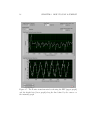
The second method involves using a Fourier transform and picking out the
dominant frequency component – which is done by the software. To use this
method, select the Surface Data tab on the Burly Control Main Window,
position the two cursors on the intensity graph to define a cross section
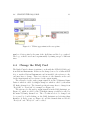
across the grating, and click on the Fourier Transform button shown in
Figure 2.6. A window similar to Figure 2.7 will appear. The lower graph
shows the height of the surface along the line between the cursors. The upper
graph is the Fast Fourier Transform (FFT) of that height data.
Figure 2.7 is actually simulated data:
2π
x + noise
(2.1)
sin
4000
Notice that the frequency component of the 4000 Å period can be seen in
the upper plot. Becuase of the noise and an imperfect choice of the cursor
positions, the measured frequency is about 0.0002523 1/Å, not exactly 1/4000
as expected. This corresponds to a period of 3964 Å and the software suggests
changing the Max sanner range from 32,000 to about 32,300 Å.
2.10. CALIBRATION
15
Figure 2.6: The Fourier Transform button on the intensity graph in the
Main Window.
When choosing where to place the cursors, choose a cross section that
cuts perpendicular to the grating. Also, a better FFT will be obtained if the
cursors are placed at the same position on the wave, that is to say, at the
same phase. For example, place both cursors on wave peaks or both between
the peaks. Why is this best (more advanced question)?
This is all done automatically by the software, but it is important to
understand to some degree what is happening in order to know when an
invalid result occurs. Normally, Fourier transforms are done in the time
domain, but the mathematics is still valid when using space or any other
variable.
Z +∞
f (x)e−i2πkx dx
F (k) =
(2.2)
−∞
where k is a spacial frequency in units of, say, 1/Å.
A grating should look fairly sinusoidal: h0 sin(2πk0 x), where 1/k0 is the
grating period and h0 is the height of the grating.7 What does a sine wave
look like in the frequency domain? A frequency domain plot shows the
amplitude of the signal at each frequency. Because a sine wave has only one
frequency, it is a delta function at that frequency.8
7
8
Spacial frequency is denoted with k to distinguish it from frequency in time, f .
Technically, sin(2πk0 x) → h0 [δ(k − k0 ) − δ(k + k0 )]/2.
16
CHAPTER 2. HOW TO SCAN A SURFACE
Figure 2.7: The Fourier transform window showing the FFT (upper graph)
and the height data (lower graph) along the line defined by the cursors on
the intensity graph.
2.11. FILTERING THE DATA
17
The FFT is an efficient algorithm that computes the discrete Fourier
transform. If sampling is sufficiently high (i.e. there are many data points
between the cursors), this is a good numerical approximation of the Fourier
transform in Equation 2.2.
2.11
Filtering the Data
Filtering data refers to selectively passing some frequency components and
rejecting others. Many signals can be written as a (possibly infinite) sum
of sinusoidal signals, each of a different frequency and amplitude. A lowpass filter, for example, will significantly decrease the amplitude of sinusoids
with high frequencies and leave amplitudes of sinusoids of low frequencies
relatively unchanged.
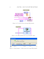
To filter the data, define the type and extent of the filter by clicking on
the Define Filter button in the lower right corner of the Burly Control
main window, see Figure 2.3. In the upper left corner of the filter definition
window, Figure 2.8, one of three types of filters may be chosen: box, pyramid,
or gaussian. The filter kernel, the function used to filter the data, is defined
on a square grid of length specified by the user.
Filtering is done using a method known as convolution.9 Basically, lowpass filtering consists of taking the weighted average of neighboring data
points. The filter kernel gives the weight of each point and the kernel size
determines how many neighbors are included in the average. For example, if
one chooses a 5 × 5 box for the kernel, each data point will be the unweighted
average of the data point and 24 of its neighbors.
2.12
Saving Images to Disk
An image of the filter kernel can be saved to be included with a lab report.
Click the button corresponding to the images you would like to save, select
the type of image in the dialog that appears (PNG, JPEG, or BMP), and
click OK. Choose the location and name of the file to save using the default
Windows file saving dialog that pops up as in Figure 2.9.
9
See Chapter 8 to learn about the process used or visit http://www.jhu.edu/
signals/discreteconv2/index.html
to gain an intuition about (1-dimensional) con~
volution through interactive examples.
18
CHAPTER 2. HOW TO SCAN A SURFACE
Figure 2.8: The Burly Control filter definition window.
Figure 2.9: Save image dialog.
Chapter 3
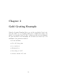
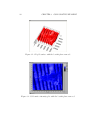
Gold Grating Example
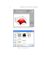
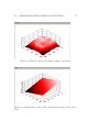
Using the Scanning Tunneling Microscope and the new Burly Control software, the surface of a gold grating with period of 4000Å was scanned. As
usual for topographic scans, the time constant was almost at its minimum,
the gain was almost at its maximum, and the filter was all the way to its
maximum. Scan parameters included:
• 0.1 ms dwell time
• 256 × 256 data points
• 2× zoom factor
• tilt removal on
• bias voltage of 1.31 V
• reference current of 15.3 nA.
19
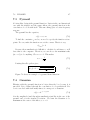
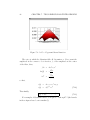
20
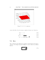
CHAPTER 3. GOLD GRATING EXAMPLE
Figure 3.1: 3D gold surface with the best-fit plane removed.
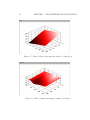
Figure 3.2: Gold surface intensity plot with the best-fit plane removed.
Chapter 4
How to Update the Software
All software has been written using National Instrument’s LabVIEWTM .
LabVIEW1 is a graphical programming environment with many built-in tools
that make interfacing with external instruments easy. The university has a
site license for the professional version of LabVIEW, which is required to
make a standalone application.
4.1
Basic Editing Information
The Burly Control source code is located in a directory called “Burly Control” and it’s subdirectories. Open Burly Control.vi and view the block
diagram. Several variables are initialized here, but the functionality is within
the while loop. Inside the while loop, an event structure handles the commands from the user.
The event structure inside the while loop has a case for each of the eight
buttons available to the user: Configure, Start Sweep, Define Filter,
Apply Filter, Save 3D Image, Save Intensity Image, Save 3D Std Dev
Image, Quit.
The configure button merely calls Configuration.vi which opens the
configuration dialog. The Start Sweep button calls four custom VI’s, one
of which is Single Sweep.vi. Single Sweep.vi performs the actual data
acquisition and returns the data arrays.
There are about 20 custom VI’s. Icons for these cutsom VI’s are all blue
in order to pick them out easily, an example is shown in Figure 4.1.
1
http://www.ni.com/labview/
21
22
CHAPTER 4. HOW TO UPDATE THE SOFTWARE
Figure 4.1: Custom VI’s all have blue icons with a descriptive name written
in black, like Scale Data and Disp Data shown here.
Figure 4.2: Setting the sampling frequency in Hz.
4.2
Change the Data Acquisition Frequency
The data acquisition frequency is a global variable found in Global Config
Params.vi. However, the variable’s value is set in the main VI, Burly
Control.vi. The value is set as shown in Figure 4.2. Be aware that the
sampling frequency is limited by the DAQ card used. If the DAQ card needs
to be changed, see Section 4.4.
4.3
Change the Sweep Time Estimate
If the Burly Control system changes computers (or if Windows starts to run
very slowly for some reason), it may be necessary to adjust the estimated
sweep time. The sweep time is displayed for the user in the Configuration
window;2 but the estimate is done by the Sweep Time VI. The code to calculate the estimate is in Figure 4.3.
Most likely, only the Loop overhead in ms, shown in the figure as the
value 2.3, would need to be changed. The function simply multiplies the
2
The Configuration Window is shown in Figure 2.4 on page 10
4.4. CHANGE THE DAQ CARD
23
Figure 4.3: VI that approximates the sweep time.
number of data points by the sum of the dwell time and the loop overhead.
The loop overhead was found experimentally by timing sweeps of different
sizes.
4.4
Change the DAQ Card
The Burly Control software is written to work with the PCI-6111 DAQ card
from National Instruments. If this card is changed, moved to a different PCI
slot, or another National Instruments card in installed, the reference to the
card may have to change. There is a reference to the channels on the card
for the input signals and a reference for the output signals.
The reference for the analog input signals is in the VI Create Input
Task.vi which is called by Single Sweep.vi which is called by the main
VI, Burly Control.vi. The channel specification may have to change from
“Dev1/ai0” to “Dev2/ai0” for example, see Figure 4.4.
The reference for the analog output signals is in the DAQ Assistant, see
Figure 4.5, which is called by the VI Single Sweep.vi which is called by
the main VI, Burly Control.vi. The code that needs to be changed can
be accessed by double-clicking on the DAQ Assistant and selecting Show
Details. A dialog opens, see Figure 4.6, and the channels that are labeled
“Dev1/ao0” and “Dev1/ao1” can be edited.
24
CHAPTER 4. HOW TO UPDATE THE SOFTWARE
Figure 4.4: Code that references the input DAQ channels.
Figure 4.5: The DAQ Assistant used for producing the output.
Figure 4.6: DAQ Assistant code that references the output DAQ channels.
4.5. ADD A FILTER KERNEL
25
Figure 4.7: Case structure to create the filter kernel.
4.5
Add a Filter Kernel
In Filter.vi, the filter is created as described in Chapter 7. A case structure, shown in Figure 4.7, outputs the two-dimensional filter kernel array as
described by the selections on the front panel shown in Figure 2.8 on page 18.
To add another filter kernel type, add another item to the radio box
on the front panel and another case to the case structure – box, pyramid,
and gaussian already exist. The mathematics that determines the values
of the array must be translated using the LabVIEW numeric programming
elements3 from the functions palette.
3
Functions Palette → Programming → Numeric
26
CHAPTER 4. HOW TO UPDATE THE SOFTWARE
Figure 4.8: Properties of the numeric control.
4.6
Restrict Filter Kernel Size
The size of the filter kernel determines the cutoff frequency. The larger
the filter, the lower the cutoff frequency, the more high frequency data gets
filtered out. Because this data manipulation can be taken too far, it may be
desired to restrict the filtering.
Restricting the size of the filter kernel only requires adjusting the properties of the numeric control Key Length, shown in Figure 4.8. Change the
maximum value of the filter size to some reasonable, odd limit, like 11. Note
that the filter kernel will always have an odd size so that the convolution
sum is symmetric about the data point of interest (see Chapter 8 for more
details).
4.7. UPDATING THIS MANUAL
4.7
27
Updating this Manual
This manual is written in LATEX4 and consists of several parts. Various
chapters were written independently. This allows them to be printed by
themselves as complete documents and easily included in other documents,
including this manual. Chapters that have been included separately are
Chapter 3 Gold Grating Example, Chapter 6 Plane Removal, Chapter 7 TwoDimensional Filter Kernels, and Chapter 8 Two-Dimensional Convolution.
LATEX documents are created using text files, usually with the extension
.tex. The chapters that have been written separately are found in subdirectories. There is a LATEX file and a .body file for each of these chapters. All
of the content of each chapter is written in the .body file and included in the
LATEX file, which contains information about the title, document type, etc.
This is how the content is included in several documents.
For example, if the content of the chapter on the Plane Removal needs to
be updated, go to the plane-removal directory and edit the plane-removal.body
file. Then execute pdfLatex, or simply run make in that directory. A make
file is provided in each directory.
4 A
LT
EX is a high-quality typesetting environment available for Unix/Linux, MacOS X,
and Microsoft Windows and is used extensively for scientific and mathematical documents.
Learn more at http://www.latex-project.org/ or read lshort.pdf, the excellent tutorial
found at http://www.ctan.org/tex-archive/info/lshort/english/.
Chapter 5
Fourier Transform of Height
Data
5.1
Introduction
Displaying the Fourier transform of the surface data for an arbitrary section
through the data is not a trival process because few, if any, of the data points
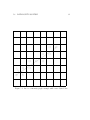
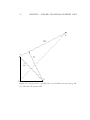
will lay on the line chosen by the user. For example, Figure 5.1 shows a grid
of 8 × 8 surface measurements. The user has chosen a line by placing cursors
at locations (Row, Column) = (7, 1) and (3, 7) and a line has been drawn
between these points. In this example, only one data point, the one at (5, 4),
lays exactly on the line.
Several step are involved in finding the frequency content along the userdefined line. First, data points to include on the line need to be chosen
(Section 5.2). Second, the value of the data and it’s position along the line
need to be found (Section 5.3). Third, the unevenly spaced data along the
line will have to be resampled evenly for the transform (Section 5.4). Finally,
a Fourier transform needs to be calculated.
It is assumed in this analysis that the resolution of the surface data is
large compared to the length of the line. Another way to say this is the
spacing between the data is small compared to the length of the line. This
means that height of the surface over the line can be approximated by the
nearby data. If this assumption were false, one would have to go to a secondorder approximation by looking at the divergence of the surface around the
line. Also, this means that a linear approximation (or even a “zero-order
29
30
CHAPTER 5. FOURIER TRANSFORM OF HEIGHT DATA
hold”) will be sufficient when resampling the data in Section 5.4.
5.2
Data Point Selection
Data is selected based on how close it is to the line. Three examples of these
distances are shown in Figure 5.1. To find the minimum distance from a data
point to the line, vectors are defined, as shown in Figure 5.2, from the origin
O to the ends of the user-defined line, A and B, and to the data point in
question, C.
To determine whether
a data point is included in the line, the length of
→
→
−
−
vector D , D ≡ D , will be required.
−→
D = AC sin(∠BAC)
and since,
and sin(θ) =
−→ −→
AB · AC
cos(∠BAC) = −→ −→
AB AC p
cos2 (θ) − 1,
v
u −→ −→ 2
−→ u
u AB · AC
D = AC t −→ −→ − 1
AB AC 5.3
(5.1)
Data Point Location
The position of the data point along the user-chosen line will be where the
point’s perpendicular bisector intersects the line. Therefore, the position can
be determined in a very similar manner to finding the distance from the line
in Section 5.2. Referring to Figure 5.2,
−→ −→
−→
AB · AC
l = AC cos(∠BAC) = −→
(5.2)
AB 5.3. DATA POINT LOCATION
31
r
m
m
m m
m
m
m
m
m J
J
J
J
J
J
J
J
r
J
m
Jm
Figure 5.1: An 8 × 8 intensity graph example with a user defined line.
32
CHAPTER 5. FOURIER TRANSFORM OF HEIGHT DATA
s
*
B
−→
AB O
A
K
A A
A −
→
s A D
6
@
A
@
A
@
A
@
A
−→@
A
AC @
A
@
A
@
A
@
A
@
A
@
@ A
@ A
@ A
@A C
R
@
-As
Figure 5.2: Vectors used to calculate the closest distance from a data point,
C to the user chosen line AB.
5.4. RESAMPLING THE DATA
33
Item Description
N
Number of data points along the line
−→
Length of line = AB l
hu [i]
Unevenly spaced height of surface
he [i]
Evenly spaced height of surface
xu [i]
Unevenly spaced locations of the data along the line
xe [i]
Evenly spaced locations of the data along the line
Table 5.1: Variable definitions
5.4
Resampling the Data
Because most of the data isn’t exactly on the line, the data is not evenly
spaced along the line and this is a problem when calculating the Fourier
transform. As stated in the introduction, it is assumed the surface resolution
is great enough to use linear interpolation between the unevely spaced data
points.
Refer to the variable definitions described in Table 5.1. The spacing
bewteen points in he [i] should end up being l/(N − 1) and therefore the
evenly spaced data point locations are xe [i] = il/(N − 1).
Now the height of the surface must be approximated at each xe [k] location. The idea is to do a linear interpolation between the hu [m] and hu [m+1]
values, where m is the largest index such that xu [m] ≤ xe [k]. Then the approximate height at location xe [k] is
he [k] = hu [m] + ∆h = hu [m] + (slope) (∆x)
he [k] = hu [m] + (hu [m + 1] − hu [m]) (xe [k] − xu [m])
(5.3)
Chapter 6
Plane Removal
6.1
Derivation
This paper provides the derivation of the equations used to remove the bestfit plane from a set of N data points (xi , yi , zi ). It is adapted to the special
case that the data collected consists of measurements made over a rectangular
grid of dimensions (m, n). The best-fit plane is found using the least-squares
method.
The equation of a plane is
ax + by + z = c
(6.1)
z(x, y; a, b, c) = c − ax − by
(6.2)
or
We want to minimize (with respect to the parameters a, b, and c) the
sum of the squares of the vertical distances between the data and the plane,
call this ∆.
∆(xi , yi ; a, b, c) =
N
X
[zi − z(xi , yi ; a, b, c)]2
i=1
35
(6.3)
36
CHAPTER 6. PLANE REMOVAL
Extrema occur where the derivatives are zero, so,
N
X
∂∆
= 2
[zi + axi + byi − c] xi = 0
∂a
i=1
(6.4)
N
X
∂∆
= 2
[zi + axi + byi − c] yi = 0
∂b
i=1
(6.5)
N
X
∂∆
= −2
[zi + axi + byi − c] = 0
∂c
i=1
(6.6)
Equation 6.6 gives,
c=
N
1 X
[zi + axi + byi ]
N i=1
(6.7)
Which simply states that the plane cuts through the “center of mass” of the
data: zave = c − axave − byave .
Put Equation 6.7 into Equation 6.4,
#
"
X
X
1
(zj + axj + byj ) xi = 0
(6.8)
zi + axi + byi −
N j
i
Splitting up the sums,
X
X
X
zi xi + a
x2i + b
xi yi −
i
i
i
1 XX
a XX
b XX
zj xi −
xi xj −
yj xi = 0
N i j
N i j
N i j
(6.9)
and collecting terms,
"
a
#
XX
1
x2i −
xi xj
N i j
i
"
#
X
1 XX
−b
xi yi −
yj xi
N
i
i
j
X
1 XX
+
zi xi −
zj xi = 0
N
i
i
j
X
(6.10)
6.1. DERIVATION
37
It is convenient to define an operator for shorthand,
?(u, v) ≡
N
X
i=1
ui u j −
N
N
1 XX
uj v j
N i=1 j=1
(6.11)
Note also that ?(u, v) = ?(v, u).
Then we have,
−b ?(x, y) − ?(x, z)
(6.12)
a=
?(x, x)
To find b, use Equations 6.7 and 6.12 in Equation 6.5,
X
b ?(x, y) + ?(x, z)
zi −
xi + byi yi
?(x,
x)
i
(
)
X 1 X
b ?(x, y) + ?(x, z)
−
xj + byj
= 0 (6.13)
zi −
N
?(x,
x)
i
j
Separating the sum and collecting terms,
X
?(x, z) X
1 XX
za yi −
xi yi −
yi zj
?(x, x) i
N i j
i
1 ?(x, z) X X
xj yi
N ?(x, x) i j
)
(
1 ?(x, y) X X
?(x, y) X
xi yi +
yi xj
+b −
?(x, x) i
N ?(x, x) i j
(
)
X
XX
1
+b
yi2 −
yi yj = 0
N i j
i
+
(6.14)
Then using the definition of the ? operator from Equation 6.11,
b=
?(x, y) ?(x, z) − ?(x, x) ?(y, z)
?(y, y) ?(x, x) − ?2 (x, y)
(6.15)
Now all of the parameters that define the plane have been found. However, when the data is measured
PNover a rectangular grid as stated earlier, the
sums cannot be performed as i=1 . The set of data is kept in three vectors,
one of length m, one of length n, and one of dimensions (m, n). Computing
these sums will take a bit more work.
38
CHAPTER 6. PLANE REMOVAL
6.2
Computing the Sums
We will need all six combinations of the ? operator acting on x, y, and z
except ?(z, z). Because I have a grid of data of dimensions m × n, I need to
translate these sums over the N points into sums over my data vectors. I have
two 1-dimensional vectors representing the position on the surface, call them
x̂i and ŷj (or x̂(i) and ŷ(j)), and a 2-dimensional vector that represents the
height above the surface, call it ẑ(i, j), where i ∈ [0, m − 1] and j ∈ [0, n − 1].
Equation 6.16 shows the N data elements of the grid and Equation 6.17
shows the values of the 2-dimensional array, ẑ, in a similar fashion.
data =
=
z1
z2
zm+1
..
.
zm+2
..
.
···
···
zm
z2m
..
.
znm−m+1 znm−m+2 · · · znm
ẑ(0, 0)
ẑ(0, 1)
..
.
···
···
ẑ(1, 0)
ẑ(1, 1)
..
.
ẑ(m − 1, 0)
ẑ(m − 1, 1)
..
.
ẑ(0, n − 1) ẑ(1, n − 1) · · · ẑ(m − 1, n − 1)
(6.16)
(6.17)
Using this comparison between the two ways to represent the data, we
may now rewrite the sums over the elements of the data vectors so that these
sums can be implemented using a computer.
Because the x-data (y-data) has m (n) terms, we can sum over those
terms and multiply by n (m). Notice the difference between the vector x and
the vector x̂. The former has N elements, one for each measurement, and
the latter has m values, one for each column of the rectangular grid.
N
X
i=1
N
X
i=1
xki
= n
m−1
X
yik = m
x̂ki
i=0
n−1
X
ŷik
(6.18)
(6.19)
i=0
When there is a double sum, the cross terms are included because the
6.2. COMPUTING THE SUMS
39
sums can be separated. Therefore,
"
N X
N
X
xi xj =
n
m−1
X
i=1 j=1
#2
(6.20)
x̂i
i=0
"
N X
N
X
yi yj =
m
i=1 j=1
N X
N
X
n−1
X
#2
(6.21)
ŷi
i=0
xi yj = mn
"m−1
X
i=1 j=1
x̂i
# " n−1
X
i=0
#
(6.22)
ŷj
j=0
Looking at Equation 6.17, we can see that
N
X
xi yi = x̂0 ŷ0 + x̂1 ŷ0 + x̂2 ŷ0 + · · · + x̂m−1 ŷ0 +
i=1
x̂0 ŷ1 + x̂1 ŷ1 + x̂2 ŷ1 + · · · + x̂m−1 ŷ1 +
..
.
x̂0 ŷn−1 + x̂1 ŷn−1 + · · · + x̂m−1 ŷn−1
so
N
X
i=1
xi yi =
m−1
n−1
XX
x̂i ŷj =
i=0 j=0
"m−1
X
x̂i
# " n−1
X
i=0
(6.23)
#
ŷj
(6.24)
j=0
Similarly when we have a single sum with z in the equation,
N
X
xi zi = x̂0 ẑ00 + x̂1 ẑ10 + x̂2 ẑ20 + · · · + x̂m−1 ẑm−1,0 +
i=1
x̂0 ẑ01 + x̂1 ẑ11 + x̂2 ẑ21 + · · · + x̂m−1 ẑm−1,1 +
..
.
x̂0 ẑ0,n−1 + x̂1 ẑ1,n−1 + · · · + x̂m−1 ẑm−1,n−1
(6.25)
and this is equivalent to two sums:
N
X
xi zi =
i=1
N
X
i=1
m−1
n−1
XX
x̂i ẑij
(6.26)
ŷj ẑij
(6.27)
i=0 j=0
yi zi =
m−1
n−1
XX
i=0 j=0
40
CHAPTER 6. PLANE REMOVAL
The only thing that remains is a double sum over z and x or y. This
simply splits up into two parts as before, one over i for x̂i or ŷi and the other
a double sum over i and j for ẑij .
N X
N
X
"
xi zj =
n
m−1
X
i=1 j=1
N X
N
X
x̂i
# "m−1 n−1
XX
i=0
"
yi zj =
i=1 j=1
m
#
(6.28)
ẑij
i=0 j=0
n−1
X
i=0
ŷi
# "m−1 n−1
XX
#
ẑij
(6.29)
i=0 j=0
Notice that in the special case of an m × n grid of points, ?(x, y) = 0.
N
N
1 XX
xj yj
N
i=1
i=1 j=1
"m−1 # " n−1 #
"m−1 # " n−1 #
X
X
X
mn X
x̂i
ŷi
=
x̂i
ŷi −
mn i=0
i=0
i=0
i=0
?(x, y) =
N
X
xi yj −
= 0
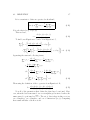
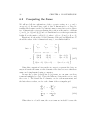
6.3
(6.30)
Summary
Removing the best-fit plane found by the method of least squares involves
a number of sums over the three dimensions of data values. In this paper,
the data is assumed to be the third dimension measured over a rectangular
grid of dimensions (m, n). Therefore, the x-data vector (x̂) has length m,
the y-data vector (ŷ) has length n, and the z-data vector (ẑ) has dimensions
(m, n).
6.3.1
Equations
Because the sums often appear in the same form, it is convenient to define a new operator for any two vectors u and v. This definition, given in
Equation 6.11, is repeated here for convenience.
?(u, v) ≡
N
X
i=1
ui u j −
N
N
1 XX
uj v j
N i=1 j=1
6.3. SUMMARY
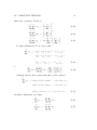
41
Table 6.1 shows the different sums that are needed for the various ?
operations. Table 6.2 summarizes the calculation of the necessary sums using
the data vector values. The necessary ? operations are as follows,
?(x, x) =
?(y, y) =
?(x, z) =
?(y, z) =
"m−1 #2
X
n
x̂i
n
x̂2i −
m
i=0
i=0
" n−1 #2
n−1
X
m X
m
ŷi2 −
ŷi
n i=0
i=0
"m−1 # "m−1 n−1 #
m−1
n−1
XX
XX
1 X
x̂i ẑij −
x̂i
ẑij
m i=0
i=0 j=0
i=0 j=0
" n−1 # "m−1 n−1 #
m−1
n−1
XX
XX
1 X
ŷj ẑij −
ŷi
ẑij
n
i=0 j=0
i=0
i=0 j=0
m−1
X
(6.31)
(6.32)
(6.33)
(6.34)
Using Equations 6.7, 6.12, and 6.15 with Equation 6.30, we have,
?(x, z)
?(x, x)
?(y, z)
b = −
?(y, y)
c = zave + axave + byave
a = −
6.3.2
(6.35)
(6.36)
(6.37)
Computational Steps
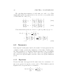
The steps that should be taken are:
1. Calculate the last 7 sums in Table 6.1.
2. Use those sums to calculate the necessary values of the ? operator
(Equations 6.31 - 6.34).
3. Obtain the parameters of the plane using Equations 6.35 - 6.37.
4. Subtract the height of the best-fit plane from each of the z-data values.
42
CHAPTER 6. PLANE REMOVAL
?(x, x) ?(y, y) ?(x, y) ?(x, z) ?(y, z)
PN
x2i
PN
yi2
i=1
i=1
×
×
PN
xi yi
PN
xi zi
PN
yi zi
i=1
i=1
i=1
×
×
×
PN PN
xi xj
PN PN
yi yj
PN PN
xi yj
PN PN
xi zj
PN PN
yi zj
i=1
i=1
i=1
i=1
i=1
j=1
j=1
j=1
j=1
j=1
Pm−1
x̂i
Pn−1
i=1
ŷi
Pm−1
x̂2i
Pn−1
ŷi2
i=0
i=1
i=1
Pm−1 Pn−1
i=1
×
√
√
√
√
√
ŷj ẑij
i=1
×
√
Pm−1 Pn−1
i=1
×
√
x̂i ẑij
i=1
×
√
Pm−1 Pn−1
i=1
×
i=1
ẑij
√
√
√
√
Table 6.1: Sums required for the √
various ? operations. Sums over the N data
points are marked with ×’s and ’s are used for sums over the data vectors.
6.3. SUMMARY
Sum Over Data
PN 2
i=1 xi
PN 2
i=1 yi
PN
i=1 xi yi
PN
i=1 xi zi
PN
i=1 yi zi
PN PN
i=1
j=1 xi xj
PN PN
j=1 yi yj
i=1
PN PN
j=1 xi yj
i=1
PN PN
j=1 xi zj
i=1
PN PN
j=1 yi zj
i=1
43
Sum Over Vector Values
P
2
n m−1
i=0 x̂i
P
2
m n−1
i=0 ŷi
i
i hP
hP
n−1
m−1
j=0 ŷj
i=0 x̂i
Pm−1 Pn−1
i=0
j=0 x̂i ẑij
Pm−1 Pn−1
i=0
j=0 ŷj ẑij
Pm−1 2
n i=0 x̂i
Pn−1 2
m i=0 ŷi
i
i hP
hP
n−1
m−1
ŷ
x̂
mn
i
j=0 j
i=0
Pm−1 hPm−1 Pn−1 i
n i=0 x̂i
j=0 ẑij
i=0
h
Pn−1 Pm−1 Pn−1 i
m i=0 ŷi
j=0 ẑij
i=0
Equation Page
6.18
38
6.19
38
6.24
39
6.26
39
6.27
39
6.20
39
6.21
39
6.22
39
6.28
40
6.29
40
Table 6.2: Sums taken over all data values from 1 to N and the corresponding
sums taken over the data vectors.
Chapter 7
Two-Dimensional Filter
Kernels
7.1
Introduction
Reducing the amount of high frequency noise in an image can be done with
a two-dimensional low-pass filter. Though filtering improves how the data
appears, be aware that filters can be over used which may hide important
features in the data. The derivation of the filters used by the scanning
tunneling microscope software is given here.
In general, filters should be normalized, i.e. the sum over all the elements
is 1. For all but the most simple filters, normalization is most easily accomplished by letting the computer produce the sum of all the filter elements
and then simply dividing each element by this sum. Therefore, the equations
given here are not necessarily normalized.
For the most part, the notation used in this paper is straight forward, but
it’s rather important to keep the definitions straight. N is the number of filter
elements in the x- and y-directions and n is defined such that N = 2n + 1.
Elements in the filter are be labeled by (i, j) for i, j ∈ [0, 1, 2, . . . , 2n]. The
value of the filter is denoted as z which may be written as z(i, j), z(x, y), or
z(r, φ).
Symmetric filters implies that the center of the coordinate system is the
45
46
CHAPTER 7. TWO-DIMENSIONAL FILTER KERNELS
Figure 7.1: A 5 × 5 box function.
center of the filter. Also, the arrays are numbered from 0, not 1, therefore,
x(i) = i − n
y(j) = j − n
p
r(x, y) =
x2 + y 2
√
rmax ≡ r(x(0), y(0)) = 2n
7.2
(7.1)
(7.2)
(7.3)
(7.4)
Box
The box function is the simplest low pass filter, but it has the most frequency
distortion. An example is plotted in Figure 7.1 and is defined as a uniform
function:
z(i, j) =
1
N2
(7.5)
7.3. PYRAMID
7.3
47
Pyramid
A better filter design is the pyramid function. Just as in the one-dimensional
case with the triangle and the square filters, the pyramid function is the
convolution of a box with itself. This smoothing gives a better frequency
response.
The pyramid has the equation,
z(r) = z0 + mr
(7.6)
To find the constants z0 and m, we need to specify the function at two
points. For one, make the function zero at the corners. That is to say,
z(rmax ) = 0
Because the normalization is difficult to calculate for arbitrary n, we’ll
leave that to the computer. Therefore, we can choose the maximum value
(at r = 0) to be anything. Choose z0 = 1. This makes
1
m = −√
2n
(7.7)
Putting this all together gives,
p
z(i, j) = 1 −
(i − n)2 + (j − n)2
√
2n
(7.8)
Figure 7.2 shows an example of a pyramid kernel function.
7.4
Gaussian
Filtering with the pyramid function is better than the box because it is
smoother. It is obtained through the convolution of a box with itself. If a
box is convolved with itself many times, it converges to a Gaussian.
z(r) = Ae−(r−r0 )
2 /2σ 2
(7.9)
A is the amplitude found through normalization just like in the case of the
pyramid and σ is the standard deviation. We want the Gaussian to be
maximum at the center of the filter, so r0 = 0.
48
CHAPTER 7. TWO-DIMENSIONAL FILTER KERNELS
Figure 7.2: A 15 × 15 pyramid kernel function.
The rate at which the Gaussian falls off determines σ. If we want the
amplitude at the corners to be a fraction, f , of the amplitude at the center
of the filter, then,
2
f A = Aermax /2σ
r2
ln(f ) = − max
2σ 2
2
rmax
2σ 2 =
ln(1/f )
2
so that,
z(r) = Ae−(r/rmax )
z(r) = Af (r/rmax )
2
ln(1/f )
2
(7.10)
Then finally,
z(r) = Af [(i−n)
2 +(j−n2 )
]/2n2
(7.11)
For examples of Gaussian kernels, see Figures 7.3 through 7.5 (the kernels
in these figures have been normalized).
7.4. GAUSSIAN
49
Figure 7.3: A 5 × 5 Gaussian kernel function that falls of to 0.45 of its
maximum value.
Figure 7.4: A 15 × 15 Gaussian kernel function that falls of to 0.9 of its
maximum value.
50
CHAPTER 7. TWO-DIMENSIONAL FILTER KERNELS
Figure 7.5: A 15 × 15 Gaussian kernel function that falls of to 0.003 of its
maximum value.
Chapter 8
Two-Dimensional Convolution
8.1
The Convolution Equation
Because the regular definition of a convolution assumes the data is zero beyond the limits of the array, filtering produces data abnormally close to zero
along the edges of the array. The convolution routine to be employed should
stop at the edges of the data array and use a renormalized kernel.
A two-dimensional convolution is defined as
(x ∗ y)[i, j] ≡
∞
∞
X
X
x[k, l]y[i − k, j − l]
(8.1)
k=−∞ l=−∞
The variable x will be used as the filter kernel and y as the data to be filtered.
If the kernel has size N × N and N = 2n + 1, with n ∈ [0, 1, 2, . . . ], then
the limits of the sum can be reduced. To make the sums consistent with
0-indexed arrays in computer programs, the sums will go from 0 to N − 1.
To keep the kernel centered on the point of evaluation, (i, j), k and l in
Equation 8.1 must be replaced with k − n and l − n, respectively. Therefore,
we have
(x ∗ y)[i, j] =
N
−1 N
−1
X
X
x[k, l]y[i − (k − n), j − (l − n)]
(8.2)
k=0 l=0
Equation 8.2 will work perfectly fine except at the edges where the kernel
“overhangs” the data. Not only will the limits of the sum need to be further
reduced, but the result will have to be renormalized. The sum over all the
51
52
CHAPTER 8. TWO-DIMENSIONAL CONVOLUTION
filter kernel elements is 1, but near the edges when only part of the kernel is
used, it will be necessary to divide by the sum over only those elements that
are used.
8.2
Limits Near the Edges
We need to adjust the upper and lower limits on the sum over k (x-values
or columns) and l (y-values or rows). Normally the sums will be performed
exactly as in Equation 8.2. However, when the point of evaluation, (i, j), is
within n points of the edge of the data, we need to raise a lower limit or
lower an upper limit.
The lower limit for k needs to be adjusted when the point (i, j) is within
n points of the left-hand side (LHS), or when i < n, since there are 2n + 1
points in the filter kernel and the arrays are indexed from 0. Therefore, the
lower limit needs to be
LHS limit = max{0, n − i}
(8.3)
An adjustment is also needed when we are evaluating a point within n
points of the right-hand side (RHS). The index of the last column in the data
is M − 1, so at any point, we are M − 1 − i points from the edge.
RHS limit = 2n − max{0, n − M + 1 + i)}
(8.4)
The top and bottom sides (TS and BS) are very similar since both the
data matrix and the filter matrix are square.
8.3
TS limit = max{0, n − j}
(8.5)
BS limit = 2n − max{0, n − M + 1 + j)}
(8.6)
Normalization
We want to find the subarray that will be used in the convolution. When
the output is being calculated for a point near the edge of the data array,
there may be parts of the kernel we don’t use. The subarray will be defined
by the a start index and a length.
8.4. COMPARISON WITH A SIMPLE CONVOLUTION
53
There are columns on the LHS of the kernel that have to be ignored
whenever i < n. Therefore, when positive, the number of columns on the
LHS that have to be ignored is n − i. So, the column index is
ic = max{0, n − i}
(8.7)
As stated for Equation 8.4, there are M − 1 − i points from the RHS, so we
need to subtract off n − M + 1 − i whenever it’s positive. Therefore, the
number of columns is
lc = [kernel length] − [overlaps on LHS] − [overlaps on RHS]
lc = [2n + 1] − [max{0, n − i}] − [max{0, n − M + 1 + i}]
(8.8)
Similarly for the rows,
ir = max{0, n − j}
(8.9)
lr = [kernel length] − [overlaps on TS] − [overlaps on BS]
lr = [2n + 1] − [max{0, n − j}] − [max{0, n − M + 1 + j}]
(8.10)
In order to normalize, simply divide by the sum of the components in the
subarray defined above.
8.4
Comparison with a Simple Convolution
The original issue addressed by this paper was the large deviations produced
by convolution near the edges of the data. Again, this occurs because the
convolution process assumes the data to be zero in the arrays beyond the
measurements. Using the filtering method of this paper, this artificial deviation can be avoided.
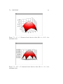
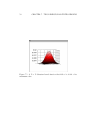
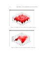
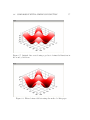
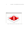
Figure 8.1 shows a 21 × 21 plot of data produced using a random number
generator. Filtering using a 5 × 5 Gaussian kernel is essentially sending the
data through a low-pass filter. The lack of high frequency content in the
filtered data can be seen in both Figures 8.2 and 8.3. However, Figure 8.3
shows that using a conventional convolution, the data is drawn toward zero
at the edges. The filtering process described in this paper, and used to create
Figure 8.2, does not warp the data in this manner.
The same filtering methods were used for a planar and a sinusoidal set of
data. See Figures 8.4 through 8.9.
54
CHAPTER 8. TWO-DIMENSIONAL CONVOLUTION
Figure 8.1: Original data created using a random number generator.
Figure 8.2: Filtered random data using the method of this paper.
8.4. COMPARISON WITH A SIMPLE CONVOLUTION
55
Figure 8.3: Filtered random data using a simple convolution.
Figure 8.4: Original data created with constant slopes in the x and y directions.
56
CHAPTER 8. TWO-DIMENSIONAL CONVOLUTION
Figure 8.5: Filtered planar data using the method of this paper.
Figure 8.6: Filtered planar data using a simple convolution.
8.4. COMPARISON WITH A SIMPLE CONVOLUTION
57
Figure 8.7: Original data created using a product of sinusoidal functions in
the x and y directions.
Figure 8.8: Filtered sinusoidal data using the method of this paper.
58
CHAPTER 8. TWO-DIMENSIONAL CONVOLUTION
Figure 8.9: Filtered sinusoidal data using a simple convolution.