Download User`s Manual

PROSA
Version 3.4
User’s Manual
Peter Güntert
Institut für Molekularbiologie und Biophysik
Eidgenössische Technische Hochschule
CH-8093 Zürich
Switzerland
December 1994
1
© 1994 Institut für Molekularbiologie und Biophysik
Eidgenössische Technische Hochschule
CH-8093 Züric h
Switzerland
2
Contents
Introduction 5
Installation 7
Command Interpreter 11
Commands 21
Variables 33
Macros 37
Examples 41
Algorithms 49
References 57
3
4
Introduction
Introduction
The program package PROSA (“Processing algorithms”) allows to perform the processing steps that lead from the time-domain data furnished by the NMR spectrometer
to the multi-dimensional spectrum. Its functions include linear prediction, apodization, Fourier transformation, automatic phase correction, baseline correction, and formatting of the output for easy use with spectrum analysis programs.
The design of the program is simple both because it does not use computer graphics and the complete multi-dimensional data matrix is kept in memory throughout the
processing. Therefore the implementation of the program on a variety of different
computers is straightforward and time-consuming data processing can be executed in
batch mode. The fully processed spectra can then be displayed on a conventional
graphics station. In the present implementation, the output of PROSA is compatible
with the program package XEASY (Bartels et al., 1994; Eccles et al., 1991).
Since PROSA completely avoids disk storage of intermediate results (i.e., at the outset the time-domain data are read into the computer memory and only the fully processed frequency-domain data are written back onto disk), the computer memory
must be sufficiently large to hold the complete data set. On vectorizing computers the
program achieves high efficiency because of the complete vectorization of all time-consuming routines, which is facilitated by the fact that identical operations are applied
independently to all 1D cross-sections of a data set. PROSA is written in standard FORTRAN-77 and was implemented on a variety of computers.
A description of the program PROSA is given in the following publication:
Güntert, P., Dötsch, V., Wider, G. & Wüthric h K. (1992). Processing of multi-dimensional NMR data with the new software PROSA. J. Biomol. NMR, 2, 619–
629.
In this manual literal input is printed in bold, other input is printed in italics. Optional input is given in square brackets [. . .], and optional input that may be repeated
zero or more times is given in curly braces {. . .}. In examples, output from the program
PROSA is printed in typewriter font.
5
Introduction
Comments, suggestions, and reports on bugs are welcome. Please send them to:
Peter Güntert
Institut für Molekularbiologie und Biophysik, HPM G21
Eidgenössische Technische Hochschule
CH-8093 Züric h
Switzerland
electronic mail: [email protected]
___________________________
6
Installation
Installation
Configuration
The program PROSA is delivered either on tape cartridge as a UNIX “tar”-archive
or via electronic mail as a uuencoded, compressed, tar-archive file . To extract the individual files from the tape cartridge , use the UNIX command:
tar xvf tape-device
[1]
which creates in the current directory a subdirectory called prosa-3.4 that contains
the prototype makefile Makefile.def, the installation help file README, the configuration shell script configure, and the subdirectories help, macro, and src for help
files , macro files , and source files , respectively.
To extract the individual files from the electronic mail file , use the following sequence of UNIX commands:
uudecode mail-file
uncompress prosa-3.4.tar.Z
tar xvf prosa-3.4.tar
[2]
The Makefile is created from the prototype makefile Makefile.def by the shell
script configure using the UNIX command
./configure [system]
[3]
that recognizes the following UNIX computer systems: convex, hp, ibm, nec, sgi,
sun, and generic. If no system is specified, the script tries to determine the correct
system type using the uname command or the HOSTTYPE environment variable.
The script configure assumes that the name of the directory where the program PROSA resides is of the form prosa-version. The system-dependent parameters set by the
configuration script are shown when the script is executed. The following example is
from a Sun-4 computer where the program resides in the directory /home/guentert/
prosa-3.4:
7
Installation
Configuration:
System type
:
Program
:
Makeprogram
:
Version
:
Macro extension :
Base directory
:
RECL unit
:
Time routine
:
Integer length
:
Complex data type:
Precompiler
:
Fortran compiler :
Compiler options :
Linker options
:
Libraries
:
Sun
prosa
makeprosa
3.4
.pro
/home/guentert/prosa-3.4
4 per word
etime(tarray)
1 per real
complex
/lib/cpp
f77
-c -O
RECL unit denotes the record length unit (in units per word) used in record length
specifications in FORTRAN-77 OPEN statements for direct access files .1 The present
version of the program PROSA assumes a word length of 32 bit. On computers with
variable word length, for example the NEC SX-3, it is essential to choose the correct
word length of 32 bit.
Compilation
The executable program prosa, the script makeprosa, the links for help files , and
the default initialization macro init are created by
make
[4]
By default, a standard memory and workspace size will be used. This, and several
other parameters may be changed on the make command line (see the Makefile for
further details). For example:
make MAXS=memory MAXW=workspace PROG=myprosa
[5]
builds a PROSA executable called myprosa with the given memory and workspace
sizes (in words). The script makeprosa can be used to build additional PROSA executables in other directories. The command
makeprosa memory workspace [executable]
1 According
[6]
to the rules of FORTRAN-77 (Kießling & Lowes, 1987), the record length should be
given in words but some compilers assume that it is specified in bytes .
8
Installation
builds a PROSA executable with the given memory and workspace size (in words) in the
current working directory. The makeprosa command can be used to temporarily create a PROSA executable with optimal memory and workspace usage for the execution
of a particular macro (the minimally required memory and workspace sizes for the execution of a macro can be determined with the standard macro job; see p. 38).
The Makefile , the script makeprosa, and the initialization macro macro/
init.pro are generated from the prototype files Makefile.def , src/makeprosa.def,
and src/init.pro.def, respectively. Permanent changes to these files should be made
in the corresponding prototype files because they will otherwise be overwritten by
configure or make.
Memory and workspace
Because PROSA does not store intermediate results on disk, the computer memory
must be sufficiently large to hold the complete data set throughout the calculation.
The memory size in words must always be at least as big as the total number of real
data points of the current data set. In addition, some processing steps require additional temporary workspace. For example, transpositions of the data set (see the command dimension on p. 23) need a workspace of at least the size of the transposed
plane(s). Thus, for the processing of two-dimensional data sets it is usually advisable
to choose equal memory and workspace sizes. For the processing of three- and four-dimensional data sets the workspace size can be significantly smaller than the memory
size.
On computers with moderate physical memory size the overall performance of the
system can be significantly degraded if the PROSA memory and workspace sizes are
chosen much larger than actually necessary. It can therefore be advisable for a given
PROSA calculation to temporarily create a PROSA executable with adapted memory
and workspace sizes. For the execution of a given macro (see p. 37) this can be done as
follows:
• Determine the required memory and workspace sizes using the standard macro
job (see p. 38) and a PROSA executable (called prosasmall) with small memory
and workspace size:
prosasmall
PROSA, version 3.4 (Sun)
Memory size
:
Workspace size:
300000 words (1171 kbytes)
300000 words (1171 kbytes)
job macro
(. . .)
... Macro "macro" checked.
The execution of this macro requires memory words of memory
9
Installation
and workspace words of workspace.
*** Error: There are only 300000 words of memory and
300000 words of workspace available.
(. . .)
• Create a temporary executable with the memory and workspace size indicated
by job:
makeprosa memory workspace prosatmp
[7]
Note that only the main program source file (prosa.F) has to be recompiled, not
the whole program.
• Use the PROSA executable prosatmp for the actual calculation.
The maximal available memory and workspace sizes are given by the functions
maxsize and maxwork (see p. 34). The minimally required memory and workspace
sizes required so far in a PROSA calculation are stored in the system variables usedsize and usedwork (see p. 35). It should be noted that some processing steps, for example linear prediction (see the command predict on p. 26), may be inefficient if only
the minimally required workspace is available.
___________________________
10
Command Interpreter
Command Interpreter
The program PROSA provides a powerful command line interpreter (comparable to
a shell in the UNIX operating system) that allows the use of macros, variables, FORTRAN-77 mathematical and character expressions, control statements (conditionals,
loops and jumps), error handling etc. When reading an input command line the command line interpreter executes the following steps:
Comments, i. e. text following a comment sign “#”, are discarded.
The values of variables are substituted from right to left (see p. 16).
The command line is split in elements (defined as sequences of non-blank characters separated by blank characters). The first element becomes the command
name, and the following elements become command parameters.
If the command name corresponds to a built-in command of the command interpreter (see p. 12), it is executed by the command line interpreter itself.
Otherwise, if the command name identifies a specific command (see p . 21) unambiguously, the specific command is executed by the program.
Otherwise, the command line interpreter looks for a macro with the given command name (see p. 19) and, if it is found in the current macro search path (see
p. 19), executes it. If no such macro is found, an error occurs.
Special characters
The characters $ % { } : \ " ’ # @ have special meaning in the command line: “$variable” or “%variable” denote the value of the variable (see p. 16); The curly braces in
“{$variable}” or “{%variable}” separate the variable name variable from immediately
following text; “label:” denotes a label that can be used as address in a goto statement
(see p. 14); “\c” treats the character c literally and allows the use of special characters
in normal text, “\” at the end of a line indicates that the statement continues on the
following line; "text" treats text as a single parameter, even if it contains spaces; ’text’
also treats text as a single parameter, but the apostrophes remain part of the text.
Apostrophes are used to specify FORTRAN-77 string constants. Text between a comment
sign “#” and the end of the line is treated as a comment and skipped by the program.
Commands that are preceded by “@” will only be echoed if the system variable echo
has the value full (see p. 18). “@” has a special meaning only if it occurs as the first
character of a command.
11
Command Interpreter
Built-in commands
There are two kinds of commands in the program: general built-in commands of
the command line interpreter, and specific commands (see p. 21). The following is an
alphabetical list of all built-in commands of the command line interpreter:
alias [name statement]
defines a new alias name, i.e. an abbreviation, for the given statement. The statement may contain an asterisk “*” to indicate where the command line parameters
are to be inserted. Without parameters, alias gives a list of all currently defined
aliases.
Example: alias ? "print \"\%{*}\""
? 5*7
35
ask prompt variable {variable}
writes the string prompt to standard output, reads one line from standard input,
and assigns from this line strings separated by blanks to the given variables. The
command is usually used for interactive input within macros. A prompt that contains blanks must be enclosed in double quotes.
Example: ask "First and last point:" begin end
First and last point:
12 45
print "range = $begin...$end"
range = 12...45
break
breaks a “do”-loop and is only allowed in macros. The execution of the macro is continued with the first statement following the loop .
command name
sequence of statements
end
command
define a new globally visible user-defined command within a macro, i.e. a macro
within a macro. User-defined commands defined by command statements are
called by their name, possibly followed by parameters, in exactly the same way as
macros. Within a macro, a user-defined command can only be called after it was
defined. The statement command without parameters gives a list of all user-defined commands , and indicates where they are defined.
12
Command Interpreter
do [variable start end [step]]
sequence of statements
end do
executes a loop within a macro. The loop is executed unconditionally if do stands
without parameters, i. e. until one of the statements break, exit, quit or return
is encountered, or as a FORTRAN-77 “do”-loop , where the loop counter variable and
the integer expressions start, end, and step have the usual meaning.
Examples: do
if (filename.eq. ’ ’) break
...
end do
do i 1 10
print "Iteration $i."
end do
error [filename ] text [option]
writes the text to standard output or into the file with the given filename and calls
the error handler that is specified with the system variable erract (see p. 18). This
statement is suitable to treat errors that occur during the execution of a macro. If
the text contains blanks it must be enclosed in double quotes. The (default) option
append indicates that the text is to be appended to an existing output file filename. A new file filename will be opened, if necessary. The option close indicates that
the file will be c losed after writing the text.
eval variable = expression
variable = expression
evaluates the arithmetic or string expression according to the rules of FORTRAN-77
and assigns the result to the variable. In the short form variable = expression,
without the keyword eval, the equal sign must be surrounded by blanks. In contrast to FORTRAN-77 function names must be given in lowercase letters.
Examples: i = 7
sentence = ’A flexible program!’
j = mod(i,4)**2
l = len(sentence)
show i sentence j l
... Variables:
i
= 7
sentence = ’A flexible program!’
j
= 9
l
= 19
13
Command Interpreter
exit
returns from a macro to interactive input. Given interactively, it exits from the
program.
goto label
continues execution of a macro at the first line that begins with the label. Jumps
into loops (do . . . end do) or conditionally executed statements (if . . . else . . . end
if) are not allowed and can lead to unpredictable results. A label may consist of letters, digits, and underscore characters “_”. A label must be followed by a colon.
Example: goto cont
...
cont: print "Now at label cont."
help [topic]
gives on-line help for a given topic. With no topic given, a list of all available help
topics is displayed. On-line help for macros can be included in the macro: help
macro shows all lines of the macro that start with “##”.
if (condition) statement
executes a logical “if ” statement as in FORTRAN-77, i. e. the statement is executed if
the logical expression condition is true. A line with a logical “if ” statement must
not end with the word “then”. In addition to the possibilities of FORTRAN-77 there
are three logical functions: exist(variable) is true if and only if the variable exists;
def(variable) is true if and only if the variable exists and has a value different
from NULL; file( filename ) is true if and only if a file called filename exists.
Example: set i=–56
if (i.lt.0) print "$i is negative."
–56 is negative.
if (condition) then
sequence of statements
else if (condition) then
sequence of statements
else
sequence of statements
end if
executes a block-”if ” statement, as in FORTRAN-77. In addition to the possibilities
of FORTRAN-77 there are three logical functions: exist(variable) is true if and only
if the variable exists; def(variable) is true if and only if the variable exists and has
a value different from NULL; file( filename ) is true if and only if a file called filename exists.
14
Command Interpreter
Example: if (mod(i,2).eq.1) then
print "$i is an odd number."
else if (def(’x’) .and. exist(’y’)) then
print "The variable x is defined, and the variable y exists."
else if (s.eq.’ ’) then
print "The variable s is blank."
end if
parameter variable {variable}
changes the names of the parameters that are passed to a macro; i. e. the parameters p1, p2, . . . get the names given in the parameter statement. The parameter statement must precede all other statements in a macro (except var) and
cannot be used interactively.
print [filename ] text [option]
writes the text to standard output or into the file with the given filename . If the text
contains blanks it must be enclosed in double quotes. The (default) option append
indicates that the text is to be appended to an existing output file filename . A new
file filename will be opened, if necessary. The option close indicates that the file
will be closed after writing the text.
quit
exits the program.
return
exits from the current macro and returns to the calling macro or, if the macro was
called interactively, to interactive input. Given interactively, return exits from the
program.
set {variable}
set variable = value
variable := value
displays or sets values of variables. If no variable is specified, all variables that
have values different from NULL are displayed. If the names of one or several
variables are given, the values of these variables are displayed. System variables
that must not be changed by the user are marked as “read-only.” In the form set
variable = value the given value (i. e. a string) is assigned to the variable. In the
short form variable := value, without the keyword set, the “ :=” sign must be surrounded by blanks.
Examples: set i=456
j := 2 + $i
15
Command Interpreter
set i j
... Variables:
i = 456
j = 2 + 456
show {variable}
displays the values of all or selected global variables. If no variable is specified, all
global variables that have values different from NULL are displayed. If the names
of one or several global variables are given, the values of these variables are displayed. System variables that must not be changed by the user are marked as
“read-only.” Global variables that are hidden by local variables with the same
name are marked as “hidden.”
subroutine name
sequence of statements
end
define a new user-defined command within a macro, i.e. a macro within a macro.
User-defined commands defined by subroutine statements are called by their
name, possibly followed by parameters, in exactly the same way as macros. Userdefined commands defined by a subroutine statement are local to the current
macro (or macros called through it). Within a macro, a user-defined command can
only be called after it was defined.
type name
displays the macro or user-defined command with the given name. Macros in the
current path (see the variable path on p. 19) can be listed without giving a path;
otherwise the path has to be specified.
var variable {variable}
declares variables as local variables of the current macro. In contrast to normal
(global) variables, local variables are only visible within the macro where they are
declared and within macros that are called via that macro (except when such a
macro declares itself a local variable with the same name). The var command
must precede any other commands in a macro (except the parameter command)
and cannot be used interactively.
Variables
The command line interpreter allows the use of variables that are similar to shellvariables in the UNIX operating system. A variable name consists of up to 20 letters,
16
Command Interpreter
digits, or underscore characters “_”. The value of a variable is always a character string
(also the results of arithmetic expressions are converted to strings upon assignment to
a variable), and is denoted by $variable or %variable in the command line.1 As in FORTRAN-77, parts of character strings may be denoted by $variable(begin:end), where begin and end are integer expressions that denote the first and last character of the
substring, respectively. Numerical values of variables may be formatted according to
a given FORTRAN-77 format by $variable(format). The k-th element (elements are separated by commas) of a variable is denoted by $variable(k), where k is a non-negative
integer expression. A variable name that is immediately followed by a letter, digit, or
underscore character must be enclosed in curly braces: {$variable}. Examples:
set x=4.6
set y=2.0
eval sum=x+y
set t=a sum
set x y sum t
... Variables:
x
= 4.6
y
= 2.0
sum = 6.60000
t
= a sum
print "This is $t: $x + $y = $sum"
This is a sum: 4.6 + 2.0 = 6.60000
print "This is $t: $x + $y = $sum(F4.1)"
This is a sum: 4.6 + 2.0 = 6.6
print "A second $t(3:5)! A third $t(2)!"
A second sum! A third sum!
set t(3:)=program
print "$t or {$t}me?"
a program or a programme?
Set the variable x.
Set the variable y.
Evaluate an expression.
Set the variable t.
Display values.
Use values.
Use FORTRAN-77 format.
Use of substrings.
Assignment to a substring.
Use of “{ }”.
The evaluation of the values of variables in the command line goes from right to
left. This allows for example the use of “indexed” variables in a loop (assuming ndim
= 2, ndata = 2048, 512):
do i 1 ndim
print "Dimension $i: $ndata(i) points"
end do
Dimension 1: 2048 points
Dimension 2: 512 points
System variables are variables that are set and used by the program (not exclusively by the user with eval, set etc.). The following section gives an alphabetical list
1
The form %variable is preferable for variables that occur in UNIX-shellscripts because it
avoids the evaluation by the UNIX shell.
17
Command Interpreter
of all system variables.
Write-protected variables cannot be changed explicitly by the user. Only system
variables may be write-protected.
Global variables are always visible, except when they are hidden by local variables
with the same name. Variables that are not declared in a var statement or passed as
parameters to a macro are global. In particular, all system variables are global variables.
Local variables exist only within the macro where they are declared, and in macros called from this macro. Local variables must be declared in a var statement or
passed as parameters to a macro (see p. 37).
The following variables are used by the command interpreter:
echo
determines which commands are echoed, i. e. copied to standard output before execution. The possible settings are:
NULL
(or not set at all) In macros, commands that are not built into the
command line interpreter (see p. 21) are echoed; interactively, commands are not echoed.
on
Commands that are not built into the command line interpreter are
echoed regardless of whether they occur in macros or interactively.
full
All commands are echoed, and the corresponding line numbers in
macros are given.
off
Commands are not echoed.
Labels are not included in the echo; variable substitutions are included in the echo.
Statements that are preceded by “ @” will only be echoed if the system variable
echo has the value full.
erract
is a variable for error handling. If an error occurs within a macro,1 the value of erract is executed as command. By default the exit command is executed, i.e. the
program returns to interactive input. Errors that occur interactively are displayed
and the program continues with the execution of the next statement
Example: set erract=chain show ; quit
With this setting of erract, in case of an error a listing of all global
variables is given, and the program is stopped. Such error handling
can be useful if the program is used non-interactively.
nparam
denotes the number of command line parameters passed to a macro (see p. 19).
1
18
Errors that occur interactively are displayed and the program continues with the execution
of the next statement.
Command Interpreter
p1, p2, . . .
denote, by default, the command line parameters of a macro (see p. 19). The names
of the command line parameters may be changed at the beginning of the macro
with the parameter statement (see p. 15)
path
denotes the current search path for macro files . Usually, this variable is initialized
in the initialization macro init (see p. 19).
Macros
Macros are files containing statements. A macro is called by its name that is identical to its filename except for the extension “.pro” that is required for macro files . Macro files are searched in the directories given in the system variable path (see p. 19), or
in the explicitly given directory. Command line parameters may be passed into a macro. Within the macro, they are available as local variables that are by default called
p1, p2, . . . These variable names can be changed with the parameter statement (see
p. 15). The local variable nparam denotes the number of command line parameters.
Macros can be called from within other macros. On-line help information may be included into a macro as lines that start with two comment signs “##”. Such lines are
copied to standard output when one requests help about a macro with the command
help macro.
The special macro init (created during installation from the file src/init.pro.def)
is an initialization macro that is automatically executed when the program starts.
Typically, this macro sets the system variable path (see p. 19) that defines the search
path for macro files .
___________________________
19
Command Interpreter
20
Commands
Commands
There are two kinds of commands in the program PROSA: general built-in commands of the command line interpreter (comparable to a shell in the UNIX operating
system) that are not specific to the program PROSA1, and PROSA-specific commands.
This chapter gives an alphabetical list of the PROSA-specific commands .
Many commands are applied to the active dimension of the data set. When a data
set is read the first dimension, i. e. the dimension along which the data are stored sequentially in the data file , becomes the active dimension. Later on, the user can change
the active dimension by suitable transpositions with the command dimension (see p.
23). The non-active dimensions are referrred to as passive dimensions.
abs
replaces the data in the active dimension by its absolute value, s → s .
max
autophase width threshold height overlap φ 1
{option}
determines constant and linear phase correction parameters and performs an automatic phase correction (see p. 53). The parameters have the following meaning:
width
Maximal half-width (in data points) of peaks in the power spectrum
(default: 10 data points).
threshold
Threshold to determine the extent of peak regions: In a peak region
intensities must exceed threshold times the noise level and 10% of
the maximal height (default: 2).
height
Minimal intensity of acceptable signal maxima with respect to the
noise level: acceptable signal maxima in the absolute value spectrum must exceed the product of height times the noise intensity
(parameter κ on p. 53).
overlap
Maximal number of acceptable signals that involve a common frequency coordinate (parameter ν on p. 53).
max
maximal absolute value of the linear phase correction parameter
φ1
max
max
φ 1 , i. e. φ 1 will be chosen such that φ 1 ≤ φ 1 ; φ 1 = 0 indicates
that only a constant phase correction will be determined.
1
These are the commands ask, break, do, error, eval, exit, goto, help, if, parameter,
print, quit, return, set, show, type and var (see p. 12).
21
Commands
= apply
The phase correction will be determined and
applied.
= determine The phase correction will be determined but not
applied.
= complex
Signals will be searched in the real and imaginary
parts of the passive dimensions.
= real
Signals will only be searched in the real parts of
the passive dimensions. This option is useful if the
phases in the passive dimensions are already
approximately correct.
= global
The global maximum of the target function in the
max
max
range – φ 1 ≤ φ 1 ≤ φ 1
will be used to determine
the linear phase correction parameter φ 1 .
= local
The local maximum of the target function with the
smallest absolute value φ 1 will be used to
determine the linear phase correction parameter
φ1 .
= symmetrize Symmetrized signal regions are used for the phase
determination. Signal regions are symmetrized
such that the absolute value spectrum becomes
symmetric with respect to the peak maximum.
= info
Information about every peak used for the phase
determination is displayed.
= equal
All signals have the same weight.
= sqrt
Signals are weighted with the square root of their
intensity.
= proportional Signals are weighted with their intensity.
The options apply, complex, global and equal are set by default.
The values determined for the constant and linear phase correction parameter are
assigned to the system variables phi0 und phi1 (see p. 35).
option
complex
converts 2n real data points in the active dimension into n complex data points by
considering subsequent real data points r 2k – 1 and r 2k as the real and imaginary
parts, respectively, of complex numbers z k = r 2k – 1 + i r 2k ( k = 1, …, n ). If the
number of real data points is odd, the imaginary part of the last complex data
point will be set to zero. Complex data remain unchanged.
complexify
converts n real data points r k in the active dimension into n complex data points
z k = r k with vanishing imaginary parts. Complex data remain unchanged.
22
Commands
conjugate
takes the complex conjugate of the complex data in the active dimension. Real data
remain unchanged.
dimension active dimension {dimension}
transposes the data matrix such that active dimension becomes the active dimension. If additional dimensions are given the requested order of dimensions is obtained by suitable transpositions of the data set.
Examples: dimension 2
# transposes the data set such that
# dimension 2 becomes active
dimension 1 2 3
# restores the original order of
# dimensions of a 3D data set
flatten flatt n τ function {function}
flatten derivative n τ function {function}
flatten iterative [{region} -] function {function}
flatten manual [{region} -] function {function}
flattens the baseline of the real frequency domain data in the active dimension (see
p. 54). The parameters have the following meaning:
method
can be flatt or derivative and specifies the method for the determination of pure-baseline regions—either the FLATT method (Güntert
& Wüthric h, 1992; see p. 54) or the method of Dietrich et al. (1991)
that relies on a smoothed derivative of the spectrum.
n
When using the FLATT method, n indicates the half-width of the
line segments that are fitted to the data (see Eq. [24] on p. 54). When
using the derivative method, n indicates the half-width of the
smoothing of the spectrum (Güntert et al., 1992).
τ
is a threshold for the determination of pure-baseline regions. With
τ = 1 the program recognizes about one third of the data points as
pure-baseline regions, higher values of τ yield larger regions of
pure-baseline (see p. 55; Güntert et al., 1992).
region
When using the iterative method or the manual selection of purebaseline regions, a region can be given in one of the following formats (m and n denote integer expressions):
n
denotes the data point n,
m..n
includes the data points m, m + 1, …, n ,
m..
includes the data points m, m + 1, … up to the last
data point,
..n
includes the data points 1, 2, …, n ,
*
stands for all data points.
On the command line, a minus sign separates the last region from
23
Commands
function
the first base function.
denotes a base function that is used to represent the baseline distortions. Any integer or real FORTRAN-77 expression can be used to
specify these functions; a lowercase k denotes the data point k.
ft [N] [ n b ] [ n e ] [ φ 0 ] [ φ 1 ] {option}
executes a Fourier transformation in the active dimension. With real input data a
real Fourier transformation is performed, with complex input data a complex Fourier transformation is performed. After Fourier transformation the data are always complex. Prior to Fourier transformation the data are zero-filled to N
complex data points. N must be a power of 2. If N is not specified, the program
zero-fills up to the next power of 2, if necessary. Upon request, i.e. if n b and n e are
given, the program retains only the strip consisting of the frequency-domain data
points n b, …, n e . If phase correction parameters φ 0 and φ 1 are given, the program
performs a phase correction according to Eq. [23] and discards the imaginary parts
of the data. Given the option full, the phase correction parameters φ 0 and φ 1 refer
to the full spectral width; otherwise, with the default option strip, they refer to the
strip of data points n b, …, n e .
ift [N] [ n b ] [ n e ]
executes a complex, inverse Fourier transformation. Before the inverse Fourier
transformation the data are symmetrically zero-filled to N complex data points. If
N is not specified, the program zero-fills up to the next power of 2, if necessary.
Upon request, i.e. if n b and n e are given, the program retains only the strip consisting of the time-domain data points n b, …, n e .
multiply factor [start end [step]]
multiplies the data in the active dimension with a constant or variable factor. The
factor may contain a lowercase k that denotes an index that runs over the data
points in the active dimension from start to end with the given step. Factor must
be a integer, real, or (in the case of complex data) complex FORTRAN-77 expression.
All data points are multiplied if start, end, and step are omitted. If only start is
specified, the data point start will be multiplied. The default step is 1.
Examples: multiply 0.05
# scale data
multiply 0.5 1
# multiply first data point by 1/2
multiply -1 2 $n 2
# change sign of every second
# point
multiply cos($pi/(2*$n)*(k-1))
# cosine window function
plot format filename base factor n + n –
x-size x-offset x-margin x-labels x-tics y-size y-offset y-margin y-labels y-tics
24
Commands
{option}
creates a contour plot of the spectrum. The parameters have the following meaning ( α = x, y ):
format
Plot files can be written in the following formats:
filename
base
factor
n+
n–
α-size
α-offset
α-margin
α-labels
α-tics
option
format
Language
Plotter/Printer
Paper size
hp7550a
HP-GL
HP 7550A
A3
hp7550a/a4
HP-GL
HP 7550A
A4
hp7596a/a0
HP-GL
HP 7596A
A0
hp7596a/a1
HP-GL
HP 7596A
A1
hp7596a/a2
HP-GL
HP 7596A
A2
hp7596a/a3
HP-GL
HP 7596 A
A3
postscript
Postscript
Postscript printer
A4
Name of the output plot file . For a spectrum with several planes, a
separate plot file called filename .k is written for every plane k.
Height of the lowest contour line. Default value: 5 times the noise level.
Factor between the heights of adjacent contour lines. Default value:
2.
Maximal number of positive contour levels. Default value: 12.
Maximal number of negative contour levels. Default value: 12.
Size of the plot (excluding margins) in the α-dimension in cm.
Offset in cm from the reference point in α-dimension.
Margin width in α-dimension in cm.
Label spacing in α-dimension, given in spectral units (ppm, if the
spectrum is calibrated, otherwise data points). This parameter also
determines the grid size if the option grid is set.
Spacing for tics in α-dimension, given in spectral units (ppm, if the
spectrum is calibrated, otherwise data points).
= grid
overlays the spectrum with a grid,
= nogrid
does not draw a grid,
= margin
surround the spectrum with a labelled margin,
= nomargin
does not draw a margin,
= eject
ejects the plot,
= noeject
does not eject the plot.
The options grid, margin and (except for the HP 7596A plotter)
eject are set by default.
25
Commands
100
200
300
200
ω1 (13C) [data points]
200
100
100
100
ω2
200
300
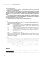
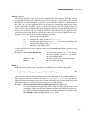
Contour plot produced
with the PROSA command plot of part of a
[13C-1H] COSY spectrum of a complex between the Antennapedia(C39S) homeodomain and a DNA
14-mer (Qian et al.,
1993). The spectrum
shows correlations between 13C and 1H atoms of aromatic rings.
The default values
were used for all parameters of the plot
command.
1
( H) [data points]
The default values for the parameters α-size, α-offset, α-margin, α-label, and α-tics
depend on the format and are chosen such that the plot makes good use of the
available paper size. To use the default value for a parameter, an asterisk “ *” may
be specified.
power
replaces the data in the active dimension by its squared absolute value (power
2
spectrum): s → s .
predict method m n [ k b k e ]
calculates complex data points in the active dimension using linear prediction (see
p. 52) with the following parameters:
method
must be lpsvd in the present version of PROSA, i. e. the linear prediction coefficients are calculated with singular value decomposition.
m
Number of linear prediction coefficients in Eq. [16].
n
Number of predicted complex data points. For positive n, n addition-
26
Commands
al data points are appended at the end; for negative n, the n first
data points are replaced with data points obtained from linear prediction. The latter possibility is used for the correction of baseline
distortions that are caused by errors in the first time-domain data
points (see p. 52).
specify the range of data points used for the determination of linear
prediction coefficients in Eq. [16]. If k b and k e are not specified, the
program uses all available data points for the determination of linear prediction coefficients .
kb , ke
project n
projects the data along the last dimension. If n = 0 , the projection is given by the
data point with the largest absolute value (“skyline projection”). For a natural
number n, the projection p of the data points s k along the last dimension is computed according to
p =
n
∑ sgn sk
k
sk n .
[8]
re
replaces complex data in the active dimension by its real part. Real data remain
unchanged.
read format filename { n k [c]}
read format filename combine [ f 1 ] [ f 2 ]
reads a file with time- or frequency-domain data. In the first form, data in memory
are overwritten; in the second form, a linear combination of the data in memory
and in the input file is formed. The second form of the read statement is not allowed for files in vnmr format. The parameters have the following meaning:
format
= real
serial data file containing real numbers,
= integer
serial data file containing integers,
= swap
serial data file containing integers with reversed
byte ordering,
= text
data file that can be read with F ORTRAN-77 listdirected input,
= easy or xeasy submatrix 8- or 16-bit data file of the program
XEASY (Bartels et al., 1995),
= vnmr
data file in the format of the Varian VNMR program
(Varian Associates Inc., 1993).
filename
Name of the input data file . In the case of the format easy two files
will be read; a XEASY parameter file called filename .3D.param and
the data file filename .3D.8 or filename .3D.16, respectively, and the
system variables for calibration will be set according to the XEASY
27
Commands
parameter file .
Number of real or complex data points to read in dimension k. If a
“ c” follows the number n k , complex data are read, otherwise real
data are read. n k has to be specified with the formats real, integer,
swap, text, and (optionally) vnmr. If the number of points is not
given for a file in vnmr format, the program assumes a two-dimensional data set with complex data in both dimensions and one FID
per trace, and extracts the number of data points from the file header. In the case of the format easy the corresponding numbers are
read from the XEASY parameter file , and real data are read from the
data file . In its present version the program can handle 2D, 3D, and
4D data sets. A one-dimensional data set is formally treated as a
two-dimensional data set with a single row, i. e. by setting n 2 = 1 .
Linear combination coefficient for data in memory. Default value: 1.
Linear combination coefficient for data read from input file . Default
value: –1, i. e. by default the difference between the data in memory
and in the input file is formed.
nk
f1
f2
real
converts n complex data points z k in the active dimension into 2n real data points
r l according to r 2k – 1 = Re z k and r 2k = Im z k ( k = 1, …, n ). Real data remain
unchanged.
reduce region {region}
reduces the data matrix to the specified regions. The first region corresponds to the
active dimension, the second region corresponds to the second dimension etc. If the
number of regions is less than the number of dimensions of the data set, all data
points will be used from the remaining dimensions. Data points outside the specified regions are discarded. A region can be given in one of the following formats:
n
denotes the data point n,
m . . n includes the data points m, m + 1, …, n ,
m..
includes the data points m, m + 1, … up to the last data point,
..n
includes the data points 1, 2, …, n ,
*
stands for all data points.
reverse
reverses the order of (real or complex) data points in the active dimension:
s 1, s 2, …, s n → s n, s n – 1, …, s 1 .
n denotes the number of data points in the active dimension.
28
[9]
Commands
select {region}
selects the specified regions from the complete the data matrix. The first region
corresponds to the active dimension, the second region corresponds to the second
dimension etc. If the number of regions is less than the number of dimensions of
the data set, all data points will be used from the remaining dimensions. Data
points outside the specified regions remain in memory, and the complete data set
can be restored by a select statement without parameters, provided that the size
of the selected data was not changed. All PROSA statements can be applied to the
selected portion of the data in exactly the same way as for the complete data set.
A region can be given in one of the following formats:
n
denotes the data point n,
m . . n includes the data points m, m + 1, …, n ,
m..
includes the data points m, m + 1, … up to the last data point,
..n
includes the data points 1, 2, …, n ,
*
stands for all data points.
n and m always refer to the complete data set; the select statement cannot be used
recursively.
Examples: select 100..200 50..80
# selects the points 100, …, 200 in the
# active and the points 50, …, 80 in the
# second dimension
select * * 20
# selects plane 20 of a 3D spectrum
select
# uses again all data
shift m
shifts the data in the active dimension circularly by m points to the right:
s 1, s 2, …, s n → s n – m + 1, s n – m + 2, …, s n, s 1, s 2, …s n – m .
[10]
n denotes the number of data points in the active dimension. A circular shift by m'
data points to the left is achieved with m = – m' or m = n – m' . m is an integer
expression that is interpreted modulo n and in which a lowercase k may denote an
index that runs over all data points in the passive dimensions.
Example: shift n/2-nint(real(n-1)/(ndata(perm(2))-1)*(k-1)+1)
In a two-dimensional spectrum with a diagonal through the lower left
and upper right corners, this command shifts the diagonal to the centre of the spectrum. Subsequently, the diagonal may be removed using
the smooth command (Friedrichs et al., 1991).
29
Commands
smooth n function [m] {option}
smooths the data in the active dimension by computing the moving average s k
over the n preceding and n following data points s k , that are weighted with the
given function. In the function f k a lowercase k stands for the index that runs from
– n to n.
f –n s k – n + … + f 0 s k + … + f n s k + n
s k = ---------------------------------------------------------------------------------------f –n + … + f 0 + … + f n
[11]
The following options are possible:
option
= extrapolate computes the m ≥ n data points in the border
regions by quadratic extrapolation of the smoothed
data,
= circular
assumes periodic data to smooth the border
regions,
= linear
uses only the available data points for smoothing
in the border regions (e. g. for the smoothed data
point 2 the data points 1, 2, 3, …, 2 + n ),
= replace
replaces the data by the smoothed data,
= subtract
subtracts the smoothed from the original data.
The parameter m has only a meaning with the option extrapolate. By default, the
options extrapolate and replace are set.
Example: smooth 20 cos(0.5*$pi/19*k) 22 extrapolate subtract
is a method to suppress signals with zero frequency, for example the
residual water signal. The data are extrapolated in the border regions
over more data points than used in the smoothing in order to avoid using the first two data points which are often corrupted. This method is
conveniently implemented in the macro suppress (see p. 39)
status [max] [full] [silent] [data]
displays information about the size and organization of the current data set. With
the option max, also the maximum absolute value is calculated and assigned to
the system variable max. With the option full, also the maximum absolute value
and the noise level are calculated and assigned to the system variables max and
noise, respectively. The option silent suppresses the display, which is useful if the
system variables max and noise should be updated silently. With the option data
the data are written to standard output (if less than 2048 numbers).
write format filename {region}
writes part or all of the data into the output file called filename . The parameters
have the following meaning:
format
= real
serial data file containing real numbers,
= integer
serial data file containing integers,
= swap
serial data file containing integers with reversed
30
Commands
filename
region
byte ordering,
= text
text file written with FORTRAN-77 format (1PE12.4),
= easy8 or xeasy8 submatrix 8-bit data file for the program X EASY,
= easy16 or xeasy16 submatrix 16-bit data file for X EASY.
Name of the output data file . In the case of the formats easy8,
xeasy8, easy16, xeasy16, easy, and xeasy two files will be written; a XEASY parameter file called filename .3D.param and the data
file filename .3D.8 or filename .3D.16, respectively. The calibration
entries of the parameter file are set to the corresponding values of
the system variables for calibration, delta, w0, and ppmmax (see
p. 33/35), if possible. Otherwise the spectrum will be treated as “uncalibrated” by X EASY.
Regions of the data set that are written into the output file . The first
region corresponds to the active dimension, the second region corresponds to the second dimension etc. If the number of regions is less
than the number of dimensions of the data set, all data points will
be used from the remaining dimensions. A region can be given in
one of the following formats:
n
denotes the data point n,
m..n
includes the data points m, m + 1, …, n ,
m..
includes the data points m, m + 1, … up to the last
data point,
..n
includes the data points 1, 2, …, n ,
*
stands for all data points.
Optionally, a region may be followed by “ r” or “ i” to indicate that in
the given dimension only the real or imaginary part, respectively, of
a complex data set should be written into the output file .
___________________________
31
Commands
32
Variables
Variables
The command line interpreter of the program PROSA allows the use of variables
that are similar to shell-variables in the UNIX operating system (see p. 16). The following is a list of all system variables specific to the program PROSA. System variables associated with the command line interpreter are explained on p. 16–19.
check
determines whether PROSA statements that change the data matrix are only
checked for errors or actually executed. Statements are executed if check is not
set or equal to NULL, otherwise, i. e. if one or several check options are set, statements are checked for different types of errors without doing the calculation. The
following options are possible:
memory
Insufficient memory or workspace size is an error .
file
Input data files that do not exist, or output data files that cannot be
opened or created result in an error.
command
All other errors (syntax errors, for instance) are reported.
The option command is always active. To determine the memory and workspace
size required for the execution of a macro it is useful not to set the option memory,
and to examine after the test the system variables usedsize and usedwork. If,
during the execution of a macro, a new data file is written and later read again,
the option file should not be set because the attempt to test the existence of the
file results in an error that would not occur if the macro is really executed (not just
tested). The most convenient way to test macros before execution is to use the standard macro job (see p. 38).
delta(k)
denotes the time or frequency increment between two data points in dimension k
(in seconds for the time-domain, in Hertz for the frequency-domain). If a data file
in the format of the program XEASY (Bartels et al., 1994; see p. 27) is read, the system variables delta(k) are set according to the values in the XEASY parameter file ,
and updated during Fourier transformation.
dim
denotes the active dimension and is write-protected.
33
Variables
icmplx(k)
equals 1 if the data in dimension k are real, and 2 if the data in dimension k are
complex. This variable is write-protected.
m
denotes the product of the numbers of real data points in the passive dimensions
and is write-protected.
max
denotes the maximal absolute value of the data and is write-protected. max is only
calculated and assigned with the statement status full.
maxsize and maxwork
denote the available memory and workspace sizes in words (see p. 9), respectively,
and are write-protected.
n
denotes the number of real or complex data points in the active dimension and is
write-protected.
ndata(k)
denotes the number of real or complex data points in dimension k and is write-protected. ndata($dim) is equivalent to n.
ndim
denotes the number of dimensions and is write-protected.
noise
denotes the noise level and is write-protected. noise is only calculated and assigned with the statement status full. An estimate of the median of the absolute
values of the data points is used for the noise level.
perm
denotes the current order of dimensions and is write-protected. perm(1) is equivalent to dim and denotes the active dimension.
34
Variables
phi0 and phi1
denote the constant ( φ 0 ) and linear ( φ 1 ) phase correction parameters (see Eq.
[23]). phi0 and phi1 are calculated and assigned with the statement autophase
but can also be set by the user.
pi
has the value 3.141593 and is write-protected.
ppmmax(k)
denotes the chemical shift (in ppm) of the first data point in dimension k. If a data
file in the format of the program XEASY (Bartels et al., 1994; see p. 27) is read, the
system variables ppmmax(k) are set according to the values in the XEASY parameter file .
timing
is a system variable to control the reporting of CPU times. CPU times are given
for all commands (except those that are built into the command line interpreter)
that need more seconds of CPU time than the value of timing indicates.
usedsize and usedwork
denote the used memory and workspace sizes in words. At the beginning of a PROSA
session both variables have the value 0. The execution of every subsequent statement increases these variables according to the necessary memory and workspace
sizes. The variables usedsize and usedwork can also be altered explicitly by the
user.
w0(k)
denotes the spectrometer frequency (in MHz) in dimension k. If a data file in the
format of the program XEASY (Bartels et al., 1994; see p. 27) is read, the system
variables w0(k) are set according to the values in the XEASY parameter file .
___________________________
35
Variables
36
Macros
Macros
This chapter gives an alphabetical list of the standard macros that are provided
with the program PROSA. The general initialization macro init is explained in the
chapter on the command line interpreter (see p. 19).
dummycal
sets the system variables delta(k), ppmmax(k) and w0(k) (see p. 33/35) to default values (delta(k) = w0(k) = 1000.0 and ppmmax(k) = number of data points
in dimension k). It thus avoids that XEASY treats the spectrum as “uncalibrated.”
cfl
cfl
cfl
cfl
att fl att n τ baseset m [ n 0 n b ] [ φ 1 ]
att derivative n τ baseset m [ n 0 n b ] [ φ 1 ]
att iterative [{region} -] baseset m [ n 0 n b ] [ φ 1 ]
att manual [{region} -] baseset m [ n 0 n b ] [ φ 1 ]
(“convenient FLATT”) flattens the baseline in the frequency-domain of the active dimension (see p. 23) using standard base function sets. It thus provides a convenient interface to the flatten command (see p. 23). The parameters n, τ and region
have the same meaning as for the flatten command. The other parameters define
the base function set:
baseset
denotes the set of base functions used to represent baseline distortions. The following choices are possible:
baseset
Base functions ( t = ( k – n b + 2 ) ⁄ n 0 , k = 1, …, n )
cft
1, cos 2πt, sin 2πt, …, cos 2πt ( m – 1 ), sin 2πt ( m – 1 )
rft
1, cos πt, sin πt, …, cos πt ( m – 1 ), sin πt ( m – 1 )
cftw
same as cft, plus Lorentzian functions to account for
contributions from the water line
rftw
same as rft, plus Lorentzian functions to account for
contributions from the water line
polynom
polynomial of order m
The methods cft and rft use trigonometric functions that correspond to the first m data points after complex and real Fourier
37
Macros
transformation, respectively. The additional Lorentzian functions
used in the basesets cftw and rftw assume that the water signal is
located in the middle of the spectrum (before a possible strip transform).
m
determines the number of base functions used to represent baseline
distortions. There will 2m – 1 base functions with the methods cft
and rft, 2m + 1 base functions with the methods cftw and rftw, and
m base functions with the method polynom.
n0 , nb
specifies that the present data in the active dimension represent a
strip out of a total of n 0 data points starting at data point n b . By
default, the values n 0 = n and n b = 1 are used (n denotes the
number of data points in the active dimension).
φ1
denotes the linear phase correction parameter used for phase correction.
The parameters n 0 , n b and φ 1 are not allowed when using the baseset polynom.
hilbert
performs a Hilbert transformation (Ernst, 1969) in the active dimension. Real
data are converted to complex data such that the real part remains unchanged and
the Kramers-Kroning relations are fulfilled.
im
replaces complex data in the active dimension by its imaginary part. Real data remain unchanged.
job macro {parameter}
checks for errors in the macro without executing the actual calculation and, provided that there is no error, executes the macro afterwards. The value of the system variable check (see p. 33) determines the type errors that are detected. By
default, i. e. if check has the value NULL when the macro is called, check will
be set to command file . If no error is detected, the memory and workspace sizes
necessary for the execution of the macro are displayed and the execution of the
macro is started if sufficient memory and workspace is available. In case of an error, the values of all global variables are listed and the program is stopped. The
macro must not contain statements such as quit that stop the program. job is particularly useful to execute macros in batch jobs.
38
Macros
phase φ 0 [ φ 1 ]
applies a phase correction according to Eq. [23] and the given constant ( φ 0 ) and
linear ( φ 1 ) phase correction parameters. The values of φ 0 and φ 1 must be given in
degrees. If the phase correction parameters are known, it is in general more efficient to use them together with the Fourier transformation (see p. 24) than to call
the macro phase.
reduceppm region {region}
works as the statement reduce (see p. 28), except that the regions must be specified in ppm units instead of points. This macro can only be used if the system variables delta(k), ppmmax(k) and w0(k) (see p. 33/35) are set.
savequit {filename }
displays the values of all global variables, writes the current data in real format
into the file called filename (by default, savequit.out) and stops the program.
This macro is a useful error handler for long calculations.
Example: set erract=savequit
sets savequit as error handling routine.
scale method intensity
scales the data such that in the case method = max the maximal absolute intensity
and in the case method = noise the noise level is set to the given intensity. The default intensity is 500’000 for the maximal absolute intensity and 100 for the noise
level, respectively.
selectppm {region}
works as the statement select (see p. 29), except that the regions must be specified
in ppm units instead of points. This macro can only be used if the system variables
delta(k), ppmmax(k) and w0(k) (see p. 33/35) are set.
suppress [weight [n]]
suppresses signals of zero frequency (the water line, for instance) by subtracting
smoothed time-domain data from the original time-domain data using the statement smooth (see p. 30). The smoothed data are calculated from the original data
according to Eq. [11]. The following weights are possible:
weight
cos
weighting function
f k = cos ( πk ⁄ ( 2 ( n + 1 ) ) )
gauss
fk = e
equal
fk ≡ 1
–4 ( k ⁄ n )
2
name
cosine weighting
Gaussian weighting
equal weighting
39
Macros
window type {parameter}
applies commonly used window functions (DeMarco & Wüthric h, 1976; Ernst et al.,
1987):
type
parameter
cos
–
window function
name
cos ( πt ⁄ 2 )
cos2
–
cos ( πt ⁄ 2 )
exp
L
e
cosine window
2
cosine squared window
– πLn∆t
exponential line broadening
– πLn∆t ( 1 – t ⁄ 2G )
Lorentz-Gauss transformation
gauss
LG
e
hamming
–
0.54 + 0.46 cos πt
Hamming window
hanning
–
0.5 + 0.5 cos πt
“Hanning” window
sin
φ
sin2
φ
sin ( φ – ( φ – π )t )
sin ( φ – ( φ – π )t )
shifted “sine-bell”
2
shifted “squared sine-bell”
The symbols in the table have the following meaning:
t = ( k – 1 ) ⁄ n , where k = 1, …, n runs over all n data points in the active dimension.
L
denotes the line broadening in Hertz.
G
denotes the maximum of the Lorentz-Gauss window function at
t = G.
∆
denotes the time increment in seconds, i. e. the value of the system
variable delta(active) (see p. 33).
φ
denotes the shift of the sine-bell or squared sine-bell in degrees (for
example, window sin 90 is equivalent to window cos).
___________________________
40
Examples
Examples
This chapter illustrates the use of PROSA with some practical examples of the processing of 2D and 3D data sets. The program can be used in three different ways:
The user may enter statements interactively.
The program can execute a sequence of statements contained in a macro file .
This strategy is shown in two examples (see p
A customized user interface may be created with the help of macros and the
“ask”-command.
The first example shows the data processing of a 2D [1H,1H]-NOESY data set of
the basic pancreatic trypsin inhibitor (BPTI). The PROSA commands are printed in
bold, and comments are printed in Helvetica.
set timing=1
Show the CPU time for commands that take more than1s of CPU time
read swap /files/nmr/vd/ser 1024c 100c
The time-domain data consist of 1024 complex data points in the first
(aquisition) dimension, and 100 complex data points in the second, indirect dimension. The data are stored as integer numbers with inverted
byte-ordering in a serial file called /files/nmr/vd/ser (see p. 27).
status
suppress cos 30
Show the size and organization of the data
The residual water signal (that has frequency zero in the aquisition dimension) is suppressed using the macro suppress (see p. 39).
print
print “-------- Dimension 1 --------”
Processing of the aquisition dimension
print
multiply 0.5 1
Scale the first data point by 1/2
window cos
Cosine window (see p. 40)
ft 1024
Fourier transformation with zero-filling to 1024 complex data points
status
Show the size and organization of the data
print
print “-------- Dimension 2 --------”
Processing of the second dimension
print
dimension 2
Transposition that activates the second dimension
41
Examples
multiply -1 2 $n 2
Change sign of every second data point (“States-TPPI”)
window cos
Cosine window (see p. 40)
ft 256
Fourier transformation with zero-filling to 256 complex data points
print
print "-------- Phase correction --------"
print
dimension 1
Re-activate the aquisition dimension
autophase 10 2.0 10.0 10 0
Automatic phase correction (see p.21)
re
Discard imaginary part of the aquisition dimension
dimension 2
Transposition that activates the second dimension
autophase 6 2.0 6.0 10
Automatic phase correction (see p.21)
re
Discard imaginary part
print
print "-------- Baseline correction --------"
print
dimension 1
Transposition that activates the first dimension
cflatt cft 10 6.0 3
Baseline correction using the FLATT method (see p.23/37/54) with a
half-width of 10 data points and a threshold parameter τ = 6 for the determination of pure-baseline regions. The basis functions that are used
to represent the baseline distortions are the (5) trigonometric functions
that correspond to the first 3 time-domain data points.
dimension 2
cflatt cft 6 6.0 3
Transposition that activates the second dimension
Baseline correction in the second dimension
dimension 1 2
Restore original order of dimensions
dummycal
scale noise 100
Scale data to a noise level of 100
status full
Show the size, noise level, and maximal intensity of the data
write easy16 /home/vd/noesy
Write an output spectrum file /home/vd/noesy.3D.16 and a parameter
file /home/vd/noesy.3D.param for XEASY.
Assuming that the above sequence of PROSA commands is stored in a macro file
called noesy.pro, the data processing is executed as follows (the statements are displayed before execution in the form macro: statement; informative output of the program starts with “. . .” and is indented):
prosa
PROSA, version 2.4 (Sun)
Memory size
:
Workspace size:
4456448 words (17408 kbytes)
4202496 words (16416 kbytes)
... Ready.
job noesy
... Checking the macro "noesy":
42
Examples
job: noesy
(Output from the check phase is omitted.)
... "noesy" checked. The execution of the macro requires
1052672 words of memory and 1049088 words of workspace.
job: noesy
noesy: read swap /files/nmr/vd/ser 1024c 100c
... File "/files/nmr/vd/ser" read.
(CPU time: 3.8 s, total CPU time: 4.3 s)
noesy: status
... Occupied memory
:
410000 words (9 %)
Dimension 1
:
1024 complex points
Dimension 2
:
100 complex points
Order of dimensions : 1 2
noesy: suppress cos 30
suppress: smooth 30 cos(0.5*3.141593/(30+1)*k) 30+3 extrapolate
subtract
... Smoothed data with extrapolated border regions subtracted.
(CPU time: 16.2 s, total CPU time: 20.8 s)
--------
Dimension 1
--------
noesy: multiply 0.5 1
... Data multiplied.
noesy: window cos
window: multiply cos(3.141593/(2*1024)*(k-1))
... Data multiplied.
noesy: ft 1024
... Complex Fourier transform performed.
(CPU time: 4.0 s, total CPU time: 25.8 s)
noesy: status
... Occupied memory
:
410000 words (9 %)
Dimension 1
:
1024 complex points
Dimension 2
:
100 complex points
Order of dimensions : 1 2
--------
Dimension 2
--------
noesy: dimension 2
... New order of dimensions: 2 1
noesy: multiply -1 2 100 2
... Data multiplied.
noesy: window cos
window: multiply cos(3.141593/(2*100)*(k-1))
... Data multiplied.
noesy: ft 256
... Complex Fourier transform performed.
(CPU time: 8.7 s, total CPU time: 36.4 s)
--------
Phase correction --------
noesy: dimension 1
... New order of dimensions: 1 2
43
Examples
(CPU time: 2.7 s, total CPU time: 39.1 s)
noesy: autophase 10 2.0 10.0 10 0
... Noise standard deviation : 2.249E+04
Number of peaks used
:
199
Constant phase correction:
-25.2 deg
Standard deviation
:
28.5 deg
Automatic phase correction applied.
(CPU time: 2.5 s, total CPU time: 41.7 s)
noesy: re
... Real part kept, imaginary part discarded.
noesy: dimension 2
... New order of dimensions: 2 1
noesy: autophase 6 2.0 6.0 10
... Noise standard deviation : 1.875E+04
Number of peaks used
:
414
Constant phase correction:
63.3 deg
Linear phase correction :
-129.0 deg
Standard deviation
:
8.2 deg
Automatic phase correction applied.
(CPU time: 5.1 s, total CPU time: 47.9 s)
noesy: re
... Real part kept, imaginary part discarded.
--------
Baseline correction --------
noesy: dimension 1
... New order of dimensions: 1 2
noesy: cflatt cft 10 6.0 3
cflatt: flatten flatt 10 6.0 1 sin(6.135924E-03*(-1+k))
cos(6.135924E-03*(-1+k)) sin(1.227185E-02*(-1+k))
cos(1.227185E-02*(-1+k))
... Average size of baseline regions: 63.2 %
Minimal size of baseline regions: 48.2 %
Baseline corrected.
(CPU time: 19.9 s, total CPU time: 69.0 s)
noesy: dimension 2
... New order of dimensions: 2 1
noesy: cflatt cft 6 6.0 3
cflatt: flatten flatt 6 6.0 1 sin(2.454370E-02*(-1+k))
cos(2.454370E-02*(-1+k)) sin(4.908740E-02*(-1+k))
cos(4.908740E-02*(-1+k))
... Average size of baseline regions: 84.0 %
Minimal size of baseline regions: 55.5 %
Baseline corrected.
(CPU time: 17.3 s, total CPU time: 87.4 s)
noesy: dimension 1 2
... New order of dimensions: 1 2
noesy: dummycal
noesy: scale noise 100
scale: status full
... Occupied memory
:
262400 words (6 %)
Dimension 1
:
1024 real points
Dimension 2
:
256 real points
Order of dimensions : 1 2
44
Examples
Maximal magnitude
: 1.64E+07
Noise magnitude
: 3.40E+03
(CPU time: 1.0 s, total CPU time: 89.3 s)
scale: multiply (100)/3404.98
... Data multiplied.
noesy: status full
... Occupied memory
:
262400 words (6 %)
Dimension 1
:
1024 real points
Dimension 2
:
256 real points
Order of dimensions : 1 2
Maximal magnitude
: 4.81E+05
Noise magnitude
: 1.00E+02
(CPU time: 1.1 s, total CPU time: 90.7 s)
noesy: write easy16 /home/vd/noesy
... File "/home/vd/noesy.3D.16" written.
(CPU time: 4.9 s, total CPU time: 95.7 s)
... Ready.
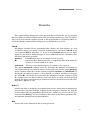
The resulting spectrum is shown in the Figure.
500
1000
200
200
100
100
Contour plot produced
with the PROSA command plot of part of a
NOESY spectrum of
BPTI. The data set was
processed as described
above.
500
1000
45
Examples
As an example for the processing of higher-dimensional datas sets, the following
shows the data processing of a three-dimensional 15N-correlated [1H, 1H] NOESY data
set:
read swap /tmp/SFS/angio.3d 1024c 150c 16c
The time-domain data consist of 1024 complex data points in the first
(aquisition) dimension, 150 complex data points in the second dimension, and 16 complex data points in the third dimension. The data are
stored as integer numbers with inverted byte-ordering in a serial file
called /tmp/SFS/angio.3d (see p.27).
suppress cos 30
The residual water signal (that has frequency zero in the aquisition dimension) is suppressed using the macro suppress (see p. 39).
print
print "-------- Dimension 1 --------"
print
multiply 0.5 1
window cos
ft 2048 1 1024
Processing of the aquisition dimension
Scale the first data point by 1/2
Cosine window (see p. 40)
The data are zero-filled to 2048 complex data points prior to Fourier
transformation, and only the left half of the resulting spectrum is retained (see p.24).
print
print "-------- Dimension 2 --------"
Processing of the second dimension
print
dimension 2
Transposition that activates the second dimension
multiply -1 2 $n 2
Change sign of every second data point (“States-TPPI”)
window cos
Cosine window (see p. 40)
ft 256 1 256 90 -180
The data are zero-filled to 256 complex data points prior to Fourier
transformation, a constant phase correction of 90˚ and a linear phase
correction of –180˚ are applied, and only the real part of the spectrum
is retained (see p.24).
dimension 1
Re-activate the aquisition dimension
autophase 14 2.0 8.0 8 0
Automatic phase correction (see p.21)
re
Discard imaginary part of the aquisition dimension
print
print "-------- Dimension 3 --------"
Processing of the third dimension
print
dimension 3
Transposition that activates the third dimension
multiply -1 2 $n 2
Change sign of every second data point (“States-TPPI”)
predict lpsvd 5 16
Append 16 complex data points by linear prediction with 5 coefficients
(see p.26).
46
Examples
window cos2
Cosine squared window (see p. 40)
ft 32
Fourier transformation with zero-filling to 32 complex data points
autophase 4 2.0 6.0 5
Automatic phase correction (see p.21)
re
Discard imaginary part
print
print "-------- Baseline correction --------"
print
dimension 1
cflatt cft 10 6.0 3 2048 1
Activate the aquisition dimension
Baseline correction using the FLATT method (see p. 23/37/54) with a
half-width of 10 data points and a threshold parameter τ = 6 for the determination of pure-baseline regions. The basis functions that are used
to represent the baseline distortions are the (5) trigonometric functions
that correspond to the first 3 time-domain data points. To correctly generate these basis functions the command must be provided with the information that the present data constitutes a strip taken out of the
complete size of 2048 complex points starting at data point 1 (cf. the
command ft 2048 1 1024 above; see p. 37).
dimension 2
Activate the second dimension
cflatt cft 4 6.0 3
Baseline correction in the second dimension
dimension 3
Activate the third dimension
cflatt cft 3 6.0 3
Baseline correction in the third dimension
dimension 1 2 3
Restore original order of dimensions
dummycal
Set dummy calibration parameters for XEASY
write easy16 /tmp/SFS/vd/hxnoe3d
Write an output spectrum file /tmp/SFS/vd/hxnoe3d.3D.16 and a parameter file /tmp/SFS/vd/hxnoe3d.3D.param for XEASY.
___________________________
47
Examples
48
Algorithms
Algorithms
Spectrum file f ormats
The program PROSA supports various formats for the storage of time- or frequencydomain data. The formats are summarized in the following table:
format
order
bits/point
coding
number format
real
serial
32
binary
real
integer
serial
32
binary
integer
swap
serial
32
binary
integera
text
serial
13 × 8 b
ASCII
real
xeasy8
submatrix
8
binary
logarithmic
xeasy16
submatrix
16
binary
real
vnmrc
serial
16 or 32d
binary
integer or reale
a With inverted byte-ordering.
b On output. On input, the number of bits/point is variable.
c Only for input.
d Depending on the status bit S_32 in the file header.
e Depending on the status bit S_FLOAT in the file header.
For all formats except vnmr the data file contains only the data points themselves
without any headers or other information. For the formats xeasy8 and xeasy16 a separate parameter file accompanies the data file (see below).
In a serial data file the data points of the first dimension (usually the acquisition
dimension) are stored sequentially. Next, the data are ordered by the second dimension etc. For example, the data points s kl ( k = 1, …, m ; l = 1, …, n ) of a two-dimensional data set with m points in the first dimension and n points in the second
dimension are stored in the following order:
s 11, …, s m1, s 12, …, s m2, …, s 1n, …, s mn
[12]
For complex data, the real part is stored followed by the imaginary part.
In a submatrix data file (formats xeasy8 and xeasy16) the data set is split into
submatrices with sizes as given in the accompanying parameter file (Bartels et al.,
49
Algorithms
1995; Xia & Bartels, 1993). Within each individual submatrix the data are ordered as
in a serial file , and the submatrices as a whole are ordered in the same way as the data
points of a serial file . On output, the program PROSA uses for a data set with n real
data points in a given dimension a submatrix size of n ⁄ 8 (but at least 1) in the corresponding dimension. If necessary, the submatrix size in the active dimension is increased to the next integer multiple of 4 or 2 for the formats xeasy8 or xeasy16,
respectively, in order to align the submatrices at word boundaries. On input, the submatrix size in the active dimension must be an integer multiple of 2 or 4 for the formats xeasy8 or xeasy16, respectively. For the submatrix sizes in the other
dimensions there is no such condition.
In the format real the data are stored in the binary floating point number format
of the given computer with one real data point per (32 bit) word. Data files written
with real format contain the data with full accuracy but are machine dependent. In
the format integer the data are stored in the binary integer number format of the given computer with one real data point per (32 bit) word. In principle integer format
files are also machine dependent but because most computers use the same binary representation of integer numbers, such files can in general be used on various computers.
In the format swap the data are stored with inverse byte-ordering in the binary integer number format of the given computer with one real data point per (32 bit) word, i.
e. the 4 bytes
of an integer number are stored in the order
This format is useful to read integer data from a computer that uses inverse byte-ordering
with respect to the given machine but otherwise identical representation of integers.
For example, Bruker X32 computers use inverse byte-ordering when compared to Sun,
Convex, and NEC-SX3 computers. Text is a simple ASCII format using the FORTRAN77 format (1PE12.4) for output and list-directed (“free format”) FORTRAN-77 input.
This format is primarily designed to store small (1D) data sets for use with simple simulation programs or graphics programs such as GNUPLOT. The format xeasy8 uses a
logarithmic representation of the data with 1 byte per real data point (Bartels et al.,
1995; Xia & Bartels, 1993). For a given data point s k the program first determines the
integer l that minimizes the expression
sk – 2
(i. e. l ≈
2log
l
[13]
s k ) and then stores in one byte
e k = min(l + 1, 47),
= 95 – min(l, 47) ,
if s k ≥ 0;
[14]
if s k < 0.
47
46
This format can represent numbers approximately in the range – 2 ≤ s k ≤ 2 , i. e.
7
6
– 1.2 10 ≤ s k ≤ 8.4 10 with a relative error of less than 20%. The format xeasy16
uses a 16 bit floating point format with the “exponent” e k given by Eq. [14] in the lower
valued byte and the mantissa
sk
a k = 721 --------l – 615,
2
50
if l ≠ 0
[15]
Algorithms
( a k = 0 if l = 0 ) in the higher valued byte (Bartels et al., 1995; Eccles et al., 1991; Xia
& Bartels, 1993). This format can represent numbers in the same range as the format
xeasy8 but with a relative error of less than 1%.
A xeasy8 or xeasy16 format data set consists of a data file file .3D.8 or file .3D.16,
respectively, and a parameter file file .3D.param that contains information about the
type, size, and organization of the data file . A parameter file written by PROSA for a
two-dimensional data set has the following entries:
Version .......................
Number of dimensions ..........
16 or 8 bit file type .........
Spectrometer frequency in w1 ..
Spectrometer frequency in w2 ..
Spectral sweep width in w1 ....
Spectral sweep width in w2 ....
Maximum chemical shift in w1 ..
Maximum chemical shift in w2 ..
Size of spectrum in w1 ........
Size of spectrum in w2 ........
Submatrix size in w1 ..........
Submatrix size in w2 ..........
Permutation for w1 ............
Permutation for w2 ............
Folding in w1 .................
Folding in w2 .................
Type of spectrum ..............
1
2
16
600.0
600.0
10.0
10.0
10.0
10.0
256
301
32
38
2
1
RSH
RSH
?
(always 1 in PROSA)
(ndim)
(8 for xeasy8, 16 for xeasy16)
(w0(2))
(w0(1))
(delta(2)/w0(2) * ndata(2))
(delta(1)/w0(1) * ndata(1))
(ppmax(2))
(ppmax(1))
(ndata(2))
(ndata(1))
(see above)
(see above)
( ω 1 -dimension)
( ω 2 -dimension)
(always RSH in PROSA)
(always RSH in PROSA)
(always ? in PROSA)
Given in parentheses are the corresponding PROSA system variables (see p.
The parameter files for three- and four-dimensional data sets contain similar entries
for the additional dimensions.
Data files in vnmr format start with a 32 byte file header followed by blocks consisting of a block header and sequentially stored data (Varian Associates, 1993). The
organization of the data is extracted from the file header, block headers are simply
skipped by the program PROSA.
Noise level
Several PROSA statements (for example autophase and plot) use a noise level to
automatically adapt parameters to the scaling of data. The program PROSA uses an approximation of the median (Press et al., 1986) of the absolute value of the real data
points to estimate the noise level. To improve the efficiency of the noise level calculation, only about 10% or 1% of the data points are taken into account for the noise level
calculation if the data set includes more than 105 or 106 data points, respectively.
51
Algorithms
Linear prediction
In PROSA, linear prediction (Olejniczak and Eaton, 1990; Stephenson, 1988; Zhu
and Bax, 1990) is used to reduce effects caused by discrete Fourier transformation of
truncated time-domain signals, i.e., primarily line broadening and the appearance of
sidelobes. The linear prediction method is based on the assumption that a data point
s k can be written as a linear combination of the m preceding data points
s k – m, …, s k – 1 :
m
∑ al sk – l .
sk =
[16]
l=1
For a superposition of at most m damped oscillations with amplitudes A α , phases φ α ,
frequencies ω α and dampings Γ α that is sampled in time steps ∆t ,
sk =
∑ Aα e
iφ α – ( Γ α + iω α )k∆t
e
,
[17]
α
this assumption is fulfilled, and the zeros z 1, …, z m of the polynomial
m
1–
∑ al z
l=1
l
[18]
( Γ α + iω α )∆t
are related to the frequencies and damping factors by z α = e
. The linear prediction coefficients a 1, …, a m are determined by application of Eq. [16] to the measured data using singular value decomposition (Barkhuijsen et al., 1987; Kumaresan
and Tufts, 1982; Press et al., 1986). Since each individual coefficient represents one
frequency component, it is necessary to have an approximate estimate of the number
of frequencies included in the time domain signal, and additional coefficients are needed to account for the noise. Singular value decomposition uses an overdetermined system of equations, and the maximal number of coefficients can be as high as one half of
the number of complex data points. To ensure that the predicted signal is stable, the
roots of the characteristic polynomial [18] of the linear prediction coefficients are calculated. Following conventional use of linear prediction, PROSA takes all roots into account and guarantees a stable predicted signal by reflecting the roots z about the unit
2
circle, z → z ⁄ z , if necessary (Press et al., 1986). Although this procedure incorporates noise into the predicted data, the results do usually not differ significantly from
those obtained when putative noise roots are eliminated, because the noise roots usually lead to rapidly decaying components of small intensity in the predicted data
(Stephenson, 1988).
Since baseline distortions are primarily caused by errors in the measurement of
the first few time-domain data points (Otting et al., 1986), the backward linear prediction implemented in PROSA can be used to restore this corrupted part of the signal, and
is thus also a suitable method for baseline correction (Marion and Bax, 1989). When
compared with baseline correction procedures that work in the frequency-domain (Dietrich et al., 1991; Güntert and Wüthric h, 1992; Pearson, 1977), an advantage of this
method is that the baseline correction is performed at the beginning rather than at the
52
Algorithms
end of the data processing, which may improve the results of other processing steps
that rely on having a flat baseline .
Automatic phase correction
The automatic phase correction routine developed for PROSA determines the constant and linear phase correction parameters φ0 and φ1 by first searching the 1D crosssections of the power spectrum for strong, well separated peaks. Then, in the phasesensitive spectrum, the sum S(φ 0, φ 1) of the difference between the squared real and
imaginary parts of the normalized integral over the peak region in the phase-corrected
spectrum, Î p ,
S(φ 0, φ 1) =
∑ [ ( ReÎ p )
2
2
– ( ImÎ p ) ]
[19]
p
with
I p –i ( φ0 + φ1 ω p )
Î p = -------- e
Ip
[20]
is maximized. Ip denotes the integral over the region of the peak p in the spectrum before phase correction, and ωp denotes the normalized position of peak p ( 0 ≤ ω p ≤ 1 ).
The summation runs over all the peaks that were found to be acceptable for the purpose of the phase correction (see below). The maximum of S(φ 0, φ 1) is obtained by selecting the linear phase correction φ1 such that the function [21],
s(β) =
Ip

∑  -------Ip 
2 – 2iβω
p
e
,
[21]
p
has its maximum absolute value at β = φ 1 . The constant phase correction is given by
1
φ 0 = --- arg s (φ 1) ,
2
[22]
where arg s is the argument of the complex number s. Because s(β) has in general multiple local maxima, PROSA determines φ1 by a one-dimensional grid search with a step
size ∆β (usually, ∆β = 1˚ ). The phase-corrected spectrum ŝ 1, …, ŝ n is obtained from
the original spectrum s 1, …, s n by
ŝ k = s k e –i ( φ0 + φ1 t )
with
k–1
t = ------------ .
n–1
[23]
The method can be used for spectra containing both positive and negative peaks (but
of course not for anti-phase multiplets).
In practice, to determine peak positions in 1D cross-sections of the power spectrum, the program first identifies all local maxima that are more than κ times above
53
Algorithms
the noise level of the power spectrum (typically, κ = 10). For each maximum the corresponding boundaries for peak integration are set at the first data points on either side
that are lower than either 10% of the maximal peak intensity or twice the noise level.
To decide which of the maxima correspond to suitable peaks for use in the automatic
phase correction, the following criteria are checked: (i) The width of the integration
area must be smaller than a predetermined value u. (ii) To exclude overlapping peaks
the average intensity in the regions of width u ⁄ 4 adjoining the integration area to the
left and to the right must be either below 10% of the maximal peak intensity or below
twice the noise level. (iii) An upper limit, v, is imposed on the number of peaks that
may have the same coordinates along one frequency axis (typically, v =
If v is
exceeded, the program will only retain the v highest peaks so that the phasing cannot
be dominated by one or several small spectral regions. The results of the automatic
phase correction do not depend critically on the selection of the three parameters κ, u,
and v. We found that the value of κ should be decreased for spectra with low signal-tonoise ratio, that the maximal peak width, u, should account for the increased line
widths in power spectra and that v can be reduced when a spectrum contains a large
number of peaks. Usually the number of one-dimensional peaks included for the phase
correction of a 3D spectrum is of the order 1000, which renders the method robust
against instabilities that might arise if only a small number of peaks were used, be it
because of low signal-to-noise ratio, poor digital resolution, peak overlap, or occasional
inclusion of artifactual peaks.
Baseline correction
Baseline correction in the frequency domain is performed for each 1D cross-section
by first identifying regions of “pure-baseline” (Güntert and Wüthric h, 1992) and then
subtracting a function which is best-fitted to the pure-baseline regions. The pure-baseline regions are identified either with modified versions of the FLATT procedure (Güntert and Wüthric h, 1992) or with the “derivative method” of Dietrich et al. (1991). For
a data point k with intensity s k , both methods yield a parameter, p k , which becomes
small if the data point k is located in a pure-baseline region, and large otherwise:
n
FLATT:
p k = min
a, b
∑
2
( s k + l – a – bl ) ,
n≥1
[24]
n≥0
[25]
l = –n
2
Derivative method: p k = ( s k + max(1, n) – s k – n ) ,
In Eq. [24], pk is determined by fitting a straight line, a + bl , to a stretch of 2n + 1 data
points centered about the data point k. For the data points near the boundaries of the
1D cross section, where p k is not defined by Eq. [24], p k has the same value as the
nearest data point inside the definition range. A minimal width for pure-baseline regions (Güntert and Wüthric h, 1992) is ensured by smoothing p k :
FLATT:
54
p k = min ( p k – n ⁄ 3, …, p k + n ⁄ 3 )
[26]
Algorithms
Derivative method: p k = max(min( p k, max( p k – 1, p k + 1)), min( p k – 1, p k + 1)) [27]
The definition of p k for the derivative method implies that any point of which both
neighbors belong to pure-baseline regions will also belong to it, and that there is no
point in a pure-baseline region for which both neighboring points do not belong to it
(Dietrich et al., 1991). A cutoff, pc, is then defined such that p k ≤ p c for one third of the
data points and p k > p c for two thirds of the data points, and all data points k that satisfy the relation p k ≤ τ p c are considered as pure baseline, where τ is a user-defined parameter (typically, τ = 4). Any linear combination of functions that can be written as
FORTRAN-77 arithmetic expressions may be used to represent the baseline distortions.
Usually, we use the constant and the trigonometric functions corresponding to the first
m time-domain data points (see Eq. [4] in Güntert and Wüthric h, 1992). The linear
least-squares fit to the pure-baseline regions is solved by standard techniques using
singular value decomposition (Press et al., 1986).
___________________________
55
Algorithms
56
References
References
Barkhuijsen, H., De Beer, R. & van Ormondt, D. (1987). Improved algorithm for noniterative
time-domain model fitting to exponentially damped magnetic resonance signals. J. Magn.
Reson. 73, Bartels, C., Xia, T., Güntert, P., Billeter, M. & Wüthric h, K. (1995). The program XEASY for computer-supported NMR spectral analysis. J. Biomol. NMR, in preparation.
DeMarco, A. & Wüthric h, K. (1976) Digital filtering with a sinusodial window function: An alternative technique for resolution enhancement in FT NMR. J. Magn. Reson. 24, Dietrich, W., Rüdel, C. H. & Neumann, M. (1991). Fast and precise automatic baseline correction of one- and two-dimensional NMR spectra. J. Magn. Reson. 91, Eccles, C., Güntert, P., Billeter, M. & Wüthric h, K. (1991). Efficient analysis of protein 2D NMR
spectra using the software package EASY. J. Biomol. NMR, 1, Ernst, R. R. (1969). Numerical Hilbert transform and automatic phase correction in magnetic
resomance spectroscopy. J. Magn. Reson. 1, Ernst, R. R., Bodenhausen, G. & Wokaun, A. (1987). The principles of nuclear magnetic resonance in one and two dimensions, Clarendon, Oxford.
Friedrichs, M. S., Metzler, W. J. & Mueller, L. (1991). Removal of diagonal peaks in two-dimensional NMR spectra by means of digital filtering . J. Magn. Reson. 95, Güntert, P. & Wüthric h, K. (1992). A new procedure for high-quality baseline correction of twoand higher-dimensional NMR spectra. J. Magn. Reson. 96, Güntert, P., Dötsch, V., Wider, G. & Wüthric h K. (1992). Processing of multi-dimensional NMR
data with the new software PROSA. J. Biomol. NMR, 2, Kießling, I. & Lowes, M. (1987). Programmierung mit FORTRAN-77, Teubner, Stuttgart.
Kumaresan, R. & Tufts, D. W. (1982). Estimating the parameters of exponentially damped sinusoids and pole-zero modeling in noise. IEEE Transactions on Acoustics, Speech, and Signal Processing, ASSP-30, Marion, D. & Bax, A. (1989). Baseline correction of 2D FT NMR spectra using a simple linear
prediction extrapolation of the time domain data. J. Magn. Reson. 83, Olejniczak, E. T. & Eaton, H. L. (1990). Extrapolation of time-domain data with linear prediction increases resolution and sensitivity. J. Magn. Reson. 87, Otting, G., Widmer, H., Wagner, G. & Wüthric h, K. (1986). Origin of t1 and t2 ridges in 2D NMR
spectra and procedures for suppression. J. Magn. Reson. 66, Pearson, G. A. (1977). A general baseline-recognition and baseline-flattening algorithm. J.
Magn. Reson. 27, Press, W. H., Flannery, B. P., Teukolsky, S. A., Vetterling, W. T. (1986). Numerical Recipes. The
art of scientific computing , Cambridge University Press, Cambridge.
Qian, Y. Q., Otting, G., Billeter, M., Müller , M., Gehring, W. & Wüthric h, K. (1993). NMR spectroscopy of a DNA complex with the uniformly 13C-labeled Antennapedia homeodomain and
structure determination of the DNA-bound homeodomain. J. Mol. Biol. 234, 57
References
Stephenson, D. S. (1988). Linear prediction and maximum entropy methods in NMR spectroscopy. Prog. NMR Spectrosc. 20, Varian Associates Inc. (1993). User programming VNMR 4.3, Palo Alto, California.
Wüthric h, K. (1986). NMR of Proteins and Nucleic Acids, Wiley, New York.
Xia, T. H. & Bartels, C. (1993). XEASY. ETH Automated Spectroscopy for X Window Systems.
User Manual, Institut für Molekularbiologie und Biophysik, ETH Züric h.
Zhu, G. & Bax, A. (1990). Improved linear prediction for truncated signals of known phase. J.
Magn. Reson. 90, ___________________________
58