Download Starting Excel 2007

Excel 2007
Microsoft® Office
Student Edition
Complete
DoubleTechs.com Remote Computer Repair
Table of Contents
The Fundamentals................................................................................................................................................. 10
Starting Excel 2007............................................................................................................................................... 11
What’s New in Excel 2007.................................................................................................................................... 12
Understanding the Excel Program Screen ........................................................................................................... 13
Understanding the Ribbon.................................................................................................................................... 14
Using the Office Button and Quick Access Toolbar .............................................................................................. 15
Using Keyboard Commands ................................................................................................................................ 16
Using Contextual Menus and the Mini Toolbar..................................................................................................... 17
Using Help ............................................................................................................................................................ 18
Exiting Excel 2007 ................................................................................................................................................ 20
Worksheet Basics ................................................................................................................................................. 21
Creating a New Workbook.................................................................................................................................... 22
Opening a Workbook............................................................................................................................................ 23
Navigating a Worksheet ....................................................................................................................................... 24
Entering Labels..................................................................................................................................................... 25
Entering Values .................................................................................................................................................... 26
Selecting a Cell Range ......................................................................................................................................... 27
Overview of Formulas and Using AutoSum ......................................................................................................... 28
Entering Formulas ................................................................................................................................................ 29
Using AutoFill........................................................................................................................................................ 31
Understanding Absolute and Relative Cell References ....................................................................................... 32
Using Undo, Redo and Repeat ............................................................................................................................ 33
Saving a Workbook .............................................................................................................................................. 35
Previewing and Printing a Worksheet .................................................................................................................. 37
Closing a Workbook ............................................................................................................................................. 38
Editing a Worksheet.............................................................................................................................................. 39
Editing Cell Contents ............................................................................................................................................ 40
Cutting, Copying, and Pasting Cells..................................................................................................................... 41
Moving and Copying Cells Using the Mouse ....................................................................................................... 43
Using the Office Clipboard.................................................................................................................................... 44
Using the Paste Special Command...................................................................................................................... 45
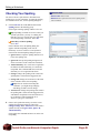
Checking Your Spelling......................................................................................................................................... 46
Inserting Cells, Rows, and Columns .................................................................................................................... 48
Deleting Cells, Rows, and Columns ..................................................................................................................... 49
Using Find and Replace ....................................................................................................................................... 50
Using Cell Comments........................................................................................................................................... 52
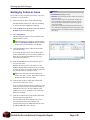
Tracking Changes................................................................................................................................................. 54
Formatting a Worksheet ....................................................................................................................................... 55
Formatting Labels................................................................................................................................................. 56
Formatting Values................................................................................................................................................. 57
Adjusting Row Height and Column Width ............................................................................................................ 58
Working with Cell Alignment ................................................................................................................................. 59
Adding Cell Borders, Background Colors and Patterns ....................................................................................... 60
Using the Format Painter...................................................................................................................................... 62
Using Cell Styles................................................................................................................................................... 63
Using Document Themes ..................................................................................................................................... 65
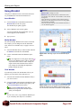
Applying Conditional Formatting .......................................................................................................................... 67
Creating and Managing Conditional Formatting Rules ........................................................................................ 69
Finding and Replacing Formatting ....................................................................................................................... 71
Creating and Working with Charts ...................................................................................................................... 72
Creating a Chart ................................................................................................................................................... 73
Resizing and Moving a Chart ............................................................................................................................... 75
DoubleTechs.com Remote Computer Repair
Page 3
Changing Chart Type............................................................................................................................................76
Applying Built-in Chart Layouts and Styles...........................................................................................................77
Working with Chart Labels....................................................................................................................................78
Working with Chart Axes ......................................................................................................................................80
Working with Chart Backgrounds .........................................................................................................................81
Working with Chart Analysis Commands .............................................................................................................82
Formatting Chart Elements...................................................................................................................................83
Changing a Chart’s Source Data..........................................................................................................................85
Using Chart Templates .........................................................................................................................................86
Managing Workbooks ...........................................................................................................................................87
Viewing a Workbook .............................................................................................................................................88
Working with the Workbook Window ....................................................................................................................90
Splitting and Freezing a Workbook Window.........................................................................................................91
Selecting Worksheets in a Workbook...................................................................................................................93
Inserting and Deleting Worksheets.......................................................................................................................94
Renaming, Moving and Copying Worksheets ......................................................................................................95
Working with Multiple Workbooks.........................................................................................................................97
Hiding Rows, Columns, Worksheets and Windows .............................................................................................98
Protecting a Workbook .......................................................................................................................................100
Protecting Worksheets and Worksheet Elements ..............................................................................................102
Sharing a Workbook ...........................................................................................................................................104
Creating a Template ...........................................................................................................................................106
Working with Page Layout and Printing ...........................................................................................................107
Creating Headers and Footers ...........................................................................................................................108
Using Page Breaks............................................................................................................................................. 110
Adjusting Margins and Orientation ..................................................................................................................... 112
Adjusting Size and Scale.................................................................................................................................... 113
Adding Print Titles, Gridlines and Headings ....................................................................................................... 114
Advanced Printing Options ................................................................................................................................. 116
More Functions and Formulas........................................................................................................................... 118
Formulas with Multiple Operators....................................................................................................................... 119
Inserting and Editing a Function.........................................................................................................................120
AutoCalculate and Manual Calculation ..............................................................................................................122
Defining Names ..................................................................................................................................................124
Using and Managing Defined Names.................................................................................................................126
Displaying and Tracing Formulas .......................................................................................................................128
Understanding Formula Errors ...........................................................................................................................130
Working with Data Ranges .................................................................................................................................132
Sorting by One Column ......................................................................................................................................133
Sorting by Colors or Icons ..................................................................................................................................135
Sorting by Multiple Columns...............................................................................................................................137
Sorting by a Custom List ....................................................................................................................................138
Filtering Data ......................................................................................................................................................140
Creating a Custom AutoFilter .............................................................................................................................141
Using an Advanced Filter....................................................................................................................................142
Working with Tables............................................................................................................................................144
Creating a Table..................................................................................................................................................145
Working with Table Size .....................................................................................................................................147
Working with the Total Row ................................................................................................................................149
Working with Table Data .....................................................................................................................................151
Summarizing a Table with a PivotTable..............................................................................................................153
Using the Data Form ..........................................................................................................................................154
Using Table Styles ..............................................................................................................................................155
DoubleTechs.com Remote Computer Repair
Page 4
Using Table Style Options...................................................................................................................................156
Creating and Deleting Custom Table Styles .......................................................................................................157
Convert or Delete a Table...................................................................................................................................159
Working with PivotTables...................................................................................................................................160
Creating a PivotTable .........................................................................................................................................161
Specifying PivotTable Data .................................................................................................................................162
Changing a PivotTable’s Calculation ..................................................................................................................163
Filtering and Sorting a PivotTable.......................................................................................................................164
Working with PivotTable Layout .........................................................................................................................165
Grouping PivotTable Items .................................................................................................................................167
Updating a PivotTable.........................................................................................................................................169
Formatting a PivotTable......................................................................................................................................170
Creating a PivotChart .........................................................................................................................................171
Analyzing and Organizing Data .........................................................................................................................172
Creating Scenarios .............................................................................................................................................173
Creating a Scenario Report................................................................................................................................175
Working with Data Tables ...................................................................................................................................176
Using Goal Seek.................................................................................................................................................178
Using Solver .......................................................................................................................................................179
Using Data Validation .........................................................................................................................................181
Using Text to Columns........................................................................................................................................183
Removing Duplicates..........................................................................................................................................185
Grouping and Outlining Data ..............................................................................................................................186
Using Subtotals ..................................................................................................................................................188
Consolidating Data by Position or Category.......................................................................................................190
Consolidating Data Using Formulas...................................................................................................................192
Working with the Web and External Data .........................................................................................................193
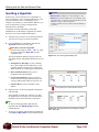
Inserting a Hyperlink...........................................................................................................................................194
Creating a Web Page from a Workbook.............................................................................................................195
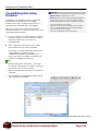
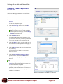
Importing Data from an Access Database or Text File .......................................................................................196
Importing Data from the Web and Other Sources ..............................................................................................198
Working with Existing Data Connections............................................................................................................200
Working with Macros ..........................................................................................................................................202
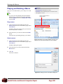
Recording a Macro .............................................................................................................................................203
Playing and Deleting a Macro ............................................................................................................................205
Adding a Macro to the Quick Access Toolbar.....................................................................................................206
Editing a Macro’s Visual Basic Code..................................................................................................................207
Inserting Copied Code in a Macro......................................................................................................................208
Declaring Variables and Adding Remarks to VBA Code ....................................................................................210
Prompting for User Input ....................................................................................................................................212
Using the If…Then…Else Statement..................................................................................................................213
Working with Objects..........................................................................................................................................214
Inserting Clip Art .................................................................................................................................................215
Inserting Pictures and Graphics Files.................................................................................................................216
Formatting Pictures and Graphics......................................................................................................................217
Inserting Shapes.................................................................................................................................................219
Formatting Shapes .............................................................................................................................................221
Resize, Move, Copy and Delete Objects............................................................................................................223
Applying Special Effects to Objects ....................................................................................................................224
Grouping Objects................................................................................................................................................225
Aligning Objects..................................................................................................................................................226
Flipping and Rotating Objects ............................................................................................................................227
Layering Objects.................................................................................................................................................228
DoubleTechs.com Remote Computer Repair
Page 5
Inserting SmartArt...............................................................................................................................................229
Working with SmartArt Elements........................................................................................................................230
Formatting SmartArt ...........................................................................................................................................232
Using WordArt ....................................................................................................................................................234
Inserting an Embedded Object...........................................................................................................................235
Inserting Symbols ...............................................................................................................................................236
Advanced Topics.................................................................................................................................................237
Customizing the Quick Access Toolbar ..............................................................................................................238
Using and Customizing AutoCorrect ..................................................................................................................240
Changing Excel’s Default Options ......................................................................................................................242
Recovering Your Documents ..............................................................................................................................243
Using Microsoft Office Diagnostics.....................................................................................................................245
Viewing Document Properties and Finding a File ..............................................................................................246
Saving a Document as PDF or XPS...................................................................................................................247
Adding a Digital Signature to a Workbook..........................................................................................................249
Preparing Documents for Publishing and Distribution........................................................................................250
Publishing a Workbook to a Document Workspace ...........................................................................................251
Creating a Custom AutoFill List ..........................................................................................................................252
Creating a Custom Number Format ...................................................................................................................253
Appendix of Common Functions.......................................................................................................................254
Using Logical Functions (IF)...............................................................................................................................255
Using Financial Functions (PMT) .......................................................................................................................256
Using Database Functions (DSUM) ...................................................................................................................257
Using Lookup Functions (VLOOKUP) ................................................................................................................258
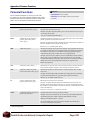
Financial Functions.............................................................................................................................................259
Date & Time Functions .......................................................................................................................................260
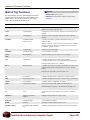
Math & Trig Functions.........................................................................................................................................262
Statistical Functions............................................................................................................................................264
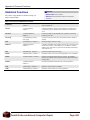
Lookup & Reference Functions ..........................................................................................................................265
Database Functions............................................................................................................................................266
Text Functions ....................................................................................................................................................267
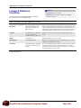
Logical Functions................................................................................................................................................268
Microsoft Office Excel 2007 Review ..................................................................................................................269
DoubleTechs.com Remote Computer Repair
Page 6
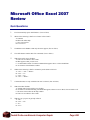
The
Fundamentals
Starting Excel 2007............................................ 11
Windows XP ............................................ 11
Windows Vista ......................................... 11
What’s New in Excel 2007................................. 12
Understanding the Excel Program Screen ..... 13
Understanding the Ribbon ............................... 14
Tabs ......................................................... 14
Groups ..................................................... 14
Buttons..................................................... 14
Using the Office Button and Quick Access
Toolbar................................................................ 15
Using Keyboard Commands ............................ 16
Keystroke shortcuts ................................. 16
Key Tips ................................................... 16
Using Contextual Menus and the Mini Toolbar
............................................................................. 17
Using Help .......................................................... 18
Search for help ........................................ 18
Browse for help........................................ 18
Choose the Help source .......................... 18
1
Microsoft Excel is a powerful spreadsheet
program that allows you to make quick
and accurate numerical calculations and
helps you to make your data look sharp
and professional. The uses for Excel are
limitless: businesses use Excel for
creating financial reports, scientists use
Excel for statistical analysis, and families
use Excel to help manage their investment
portfolios.
For 2007, Excel has undergone a major
redesign. If you’ve used Excel before,
you’ll still be familiar with much of the
program’s functionality, but you’ll notice
a completely new user interface and many
new features that have been added to
make using Excel more efficient.
This chapter is an introduction to working
with Excel. You’ll learn about the main
parts of the program screen, how to give
commands, use help, and about new
features in Excel 2007.
Exiting Excel 2007 ............................................. 20
DoubleTechs.com Remote Computer Repair
Page 10
The Fundamentals
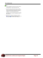
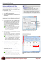
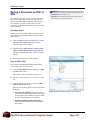
Starting Excel 2007
In order to use a program, you must start—or launch—it
first.
Exercise
• Exercise File: None required.
• Exercise: Review the new features in Microsoft Office
Excel 2007.
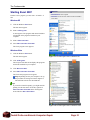
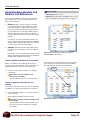
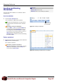
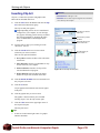
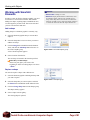
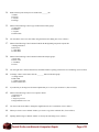
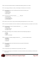
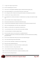
Windows XP
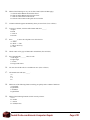
1. Click the Windows Start button.
The Start menu appears.
2. Point to All Programs.
A menu appears. The programs and menus listed here
will depend on the programs installed on your
computer.
3. Point to Microsoft Office.
4. Select Microsoft Office Excel 2007.
The Excel program screen appears.
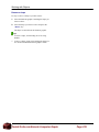
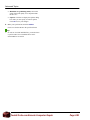
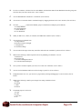
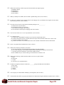
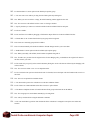
Windows Vista
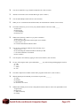
1. Click the Windows Start button.
The Start menu appears.
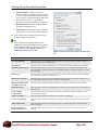
Figure 1-1: The All Programs menu in Windows XP.
2. Click All Programs.
The left pane of the Start menu displays the programs
and menus installed on your computer.
3. Click Microsoft Office.
4. Select Microsoft Office Excel 2007.
The Excel 2007 program screen appears.
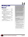
Trap: Depending on how your computer is set up,
the procedure for starting Excel 2007 might be a
little different from the one described here.
Tips
If you use Excel 2007 frequently, you might consider
pinning it to the Start menu. To do this, right-click
Microsoft Office Excel 2007 in the All Programs
menu and select Pin to Start Menu.
Figure 1-2: The All Programs menu in Windows Vista.
DoubleTechs.com Remote Computer Repair
Page 11
The Fundamentals
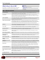
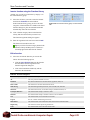
What’s New in Excel 2007
Excel 2007 is very different from previous versions. The
table below gives you an overview of what to expect.
Exercise
• Exercise File: None required.
• Exercise: Review the new features in Microsoft Office
Excel 2007.
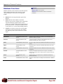
Table 1-1: What’s New in Excel 2007
New user interface
The new results-oriented user interface (UI) is the most noticeable change in Excel 2007. Traditional
menus and toolbars have been replaced by the Ribbon, a single mechanism that makes all the
commands needed to perform a task readily available.
Live Preview
Allows you to preview how a formatting change will look before applying it. Simply point to the
selection on the Ribbon or Mini Toolbar and Excel 2007 shows you a preview of what your worksheet
would look like if the selected changes were applied.
XML compatibility
The new Excel XML format ( xlsx) is much smaller in file size and makes it easier to recover damaged
or corrupted files. Files based on XML have the potential to be more robust and integrated with
information systems and external data.
Improved styles and themes
Predefined styles and themes let you change the overall look and feel of a worksheet in just a few
clicks. With Office themes, you can apply predefined formatting to workbooks and then share them
with Word and PowerPoint to give your Office documents a unified look. You can even create your own
corporate theme. Styles can be used to format specific items in Excel, such as tables and charts.
SmartArt
The new SmartArt graphics feature offers new diagram types and more layout options, and lets you
convert text such as a bulleted list into a diagram.
Save as PDF
Now you can install an Excel add-in that allows you to save a workbook as a PDF without using thirdparty software. PDF format allows you to share your worksheet with users on any platform.
Document Inspector
Removes comments, tracked changes, metadata (document history such as the author and editors) and
other information that you don’t want to appear in the finished worksheet.
Digital Signature
Adding a digital signature to a workbook prevents inadvertent changes, ensuring that your content
cannot be altered.
Better sharing capabilities
Microsoft Office SharePoint Server 2007 makes it easier to share and manage worksheets from within
Excel.
Better conditional
formatting
Conditional formatting allows you to analyze Excel data with just a few clicks. You can apply gradient
colors, data bars, and icons to cells to visually represent relationships between your data.
Easier formula writing
An expandable formula bar and Function AutoComplete are among several features that make formula
writing easier in Excel 2007.
Enhanced sorting and
filtering
Now you can sort data by color and by up to 64 levels. You can also filter by color or date, display more
than 1000 items in the AutoFilter drop-down list, filter by multiple items, and filter PivotTable data.
Improved tables (formerly
Excel lists)
Among the improvements to tables: table header rows can be turned on or off; calculated columns have
been added so you only have to enter a formula once; AutoFilter is turned on by default; and structured
references allow you to use table column header names in formulas in place of cell references.
Better charts
Visual chart element pickers allow you to quickly edit chart elements such as titles and legends,
OfficeArt allows you to format shapes with modern-looking 3-D effects, and clearer lines and charts
make charts easier to read. In addition, sharing charts with other Office programs is easier than ever,
because Word and PowerPoint now share Excel’s chart features.
New PivotTable interface
With the new PivotTable user interface, dragging data to drop zones has been replaced by clicking the
fields you want to see. You can now undo PivotTable actions, expand or collapse parts of the PivotTable
with plus and minus drill-down indicators, and sort and filter data using simple buttons.
Easier connection to external
data
Quicklaunch allows you to select from a list of data sources that your administrator has made available,
instead of having to know the server or database names, and a connection manager allows you to view
all the connections in a workbook.
New Page Layout view
With a new Page Layout view, you can see how your worksheet will look in a printed format while you
work.
DoubleTechs.com Remote Computer Repair
Page 12
The Fundamentals
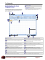
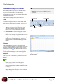
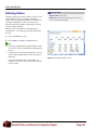
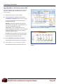
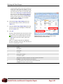
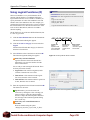
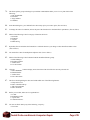
Understanding the Excel
Program Screen
The Excel 2007 program screen may seem confusing and
overwhelming at first. This lesson will help you become
familiar with the Excel 2007 program screen as well as
the new user interface.
Exercise Notes
• Exercise File: None required.
• Exercise: Understand and experiment with the different
parts of the Microsoft Office Excel 2007 screen.
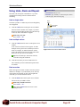
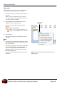
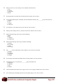
Office Button: Replaces the File menu found in previous
versions of Excel.
View buttons: Use these buttons to quickly switch between
Normal, Page Layout, and Page Break Preview views.
Quick Access Toolbar: Contains common commands such
as Save and Undo. You can add more commands as well.
Worksheet tabs: Workbooks have three worksheets by
default. You can move from one worksheet to another by
clicking the worksheet tabs.
Title bar: Displays the name of the workbook you are
working on and the name of the program you are using.
Status bar: Displays messages and feedback on the current
state of Excel. Right-click the status bar to configure it.
Close button: Click the close button in the Title bar to exit
the Excel program entirely, or click the close button in the
Ribbon to close only the current workbook.
Name box: Displays the active cell address or object name.
Click the list arrow to enter formulas.
Ribbon: The tabs and groups on the Ribbon replace the
menus and toolbars found in previous versions of Excel.
Row and column headings: Cells are organized and
referenced by row and column headings (for example, cell
A1).
Scroll bars: Use the vertical and horizontal scroll bars to
view different parts of the worksheet.
Active cell: You can enter or edit data in the active cell.
Zoom slider: Click and drag the slider to zoom in or out of a
window. You can also use the + and – buttons.
Formula Bar: Allows you to view, enter, and edit data in the
active cell. Displays values or formulas in the cell.
DoubleTechs.com Remote Computer Repair
Page 13
The Fundamentals
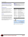
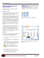
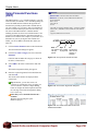
Understanding the Ribbon
Excel 2007 provides easy access to commands through
the Ribbon, which replaces the menus and toolbars found
in previous versions of Excel. The Ribbon keeps
commands visible while you work instead of hiding them
under menus or toolbars.
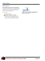
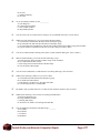
The Ribbon is made up of three basic components:
Exercise
• Exercise File: None required.
• Exercise: Click each tab on the Ribbon to view its
commands.
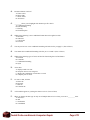
Command tab
Contextual tab
Tabs
Commands are organized into tabs on the Ribbon. Each
tab contains a different set of commands. There are three
different types of tabs:
• Command tabs: These tabs appear by default
whenever you open the Excel program. In Excel
2007, the Home, Insert, Page Layout, Formulas,
Data, Review, and View tabs appear by default.
Button
Group
Dialog Box
Launcher
Figure 1-3: Ribbon elements.
• Contextual tabs: Contextual tabs appear whenever
you perform a specific task and offer commands
relative to only that task. For example, whenever you
insert a table, the Design tab appears on the Ribbon.
• Program tabs: If you switch to a different authoring
mode or view, such as Print Preview, program tabs
replace the default command tabs that appear on the
Ribbon.
Groups
The commands found on each tab are organized into
groups of related commands. For example, the Font group
contains commands used for formatting fonts. Click the
Dialog Box Launcher ( ) in the bottom-right corner of a
group to display even more commands. Some groups also
contain galleries that display several formatting options.
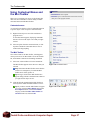
Buttons
Figure 1-4: Hiding the Ribbon gives you more room in the
program window.
One way to issue a command is by clicking its button on
the Ribbon. Buttons are the smallest element of the
Ribbon.
Tips
You can hide the Ribbon so that only tab names
appear, giving you more room in the program
window. To do this, double-click the currently
displayed command tab. To display the Ribbon again,
click any tab.
Based on the size of the program window, Excel
changes the appearance and layout of the commands
within the groups.
DoubleTechs.com Remote Computer Repair
Page 14
The Fundamentals
Using the Office Button and
Quick Access Toolbar
Near the Ribbon at the top of the program window are
two other tools you can use to give commands in Excel
2007: The Office Button and the Quick Access Toolbar.
Exercise
• Exercise File: None required.
• Exercise: Click the Office Button to open it. Move the
Quick Access Toolbar below the Ribbon, then move it back
above the Ribbon.
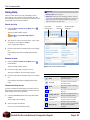
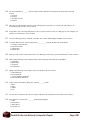
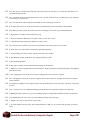
Office Button
The Office Button appears in the upper-left corner of the
program window and contains basic file management
commands including New, which creates a new file;
Open, which opens a file; Save, which saves the currently
opened file; and Close, which closes the currently opened
file.
Tips
The Office Button replaces the File menu found in
previous versions of Excel.
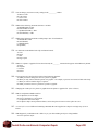
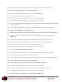
Quick Access Toolbar
The Quick Access Toolbar appears to the right of the
Office Button and provides easy access to the commands
you use most frequently. By default, the Save, Undo and
Redo buttons appear on the toolbar; however, you can
customize this toolbar to meet your needs by adding or
removing buttons.
1. Click the Customize Quick Access Toolbar button
at the end of the Quick Access Toolbar.
A list of commands you can add to the Quick Access
Toolbar appears.
Figure 1-5: The Office Button menu.
2. Select the commands you want to add or remove.
The commands are added as buttons on the Quick
Access Toolbar.
Tips
You can change where the Quick Access Toolbar
appears in the program window. To do this, click the
Customize Quick Access Toolbar button at the end
of the Quick Access Toolbar. Select Show Below the
Ribbon or Show Above the Ribbon, depending on
the toolbar’s current location.
Save
Undo
Redo
Customize
Figure 1-6: The Quick Access Toolbar.
DoubleTechs.com Remote Computer Repair
Page 15
The Fundamentals
Using Keyboard Commands
Another way to give commands in Excel 2007 is using the
keyboard. There are two different types of keyboard
commands in Excel 2007: keystroke shortcuts and Key
Tips.
Exercise
• Exercise File: None required.
• Exercise: Memorize some common keystroke shortcuts.
Then view Key Tips in the program.
Keystroke shortcuts
Without a doubt, keystroke shortcuts are the fastest way to
give commands in Excel 2007. They’re especially great
for issuing common commands, such as saving a
workbook.
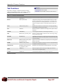
Table 1-2: Common Keystroke Shortcuts
In order to issue a command using a keystroke shortcut,
you simply press a combination of keys on your
keyboard. For example, rather than clicking the Copy
button on the Ribbon to copy a cell, you could press and
hold the copy keystroke shortcut, <Ctrl> + <C>.
Key Tips
New in Excel 2007, Key Tips appear whenever you press
the <Alt> key. You can use Key Tips to perform just about
any action in Excel, without ever having to use the mouse.
To issue a command using a Key Tip, first press the <Alt>
key. Tiny letters and numbers, called badges, appear on
the Office Button, the Quick Access Toolbar, and all of
the tabs on the Ribbon. Depending on the tab or command
you want to select, press the letter or number key
indicated on the badge. Repeat this step as necessary until
the desired command has been issued.
<Ctrl> + <O>
Opens a workbook.
<Ctrl> + <N>
Creates a new workbook.
<Ctrl> + <S>
Saves the current workbook.
<Ctrl> + <P>
Prints the worksheet.
<Ctrl> + <B>
Toggles bold font formatting.
<Ctrl> + <I>
Toggles italic font formatting.
<Ctrl> + <C>
Copies the selected cell, text or object.
<Ctrl> + <X>
Cuts the selected cell, text or object.
<Ctrl> + <V>
Pastes the selected cell, text or object.
<Ctrl> + <Home>
Moves the cell pointer to the beginning
of the worksheet.
<Ctrl> + <End>
Moves the cell pointer to the end of the
worksheet.
Key Tip badge
Figure 1-7: Press the <Alt> key to display Key Tips.
DoubleTechs.com Remote Computer Repair
Page 16
The Fundamentals
Using Contextual Menus and
the Mini Toolbar
There are two tools that you can use in Excel 2007 that
make relevant commands even more readily available:
contextual menus and the Mini Toolbar.
Exercise
• Exercise File: None required.
• Exercise: Open a contextual menu in the main area and
other parts of the program window.
Contextual menus
A contextual menu displays a list of commands related to
a specific object or area. To open a contextual menu:
1. Right-click an object or area of the worksheet or
program screen.
A contextual menu appears, displaying commands
that are relevant to the object or area that you rightclicked.
2. Select an option from the contextual menu, or click
anywhere outside the contextual menu to close it
without selecting anything.
The Mini Toolbar
New in Excel 2007 is the Mini Toolbar, which appears
when you select text or data within a cell or the formula
bar, and contains common text formatting commands.
1. Select text or data within a cell or the formula bar.
The Mini Toolbar appears above the text or data you
selected.
Figure 1-8: A contextual menu.
Trap: Sometimes the Mini Toolbar can be hard to
see due to its transparency. To make the Mini
Toolbar more visible, point to it.
Tip: A larger version of the Mini Toolbar also
appears along with the contextual menu whenever
you right-click an object or area.
2. Click the desired command on the Mini Toolbar or
click anywhere outside the Mini Toolbar to close it.
Tip: If you don’t want the Mini Toolbar to appear
every time, click the Office Button and click the
Excel Options button. Click the Personalize
category, uncheck the Show Mini Toolbar on
selection check box, and click OK.
Figure 1-9: The Mini Toolbar.
DoubleTechs.com Remote Computer Repair
Page 17
The Fundamentals
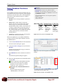
Using Help
When you don’t know how to do something in Excel
2007, look up your question in the Excel Help files. The
Excel Help files can answer your questions, offer tips, and
provide help for all of Excel’s features.
Exercise
• Exercise File: None required.
• Exercise: Search the term “formatting numbers”. Browse
topics in the “Worksheet and Excel table basics” category of
Help. Search the term “formatting numbers” again using
help files from this computer only.
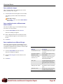
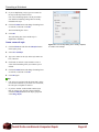
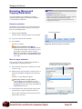
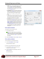
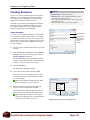
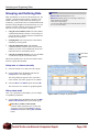
Search for help
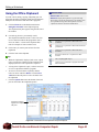
1. Click the Microsoft Office Excel Help button ( )
on the Ribbon.
Enter search
keywords here.
Choose a
help source.
Browse help topic
categories.
The Excel Help window appears.
Other Ways to Open the Help window:
Press <F1>.
2. Type what you want to search for in the “Type words
to search for” box and press <Enter>.
A list of help topics appears.
3. Click the topic that best matches what you’re looking
for.
Excel displays information regarding the selected
topic.
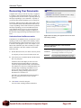
Browse for help
1. Click the Microsoft Office Excel Help button ( )
on the Ribbon.
The Excel Help window appears.
Figure 1-10: The Excel Help window.
2. Click the category that you want to browse.
The topics within the selected category appear.
3. Click the topic that best matches what you’re looking
for.
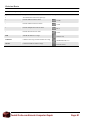
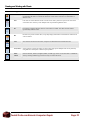
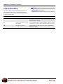
Table 1-3: Help buttons
Back
Click here to move back to the
previous help topic.
Forward
Click here to move forward to
the next help topic.
Choose the Help source
Home
If you are connected to the Internet, Excel 2007 retrieves
help from the Office Online database by default. You can
easily change this to meet your needs.
Click here to return to the Help
home page.
Print
Click here to print the current
help topic.
Change Font Size
Click here to change the size of
the text in the Help window.
Show Table of
Contents
Click here to browse for help
using the Table of Contents.
Keep On Top
Click here to layer the Help
window so that it appears behind
all other Microsoft Office
programs.
Excel displays information regarding the selected
topic.
1. Click the Search button list arrow in the Excel Help
window.
A list of help sources appears.
2. Select an option from the list.
Now you can search from that source.
DoubleTechs.com Remote Computer Repair
Page 18
The Fundamentals
Tips
When a standard search returns too many results, try
searching offline to narrow things down a bit.
Office 2007 offers enhanced ScreenTips for many
buttons on the Ribbon. You can use these ScreenTips
to learn more about what a button does and, where
available, view a keystroke shortcut for the
command. If you see the message “Press F1 for more
help”, press <F1> to get more information relative to
that command.
When you are working in a dialog box, click the
Help button ( ) in the upper right-hand corner to get
help regarding the commands in the dialog box.
DoubleTechs.com Remote Computer Repair
Page 19
The Fundamentals
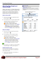
Exiting Excel 2007
When you’re finished using Excel 2007, you should exit
it. Exiting a program closes it until you need to use it
again.
Exercise
• Exercise File: None required.
• Exercise: Exit the Microsoft Office Excel 2007 program.
1. Click the Office Button.
2. Click the Exit Excel button.
The Excel program closes.
Other Ways to Exit Excel:
If there is only one Excel program window open,
click the Close button in the title bar.
Tips
Having too many programs open at a time could slow
down your computer, so it’s a good idea to exit all
programs that aren’t being used.
Exit Excel
Close the current
workbook
Figure 1-11: Two ways to Exit Excel.
DoubleTechs.com Remote Computer Repair
Page 20
Wor ksheet
Basics
Creating a New Workbook ................................ 22
Create a new blank workbook ................. 22
Create a workbook from a template ........ 22
Opening a Workbook ........................................ 23
Navigating a Worksheet.................................... 24
2
This chapter will introduce you to Excel
basics—what you need to know to create,
print, and save a worksheet.
We don’t get into great depth here, but we
make sure you understand key Excel
functionality, such as entering data and
the basics of using formulas. This chapter
will help you build a solid foundation of
Excel knowledge.
Entering Labels.................................................. 25
Entering Values.................................................. 26
Selecting a Cell Range ...................................... 27
Overview of Formulas and Using AutoSum ... 28
Entering Formulas............................................. 29
Using AutoFill .................................................... 31
Understanding Absolute and Relative Cell
References ......................................................... 32
Create a relative cell reference in a formula
................................................................. 32
Create an absolute cell reference in a
formula..................................................... 32
Using Undo, Redo and Repeat ......................... 33
Undo a single action ................................ 33
Undo multiple actions .............................. 33
Redo an action......................................... 33
Repeat an action...................................... 34
Saving a Workbook ........................................... 35
Save a new workbook ............................. 35
Save workbook changes ......................... 36
Save a workbook under a different name
and/or location ......................................... 36
Save a workbook as a different file type.. 36
Using Exercise Files
This chapter suggests exercises to practice
the topic of each lesson. There are two
ways you may follow along with the
exercise files:
• Open the exercise file for a lesson,
perform the lesson exercise, and close
the exercise file.
• Open the exercise file for a lesson,
perform the lesson exercise, and keep
the file open to perform the remaining
lesson exercises for the chapter.
The exercises are written so that you may
“build upon them”, meaning the exercises
in a chapter can be performed in
succession from the first lesson to the last.
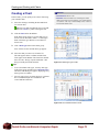
Previewing and Printing a Worksheet ............. 37
Preview a worksheet ............................... 37
Quick Print a worksheet........................... 37
Print a worksheet ..................................... 37
Closing a Workbook.......................................... 38
DoubleTechs.com Remote Computer Repair
Page 21
Worksheet Basics
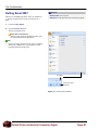
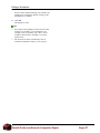
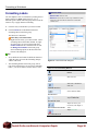
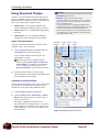
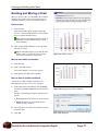
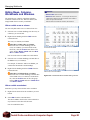
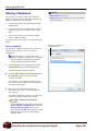
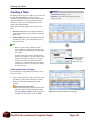
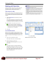
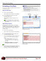
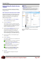
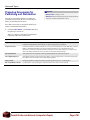
Creating a New Workbook
Creating a new workbook is one of the most basic
commands you need to know in Excel. A new workbook
automatically appears upon starting Excel, but it’s also
helpful to know how to create a new workbook within the
application. You can create a blank new workbook, such
as the one that appears when you open Excel, or you can
create a new workbook based on a template.
Exercise
• Exercise File: None required.
• Exercise: Create a new blank workbook. Then create a
new workbook from a Microsoft Office Online template.
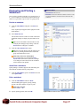
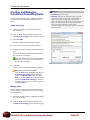
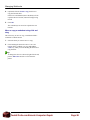
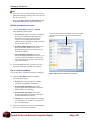
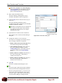
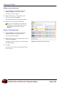
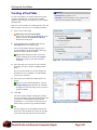
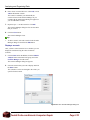
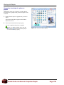
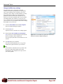
Create a new blank workbook
1. Click the Office Button and select New.
The New Workbook dialog box appears. By default,
the Blank Workbook option is already selected.
2. Make sure the Blank Workbook option is selected
and click Create.
The new blank workbook appears in the Excel
application screen.
Other Ways to Create a Blank Workbook:
Double-click the Blank Workbook option. Or
press <Ctrl> + <N>.
Figure 2-1: The New Workbook dialog box.
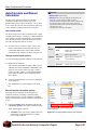
Create a workbook from a template
1. Click the Office Button and select New.
The New Workbook dialog box appears. There are
several ways you can create a new workbook from a
template. Different categories are listed to the left:
• Blank and recent: This category is selected by
default. Select a template in the Recently Used
Templates area and click Create.
• Installed Templates: Click this category to view
templates that were installed on your computer
with Microsoft Office. Select the template from
which you want to create a new workbook and
click Create.
• My templates: Select My Templates to open a
dialog box that displays templates you have
created and saved on your computer.
• New from existing: Select New from Existing to
open a dialog box that allows you to browse for a
workbook on your computer that you want to base
a new workbook on. This is essentially like
creating a copy of an existing file.
• Microsoft Office Online: Click a category to
view templates that you can download from
Office Online. Find the template you want to
download and click Download.
DoubleTechs.com Remote Computer Repair
Page 22
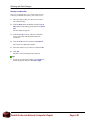
Worksheet Basics
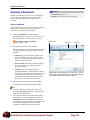
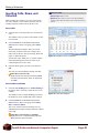
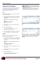
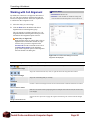
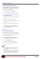
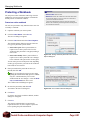
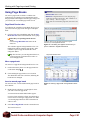
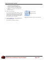
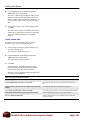
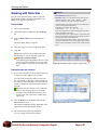
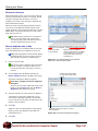
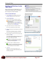
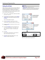
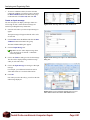
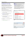
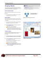
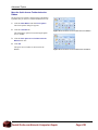
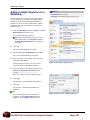
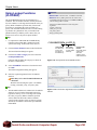
Opening a Workbook
Opening a workbook lets you work on a workbook that
you or someone else has previously created and then
saved. This lesson explains how to open a saved
workbook.
Exercise
• Exercise File: Sales2-1 xlsx
• Exercise: Open a previously-saved workbook.
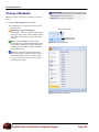
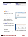
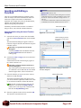
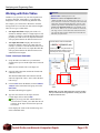
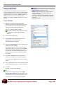
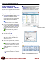
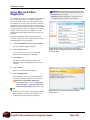
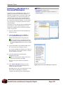
Open a workbook
You can locate an Excel file on your computer and simply
double-click it to open it, but you can also open a
workbook from within the Excel program.
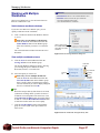
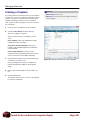
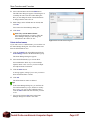
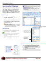
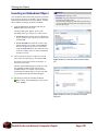
1. Click the Office Button and select Open.
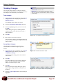
The Open dialog box appears. Next, you have to tell
Excel where the file you want to open is located.
Other Ways to Open a Workbook:
Press <Ctrl> + <O>.
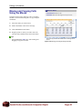
Favorite Links
Address bar
Search box
2. Navigate to the location of the saved file.
The Open dialog box has several controls that make it
easy to navigate to locations and find files on your
computer:
• Address bar: Click a link in the Address bar to
open it. Click the arrow to the right of a link to
open a list of folder within that location. Select a
folder from the list to open it.
• Favorite Links: Shortcuts to common locations
on your computer, such as the Desktop and
Documents Folder.
• Search box: This searches the contents—
including subfolders—of that window for the text
that you type. If a file’s name, file content, tags, or
other file properties match the searched text, it
will appear in the search results. Search results
appear as you enter text in the search box.
Figure 2-2: The Open dialog box. To open a file, you must
first navigate to the folder where it is saved. Most new files
are saved in the Documents folder by default.
3. Select the file you want to open and click Open.
Excel displays the file in the application window.
Tips
To open a workbook that has been used recently,
click the Office Button and select a workbook from
the Recent Documents menu.
You can pin a workbook to the Recent Documents
menu so that it is always available there. Click the
Office Button and click the Pin button next to the
workbook that you want to always be available. Click
the workbook’s Pin button again to unpin the
workbook from the Recent Documents menu.
DoubleTechs.com Remote Computer Repair
Page 23
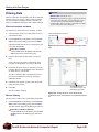
Worksheet Basics
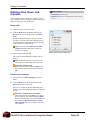
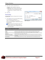
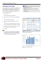
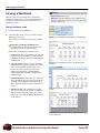
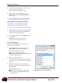
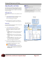
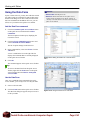
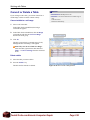
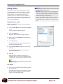
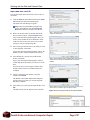
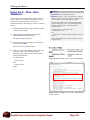
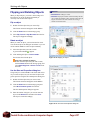
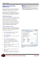
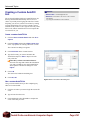
Navigating a Worksheet
Before you start entering data into a worksheet, you need
to learn how to move around in one. You must make a cell
active by selecting it before you can enter information in
it. You can make a cell active by using:
•
The Mouse: Click any cell with the white cross
pointer.
•
The Keyboard: Move the cell pointer using the
keyboard’s arrow keys.
To help you know where you are in a worksheet, Excel
displays row headings, indentified by numbers, on the left
side of the worksheet, and column headings, identified by
letters, at the top of the worksheet. Each cell in a
worksheet has its own cell address made from its column
letter and row number—such as cell A1, A2, B1, B2, etc.
You can immediately find the address of a cell by looking
at the Name Box, which shows the current cell address.
Exercise Notes
• Exercise File: Sales2-1 xlsx
• Exercise: Practice moving around in the worksheet using
both the mouse and keyboard.
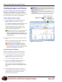
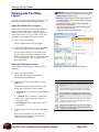
Name Box
1. Click any cell to make it active.
The cell address appears in the name box.
Figure 2-3: A cell address in the Name Box.
Now that you’re familiar with moving the cell pointer
with the mouse, try using the keyboard.
2. Press <Tab>.
The active cell is one cell to the right of the previous
cell. Refer to Table 2-1: Navigation Shortcuts for
more information on navigating shortcuts.
Tips
Excel 2007 worksheets have 1,048,576 rows and
16,384 columns! To view the off-screen portions of
the worksheet, use the horizontal and vertical scroll
bars.
To select contents within a cell, double-click the cell,
then click and drag to select the desired contents.
Using the <Ctrl> key with arrow keys is very
powerful. These key combinations jump to the edges
of data. For example, if you have a group of data in
columns A-G and another group in columns R-Z,
<Ctrl> + <→> jumps between each group of data.
Table 2-1: Navigation Shortcuts
Press
To Move
→ or <Tab>
One cell to the right.
← or
<Shift> + <Tab>
One cell to the left.
↑ or
<Shift> + <Enter>
One cell up.
↓ or <Enter>
One cell down.
<Home>
To column A in the current row.
<Ctrl> + <Home>
To the first cell (A1) in the
worksheet.
<Ctrl> + <End>
To the last cell with data in the
worksheet.
<Page Up>
Up one screen.
<Page Down>
Down one screen.
<F5> or
<Ctrl> + <G>
Opens the Go To dialog box where
you can go to a specified cell address.
DoubleTechs.com Remote Computer Repair
Page 24
Worksheet Basics
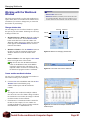
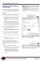
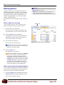
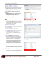
Entering Labels
Now that you’re familiar with worksheet navigation in
Excel, you’re ready to start entering data. There are two
basic types of information you can enter in a cell:
•
Labels: Any type of text or information not used in
calculations.
•
Values: Any type of numerical data: numbers,
percentages, fractions, currencies, dates, or times,
usually used in formulas or calculations.
Exercise Notes
• Exercise File: Sales2-1 xlsx
• Exercise: Type the label “Sales and Expenses” in cell A1
and the labels “Supplies”, “Office”, “Salaries”, “Utilities”,
and “Total” in the cell range A7:A11.
This lesson focuses on labels. Labels are used for
worksheet, column, and row headings. They usually
contain text, but can also consist of numerical information
not used in calculations, such as serial numbers. Excel
treats information beginning with a letter as a label and
automatically left-aligns it inside the cell.
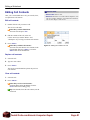
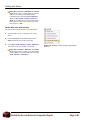
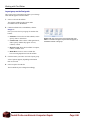
1. Click a cell where you want to add a label.
Don’t worry if the cell already contains text—
anything you type will replace the old cell contents.
2. Type the label, such as a row heading, in the cell.
3. Press the <Enter> or <Tab> key.
The cell entry is confirmed and the next cell down
becomes active.
Figure 2-4: Entering a label in a cell.
Other Ways to Confirm a Cell Entry:
Click the Enter button on the Formula Bar. Or,
press the <Tab> key.
If the label is too large to fit in the cell, the text spills
into the cell to the right, as long as that cell is empty.
If not, Excel truncates the text; it’s still there—you
just can’t see it.
Tips
Click the Cancel button on the Formula Bar to cancel
typing and return the cell to its previous state.
If you want to start a label with a number, type an
apostrophe before the number to prevent Excel from
recognizing the number as a value.
AutoComplete can help you enter labels. Enter the
first few characters of a label; Excel displays the
label if it appears previously in the column. Press
<Enter> to accept the entry or resume typing to
ignore the suggestion.
Labels that are wider than the column in which they
are entered automatically overlap the cell in the next
column over. Resize the width of the column to fix
this problem, something we’ll cover later on.
DoubleTechs.com Remote Computer Repair
Page 25
Worksheet Basics
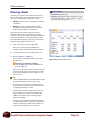
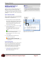
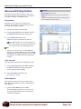
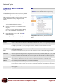
Entering Values
Now that you know how to enter labels, it’s time to work
with the other basic type of worksheet information:
values. Values are the numerical data in a worksheet that
are used in calculations. A value can be any type of
numerical information: numbers, percentages, fractions,
currencies, dates, and times.
Exercise Notes
• Exercise File: Sales2-2 xlsx
• Exercise: Enter the following values in the cell range
E7:E10: 3500, 800, 7000, 4000.
Entering values in a worksheet is no different from
entering labels—you simply type the value and confirm
the entry.
1. Click a cell and type a value.
2. Press <Enter> or <Tab> to confirm the entry.
Tips
Excel treats information that contains numbers, dates
or times as a value and automatically right-aligns it in
the cell.
Values don’t have to contain only numbers. You can
also use numerical punctuation such as a period or a
dollar sign.
Figure 2-5: Entering a value in a cell.
You can reformat dates after entering them. For
example, if you enter 4/4/07, you can easily reformat
to April 4, 2007.
DoubleTechs.com Remote Computer Repair
Page 26
Worksheet Basics
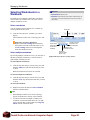
Selecting a Cell Range
To work with a range of cells, you need to know how to
select multiple cells.
1. Click the first cell you want to select in the cell range
and hold the mouse button.
Exercise Notes
• Exercise File: Sales2-3 xlsx
• Exercise: Select the cell range E7:E10.
Click to select the entire
worksheet.
2. Drag to select multiple cells.
As you drag, the selected cells are highlighted.
3. Release the mouse button.
The cell range is selected.
Other Ways to Select a Cell Range:
Press and hold the <Shift> key and use the arrow
keys to select multiple cells.
Tips
To select all the cells in a worksheet, click the Select
All button where the row and column headers come
together, or press <Ctrl> + <A>.
Figure 2-6: Selecting a range of cells with the mouse.
To select multiple non-adjacent cells, select a cell or
cell range and hold down the <Ctrl> key while you
select other cells.
DoubleTechs.com Remote Computer Repair
Page 27
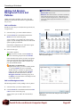
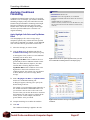
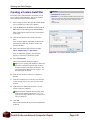
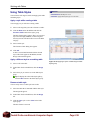
Worksheet Basics
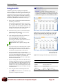
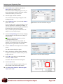
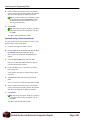
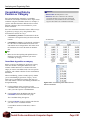
Overview of Formulas and
Using AutoSum
This lesson introduces what spreadsheet programs are
really all about: formulas.
Exercise Notes
• Exercise File: Sales2-3 xlsx.
• Exercise: AutoSum the column B expense values in cell
B11.
Formula overview
Formulas are values, but unlike regular values, formulas
contain information to perform a numerical calculation,
such as adding, subtracting, or multiplying.
All formulas must start with an equal sign (=). Then you
must specify two more types of information: the values
you want to calculate and the arithmetic operator(s) or
function name(s) you want to use to calculate the values.
Formulas can contain numbers, like 5 or 8, but more often
they reference the contents of cells. For example, the
formula =A5+A6 adds the values in cells A5 and A6.
Using these cell references is advantageous because if you
change the values in the referenced cells, the formula
result updates automatically to take the new values into
account.
Figure 2-7: The AutoSum button in the Editing group.
You’re already familiar with some of the arithmetic
operators used in Excel formulas, such as the plus sign
(+). Functions are pre-made formulas that you can use as
shortcuts or to perform calculations that are more
complicated. For example, the PMT function calculates
loan payments based on an interest rate, the length of the
loan, and the principal amount of the loan.
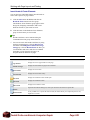
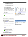
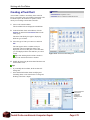
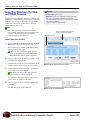
AutoSum
SUM is a common Excel function used to find the total of
a range of cells. Excel has a shortcut button, called
AutoSum, that can insert the formula for you.
1. Click a cell next to the column or row of numbers
you want to sum.
2. Click the Home tab and click the AutoSum button in
the Editing group.
The SUM function appears in the cell and a moving
dotted line appears around the cell range that Excel
thinks you want to sum. If the range is not correct,
click and drag to select the correct range.
Figure 2-8: Using the SUM function in a formula to sum a
range of cells.
Tip: Click the AutoSum button list arrow to
choose from other common functions, such as
Average.
3. Press the <Enter> key to confirm the action.
The cell range is totaled in the cell. If you change a
value in the summed range, the formula will
automatically update to show the new sum.
DoubleTechs.com Remote Computer Repair
Page 28
Worksheet Basics
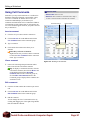
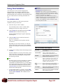
Entering Formulas
This lesson takes a look at entering formulas manually,
instead of using a shortcut like the AutoSum button.
Exercise Notes
• Exercise File: Sales2-4 xlsx.
• Exercise: Manually enter a SUM formula in cell C11 to
total the expense values in column C.
A formula starts with an equal sign, followed by:
•
Values or cell references joined by an operator.
Example: =A1+A2.
•
A function name followed by parentheses containing
function arguments.
Example: =SUM(A1:A2).
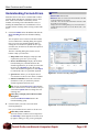
Try entering a formula yourself.
1. Click a cell where you want to enter a formula.
2. Type =, then enter the formula.
You can also enter the formula in the Formula Bar.
3. Press the <Enter> key.
The formula calculates the result and displays it in the cell
where you entered it. See Table 2-2: Examples of
Operators, References, and Formulas for examples of
common formulas in Excel.
Figure 2-9: Manually entering a formula.
Other Ways to Enter a Function:
Select the cell where you want to insert the
function. Click the Insert Function button in the
Formula Bar or click the Formulas tab on the
Ribbon and click the Insert Function button.
Select the function you want to use and click OK.
Enter the function arguments and click OK.
Adjust
horizontally
here
Expand
Formula
Bar
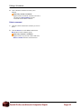
Tips
You can adjust the size of the Formula Bar. Click and
drag the rounded edge of the Name Box to adjust it
horizontally. To adjust it vertically, click and drag the
bottom border of the Formula Bar or click the
Expand Formula Bar button at the end of the Formula
Bar.
Adjust
vertically
here
Figure 2-10: Adjusting the size of the Formula bar.
You can use the Formula AutoComplete feature to
help you create and edit complex formulas. Type an =
(equal sign) in a cell or the Formula Bar and start
typing the formula. As you do this, a list appears of
functions and names that fit with the text you entered.
Select an item from the list to insert it into the
formula.
Figure 2-11: The Formula AutoComplete feature appears
as you enter a formula in the Formula bar.
DoubleTechs.com Remote Computer Repair
Page 29
Worksheet Basics
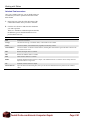
Table 2-2: Examples of Operators, References, and Formulas
Operator or Function Name
Purpose
=
All formulas must start with an equal sign.
+
Performs addition between values.
-
Performs subtraction between values.
*
Performs multiplication between values.
/
Performs division between values.
SUM
Adds all the numbers in a range.
AVERAGE
Calculates the average of all the numbers in a range.
COUNT
Counts the number of items in a range.
Example
DoubleTechs.com Remote Computer Repair
=A1+B1
=A1-B1
=B1*2
=A1/C2
=SUM(A1:A3)
=AVERAGE(A2,B1,C3)
=COUNT(A2:C3)
Page 30
Worksheet Basics
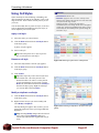
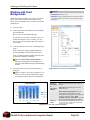
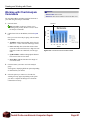
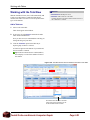
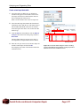
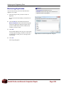
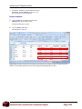
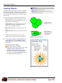
Using AutoFill
AutoFill is a great way to quickly enter sequential
numbers, months or days. AutoFill looks at cells that you
have already filled in and makes a guess about how you
would want to fill in the rest of the series. For example,
imagine you’re entering all twelve months as labels in a
worksheet. With AutoFill, you only have to enter January
and February and AutoFill will enter the rest for you.
Exercise Notes
• Exercise File: Sales2-5 xlsx.
• Exercise: Use AutoFill to fill in the months in row 3.
Labels should start with Jan in column B and end with June
in column G. Use AutoFill to copy cell range E7:E10 over to
column F, then copy cell C11 over to columns D, E, and F.
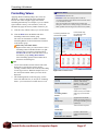
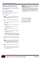
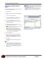
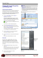
1. Select a cell or cell range that contains the data and
increment you want to use.
Excel can detect patterns pretty easily. A series of 1,
2, 3, 4 is easy to detect, as is 5, 10, 15, 20. It can also
detect a pattern with mixed numbers and letters, such
as UPV-3592, UPV-3593, UPV-3594. See Table 2-3:
Examples of AutoFill for more information.
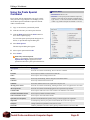
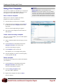
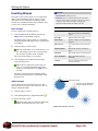
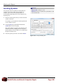
2. Position the mouse pointer over the fill handle (the
tiny box in the cell’s lower-right corner) until the
pointer changes to a plus sign .
3. Click and drag the fill handle to the cells that you
want to AutoFill with the information.
Figure 2-12: In this example, AutoFill fills in months after
January into the selected cells. Notice that a screen tip
appears to show the content being filled into the cells.
As you click and drag, a screen tip appears
previewing the value that will be entered in the cell
once you release the mouse button.
Tip: AutoFill is also a quick way to copy cells.
Tips
If you select only one cell, that same value is copied
to the adjacent cells when you AutoFill—unless
Excel recognizes it as a date or time, in which case it
will fill in the next logical date or time period.
If you use AutoFill to copy a cell containing a
formula with a cell reference, such as =A3, the filled
cells will contain updated formulas that are relative to
their location. For example, if you AutoFill the
formula =A3 from cell D5 to cell E5, cell E5 will be
filled with the formula =B3.
If you’re working with a data series that increases by
increments other than one (such as every-other day or
every-other month), select the cells that show Excel
the increment to use when filling the data series. For
example, if you enter 3 and 5 in adjacent cells, select
both cells and AutoFill the next cell; Excel will enter
7 in that next cell.
After using AutoFill the AutoFill Options button
In this example, AutoFill
copies the formula from
C11 into the other cells.
Figure 2-13: Copying a formula using the AutoFill feature.
Table 2-3: Examples of AutoFill
Selected Cell(s)
AutoFill Entries in Next Three Cells
January
February, March, April
5:00
6:00, 7:00, 8:00
Quarter 1
Quarter 2, Quarter 3, Quarter 4
5
10
15
20
25
Click this button to view different ways
appears.
to perform or complete the AutoFill.
DoubleTechs.com Remote Computer Repair
Page 31
Worksheet Basics
Understanding Absolute and
Relative Cell References
A cell reference identifies a cell or cell range and tells
Excel which values to use in a formula. There are two
types of cell references.
•
Exercise Notes
• Exercise File: Sales 2-6 xlsx.
• Exercise: Enter the formula =F7*$G$2 in cell G7. Copy
cell G7 to cells G8:G10. Copy cell F11 over to cell G11.
Relative: Relative references (like A1) tell Excel
how to find another cell starting from the cell that
contains the formula. Using a relative reference is
like giving someone directions that explain where to
go from where they are currently standing. When a
formula containing relative references is moved, it
will reference new cells based on their location to the
formula.
For example, if cell A2 contained the formula =A1,
and you copied and pasted the formula to cell B2, the
formula in B2 would read =B1 because the reference
is relative to the location of the formula.
•
Absolute: Absolute references (like $A$1) always
refer to the same cell address, even if the formula is
moved.
For example, if cell A2 contained the formula =$A$1,
and you copied and pasted the formula to cell B2, the
formula in B2 would still read =$A$1.
Figure 2-14: A formula with a relative (F7) and an
absolute ($G$2) cell reference.
Create a relative cell reference in a formula
Relative cell addresses are usually the desired way to
reference other cells in formulas, which is why they are
the default method used by Excel to reference cells.
Here the formula from the previous figure has been filled down.
The F7 reference has changed to F8 because it was relative,
while $G$2 stayed the same because it was absolute.
1. Click the cell you want to reference, for example
click cell B4.
Other Ways to Create a Relative Cell
Reference in a Formula:
Type the address of the cell, for example type B4.
Create an absolute cell reference in a
formula
If you want a cell reference to always refer to a particular
cell address, you need to use an absolute cell reference.
1. Press and hold the <F4> key as you click the cell you
want to reference.
Dollar signs $ are added to the cell reference.
Other Ways to Add an Absolute Cell Reference
in a Formula:
Type the address of the cell with $ (dollar signs)
before every reference heading. (For example,
type $B$4).
Figure 2-15: Relative vs. absolute cell references.
DoubleTechs.com Remote Computer Repair
Page 32
Worksheet Basics
Using Undo, Redo and Repeat
The undo, redo, and repeat commands are very useful
commands for working with cell contents and cell
formatting.
Exercise Notes
• Exercise File: Sales2-7 xlsx.
• Exercise: Type “Monthly” in cell A2 and press <Enter>.
Undo the typing. Then redo the typing.
Undo a single action
Undo
button
Undo does just that—it undoes any actions as though they
never happened.
Undo button
list arrow
1. Click the Undo button on the Quick Access Toolbar.
Your last action is undone. For example, if you had
deleted an item and then decided you wanted to keep
it after all, undo would make it reappear.
Other Ways to Undo:
Press <Ctrl> + <Z>.
Undo multiple actions
1. Click the Undo button list arrow on the Quick Access
Toolbar.
A list of the last actions in Excel appears. To undo
multiple actions, point to the command you want to
undo. For example, to undo the last three actions,
point at the third action in the list. Each action done
before the one you select is also undone.
Figure 2-16: The Undo and Redo buttons.
Tip: You can undo up to 100 actions in Excel,
even after saving the workbook.
2. Click the last action you want to undo in the list.
The command you select and all subsequent actions
are undone.
Redo an action
Redo is the opposite of undo: it redoes an action you have
undone. For example, if you decide that you do, after all,
want to delete an item that you have just brought back
with undo, you can redo the delete action.
1. Click the Redo button on the Quick Access Toolbar.
The last action you undid is redone.
Other Ways to Redo an Action:
Press <Ctrl> + <Y>.
Tip: Click the Redo button list arrow to redo
multiple actions.
DoubleTechs.com Remote Computer Repair
Page 33
Worksheet Basics
Repeat an action
Repeat is different from redo, because repeat applies the
last command to any selected text. For example, rather
than applying bold formatting by clicking the Bold button
repeatedly, you can repeat the bold command with the
keystroke shortcut or Repeat button.
1. Press <F4>.
The command is repeated.
Repeat button
Figure 2-17: The Repeat button on the Quick Access
Toolbar. This does not appear on the Quick Access
Toolbar by default in Excel.
Other Ways to Repeat a Command:
Add the Repeat command to the Quick Access
Toolbar. Then, click the Repeat button on the
Quick Access Toolbar to repeat the command.
DoubleTechs.com Remote Computer Repair
Page 34
Worksheet Basics
Saving a Workbook
After you’ve created a workbook, you need to save it if
you want to use it again. Also, if you make changes to a
workbook you’ll want to save it. You can even save a
copy of an existing workbook with a new name, to a
different location, or using a different file type.
Exercise Notes
• Exercise File: None required.
• Exercise: Create a new workbook and save it with the file
name “Saved Workbook.” Type your name in cell A1 and
save the workbook with a new name: “Updated Workbook”.
Save a new workbook
1. Click the Save button on the Quick Access Toolbar.
The Save As dialog box appears.
Favorite Links
Address bar
Other Ways to Save:
Press <Ctrl> + <S>. Or, click the Office Button
and select Save.
2. Specify the drive and/or folder where you want to
save your workbook.
The Save As dialog box has several controls that
make it easy to navigate to locations on your
computer:
• Address bar: Click a link in the Address bar to
open it. Click the arrow to the right of a link to
open a list of folder within that location. Select a
folder from the list to open it.
• Favorite Links: Shortcuts to common locations
on your computer, such as the Desktop and
Documents Folder.
• Folders List: View the hierarchy of drives and
folders on your computer by expanding the
Folders list.
3. Enter the file name in the File name text box.
Folders List
Figure 2-18: The Save As dialog box. New files are saved
in the Documents folder by default.
4. Click Save.
DoubleTechs.com Remote Computer Repair
Page 35
Worksheet Basics
Save workbook changes
Once you make changes to a workbook you’ve saved
before, you need to save it again.
1. Click the Save button on the Quick Access Toolbar.
Any changes you have made to the workbook are
saved.
Other Ways to Save:
Press <Ctrl> + <S>. Or, click the Office Button
and select Save.
Save a workbook under a different name
and/or location
You can save another copy of a saved document using a
new name or in a new location.
1. Click the Office Button and select Save As.
The Save As dialog box appears.
2. Enter a different name for the file in the File name
text box. And/or navigate to a new location to save
the file.
3. Click Save.
Save a workbook as a different file type
Just as some people can speak several languages, Excel
can read and write in other file formats. Saving a copy of
a workbook in a different file type makes it easier to share
information between programs.
1. Click the Office Button and select Save As.
Table 2-4: Common Excel File Formats
File Type
Description
Excel Workbook ( xlsx)
The default format for Excel 2007
workbooks.
Excel Macro-Enabled
Workbook ( xlsm)
This file format supports macros
in Excel 2007.
Excel 97- Excel 2003
Workbook ( xls)
Workbooks in this format can be
used by all versions of Excel.
Does not support XML.
PDF (.pdf)
Use this format for files you want
to share, but do not want to be
changed. Requires an Excel addin.
Web page ( htm, html)
This format is used to create Web
pages.
XML Data ( xml)
This file type is used exclusively
for XML-enabled workbooks.
The Save As dialog box appears.
2. Click the Save as type list arrow and select a file
format.
3. Click Save.
DoubleTechs.com Remote Computer Repair
Page 36
Worksheet Basics
Previewing and Printing a
Worksheet
Once you have created a worksheet, you can print copy of
it—if your computer is connected to a printer. Before you
do this, it’s a good idea to preview how it’s going to look.
Exercise Notes
• Exercise File: Sales2-8 xlsx.
• Exercise: Preview the Sales2-8 worksheet. Zoom in on the
previewed worksheet. Close the Preview mode. Print the
worksheet.
Preview a worksheet
1. Click the Office Button and point to the Print list
arrow.
A list of print options appears in the right pane of the
Office Button.
2. Select Print Preview.
The document is shown in Preview mode. Notice that
the Ribbon changes to display only the Print Preview
tab.
Tip: Use the commands on the Print Preview tab
to adjust print and page setup settings. Click the
Zoom button to enlarge the worksheet.
3. Click the Close Print Preview button.
Tip: You can print directly from the Print Preview
window by clicking the Print button in the Print
group on the Print Preview tab.
Other Ways to Preview a Worksheet:
New in Excel 2007, you can click the Page
Layout View button on the Status Bar to change
views and get a better idea of how the worksheet
will be laid out when printed.
Figure 2-19: A list of print options.
Quick Print a worksheet
Quick printing a worksheet bypasses the Print dialog box
and sends the worksheet directly to the printer.
1. Click the Office Button, point to the Print arrow and
select Quick Print.
Print a worksheet
1. Click the Office Button and select Print.
The Print dialog box appears. Specify printing
options such as the number of copies to print.
Other Ways to Print:
Press <Ctrl> + <P>.
2. Specify printing options, then click OK.
Figure 2-20: A worksheet shown in print preview.
DoubleTechs.com Remote Computer Repair
Page 37
Worksheet Basics
Closing a Workbook
When you’re done working on a workbook, you need to
close it.
Exercise Notes
• Exercise File: Any open workbook.
• Exercise: Close all open workbooks.
1. Click the Office Button and select Close.
The workbook closes. You can access the file again
by opening it later.
Exit the Excel program.
Other Ways to Close a Workbook:
Press <Ctrl> + <W>. Or, click the Close button
in the upper right corner of the workbook window
(not the one even farther up in the corner in the
title bar).
Tip: If you have multiple workbooks open,
clicking the active workbook’s Close button only
closes that one workbook. The other workbooks
remain open in the window until you click their
close buttons as well.
Close the active
workbook window.
Figure 2-21: The Close button.
Trap: The close button located in the title bar
closes only the active workbook if there is more
than workbook open. However, if there is only
one open, it closes it and causes you to exit the
Excel program entirely.
Figure 2-22: Closing a workbook.
DoubleTechs.com Remote Computer Repair
Page 38
Editing a
Wor ksheet
Editing Cell Contents ........................................ 40
Edit cell contents...................................... 40
Replace cell contents............................... 40
Clear cell contents ................................... 40
3
This chapter will show you how to edit
your Excel worksheets. You’ll learn how
to edit cell contents; cut, copy and paste
information; insert and delete columns
and rows; undo any mistakes you might
make; and even correct your spelling
errors.
Cutting, Copying, and Pasting Cells ............... 41
Moving and Copying Cells Using the Mouse.. 43
Using the Office Clipboard ............................... 44
Using the Paste Special Command ................. 45
Checking Your Spelling..................................... 46
Inserting Cells, Rows, and Columns ............... 48
Deleting Cells, Rows, and Columns ................ 49
Using Find and Replace.................................... 50
Search options......................................... 51
Using Cell Comments ....................................... 52
Insert a comment ..................................... 52
View a comment ...................................... 52
Edit a comment........................................ 52
Delete a comment.................................... 53
Tracking Changes.............................................. 54
Track changes ......................................... 54
Accept/reject changes ............................. 54
DoubleTechs.com Remote Computer Repair
Using Exercise Files
This chapter suggests exercises to practice
the topic of each lesson. There are two
ways you may follow along with the
exercise files:
• Open the exercise file for a lesson,
perform the lesson exercise, and close
the exercise file.
• Open the exercise file for a lesson,
perform the lesson exercise, and keep
the file open to perform the remaining
lesson exercises for the chapter.
The exercises are written so that you may
“build upon them”, meaning the exercises
in a chapter can be performed in
succession from the first lesson to the last.
Page 39
Editing a Worksheet
Editing Cell Contents
Once you’ve entered data into a cell, you can edit, clear,
or replace those cell contents.
Edit cell contents
Exercise Notes
• Exercise File: Sales3-1 xlsx
• Exercise: Edit cell A1 so it reads “Sales & Expenses,” and
cell A6 so it reads “Total Exp.,” then replace the contents of
cell A9 with “Wages”. Clear cell A2.
1. Double-click the cell you want to edit.
The cell is in edit mode.
Other Ways to Enter Edit Mode:
Select the cell and press <F2>.
2. Edit the contents of the cell, in the cell.
Use the arrow keys and the <Delete> and
<Backspace> keys to help you edit the cell contents.
3. Press <Enter>.
Other Ways to Edit Cell Contents:
Select the cell, then edit the cell’s contents in the
Formula Bar and. Press <Enter> or click the
Enter button on the Formula bar.
Figure 3-1: Editing the contents of a cell.
Replace cell contents
1. Select the cell.
2. Type new text or data.
3. Press <Enter>.
The newly typed information replaces the previous
cell contents.
Clear cell contents
1. Select the cell.
2. Press <Delete>.
Other Ways to Clear Cell Contents:
Under the Home tab on the Ribbon, click the
Clear button in the Editing group.
Tip: Note that this clears the cell contents, not the
actual cell.
DoubleTechs.com Remote Computer Repair
Page 40
Editing a Worksheet
Cutting, Copying, and Pasting
Cells
You can move information around in an Excel worksheet
by cutting or copying and then pasting the cell data in a
new place. You can work with one cell at a time or ranges
of cells.
Exercise Notes
• Exercise File: Sales3-2 xlsx
• Exercise: Copy cell A11 and paste it in cell A13. Then cut
cell A6 and paste it over the contents in cell A11.
Tips
You may cut, copy, and paste any item in a
worksheet, such as clip art or a picture, in addition to
cell data.
A moving dashed border
appears around a cell or cell
range when you cut or copy it.
Copy cells
When you copy a cell, the selected cell data remains in its
original location and is added to the Clipboard.
The Paste Options
Smart Tag appears
after pasting. Click
this button to specify
how information is
pasted into your
worksheet.
1. Select the cell(s) you want to copy.
Tip: If you want to cut or copy only selected parts
of a cell’s contents, double-click the cell to
display a cursor and select the characters you
want to cut.
Figure 3-2: Copying and pasting a cell.
2. Click the Home tab on the Ribbon and click the
Copy button in the Clipboard group.
Other Ways to Copy Cells:
Press <Ctrl> + <C>. Or, right-click the selection
and select Copy from the contextual menu.
Cut cells
When you cut a cell, it is removed from its original
location and placed in a temporary storage area called the
Clipboard.
1. Select the cell(s) you want to cut.
2. Click the Home tab on the Ribbon and click the Cut
button in the Clipboard group.
A line of marching ants appears around the selected
cells and the message “Select destination and press
ENTER or choose Paste” appears on the status bar.
Other Ways to Cut Cells:
Press <Ctrl> + <X>. Or, right-click the selection
and select Cut from the contextual menu.
Tip: When you cut cells, you have a shortcut to
pasting them: select the destination and press
<Enter>.
DoubleTechs.com Remote Computer Repair
Page 41
Editing a Worksheet
Paste cells
After cutting or copying, select a new cell and paste the
item that you last cut or copied into the worksheet.
1. Select the cell where you want to paste the copied or
cut cell(s).
When you select a destination to paste a range of
cells you only have to designate the first cell where
you want to paste the cell range.
2. Click the Home tab on the Ribbon and click the
Paste button in the Clipboard group.
Paste Options
Smart Tag
The cut or copied cell data is pasted in the new
location.
Other Ways to Paste Cells:
Press <Ctrl> + <V>. Or, right-click where you
want to paste and select Paste from the contextual
menu.
3. Press <Enter>.
The line of marching ants around the selected cells
disappears.
Tips
After pasting, a Paste Options Smart Tag may appear.
Click this button to specify how information is pasted
into your worksheet.
You may specify what you want to paste by using the
Paste Special command. Click the Paste button list
arrow in the Clipboard group and select Paste
Special from the list. Choose a paste option in the
Paste Special dialog box.
To collect and paste multiple items, open the Office
Clipboard.
Figure 3-3: The Paste Options Smart Tag offers a list of
pasting options.
DoubleTechs.com Remote Computer Repair
Page 42
Editing a Worksheet
Moving and Copying Cells
Using the Mouse
Exercise Notes
• Exercise File: Sales3-3 xlsx
• Exercise: Move the cell range A7:G13 up one row.
Using the mouse to move and copy cells is even faster
and more convenient than using the cut, copy and paste
commands.
1. Select the cell(s) you want to move.
2. Point to the border of the cell or cell range.
3. Click and hold the mouse button.
4. Drag the pointer to where you want to move the
selected cell(s) and then release the mouse button.
Tips
Press and hold the <Ctrl> key while clicking and
dragging to copy the selection.
The screen tip previews the address of the cell range as it is
moved.
Figure 3-4: Moving a cell range using the mouse.
DoubleTechs.com Remote Computer Repair
Page 43
Editing a Worksheet
Using the Office Clipboard
If you do a lot of cutting, copying, and pasting you will
appreciate the Office Clipboard, which collects and pastes
multiple items from Excel and other Office programs.
1. Click the Home tab on the Ribbon and click the
Dialog Box Launcher in the Clipboard group.
Exercise Notes
• Exercise File: Sales3-4 xlsx
• Exercise: Display the Clipboard. Copy the cell range
B3:F3, then copy the cell range A4:A12. In cell B14, paste
the copied B3:F3 range from the Clipboard. Close the
Clipboard. Clear the contents of cells B14:F14.
The Clipboard task pane appears along the left side of
the window.
2. Cut and copy items as you normally would.
The Clipboard can hold 24 items at a time. The icon
next to each item indicates the program the item is
from. See Table 3-1: Icons in the Clipboard Task
Pane for examples of some common icons.
3. Click where you want to paste an item from the
Clipboard.
4. Click the item in the Clipboard.
Tips
While the Clipboard is displayed, each cut or copied
item is saved to the Clipboard. If the Clipboard is not
displayed, the last cut or copied item is replaced.
Table 3-1: Icons in the Clipboard Task Pane
Content cut or copied from a Microsoft Excel
workbook.
Content cut or copied from a Microsoft PowerPoint
presentation.
Content cut or copied from a Microsoft Word
document.
Web page contents cut or copied from a Web
browser.
Cut or copied graphic object.
Content cut or copied from a program other than
Microsoft Office.
As long as the Clipboard is open, it collects items that
are cut or copied from all Office programs.
To remove an item from the Clipboard, click the
item’s list arrow and select Delete. Click the Clear
All button in the task pane to remove all items from
the Clipboard.
Click the Options button near the bottom of the task
pane to control how the Clipboard operates.
Copied and cut items
appear in the Clipboard
task pane.
Figure 3-5: A worksheet with the Clipboard task pane displayed.
DoubleTechs.com Remote Computer Repair
Page 44
Editing a Worksheet
Using the Paste Special
Command
Excel’s Paste Special command lets you specify exactly
what you want to copy and paste. For example, you can
use the Paste Special command to replace the formula
with its calculated value.
Exercise Notes
• Exercise File: Sales3-5 xlsx
• Exercise: Use the paste special command to replace the
formulas in cell range G4:G9 with their calculated values.
Type “Net Inc.” in cell A12 and enter the formula =B4-B10
in B12. Copy cell B12 and paste the formula to C12:G12.
1. Copy or cut an item as you normally would.
2. Click the cell where you want to paste the item.
3. Click the Home tab and click the Paste button list
arrow in the Clipboard group.
Use one of the paste special options that appears in
the list, or open the Paste Special dialog box.
4. Select Paste Special.
The Paste Special dialog box appears.
5. Select a paste option and click OK.
6. Press <Enter>.
Other Ways to Paste Special:
Paste as you normally would. Click the Paste
Options Smart Tag that appears next to the
pasted item and select a paste option from the list.
Figure 3-6: The Paste Special dialog box.
Table 3-2: Paste Special Options
Paste Option
Description
All
Pastes all cell contents and formatting. Same as the Paste command.
Formulas
Pastes only the formulas as entered in the formula bar.
Values
Pastes only the values as displayed in the cells.
Formats
Pastes only cell formatting. Same as using the Format Painter button.
Comments
Pastes only comments attached to the cell.
Validation
Pastes data validation rules for the copied cells to the paste area.
All using Source theme
Pastes all cell contents and formatting, including the theme, if one was applied to the source data.
All except borders
Pastes all cell contents and formatting applied to the copied cell except borders.
Column widths
Pastes only the width of the source cell’s column to the destination cell’s column.
Formulas and number formats
Pastes only the formulas and number formats.
Values and number formats
Pastes only the values and number formats.
Operation (several options)
Specifies which mathematical operation, if any, you want to apply to the copied data.
Skip blanks
Avoids replacing values in your paste area when blank cells occur in the copy area.
Transpose
Changes columns of copied data to rows, and vice versa.
Paste Link
Links the pasted data to the source data by pasting a formula reference to the source data.
DoubleTechs.com Remote Computer Repair
Page 45
Editing a Worksheet
Checking Your Spelling
You can use Excel’s spell checker to find and correct
spelling errors in your worksheets. To check the spelling
of a worksheet all at once, use the Spelling dialog box.
Exercise Notes
• Exercise File: Sales3-6 xlsx
• Exercise: Run a spell check and correct spelling for the
entire worksheet.
1. Click the Review tab on the Ribbon and click the
Spelling button in the Proofing group.
Excel begins checking spelling with the active cell.
Tip: Depending on which cell is active when you
start the spell check, you may see a dialog box
that asks you if you want to start your spell check
from the beginning of the sheet. Select Yes.
Other Ways to Check Spelling:
Press <F7>.
If Excel finds an error, the Spelling dialog box
appears with the misspelling in the “Not in
Dictionary” text box. You have several options to
choose from when the Spelling dialog box opens:
• Ignore Once: Accepts the spelling and moves on
to the next spelling error.
Figure 3-7: The Spelling dialog box.
• Ignore All: Accepts the spelling and ignores all
future occurrences of the word in the worksheet.
• Add to Dictionary: If a word is not recognized in
the Microsoft Office Dictionary, it is marked as
misspelled. This command adds the word to the
dictionary so it is recognized in the future.
• Change: Changes the spelling of the word to the
spelling that is selected in the Suggestions list.
• Change All: Changes all occurrences of the word
in the worksheet to the selected spelling.
Trap: Exercise caution when using this
command—you might end up changing
something you didn’t want to change.
• AutoCorrect: Changes the spelling of the word to
the spelling that is selected in the Suggestions list,
and adds the misspelled word to the AutoCorrect
list so that Excel will automatically fix it
whenever you type it in the future.
2. If the word is spelled incorrectly, select the correct
spelling from the Suggestions list. Then click
Change, Change All, or AutoCorrect. If the word is
spelled correctly, click Ignore Once, Ignore All,
Add to Dictionary.
Excel applies the command and moves on to the next
misspelling.
DoubleTechs.com Remote Computer Repair
Page 46
Editing a Worksheet
Once Excel has finished checking your worksheet for
spelling errors, a dialog box appears, telling you the
spelling check is complete.
3. Click OK.
The dialog box closes.
Tips
Excel cannot catch spelling errors that occur because
of misuse. For example, if you entered the word
“through” when you meant to type “threw,” Excel
wouldn’t catch it because “through” is a correctly
spelled word.
The AutoCorrect feature automatically corrects
commonly misspelled words for you as you type.
DoubleTechs.com Remote Computer Repair
Page 47
Editing a Worksheet
Inserting Cells, Rows, and
Columns
While working on a worksheet, you may need to insert
new cells, columns, or rows. When you insert cells, the
existing cells shift to make room for the new cells.
Exercise Notes
• Exercise File: Sales3-7 xlsx
• Exercise: Select cell A1, insert a new cell and shift the
existing cells to the right. Insert a new row between rows 9
and 10.
Insert cells
1. Select the cell or cell range where you want to insert
cells.
The number of cells you select is the number of cells
to be inserted.
2. Click the Home tab on the Ribbon and click the
Insert list arrow in the Cells group. Select Insert
Cells.
The Insert dialog box appears. Here you can tell
Excel how you want to move the existing cells to
make room for the new ones by selecting “Shift cells
right” or “Shift cells down.”
Figure 3-8: Inserting a cell in a worksheet.
You can also select “Entire row” or “Entire column”
in the Insert dialog box to insert an entire row or
column and not just a cell or cells.
3. Select the insert option you want to use and click
OK.
The cell(s) are inserted and the existing cells shift.
Other Ways to Insert Cells:
Right-click the selected cell(s) and select Insert
from the contextual menu. Select an option and
click OK.
Insert rows or columns
1. Select the row heading below or column heading to
the right of where you want to insert the new row or
column.
The number of row or column headings you select is
the number of row or columns that will be inserted.
Figure 3-9: The Insert dialog box.
2. Click the Home tab on the Ribbon and click the
Insert list arrow in the Cells group. Select Insert
Rows or Insert Columns.
The row or column is inserted. Existing rows are
shifted downward, while existing columns are shifted
to the right.
Other Ways to Insert Rows or Columns:
Right-click a row or column heading and select
Insert from the contextual menu.
DoubleTechs.com Remote Computer Repair
Page 48
Editing a Worksheet
Deleting Cells, Rows, and
Columns
You can quickly delete existing cells, columns, or rows
from a worksheet. When you delete cells the existing cells
shift to fill the space left by the deletion.
Exercise Notes
• Exercise File: Sales3-8 xlsx
• Exercise: Delete cell A1 and shift cells to the left. Delete
row 10.
Delete cells
1. Select the cell(s) you want to delete.
2. Click the Home tab on the Ribbon and click the
Delete list arrow in the Cells group. Select Delete
Cells.
The Delete dialog box appears. Here you can tell
Excel how you want to move the remaining cells to
cover the hole left by the deleted cell(s) by selecting
“Shift cells left” or “Shift cells up.”
Tip: You can also select Entire row or Entire
column in the Delete dialog box to delete an
entire row or column.
3. Select an option and click OK.
Figure 3-10: The Delete dialog box.
The cell(s) are deleted and the remaining cells are
shifted.
Trap: Pressing the <Delete> key only clears a
cell’s contents, it doesn’t delete the actual cell.
Other Ways to Delete Cells:
Right-click the selection and select Delete from
the contextual menu. Select an option and click
OK.
Delete rows or columns
1. Select the row or column heading(s) you want to
delete.
2. Click the Home tab on the Ribbon and click the
Delete button in the Cells group.
The rows or columns are deleted. Remaining rows
are shifted up, while remaining columns are shifted to
the left.
Other Ways to Delete Rows or Columns:
Select the column or row heading(s) you want to
delete, right-click any of them, and select Delete
from the contextual menu. Or, click the Delete list
arrow and select Delete Sheet Rows or Delete
Sheet Columns. The row or column of the active
cell is deleted.
DoubleTechs.com Remote Computer Repair
Page 49
Editing a Worksheet
Using Find and Replace
Don’t waste time scanning your worksheet for labels and
values that you want to replace with something new:
Excel’s find and replace commands can do this for you
with just a few clicks of your mouse.
Exercise Notes
• Exercise File: Sales3-9 xlsx
• Exercise: Use the Replace feature to find and replace all
instances of “Sales” with “Income” in the worksheet.
Find
The Find feature makes it very easy to find specific words
and values in a worksheet.
1. Click the Home tab on the Ribbon and click the Find
& Select button in the Editing group. Select Find
from the list.
The Find tab of the Find and Replace dialog box
appears.
Other Ways to Find Text:
Press <Ctrl> + <F>.
2. Type the text or value you want to find in the “Find
what” text box.
Figure 3-11: The Find tab of the Find and Replace dialog
box.
3. Click the Find Next button.
Excel jumps to the first occurrence of the word,
phrase, or value that you entered.
4. Click the Find Next button again to move on to other
occurrences. When you’re finished, click Close.
Replace
Replace finds specific words and values, and then
replaces them with something else.
Figure 3-12: The Replace tab of the Find and Replace
dialog box.
1. Click the Home tab on the Ribbon and click the Find
& Select button in the Editing group. Select Replace
from the list.
The Replace tab of the Find and Replace dialog box
appears.
Other Ways to Replace Text:
Press <Ctrl> + <H>.
2. Type the text or value you want replace in the “Find
what” text box.
3. Type the replacement text or value in the “Replace
with” text box.
4. Click the Find Next button.
Excel jumps to the first occurrence of the word,
phrase, or value in the “Find what” box.
DoubleTechs.com Remote Computer Repair
Page 50
Editing a Worksheet
5. Choose how you want to replace the text:
• Replace: Click to replace the current item.
• Replace All: Click to replace each item found in
the document. Use this command with caution:
you might replace something you didn’t want to
replace.
6. Click Close.
Search options
Use Excel’s search options to change how Excel searches
in the document.
1. Click the More button in the Find and Replace dialog
box to specify how to search for text.
Table 3-3: Find and Replace Search Options
describes the Search Options available under the Find
and Replace tabs.
Figure 3-13: The Find and Replace dialog box with search
options displayed.
Trap: If you specify Search Options, make sure to
turn them off when you are finished. Otherwise,
subsequent find or replace commands will use the
same search options.
Table 3-3: Find and Replace Search Options
Within
Choose whether to search within just the current sheet or the entire workbook.
Search
Search by rows (left to right, then top to bottom) or columns (top to bottom, then left to right).
Look in
Specify which kinds of data you want to search in, such as formulas, values, or comments.
Match case
Searches exactly as text is typed in the text box.
Match entire cell contents
Searches only for cells that match the contents in the text box entirely. Parts of phrases or words are
not included.
Format button
Specify formatting characteristics you want to find attached to the text in the Find what text box.
DoubleTechs.com Remote Computer Repair
Page 51
Editing a Worksheet
Using Cell Comments
Sometimes you may need to add notes to a workbook to
document complicated formulas or questionable values,
or to leave a comment for another user. Excel’s cell
comments command helps you document your
worksheets and make them easier to understand. Think of
cell comments as Post-It Notes that you can attach to any
cell. Cell comments appear whenever you point at the cell
they’re attached to.
Exercise Notes
• Exercise File: Sales3-10 xlsx
• Exercise: Add a comment to cell B4 that reads “Why is
income so low this month?” Then delete the comment.
Comment text box
Resize handle
Insert a comment
1. Click the cell you want to attach a comment to.
2. Click the Review tab on the Ribbon and click the
New Comment button in the Comments group.
3. Type a comment.
4. Click outside the comment area when you’re
finished.
Other Ways to Insert a Comment:
Right-click the cell you want to attach a comment
to and select New Comment from the contextual
menu. Type a comment.
View a comment
Figure 3-14: Entering a cell comment.
1. Point to the red triangle-shaped comment marker
that’s located in the cell with the comment.
Tip: To display a comment all the time, click the
cell with the comment, then click the Review tab
on the Ribbon and click the Show/Hide
Comments button in the Comments group. Or,
click the Show All Comments button in the
Comments group to display all the comments in a
worksheet at once.
Edit a comment
1. Click the cell that contains the comment you want to
edit.
2. Click the Review tab on the Ribbon and click the
Edit Comment button in the Comments group.
3. Edit the comment.
You can change the size of a comment text box by
clicking and dragging one of the eight sizing handles
that surrounds the comment.
DoubleTechs.com Remote Computer Repair
Page 52
Editing a Worksheet
4. Click outside the comment area when you’re
finished.
Other Ways to Edit a Comment:
Right-click the cell with the comment you want to
edit and select Edit Comment from the
contextual menu. Edit the comment.
Delete a comment
1. Click the cell that contains the comment you want to
delete.
2. Click the Review tab on the Ribbon and click the
Delete button in the Comments group.
Other Ways to Delete a Comment:
Right-click the cell you want to delete and select
Delete Comment from the contextual menu.
DoubleTechs.com Remote Computer Repair
Page 53
Editing a Worksheet
Tracking Changes
You can track changes made to a workbook, allowing
easier collaboration with other users. When you choose to
track changes, Excel also shares your workbook.
Exercise
• Exercise File: Sales3-11 xlsx
• Exercise: Turn on track changes while editing. Change
cell A1 to “Revenue” and change B4 to “4000”. Accept both
of the changes.
Track changes
1. Click the Review tab on the Ribbon, click the Track
Changes button in the Changes group, and select
Highlight Changes.
The Highlight Changes dialog box appears.
2. Click the Track changes while editing check box.
3. Click the highlighting options you want to use and
click OK.
Another dialog box appears, confirming that the
workbook will be saved, and will now become a
shared workbook.
4. Click OK.
Figure 3-15: The Highlight Changes dialog box.
5. Make changes to the shared workbook.
After you make a change, a cell comment appears in
the affected cell, describing the change that was made
and who made it.
Accept/reject changes
Once changes have been made and tracked in a
workbook, decide whether to accept or reject those
changes.
1. Click the Review tab on the Ribbon, click the Track
Changes button in the Changes group, and select
Accept/Reject Changes.
Figure 3-16: A tracked comment in Excel.
A message appears, telling you that the workbook
will be saved.
2. Click OK.
The Select Changes to Accept or Reject dialog box
appears. Use the commands to tell Excel which
changes you want to accept or reject.
3. Click OK.
The Accept or Reject Changes dialog box appears,
displaying the changes that have been made to the
document.
Figure 3-17: The Accept or Reject Changes dialog box.
4. Click the Accept or Reject buttons as each change is
highlighted.
DoubleTechs.com Remote Computer Repair
Page 54
For matting a
Wor ksheet
Formatting Labels ............................................. 56
Formatting Values ............................................. 57
Adjusting Row Height and Column Width ...... 58
Adjust column width................................. 58
Adjust row height ..................................... 58
AutoFit columns or rows .......................... 58
Working with Cell Alignment ............................ 59
Adding Cell Borders, Background Colors and
Patterns .............................................................. 60
Using the Format Painter.................................. 62
Using Cell Styles ............................................... 63
Apply a cell style ...................................... 63
Remove a cell style.................................. 63
Modify or duplicate a cell style................. 63
Create a new cell style ............................ 64
Using Document Themes ................................. 65
Apply a document theme......................... 65
Customize a document theme................. 65
Create new theme colors and fonts......... 66
Save a new document theme .................. 66
Applying Conditional Formatting .................... 67
Apply Highlight Cell Rules and Top/Bottom
Rules........................................................ 67
Apply Data Bars, Color Scales and Icon
Sets.......................................................... 68
Creating and Managing Conditional
Formatting Rules ..................................... 69
Create a new rule .................................... 69
Manage rules ........................................... 69
Clear rules ............................................... 70
4
You probably have a few colleagues that
dazzle everyone at meetings with their
sharp-looking worksheets that use
colorful fonts and borders.
This chapter explains how to format a
worksheet to make it more visually
attractive and easier to read.
You will learn how to change the
appearance, size, and color of text and
how to align text inside a cell. You will
learn how to add borders and shading and
how to use cell styles, as well as many
other tools that will help your worksheets
look more organized and professional.
Using Exercise Files
This chapter suggests exercises to practice
the topic of each lesson. There are two
ways you may follow along with the
exercise files:
• Open the exercise file for a lesson,
perform the lesson exercise, and close
the exercise file.
• Open the exercise file for a lesson,
perform the lesson exercise, and keep
the file open to perform the remaining
lesson exercises for the chapter.
The exercises are written so that you may
“build upon them”, meaning the exercises
in a chapter can be performed in
succession from the first lesson to the last.
Finding and Replacing Formatting .................. 71
DoubleTechs.com Remote Computer Repair
Page 55
Formatting a Worksheet
Formatting Labels
You can emphasize text in a worksheet by making the text
darker and heavier (bold), slanted (italics), or in a
different typeface (font). The Font group on the Home tab
makes it easy to apply character formatting.
Exercise Notes
• Exercise File: Sales4-1 xlsx
• Exercise: Format cell A1 with 14 pt Cambria font, then
format the cell ranges B3:G3 and A4:A12 with bold
Cambria font.
1. Click the cell(s) with the label you want to format.
2. Click the Home tab on the Ribbon and click a
formatting button in the Font group.
The label text is formatted.
Other Ways to Format Labels:
Right-click the cell(s) you want to format. Click a
formatting button on the Mini Toolbar. Or, rightclick the cell(s) you want to format and select
Format Cells from the contextual menu or click
the Dialog Box Launcher in the Font group.
Select formatting options on the Font tab in the
Format Cells dialog box.
Tips
To use different font formats for different characters
within the same cell, make the formatting changes
while in edit mode.
Figure 4-1: The Format Cells dialog box
The formatting buttons in the Font group, such as
Font Color and Font Size, are not just for formatting
labels—you can use them to format values as well.
Table 4-1: Font Formatting Buttons
Make text darker and
heavier.
Bold
Make text slant.
Italic
Add a line or double line
under text.
Underline list arrow
Select a different font.
Font list arrow
Adjust font
size.
Font Size list arrow
Increase/Decrease Font Size
Adjust font size by one
increment, either larger or
smaller.
Adjust text color.
Font Color list arrow
DoubleTechs.com Remote Computer Repair
Page 56
Formatting a Worksheet
Formatting Values
Applying number formatting changes how values are
displayed—it doesn’t change the actual information.
Excel is often smart enough to apply some number
formatting automatically. For example, if you use a dollar
sign to indicate currency, such as $548.67, Excel will
automatically apply the currency number format for you.
Exercise Notes
• Exercise File: Sales4-2 xlsx
• Exercise: Format the cell range B4:G12 with the
Accounting number format and decrease the decimal places
so no decimals are shown.
Select the range B6:G10 and display the Format Cells
dialog box. Select the Accounting category and remove the
dollar symbols from the range (select None as the symbol).
1. Click the cell(s) with the value(s) you want to format.
2. Click the Home tab on the Ribbon and click a
formatting button in the Number group.
Accounting format with and
without dollar symbols.
Format values using
the commands in the
Number group.
The values are formatted. See Table 4-2: Number
Formatting Buttons for more information on buttons
in the Number group.
Other Ways to Format Values:
Right-click the cell(s) you want to format. Click a
formatting button on the Mini Toolbar. Or, rightclick the cell(s) you want to format and select
Format Cells from the contextual menu or click
the Number group’s Dialog Box Launcher.
Select formatting options on the Number tab in
the Format Cells dialog box.
Tips
Create custom number formats in the Format Cells
dialog box by selecting the Custom category,
selecting a number format code in the list, and editing
it in the Type text box. Watch the sample area to see
how the custom number format you create will be
displayed.
The formatting buttons in the Font group, such as
Font Color and Font Size, are not just for formatting
labels—you can use them to format values as well.
Figure 4-2: Formatted values.
Table 4-2: Number Formatting Buttons
Number Format list arrow
Accounting Number
Format
Percent Style
Select from several number
formats—like General,
Number, or Time—or click
More to see all available
formats.
Apply the Accounting
number format, which adds a
dollar sign ($) and decimal
point.
Apply the Percent format,
which converts the value to a
percentage and adds a percent
symbol (%).
Add a thousands separator.
Comma Style
Increase/Decrease Decimal
DoubleTechs.com Remote Computer Repair
Increase or decrease the
number of decimal points
shown.
Page 57
Formatting a Worksheet
Adjusting Row Height and
Column Width
When you start working on a worksheet, all the rows and
columns are the same size. As you enter information into
the worksheet, you will quickly discover that some of the
columns or rows are not large enough to display the
information they contain. This lesson explains how to
change the width of a column and the height of a row.
Exercise Notes
• Exercise File: Sales4-3 xlsx
• Exercise: Adjust the width of column A to 13.00 points
and the height of row 1 to 24.00 points. AutoFit columns B
through G.
The screen tip displays the width of the
column as the size changes.
Adjust column width
1. Point to the column header’s right border until the
pointer changes to a .
2. Click and drag to the left or right to adjust the width.
A dotted line appears as you drag, showing you
where the new column border will be.
Other Ways to Adjust Column Width:
Right-click the column header(s), select Column
Width from the contextual menu, and enter the
column width. Or, select the column header(s),
click the Format button in the Cells group on the
Home tab, select Width, and enter column width.
Adjust row height
1. Point to the row header’s bottom border until the
pointer changes to a .
Figure 4-3: Increasing the width of column A.
2. Click and drag up or down to adjust the height.
A dotted line appears as you drag, showing you
where the new row border will be.
Other Ways to Adjust Row Height:
Right-click the row header(s), select Row Height
from the contextual menu, and enter the row
height. Or, select the row header(s), click the
Format button in the Cells group on the Home
tab, select Height, and enter the row height.
Tips
As you adjust row or column size, screen tips display
the current height or width in points and pixels.
AutoFit columns or rows
The AutoFit feature automatically resizes columns or
rows to fit the cell in each column or row that has the
widest or tallest contents.
1. Double-click the right border of the column(s) or
bottom border of the row(s).
DoubleTechs.com Remote Computer Repair
Page 58
Formatting a Worksheet
Working with Cell Alignment
By default, the contents of a cell appear at the bottom of
the cell, with values (numbers) aligned to the right and
labels (text) aligned to the left. This lesson explains how
to control how data is aligned in a cell.
Exercise Notes
• Exercise File: Sales4-4 xlsx
• Exercise: Center the labels in cells B3:G3. Merge and
center the label “Income & Expenses” across cells A1:G1.
1. Select the cell(s) you want to align.
2. Click the Home tab on the Ribbon and click an
alignment button in the Alignment group.
The cell contents are realigned. See Table 4-3: Cell
Alignment Buttons in the Alignment Group for more
information about alignment options in Excel.
Other Ways to Align Cells:
Right-click the cell(s) you want to align. Click an
alignment button on the Mini Toolbar. Or, rightclick the cell(s) you want to align and select
Format Cells from the contextual menu or click
the Dialog Box Launcher in the Alignment
group. Select alignment options on the Alignment
tab in the Format Cells dialog box.
Figure 4-4: The Format Cells dialog box with the
Alignment tab displayed.
Table 4-3: Cell Alignment Buttons in the Alignment Group
Align cell contents to the top, middle, or bottom of the cell using these three buttons.
Top/Middle/Bottom Align
Align cell contents to the left side, center, or right side of the cell using these three buttons.
Align Left/Center/Right
Align cell contents diagonally or vertically.
Orientation
Increase or decrease the margin between the cell contents and the cell border with these two buttons.
Decrease/Increase Indent
Make all cell contents visible by displaying them on multiple lines within the cell (this increases the
row’s height).
Wrap Text
Select from a few options for merging cells together and centering cell contents within the merged
cells.
Merge & Center list arrow
DoubleTechs.com Remote Computer Repair
Page 59
Formatting a Worksheet
Adding Cell Borders,
Background Colors and
Patterns
Adding cell borders and filling cells with colors and
patterns can make them more attractive, organized and
easy to read.
Exercise Notes
• Exercise File: Sales4-5 xlsx
• Exercise: Add a bottom border to cells B3:G3 and B9:G9.
Add a light blue fill color (Accent 1, Lighter 80%) to the
Income & Expenses merged cell (A1), then also apply the
6.25% Gray pattern style (leave the Pattern Color as
Automatic).
Add a cell border
Borders are lines that you can add to the top, bottom, left,
or right of cells.
Cell border
Background color and pattern
1. Select the cell(s) you want to add the border to.
2. Click the Home tab on the Ribbon and click the
Border list arrow in the Font group.
A list of borders you can add to the selected cell(s)
appears. Use the examples shown next to each border
option to guide your decision.
If the border configuration you want doesn’t appear
in the list, add one border at a time.
3. Select a border type.
The border is applied.
Tip: To remove a border, click the Border list
arrow in the Font group and select No Border.
Figure 4-5: Worksheet with cell borders and a background
color and pattern applied.
Notice that the border option you chose now appears
as the selected border type on the Border button. If
you want to apply the some border to another cell,
just click the Border button.
Other Ways to Add a Border:
Right-click the cell(s) you want to add the border
to. Click the Border list arrow on the Mini
Toolbar and select a border. Or, right-click the
cell(s) you want to format and select Format
Cells from the contextual menu or click the
Dialog Box Launcher in the Font group. Click
the Border tab in the Format Cells dialog box and
select border options.
Add a cell background color
Fill the background of a cell by adding a color or pattern.
1. Select the cell(s) you want to add the color to.
2. Click the Home tab on the Ribbon and click the Fill
Color list arrow in the Font group.
A list of colors you can add to the selected cell(s)
appears.
Figure 4-6: The Format Cells dialog box with the Border
tab displayed.
DoubleTechs.com Remote Computer Repair
Page 60
Formatting a Worksheet
3. Select the color you want to use.
The fill color is applied.
Notice that the color you chose now appears as the
selected color on the button. If you want to apply the
shading to another paragraph, just click the button to
apply the displayed shading color.
Other Ways to Apply Background Color:
Right-click the cell selection and click the Fill
Color list arrow on the Mini Toolbar. Select a
color. Or, right-click the cell(s) you want to
format and select Format Cells from the
contextual menu or click the Dialog Box
Launcher in the Font group. Click the Fill tab in
the Format Cells dialog box and select a
background color or fill effects.
Add a cell background pattern
1. Right-click the selected cell(s) and select Format
Cells from the contextual menu.
The Format Cells dialog box appears.
Figure 4-7: Selecting a pattern style on the Fill tab in the
Format Cells dialog box.
Other Ways to Display the Format Cells Dialog
Box:
Click the Home tab on the Ribbon and click the
Format list arrow in the Cells group. Select Cells.
2. Click the Fill tab.
3. Click the Pattern Color list arrow and select a
pattern color.
4. Click the Pattern Style list arrow and select a pattern
style.
5. Click OK.
Tips
You can use an image as the background of a
worksheet. Click the Page Layout tab and click the
Background button. Browse to and select the image
you want to use as the worksheet background. Click
Insert.
DoubleTechs.com Remote Computer Repair
Page 61
Formatting a Worksheet
Using the Format Painter
If you find yourself applying the same cell formatting
again and again, then you should familiarize yourself with
the Format Painter tool. The Format Painter allows you to
copy the formatting of a cell or cell range and apply it
elsewhere.
1. Select the cell(s) with the formatting you want to
copy.
Exercise
• Exercise File: Sales4-6 xlsx
• Exercise: Use the Format Painter to copy the bottom
border formatting from the cell range B9:G9 to the range
B10:G10.
Format Painter button
2. Click the Home tab on the Ribbon and click the
Format Painter button in the Clipboard group.
Other Ways to Access the Format Painter
Button:
Select the cell(s) with the formatting options you
want to copy, then right-click the selection. Click
the Format Painter button on the Mini Toolbar.
The mouse pointer changes to indicate it is ready to
apply the copied formatting.
Tip: Single-click the Format Painter button to
apply copied formatting once. Double-click the
Format Painter button to apply copied
formatting as many times as necessary, then click
it again or press the <Esc> key to deactivate the
Format Painter.
3. Click the cell to which you want to apply the copied
formatting.
Figure 4-8: Using the Format Painter tool to copy
formatting from cells in row 9 to cells in row 10.
The copied formatting is applied.
DoubleTechs.com Remote Computer Repair
Page 62
Formatting a Worksheet
Using Cell Styles
Styles contain preset font formatting, cell shading, and
other formatting items that can be applied to a cell or cell
range all at once. Excel contains several preset styles for
you to use.
You can also modify Excel’s preset cell styles, create new
styles by duplicating and modifying the preset styles, or
create completely new custom styles.
Exercise
• Exercise File: Sales4-7 xlsx
• Exercise: Apply the “20% - Accent 4” cell style to the
merged cell A1 and the cell range A4:A12. Then remove the
cell style from the range A4:A12.
Duplicate the 20% - Accent4 cell style, name it
Income&Expenses, and change the fill color to the lightest
orange color. Apply the Income&Expenses style to cell A1.
Then modify the Income&Expenses style and change the
font size to 16 pt.
Apply a cell style
1. Select the cell(s) you want to format.
2. Click the Home tab and click the Cell Styles button
in the Styles group.
A gallery of styles appears.
3. Select a cell style.
Tip: Hover the pointer over a style to preview
how it will look before selecting it.
Remove a cell style
Figure 4-9: Selecting a style from the Cell Styles list.
1. Select the cell(s) that have the cell style applied.
2. Click the Home tab and click the Cell Styles button
in the Styles group.
3. Click Normal.
Tip: These steps only remove the cell style from
the selected cells—the cell style itself is not
deleted from Excel. To remove a cell style from
all cells and delete the cell style itself, click the
Home tab on the Ribbon and click the Cell Styles
button in the Styles group. Right-click the style
you want to delete and select Delete.
Modify or duplicate a cell style
1. Click the Home tab and click the Cell Styles button
in the Styles group.
2. Right-click the cell style you want to modify and
select Modify or Duplicate.
The Style dialog box appears. This is where you can
change the appearance of the style being modified or
duplicated.
Figure 4-10: Choosing to duplicate a cell style in the style
gallery.
Trap: Selecting Modify changes the built-in Excel
style, while selecting Duplicate adds a new
custom style and leaves the original built-in style
alone.
DoubleTechs.com Remote Computer Repair
Page 63
Formatting a Worksheet
3. If you are duplicating a style, type a new name for
the style in the Style name text box.
Now select formatting options. The Style includes
area indicates formatting settings that are already
included in the style.
4. Click the Format button and change formatting items
on each tab, as desired. Click OK.
The Format dialog box closes.
5. Click OK.
The Style dialog box closes and the style is
duplicated or modified.
Create a new cell style
1. Click the Home tab and click the Cell Styles button
in the Styles group.
Figure 4-11: Use the Style dialog box to modify, duplicate,
or create a new cell style.
2. Select New Cell Style.
3. Type a new name for the style in the Style name text
box, if desired.
4. Checkmark or uncheck “Style includes” boxes to
select which formatting items you want the style to
include.
5. Click the Format button and change formatting items
on each tab, as desired. Click OK.
6. Click OK again.
Tips
Cell styles are associated with the theme that is being
used for the workbook. If you switch to a new theme,
the cell styles will update to match it.
If you have another workbook that contains styles
that you want to copy into the current workbook,
click the Cell Styles button in the Styles group and
select Merge Styles.
DoubleTechs.com Remote Computer Repair
Page 64
Formatting a Worksheet
Using Document Themes
A theme is a set of unified design elements that you can
apply to a worksheet to give it a consistent look and feel.
Document themes coordinate the look of a worksheet with
theme colors, theme fonts, and theme effects.
•
Theme Colors: A set of eight coordinated colors
used in formatting text and objects in the worksheet.
•
Theme Fonts: A set of coordinated heading and body
font types.
•
Theme Effects: A set of coordinated formatting
properties for shapes and objects in the document.
Apply a document theme
Applying a document theme affects all elements of the
worksheet: colors, fonts, and effects.
Exercise
• Exercise File: Sales4-8 xlsx
• Exercise: Apply the Apex document theme.
Create new theme colors by changing Accent 1 to Yellow
and Accent 6 to Red. Save the new theme color under the
name “Income&Expenses”.
Create new theme fonts by changing the Heading font to
Verdana and the body font to Bookman Old Style. Save the
new theme font under the name “Income&Expenses”.
Save the current settings as a new document theme called
“Income&Expenses.” Then change the workbook back to
the Office document theme.
Document
themes
Theme
colors
Theme
fonts
Theme
effects
1. Click the Page Layout tab on the Ribbon and click
the Themes button in the Themes group.
A list of built-in document themes appears. The
default theme is “Office.”
Tip: You may browse for additional themes
online by clicking More Themes on Microsoft
Office Online. Or, if a theme is saved elsewhere
on your computer or network location, click
Browse for Themes to go to the theme’s location.
2. Click the document theme you want to apply.
The formatting associated with the selected document
theme is applied to the worksheet.
Customize a document theme
You are not bound to keep the colors, fonts, or effects that
are assigned to a document theme. You may mix and
match theme colors, theme fonts, and theme effects.
1. Click the Page Layout tab on the Ribbon.
2. Click the Theme Colors, Theme Fonts, or Theme
Effects button and select the set of colors, fonts, or
effects you want to use.
The change is applied to the document. The
document theme isn’t changed, however, it is just no
longer applied. If you want to use this custom set of
themes again later, you’ll have to save them as a new
document theme.
Figure 4-12: Selecting a document theme.
DoubleTechs.com Remote Computer Repair
Page 65
Formatting a Worksheet
Create new theme colors and fonts
You can also change which colors or fonts make up the
theme colors and theme fonts. This can be useful if you
want to create a document theme that is customized for
your company or for a special project.
1. Click the Page Layout tab on the Ribbon.
2. Click the Theme Colors or Theme Fonts button.
3. Select Create New Theme Colors or Create New
Theme Fonts from the list.
A dialog box appears where you can select colors or
fonts.
4. Select the colors or fonts you want to use.
Once the color or font theme looks the way you want
it to, save it.
5. Type a name for the new theme in the “Name” text
box.
If you want to coordinate new theme colors and
fonts, save them under the same name, just as they
are with built-in themes.
6. Click Save.
Save a new document theme
Finally, you can save any combination of theme colors,
theme fonts, and theme effects as a new document theme.
1. Apply the colors, fonts, and effects you want to use in
the new document theme.
2. Click the Page Layout tab on the Ribbon and click
the Themes button in the Themes group.
3. Select Save Current Theme.
The Save Current Theme dialog box appears.
4. Type a name for the theme in the File name box.
5. Click Save.
Tips
When you save a new theme color or font, or save a
new document theme, it becomes available in all
Office programs.
To remove a custom theme or theme element, rightclick the theme and select Edit. Click Delete in the
dialog box and click Yes to confirm the deletion.
DoubleTechs.com Remote Computer Repair
Page 66
Formatting a Worksheet
Applying Conditional
Formatting
Conditional formatting formats cells only if a specified
condition is true. For example, you could use conditional
formatting to display weekly sales totals that exceeded
$50,000 in bright red boldface formatting, and in bright
blue italics formatting if the sales totals were under
$20,000. If the value of the cell changes and no longer
meets the specified condition, the cell returns to its
original formatting.
Exercise
• Exercise File: Sales4-9 xlsx
• Exercise: In the cell range B4:G4, use conditional
formatting to highlight cells that are below the cell range’s
average.
Add Blue data bars to cells B10:G10.
Add the 3 Arrows (colored) icon set to cells B12:G12. (You
may need to widen a few of the columns so that the arrow
icons fit.)
Apply Highlight Cells Rules and Top/Bottom
Rules
You can highlight specific cells in a range using a
comparison operator; only cells that meet the specified
criteria will be formatted. For example, you can highlight
cells with values that are greater than a certain value.
1. Select the cell range you want to format.
2. Click the Home tab on the Ribbon and click the
Conditional Formatting button in the Styles group.
A menu appears. Here you have several conditional
formatting rules to choose from:
Highlight Cells Rules: These conditions focus on
general analysis. Preset conditions include: Greater
Than; Less Than; Between; Equal To; Text That
Contains; Date Occurring; Duplicate Values.
Figure 4-13: This list of options appears when you click
the Conditional Formatting button in the Styles group.
Top/Bottom Rules: These conditions focus on the
high and low values in the worksheet. Preset
conditions include: Top 10 Items; Top 10%; Bottom
10 Items; Bottom 10%; Above Average; Below
Average.
3. Point to Highlight Cells Rules or Top/Bottom Rules
and select a conditional formatting rule.
A dialog box appears, allowing you to specify the
details relating to the rule.
For example, if you selected the Greater Than rule, in
the “Format cells that are GREATER THAN:” box
you can enter a value or click a cell to enter a cell
reference. Then you can click the list arrow and select
the formatting you want to apply to cells that fit the
criteria you set—in this example, cells that are
greater than the value you entered.
4. Complete the dialog box to define the condition.
Figure 4-14: The Below Average rule applied to the
workbook.
5. Click OK.
The conditional formatting is applied to the cells.
DoubleTechs.com Remote Computer Repair
Page 67
Formatting a Worksheet
Apply Data Bars, Color Scales and Icon Sets
You can also format cells with data bars, color scales, or
icon sets to visually display variations in the values of
cells in a range.
1. Select the cell range you want to format.
2. Click the Home tab on the Ribbon and click the
Conditional Formatting button in the Styles group.
Let’s take a closer look at three similar types of
conditional formatting:
Data Bars: Colored bars appear in the cells. The
longer the bar, the higher the value in that cell. You
can choose from different bar colors.
Color Scales: Cells are shaded different color
gradients depending on the relative value of each cell
compared to the other cells in the range. You can
choose from different colors.
Figure 4-15: Applying conditional formatting.
Icon Sets: Different shaped or colored icons appear
in cells, based on each cell’s value. You can choose
from several types and colors of icons.
3. Point to Data Bars, Color Scales or Icon Sets.
A menu appears, differing based on your selection.
4. Select a data bar, 2- or 3-color scale, or icon set.
The conditional formatting is applied to the cells.
Figure 4-16: The worksheet with conditional formatting
applied.
DoubleTechs.com Remote Computer Repair
Page 68
Formatting a Worksheet
Creating and Managing
Conditional Formatting Rules
You can create and manage new conditional formatting
rules that follow the parameters and formatting you
specify.
Create a new rule
1. Select the cell range you want to format with a
customized rule.
Exercise
• Exercise File: Sales4-10 xlsx
• Exercise: Select the cell range B4:G4, then create and
apply a new formatting rule to apply bold formatting to
values that are below average for the selected range.
Select cells B12:G12 and edit the rule so that the green icon
appears for values greater than or equal to 60% and the
yellow for values greater than or equal to 30%.
View the worksheet with the changes, then clear all the rules
on the worksheet.
2. Click the Home tab on the Ribbon and click the
Conditional Formatting button in the Styles group.
3. Select New Rule.
The New Formatting Rule dialog box appears.
4. Select a rule type in the Select a Rule Type list.
5. Complete the fields in the Edit the Rule Description
area.
This area will display different fields depending on
the type of rule you selected.
Tip: Click Preview in the New Formatting Rule
dialog box if you want to see how the rule will
appear before you apply it.
Figure 4-17: Creating a new conditional formatting rule.
6. Click OK.
The new rule is created and formatting is applied.
Other Ways to Create a New Rule:
Click the Home tab on the Ribbon and click the
Conditional Formatting button in the Styles
group. Click Manage Rules, then click New
Rule. Or, click the Home tab on the Ribbon and
click the Conditional Formatting list arrow in
the Styles group. Click one of the rule types, then
click More Rules.
Manage rules
You can manage all aspects of conditional formatting—
creating, editing, and deleting rules—in one place using
the Rules Manager.
1. Select the cell range with the conditional formatting
you want to manage.
2. Click the Home tab on the Ribbon and click the
Conditional Formatting button in the Styles group.
DoubleTechs.com Remote Computer Repair
Page 69
Formatting a Worksheet
3. Select Manage Rules.
The Conditional Formatting Rules Manager dialog
box appears. The rules applied to the selected cells
appear in the dialog box.
Use these buttons to manage the rules:
• New Rule: Create a brand new conditional
formatting rule.
• Edit Rule: Edit the selected formatting rule.
• Delete Rule: Delete the selected rule from the
worksheet.
Figure 4-18: The Conditional Formatting Rules Manager
dialog box.
Tip: If you don’t select a cell range where
conditional formatting is applied, you can view all
the rules in the worksheet. Click the Show
formatting rules for list arrow and select This
Worksheet.
4. Manage the formatting rules. Click OK when you are
finished.
Clear rules
The Clear Rules command helps you remove conditional
formatting rules from your worksheet.
1. Click the Home tab on the Ribbon and click the
Conditional Formatting list arrow in the Styles
group.
If you want to clear only a selection of cells, first
select the cell range.
Figure 4-19: Editing a formatting rule.
2. Point to Clear Rules.
3. Select Clear Rules from Selected Cells or Clear
Rules from Entire Sheet.
Conditional formatting is cleared either from the cells
you’ve selected or the entire worksheet.
Figure 4-20: The worksheet with edited conditional
formatting.
DoubleTechs.com Remote Computer Repair
Page 70
Formatting a Worksheet
Finding and Replacing
Formatting
Excel’s Find and Replace features can find and/or replace
formatting in addition to text and information.
Exercise
• Exercise File: Sales4-11 xlsx
• Exercise: Replace all bold formatting in the worksheet
with bold italic formatting.
1. Click the Home tab on the Ribbon and click the Find
& Select button in the Editing group.
2. Select Replace.
The Find and Replace dialog box appears, displaying
the Replace tab.
The Preview area displays the
formatting that will be searched
for in the worksheet.
Other Ways to Open Find and Replace:
Press <Ctrl> + <H>.
3. Click the Options button.
The dialog box expands to display more search
options.
4. Click the top Format button.
The Find Format dialog box appears.
5. Select the formatting options you want to find and
then click OK.
6. Click the bottom Format button.
Figure 4-21: The Replace tab of the Find and Replace
dialog box.
The Replace Format dialog box appears.
7. Select the new formatting options you want to use
and click OK.
Once the formatting options are set, you’re ready to
begin finding and replacing the formatting.
8. Click Find Next to find each occurrence of the cell
formatting. Click Replace to replace the cell
formatting.
After you replace an occurrence, Excel automatically
moves to the next occurrence, so you only need to
click Find Next if you want to skip an occurrence
without replacing the formatting.
Tips
Click Replace All to replace all occurrences of the
cell formatting at once.
To find other types of items, click the Find & Select
button and then select one of the Find options:
Formulas, Comments, Conditional Formatting,
Constants, or Data Validation.
Figure 4-22: The formatting of headings in cell range
B3:G3 is updated through finding and replacing formatting.
DoubleTechs.com Remote Computer Repair
Page 71
Creating and
Wor king with
Char ts
Creating a Chart................................................. 73
Resizing and Moving a Chart ........................... 75
Resize a chart.......................................... 75
Move a chart within a worksheet ............. 75
Move a chart to another worksheet ......... 75
Changing Chart Type ........................................ 76
Applying Built-in Chart Layouts and Styles.... 77
Working with Chart Labels ............................... 78
Add or adjust a chart label....................... 78
Edit chart label text .................................. 79
Working with Chart Axes .................................. 80
Adjust how an axis is displayed............... 80
Use the Format Axis dialog box............... 80
Working with Chart Backgrounds.................... 81
Working with Chart Analysis Commands ....... 82
Formatting Chart Elements .............................. 83
Changing a Chart’s Source Data...................... 85
Using Chart Templates...................................... 86
Save a chart as a template...................... 86
Create a new chart using a template....... 86
Delete a template..................................... 86
5
Charts allow you to present data,
relationships, or trends graphically. Charts
are often better at presenting information
than hard-to-read numbers in a table or
spreadsheet.
In this chapter, you will learn how to
create, edit and format dynamic looking
charts.
Using Exercise Files
This chapter suggests exercises to practice
the topic of each lesson. There are two
ways you may follow along with the
exercise files:
• Open the exercise file for a lesson,
perform the lesson exercise, and close
the exercise file.
• Open the exercise file for a lesson,
perform the lesson exercise, and keep
the file open to perform the remaining
lesson exercises for the chapter.
The exercises are written so that you may
“build upon them”, meaning the exercises
in a chapter can be performed in
succession from the first lesson to the last.
DoubleTechs.com Remote Computer Repair
Page 72
Creating and Working with Charts
Creating a Chart
In Excel 2007, you can quickly create a basic chart using
your worksheet data.
1. Select the cell range containing the data and labels
you want to chart.
Exercise
• Exercise File: Sales5-1 xlsx
• Exercise: Select the header row containing the month
labels; the Income row; the Total Exp. row; and the Net Inc.
row (use the <Ctrl> key to select multiple rows). Create a 2D Clustered Column chart.
Tip: You can chart non-adjacent cells if you hold
down the <Ctrl> key while selecting the cells.
2. Click the Insert tab on the Ribbon.
In the Charts group, there are several chart types to
choose from as described in Table 5-1: Chart Types.
Each of the chart types then has several charts to
choose from.
3. Click a chart type button in the Charts group.
A list of charts for the selected chart type appears.
4. Select the chart you want to use from the list.
The chart appears in the worksheet and the Chart
Tools appear on the Ribbon. The Chart Tools include
three new tabs—Design, Layout and Format—that
help you modify and format the chart.
Figure 5-1: Selecting a type of chart.
Tips
To see all available chart types, click any chart type
in the Charts group, and then select All Chart Types.
The Insert Chart dialog box appears, displaying every
chart type that is available.
You can create 2-D or 3-D charts in Excel. 3-D charts
have an additional depth axis in addition to the
vertical and horizontal axes.
Figure 5-2: A 2-D Clustered Column chart.
DoubleTechs.com Remote Computer Repair
Page 73
Creating and Working with Charts
Table 5-1: Chart Types
Column
Column charts are used when you want to compare different values vertically side-by-side. Each value is
represented in the chart by a vertical bar. If there are several series, each series is represented by a
different color.
Line
Line charts are used to illustrate trends over time. Each value is plotted as a point on the chart and is
connected to other values by a line. Multiple items are plotted using different lines.
Pie
Pie charts are useful for showing values as a percentage of a whole. The values for each item are
represented by different colors.
Bar
Bar charts are just like column charts, except they display information in horizontal bars rather than in
vertical columns.
Area
Area charts are the same as line charts, except the area beneath the lines is filled with color.
XY (Scatter)
Scatter charts are used to plot clusters of values using single points. Multiple items can be plotted by
using different colored points or different point symbols.
Other
Charts
Select from Stock, Surface, Doughnut, Bubble, or Radar-type charts. You can also make a combination
chart by selecting a different type of chart for only one of the data series.
DoubleTechs.com Remote Computer Repair
Page 74
Creating and Working with Charts
Resizing and Moving a Chart
When you create a chart, it is embedded in the worksheet
and appears in a frame. You can resize a chart, move it
within the worksheet, or move it to another worksheet.
Exercise
• Exercise File: Sales5-2 xlsx
• Exercise: Resize the chart to about 2/3 of its original size,
then move the chart to the right so it’s next to the data table
(you may need to make the program window wider).
Resize a chart
1. Select the chart.
Eight sizing handles appear along the chart edges
once it is selected. Sizing handles are used to change
the size of charts and other objects.
Tip: Clicking a chart displays the Chart Tools on
the Ribbon, which include the Design, Layout,
and Format tabs.
2. Click a sizing handle and drag it to resize the chart.
The chart is resized.
Tip: A faint outline appears as you drag the chart
border so that you can preview the size of the
chart before releasing the mouse button.
Figure 5-3: Resizing a chart.
Move a chart within a worksheet
1. Select the chart.
2. Point to the chart’s border.
The pointer changes to a cross-arrow pointer.
3. Click and drag the chart in the worksheet.
Move a chart to another worksheet
You can move a chart to another worksheet as an
embedded object or move it to its own worksheet.
1. Under Chart Tools on the Ribbon, click the Design
tab and click the Move Chart button in the Location
group.
Figure 5-4: Moving a chart within a worksheet.
The Move Chart dialog box appears, displaying two
options:
• New sheet: Moves the chart to its own worksheet.
• Object in: Allows you to embed the chart in
another existing worksheet.
2. Select the option you want to use and enter or select a
worksheet name.
3. Click OK.
Figure 5-5: Moving a chart to another worksheet with the
Move Chart dialog box.
DoubleTechs.com Remote Computer Repair
Page 75
Creating and Working with Charts
Changing Chart Type
Different types of charts are better for presenting different
types of information. For example, a column chart is great
for comparing values of different items, but not for
illustrating trends or relationships. If you find that a chart
you’ve created isn’t the best fit for your data, you can
switch to a different chart type.
Exercise
• Exercise File: Sales5-3 xlsx
• Exercise: Change the chart type to a 3-D Clustered
Column chart, then change it back to a 2-D Clustered
Column chart.
Change the Net Inc. data series to a Line chart type to create
a combined chart.
1. Select the chart.
The Chart Tools appear on the Ribbon.
2. Under Chart Tools on the Ribbon, click the Design
tab.
Now you can see the Type group.
3. Click the Change Chart Type button in the Type
group.
The Change Chart Type dialog box appears. Here you
can see the different types of charts that are available.
4. Select a chart type in the list on the left, then select a
chart sub-type from the list on the right.
5. Click OK.
Tips
You can also create a combination chart. Right-click
a single data series in the chart and select Change
Series Chart Type from the contextual menu. Select
a new chart type for the single data series.
Figure 5-6: Selecting a 3-D Clustered Column chart in the
Change Chart Type dialog box.
Figure 5-7: A combination chart.
DoubleTechs.com Remote Computer Repair
Page 76
Creating and Working with Charts
Applying Built-in Chart
Layouts and Styles
Excel 2007 has built-in chart layouts and styles that allow
you to format charts with the click of a button.
Exercise
• Exercise File: Sales5-4 xlsx
• Exercise: Apply built-in Layout 9 and built-in Style 3 to
the chart.
Apply a built-in chart layout
Built-in chart layouts allow you to quickly adjust the
overall layout of your chart with different combinations of
titles, labels, and chart orientations.
Click the More
button to expand
the gallery.
1. Select the chart.
The Chart Tools appear on the Ribbon.
Figure 5-8: The Chart Layouts group.
2. Under Chart Tools on the Ribbon, click the Design
tab.
Here you can see the Chart Layouts and Chart Styles
groups.
3. Select the option you want to use from the Chart
Layouts gallery in the Chart Layouts group.
The chart layout changes.
Figure 5-9: The Chart Styles group.
More button
Apply a built-in chart style
Built-in chart styles allow you to adjust the format of
several chart elements all at once. Styles allow you to
quickly change colors, shading, and other formatting
properties.
1. Select the chart.
The Chart Tools appear on the Ribbon.
2. Under Chart Tools on the Ribbon, click the Design
tab.
3. Select the option you want to use from the Chart
Styles gallery in the Chart Styles group.
The new style is applied.
Tips
The Chart Layouts and Chart Styles groups offer
many formatting options. A few are displayed by
default, but you can click the arrow buttons to scroll
down and access additional layouts and styles, or you
can click the More button to expand a gallery.
DoubleTechs.com Remote Computer Repair
Page 77
Creating and Working with Charts
Working with Chart Labels
Besides using built-in chart layouts, you can manually
add or edit individual chart labels such as chart titles, axis
titles, and data labels.
Add or adjust a chart label
Exercise
• Exercise File: Sales5-5 xlsx
• Exercise: Add data labels above the Net Inc. data series.
You may need to increase the size of the chart to fit the new
labels. Edit the Chart Title label to read “Net Income,” the
vertical axis to read “Dollars” and the horizontal axis to
read “Months.”
You can add a new chart title, legend, data label or data
table, or adjust how it appears.
1. Select the chart.
Tip: If you only want to add a data label to one
data series, select just that data series, instead of
the entire chart area.
2. Under Chart Tools on the Ribbon, click the Layout
tab.
In the Labels group, there are several types of labels
to choose from:
Figure 5-10: The Labels group.
• Chart Title: Add, remove, or position the chart
title.
• Axis Titles: Add, remove, or position the text
used to label the chart axes.
• Legend: Add, remove, or position the chart
legend.
• Data Labels: Use data labels to label the values
of individual chart elements.
• Data Table: Add a data table to the chart. A data
table is a table that contains the data and headings
from your worksheet that makes up the chart data.
3. Click the button you want to use in the Labels group.
A list appears with different display options for that
label.
Tip: If you don’t see a label option that suits you,
click the More Options button at the end of the
list to display the Format dialog box. Here you
can fine-tune the label to your specifications.
4. Select the label display option you want to use from
the list.
The label appears on the chart. If you add a chart or
axis title, placeholder text will appear that you can
replace with your own text.
DoubleTechs.com Remote Computer Repair
Page 78
Creating and Working with Charts
Edit chart label text
Once you create a title or label, you can edit the text.
1. Select the chart and select the title or a data label.
2. Click the label again to enter editing mode.
A cursor appears in the label.
3. Edit the label text.
Tips
Text that is linked to worksheet data cannot be
directly edited. To edit these labels, you need to edit
the labels and data in the actual worksheet.
To move a chart element, select it and drag it to a
new location.
Figure 5-11: Editing a chart label.
DoubleTechs.com Remote Computer Repair
Page 79
Creating and Working with Charts
Working with Chart Axes
You can manipulate how chart axes are displayed by
using the Layout tab under Chart Tools on the Ribbon.
Most charts have two axes—a vertical one for values and
a horizontal one for categories. 3-D charts have an
additional depth axis, while pie charts have no axes at all.
In addition, different chart types display axes in different
ways, with values appearing on different axes and with
axes exhibiting various scales.
In this lesson you’ll learn how to display or hide axes,
adjust tick marks and labels, and change the alignment
and orientation of axis labels.
Adjust how an axis is displayed
You can choose from different ways to display or even
hide axes.
1. Select the chart.
2. Under Chart Tools on the Ribbon, click the Layout
tab and click the Axes button in the Axes group.
A menu appears, allowing you to select whether you
want to work with the vertical or horizontal axis.
Exercise
• Exercise File: Sales5-6 xlsx
• Exercise: Display the vertical axis in thousands and
remove the Dollars axis label (the Thousands label will be
visible). Add minor outside tick marks to the vertical axis.
Table 5-2: Format Axis Dialog Box
Minimum/
maximum
values
By default, Excel chooses the minimum and
maximum axis values for you, but you can
adjust the scale of an axis by selecting Fixed
and entering your own values.
Major/minor
unit
Excel determines the axis unit of measure by
default, but you can select your own here.
Display units
Choose the units you want to use to display
axis values—for example, in thousands or
millions.
Major/minor
tick mark
type
Select whether or not you want to display
major or minor tick marks, as well as
whether they are displayed inside, outside, or
across the axis.
Axis labels
Decide where you want axis labels located.
3. Point to an axis option.
A list appears with different display options.
4. Select the axis display option you want to use from
the list.
Tip: To hide an axis, select the None option.
Use the Format Axis dialog box
You can fine-tune axis values, tick marks, and label
location using the Format Axis dialog box.
1. Click the axis you want to adjust.
2. Under Chart Tools on the Ribbon, click the Format
tab and click Format Selection in the Current
Selection group.
The Format Axis dialog box appears.
3. Click Axis Options.
The Axis Options pane appears. The Format Axis
Dialog Box table describes the options available here.
4. Select the option(s) you want to use and click Close.
Repeat the process for additional axes.
DoubleTechs.com Remote Computer Repair
Page 80
Creating and Working with Charts
Working with Chart
Backgrounds
Exercise
• Exercise File: Sales5-7 xlsx
With background commands, you can apply color to the
plot area of 2-D charts and the walls or floor of 3-D
charts. You can also adjust how 3-D charts are formatted
and displayed.
• Exercise: Apply a Gradient fill to the plot area and choose
the Daybreak preset color (Hint: Use the Format Plot area
dialog box).
1. Select the chart.
2. Under Chart Tools on the Ribbon, click the Layout
tab on the Ribbon.
Here you can see the Background group.
If your chart is a 2-D chart, you will have access to
the Plot Area button. If it is a 3-D chart, you will
have access to the Chart Wall, Chart Floor, and 3-D
View buttons.
3. Click the button you want to use in the Background
group.
A list or dialog box appears displaying different
options, depending on which button you clicked.
Table 5-3: Background Group Buttons describes the
options that accompany each button.
Tip: Select More [button name] Options to
display the Format [button name] dialog box,
which provides additional background formatting
options.
4. Select the option you want to use from the list or
dialog box.
Figure 5-12: The Format Plot Area dialog box.
Tip: If you make a selection in a dialog box, you
will also need to click the Close button to apply
the background option and close the dialog box.
Table 5-3: Background Group Buttons
Plot Area,
Chart Wall,
or
Chart Floor
buttons
None: Clears the plot area, wall, or floor of
any fill.
Show Plot Area: Fills the plot area with a
default fill color
More [button name] Options: Opens the
Format [button name] dialog box. In the
Format Plot Area dialog box, for example, you
can select Fill options such as Solid,
Gradient, Picture or texture fill, and you can
select a fill color and adjust its transparency.
The Format Chart Area dialog box gives you
3-D View
several options for changing the format and
button
rotation of your 3-D chart.
Figure 5-13: A chart with a gradient fill applied.
DoubleTechs.com Remote Computer Repair
Page 81
Creating and Working with Charts
Working with Chart Analysis
Commands
Exercise
• Exercise File: Sales5-8 xlsx
• Exercise: Add a linear trendline to the Income data series.
You can add trendlines and other analytical elements to
your chart using the Analysis commands.
1. Select the chart.
Trendline
Tip: Depending on the type of chart you’re
working with, you may not have access to all of
the analysis commands.
2. Under Chart Tools on the Ribbon, click the Layout
tab.
Here you can see the Analysis group, which contains
four buttons:
• Trendline: Add a linear trendline to the selected
data series—works well with column-type charts.
• Lines: Add drop lines (lines that connect a data
series line to the horizontal axis) or high-low lines
(lines that connect two data lines) in a line-type
chart.
Figure 5-14: A chart with a linear trendline added.
• Up/Down Bars: Add bars that graph the distance
between two lines in a line chart.
• Error Bars: Add bars that show the margin of
error on the chart.
3. Click the button you want to use in the Analysis
group.
A list appears, displaying different options depending
on which button you clicked.
4. Select the option you want to use from the list.
A dialog box may appear, depending on the option
you chose. Complete the dialog box to finish the
command as necessary.
DoubleTechs.com Remote Computer Repair
Page 82
Creating and Working with Charts
Formatting Chart Elements
You can use the Format tab to change the look of
individual chart elements such as an axis, title, data label,
or shape.
Exercise
• Exercise File: Sales5-9 xlsx
• Exercise: Apply one of the WordArt styles to the chart title
“Net Income”. Increase the height and width of the chart if
necessary.
1. Click a chart element to select it.
Other Ways to Select a Chart Element:
Under Chart Tools on the Ribbon, click the
Format tab and click the list arrow in the Current
Selection group. Select the chart element you
want to format.
2. Under Chart Tools on the Ribbon, click the Format
tab.
Figure 5-15: Selecting a Shape style.
Format tab commands are arranged in the following
groups:
• Current Selection: Click the Format Selection
button to display the Format [selected element]
dialog box. Select formatting options to apply to
the chart element.
• Shape Styles: Select the Shape Style that you
want to apply to the chart element from the
gallery. Or, click the Shape Fill, Shape Outline,
or Shape Effects list arrows and select formatting
options.
Figure 5-16: Selecting a WordArt style.
• WordArt Styles: Select an element that includes
text or numbers, then select a WordArt Style from
the gallery. Or click the Text Fill, Text Outline,
or Text Effects list arrows and select formatting
options.
• Arrange: Click the Selection Pane button to
display the Selection Pane, where you can select
individual chart elements to format. Or click the
Bring to Front, Send to Back, Align, Group, or
Rotate list arrows to arrange the chart elements
that you’ve selected.
• Size: Click the Height and Width arrows to
change the size of the chart.
3. Select the formatting command you want to use.
Some commands will require you to choose
additional options.
4. Select any additional options you want to use.
You can apply several formatting options to elements
in the chart.
DoubleTechs.com Remote Computer Repair
Page 83
Creating and Working with Charts
Other Ways to Format Chart Elements:
To perform basic text formatting, right-click a
chart element that contains text or numbers and
select formatting options you want to use from the
Mini Toolbar or select Format Data Labels from
the contextual menu and select the formatting
options you want to use.
Tips
Click the More button to expand a gallery to its full
size.
DoubleTechs.com Remote Computer Repair
Page 84
Creating and Working with Charts
Changing a Chart’s Source
Data
Once you’ve created a chart, you can change which cells
are used as the chart’s data source.
Exercise
• Exercise File: Sales5-10 xlsx
• Exercise: Change the chart’s source data to include only
the Income and Net Inc. series, and not the Total Exp.
series.
1. Select the chart.
2. Under Chart Tools on the Ribbon, click the Design
tab.
Now you can see the Data group.
3. Click the Select Data button in the Data group.
The Select Data Source dialog box appears.
4. Click the Chart Data Range reference button.
The dialog box shrinks so you can select a new cell
range in the worksheet.
5. Select the cell range(s) in the worksheet you want to
use as the chart’s new data source.
Tip: Hold down the <Ctrl> key while selecting to
select multiple cell ranges at once.
Other Ways to Select a New Data Source:
Use the buttons in the Edit Data Source dialog
box to add or remove the Series and Categories
you want to include, then click OK.
Figure 5-17: Changing the chart’s data source using the
Select Data Source dialog box.
6. Press the <Enter> key.
You return to the Select Data Source dialog box.
Other Ways to Confirm the Cell Selection:
Click the Chart Data Range reference button.
7. Click OK.
The chart updates to reflect that data from the new
cell range.
Tips
You can switch the rows and columns of data in a
chart so they appear in opposite positions. Select the
chart. Under Chart Tools on the Ribbon, click the
Design tab. Click the Switch Row/Column button in
the Data group.
DoubleTechs.com Remote Computer Repair
Page 85
Creating and Working with Charts
Using Chart Templates
You can save a template of a chart that you’ve customized
with your own layouts and formatting. Then you can use
the template to create similar charts in the future.
Save a chart as a template
Exercise
• Exercise File: Sales5-11 xlsx and Sales5-1 xlsx.
• Exercise: Save the chart in Sales5-11.xlsx as a template
and name it “Net Income”. Then open the Sales5-1 xlsx file
and create a new chart using the saved template. Include the
Income and Total Exp. data series in the new chart, but not
the Net. Inc. series. Then delete the “Net Income” template.
When you save a chart as a template, that chart’s
properties are saved for easy future use.
1. Select the chart you want to save as a template.
2. Under Chart Tools on the Ribbon, click the Design
tab and click the Save as Template button in the
Type group.
The Save Chart Template dialog box appears.
3. Type a name for the template in the File name box
and click Save.
Create a new chart using a template
Once you’ve saved a template, you can use that template
to create a new chart.
1. Open a workbook and select the cell range you want
to chart.
2. Click the Insert tab on the Ribbon and click the
Dialog Box Launcher in the Charts group.
Figure 5-18: The Save Chart Template dialog box.
The Insert Chart dialog box appears.
3. Click Templates in the list on the left.
The templates you’ve saved appear in the gallery.
4. Select the template you want to use from the gallery
on the right and click OK.
Delete a template
If you decide you no longer need a certain chart template,
you can delete it.
1. Click the Insert tab on the Ribbon and click the
Dialog Box Launcher in the Charts group.
The Insert Chart dialog box appears.
2. Click the Manage Templates button.
The Charts folder is displayed.
3. Right-click the template file and select Delete.
The file is deleted.
DoubleTechs.com Remote Computer Repair
Page 86
Managing
Wor kbooks
Viewing a Workbook.......................................... 88
Change workbook views.......................... 88
Zoom in or out of a worksheet ................. 89
Working with the Workbook Window .............. 90
Change window size................................ 90
Create another workbook window ........... 90
Splitting and Freezing a Workbook Window... 91
6
Once you start filling up a workbook with
data, you’ll find that it can be difficult to
organize and view it all at once.
Luckily, Excel gives you several options
for viewing and working with data and
windows. You can split windows, insert
new worksheets, copy worksheets, work
with multiple workbooks at once, hide
data, protect and share workbooks.
In this chapter, we’ll look at ways to make
viewing and working with data easier.
Selecting Worksheets in a Workbook ............. 93
Select a worksheet .................................. 93
Select multiple worksheets ...................... 93
Inserting and Deleting Worksheets ................. 94
Renaming, Moving and Copying Worksheets 95
Move or copy a worksheet using click and
drag.......................................................... 96
Working with Multiple Workbooks................... 97
Switch between workbook windows ........ 97
View multiple workbooks at once ............ 97
Hiding Rows, Columns, Worksheets and
Windows ............................................................. 98
Protecting a Workbook ................................... 100
Protect an entire workbook.................... 100
Protect workbook structure and windows
............................................................... 101
Protecting Worksheets and Worksheet
Elements........................................................... 102
Make cells editable in a protected
worksheet .............................................. 102
Make graphics editable in a protected
worksheet .............................................. 102
Hide formulas in a protected worksheet 103
Protect a worksheet............................... 103
Using Exercise Files
This chapter suggests exercises to practice
the topic of each lesson. There are two
ways you may follow along with the
exercise files:
• Open the exercise file for a lesson,
perform the lesson exercise, and close
the exercise file.
• Open the exercise file for a lesson,
perform the lesson exercise, and keep
the file open to perform the remaining
lesson exercises for the chapter.
The exercises are written so that you may
“build upon them”, meaning the exercises
in a chapter can be performed in
succession from the first lesson to the last.
Sharing a Workbook........................................ 104
Share a workbook.................................. 104
Publish a workbook to a server ............. 105
Fax or e-mail a workbook ...................... 105
Creating a Template ........................................ 106
DoubleTechs.com Remote Computer Repair
Page 87
Managing Workbooks
Viewing a Workbook
There are several ways to change how a workbook’s
contents are displayed on a screen using Workbook views.
You can also zoom in or out to view more or less of a
workbook at a time.
Exercise
• Exercise File: Sales6-1 xlsx
• Exercise: View the worksheet in Excel’s different views.
Zoom in to 200 percent, zoom out to 75 percent, then zoom
back in to 100 percent.
Change workbook views
1. Click the View tab on the Ribbon.
2. Click the button for the view you want to use in the
Workbook Views group.
Figure 6-1: The Workbook Views group on the View tab.
The workbook’s contents are shown in the selected
view.
Other Ways to Change Workbook View:
Click the button for the view you want to use in
the status bar of the workbook window.
Excel offers several different workbook views.
• Normal view: This is the default Excel view, and
the one you’ll usually want to use when creating
and editing workbooks. Row and column headers
are displayed.
• Page Layout view: Use this view to fine-tune a
worksheet before printing, especially if it contains
charts. You can edit the worksheet like it’s in
Normal view, but you can also see the rulers,
change page orientation, work with headers,
footers and margins, and hide or display row or
column headers.
Normal view is the default Excel view. This view will be used
most often.
• Page Break Preview view: This view shows you
where the page breaks will occur if you print the
worksheet. This is helpful for making sure your
data is laid out correctly to appear on the desired
page(s).
• Full Screen view: The worksheet stays in the
view it was already in, but toolbars are hidden so
that the worksheet fills the entire screen. To exit
Full Screen view, click the Restore Down button
on the Title bar.
Page Layout view lets you fine-tune the worksheet before
printing.
Page Break view lets you view where the page will break if you
print the worksheet.
DoubleTechs.com Remote Computer Repair
Page 88
Managing Workbooks
Zoom in or out of a worksheet
Sometimes it is helpful to make a worksheet appear larger
on the computer’s screen, especially if you have a small
monitor or poor eyesight. It can also be helpful to zoom
out so that you can see how the whole worksheet looks.
1. Click and drag the Zoom slider on the status bar to
the percentage zoom setting you want.
Change views
Zoom
Figure 6-2: Select a view or adjust the Zoom slider in the
status bar.
Other Ways to Zoom:
Click the View tab on the Ribbon and click the
Zoom button in the Zoom group. Or, click the
Zoom to Selection button in the Zoom group to
zoom in on the currently selected cell(s).
Create a custom view
Changing the print settings, zoom level, and workbook
appearance every time you view or print a workbook can
get old. By creating a custom view, you can save the view
and print settings so you don’t have to reapply them over
and over.
1. Click the View tab on the Ribbon and click the
Custom Views button in the Workbook Views group.
The Custom Views dialog box appears.
2. Click the Add button and type a name for the view in
the Name text box.
There are two additional settings here:
• Print settings: Saves print settings such as page
breaks.
• Hidden rows, columns and filter settings:
Keeps columns and rows hidden and any applied
filters filtered.
3. Select the settings you want to use in the view and
click OK.
Now your view settings are quickly accessible under
the new custom view.
Tips
To view a custom view, click the View tab on the
Ribbon and click the Custom Views button in the
Workbook Views group. Select the view you want to
use and click Show.
DoubleTechs.com Remote Computer Repair
Page 89
Managing Workbooks
Working with the Workbook
Window
The Excel program itself, as well as each workbook you
open in Excel, has its own window. Each window has its
own features you can use to change how you work with
the window on your Desktop.
Exercise
• Exercise File: Sales6-2 xlsx
• Exercise: Minimize, maximize, restore down and resize
the workbook window. Then open a new window to view
another instance of the workbook. Close the new window.
Change window size
You can change the size of an Excel window to organize
the space on your screen better. Following are some ways
to change window size:
•
Maximize/Restore a Window: When the workbook
window is at its full size, click the Restore Down
button on the title bar to reduce the window size.
When the window appears in a smaller size, the same
button appears as the Maximize button. Click it to
maximize the window.
•
Minimize a Window: Click the Minimize button on
the title bar. Click the workbook’s button on the
Windows Taskbar to restore the window to the
screen.
•
Minimize
Title bar
Ribbon
Restore
Figure 6-3: Buttons for changing window size.
Resize a Window: Click and drag the resize control
in the lower-right corner of the window.
Tip: You can also click the Maximize/Restore
button or the Minimize button on the Ribbon
(instead of on the title bar). This allows you to
adjust the window for the active workbook only;
the main Excel program window is unaffected.
Maximize
Resize control
Figure 6-4: The resize control in the status bar.
Create another workbook window
You can view a workbook in more than one window at a
time without creating a new workbook.
1. Click the View tab on the Ribbon and click the New
Window button in the Window group.
Another window opens with the workbook’s
contents.
Tips
Viewing the same workbook in multiple windows
does not create a new file. When a change is made to
the workbook in one window, the change is reflected
in all the windows for the workbook.
Each instance of a workbook window is marked in
the title bar. For example, if a new window was
opened for Workbook 1, the two windows would be
named Workbook 1:1 and Workbook 1:2.
Figure 6-5: A workbook with multiple windows of the
workbook open.
DoubleTechs.com Remote Computer Repair
Page 90
Managing Workbooks
Splitting and Freezing a
Workbook Window
Splitting or freezing a workbook window allows you to
hold certain sections of a worksheet in place while
scrolling to view other areas. It is especially useful if you
are working with a large worksheet because you can lock
column and row headings in place while scrolling through
your data.
Exercise
• Exercise File: Sales6-3 xlsx
• Exercise: Select cell B4 and split the window into panes.
Move the vertical and horizontal scroll bars in the panes on
the right side. Remove the split. Keep cell B4 selected and
freeze panes. Try moving the scroll bars, then unfreeze the
panes.
Split a worksheet window
When a worksheet window is split, you can make changes
to the worksheet as you normally would and you can view
multiple areas of a worksheet at once.
Each section can
be navigated
independently
Split button
1. Select the cell where you want to split the window.
The worksheet will be split above and to the left of
the active cell, creating four panes—unless you select
a cell in the top or bottom-most visible row or the
left-most visible column, in which case the screen
will be split into only two panes.
2. Click the View tab on the Ribbon and click the Split
button in the Window group.
The worksheet is split into sections that can be
navigated individually without moving other
sections.
Tip: If you want to move the location of a split,
you can click and drag the split line.
Figure 6-6: A split worksheet window.
When you no longer want the window to be split,
remove the split.
3. Click the Split button in the Window group.
The window is no longer split.
Other Ways to Remove a Window Split:
Click and drag the split line to the perimeter of the
workbook area.
Freeze window panes
When you freeze panes, the panes above and to the left of
the active cell are immobilized. This is different from
splitting, in which each section can be navigated. Also,
while you can move split lines, you can’t move frozen
sections without unfreezing and freezing again.
1. Click the View tab on the Ribbon and click the
Freeze Panes button in the Window group.
Here you have three options:
DoubleTechs.com Remote Computer Repair
Page 91
Managing Workbooks
• Freeze Panes: Freezes the worksheet above and
to the left of the cell that is currently active.
Creates two or four panes depending on location
of the active cell.
Freeze Panes button
• Freeze Top Row: Keeps the top row visible and
allows you to scroll through the rest of the
worksheet. Creates two panes.
• Freeze First Column: Keeps the first column
visible and allows you to scroll through the rest of
the worksheet. Creates two panes.
2. Select the option you want to use from the list.
The panes are frozen. You can use the scroll bars to
move around in the worksheet.
Now let’s unfreeze the panes.
Figure 6-7: A worksheet with only the first column frozen.
3. Click the Freeze Panes button in the Window group
and select Unfreeze Panes.
All cells in the worksheet are unfrozen so you can
scroll freely throughout the entire worksheet.
DoubleTechs.com Remote Computer Repair
Page 92
Managing Workbooks
Selecting Worksheets in a
Workbook
By default, Excel workbooks contain three worksheets.
You can make one worksheet active at a time or select
multiple worksheets at once.
Exercise
• Exercise File: Sales6-4 xlsx
• Exercise: Select Sheet2. Select Sheet1 and Sheet3 at the
same time. Cancel the multiple sheet selection and select
only Sheet1.
Select a worksheet
You can switch between worksheets in a workbook by
selecting a different sheet’s tab.
Sheet tabs
1. Click the sheet tab for the worksheet you want to
display.
That worksheet becomes active, allowing you to edit
it.
Other Ways to Select a Worksheet:
Right-click the tab scrolling buttons and select
the worksheet from the contextual menu. Or, use
the tab scrolling buttons to scroll through the
sheet tabs and then select one.
Scrolls to the
first sheet tab
in the active
workbook
Scrolls the next
sheet tab into view
Scrolls the
previous sheet
tab into view
Select multiple worksheets
By selecting multiple worksheets at once, you can enter or
edit data on multiple worksheets, as well as format or
print multiple worksheets at once.
Scrolls to the last
sheet tab in the
active workbook
Figure 6-8: Sheet tabs and scrolling buttons.
To select adjacent worksheets:
1. Click the first sheet tab you want to select, press and
hold the <Shift> key and click the last tab you want
to select.
Both tabs and all tabs in between are selected.
To select non-adjacent worksheets:
1. Click the first sheet tab you want to select, press and
hold the <Ctrl> key and click the other tabs you want
to select.
To select all worksheets:
1. Right-click a sheet tab and select Select All Sheets
from the contextual menu.
Tips
When multiple worksheets are selected, [Group]
appears in the title bar at the top of the worksheet.
To cancel a selection of multiple worksheets in a
workbook, click an unselected sheet’s tab. Or, rightclick a sheet tab that is selected and select Ungroup
Sheets from the contextual menu.
DoubleTechs.com Remote Computer Repair
Page 93
Managing Workbooks
Inserting and Deleting
Worksheets
Exercise
• Exercise File: Sales6-5 xlsx
• Exercise: Insert a new worksheet, then delete it.
You can easily add worksheets to a workbook or delete
unwanted ones.
Insert a worksheet
1. Click the Insert Worksheet tab.
A new worksheet is added to the workbook.
Tip: The Insert Worksheet tab is located next to
the sheet tabs near the bottom of the workbook
window.
Other Ways to Insert a Worksheet:
Press <Shift> + <F11>. Or, click the Home tab
on the Ribbon and click the Insert list arrow in
the Cells group. Select Insert Sheet. Or, rightclick the tab of an existing worksheet, and select
Insert from the contextual menu. Select
Worksheet in the General tab of the Insert dialog
box and click OK.
Click here to insert
a new worksheet.
Figure 6-9: Inserting a worksheet.
Delete a worksheet
1. Right-click the sheet tab you want to delete and select
Delete from the contextual menu.
The worksheet is deleted.
Other Ways to Delete a Worksheet:
Select the worksheet you want to delete, click the
Home tab on the Ribbon, click the Delete list
arrow and select Delete Sheet.
Figure 6-10: Deleting a worksheet from a workbook.
DoubleTechs.com Remote Computer Repair
Page 94
Managing Workbooks
Renaming, Moving and
Copying Worksheets
You can manipulate your workbooks by renaming
worksheets and moving them into different orders and
even into different workbooks.
Exercise
• Exercise File: Sales6-6 xlsx
• Exercise: Rename Sheet1 “Qtr 1&2”.
Make a copy of the Qtr 1&2 sheet between the Qtr 1&2 and
Sheet2 tabs. Rename the copied sheet “Qtr 3&4.”
Change the month headings in the Qtr 3&4 sheet to Jul,
Aug, Sep, Oct, Nov, Dec.
Rename a worksheet
By default, Excel worksheets are given the rather boring
names Sheet1, Sheet2, Sheet3, and so on. You can give
them more meaningful names.
Renaming a worksheet
1. Double-click the sheet tab.
The sheet name is selected so that it can be renamed.
2.
Type a new name for the worksheet.
3. Press <Enter>.
The sheet is renamed.
Figure 6-11: Renaming Sheet1 in a workbook.
Other Ways to Rename a Worksheet:
Right-click the sheet tab, select Rename from the
contextual menu, and type a new name. Or, select
the worksheet you want to rename, click the
Home tab on the Ribbon, click the Format button
in the Cells group and select Rename Sheet. Type
a new name.
Move or copy a worksheet
You can easily rearrange worksheets using the Move or
Copy dialog box or by using the mouse.
Click the To book list arrow to move or copy
the selected sheet into another workbook that
is already open, or into a new workbook.
1. Select the sheet tab(s) for the worksheet(s) you want
to move or copy.
2. Right-click one of the sheet tabs you want to move or
copy and select Move or Copy from the contextual
menu.
The Move or Copy dialog box appears.
Other Ways to Move or Copy a Sheet:
Select the sheet(s) you want to move or copy.
Click the Home tab on the Ribbon and click the
Format button in the Cells group. Select Move or
Copy Sheet from the list.
3. Select the sheet after which you want your moved or
copied sheet(s) to appear in the Before Sheet list.
The moved or copied sheet will be placed in front of
the sheet that is selected.
Figure 6-12: The Move or Copy dialog box.
DoubleTechs.com Remote Computer Repair
Page 95
Managing Workbooks
4. (Optional) Click the Create a copy check box to
copy the selected sheet.
If this box is checkmarked, the worksheet(s) will be
copied to the new location, instead of simply being
moved.
5. Click OK.
The worksheet(s) are moved or copied to the new
location.
Move or copy a worksheet using click and
drag
The easiest way to move or copy a worksheet within a
workbook is with the mouse.
1. Select the sheet you want to move or copy.
2. Click and drag the sheet tab to move it to a new
location in the workbook. Or, press and hold the
<Ctrl> key while you click and drag the sheet tab to
copy the sheet.
Tips
To change the color of a sheet tab, right-click the tab,
point to Tab Color and select a color from the
palette.
DoubleTechs.com Remote Computer Repair
Page 96
Managing Workbooks
Working with Multiple
Workbooks
This lesson explains how to view and work with more
than one workbook at a time.
Exercise
• Exercise File: Sales6-7 xlsx and SalesDetail6-7.xlsx
• Exercise: Switch between the open workbooks.
View the workbooks side-by-side.
Close the SalesDetail6-7 workbook.
Switch between workbook windows
If you have more than one workbook open, you can
quickly switch between the workbooks.
1. Click a workbook’s button in the Windows Task bar
to view it.
Other Ways to Switch Between Workbooks:
Click the View tab on the Ribbon and click the
Switch Windows button in the Window group.
Select the workbook you want to view from the
list.
The selected document window becomes the active
document.
Click to arrange only
the multiple windows
open within the active
workbook.
Figure 6-13: The Arrange Windows dialog box.
View multiple workbooks at once
1. Click the View tab on the Ribbon and click the
Arrange All button in the Window group.
View Side
by Side
The Arrange Windows dialog box appears, allowing
you to arrange the open workbooks in Tiled,
Horizontal, Vertical, or Cascade order.
Arrange
All
2. Select the option you want to use.
Other Ways to View Multiple Workbooks:
Click the View tab on the Ribbon and click the
View Side By Side button in the Window group.
If the Compare Side by Side dialog box appears,
select the workbook you want to display alongside
the active workbook and click OK.
Synchronous
Scrolling
Reset
Window
Position
Tips
When the Compare Side by Side feature is activated,
synchronous scrolling makes it possible for the two
workbooks to scroll together at the same time. Click
the Synchronous Scrolling button to turn this feature
on and off. Click the Reset Window Position button
to make the windows share the screen equally.
Click the Save Workspace button in the Window
group to save the layout of the open windows for
future access.
Figure 6-14: Two workbooks arranged side by side.
DoubleTechs.com Remote Computer Repair
Page 97
Managing Workbooks
Hiding Rows, Columns,
Worksheets and Windows
You can hide rows, columns, worksheets and entire
workbook windows from view. Data isn’t deleted, but
simply hidden from view until you unhide it.
Exercise
• Exercise File: Sales6-8 xlsx
• Exercise: Hide columns E – G on the Qtr 1&2 tab, then
unhide them. Hide the Qtr 3&4 worksheet, then unhide it.
Delete the Qtr 3&4 worksheet.
Hide the Sales6-8 workbook window, then unhide it.
Hide or unhide a row or column
You can easily hide whole rows or columns from view.
1. Select the row or column heading(s) for the row(s) or
column(s) you want to hide.
2. Right-click the heading and select Hide from the
contextual menu.
The row(s) or column(s) are hidden.
Other Ways to Hide a Row or Column:
Select the row or column heading(s) for the
row(s) or column(s) you want to hide. On the
Home tab, click the Format button in the Cells
group. Point to Hide & Unhide and select Hide
Rows or Hide Columns.
All columns are visible.
Now let’s look at how to unhide rows and columns.
3. Select the row or column heading(s) on both sides of
the hidden row(s) or column(s).
For example, if columns C and D were hidden, you
would select the B and E column headings.
4. Right-click the heading and select Unhide from the
contextual menu.
Other Ways to Unhide a Row or Column:
Select the row or column heading(s) on both sides
of the hidden row(s) or column(s). On the Home
tab, click the Format button in the Cells group.
Point to Hide & Unhide and select Unhide Rows
or Unhide Columns.
Columns E, F and G are hidden.
Figure 6-15: A worksheet before and after hiding columns.
Hide or unhide a worksheet
Sometimes you may want to hide an entire worksheet.
1. Right-click the sheet tab for the worksheet you want
to hide.
2. Select Hide from the contextual menu.
The sheet is hidden. It still exists in the workbook so
any references to the sheet will still work.
Now let’s unhide the sheet.
DoubleTechs.com Remote Computer Repair
Page 98
Managing Workbooks
3. Right-click any sheet tab and select Unhide from the
contextual menu.
The Unhide dialog box appears.
4. Select the sheet you want to unhide and click OK.
The sheet is unhidden.
Other Ways to Hide and Unhide a Worksheet:
Select the worksheet you want to hide. On the
Home tab, click the Format button in the Cells
group. Point to Hide & Unhide and select Hide
Sheet. To unhide it, click the Format button in
the Cells group, point to Hide & Unhide, and
select Unhide Sheet. Click OK.
Figure 6-16: Selecting a hidden sheet to unhide.
Hide or unhide a workbook window
You can also hide the entire active workbook window.
1. Click the View tab on the Ribbon.
2. Click the Hide Window button in the Window group.
The active window is hidden. The Excel program
window remains open and active, but the workbook
is hidden. It does not even appear in the Switch
Windows button or on the Taskbar.
Here’s how to make the window reappear.
3. Click the Unhide Window button in the Window
group.
The window is unhidden.
Tip: If there is more than one window hidden, the
Unhide dialog box will appear. Select which
window you want to unhide and click OK.
Figure 6-17: Selecting a hidden workbook to unhide.
DoubleTechs.com Remote Computer Repair
Page 99
Managing Workbooks
Protecting a Workbook
You can protect entire workbooks from being viewed or
modified, as well as protect the structure of workbooks
and the position of workbook windows.
Protect an entire workbook
You can set a password so only authorized users can view
or modify a workbook.
Exercise
• Exercise File: Sales6-9 xlsx
• Exercise: Protect the workbook so that users must enter
the password “Sales” to open it. Then set a password to
protect the workbook’s structure.
Close the workbook and reopen it using the password.
Remove the workbook password protection and unprotect
the workbook’s structure.
1. Open the workbook you want to protect.
2. Click the Office Button. Select Save As.
The Save As dialog box appears.
3. Click the Tools button and select General Options.
The General Options dialog box appears. There are
two types of passwords you can create:
• Password to open: Enter a password here to
require users to enter a password to view the
workbook. This password is encrypted, making it
more secure.
• Password to modify: Enter a password here to
require users to enter a password to save changes
to the workbook. This password is not encrypted.
Figure 6-18: Setting workbook passwords in the General
Options dialog box.
You can enter just one or both passwords, depending
on the type of protection you want for the workbook.
Passwords are case-sensitive.
4. Enter passwords in the password text boxes, as
desired, then click OK.
Tip: If you want Excel to suggest to users upon
opening the workbook that they open it as a Readonly file—which means they can view the
workbook but not save changes—select the Readonly recommended check box as well.
The Confirm Password dialog box appears.
5. Re-enter the password(s) and click OK.
You return to the Save As dialog box.
Figure 6-19: The Confirm Password dialog box.
6. Click Save.
If you have previously saved the workbook, another
dialog box will appear.
7. Click Yes.
The existing workbook that is not protected is
replaced. From now on, Excel requires a password
before opening the protected workbook.
DoubleTechs.com Remote Computer Repair
Page 100
Managing Workbooks
Other Ways to Encrypt a Workbook:
Click the Office Button and point to Prepare.
Select Encrypt Document. Enter a password,
then again to confirm. Click OK.
Tips
To change or remove a password to open or modify a
workbook, repeat the workbook protection steps and
simply change or delete the password in the General
Options dialog box.
Protect workbook structure and windows
You can secure a workbook’s structure against changes,
such as sheets being added or deleted. You can also
protect a workbook’s windows so that they are the same
size and in the same position every time the workbook is
opened.
1. Click the Review tab on the Ribbon and click the
Protect Workbook button in the Changes group.
Figure 6-20: Setting passwords to protect workbook
structure and windows in the Protect Structure and
Windows dialog box.
The Protect Structure and Windows dialog box
appears. Here you can select to protect workbook
structure, windows, or both.
2. Select the option(s) you want to use and enter a
password.
3. Click OK.
The Confirm Password dialog box appears.
4. Enter the password again and click OK.
The structure and/or windows of the workbook are
protected.
Tip: To unprotect the workbook structure or
windows, click the Review tab on the Ribbon and
click the Unprotect Workbook button in the
Changes group. Enter the password and click OK.
Figure 6-21: The Confirm Password dialog box.
Tips
Use passwords that combine upper and lowercase
letters, numbers, and symbols.
Make sure you remember the passwords to your
workbooks because Microsoft can’t help you if you
forget.
Besides protecting a workbook with a password, you
can apply worksheet protection to individual
worksheets and worksheet elements.
DoubleTechs.com Remote Computer Repair
Page 101
Managing Workbooks
Protecting Worksheets and
Worksheet Elements
You can prevent unauthorized changes to your data by
protecting worksheets. In a protected worksheet, none of
its contents—cells or other elements—can be changed.
However, you can prepare the worksheet so that certain
cells and elements can be changed after it is protected.
Exercise
• Exercise File: Sales6-10 xlsx
• Exercise: Unlock the cell range B4:G9. Protect the
worksheet, but don’t enter a password. Try to type in cell
B3. Change cell B4 to $14,000. Unprotect the worksheet.
Make cells editable in a protected worksheet
If there are cells that you want users to be able to change
in a protected worksheet, you need prepare the worksheet
by unlocking the cells.
1. Display the worksheet you want to protect.
By default, all cells in the worksheet will be locked
when the worksheet is protected. Unlock the cells
that you want to edit and change after the worksheet
is protected.
2. Select cells that you want to remain editable after you
have protected the sheet.
Now unlock the cells.
3. Click the Home tab on the Ribbon, click the Format
button in the Cells group.
Notice that “Lock Cell” near the bottom of the list is
highlighted. This indicates that the cells are ready to
be locked once the sheet is protected. Unlock the
cells so they are editable.
4.
By default, cells will be locked
when the worksheet is protected.
Figure 6-22: Preparing cells so they are editable when the
worksheet is protected.
Select Lock Cell.
Now when you protect the sheet, the cell range won’t
be locked.
Tip: Locking and unlocking cells only takes
effect once the sheet is protected.
Other Ways to Unlock/Lock Cells:
Select the desired cell(s), click the Home tab on
the Ribbon, click the Format button in the Cells
group and select Format Cells. Click the
Protection tab. Remove the check mark from the
Locked option and click OK.
Make graphics editable in a protected
worksheet
Before protecting the worksheet, you should also unlock
any graphic objects that you will want users to be able to
modify.
DoubleTechs.com Remote Computer Repair
Page 102
Managing Workbooks
1. Select each object that you want to remain unlocked
after you have protected the sheet.
The Drawing Tools contextual tab appears.
2. Under Drawing Tools on the Ribbon, click the
Format tab and click the Dialog Box Launcher in
the Size group.
3. Click the Properties tab and uncheck the Locked
and Lock text options, as desired. Click Close.
Hide formulas in a protected worksheet
You can also prevent certain formulas from being
displayed once the worksheet has been protected.
1. Select the cells containing formulas you want hidden.
2. Click the Home tab on the Ribbon, click the Format
button in the Cells group and select Format Cells.
The Format Cells dialog box appears.
3. Click the Protection tab, select the Hidden option
and click OK.
Remember that you still need to protect the
worksheet for the formulas to be hidden.
Protect a worksheet
Once you’ve finished preparing the worksheet, you’re
ready to protect the worksheet.
1. Click the Review tab on the Ribbon and click the
Protect Sheet button in the Changes group.
The Protect Sheet dialog box appears.
Other Ways to Protect the Sheet:
Right-click the sheet tab and select Protect Sheet
from the contextual menu.
2. Enter a password in the text box.
You don’t have to enter a password in order to protect
the worksheet, but if you don’t, anyone can unprotect
the sheet.
3. Select the items that you want users to be able to
change in the “Allow all users of this worksheet to:”
list and click OK.
The worksheet is protected.
Tip: To unprotect a worksheet, right-click the
sheet tab and select Unprotect Sheet from the
contextual menu.
Figure 6-23: The Protect Sheet dialog box.
DoubleTechs.com Remote Computer Repair
Page 103
Managing Workbooks
Sharing a Workbook
You can share your Excel workbook files with other
people, so that you can work on the data collaboratively.
Sharing a workbook has several benefits:
•
Several people can use the same shared workbook
simultaneously.
•
Excel keeps track of any changes made to a shared
workbook, when they were made, and who made
them.
•
You can review and accept or reject any changes
made to a shared workbook.
Exercise
• Exercise File: Sales6-11 xlsx
• Exercise: Share the workbook file on your network, then
remove the file share.
You can also fax or e-mail copies of a workbook to other
people.
Share a workbook
Deselect this check mark to
stop sharing the file.
You can share a workbook on a network where users can
simultaneously modify it. This is very useful for
collaboration.
Trap: Some features— merged cells, charts,
graphics, conditional formats, macros, PivotTable
reports, hyperlinks, and worksheet protection—
can’t be modified in a shared workbook.
1. Click the Review tab on the Ribbon and click the
Share Workbook button in the Changes group.
The Share Workbook dialog box appears.
2. Click the Allow changes by more than one user at
the same time check box (if it is not already
selected). Click OK.
The workbook is now ready to be shared. All you
have to do is save the workbook in a location that is
accessible to other people.
3. Make sure you save the workbook where it is
accessible to other users (i.e. a shared folder on a
network drive).
Figure 6-24: The Share Workbook dialog box.
Now that the workbook is shared, you or other users
can track any changes made to the workbook.
Other Ways to Share a Workbook on a
Network:
Click the Review tab on the Ribbon and click the
Protect and Share Workbook button. Select the
Sharing with track changes option, enter a
password, and click OK. The workbook is shared
and users are not able to turn off the Change
Tracking feature.
DoubleTechs.com Remote Computer Repair
Page 104
Managing Workbooks
Tips
Every time you save a shared workbook, you will be
prompted with changes made by other users since the
last time you saved it.
Deselect the Allow changes by more than one user
at the same time option to stop sharing the file.
Publish a workbook to a server
1. Click the Office Button and point to Publish.
Three publishing options appear:
• Excel Services: Allows you to share a workbook
or parts of a workbook in a Microsoft Office
Excel Web Access browser. Excel Services
requires a server running Microsoft Office
SharePoint Server 2007 that is capable of running
Excel Calculation Services.
If the Excel Services option is unavailable, your version of Office
Excel 2007 does not support publishing a workbook to Excel
Services.
• Document Management Server: Allows you to
make workbooks available for access on a
document management server where users can
check them in and out.
• Create Document Workspace: If you use
Microsoft Windows SharePoint Services 3.0, you
can make workbooks available on a shared site
and synchronize the server copy with your local
copy of the workbook.
2. Select the publishing option you want to use and
follow the instructions to publish the workbook.
Fax or e-mail a workbook
You can also share a workbook by faxing or e-mailing it.
Figure 6-25: Options for publishing a workbook.
1. Click the Office Button and point to Send.
Four send options appear:
• E-mail: Your e-mail program opens and the
workbook is included as an attachment.
• E-mail as PDF Attachment: Your e-mail
program opens and the workbook is included a
PDF attachment to the message.
• E-mail as XPS Attachment: Your e-mail
program opens and the workbook is included as
an XPS attachment to the message.
• Internet Fax: Complete sending the fax through
your Internet Service Provider. If you don’t have
one, a message appears.
2. Select the send option you want to use and finish the
process to e-mail or fax the workbook.
DoubleTechs.com Remote Computer Repair
Page 105
Managing Workbooks
Creating a Template
If you find yourself recreating the same type of workbook
over and over, you can save yourself some time by using a
template. A template is a workbook that contains labels,
formulas, formatting, and macros you use frequently.
Once you have created a template you can use it to create
new workbooks.
Exercise
• Exercise File: Sales6-12 xlsx
• Exercise: Save the file as an Excel Template and name it
“Sales Template”.
1. Create or open a workbook to use as a template.
2. Click the Office Button and select Save As.
The Save As dialog box appears.
There are three basic types of templates you can
create:
Excel Template: This is the standard Excel 2007
template that works with XML.
Excel Macro-Enabled Template: This type of
template is the standard template but is enabled to
work with XML.
Excel 97-2003 Template: Use this to create
workbooks that are compatible with earlier versions
of Excel. These files are not XML compatible.
3. Click the Save as type list arrow and select the type
of template you want to create.
Figure 6-26: Saving a workbook as an Excel Template.
Once you change the file type to a template, the
location automatically changes to the Templates
folder.
4. Enter a name for the template in the File name text
box.
5. Click the Save button.
The template is saved. Now you can use the template
to create new workbooks.
DoubleTechs.com Remote Computer Repair
Page 106
Wor king with
Page Layout
and Printing
Creating Headers and Footers ....................... 108
Create a basic header or footer............. 108
Use Auto Headers & Footers................. 108
Insert Header & Footer Elements .......... 109
7
Sometimes you need to do more than just
print your worksheet. You may want to
add a header or footer or page breaks,
adjust the margins, print worksheet
headings, or print only a certain part of a
worksheet. This chapter will help you
with these, as well as several other pagelayout and printing tasks.
Using Page Breaks .......................................... 110
Page Break Preview view...................... 110
Move a page break ................................ 110
Insert a manual page break................... 110
Remove a page break ............................111
Using Exercise Files
This chapter suggests exercises to practice
the topic of each lesson. There are two
ways you may follow along with the
exercise files:
Adjusting Margins and Orientation................ 112
• Open the exercise file for a lesson,
perform the lesson exercise, and close
the exercise file.
Adjusting Size and Scale ................................ 113
Adjust paper size ................................... 113
Scale to fit .............................................. 113
Adding Print Titles, Gridlines and Headings 114
Advanced Printing Options ............................ 116
Set print area ......................................... 116
Print dialog box ...................................... 116
Print multiple worksheets....................... 117
Print multiple workbooks........................ 117
DoubleTechs.com Remote Computer Repair
• Open the exercise file for a lesson,
perform the lesson exercise, and keep
the file open to perform the remaining
lesson exercises for the chapter.
The exercises are written so that you may
“build upon them”, meaning the exercises
in a chapter can be performed in
succession from the first lesson to the last.
Page 107
Working with Page Layout and Printing
Creating Headers and Footers
You can use a header to include the same information at
the top of every printed page, or a footer to include
information at the bottom of every page. You can enter
your own headers or footers, insert built-in ones, or insert
specific elements such as pictures or page numbers.
Create a basic header or footer
Exercise
• Exercise File: Sales7-1 xlsx
• Exercise: Open the header and add “Monthly Sales” in the
center section.
Add a page number field in the right section of the header.
Click to jump to the
footer area
1. Click the Insert tab on the Ribbon and click the
Header & Footer button in the Text group.
You’ll find many
commands for
working with
headers and footers
in the Design tab.
The workbook automatically switches to Page Layout
View and the cursor appears in the header area.
The header and footer areas are split into three
sections—left, right, and center. Click any of the
sections to enter text in that section.
Tip: Enter your note here. To work with the footer
instead of the header, click the Click to add
footer text at the bottom of the worksheet or click
the Go To Footer button in the Navigation group
on the Design tab.
2. Enter header text, then click away from the header
area.
When you are finished working with the header and
footer, you can return to Normal view.
Figure 7-1: Adding header text.
Other Ways to Create a Header or Footer:
Click the View tab on the Ribbon and click the
Page Layout View button in the Workbook Views
group. Click in the header or footer area.
Use Auto Headers & Footers
Instead of entering your own header or footer text or
fields, use built-in options that are already available.
1. Click the Insert tab on the Ribbon and click the
Header & Footer button in the Text group.
Now you can add an auto header or footer.
2. Click either the Header or Footer button in the
Header & Footer group on the Design tab.
Here you will see a list of many different types of
page numbers, titles, dates, and file paths that can be
added.
3. Select the auto header or footer you want to use.
It is automatically inserted into the worksheet. Any
manual header or footer information you have
previously entered is replaced.
DoubleTechs.com Remote Computer Repair
Page 108
Working with Page Layout and Printing
Insert Header & Footer Elements
You can also insert individual elements into the header or
footer such as pictures or page numbers.
1. Click the Insert tab on the Ribbon and click the
Header & Footer button in the Text group.
The Header & Footer Elements group appears on the
Design tab, displaying commands to add several
different elements to your header or footer.
2. Click the button in the Header & Footer Elements
group for the element you want to add.
Tips
Headers and footers can be formatted using the
commands in the Font group on the Home tab.
You can also work with headers and footers by using
the Page Setup dialog box. Click the Page Layout
tab and click the Dialog Box Launcher in the Page
Setup group. Click the Header/Footer tab. Here you
can edit headers and footers and select to withhold
the header or footer from the first page or to
designate different odd and even pages.
Table 7-1: Header & Footer Elements Group
Button
Page Number
Number of Pages
Current Date
Current Time
File Path
File Name
Sheet Name
Picture
Format Picture
Description
Displays the correct page number for each page.
Displays the total number of pages in the worksheet.
Displays the current date.
Displays the current time of day.
Displays the workbook’s name and file path.
Displays the workbook’s name.
Display’s the worksheet’s name.
Opens the Insert Picture dialog box, where you can browse for and insert a picture file.
Is only available once a picture has been inserted; this button allows you to adjust the picture’s size,
brightness or contrast.
DoubleTechs.com Remote Computer Repair
Page 109
Working with Page Layout and Printing
Using Page Breaks
You can use page breaks to divide a worksheet into
separate pages for printing. Excel automatically breaks
the page based on the margins and other page settings, but
you can add your own manual page breaks as well.
Page Break Preview view
Exercise
• Exercise File: Sales7-2 xlsx
• Exercise: In Page Break Preview view, drag the page
break line to the left so that the Jan – Mar columns are on
page 1 and Apr – June are on page 2.
Right-click cell A11 and add a page break, then remove the
break.
If you display the worksheet in Page Break Preview view,
you can see how the page breaks will appear and adjust
them.
1. Click the View tab on the Ribbon and click the Page
Break Preview button in the Workbook Views group.
Other Ways to Open Page Break Preview
View:
Click the Page Break Preview button on the
status bar.
The worksheet appears in Page Break Preview view.
Dashed lines indicate automatic page breaks, while
solid lines represent page breaks that have been
changed or added.
Tip: The first time you enter Page Break Preview,
a message appears with instructions on how to
work with page breaks.
Click this check box so the dialog box doesn’t appear
whenever you use Page Break Preview.
Figure 7-2: This dialog box appears the first time you
open a workbook in Page Break Preview.
Page Break Preview button
Move a page break
You can move a page break in Page Break Preview view.
1. Position the mouse pointer over the page break line
so the cursor changes .
2. Click and drag the page break to a new location.
The dashed line turns into a solid line, indicating the
break has been changed.
Insert a manual page break
You can insert new vertical and horizontal page breaks in
the workbook.
Figure 7-3: Moving a page break in Page Break Preview
view.
1. Right-click the cell below or to the right of where
you want to insert the page break.
A contextual menu and the Mini Toolbar appear.
It can be a little confusing to figure out which cell to
click to insert a certain type of page break. See Table
7-2: Inserting Page Breaks for more information on
where to click.
2. Select Insert Page Break from the contextual menu.
The break is inserted.
DoubleTechs.com Remote Computer Repair
Page 110
Working with Page Layout and Printing
Other Ways to Insert a Page Break:
Click the Page Layout tab on the Ribbon and
click the Breaks button in the Page Setup group.
Select Insert Page Break from the list.
Remove a page break
You can remove a page break that you no longer want.
1. Click and drag the page break line outside of the
Page Break Preview area.
The page break is removed.
Other Ways to Remove a Page Break:
Select the cell below or to the right of where you
want to insert or remove a page break. Click the
Page Layout tab on the Ribbon and click the
Breaks button in the Page Setup group. Select
Remove Page Break. Select Reset All Page
Breaks to remove all page breaks.
Tips
You can remove all manual page breaks in the
worksheet at once. Right-click any cell and select
Reset All Page Breaks from the contextual menu.
Figure 7-4: Click and drag a page break line outside of the
Page Break Preview area, or into the gray area, to remove
it.
When you’re done working with page breaks you can
return the worksheet to Normal view. Click the
Normal icon on the status bar.
Table 7-2: Inserting Page Breaks
Page Break Type
Position the Cell Pointer Here
Horizontally
Select a cell in column A that is in the row below where you want the page break.
Vertically
Select a cell in Row 1 that is in the column to the right of where you want the page break.
Horizontally and Vertically
Select the cell below and to the right of where you want the page break.
DoubleTechs.com Remote Computer Repair
Page 111
Working with Page Layout and Printing
Adjusting Margins and
Orientation
You’re probably already aware that margins are the empty
space between the worksheet data and the left, right, top,
and bottom edges of the printed page. In this lesson,
you’ll learn how to adjust a page's margins.
Exercise
• Exercise File: Sales7-3 xlsx
• Exercise: In Page Layout View, apply Wide margins and
Landscape orientation, then reapply Portrait orientation.
You’ll also learn how to change the page orientation.
Everything you print uses one of two different types of
orientations: Portrait or Landscape. In Portrait orientation,
the paper is taller than it is wide—like a painting of a
person’s portrait. In Landscape orientation, the paper is
wider than it is tall—like a painting of a landscape.
Adjust margins
By default, the margins in Excel 2007 worksheets are 0.75
inches at the top and bottom, and 0.70 inches to the left
and right.
1. Click the Page Layout tab on the Ribbon and click
the Margins button in the Page Setup group.
A list of three margin options appears: Normal, Wide,
or Narrow.
2. Select the margin size you want to use from the list.
The margins adjust to the new setting.
Figure 7-5: Adjusting margins.
Tip: If you don’t see a margin size you want to
use, select Custom Margins to display the
Margins tab of the Page Setup dialog box. Here
you can set your own custom margins and even
adjust the size of headers and footers.
Adjust orientation
Portrait orientation is the default setting for printing
worksheets, but you may often want to use landscape
orientation instead.
1. Click the Page Layout tab on the Ribbon and click
the Orientation button in the Page Setup group.
A list of two options appears:
• Portrait: In Portrait orientation, the paper is taller
than it is wide—like a portrait painting.
• Landscape: In Landscape orientation, the paper is
wider than it is tall—like a landscape painting.
2. Select the page orientation you want to use.
The orientation changes.
DoubleTechs.com Remote Computer Repair
Page 112
Working with Page Layout and Printing
Adjusting Size and Scale
If you plan to print a worksheet on paper that isn’t Letter
size, you’ll need to select a different paper size in Excel.
You can also adjust the scale of your printed worksheet so
that the printed data stretches or shrinks to fit the number
of pages you specify.
Adjust paper size
Exercise
• Exercise File: Sales7-4 xlsx
• Exercise: In Page Layout View, adjust the paper size to
Legal.
Change the scale so that the worksheet fits onto 1 page wide
by 1 page tall. Do a print preview.
Then change the scale back to automatic width and height
and return the paper size to Letter.
You can print Excel worksheets on many different sizes of
paper.
1. Click the Page Layout tab on the Ribbon and click
the Size button in the Page Setup group.
Scale to Fit
commands
A list of common page sizes appears.
2. Select the paper size you want to use from the list.
The worksheet layout updates to the new paper size.
Scale to fit
Select a different page
size from the Size list.
You can tell Excel how many pages wide or tall you want
the data to fit onto when printed.
1. Click the Page Layout tab on the Ribbon.
The Scale to Fit group has three options you can
choose from to adjust the worksheet’s scale for
printing:
• Width list arrow: Select the maximum width—in
number of pages—you want the printed data to
occupy.
• Height list arrow: Select the maximum height—
in number of pages—you want the printed data to
occupy.
• Scale percentage: Enter a percentage or use the
arrow buttons to stretch or shrink the printed
output to a percentage of its actual size.
2. Select the scale command you want to use in the
Scale to Fit group and adjust the scale as necessary.
Figure 7-6: Adjusting paper size and scaling on a
worksheet.
The worksheet is scaled to fit the new settings.
Other Ways to Scale to Fit:
Click the Dialog Box Launcher in the Scale to
Fit group to display the Page tab in the Page Setup
dialog box. Select the options you want to use in
the Scaling area.
DoubleTechs.com Remote Computer Repair
Page 113
Working with Page Layout and Printing
Adding Print Titles, Gridlines
and Headings
You can specify rows and columns to repeat on each
printed page. You can also select whether you want to
view or print cell gridlines and row and column headings.
Exercise
• Exercise File: Sales7-5 xlsx
• Exercise: Use the Print Titles command to make column A
repeat on every page.
Set Sheet Options to display gridlines and headings when
printing.
Print titles
The Print Titles command allows you to designate certain
rows and columns to repeat on every printed page.
Click the cell reference button to
minimize the dialog box and select
cells in the spreadsheet.
1. Click the Page Layout tab on the Ribbon and click
the Print Titles button in the Page Setup group.
The Page Setup dialog box appears, displaying the
Sheet tab.
In the Print titles area, there are two text boxes:
“Rows to repeat at top” and “Columns to repeat at
left.” You can use the cell reference buttons next to
the text boxes to select the ranges that contain the
labels you want to repeat on every page.
2. Click the Rows to repeat at top or Columns to
repeat at left cell reference button.
The dialog box is minimized so you can see the
spreadsheet and select the cells you want to repeat.
3. Select the rows or columns you want to appear on
every printed page and click the cell reference
button.
The dialog box expands to its full size once again.
4. Click OK.
Now when you print, the rows and/or columns you
selected will appear on every page.
Figure 7-7: Adjusting print titles, gridlines and headings on
the Sheet tab of the Page Setup dialog box.
View or print gridlines and headings
You can also choose whether you want to view or print
the worksheet cell gridlines or the column and row
headings.
Click to return to the dialog
box after selecting cells.
1. Click the Page Layout tab on the Ribbon.
The Sheet Options group has commands for working
with the gridlines and headings in a workbook.
Figure 7-8: The collapsed Page Setup dialog box.
• Gridlines: The gridlines that appear in the
spreadsheet to delineate each cell by default.
Select the Print option to print the gridlines with
the data.
DoubleTechs.com Remote Computer Repair
Page 114
Working with Page Layout and Printing
• Headings: The column and row headings (A, B,
C… and 1, 2, 3…) appear by default in the
spreadsheet to help identify cells. Select the Print
option so these headings are printed with the data.
2. Select the options you want to use in the Sheet
Options group.
If you selected the Print check box for Gridlines or
Headings, you can preview how the worksheet will
print in Print Preview or Page Layout view.
Other Ways to Print Gridlines or Headings:
Click the Page Layout tab on the Ribbon and
click the Dialog Box Launcher in the Sheet
Options group. Select the option you want to use
in the Print area. Here you can even select a
different printed page order (“Down, then over”
or “Over, then down”).
Column and row
headings appear
by default in
spreadsheets.
Select to print row
and column
headings in
spreadsheets.
Gridlines appear
by default in
spreadsheets.
Select to print
gridlines in
spreadsheets.
Figure 7-9: The Sheet Options group.
This is a print preview of a worksheet without gridlines or
headings displayed.
This is a print preview of a worksheet with gridlines and
headings displayed.
Figure 7-10: Print previewing worksheets without and with gridlines and head
DoubleTechs.com Remote Computer Repair
Page 115
Working with Page Layout and Printing
Advanced Printing Options
Beyond the basic print function, there are many more
print options in Excel. You can print part of a worksheet
or several worksheets or workbooks at once.
Set print area
Exercise
• Exercise File: Sales7-6 xlsx
• Exercise: Set the print area to print only the cell range
A2:B11.
Open the Print dialog box and look at the printing options.
Close the dialog box without printing.
Sometimes you may only want to print part of a
worksheet. You can define an area so that any time you
print, only that cell range is printed.
1. Select the cell range you want to print.
2. Click the Page Layout tab on the Ribbon and click
the Print Area button in the Page Setup group.
3. Select Set Print Area from the list.
Dashed lines appear around the new print area.
Trap: When a print area is set, only the print area
that is defined prints. You must clear the print area
if you want to return to the default page setup.
Tips
Once you set a print area, you can add additional
print areas. Select the additional cells, click the Print
Area button in the Page Setup group, and select Add
to Print Area. The added area also has dashed lines
around it.
Figure 7-11: Setting a print area.
Clear print area
Clear the print area and return to the default page setup.
1. Click the Page Layout tab on the Ribbon and click
the Print Area button in the Page Setup group.
A list of print area options appears.
2. Select Clear Print Area from the list.
The print area is cleared.
Print dialog box
You can print a selection, select only certain pages to
print, and select the number of copies to print using the
Print dialog box.
1. Click the Office Button and select Print.
The Print dialog box appears. Here you can select
from many different print options. The dialog box
contains four main areas:
DoubleTechs.com Remote Computer Repair
Page 116
Working with Page Layout and Printing
• Printer: Here you can select the printer you want
to use—if you are connected to multiple ones.
Click the Name list arrow and select the printer
you want to use. To view printer-specific options,
click the Properties button.
• Print Range: Here you can select to print specific
pages. Select the Pages option. In the From box,
enter the first page you want to print. In the To
box, enter the last page. By default, all pages
print.
• Copies: Here you can select the number of copies
you want to print. Enter the number of copies you
want to print or click the arrow buttons to select
the amount. By default, one copy prints.
• Print what: Here you can select what you want to
print. Select the Selection option to print only the
cell(s) currently selected in the worksheet. Select
Entire workbook to print the whole workbook or
Table to print the currently active table. You can
click Ignore print areas if you have set a print
area but want Excel to override it and print the
whole worksheet. By default, the entire active
sheet prints.
Figure 7-12: The Print dialog box.
Print multiple worksheets
You can print several worksheets at once.
1. Select multiple sheet tabs.
Tip: To select adjacent tabs, press and hold the
<Shift> key and select the first and last worksheet
tabs you want to select. Or, to select non-adjacent
tabs, press and hold the <Ctrl> key and click the
desired tabs.
2. Click the Office Button and select Print. Click OK.
Print multiple workbooks
You can also print several workbooks at once.
1. Click the Office Button and select Open.
The Open dialog box appears.
2. Browse to the workbook files you want to open.
3. Press and hold the <Ctrl> key and click each
workbook file you want to print.
4. Click the Tools button in the dialog box and select
Print from the list.
The workbooks print.
DoubleTechs.com Remote Computer Repair
Page 117
More Functions
and For mulas
Formulas with Multiple Operators ................. 119
Inserting and Editing a Function ................... 120
Insert a function using the Insert Function
dialog box .............................................. 120
Insert a function using the Function Library
............................................................... 121
Edit a function ........................................ 121
AutoCalculate and Manual Calculation ......... 122
Use AutoCalculate ................................. 122
Change AutoCalculate options .............. 122
Manual formula calculation options ....... 122
Defining Names ............................................... 124
Define a name for a cell range .............. 124
Define names with the New Name dialog
box ......................................................... 124
Using and Managing Defined Names ............ 126
Use defined names................................ 126
View defined names .............................. 126
Edit defined Subheading ....................... 126
Delete defined names............................ 127
Displaying and Tracing Formulas.................. 128
Display formulas .................................... 128
Trace formula precedents and dependents
............................................................... 128
Use the Watch Window ......................... 129
Understanding Formula Errors ...................... 130
8
Formulas are the heart and soul of a
spreadsheet. Without formulas, Excel
would be nothing more than a grid for
displaying numbers and text. As you will
see in this chapter, formulas can do a lot
more than just adding, subtracting,
multiplying, and dividing. Excel has
hundreds of different formulas you can
use to create complex statistical, financial,
and scientific calculations. The most
expensive calculator in the world couldn’t
come close to matching all of Excel’s
functions.
In this chapter, you’ll learn about more
complex formula writing, how to insert
and edit functions, how to define names,
and how to trace formulas and diagnose
errors.
Using Exercise Files
This chapter suggests exercises to practice
the topic of each lesson. There are two
ways you may follow along with the
exercise files:
• Open the exercise file for a lesson,
perform the lesson exercise, and close
the exercise file.
• Open the exercise file for a lesson,
perform the lesson exercise, and keep
the file open to perform the remaining
lesson exercises for the chapter.
The exercises are written so that you may
“build upon them”, meaning the exercises
in a chapter can be performed in
succession from the first lesson to the last.
DoubleTechs.com Remote Computer Repair
Page 118
More Functions and Formulas
Formulas with Multiple
Operators
Formulas can contain several values, such as 81 and 3.5;
cell references, such as B5 and C1:D11; operators, such as
* (multiplication) and + (addition); and functions, such as
SUM and AVERAGE. When you combine several
operations and functions into a single formula, Excel
performs the operations in a predetermined order.
When a formula contains several operators with the same
precedence, Excel calculates the formula from left to
right. You can change the order by enclosing the part of
the formula you want Excel to calculate first in
parentheses. Table 8-1: Order in Which Excel Performs
Operations in Formulas is a good reference for how to
structure formulas with multiple operations.
Exercise
• Exercise File: None required.
• Exercise: Open a new blank workbook. In cell A1, enter
=(20+5)/(10-5). In cell A2, enter =20+5/10-5.
Notice that the parentheses cause the formulas to have
different results.
Close the workbook without saving.
Figure 8-1: Entering a formula with multiple operators.
Tips
All formulas must begin with an equal sign (=).
Table 8-1: Order in Which Excel Performs Operations in Formulas
Operations performed in this order
Parentheses change the order of evaluation.
For example:
()
=(20+5)/(10-5) would add 20 and 5 (25), subtract 10 by 5 (5) and then divide the results to equal 5.
But…
=20+5/10-5 would divide 5 by 10 (0.5), add the result to 20 (20.5) and then subtract 5 to equal 15.5.
:
Reference Operator
%
Percent
^
Exponentiation
* and /
Multiplication and division
+ and -
Addition and subtraction
= < > <=
>=
Comparison
DoubleTechs.com Remote Computer Repair
Page 119
More Functions and Formulas
Inserting and Editing a
Function
There are several hundred functions available in Excel.
Some are simple, such as the SUM function. Others are
much more complex and contain several different
arguments. For example, the syntax for the DB function,
which is used to depreciate an asset, is
DB(cost,salvage,life,period,month).
Exercise
• Exercise File: Sales8-1 xlsx
• Exercise: Use the Insert Function dialog box to insert the
AVERAGE function in cell B13 and find the average of all
the Net Inc. values. Enter the label “Average Net Inc.” in
cell A13.
Use the Date & Time button in the Function Library group
on the Ribbon to insert the TODAY function in cell A1.
Fortunately, the Insert Function feature is available to
help you select, enter, and edit worksheet functions.
Insert a function using the Insert Function
dialog box
Insert Function button
Figure 8-2: The Formula Bar.
1. Select the cell where you want to enter the formula
and click the Insert Function button on the Formula
Bar.
Select the category wherein
the function you want to use
is located.
The Insert Function dialog box appears. Table 8-2:
Function Categories describes the function categories
available in Excel.
Other Ways to Open the Insert Function
Dialog Box:
Click the Formulas tab on the Ribbon and click
the Insert Function button in the Function
Library group.
2. Click the Or select a category list arrow and select a
function category.
All the functions in the selected category appear in
the “Select a function” list.
Other Ways to Find a Function in the Insert
Function Dialog Box:
Type a description of the function in the “Search
for a function” text box and click Go. The related
functions appear in the “Select a function list.”
Figure 8-3: Selecting a function category in the Insert
Function dialog box.
3. Select the function you want to use in the “Select a
function” list and click OK.
Collapse Dialog button
The Function Arguments dialog box appears. Here
you need to enter the arguments, which are the values
or cell references needed to calculate the function.
Tip: Instead of typing argument values into the
dialog box, you can click a Collapse Dialog
button, select a cell range in the worksheet, and
then click the Expand Dialog button.
4. Enter the arguments in the text boxes and click OK.
The function is inserted into the cell.
Figure 8-4: Function Arguments dialog box.
DoubleTechs.com Remote Computer Repair
Page 120
More Functions and Formulas
Insert a function using the Function Library
Another way you can access functions by category is in
the Function Library group.
1. Select the cell where you want to enter the formula
and click the Formulas tab on the Ribbon.
In the Function Library group, you’ll see the same
categories of functions that are available in the Insert
Function dialog box, plus the AutoSum button that
automatically inserts the Sum function.
Figure 8-5: The Function Library group on the Formulas
tab.
2. Click a function category button in the Function
Library and select the function you want to use.
The Function Arguments dialog box appears.
3. Enter the arguments in the text boxes and click OK.
The function is inserted into the cell.
Tip: If you click a function category button in the
Function Library and then point to a function, a
ScreenTip appears that describes the formula.
Edit a function
1. Select the cell with the function you want to edit.
Choose from the following options:
• Click the Insert Function button on the formula
bar and edit the function arguments in the
Function Arguments dialog box.
• Click in the formula bar and directly edit the
function in the formula bar.
Table 8-2: Function Categories
Most Recently Used
Lists the functions you’ve used most recently.
All
Lists every function available in Excel.
Financial
Lists financial functions to calculate interest, payments, loans, etc.
Date & Time
Lists functions to calculate date and times values.
Math & Trig
Lists math and trigonometry functions, such as SUM, COS, and TAN.
Statistical
Lists statistical functions, to calculate averages, standard deviations, etc.
Lookup & Reference
Lists functions that lookup or reference values.
Database
Lists functions that lookup or calculate values in a list or database.
Text
Lists functions that can be used with text or labels.
Logical
Lists IF…THEN conditional-type functions.
Information
Lists functions that return information about values and the worksheet itself.
Engineering
Lists functions used in engineering calculations.
Cube
Lists functions that extract data from OLAP cubes.
DoubleTechs.com Remote Computer Repair
Page 121
More Functions and Formulas
AutoCalculate and Manual
Calculation
You have a few options for how Excel calculates
worksheets. Besides using formulas, Excel can
automatically perform certain calculations—all you have
to do is select the cells. You can also tell Excel when you
want to manually calculate formulas in a worksheet.
Exercise
• Exercise File: Sales8-2 xlsx
• Exercise: Select the cell range B9:G9 and look at the
status bar to see the average monthly expenses.
Select the Manual calculation option. Enter 12,000 in cell
B3 and notice that no other values change. Click the
Calculate Now button and watch the worksheet formulas
calculate new values.
Change back to Automatic calculation.
Use AutoCalculate
You don’t always need to enter a formula to make a quick
calculation. For example, if you have a column containing
a few numbers you want to add together, you can simply
select the cells and look to the status bar for the answer—
Excel has calculated the sum for you there.
1. Select the cells you want to average, count or sum.
Excel’s AutoCalculate feature takes the cells you
selected and displays the results to these common
calculations in the status bar, as shown in Figure 8-6.
Change AutoCalculate options
You can also change and add calculations in the status bar.
1. Right-click the status bar.
The Customize Status Bar list appears. Here you can
add Numerical Count, Minimum or Maximum to the
status bar. You can also remove Average, Count or
Sum if you’d like. Table 8-3: AutoCalculate Options
in the Status Bar displays more information about
these options.
Table 8-3: AutoCalculate Options in the Status Bar
By
Default
Optional
Average
Average of selected cells.
Count
Number of selected cells that
contain data.
Sum
Sum of selected cells.
Numerical
Count
Number of selected cells that
contain numbers.
Minimum
Smallest value in the selection.
Maximum
Largest value in the selection.
2. Select the calculations that you want to be displayed
on the status bar.
The calculations you selected appear on the status
bar.
Manual formula calculation options
By default, Excel recalculates all the formulas in a
workbook whenever you change a value that affects
another value. However, you can change the calculation
options so that formulas will only calculate when directed
by you.
1. Click the Formulas tab on the Ribbon and click the
Calculation Options button in the Calculation group.
Three options appear in the list:
• Automatic: This is selected by default. Values are
automatically recalculated whenever a change
occurs in the workbook.
The Average, Count, and Sum results of the
selected cell range.
Figure 8-6: The AutoCalculate feature in the status bar.
DoubleTechs.com Remote Computer Repair
Page 122
More Functions and Formulas
• Automatic Except for Data Tables: The
workbook is automatically updated with any
changes. Data tables are only updated manually.
• Manual: The workbook is only updated when
directed by the user.
2. Select a calculation option.
Calculate Now button
If you select an option other than Automatic, you will
need to tell Excel when you want to recalculate. The
Calculate Now button calculates the entire workbook
when you click it, while the Calculate Sheet button
only calculates the current worksheet.
3. Click the Calculate Now or Calculate Sheet button
in the Calculation group.
Calculate Sheet button
Figure 8-7: The Calculation group on the Formulas tab.
The workbook or worksheet recalculates.
DoubleTechs.com Remote Computer Repair
Page 123
More Functions and Formulas
Defining Names
Defining a name makes your formulas much easier to
understand and maintain. For example, you could name
the cell range B16:H16 “Total Sales.” Then, instead of
totaling sales with the formula =SUM(B16:H16), you
could use the defined name to create the more legible
formula, =SUM(TotalSales).
Exercise
• Exercise File: Sales8-3 xlsx
• Exercise: Create defined names for each of these cell
ranges—B5:B8, C5:C8, D5:D8—and name them
JanExpenses, FebExpenses, and MarExpenses, respectively.
You can define a name a cell range, formula, constant, or
table.
Define a name for a cell range
You can define a name for a cell, cell range, or even
multiple non-adjacent cells that you have selected.
Defined name
1. Select the cells you want to name.
If you want to select a range of non-adjacent cells,
press and hold the <Ctrl> key while selecting cells.
2. Click the Name Box on the formula bar.
The Name Box is at the left end of the formula bar
and displays the name of the cell in the upper left
corner of the currently selected range.
3. Type a name for the selection.
You can enter up to 255 characters.
Figure 8-8: A defined name in the Name Box.
Trap: You can’t use a cell reference, like B2, as a
name, and you can’t use spaces in a name (use an
underscore or period instead).
4. Press the <Enter> key.
The defined name is confirmed.
Other Ways to Define a Name for a Cell Range:
You can use existing row and column labels as
defined names. Select the cell range to name,
including the row and/or column labels. Click the
Formulas tab on the Ribbon and click the Create
from Selection button. Select the name options
you want to use and click OK. The resulting
defined name refers to only the cells with values,
not the cells with the row and column labels.
Define names with the New Name dialog box
For more options and flexibility when defining names you
can use the New Name dialog box. Here you can define
names for cell references, constants and formulas.
1. Click the Formulas tab on the Ribbon and click the
Define Name button in the Defined Names group.
The New Name dialog box appears.
DoubleTechs.com Remote Computer Repair
Page 124
More Functions and Formulas
Other Ways to Display New Name Dialog Box:
Click the Formulas tab on the Ribbon. Click the
Name Manager button in the Defined Names
group. Click the New button.
2. Enter a name in the Name text box.
The name should be something that is easy to
remember, and identifies what is being named.
3. Click the Scope list arrow and select the scope you
want to use.
The scope determines whether the name is
recognized by the whole workbook or just individual
worksheets within the workbook.
Tip: Names in which the scope is a worksheet can
be recognized in other sheets of the workbook.
Just qualify the sheet name first, for example:
Sheet1!Income_FY08.
Click to collapse the dialog
box and select the cell or
cell range you want to name.
4. (Optional) Enter a comment in the Comment box.
The comment will be visible in the Name Manager
dialog box.
Figure 8-9: The New Name dialog box.
5. Complete the “Refers to” box as necessary.
The “Refers to” box displays the currently selected
cell or cell range. You have a few options:
• Define a name for the current cell range: Keep
the current cell range selected. Do nothing.
• Select a different cell range: In the “Refers to”
box, select a different cell range: Click the
Collapse Dialog button, select different cells on
the worksheet and click the Expand Dialog
button.
• Define a name for a constant: In the “Refers to”
box, enter an equal sign (=) followed by a
constant value, such as 7.2.
• Define a name for a formula: In the “Refers to”
box, enter an equal sign (=) followed by a
formula, such as FV(8,6,C4).
6. Click OK.
The name is defined and the dialog box closes.
Tips
You can use upper- and lowercase letters in defined
names, but Excel doesn’t distinguish between them.
Besides creating defined names, you can also create
“table names.” Excel automatically creates a table
name like “Table1” when a table is created, but you
can use the Name Manager to change the name.
DoubleTechs.com Remote Computer Repair
Page 125
More Functions and Formulas
Using and Managing Defined
Names
Once you create defined names, you can use them in
formulas. You can also use the Name Manager dialog box
to view, edit, delete, and create new defined names.
Use defined names
Once cells have been given names, they are easy to
reference in other formulas.
Exercise
• Exercise File: Sales8-4 xlsx
• Exercise: Edit the defined names in the Name Manager
dialog box so they read Jan, Feb, and Mar instead of
JanExpenses, FebExpenses, and MarExpenses.
Enter the label “Q1 Avg. Mo. Exp.” in cell A14.
In cell B14, enter the formula =AVERAGE(Jan,Feb,Mar) to
find the average expenses per month for the first quarter of
the year.
Delete the JanIncome defined name.
1. Click the Formulas tab on the Ribbon, click the Use
in Formula button in the Defined Names group, and
select a name from the list.
The defined name is inserted into the currently
selected cell or the formula you are editing.
Other Ways to Use a Name:
Type a defined name in a formula.
Figure 8-10: The Defined Names group.
View defined names
There are a few places you can view all of a workbook’s
defined names:
•
Name Manager dialog box: Click the Formulas tab
on the Ribbon and click the Name Manager button
in the Defined Names group. Here you can see a list
of the defined names and table names. The list
includes the name, current value, current reference
for the name, scope, and any comments related to the
name. You can click and drag the right column border
to change the width of a column.
•
Worksheet cells: Find an area in the worksheet with
two blank columns. Select a cell that will become the
upper-left corner of the list. Click the Formulas tab
on the Ribbon, click the Use in Formula button and
select Paste Names. Click the Paste List button. The
defined names and the related descriptions appear in
the columns.
•
Name Box list: Click the arrow next to the Name
Box to view the defined names. If you select a name
here, the cell range that is defined by that name is
selected in the worksheet.
Defined names are denoted in the Name Manager
dialog box by an icon that looks like a note tag.
Figure 8-11: The Name Manager dialog box.
Edit defined names
You can use the Name Manager dialog box to edit defined
names.
1. Click the Formulas tab on the Ribbon and click the
Name Manager button in the Defined Names group.
The Name Manager dialog box appears.
DoubleTechs.com Remote Computer Repair
Page 126
More Functions and Formulas
2. Select a defined name and click the Edit button.
The Edit Name dialog box appears. This dialog box is
essentially the same as the New Name dialog box.
Here you can change the name of the defined name
or change what the name refers to.
3. Make changes to the defined name as desired, then
click OK.
You return to the Name Manager dialog box.
4. Click Close.
Other Ways to Edit Defined Names:
Select the defined name you want to edit in the
Name Manager dialog box, then change the
information in the “Refers to” box.
Delete defined names
Figure 8-12: The Edit Name dialog box.
If you want to remove a defined name, you can delete it in
the Name Manager dialog box. You can also delete more
than one defined name at once.
1. Click the Formulas tab on the Ribbon and click the
Name Manager button in the Defined Names group.
The Name Manager dialog box appears.
2. Select the defined name(s) you want to delete.
Press and hold the <Shift> key to select multiple
adjacent names or the <Ctrl> key to select multiple
non-adjacent names for deletion.
3. Click the Delete button.
A message appears, asking if you’re sure you want to
delete the defined name or names.
4. Click OK.
The defined name or names are deleted.
Tips
In the Name Manager dialog box, you can filter the
list of defined names by scope; whether or not they
have errors; or by type of name (defined or table).
Click the Filter button and select the filter you want
to use.
You can also click the New button in the Name
Manager dialog box to define a new name.
DoubleTechs.com Remote Computer Repair
Page 127
More Functions and Formulas
Displaying and Tracing
Formulas
You can better understand the formulas in a workbook by
displaying formulas, tracing precedents and dependents,
and using the Watch Window.
By default, Excel displays the results of formulas in the
worksheet instead of showing the actual formulas.
However, you can choose to have Excel display the
formulas so you can see how they’re put together.
Exercise
• Exercise File: Sales8-5 xlsx
• Exercise: Display, then hide the formulas in the
worksheet.
Select cell B14 and trace precedents, then remove the
arrows.
Add cell B14 to the watch window. Then, change cell B5 to
$1,000 to watch the value update in the watch window.
Close the Watch Window.
Show Formulas
Also, by tracing precedents and dependents, you can
display arrows that show you which cells affect a selected
cell and which cells that cell affects. And the Watch
Window allows you to constantly keep tabs on important
formulas and their values.
Error Checking
Evaluate
Formula
Display formulas
1. Click the Formulas tab on the Ribbon and click the
Show Formulas button in the Formula Auditing
group.
Figure 8-13: The Formula Auditing group on the Formulas
tab.
Formulas are displayed in the worksheet and the
columns widen to accommodate the formulas, if
necessary.
Tip: If you display formulas and then select a cell
that contains a formula, colored lines appear
around cells that are referenced by the formula.
Now let’s hide the formulas again.
2. Click the Show Formulas button in the Formula
Auditing group again.
Formulas are no longer displayed and the columns
return to their original sizes.
Tip: If you print a worksheet with formulas
displayed, the formulas print instead of values.
Figure 8-14: A worksheet with formulas displayed.
Trace formula precedents and dependents
Sometimes you may want to know what other cells are
affected by or are affecting a certain cell. You can trace
the influence of formulas by displaying arrows that show
precedent and dependent cells.
1. Select a cell that contains a formula you want to
trace.
2. Click the Formulas tab on the Ribbon.
In the Formula Auditing group, there are a couple
different buttons you can choose from:
DoubleTechs.com Remote Computer Repair
Page 128
More Functions and Formulas
• Trace Precedents: Displays arrows that show
what cells affect the currently selected cell.
• Trace Dependents: Displays arrows that point to
cells that are affected by the currently selected
cell.
3. Click the Trace Precedents or Trace Dependents
button in the Formula Auditing group.
Arrows appear, illustrating how the cells relate to the
formula in the currently selected cell. Dots appear on
the arrows to point out which specific cells are
involved. If there are precedents or dependents on
another worksheet, an icon appears letting you know
that.
Once you’re done analyzing your formulas, you can
remove the arrows.
4. Click the Remove Arrows button in the Formula
Auditing group.
All the tracing arrows disappear from the worksheet.
Figure 8-15: Arrows tracing formula precedents and
dependents for B14.
Tip: If you want to remove only precedent arrows
or only dependent arrows, click the Remove
Arrows button list arrow and select an option.
Use the Watch Window
The Watch Window allows you to monitor the values of
certain cells as changes are made to worksheets. You can
add cells you want to watch from different worksheets
and even different workbooks.
1. Click the Formulas tab on the Ribbon and click the
Watch Window button in the Formula Auditing
group.
The Watch Window appears. Here you can add cells
you want to track.
2. Click the Add Watch button.
Figure 8-16: The Watch Window.
The Add Watch dialog box appears.
3. Select the cell or cell range you want to watch and
click Add.
The workbook and worksheet names, defined name,
cell reference, current value, and formula for the
selected cell(s) appear in the Watch Window.
Tip: If you no longer want to track a certain cell,
select it in the Watch Window and click the
Delete Watch button.
4. Click the Watch Window’s Close button.
The Watch Window closes.
DoubleTechs.com Remote Computer Repair
Page 129
More Functions and Formulas
Understanding Formula Errors
Sometimes Excel comes across a formula that it cannot
calculate. When this happens, it displays an error value.
Error values occur because of incorrectly written
formulas, referencing cells or data that don’t exist, or
breaking the fundamental laws of mathematics. Excel
includes an Error Checking feature to help you deal with
errors.
Exercise
• Exercise File: Sales8-6 xlsx
• Exercise: Add “/0” onto the end of the formula in cell B13
so that the #DIV/0! error appears.
Then add “+A8” onto the end of formula in cell B14 so that
the #VALUE! error appears.
Display the Error Checking dialog box, and use the Edit in
Formula Bar button to delete “/0” from cell B13 and “+A8”
from B14.
1. Click the Formulas tab on the Ribbon and click the
Error Checking button in the Formula Auditing
group.
The cell pointer moves to the first cell that contains
an error and the Error Checking dialog box appears.
Here you can see the formula arguments that are
causing the error and Excel explains the error type.
See Table 8-4: Excel Errors for further description of
errors in Excel.
Error Checking
button
The Error Checking dialog box also has several
buttons to help you with errors:
• Help on this error: Displays a Help topic that
explains the type of error you’re seeing.
• Show Calculation Steps: Displays the Evaluate
Formula dialog box, which breaks down the
formula arguments for you so that you can isolate
the error. Click Evaluate to show the current
value of the underlined argument or click Step In
to examine the source of a particular argument.
• Ignore Error: Allows you to skip the current
error and move to the next error in the worksheet.
Figure 8-17: The Error Checking dialog box.
• Edit in Formula Bar: Places the cursor in the
formula bar, where you can directly edit the
formula arguments and fix the error.
Tip: You can click the Previous or Next buttons
to move between errors in the worksheet, and you
can click the Options button to change the error
checking rules.
Other Ways to display the Evaluate Formula
Dialog Box:
Click the Evaluate Formula button in the
Formula Auditing group.
2. Click the button you want to use in the Error
Checking dialog box.
Figure 8-18: The Evaluate Formula dialog box.
Now you can follow Excel’s advice to fix the error.
Other Ways to Fix an Error:
Select the cell that contains an error and point to
the SmartTip icon that appears next to the cell. A
tip appears, telling you why you are getting this
DoubleTechs.com Remote Computer Repair
Page 130
More Functions and Formulas
type of error. Click the list arrow and select an
error checking option.
Tips
Another way you can analyze errors is by tracing
them with arrows. Select a cell with an error, click
the Error Checking list arrow in the Formula
Auditing group, and select Trace Error. Arrows
appear, pointing out the cells that are involved in the
erroneous formula.
If a formula contains its own cell location as a
reference, it results in a circular reference, and the
formula can’t calculate correctly. To locate circular
references in your worksheet, click the Error
Checking list arrow in the Formula Auditing group,
point to Circular References, and select a cell that
contains a circular reference from the list.
Table 8-4: Excel Errors
#####
The numeric value is too wide to display within the cell. You can resize the column by dragging the
boundary line between the column headings.
#VALUE!
You entered a mathematical formula that references a text entry instead of a numerical entry.
#DIV/0!
You tried to divide a number by zero. This error often occurs when you create a formula that refers to a
blank cell as a divisor.
#NAME?
You entered text in a formula that Excel doesn't recognize. You may have misspelled the name or
function, or typed a deleted name. You also may have entered text in a formula without enclosing the
text in double quotation marks.
#N/A
This error occurs when a value is not available to a function or a formula. If certain cells on your
worksheet contain data that is not yet available, enter #N/A in those cells. Formulas that refer to those
cells will then return #N/A instead of attempting to calculate a value.
#REF!
The #REF! error value occurs when a cell reference is not valid. You probably deleted a cell range that is
referenced in a formula.
#NUM!
The #NUM! error value occurs when you use an invalid argument in a worksheet function.
#NULL!
You specified an intersection of two ranges in a formula that do not intersect.
DoubleTechs.com Remote Computer Repair
Page 131
Wor king with
Data Ranges
Sorting by One Column .................................. 133
Sorting by Colors or Icons ............................. 135
Sorting by Multiple Columns.......................... 137
Sorting by a Custom List ................................ 138
Create a custom list ............................... 138
Sort by a custom list .............................. 139
Filtering Data.................................................... 140
Filter text, numbers and dates ............... 140
Remove filtering..................................... 140
Creating a Custom AutoFilter......................... 141
Using an Advanced Filter................................ 142
9
If you organize data into a range of rows
and columns, you can then easily sort the
data into a desired order, or filter the data
to display specific information, such as
records from a specific zip code.
In this chapter, you will learn how to sort
and filter data in data ranges in several
different ways.
Using Exercise Files
This chapter suggests exercises to practice
the topic of each lesson. There are two
ways you may follow along with the
exercise files:
• Open the exercise file for a lesson,
perform the lesson exercise, and close
the exercise file.
• Open the exercise file for a lesson,
perform the lesson exercise, and keep
the file open to perform the remaining
lesson exercises for the chapter.
The exercises are written so that you may
“build upon them”, meaning the exercises
in a chapter can be performed in
succession from the first lesson to the last.
DoubleTechs.com Remote Computer Repair
Page 132
Working with Data Ranges
Sorting by One Column
In Excel you can take ranges of data and sort them into
different orders. For example, you can sort text
alphabetically, numbers by size, dates and times
chronologically, cells or fonts by color or icon, or you can
create a custom sort. Usually you sort by column (or
field), but you can also sort by row (or record).
Exercise
• Exercise File: SalesReps9-1 xlsx
• Exercise: Sort the data in the Last column from A to Z.
(Don’t include the column header—Last—along with the
data.)
Before sorting…
Before you sort your data, make sure it’s organized into
two components:
•
Fields (columns): Records are broken up into fields
which store specific pieces of information, such as
first and last name.
•
Records (rows): Each record contains information
about a unique thing or person, just like a listing in a
phone book.
After sorting from A to Z by the Last column…
Once you have your data organized in columns and rows,
you can sort by values in a certain column.
Trap: If your data has column headings, don’t
select them when sorting, or they’ll be sorted
along with your data—unless you first click the
Sort & Filter button in the Editing group on the
Home tab, select Custom Sort, and check the My
data has headers box.
Figure 9-1: Before and after sorting data.
1. Select the range of data or select a cell in the column
you want to sort by.
Trap: If you select a column of data with more
data next to it, the Sort Warning dialog box
appears, asking if you want to expand your
selection. Normally you will want to do this;
otherwise, the column of data you’ve selected will
be sorted independently of the surrounding data.
2. Click the Home tab on the Ribbon and click the Sort
& Filter button in the Editing group.
A list of sorting options appears, which change
according to the type of data you are sorting:
Figure 9-2: The Sort & Filter button and menu.
• Text options: Sort A to Z or Sort Z to A.
• Number options: Sort Smallest to Largest or Sort
Largest to Smallest.
• Date options: Sort Oldest to Newest or Sort
Newest to Oldest.
DoubleTechs.com Remote Computer Repair
Page 133
Working with Data Ranges
3. Select a sort option.
The column is sorted based on the values in the leftmost column in the selected range. All the fields
within each record move together. For example, if
you sort a list of first and last names by last name, the
first names still correspond to the last names after
sorting.
Other Ways to Sort:
Select the entire range or select a cell in the
column you want to sort by. Click the Data tab on
the Ribbon and click one of the sort buttons in the
Sort & Filter group. Or, right-click a cell in a
column that contains data, point to Sort, and
select a sort option from the list.
Figure 9-3: Always expand the selection if you are sorting
data in a list. If you don’t, the data will be mismatched with
other records or fields.
Tips
To sort by rows instead of columns, click the Sort
& Filter button in the Editing group on the Home
tab, select Custom Sort, click Options in the Sort
dialog box and select Sort left to right.
DoubleTechs.com Remote Computer Repair
Page 134
Working with Data Ranges
Sorting by Colors or Icons
If you want to sort by cell colors, font colors, or by icons,
you need to use a custom sort.
1. Select the range of data or a cell within the range.
The data should contain cell or font color formatting
or icons created with conditional formatting.
2. Click the Home tab on the Ribbon and click the Sort
& Filter button in the Editing group.
Exercise
• Exercise File: SalesReps9-2 xlsx
• Exercise: Sort the data by the Sales column so that the red
cell icon is on top.
Add a second sort level to sort by the Sales column, Cell
Icon, and this time with the yellow icon on top. Now the
sales reps should be sorted from red icons on top, green
icons on the bottom.
Finally, clear conditional formatting from the sheet: click
the Conditional Formatting button in the Styles group on the
Home tab. Point to Clear Rules and select Clear Rules from
Entire Sheet.
3. Select Custom Sort.
The Sort dialog box appears. First you need to select
which column to sort by.
Tip: If the range you are sorting includes headers,
select the My data has headers option so that the
headers aren’t sorted with the rest of the data.
4. Click the Sort by list arrow and select the column
you want to sort by.
Next specify the type of sort. You can choose from
Values (which allows you to sort on text, numbers or
dates like you already learned about), Cell Color,
Font Color, and Cell Icon.
5. Click the Sort On list arrow and select the type of
sort you want to use.
Figure 9-4: Sorting by cell icon in the Sort dialog box.
Based on the type you select, the Order area will
update to display different options. If you are sorting
by colors or icons, you’ll need to select the order that
you want the colors or icons to be sorted.
Tip: You need to define the sort order for cell
colors, font colors, or icons. Excel does not have a
default order like it does for values.
6. Click the first list arrow in the Order column and
select a cell or font color, or icon.
Now you need to tell Excel where you want to put the
color or icon you selected. You can select On Top or
On Bottom to move it to the top of bottom of the
column sort; if you are sorting by rows, select from
On Left or On Right.
7. Click the second list arrow in the Order column and
select the option you want to use.
Now the data will be sorted with the color or icon
you selected placed on top or bottom as you
specified. You can specify additional colors or icons
by adding additional levels to the sort.
DoubleTechs.com Remote Computer Repair
Page 135
Working with Data Ranges
8. (Optional) Click Add Level button in the Sort dialog
box.
A sort level is added.
Tip: Click the Delete Level button to delete the
selected sort level you no longer want to use.
9. (Optional) Repeat the steps to define the new sort
level. Click OK when you’re done.
For example, if you sort by a different color in the
second sort level and order it On Top, it will move up
just below the color selected to be On Top in the first
level of the sort.
DoubleTechs.com Remote Computer Repair
Page 136
Working with Data Ranges
Sorting by Multiple Columns
If you want to sort by more than one column, you need to
use a custom sort. For example, you can sort first by last
name column, then by first name. That way, all the
Andersons will be listed before the Bakers, and Andy
Anderson will come before Bill Anderson.
Exercise
• Exercise File: SalesReps9-3 xlsx
• Exercise: Sort by multiple columns to see who has the
highest sales by region: Sort first by the Region column and
sort on Values from A to Z, then sort by the Sales column
and sort on Values from Largest to Smallest.
1. Select a range of cells with at least two columns of
data or select a cell within the range.
2. Click the Home tab on the Ribbon and click the Sort
& Filter button in the Editing group.
3. Select Custom Sort.
The Sort dialog box appears.
4. Click the Sort by list arrow and select the first
column you want to sort by.
5. Click the Sort On list arrow and select the type of
sort you want to use.
Figure 9-5: Sorting by multiple columns in the Sort dialog
box.
Most of the time you’ll sort by values, which
includes text, numbers, and dates.
6. Click the Order list arrow(s) and select the option(s)
you want to use.
To sort by multiple columns, you need to use more
sort levels.
7. (Optional) Click Add Level.
Excel will sort the data by each level in order.
8. (Optional) Repeat the sorting steps for the next level,
selecting the next column you want to sort by, and
add more levels.
Excel will sort the data by each level in order.
Tip: Click the Delete Level button to delete a sort
level you no longer want to use.
Figure 9-6: The results of the custom sort.
9. Click OK.
The data range is sorted accordingly.
DoubleTechs.com Remote Computer Repair
Page 137
Working with Data Ranges
Sorting by a Custom List
A custom list allows you to sort by criteria that you define
or by one of Excel’s predefined custom lists (which
include, for example, Sun, Mon, Tue… or Jan, Feb,
Mar…).
Create a custom list
First let’s look at how to create your own custom list.
1. Enter the values you want to sort by, in the correct
order from top to bottom, in a column of cells.
Exercise
• Exercise File: SalesReps9-4 xlsx
• Exercise: This exercise sorts the sales reps by position
from most senior to least senior.
In cells A10:A12, enter Senior Manager, Manager, and
Associate. Create a custom list using those values.
Next, sort the data by the Position field using the custom list
you just created (if Sort levels appear in the dialog box from
previous sorts, you can just modify the first one for this new
sort).
Then delete the values from cells A10:A12.
For example, you could enter Small, Medium, and
Large in successive cells.
2. Select the values you just entered.
Now you need to create the list.
3. Click the Office Button and click the Excel Options
button.
The Excel Options dialog box appears.
4. Click the Popular category and click the Edit
Custom Lists button.
The Custom Lists dialog box appears. Here you can
see the custom lists that are already stored in Excel.
Figure 9-7: Adding a custom list in the Custom Lists dialog
box.
5. Make sure the cells you want to use as a list are
selected in the Import list from cells. Click the
Import button.
Your new custom list appears in the dialog box.
6. Click OK.
The Custom Lists dialog box closes.
7.
Click OK.
The Excel Options dialog box closes and the custom
list is created.
Tips
You can only create a custom list based on a value,
not on cell color, font color, or an icon.
Figure 9-8: The Custom Lists dialog box after the custom
list is added.
DoubleTechs.com Remote Computer Repair
Page 138
Working with Data Ranges
Sort by a custom list
Once you’ve created a list, or if you just want to use one
of Excel’s predefined custom lists, you’re ready to sort.
1. Select the range of data you want to sort or select a
cell within the range.
2. Click the Home tab on the Ribbon, click the Sort &
Filter button in the Editing group, and select Custom
Sort.
The Sort dialog box appears.
3. Click the Sort by list arrow and select a column to
sort by (the column with data that matches the
custom list).
4. Click the Order list arrow and select Custom List.
The Custom Lists dialog box appears.
5. Select the custom list you want to use and click OK.
6. Click OK.
The data is sorted according to the custom list.
Tips
To sort by rows instead of columns, click Options in
the Sort dialog box and select Sort left to right.
DoubleTechs.com Remote Computer Repair
Page 139
Working with Data Ranges
Filtering Data
When you filter data, Excel displays only the records that
meet the criteria you specify—other records are hidden.
You can also filter by multiple columns; each time you
filter by an additional column, the data is further reduced.
Filter text, numbers and dates
Exercise
• Exercise File: SalesReps9-5 xlsx
• Exercise: Filter the data by region so that only North sales
reps appear. Then filter those records additionally so only
Associates appear (only Denise Winters and Ron Dahl
should remain). Remove the filter so all the data once again
appears and the filter buttons disappear.
You can filter by values such as text, numbers, or dates.
1. Select the range of data you want to filter or select a
cell within the range.
Filter buttons appear as arrows in
the field headers.
2. Click the Home tab on the Ribbon, click the Sort &
Filter button in the Editing group, and click Filter.
Filter buttons that look like arrows appear in the first
cell of each field header.
Other Ways to Filter:
Click the Data tab on the Ribbon and click the
Filter button in the Sort & Filter group.
Figure 9-9: Data filtered to display only North region sales
reps.
3. Click the filter button for the column you want to
filter.
A list of filter options appears at the bottom of the
list. There is an option for every entry in the field.
4. Checkmark the check boxes of values that you want
to display. Remove the checkmarks from check boxes
of values that you want to hide.
The data is filtered so that records that do not meet
the criteria are hidden. You can keep filtering by
additional columns.
5. (Optional) Click another column’s filter button and
apply more filter criteria.
To make the AutoFilter
menu wider or longer, click
and drag the grip handle.
6. Click OK.
The data is further reduced.
Remove filtering
You can remove a filter to once again display all the data.
Figure 9-10: Setting criteria for a field. Items that are
checked are shown. Items that are not checked are filtered
out.
1. Click the Home tab on the Ribbon, click the Sort &
Filter button in the Editing group, and select Filter.
The filter buttons disappear and filtering is removed.
Other Ways to Remove Filtering:
Click the Home tab on the Ribbon, click the Sort
& Filter button in the Editing group, and select
Clear.
DoubleTechs.com Remote Computer Repair
Page 140
Working with Data Ranges
Creating a Custom AutoFilter
Excel offers some predefined filter criteria that you can
access using a Custom AutoFilter. This lesson explains
how to filter data using Custom AutoFilter.
1. Select a range of cells to filter plus the column header
row (or a blank row, if there isn’t a header).
Exercise
• Exercise File: SalesReps9-6 xlsx
• Exercise: Use a custom filter to display only the sales reps
that are not Associates. Hint: For the Position column, select
“Does not equal” as the operator and “Associate” as the
value.
Clear the filter.
2. Click the Home tab on the Ribbon, click the Sort &
Filter button in the Editing group, and click Filter.
Filter buttons appear in the first cell of each column
in the range.
3. Click the filter button in the column you want to
filter.
A list of options appears. Depending on whether the
selected cells contain text, numbers, or dates, the
options will differ.
4. Point to the option that appears in the list: Text
Filters, Number Filters, or Date Filters.
A list of comparison operators, such as Equals,
appears, as well as the Custom Filter option.
Figure 9-11: The Custom AutoFilter dialog box.
5. Select Custom Filter.
The Custom AutoFilter dialog box appears.
Tip: If you’re working with numbers or dates and
you select a comparison operator such as Above
Average (instead of selecting Custom Filter), the
Custom AutoFilter dialog box won’t appear—the
data will simply be filtered.
6. Click the first list arrow and select a comparison
operator.
7. Click the second list arrow in the first row and select
a value from the list or enter your own value in the
text box.
8. (Optional) Select And or Or and select a second
criteria to filter the column by.
Tip: You can use wildcards when entering values
in the Custom AutoFilter dialog box. Use a ? to
represent any single character or a * to represent a
series of characters.
9. Click OK.
The Custom AutoFilter dialog box closes and the data
is filtered.
DoubleTechs.com Remote Computer Repair
Page 141
Working with Data Ranges
Using an Advanced Filter
Advanced filtering is the most powerful and flexible way
to filter your Excel data. It’s also the most difficult
method, and requires more work to set up and use. With
an Advanced Filter, you can:
•
Filter using criteria located outside of the data range.
•
Use wildcards in the filter criteria.
•
Extract and copy filtered results to another range on
the worksheet.
Exercise
• Exercise File: SalesReps9-7 xlsx
• Exercise: Use the Advanced Filter to filter for Sales
>18,000, and a Position that ends with r (Hint: use *r).
Clear the filter.
Do the same Advanced Filter again, but this time extract the
results to a different range. Extract only the Last and First
columns to a different range (you should end up with Clem
Brown being displayed in the extract range).
To create an Advanced Filter you must start by defining a
criteria range. A criteria range is a cell range located
outside of your data range that contains the filter criteria.
1. Copy the desired column labels from the data range
and paste them in the first row of the criteria range.
The Copy to
another
location option
copies the
results of the
filter to
another
location in the
worksheet or
workbook.
For example, if you wanted to filter for sales reps
with sales greater than $20,000 and who are also
managers, you would copy the Sales and Position
column labels to the criteria range.
Tip: The criteria range can be any area of open
cells on your worksheet and you only need to
copy the labels for the columns that contain
criteria you’ll be filtering on.
Figure 9-12: The Advanced Filter dialog box.
3. In the rows below the criteria labels, type the criteria
you want to filter for.
In the above example, you would type >20000 under
the Sales label and Manager under the Position label.
Tip: You can enter values or text you want to
filter for, and you can incorporate operators such
as < or > to specify the records you want to filter
for. You can also use wildcards—for example,
enter *r to filter out text that doesn’t end with the
letter “r”.
When the list is filtered in place,
the records that don’t match the
criteria are hidden.
4. Click the Data tab on the Ribbon and click the
Advanced button in the Sort & Filter group.
The Advanced Filter dialog box appears. Here you
need to specify the range of data you want to filter, as
well as the criteria you want to filter by.
Criteria range
5. Make sure the Filter the list, in-place option is
selected in the Action area.
That way, the filtered results will be displayed right
in the original data range.
Tip: To copy filtered results to another location
on the worksheet, first prepare an extract range
with labels for the fields you want to display. The
Figure 9-13: Data filtered in place using the Advanced
Filter.
DoubleTechs.com Remote Computer Repair
Page 142
Working with Data Ranges
extracted fields needn’t be the same fields that are
used in your criteria range. For example, you can
set the filter to only show records from USA, and
then extract only the names of records that match
those criteria. Select Copy to another location in
the Action area of the Advanced Filter dialog box.
In the “Copy to” box, click the Collapse Dialog
button, select the range for the extracted results—
including labels and blank rows to hold the
results—and press <Enter>.
6. Click the List range collapse dialog button and
select the data range you want to filter. Press the
<Enter> key.
7. Click the Criteria range collapse dialog button and
select the criteria range, including the column labels.
Press the <Enter> key.
Extract range
8. Click OK.
Criteria
range
The data is filtered based on the criteria in the criteria
range, and the results are displayed in the data range.
Tip: To remove the advanced filtering, click the
Clear button in the Sort & Filter group on the
Data tab.
Figure 9-14: Filter results copied to another location
(extracted) using the Advanced Filter.
Table 9-1: Comparison Operators and Wildcards
provides a description of operators and wildcards you
can use for entering filter criteria.
Table 9-1: Comparison Operators and Wildcards
=
Equal to
<>
Not equal to
>
Greater than
<
Less than
>=
Greater than or equal to
<=
Less than or equal to
*
Wildcard--any number of characters in the same position as the asterisk
Example: “*east” finds "Northeast" and "Southeast"
?
Any single character in the same position as the question mark
Example: sm?th finds "smith" and "smyth"
DoubleTechs.com Remote Computer Repair
Page 143
Wor king with
Tables
Creating a Table ............................................... 145
Create a table from a cell range ............ 145
Create a blank table............................... 146
Working with Table Size.................................. 147
Resize a table ........................................ 147
Add table rows and columns.................. 147
Delete table rows and columns ............. 148
Working with the Total Row............................ 149
Add a Total row ...................................... 149
Calculate Total row values ..................... 150
Working with Table Data ................................. 151
Filter and sort in a table ......................... 151
Use calculated columns......................... 151
Structured references ............................ 152
Remove duplicate rows of data ............. 152
Summarizing a Table with a PivotTable......... 153
Using the Data Form........................................ 154
Add the Data Form command................ 154
Use the Data Form ................................ 154
Using Table Styles ........................................... 155
Apply a style while creating a table ....... 155
Apply a different style to an existing table
............................................................... 155
Remove a table style ............................. 155
Using Table Style Options .............................. 156
Creating and Deleting Custom Table Styles . 157
Create a custom table style ................... 157
Modify a custom table style ................... 158
Delete a custom table style.................... 158
Convert or Delete a Table ............................... 159
Convert a table to a cell range............... 159
Delete a table......................................... 159
10
Tables—called lists in previous versions
of Excel—make it easier to work with
ranges of Excel data. By turning an Excel
range into a table, you can work with the
table data independently from the rest of
the worksheet. You can quickly sort and
filter the table columns, add total rows,
and apply table formatting to an Excel
table.
Some examples of things you might track
in a table include telephone numbers,
clients, and employee rosters. Once you
create a table in Excel, you can easily
find, organize, and analyze its information
with Excel’s rich set of table-management
features.
Using Exercise Files
This chapter suggests exercises to practice
the topic of each lesson. There are two
ways you may follow along with the
exercise files:
• Open the exercise file for a lesson,
perform the lesson exercise, and close
the exercise file.
• Open the exercise file for a lesson,
perform the lesson exercise, and keep
the file open to perform the remaining
lesson exercises for the chapter.
The exercises are written so that you may
“build upon them”, meaning the exercises
in a chapter can be performed in
succession from the first lesson to the last.
DoubleTechs.com Remote Computer Repair
Page 144
Working with Tables
Creating a Table
By turning an Excel range into a table, you can work with
the table data independently from the rest of the
worksheet, and filter button arrows appear automatically
on the column headers, allowing you to filter and sort
columns even faster. You can also add total rows and
quickly apply table formatting.
Exercise
• Exercise File: SalesReps10-1 xlsx
• Exercise: Turn the data range, including the column
labels, into a table.
Tables, like normal data ranges of data, consist of two
parts:
•
Records (rows): Each record contains information
about a unique thing or person, just like a listing in a
phone book.
•
Fields (columns): Records are broken up into fields
which store specific pieces of information, such as
first and last name.
Tips
Before you turn a range of data into a table,
remove blank rows and columns, and make sure
that you don’t have different types of data within
one column.
If desired, make sure you have entered column
headers. For example, if you want to make a table
that lists your company’s sales reps, you could
enter headers such as Last Name, First Name,
Territory, etc. Unique records, such as the names
and territories of each of your sales reps, should
be entered as rows.
This option should be
selected if headers
are included in the
selected cell range.
Create a table from a cell range
If you already have an organized range of data, you can
turn it into a table.
1. Select a cell range that you want to make into a table.
Normally you will want the cell range to include a
header row, with labels identifying each of the
columns.
Other Ways to Create a Table:
You can simultaneously create and format a table.
Select the cells you want to include in the table
and click Format as Table in the Styles group on
the Home tab. Select a table style. Click OK.
Figure 10-1: Creating a table from a cell range.
DoubleTechs.com Remote Computer Repair
Page 145
Working with Tables
2. Click the Insert tab on the Ribbon and click the
Table button in the Tables group.
The Create a Table dialog box appears. Here you can
edit the range that will become a table, and you can
specify whether or not your table has a header row (if
it doesn’t, Excel adds a header row above the table
data).
3. Set the options in the Create a Table dialog box and
click OK.
The table is created. Filters are added to each column,
and the table is automatically formatted. Under Table
Tools on the Ribbon, the Design contextual tab
appears.
Create a blank table
If you haven’t already entered the data you want to
include in a table, you can create the table first.
1. Select a range of cells that is approximately the size
you want your table to be.
You can always change the size later.
2. Click the Insert tab on the Ribbon and click the
Table button in the Tables group.
The Create Table dialog box appears.
3. Click OK.
The table appears, including placeholder column
headers that you can edit, and a resize handle that
appears in the lower-right corner of the table.
Table 10-1: Tips for Organizing Tables provides ideas
for setting up your table data.
Table 10-1: Tips for Organizing Tables
Avoid putting blank rows and columns in the table.
So that Microsoft Excel can more easily detect and select the table.
Create column labels in the first row of the table.
Excel uses the labels to create reports and to find and organize
data.
Design the table so that all rows have similar items in the same
column.
This makes the table more meaningful and organized.
Try to break up information as much as possible.
This gives you more power to sort, filter and manipulate the table.
Each column should contain the same type of information.
This will make the table easier to read and understand.
Don’t use duplicate field names.
Duplicate field names can cause problems when entering and
sorting information.
DoubleTechs.com Remote Computer Repair
Page 146
Working with Tables
Working with Table Size
You can easily expand or reduce a table by using the
Resize Table command, the table sizing handle, or by
adding or deleting rows and columns.
Resize a table
1. Select a cell in the table.
2. Under Table Tools on the Ribbon, click the Design
tab.
3. Click the Resize Table button in the Properties
group.
The Resize Table dialog box appears.
Exercise
• Exercise File: SalesReps10-2 xlsx
• Exercise: Add a row to the bottom of the table and enter
this data: Martinez Elsa North Manager 21000
Add two columns to the right of the Sales column.
(Continue with the rest of the exercise if you would like to
practice entering data and formulas.)
In the first new column, enter this data:
Commission % .05 .10 .05 .05 .10
Select the Commission % column and apply Percent Style
number formatting to the cells.
In the last column, enter “Commissions” as the header and
apply Decimal number formatting to the column. Decrease
the decimal to show no decimal places.
In cell G2, enter the formula =E2*F2. (You do not need to
copy the formula down to G6: the calculated table columns
feature copies the formula to the rest of the column cells for
you.)
4. Select the range you want to include in the table.
5. Click OK.
The table is resized. If cells are added to the table,
they are empty so you can enter data in the cells.
Other Ways to Resize a Table:
Click and drag the sizing handle in the lower-right
corner of the table to include more or fewer cells.
Or, enter data in a cell below or to the right of the
table.
Figure 10-2: Resizing a table using the sizing handle.
Add table rows and columns
1. Select a cell in the table row or the table column next
to which you want to add the row or column.
You will be able to add a new table row above the
row you selected, or add a new column to the left of
the column you selected (unless you selected the last
column, in which case you can also add a column to
the right).
Tip: Select only the columns or rows within the
table for more inserting options. For example,
clicking a column header does not allow you to
choose if you want to insert new columns to the
right or left.
2. Click the Home tab on the Ribbon and click the
Insert button list arrow.
Figure 10-3: Adding a table column.
The options available here change, depending on the
cell(s) that are selected in the table or sheet.
3. Select the insertion option you want to use.
A row or column is inserted into the table.
DoubleTechs.com Remote Computer Repair
Page 147
Working with Tables
Other Ways to Insert a Table Row Or Column:
Right-click the row or column where you want to
add a row or column, point to Insert in the
contextual menu, and select Insert Table Rows
Above or Insert Table Columns to the Left or
Right. Or, to add a new row to the bottom of the
table, place the cell pointer in the last cell of the
table and press <Tab>.
Delete table rows and columns
You can also delete unwanted table rows and columns.
1. Select the table row(s) or columns(s) you want to
delete.
2. Click the Home tab on the Ribbon and click the
Delete button list arrow in the Cells group.
3. Select Delete Table Columns or Delete Table Rows.
The selected row(s) or column(s) are deleted.
Figure 10-4: Deleting a column using the Delete button
list arrow.
Other Ways to Delete a Table Row or Column:
Right-click the row or column you want to delete,
point to Delete in the contextual menu, and select
Table Columns or Table Rows.
DoubleTechs.com Remote Computer Repair
Page 148
Working with Tables
Working with the Total Row
With the Total Row feature, Excel will automatically add
a total row to the bottom of a table and sum the last
column of the table. The total row can also perform other
types of calculations.
Exercise
• Exercise File: SalesReps10-3 xlsx
• Exercise: Add a Total row to the table.
Calculate the Sum of the Sales column and the Average of
the Commission % column.
Add a Total row
1. Select a cell in the table.
Table Tools appear on the Ribbon.
2. If necessary, click the Design contextual tab under
Table Tools on the Ribbon.
Now you have access to commands that can help you
change the design of your table.
3. Click the Total Row option in the Table Style
Options group so that it is selected.
A Total row appears at the bottom of your table and
the last column is summed.
Tip: If the last column doesn’t contain numbers,
Excel displays a count of the number of items in
the column.
Figure 10-5: The table with the Total row added to the bottom of the table.
Click the list arrow for a cell in the Total
row to view common functions you can
do with the table column’s values.
DoubleTechs.com Remote Computer Repair
Page 149
Working with Tables
Calculate Total row values
Once you’ve added a total row, you can decide what type
of calculation you want to perform for the total of each
table column.
1. In the Total row, select the cell at the bottom of the
column that contains values you want to calculate.
2. Click the cell’s list arrow and select the calculation
you want to perform.
Table 10-2: Total Row Calculation Options describes
the different types of calculations that Excel can
perform in the Total row.
Table 10-2: Total Row Calculation Options
None
No function is inserted.
Average
Calculates the average, or arithmetic mean, of the numbers in the column.
Count
Counts the number of all nonblank cells, regardless of what they contain.
Count Numbers
Counts the number of cells that contain numbers, including dates and formulas. Ignores all blank cells and cells
that contain text or errors.
Max
Returns the largest value in a column.
Min
Returns the smallest value in a column.
Sum
Adds all of the numbers in a column.
StdDev
Estimates standard deviation based on a sample. The standard deviation is a measure of how widely values are
dispersed from the average value.
Var
Estimates variance based on a sample.
More Functions…
Opens the Insert Function dialog box, where you can choose a different function to perform on the column’s
values.
DoubleTechs.com Remote Computer Repair
Page 150
Working with Tables
Working with Table Data
Working with data is made easier by using a table. The
advantages include: automatic filtering and sorting,
calculated columns, and structured references.
Filter and sort in a table
When you create a table, a filter button that looks like an
arrow is added to the header of each column in the table.
You can use this arrow to quickly filter and sort the table
columns.
Exercise
• Exercise File: SalesReps10-4 xlsx
• Exercise: Filter the table to show only North region sales
reps. Remove the filter and sort the Sales from largest to
smallest.
Add a new row below Ron Dahl. Note that the calculated
columns feature copies the formula from column G into the
new cell.
Copy all Ron Dahl’s data into the new row. Remove this
duplicate row using the Remove Duplicates feature.
1. Click the filter button for the column you want to
filter or sort.
A list appears, displaying several options for sorting
or filtering the table data. The options at the top are
for sorting. The options at the bottom are for filtering.
2. Select the filter or sort option you want to use.
Tip: If you add or edit data in a table that is
filtered or sorted, you need to click the Reapply
button in the Sort & Filter group on the Data tab
to include the new or edited data.
3. Click OK.
Use calculated columns
When you enter a formula in a blank column of a table,
the formula is automatically extended to all the rest of the
column—without using the AutoFill feature. If you add
rows to the column, the formula appears in those rows as
well.
1. Select a cell in a blank table column.
Figure 10-6: Sorting data in a table.
This column will become a calculated column.
2. Enter the formula you want to use.
The formula automatically appears in every row in
that column.
Tips
If you edit a formula in a calculated column, the
change flows to all the rows. However, if you enter
data other than a formula in one of the cells, it creates
an exception, and the edit does not flow to the other
rows. At this point, any more edits of any type will
not flow to the other rows.
DoubleTechs.com Remote Computer Repair
Page 151
Working with Tables
Structured references
Structured references allow you to work easily with cell
references and formulas in a table. For example, instead
of using a cell range reference such as C2:C6 in a
formula, you can refer to the cell range as SaleAmt (the
table column name) instead.
When you create a formula using structured references,
you can use several different elements in place of the
regular arguments. These include the table name, column
header names, or special items that refer to areas of the
table, such as a total row.
Tip: When entering references in a formula in a
table, if you click on the cells to select them
(instead of typing in their cell addresses) Excel
will enter structured references for you.
Remove duplicate rows of data
If there are duplicate rows of identical data in your table,
Excel can find and remove the duplicate rows for you.
Trap: Removing duplicate values actually deletes
the duplicate data, so you may want to copy the
data to another worksheet or workbook first.
1. Select a cell in the table.
Refers to this table
in the worksheet
Rather than F2, the structural
reference references the row relative
to the selected cell (e.g. This Row)
and the table column name (e.g.
Commission %).
Figure 10-7: This example displays the structural
references in the formula of cell G2.
Tip: You can remove duplicates from cell ranges
outside of a table as well, but in that case you
need to select the entire cell range you want to
examine.
Unselect All makes it easier if
you only want to select a few
columns.
2. Click the Data tab on the Ribbon and click the
Remove Duplicates button in the Data Tools group.
The Remove Duplicates dialog box appears.
Other Ways to Display the Remove Duplicates
Dialog Box:
Select a cell in the table. Under Table Tools on the
Ribbon, click the Design tab. Click the Remove
Duplicates button in the Tools group.
3. Select the columns you want to check for duplicates.
All columns are selected by default, but you can
select/deselect individual columns in the Columns
list. You can also use the Select All and Unselect All
buttons to select columns.
4. Click OK.
Duplicate values are deleted and a message appears,
telling you how many duplicate values that were
found and removed.
Choose the column(s) by which you want to
delete duplicates.
Figure 10-8: The Remove Duplicates dialog box.
5. Click OK.
DoubleTechs.com Remote Computer Repair
Page 152
Working with Tables
Summarizing a Table with a
PivotTable
You can analyze table data by using it in a pivot table.
Exercise
• Exercise File: SalesReps10-5 xlsx
• Exercise: Summarize the table with a PivotTable on a new
worksheet. Experiment with the PivotTable tools, then
delete the worksheet containing the PivotTable.
1. Select a cell in the table.
The Table Tools appear on the Ribbon.
2. Under Table Tools on the Ribbon, click the Design
contextual tab and click the Summarize with
PivotTable button in the Tools group.
The Create PivotTable dialog box appears.
3. Click OK.
A new sheet is added to the workbook to
accommodate the PivotTable report. Here you can
create a PivotTable to analyze the data in your table,
according to your specifications.
Tip: Other lessons describe how to work with
PivotTables in more detail. This is the simplest
way to view a summary of the table in a pivot
table.
Figure 10-10: The Create PivotTable dialog box.
Click a check box
to use the field’s
data in the report.
Click and drag the
fields between the
boxes to change
how the data is
analyzed.
The pivot table report is displayed
according to the fields you choose.
Figure 10-9: Summarizing table data with a PivotTable.
DoubleTechs.com Remote Computer Repair
Page 153
Working with Tables
Using the Data Form
In past versions of Excel, you may have edited or entered
new table records or searched for records in tables using
the data form dialog box. In Excel 2007, the Data Form
has been excluded from the Ribbon. However, you can
still use it if you add it to the Quick Access toolbar.
Exercise
• Exercise File: SalesReps10-6 xlsx
• Exercise: Add the Form button to the Quick Access
Toolbar and use the Data Form to change “Tamara” to
“Tammy” in the table. Remove the Form button from the
Quick Access Toolbar.
Add the Data Form command
1. Click the Customize Quick Access Toolbar button
on the Quick Access Toolbar and select More
Commands.
The Excel Options window opens, displaying the
Customize section.
2. Click the Choose commands from list arrow and
select Commands Not in the Ribbon.
The list of options changes in the list below.
3. In the commands list, select select Form. Click the
Add button.
“Form” is added to the list on the right. This list
displays the commands that are currently displayed
on the Quick Access Toolbar.
Figure 10-11: Adding the Data Form command to the
menu.
4. Click OK.
The command appears on the Quick Access Toolbar.
Tips
To remove the Data Form from the Quick Access
Toolbar, right-click the Form button on the Quick
Access Toolbar and select Remove from Quick
Access Toolbar.
Use the Data Form
Once you’ve added the Form command to the Quick
Access Toolbar, you’re ready to use it to edit your table.
1. Select a cell in the table.
2. Click the Form button on the Quick Access Toolbar.
The data form dialog box appears and you can use it
to edit your table.
Figure 10-12: Using the Data Form to enter data.
DoubleTechs.com Remote Computer Repair
Page 154
Working with Tables
Using Table Styles
You can format cell ranges as tables and apply preset table
formatting styles.
Exercise
• Exercise File: SalesReps10-7 xlsx
• Exercise: Apply Table Style Light 17 to the table.
Apply a style while creating a table
You can apply a style while also creating a table.
1. Select a cell range that you want to format as a table.
2. Click the Home tab on the Ribbon and click the
Format as Table button in the Styles group.
The table format gallery appears. Here you can select
styles from the Light, Medium, or Dark categories.
You may need to scroll down the list to see the Dark
category.
3. Select a table style.
The Format As Table dialog box appears.
4. Click OK.
A table is created and formatted with the selected
style. Table Tools appear on the Ribbon, and the
Design contextual tab appears.
Apply a different style to an existing table
1. Select a cell in the table.
Figure 10-13: Applying a style to a table using the Table
Styles group.
2. Under Table Tools on the Ribbon, click the Design
tab.
3. Select the style you want to use in the Table Styles
group.
Tip: To display the entire Table Styles gallery,
click the More button in the Table Styles group.
Remove a table style
You can easily remove a table style from a table.
1. Select the table that is formatted with the table style.
The Design tab appears.
2. Under Table Tools on the Ribbon, click the Design
tab.
3. Click the None style or select Clear in the Table
Styles group.
The table format is removed.
DoubleTechs.com Remote Computer Repair
Page 155
Working with Tables
Using Table Style Options
Besides applying table styles, you can format individual
table style elements.
Exercise
• Exercise File: SalesReps10-8 xlsx
• Exercise: Select the First Column and Last Column
options in the Table Style Options group.
1. Select a cell in the table.
2. Under Table Tools on the Ribbon, click the Design
tab.
The formatting options available in the Table Style
Options group include:
• Header Row: Toggles the table’s header row on
and off.
• Total Row: Adds a total row to the bottom of the
table. This option doesn’t just change formatting,
but also allows you to calculate values in the total
row.
• First/Last Column: Displays special formatting
for the first or last columns in the table.
• Banded Rows/Columns: Displays odd and even
rows and columns differently for easier reading.
3. Select the option(s) you want to use in the Table Style
Options group.
Figure 10-14: A table with the First Column (A) and Last Column (G)
selected.
DoubleTechs.com Remote Computer Repair
Page 156
Working with Tables
Creating and Deleting Custom
Table Styles
Besides using the table styles included in Excel, you can
create your own custom ones. Custom table styles are
stored only in the workbook where you created them—
they won’t appear in your other workbooks.
Create a custom table style
1. Click the Home tab on the Ribbon and click the
Format as Table button in the Styles group.
Exercise
• Exercise File: SalesReps10-9 xlsx
• Exercise: Create a custom table style and give it your
name. Choose your own desired fonts, borders, and fill
formatting for the table elements.
Apply your new custom table style to the table.
Delete the custom table style from the table styles gallery.
Table elements that have been
formatted in the custom style
appear with bold formatting.
2. Select New Table Style.
The New Table Quick Style dialog box appears.
Other Ways to Display the New Table Quick
Style Dialog Box:
Select an existing table, click the Design tab on
the Ribbon and click the More button in the Table
Styles group. Select New Table Style.
3. Type a name for the style in the Name text box.
Now set the formatting for the table elements.
4. Select an element in the Table Element list, then click
Format.
The Format Cells dialog box appears. Formatting
options selected here will make up the new style.
Figure 10-15: The New Table Quick Style dialog box.
5. Select formatting options from the Font, Border, and
Fill tabs. Click OK.
As you make formatting changes, the Preview area of
the New Table Quick Style dialog box shows you
how your new table style will look.
Tip: Remove formatting options from a table
element by selecting the element in the Table
Element list and clicking Clear.
6. Repeat steps 4 and 5 for additional elements.
Tip: Click the “Set as default table quick style for
this document” check box to make the new table
style the default style for the workbook.
7. Click OK.
Once you’ve created a custom table style, it’s
available for use along with the other table styles in
the table styles gallery.
Figure 10-16: The Fill tab of the Format Cells dialog box.
DoubleTechs.com Remote Computer Repair
Page 157
Working with Tables
Modify a custom table style
1. Click the Home tab on the Ribbon and click the
Format as Table button in the Styles group.
The table styles gallery appears.
2. Right-click the style you want to modify in the
Custom section and select Modify.
The Modify Table Quick Style dialog box appears.
3. Modify the style as desired, then click OK.
Tip: You can also duplicate a preset table style
and modify it as desired. Right-click the table
style in the table styles gallery and select
Duplicate.
Delete a custom table style
1. Click the Home tab on the Ribbon and click the
Format as Table button in the Styles group.
The table styles gallery appears.
2. Right-click the style you want to delete in the Custom
section and select Delete.
A dialog box appears, asking you to confirm deleting
the custom table style.
Figure 10-17: Deleting a custom table style.
3. Click OK.
The custom style is removed, and the table returns to
its previous style.
DoubleTechs.com Remote Computer Repair
Page 158
Working with Tables
Convert or Delete a Table
If you no longer want a table, you can turn it back into a
normal range or delete it and its contents entirely.
Convert a table to a cell range
Exercise
• Exercise File: SalesReps10-10 xlsx
• Exercise: Convert the table back to a normal range of
cells.
Undo that action.
Delete the table entirely.
1. Select a cell in the table.
Under Table Tools on the Ribbon, the Design
contextual tab appears.
2. Under Table Tools on the Ribbon, click the Design
contextual tab and click the Convert to Range
button in the Tools group.
3. Click Yes.
The table converts back to a normal range of cells,
although the table formatting is still applied.
Other Ways to Convert a Table to a Range:
Select the table, right-click the table and select
Table → Convert to Range from the contextual
menu.
Delete a table
1. Select the table you want to delete.
2. Press the <Delete> key.
The table and its contents are deleted.
Figure 10-18: The Convert to Range button.
DoubleTechs.com Remote Computer Repair
Page 159
Wor king with
PivotTables
Creating a PivotTable ...................................... 161
Specifying PivotTable Data............................. 162
Add fields ............................................... 162
Rearrange fields .................................... 162
Changing a PivotTable’s Calculation............. 163
Filtering and Sorting a PivotTable ................. 164
Filter a PivotTable .................................. 164
Sort a PivotTable.................................... 164
Working with PivotTable Layout .................... 165
Adjust PivotTable Field List layout ......... 165
Show/Hide PivotTable elements ............ 165
Layout group on the Design tab ............ 166
Grouping PivotTable Items ............................. 167
Group dates or times ............................. 167
Group numeric items ............................. 167
Group other selected items ................... 167
Ungroup items ....................................... 168
Updating a PivotTable ..................................... 169
Refresh PivotTable data......................... 169
Change PivotTable data source............. 169
Formatting a PivotTable.................................. 170
Apply a built-in style............................... 170
Work with style options .......................... 170
Creating a PivotChart...................................... 171
11
There are many ways to analyze
worksheet data, including sorting and
filtering records. This chapter explains
how to use a PivotTable to analyze data
ranges.
A PivotTable is usually the best way to
summarize and analyze data ranges or
tables. PivotTables are good for grouping
or expanding levels of data, switching
columns and rows (“pivoting” data), and
filtering and sorting. They lend
themselves particularly well to
summarizing long lists of data that need
to be summed.
This chapter explains how to create
PivotTables, modify their structure, and
create PivotCharts that graphically
illustrate PivotTables.
Using Exercise Files
This chapter suggests exercises to practice
the topic of each lesson. There are two
ways you may follow along with the
exercise files:
• Open the exercise file for a lesson,
perform the lesson exercise, and close
the exercise file.
• Open the exercise file for a lesson,
perform the lesson exercise, and keep
the file open to perform the remaining
lesson exercises for the chapter.
The exercises are written so that you may
“build upon them”, meaning the exercises
in a chapter can be performed in
succession from the first lesson to the last.
DoubleTechs.com Remote Computer Repair
Page 160
Working with PivotTables
Creating a PivotTable
To create a PivotTable, you need to decide which fields
you want to include, how you want your PivotTable
organized, and what types of calculations your PivotTable
should perform.
Exercise
• Exercise File: TripSales11-1 xlsx
• Exercise: Create a PivotTable on a new worksheet using
the data from the Promotion Sales worksheet.
Don’t worry if PivotTables are confusing at first, they will
make a lot more sense once you’ve actually created one.
1. Select a cell in a data range.
Other Ways to Create a PivotTable:
Select a cell in a table, click the Design tab on the
Ribbon, and click the Summarize with Pivot
button in the Tools group.
2. Click the Insert tab on the Ribbon and click the
PivotTable button in the Tables group.
The Create PivotTable dialog box appears and a
moving dashed line appears around the data range
that Excel will use for the PivotTable.
Tip: The data range doesn’t have to be in the
current workbook. Select the Use an external
data source option to select data outside the
workbook.
Figure 11-1: The Create PivotTable dialog box.
3. If the data range isn’t correctly selected, select the
data range you want to analyze, including column
labels.
Next you need to decide if you want to display the
PivotTable in a new worksheet or one that already
exists in your workbook.
4. Select where you want the PivotTable report to be
placed.
Tip: If you select Existing Worksheet, click the
Collapse Dialog button and select the worksheet
and upper-left cell of the range where you want to
put the PivotTable.
PivotTable Field
List task pane
5. Click OK.
The Excel window changes to display the structure
for a new PivotTable, along with the PivotTable Field
List task pane. No data has been pulled into the
PivotTable yet—you’ll need to use the task pane to
tell Excel how you want to lay out the PivotTable.
Figure 11-2: Creating a new PivotTable.
Tips
You can change how the PivotTable Field List task
pane looks. Click the button arrow near the top right
corner of the task pane and select a layout option.
DoubleTechs.com Remote Computer Repair
Page 161
Working with PivotTables
Specifying PivotTable Data
Once you’ve created your PivotTable, you have to specify
the data you want to analyze. You’ll simply select the
fields you want to display in the PivotTable Field List,
then adjust the layout by dragging them between the
desired report areas at the bottom of the task pane. You’re
not going to understand how to do this unless you try it—
so let’s get started!
Exercise
• Exercise File: TripSales11-2 xlsx
• Exercise: Add the Office, Destination, and Tickets fields
to the PivotTable.
Move the Office field to the Column Labels area.
Switch the positions of the Office and Destination fields.
Add fields
1. Click the check boxes next to the fields you want to
use as data in the PivotTable.
By default, nonnumeric fields are added to the Row
Labels area, numeric fields are added to the Values
area, and OLAP date and time hierarchies are added
to the Column Labels area. However, the fields can
be rearranged to other areas.
Other Ways to Add Fields:
Right-click a field name and select the layout area
to which you want to add the field. Or, click and
drag a field name into a layout section.
Figure 11-3: A PivotTab
with data.
Rearrange fields
1. Click and drag fields between the areas in the task
pane to reposition the PivotTable layout.
The field section is where
fields are added and
removed in the PivotTable.
Tips
Drag a field between the Row Labels and Column
Labels boxes to change the orientation of the
PivotTable.
The layout section is
where fields are
rearranged in the
PivotTable.
You can change PivotTable labels by typing a new
label.
Figure 11-4: This diagram illustrates how areas in the PivotTable Field List correspon
1
The report filter area. Move a field to this area, then
select the criteria by which you want to filter the
PivotTable.
2
The Column Label area. These are the
3
Row 3
DoubleTechs.com Remote Computer Repair
Page 162
Working with PivotTables
Changing a PivotTable’s
Calculation
Besides adjusting the layout of your PivotTable data, you
can also change how a PivotTable summarizes values. For
example, you might want a PivotTable to display averages
instead of totals.
Exercise
• Exercise File: TripSales11-3 xlsx
• Exercise: Change the calculation of the Tickets field from
Sum to Max.
1. Make sure the cell pointer is located in the
PivotTable.
To change the calculation in a PivotTable, you need
to change the value field settings.
2. Under PivotTable Tools on the Ribbon, click the
Options tab and click the Field Settings button in the
Active Field group.
The Value Field Settings dialog box appears,
displaying the “Summarize by” tab. Here you can
select calculation options including Sum, Count,
Average, or Max, among others.
3. Select the type of calculation you want to use to
summarize the value data from the list.
4. Click OK.
Figure 11-5: The Value Field Settings dialog box.
The summarized value data in the PivotTable changes
to using the new calculation.
DoubleTechs.com Remote Computer Repair
Page 163
Working with PivotTables
Filtering and Sorting a
PivotTable
Much like you can with basic data ranges and tables in
Excel, you can filter and sort data in a PivotTable.
Filter a PivotTable
Filtering a PivotTable allows you to display only the data
that meets your filter criteria.
Exercise
• Exercise File: TripSales11-4 xlsx
• Exercise: Next, use the Row Labels filter button to
display only records from Blaine. Display all the records.
Try another way to filter: Add the Commission field to the
Report Filter area of the PivotTable Field List and filter the
PivotTable so only commissioned sales appear. Display all
records again.
Sort the PivotTable by Office from Z to A, then sort again
from A to Z.
1. Select a cell in the PivotTable.
The Options and Design tabs appear under
PivotTable Tools on the Ribbon.
The filter button changes to make you aware
that a filter has been applied.
2. Click the filter button for a row or column label.
A list sorting and filtering options appears. The
bottom area of the list displays criteria by which you
can filter.
3. At the bottom of the list, click the check boxes next
to the fields you want to filter out to uncheck them.
Figure 11-6: The PivotTable filtered to display only
“Blaine” records.
Fields with checkmarks next to them will remain,
while those without checkmarks will be filtered out.
4. Click OK.
The PivotTable is updated.
Other Ways to Filter a PivotTable:
Drag a field into the Report Filter area of the
PivotTable Field List task pane. This field now
appears above the PivotTable in the worksheet
with a filter button arrow. Click this filter arrow
button and select what you want to filter by. Or,
click a filter button, point to Label Filters or
Values Filters, and select a filtering option.
Sort a PivotTable
Drag fields
you want to
filter for to
this area.
1. Select a cell in the PivotTable.
The Options and Design tabs appear under
PivotTable Tools on the Ribbon.
2. Click a filter button.
Here you’ll see sort options at the top of the list,
along with the filter options toward the bottom.
Figure 11-7: Adding a field to the Report Filter area.
3. Select a sort option.
Other Ways to Sort:
Click the Options tab under PivotTable Tools on
the Ribbon. Click the button you want to use in
the Sort group.
DoubleTechs.com Remote Computer Repair
Page 164
Working with PivotTables
Working with PivotTable
Layout
There are several options for altering the layout of your
PivotTable and the PivotTable Field List task pane.
Adjust PivotTable Field List layout
You can change the layout of the PivotTable Field List
makes it easier to work with. For example, you can
display only the fields section if you have a long list of
fields to choose from. Or, if you are done setting up the
PivotTable, you can display only the area section.
Exercise
• Exercise File: TripSales11-5 xlsx
• Exercise: Change the layout of the PivotTable Field List
so the field and area sections are side-by-side. Then change
them back to stacked.
In the Show/Hide group, hide the Field List and Field
Headers, then show both again.
In the Layout group, turn off the row and column grand
totals, then put them back again.
Change the report layout to Tabular Form.
Layout button
1. Select a cell in the PivotTable.
The PivotTable Field List task pane appears.
2. Click the layout button at the top of the PivotTable
Field List task pane and select a layout option.
You can choose to display only the fields section,
only the report areas section, or both sections in
different arrangements. Table 11-1: PivotTable Field
List Layout Options has more information about
these arrangements.
Show/Hide PivotTable elements
You can change which elements are displayed in the
PivotTable.
Figure 11-8: Changing PivotTable Field List layout.
1. Select a cell in the PivotTable.
The Options and Design tabs appear under
PivotTable Tools on the Ribbon.
2. Under PivotTable Tools on the Ribbon, click the
Options tab.
Table 11-1: PivotTable Field List Layout Options
The Show/Hide group contains three buttons. By
default, they are all shown in the PivotTable.
• Field List: Show or hide the PivotTable Field List
task pane.
• +/- Buttons: Show or hide the +/- buttons that
allow you to expand or collapse multi-level
PivotTable items.
• Field Headers: Show or hide column and row
field headers.
3. Click the button you want to use in the Show/Hide
group.
This is the default layout. The fields are stacked above
the areas.
The fields appear side by side with the areas. This is
useful if there is a long list of fields to choose from.
Only the fields list is displayed. This is ideal if you
only need to work with adding fields to the PivotTable
report.
Only the areas are displayed (2 by 2). This is ideal if
the fields you want have been added and you want to
work with the report’s layout.
Only the areas are displayed (1 by 4). This is ideal if
the fields you want have been added and you want to
work with the report’s layout.
If the button is an orange color, the element is
displayed in the PivotTable. If the button is not
orange, the element is hidden.
DoubleTechs.com Remote Computer Repair
Page 165
Working with PivotTables
Layout group on the Design tab
The Layout group on the Design tab allows you to change
what elements appear on the PivotTable.
1. Select a cell in the PivotTable.
The Options and Design tabs appear under
PivotTable Tools on the Ribbon.
2. Under PivotTable Tools on the Ribbon, click the
Design tab.
Here you can see the Layout group. It contains four
buttons:
• Subtotals: Click to show or hide subtotals, and to
specify where to show them.
• Grand Totals: Click to show or hide grand totals,
and to specify whether they appear for rows,
columns, or both.
Figure 11-9: The Layout group on the Design tab. If the
Ribbon is not wide enough, a Layout button will appear on
the Ribbon instead of the group.
• Report Layout: Show the PivotTable in compact,
outline, or tabular form.
• Blank Rows: insert or remove a blank line
between each grouped item in the PivotTable.
3. Click the button you want to use in the Layout group.
A list of options appears, depending on the button
that was selected.
4. Select an option from the list.
The PivotTable layout is changed accordingly.
DoubleTechs.com Remote Computer Repair
Page 166
Working with PivotTables
Grouping PivotTable Items
You can group PivotTable data in order to set it apart
additional subsets of data. You can group most items, but
dates are a common item to group. For example, you may
want to group the information in the PivotTable by days,
months, quarters, or years.
Group dates or times
Exercise
• Exercise File: TripSales11-6 xlsx
• Exercise: First, set up the PivotTable for grouping:
Remove the Office field from the Row Labels area of the
PivotTable Field List. Move the Destination field to the
Row Labels area. Add the Date field to the Column Labels
area.
Select cell B3 and group the dates by month. Then ungroup
the dates.
1. Select the date or time field in the PivotTable.
To select the field, click the name of the field in the
PivotTable, such as the row or column header.
2. Under PivotTable Tools on the Ribbon, click the
Options tab and click the Group Field button in the
Group group.
The Grouping dialog box appears.
3. Specify the starting and ending dates you want to
group and the interval you want to group by.
1. Select the field by which you want to group. This example
happens to group by the Date field.
By default, the starting and ending dates are the first
and last dates in the PivotTable.
4. Click OK.
The grouping is applied to the PivotTable report.
Tip: To group dates by weeks, select Days in the
By area of the Grouping dialog box and enter 7 in
the Number of days box.
Group numeric items
1. Select the numeric field in the PivotTable that
contains the data you want to group by.
2. Under PivotTable Tools on the Ribbon, click the
Options tab and click the Group Field button in the
Group group.
2. Select the increment by which you want to group. This
example will group the data so it is displayed by month, rather
than by day.
The Grouping dialog box appears.
3. Specify the starting and ending values you want to
group and the interval you want to group by, then
click OK.
Group other selected items
You can also group items that are not dates or numeric
data, such as labels.
1. Select the items in the PivotTable that you want to
group.
3. The data for each month is grouped together under one
column, rather than being shown as separate days.
Figure 11-10: Grouping the PivotTable dates by month.
DoubleTechs.com Remote Computer Repair
Page 167
Working with PivotTables
2. Under PivotTable Tools on the Ribbon, click the
Options tab and click the Group Selection button in
the Group group.
The items are grouped and collapse buttons appear so
you can collapse or expand the group of data.
Tip: You can also use this method to group
specific items in a field.
Ungroup items
1. Select the items in the PivotTable that you want to
ungroup.
2. Under PivotTable Tools on the Ribbon, click the
Options tab and click the Ungroup button in the
Group group.
The items are ungrouped.
DoubleTechs.com Remote Computer Repair
Page 168
Working with PivotTables
Updating a PivotTable
If you make changes to the source data a PivotTable is
based on, the PivotTable isn’t automatically updated.
Instead you must manually refresh the PivotTable anytime
you change its underlying source data. This lesson
explains how to do that, as well as how to change the
source of the data the PivotTable is based on.
Exercise
• Exercise File: TripSales11-7 xlsx
• Exercise: On the Promotion Sales worksheet, change the
value in cell G2 to 5. Return to the PivotTable on Sheet1
and refresh the PivotTable.
Change the PivotTable data source so that it uses only the
range A1:G4 on the Promotion Sales worksheet.
Refresh PivotTable data
If you’ve made changes to the data what your PivotTable
pulls from, you need to refresh the PivotTable to update it.
1. Select a cell in the PivotTable.
The PivotTable Tools are displayed on the Ribbon.
2. Under PivotTable Tools on the Ribbon, click the
Options tab and click the Refresh button in the Data
group.
Figure 11-11: The Data group on the Options tab.
The PivotTable updates to include any changes to the
source data.
Change PivotTable data source
You can easily change which data is used by the
PivotTable.
1. Select a cell in the PivotTable.
The PivotTable Tools are displayed on the Ribbon
2. Under PivotTable Tools on the Ribbon, click the
Options tab and click the Change Data Source
button in the Data group.
The Change PivotTable Data Source dialog box
appears, along with the current data source—which
has a moving dotted line around it.
Figure 11-12: The Change PivotTable Data Source dialog
box.
3. Select a new data range.
4. Click OK.
The PivotTable updates with the data from the new
source range.
DoubleTechs.com Remote Computer Repair
Page 169
Working with PivotTables
Formatting a PivotTable
You can quickly format a PivotTable with Excel’s built-in
styles and style options.
Apply a built-in style
Exercise
• Exercise File: TripSales11-8 xlsx
• Exercise: Apply Pivot Style Medium 24 from the
PivotTable Styles gallery.
Select the Banded Rows style option and deselect the
Column Headers option.
1. Select a cell in the PivotTable.
The PivotTable Tools are displayed on the Ribbon.
PivotTable
style options
2. Click the Design tab and select a style in the
PivotTable Styles group.
Built-in styles
The PivotTable is formatted with the style you
selected.
Tip: Click the More button in the PivotTable
Styles group to display an expanded PivotTable
Styles gallery.
Work with style options
Besides applying a style to the table, you can select
PivotTable style options that allow you to adjust the
format for a part of a PivotTable. For example, you can
apply special formatting to row headers or make the
columns banded.
Figure 11-13: Selecting a built-in PivotTable style from the
PivotTable Styles group.
1. Select a cell in the PivotTable.
The PivotTable Tools are displayed on the Ribbon.
2. Click the Design tab and select an option in the
PivotTable Style Options group.
Here is a brief description of the style options you
can select from in the PivotTable Style Options
group:
• Row/Column Headers: Displays special
formatting for the first row or column of the
PivotTable.
• Banded Rows/Columns: Applies different
formatting to alternate rows or columns.
Tips
Figure 11-14: The PivotTable report with the updated style
and style options.
Besides using the formatting options on the Design
tab, you can format a PivotTable using general
formatting commands found on the Home tab.
DoubleTechs.com Remote Computer Repair
Page 170
Working with PivotTables
Creating a PivotChart
A PivotChart is similar to an ordinary chart created in
Excel, except that it plots a PivotTable’s information. Like
PivotTable reports, PivotCharts are dynamic, which
means you can change a PivotChart’s structure.
Exercise
• Exercise File: TripSales11-9 xlsx
• Exercise: Insert a Clustered Column PivotChart.
1. Select a cell in the PivotTable.
The PivotTable Tools are displayed on the Ribbon.
2. Under PivotTable Tools on the Ribbon, click the
Options tab and click the PivotChart button in the
Tools group.
The Insert Chart dialog box appears, displaying
different types of charts.
3. Select the type of chart you want to use and click
OK.
The chart appears in the worksheet with your
PivotTable. The PivotChart Filter Pane is also
displayed. You can use this pane to select what data
you want displayed in the chart and how you want it
sorted.
Figure 11-15: The Insert Chart dialog box.
Tip: Click and drag the PivotChart’s border to
move the chart around in the worksheet.
4. Modify the chart using the PivotChart Filter Pane and
the PivotTable tools.
Tips
If you modify the PivotTable, the PivotChart will
change also.
More detailed information about modifying and
formatting charts can be found in the “Creating and
Working with Charts” chapter.
Use the PivotChart
Filter pane to
change the
information
displayed in the
chart.
DoubleTechs.com Remote Computer Repair
Page 171
Analyzing and
Organizing Data
Creating Scenarios.......................................... 173
Create scenarios.................................... 173
Display a scenario ................................. 174
Creating a Scenario Report ............................ 175
Create a Scenario Summary report....... 175
Working with Data Tables ............................... 176
Create a one-input data table ................ 176
Create a two-input data table................. 177
Using Goal Seek .............................................. 178
Using Solver..................................................... 179
Install the Solver add-in ......................... 179
Use Solver ............................................. 179
Using Data Validation ...................................... 181
Set validation criteria ............................. 181
Create an input message ...................... 182
Using Text to Columns.................................... 183
Split data using a delimiter..................... 183
Split data using a fixed column break .... 184
Removing Duplicates ...................................... 185
Grouping and Outlining Data ......................... 186
Group rows or columns manually .......... 186
Hide or show detail ................................ 186
Ungroup rows or columns...................... 187
Outline data automatically ..................... 187
Remove an outline................................. 187
Using Subtotals ............................................... 188
Create subtotals..................................... 188
Remove subtotals .................................. 189
Consolidating Data by Position or Category 190
Consolidate by position or category ...... 190
Consolidating Data Using Formulas.............. 192
12
Most people don’t realize that Excel has
numerous tools for analysis and
organization, so they perform Excel tasks
the manual way.
This method can help you get by in
simple situations, but isn’t very effective
when you need to perform more complex
what-if analysis or organize large lists of
data.
In this chapter, you will learn about
Excel’s tools for analyzing and
organizing. These include tools for
creating multiple worksheet scenarios,
using Goal Seek and Solver tools to
perform what-if analysis, and organizing
your data by subtotaling, outlining, or
consolidating.
Using Exercise Files
This chapter suggests exercises to practice
the topic of each lesson. There are two
ways you may follow along with the
exercise files:
• Open the exercise file for a lesson,
perform the lesson exercise, and close
the exercise file.
• Open the exercise file for a lesson,
perform the lesson exercise, and keep
the file open to perform the remaining
lesson exercises for the chapter. (This
chapter does not use the same exercise
file for the duration of the chapter.)
The exercises are written so that you may
“build upon them”, meaning the exercises
in a chapter can be performed in
succession from the first lesson to the last.
DoubleTechs.com Remote Computer Repair
Page 172
Analyzing and Organizing Data
Creating Scenarios
If you’ve ever used a worksheet to answer the question
“What if?” you’ve already performed what-if analysis.
For example, what would happen if your advertising
budget increased by 40%? How about 50%?
Excel has several tools for performing What-If Analysis,
including Goal Seek, Data Tables, and Solver. In this
lesson, you will learn how to create multiple what-if
scenarios using Excel’s Scenario Manager.
Exercise
• Exercise File: LoanPayment12-1 xlsx
• Exercise: Add a scenario called Original that uses the
original values in cell range A4:C4.
Next, add a scenario called 30 Year Loan and change the
term of the loan to 30.
Show the 30 Year Loan scenario in the worksheet.
Create scenarios
Scenario name
A scenario is a set of input values that you can substitute
in a worksheet to perform what-if analysis. For example,
you could create scenarios to show various interest rates,
loan amounts, and terms for a mortgage. Excel’s scenario
manager lets you create and store different scenarios in
the same worksheet.
The cell range
that contains
the values you
want to
change.
1. Create or open a worksheet that contains one or more
formulas.
2. Click the Data tab on the Ribbon, click the What-If
Analysis button in the Data Tools group, and select
Scenario Manager from the list.
Figure 12-1: The Add Scenario dialog box.
The Scenario Manager dialog box appears with the
message “No Scenarios defined. Choose Add to add
scenarios.” You want to add a new scenario.
3. Click the Add button.
The Add Scenario dialog box appears.
4. Type a name for the scenario and press <Tab>.
The cursor moves to the Changing cells box. Here
you need to select the cells that contain the values
you want to change.
Tip: To select multiple nonadjacent cells, hold
down the <Ctrl> key as you click them.
5. Select the cells in the worksheet that contain the
values you want to change, then click OK.
The Scenario Values dialog box appears. Here you
need to enter desired values for the changing cells.
Tip: To make sure you don’t lose the original
values for the changing cells, use the original cell
values in the first scenario you create.
The current values in A4, B4, and C4.
Figure 12-2: The Scenario Values dialog box.
DoubleTechs.com Remote Computer Repair
Page 173
Analyzing and Organizing Data
6. Enter values in each of the boxes. Click OK, or click
Add to add another scenario.
The scenario is added. If you clicked OK, the
scenario is listed in the Scenario Manager. If you
clicked Add, the Add Scenario dialog box appears so
you can add another scenario.
7. Repeat steps 4 – 6 to add a scenario. Click OK.
The Scenario Manager dialog box lists each scenario
that you created.
8. Click the Close button.
The Scenario Manager closes.
Tips
To edit a scenario, select the scenario in the Scenario
Manager dialog box and click the Edit button.
Display a scenario
Once you have created scenarios in a worksheet, you can
display the worksheet using the values from those
scenarios.
1. Click the Data tab on the Ribbon, click the What-If
Analysis button in the Data Tools group, and select
Scenario Manager from the menu.
The Scenario Manager dialog box appears.
2. Select the scenario that you want to display and click
the Show button.
The worksheet’s values are changed to the values you
specified in the scenario.
Figure 12-3: The Scenario Manager dialog box.
DoubleTechs.com Remote Computer Repair
Page 174
Analyzing and Organizing Data
Creating a Scenario Report
A scenario summary report is a single compiled report
that summarizes the results from several scenarios. It’s
easier to read than switching between different scenarios.
Create cell names
Exercise
• Exercise File: LoanPayment12-2 xlsx
• Exercise: Select the cell range A3:F4 and name the cells
from the selection.
Create a scenario summary report (the result cell range is
D4:F4).
The first step in creating a scenario summary report is to
create names for the cells that change.
1. Select the cells involved in the scenario and the labels
you want to use to name them.
2. Click the Formulas tab on the Ribbon and click the
Create from Selection button in the Defined Names
group.
The Create Names from Selection dialog box
appears.
3. Select the option that describes where the labels are
located in the selected cell range.
Figure 12-4: The Create Names from Selection dialog
box.
The labels that are in the selected cell range will be
used as names.
4. Click OK.
The cells are named using the labels.
Create a Scenario Summary report
Once you’ve created at least two scenarios and have
named cells, you can create a summary report.
1. Click the Data tab on the Ribbon, click the What-If
Analysis button in the Data Tools group, and select
Scenario Manager from the menu.
The Scenario Manager dialog box appears.
2. Click the Summary button.
The Scenario Summary dialog box appears.
3. Make sure the Scenario summary option is selected.
Next you need to specify the result cells. These are
the cells that are affected by the changing cells.
Tip: Alternatively, select the “Scenario PivotTable
report” option to create a report that gives you an
instant what-if analysis of your scenarios.
Figure 12-5: A Scenario Summary report.
4. Select the result cell range and click OK.
A new Scenario Summary worksheet is added to the
workbook that contains the summary report.
DoubleTechs.com Remote Computer Repair
Page 175
Analyzing and Organizing Data
Working with Data Tables
Another way to get answers to your what-if questions is
by using a data table. A data table is a cell range that
displays the results of a formula using different values.
For example, you could create a data table to calculate
loan payments for several interest rates and term lengths.
There are two types of data tables:
•
One-input Data Table: Displays the results of a
formula for multiple values of a single input cell. For
example, if you have a formula that calculates a loan
payment you could create a one-input data table that
shows payment amounts for different interest rates.
•
Two-input Data Table: Displays the results of a
formula for multiple values of two input cells. For
example, if you have a formula that calculates a loan
payment you could create a two-input data table that
shows payment amounts for different interest rates
and different term lengths.
Exercise
• Exercise File: LoanPayment12-3 xlsx
• Exercise: Create a one-input data table: Enter
=PMT(C4/12,B4*12,A4) in cell B7. Enter 6.0, 6.5, 7.0, 7.5,
8.0 in cells A8:A12. Select the cell range A7:B12 and create
a data table. In the Data Table dialog box, enter C4 in the
Column input cell box. Select B8:B12 and press <Delete>.
Create a two-input data table: Move the formula in cell
B7 to cell A7. Enter 5, 10, 15, 20 in cells B7:E7. Select the
cell range A7:E12. Create a data table and enter B4 as the
row input cell and C4 as the column input cell. Delete the
data table you just created.
Formula used to create the data table
=-PMT(C4/12,B4*12,A4)
Column input cell—the placeholder cell
Excel will substitute values for in the
formula (here, it’s the interest rate)
Input cell
Create a one-input data table
1. Set up the table area. Make sure you include the
formula in the top row and the input values in the left
column.
Make sure the formula refers to the input cell.
2. Select the table range that contains the formula and
substitution values.
This should include blank cells below the formula
and to the right of the values—this is where the data
table will go.
3. Click the Data tab on the Ribbon, click the What-If
Analysis button in the Data Tools group, and select
Data Table.
The Data Table dialog box appears.
4. Type the cell reference for the input cell in the
Column input cell box and click OK.
Input
values
Data table
results
Figure 12-6: The Data Table dialog box and the resulting
one-input data table showing different monthly payments
at different interest rates.
Tip: If you set up your table with the data in a
row instead of a column, you would enter the cell
reference for the input cell in the Row input cell
box instead.
Excel displays the results of the formula using each
of the substituted values.
DoubleTechs.com Remote Computer Repair
Page 176
Analyzing and Organizing Data
Create a two-input data table
1. Set up the table area. Make sure you include the
formula in the upper-left cell and the values for the
first input cell in the left column and the values for
the second input cell in the top row.
Make sure the formula refers to the two input cells.
2. Select the table range that contains the formula and
substitution values (both the row and column values).
This should include blank cells below the formula
and to the right of the values—this is where the data
table will go.
3. Click the Data tab on the Ribbon, click the What-If
Analysis button in the Data Tools group, and select
Data Table.
The Data Table dialog box appears. Since this is a
two-input table, two input cells need to be entered.
4. Enter the cells you want to use for the Row input cell
and the Column input cell and click OK.
Excel displays the results of the formula with all the
substituted values.
Input cells
Formula
Input values
Input
values
Data table results
Figure 12-7: The Data Table dialog box and the resulting
two-input data table showing different monthly payments at
different interest rates and different terms.
DoubleTechs.com Remote Computer Repair
Page 177
Analyzing and Organizing Data
Using Goal Seek
When you know the desired result of a single formula, but
not the value the formula needs for the result, you can use
the Goal Seek feature. For example, you can afford a
$1,200 monthly payment, so how much of a loan can you
take out? When goal seeking, Excel plugs different values
into a cell until it finds one that works.
Exercise
• Exercise File: LoanPayment12-4 xlsx
• Exercise: Use Goal Seek to determine the maximum loan
amount you could afford with a $1200 monthly payment.
1. Open or create a workbook that contains the formulas
you want to work with.
First, set the Goal Seek
parameters using data
from the spreadsheet
and the goal value.
2. Click the Data tab on the Ribbon, click the What-If
Analysis button in the Data Tools group, and select
Goal Seek.
The Goal Seek dialog box appears.
3. Click the Set cell box, and click the cell in the
worksheet that contains the formula you want to use.
4. Click the To value box and enter the value you want
to change it to.
Excel calculates the
values needed to
meet the goal.
5. Click the By changing cell box, and click the cell
you want to change to achieve the formula result.
This cell must be a cell that is referenced by the
formula.
6. Click OK.
Excel calculates and displays the value needed to
achieve the formula result you desire.
7. Click OK to replace the original values or click
Cancel to keep the original values.
Figure 12-8: Using Goal Seek to determine the maximum
loan amount with a $1200 monthly payment.
DoubleTechs.com Remote Computer Repair
Page 178
Analyzing and Organizing Data
Using Solver
Goal Seek works great for problems that have a single
variable and an exact target value, but not for complex
problems that have several variables and/or a range of
values. For these, you need to use Excel’s Solver
command. Solver is a tool that can perform advanced
what-if analysis on problems with many variable cells.
You can also specify constraints, or conditions that must
be met to solve the problem.
Exercise
• Exercise File: Mailings12-5 xlsx
• Exercise: Imagine you're in charge of a mailing campaign
for five states. You have been given the following budget
constraints: your total budget is $35,000, you must spend at
least 50% of the budget on Minnesota mailings, and at least
three mailings must go out in each state.
Based on this information, and the fact that the number of
mailings must be a whole number, use Solver to calculate
the maximum number of mailings you can send out to each
state.
Install the Solver add-in
Solver is an optional Excel add-in. You need to install it
before you can use it.
1. Click the Office Button and click the Excel Options
button.
The Excel Options dialog box appears.
2. Click the Add-Ins tab.
By default, Excel Add-ins are usually displayed.
3. If necessary, click the Manage list arrow and select
Excel Add-ins.
4. Click the Go button.
The Add-Ins dialog box appears, displaying a list of
the add-ins available for Excel.
5. Click the Solver Add-in check box to select it and
click OK.
Figure 12-9: The Add-Ins dialog box.
A dialog box appears, asking to confirm that you
want to install the add-in.
6. Click Yes.
Microsoft Office reconfigures so that Solver is
installed in Excel. The Solver command will now be
available in the Analysis group on the Data tab on the
Ribbon.
Tip: You may need to restart Excel so that Solver
installs properly.
Use Solver
1. Open or create a workbook that contains the problem
you want to solve.
A problem should consist of a formula that you want
Excel to solve by changing the values of its inputs
until it arrives at the desired result.
DoubleTechs.com Remote Computer Repair
Page 179
Analyzing and Organizing Data
2. Click the Data tab on the Ribbon and click the
Solver button in the Analysis group.
The Solver Parameters dialog box appears. First you
need to tell Excel the target cell. This is the cell that
contains the formula you want to solve.
3. Select the target cell in the worksheet.
The cell reference for the target cell appears in the
Set Target Cell box.
4. Select an Equal To option. If you select the Value of
option, enter a value.
Figure 12-10: The Solver Parameters dialog box.
Choose from Max, Min, or Equal, depending on what
value you want Solver to calculate. For example, if
you select Max, Solver will change the specified cells
to make the target cell as large as possible.
Next, you need to specify the cells that Solver can
change to meet your target cell goal.
5. Click the Collapse Dialog button in the By Changing
Cells box and select the cells that need to change to
reach your goal.
Tip: Press and hold the <Ctrl> key to select
multiple nonadjacent cells.
Figure 12-11: The Add Constraint dialog box.
Finally, add any constraints on the problem. For
example, you could specify that one of the formula’s
input cells can’t be greater than a certain value.
6. Click the Add button in the Subject to the Constraints
section.
The Add Constraint dialog box appears.
7. Enter a cell reference, click the list arrow and select
an operator, then enter the constraint value you want
to apply to the cell.
Figure 12-12: The Solver Results dialog box.
8. Click Add to repeat the process and add another
constraint, or OK to continue.
You return to the Solver Parameters dialog box.
9. Click the Solve button.
The Solver Results dialog box appears, letting you
know whether or not Solver found a solution.
10. Select Keep Solver Solution or Restore Original
Values and click OK.
Figure 12-13: The solution calculated by Solver.
DoubleTechs.com Remote Computer Repair
Page 180
Analyzing and Organizing Data
Using Data Validation
You can help users enter accurate and appropriate
information into your worksheets with Excel’s Data
Validation feature. Data validation restricts the type of
information that can be entered into a cell and can provide
the user with instructions on entering information in a
cell.
Set validation criteria
To use data validation, you first need to specify the
validation criteria you want to use.
Exercise
• Exercise File: MonthlySales12-6 xlsx
• Exercise: Select column D, open the Data Validation
dialog box, select List in the Allow box and type “Senior
Manager, Manager, Associate” in the Source box. Click the
cell D5 list arrow and select Associate.
Then set up column C with validation that sets the text
length of the entries equal to 2. Create an input message for
column C cells that displays: “Enter the state code.”
To test it, enter “Minnesota” in cell C2 and press <Enter>.
Click Retry and enter “MN”.
1. Select the cells you want to validate.
You will usually want to select a column of data,
although you can select a single cell as well.
2. Click the Data tab on the Ribbon and click the Data
Validation button in the Data Tools group.
The Data Validation dialog box appears, displaying
the Settings tab.
3. Click the Allow list arrow and select the criteria
option you want to use.
Table 12-1: Validation Criteria Options describes
your choices.
Depending on your criteria selection, you will next
need to select a Data option, and/or select additional
options in the dialog box. You may also need to enter
values.
4. Complete the remaining fields on the Settings tab and
click OK.
The data validation is set for the selected cell(s). Now
when a user tries to enter data that is not valid, Excel
will prevent the entry and display a message about
the cell being restricted.
Tips
By default, when you enter invalid data in a validated
cell, a warning message appears and entry of the
invalid data is not allowed. However, you can modify
the message that appears, and even allow invalid data
to be entered into a validated cell. To do this, click
the Error Alert tab in the Data Validation dialog box
and select the desired options.
To find validated data in a worksheet, click the Find
& Select button in the Editing group on the Home tab
and select Data Validation. The validated cells are
highlighted.
Figure 12-14: Creating a list in the Data Validation dialog
box.
Table 12-1: Validation Criteria Options
Any value
No validation criteria applied. Any value
can be entered.
Whole number
Allows a whole number between
minimum and maximum limits you set.
Decimal
Allows a decimal or a percent entered as a
decimal between limits you set.
List
Allows a value from a list of choices you
input or select from a range. A list arrow
then appears in the cell, allowing the user
to make a choice from the list.
Date
Allows a date within prescribed limits.
Time
Allows a time within prescribed limits.
Text length
Allows text containing a certain number of
characters that you prescribe.
Custom
Allows you to enter a formula to calculate
what is allowed in the cell.
DoubleTechs.com Remote Computer Repair
Page 181
Analyzing and Organizing Data
To remove validation criteria, select the cells that
contain the validation you want to remove, and click
the Data Validation button in the Data Tools group
on the Data tab. Click Clear All, then click OK.
Create an input message
You can set up Excel to display a message whenever a
cell or range of cells is selected. These messages are
useful for providing data entry instructions.
Figure 12-15: Selecting data from a data validation list.
1. Select the cells where you want an input message to
appear.
The input message will appear when the cell or cells
are selected.
2. Click the Data tab on the Ribbon and click the Data
Validation button in the Data Tools group.
The Data Validation dialog box appears.
3. Click the Input Message tab.
Tip: Make sure the “Show input message when
cell is selected” box is selected—it should be
selected by default.
4. Click in the Title box and type a title for the message.
The title will be displayed along with the message
when you select the cell(s).
Figure 12-16: Defining text length in the Data Validation
dialog box.
5. Click in the Input message box and type a data input
message.
For example, you could enter instructions such as
“Enter State name as a two-letter abbreviation”.
6. Click OK.
Now when you select the cell(s), you will see the title
and message displayed.
Figure 12-17: An error message appears when you try to
enter data that does not match a data validation rule.
DoubleTechs.com Remote Computer Repair
Page 182
Analyzing and Organizing Data
Using Text to Columns
The Convert Text to Columns feature in Excel allows you
to split the contents of a cell into different columns. For
example, you could split a person’s first and last name
into separate columns.
Exercise
• Exercise File: MonthlySales12-7 xlsx
• Exercise: Select cell A7 and split Denise Winters’ first and
last names into two cells using the space between the words
as the delimiter.
You can split data into columns using two different
methods:
•
Delimited: The data will be separated based on the
location of commas or tabs within the data.
•
Fixed Width: You specify a fixed column break
location.
Let’s take a look at both methods.
Tips
Before using the text to columns feature, make sure
there are enough blank columns next to your data so
that the split data will have somewhere to go without
copying over the rest of your data.
Figure 12-18: Before splitting text.
Split data using a delimiter
If the data has delimiters such as commas or tabs, you can
use them to split the data.
1. Select the cell range you want to convert.
2. Click the Data tab on the Ribbon and click the Text
to Columns button in the Data Tools group.
The Convert Text to Columns Wizard dialog box
appears.
3. Select the Delimited option and click Next.
Here you need to select the types of delimiters you
want to use to separate your data. Tabs, semicolons,
commas, and spaces are all common delimiters.
Figure 12-19: Step 2 of the Convert Text to Columns
Wizard dialog box.
Your selection will depend on the types of delimiters
you have present in your data. For example, if you
want to split first and last names using the space
between the names, you’d select the Space option.
4. Click the check box next to each delimiter you want
to select in the Delimiters area.
A preview appears, showing you how the data will be
split into different columns based on your selection.
5. Click Next.
Next you can select a format for each column of data.
Figure 12-20: After splitting text.
DoubleTechs.com Remote Computer Repair
Page 183
Analyzing and Organizing Data
6. Select a column in the Data preview area and then
select a format option for that column in the Column
data format area. Repeat for additional columns.
Tip: If you don’t want the new columns to replace
the original data, click the Destination Collapse
Dialog button and select the range where you
want to put the split data.
7. Click Finish.
Tip: A message may appear, asking if you want to
replace the contents of the destination cells. If so,
click OK.
The data is split into different columns.
Split data using a fixed column break
You can also decide for yourself where you want to split
the data using a fixed column break.
1. Select the cell range you want to convert.
2. Click the Data tab on the Ribbon and click the Text
to Columns button in the Data Tools group.
The Convert Text to Columns Wizard dialog box
appears.
3. Select the Fixed width option and click Next.
Here you can manually add break lines to separate
your data into different columns.
4. Click in the Data preview area where you want to
place a break line.
A line appears, showing you where the data will be
separated.
5. Add additional break lines as desired, then click
Next.
Next you can select a format for each column of data.
6. Select a column in the Data preview area and then
select a format option for that column in the Column
data format area. Repeat for additional columns.
7. Click Finish.
Tip: A message may appear, asking if you want to
replace the contents of the destination cells. If so,
click OK.
The data is split into different columns.
DoubleTechs.com Remote Computer Repair
Page 184
Analyzing and Organizing Data
Removing Duplicates
You can easily clean up your Excel data and remove
duplicate rows of data.
Exercise
• Exercise File: MonthlySales12-8 xlsx
• Exercise: Select the cell range A2:G7 and check it for
duplicates. Remove any duplicates.
1. Select the range of cells you want to check for
duplicates.
Be sure to select all the columns you want Excel to
check.
2. Click the Data tab on the Ribbon and click the
Remove Duplicates button in the Data Tools group.
The Remove Duplicates dialog box appears. Here
you have another chance to select or deselect the
columns you want to check.
3. Click OK.
If Excel finds duplicate items, they are removed and
a message appears telling you what was removed. If
no duplicates are found, you see a message to that
effect instead.
Figure 12-21: The Remove Duplicates dialog box.
4. Click OK.
The message disappears.
DoubleTechs.com Remote Computer Repair
Page 185
Analyzing and Organizing Data
Grouping and Outlining Data
Many spreadsheets are created in a hierarchical style. For
example, a worksheet might contain a column for each
month, followed by a total column. By outlining your
worksheets, you make them easier to understand and read.
Instead of sifting through irrelevant information, you can
collapse an outline to display each group’s bottom line.
There are several ways to outline a workbook:
•
Using the Auto Outline Feature: The Auto Outline
command automatically outlines a selected range of
cells or the entire worksheet, based on formulas and
the direction of references.
•
Grouping Data: You can group rows and columns
manually by selecting them.
•
Using the Subtotals Feature: The Subtotals
command calculates subtotal values for the labeled
columns you select. Excel automatically inserts and
labels the total rows and outlines the list.
•
Using the Consolidate Feature: You can consolidate
several sheets using the Consolidate feature.
Exercise
• Exercise File: MonthlySales12-9 xlsx
• Exercise: Manually group rows 3 through 6 and practice
hiding and displaying details.
Then remove the grouping.
Use the Auto Outline feature (Excel should outline columns
E to G). Clear the outline.
Show Detail
Hide Detail
This lesson explains how to use the Auto Outline feature
and how to group data manually.
Group rows or columns manually
1. Select the column or row data you want to group.
2. Click the Data tab on the Ribbon and click the
Group button in the Outline group.
The Group dialog box appears. Here you need to
select whether you want to group rows or columns.
3. Select the Rows or Columns option and click OK.
The selected rows or columns are grouped together.
Hide or show detail
Once you’ve grouped or outlined data, you can collapse
or expand the group detail.
Figure 12-22: An example of grouped rows.
1. Click the Data tab on the Ribbon and click the Hide
Detail or Show Detail button in the Outline group.
Other Ways to Hide or Show Detail:
Click the outline symbols next to or above the
worksheet. These include the Row Level and
Column Level buttons and the plus and minus
button.
DoubleTechs.com Remote Computer Repair
Page 186
Analyzing and Organizing Data
Ungroup rows or columns
1. Select the grouped row or column data.
2. Click the Data tab on the Ribbon and click the
Ungroup button in the Outline group.
Outline data automatically
If your data contains detailed rows or columns that are
summed or subtotaled, Excel can automatically group the
data into outline form.
Columns E:G are grouped because they
contain related data. Column G is a summary
column of data contained in columns E and F.
Tips
Excel will only outline numerical data that is related
by a sum or subtotal formula. It cannot outline text
data or numerical data that is not totaled by a
formula.
1. Make sure your data has column labels and contains
formulas that summarize the data.
The sum and subtotal functions are commonly used
to summarize rows or columns.
Figure 12-23: An example of spreadsheet after using the
Auto Outline command.
Tip: Summary rows and columns should be
below and to the right of the data, respectively. If
they are above or to the left, click the Outline
Dialog Box Launcher in the Outline group.
Remove the checkmark from the Summary rows
below detail or Summary columns to right of
detail check box.
2. Select a cell in the data range you want to outline.
3. Click the Data tab on the Ribbon, click the Group
button list arrow in the Outline group, and select
Auto Outline.
The data is automatically outlined so that you can
collapse the detailed rows or columns and view only
the totals or subtotals.
Figure 12-24: The Settings dialog box.
Remove an outline
1. Click the Data tab on the Ribbon, click the Ungroup
button list arrow in the Outline group, and select
Clear Outline.
The outline is cleared from the worksheet.
DoubleTechs.com Remote Computer Repair
Page 187
Analyzing and Organizing Data
Using Subtotals
A quick and easy way to group and summarize data is to
use Excel’s Subtotals feature. Usually you create subtotals
with the SUM function, but you can also create subtotals
using functions such as COUNT, AVERAGE, MAX, and
MIN. The Subtotals feature also outlines the data,
allowing you to display and hide the detail rows for each
subtotal.
Exercise
• Exercise File: MonthlySales12-10 xlsx
• Exercise: Subtotal the data at each change in Position
using the SUM function and subtotal the Sales and
Commission columns.
Click the 2 Column Level Symbol button to hide details,
then click the 3 Column Level Symbol button to display
them again.
Remove the subtotals.
Create subtotals
1. Make sure your data is arranged into labeled
columns, that the data in each column is of the same
type, and that you’ve sorted the data based on the
column you want to group the subtotals by.
Now you’re ready to subtotal your data.
Tip: Excel’s Subtotals feature subtotals your data
by automatically inserting the SUBTOTAL
function.
2. Select a cell in the data range.
3. Click the Data tab on the Ribbon and click the
Subtotal button in the Outline group.
The Subtotal dialog box appears.
4. Click the At each change in list arrow and select the
column you want to subtotal.
This command specifies what it is that you want to
subtotal. For example, if you have a list of customers,
the products they bought, and the amounts of the
sales, and you want to subtotal the list by the type of
product, you would select the column that contains
the products.
Figure 12-25: The Subtotal dialog box.
5. Click the Use function list arrow and select the
function you want to use to calculate the subtotals.
For example, you could select Sum, Count, Average,
or Max.
6. In the “Add subtotal to” box, click the check box next
to each column that has values you want to subtotal.
7. Click OK.
The data is organized with subtotals.
Tips
To hide or show subtotals detail, click the Hide
Detail and Show Detail buttons in the Outline group
on the Ribbon or use the outline symbols next to the
worksheet to hide or display individual subtotals.
DoubleTechs.com Remote Computer Repair
Page 188
Analyzing and Organizing Data
To add more subtotals, repeat the steps but uncheck
the Replace current subtotals check box so you
don’t overwrite the existing subtotals.
Remove subtotals
1. Click the Data tab on the Ribbon and click the
Subtotal button in the Outline group.
The Subtotal dialog box appears.
2. Click the Remove All button.
The subtotals are removed.
Figure 12-26: Subtotals of sales and commissions calculated at each change in position. In other words, the
subtotal of each position appears in the list, with the grand total appearing at the bottom.
DoubleTechs.com Remote Computer Repair
Page 189
Analyzing and Organizing Data
Consolidating Data by
Position or Category
Excel can automatically summarize or consolidate
information from multiple worksheets into a single master
worksheet using the Consolidate feature. For example, if
you have sales data from three different offices on three
different worksheets, Excel can total them for you on
another worksheet.
Exercise
• Exercise File: MonthlySales12-11.xlsx
• Exercise: Add a new worksheet to the workbook.
Consolidate the data in E1:E6 (the Sales totals) from
worksheets Jan, Feb, and Mar into the new worksheet.
Copy the Sales label to the consolidated worksheet.
Excel can consolidate information in three different ways:
by position, by category, or by using formulas. This
lesson describes the first two ways:
•
•
Consolidate by position: Used when data in all the
worksheets is arranged in exactly the same order and
location.
Jan sheet data
Feb sheet data
Mar sheet data
Consolidate by category: Used when the worksheets
have the same row and column labels, but the rows
and columns aren’t arranged in the same order on all
the worksheets. Excel uses the labels to match the
data.
Tips
Make sure the label spelling and capitalization are
identical on each of the worksheets you want to
consolidate by category.
Consolidate by position or category
Consolidated data
Before you begin consolidating by position or category,
make sure the data is arranged in labeled rows and
columns without blank rows or columns. Each of the
ranges you want to consolidate needs to be on a separate
worksheet, with a blank worksheet for the consolidation’s
destination.
When consolidating, you don’t actually specify whether
you are consolidating by position or category—Excel
knows how to consolidate based on the data range you
select and whether or not the consolidating worksheets are
arranged identically.
Figure 12-27: Consolidating sales data from three
different worksheets.
1. On the worksheet where you want to put the
consolidated data, click the upper-left cell in the area
where you want to put the consolidated data.
2. Click the Data tab on the Ribbon and click the
Consolidate button in the Data Tools group.
The Consolidate dialog box appears.
3. Click the Function list arrow and select the function
you want to use to consolidate the data.
Consolidation functions include Sum, Count or
Average.
DoubleTechs.com Remote Computer Repair
Page 190
Analyzing and Organizing Data
4. Click the first worksheet tab you want to consolidate,
and select the range you want to consolidate.
Tip: If source data is in a different workbook,
click Browse to locate the file and click OK.
5. Click the Add button.
6. Repeat steps 4 and 5 to select the ranges on any other
worksheets.
Tip: If you’re consolidating from multiple
workbooks and you want the consolidation to
update automatically whenever the source data
changes, click the Create links to source data
check box to select it.
7. To copy labels to the consolidated worksheet, click
the Top row and Left column options.
This tells Excel where the labels are located in the
source ranges.
8. Once you’re ready to consolidate, click OK.
Select one of these options to use the
label from the referenced data in the
consolidated data.
Figure 12-28: The Consolidate dialog box.
The values from the selected ranges are combined on
the consolidation worksheet using the function you
selected.
Tips
If you choose to copy labels onto the consolidation
worksheet, any labels that don’t appear in all of the
source ranges will appear in separate rows or
columns on the consolidation worksheet, along with
their corresponding data cells.
DoubleTechs.com Remote Computer Repair
Page 191
Analyzing and Organizing Data
Consolidating Data Using
Formulas
Consolidating with formulas is the most versatile and
powerful way to consolidate data from multiple
worksheets into a single worksheet because there is no
prescribed format for the data that is consolidated.
The cells you reference don’t need to be in the same
position on each sheet, or even have the same labels, to be
consolidated using this method.
Exercise
• Exercise File: MonthlySales12-12 xlsx
• Exercise: Find the total commissions paid to managers in
the first quarter of the year. Copy the Commission label
from the Jan worksheet to cell C1 of the Sheet2 worksheet.
In cell C2 on Sheet2, enter =SUM(
Then select cells G3:G4 on the Jan sheet, type a comma,
select G3:G4 on the Feb tab, type a comma, and select
G3:G4 on the Mar tab. Press Enter.
The total 19,650 appears in cell C2 on Sheet2.
1. Copy any column or row labels you want to use from
the source worksheets to the consolidation worksheet,
then paste the labels where you want to see
consolidated data.
2. Enter a formula that references the source cells in
each worksheet that you want to consolidate.
For example, you could combine three different cells
on three different worksheets by typing
=SUM(Sheet2!A6,Sheet3!B7,Sheet4!D2). Or, to
reference the same cell on different worksheets, you
could enter =SUM(Sheet2:Sheet4!A6).
Tips
Instead of typing each cell reference, you can type
the first part of the formula, for example =SUM(, and
then click the cells you want to include.
Enter a comma between cell selections from different
worksheets.
The consolidation will automatically update when the
source cell ranges are changed.
Figure 12-29: Consolidating data using a formula.
DoubleTechs.com Remote Computer Repair
Page 192
Wor king with
the Web and
Exter nal Data
Inserting a Hyperlink ....................................... 194
13
Excel’s Internet features let you add
hyperlinks to your workbooks to link
them to another workbook, a file created
in another program, or even a Web page.
You can save a worksheet as a Web page
so that other users can view it and you can
even retrieve information stored on a Web
page and place it in your worksheet.
Creating a Web Page from a Workbook ........ 195
Importing Data from an Access Database or
Text File ............................................................ 196
Importing Data from the Web and Other
Sources............................................................. 198
Import data from the Web ...................... 198
Import data from other sources ............. 199
Working with Existing Data Connections ..... 200
Access existing connections.................. 200
Manage connections ............................. 200
DoubleTechs.com Remote Computer Repair
Page 193
Working with the Web and External Data
Inserting a Hyperlink
In this lesson, you will learn how to use hyperlinks in
Excel. A hyperlink is text or an image that points to a file,
a specific location in a file, or a Web page on your
computer, on a network, or on the Internet. Whenever you
click on a hyperlink, you jump to the hyperlink’s
destination (if it’s available).
Exercise
• Exercise File: TradeShow13-1 xlsx, Mileage13-1 xlsx
• Exercise: Open the TradeShow13-1 xlsx workbook. Type
“Mileage Report” in cell A10, then hyperlink that text to the
Mileage13-1 file in your Practice folder.
Click the hyperlink you just created to open the Mileage131 xlsx file.
A hyperlink is usually indicated by colored and
underlined text. On the Internet, hyperlinks are used all
the time to move between different Web pages.
1. Select the cell you want to use for the hyperlink and
enter the text or image you want to hyperlink.
2. Click the Insert tab on the Ribbon, and click the
Hyperlink button in the Links group.
Other Ways to Insert a Hyperlink:
Select the text and press <Ctrl> + <K>. Or, rightclick the cell and select Hyperlink from the
contextual menu.
The Insert Hyperlink dialog box appears. There are
four different types of Hyperlink destinations you can
create:
Figure 13-1: The Insert Hyperlink dialog box.
• Existing File or Web Page: Creates a link that
takes you to another Excel workbook or to a file
created in another program, such as a Microsoft
Word document, or to a Web page on the Internet.
• Place in This Document: Takes you to a
bookmark in the same document.
• Create New Document: Creates a new Excel
workbook and inserts hyperlinked text into your
existing workbook that connects to the new one.
• E-mail Address: Creates a clickable e-mail
address.
This hyperlink opens another file when clicked.
3. Either browse to or enter the hyperlink’s destination
and click OK.
The hyperlink is created. Now whenever you click
the hyperlink, Excel will take you to the hyperlink’s
destination file or the location that you specified.
Tips
To edit an existing hyperlink, right-click the
hyperlink and select Edit Hyperlink from the
contextual menu.
To remove a hyperlink, right-click the hyperlink and
select Remove Hyperlink from the contextual menu.
Figure 13-2: Click hyperlinked text to display the linked
file or Web page.
DoubleTechs.com Remote Computer Repair
Page 194
Working with the Web and External Data
Creating a Web Page from a
Workbook
This lesson explains how you can save your Excel
worksheets as Web pages that can be viewed in a Web
browser.
Exercise
• Exercise File: TradeShow13-2 xlsx
• Exercise: Save and publish the workbook as a Web page
and preview the workbook in your Web browser.
1. Open the workbook.
2. Click the Office Button on the Ribbon and select
Save As.
The Save As dialog box appears.
3. Click the Save as type list arrow and select Web
Page.
New options appear in the dialog box.
Tip: If you want to add a title to the worksheet
when it appears as a Web page, click the Change
Title button and enter a title.
4. Click the Publish button.
The Publish as Web Page dialog box appears. Here
you can choose which item you want to publish and
select where you want to save the Web page file.
5. Click the Choose list arrow and select which part of
the workbook you want to publish as a Web page, if
necessary.
6. Click the Browse button and select a location for the
file, if necessary.
You may want to save the file to a Web server so
others can access it.
7. Click the Open published web page in browser
option to select it and click the Publish button.
Excel opens the Web page in your computer’s Web
browser.
Tips
Select AutoRepublish every time this workbook is
saved if you want the Web page file to update each
time the workbook file is updated.
This process makes a spreadsheet ready for
publishing on the Internet. Contact your network or
web site administrator for the best way to publish a
workbook as a web page.
Figure 13-3: Publishing a workbook as a Web page.
DoubleTechs.com Remote Computer Repair
Page 195
Working with the Web and External Data
Importing Data from an
Access Database or Text File
Excel can connect to external data sources including other
files, databases or Web pages. In order to work with data
from an external source, you need to create a data
connection in Excel.
Exercise
• Exercise File: Board of Directors Meeting.txt
• Exercise: Create a new workbook and import the Board of
Directors Meeting.txt file data into it. In the Text Import
Wizard, leave the default options selected. Save the new
workbook as April.xlsx.
Import data from an Access database
1. Click the Data tab on the Ribbon and click the From
Access button in the Get External Data group.
The Select Data Source dialog box appears. By
default, it searches for data sources available on your
computer and displays them in the dialog box.
Trap: If the Get External Data group does not
appear on the Ribbon, click the Get External
Data button and select an option from the list.
2. Browse to and select the database file that contains
the data you want to import. Click the Open button.
The Select Table dialog box appears. Here you need
to select which table you want to import from the
database.
Figure 13-4: The Select
Tip: If the Select Table dialog box does not
appear, there is only one table in the database, and
it is automatically selected.
3. Select a table and click OK.
The Import Data dialog box appears. Here you tell
Excel how you want the data displayed in your
workbook—as a table, PivotTable, etc.—as well as
where you want to put the data—in the existing
worksheet or in a new one.
4. Select an option for how you want to view the data
and then select an option for where you want to put
it. Click OK.
Tip: If you select to put the data in your existing
worksheet, also select the cell where you want to
put it.
Figure 13-5: Select how you want to import the data into
the workbook in the Import Data dialog box.
The data is imported from the Access database into
your workbook.
Tips
If, while connecting to external data, you see a
security notice telling you that you are connecting
to an external source that may not be safe, click
OK.
Figure 13-6: The Access database data imported into a
table in Excel.
DoubleTechs.com Remote Computer Repair
Page 196
Working with the Web and External Data
Import data from a text file
You can also import data from text files with .txt and .csv
extensions.
1. Click the Data tab on the Ribbon and click the From
Text button in the Get External Data group.
The Import Text File dialog box appears.
Trap: If the Get External Data group does not
appear on the Ribbon, click the Get External
Data button and select an option from the list.
2. Browse to and select the text file that contains the
data you want to import. Click the Import button.
Step 1: Select the file type that describes the data you want to
import from the text file.
Step 1 of the Text Import Wizard appears. Here you
need to select whether the file is delimited or fixed
width. You also need to select the row of text from
which you want to start importing data.
3. Select a file type and enter the row at which you want
to start importing. Click Next.
Step 2 of the Text Import Wizard appears. Specify the
delimiters used to separate the data in the text file.
4. Select delimiters or specify fixed width column
breaks. Click Next.
Step 3 of the Text Import Wizard appears. Select a
column and choose the format you want to use for its
data.
Step 2: Set the delimiter used to separate data in the text file. A
preview is shown of how the data looks with the selected
delimiter.
You can also select “Do not import column (skip)”
and the column will not be included in the Excel
workbook.
5. Specify a format for each column, or skip the
column. Click Finish.
The Wizard closes and the Import Data dialog box
appears, asking you where you want to import the
data in the workbook.
6. Select where you want to put the imported data. Click
OK.
The data from the text file appears in the workbook.
Step 3: Select a column and choose the format you want to use
for the data. Or, select the option to skip the column.
Figure 13-8: Importing data with the Text Import Wizard.
Figure 13-7: Data imported from a
DoubleTechs.com Remote Computer Repair
Page 197
Working with the Web and External Data
Importing Data from the Web
and Other Sources
Instead of copying and pasting data into a worksheet from
a Web page—which normally causes no end of formatting
problems—you can import data from a growing number
of Web sites. You can also get data from a variety of
sources such as a SQL server.
Exercise
• Exercise File: None required.
• Exercise: Create a new workbook and import data from
http://www.customguide.com/online_learning htm.
Import the Available Titles section at the bottom of the Web
page into the workbook.
Close the workbook without saving.
Tips
Some data sources may require special security
access, and the connection process can often be very
complex. Enlist the help of your organization’s
technical support staff to assist you.
Enter the address of the page from
which you want to import data
Table selection arrow
Import data from the Web
1. Click the Data tab on the Ribbon and click the From
Web button in the Get External Data group.
The New Web Query window opens, displaying the
Internet Explorer Home page.
Trap: If the Get External Data group does not
appear on the Ribbon, click the Get External
Data button and select an option from the list.
2. Enter the address of the Web site you want to visit in
the Address box and click Go.
If the Web site is set up for you to export data, you’ll
see table selection arrows next to the pieces of data.
Figure 13-9: The New Web Query Window.
3. Click the table selection arrows next to the data you
want to import, then click Import.
Tip: When you click a yellow table selection
arrow, it turns into a green checkmark.
The Import Data dialog box appears. Here you can
specify where you want to put the data.
4. Select an option for where you want to put the data.
Click OK.
The Web data appears in the workbook.
Figure 13-10: Imported Web data.
DoubleTechs.com Remote Computer Repair
Page 198
Working with the Web and External Data
Import data from other sources
1. Click the Data tab on the Ribbon. Click the From
Other Sources button in the Get External Data
group.
Trap: If the Get External Data group does not
appear on the Ribbon, click the Get External
Data button and select an option from the list.
Several data source options appear.
2. Select a data source, then follow the onscreen
instructions or instructions from your organization’s
technical support staff to complete the connection.
DoubleTechs.com Remote Computer Repair
Page 199
Working with the Web and External Data
Working with Existing Data
Connections
Besides allowing you to add connections, Excel has tools
to help you view and manage the data connections that are
accessible in your workbook, on your computer, or on
your network.
Access existing connections
If you have added connections that you want to display, or
if you want to open a connection that Excel has built in
for you, you can use the Existing Connections dialog box.
Exercise
• Exercise File: April xlsx
• Exercise: Click cell outside the A1:D6 data range and
view the existing connections from which you can get
external data. Close the dialog box.
Click a cell within the A1:D6 data range and click the
Connections button in the Connections group. Click “Click
here to see where the selected connections are used” in the
Workbook Connections dialog box. Close the dialog box.
Click the Properties button in the Connections group to
view the properties for the external data range. Close the
dialog box.
1. Click the Data tab on the Ribbon and click the
Existing Connections button in the Get External
Data group.
Trap: If the Get External Data group does not
appear on the Ribbon, click the Get External
Data button and select an option from the list.
The Existing Connections dialog box appears. Here
you can see the connections in the open workbook,
on your network, or on your computer. Excel has
automatically included a few Web site connections in
the “on your computer” section.
2. Select the connection you want to display and click
the Open button.
The Import Data dialog box appears.
3. Select how and where you want to display the data in
your workbook and click OK.
The data appears in your workbook.
Figure 13-11: The Existing Connections dialog box.
Manage connections
You can see the connections that are present in your
workbook and change their properties using the
commands in the Connections group.
1. Click the Data tab on the Ribbon.
The Connections group offers several options for
working with your workbook’s connections:
• Connections button: Display the Workbook
Connections dialog box where you can see the
connections and locations of connections in your
workbook. Here you can add, remove, refresh, or
adjust the properties of the connections.
Figure 13-12: The Workbook Connections dialog box.
DoubleTechs.com Remote Computer Repair
Page 200
Working with the Web and External Data
• Properties button: Change the connection
properties of the imported data currently selected
in your worksheet. Properties include the name of
the connection, formatting and layout, and refresh
options. Refer to Table 13-1: Data Range
Properties for more information about properties.
• Refresh All button: Updates workbook data to
match the external data source.
• Edit Links: Shows the other files the workbook is
connected to so you can edit or remove the links.
2. Click a button in the Connections group and work
with the connection as necessary.
Tips
When working with workbooks that have data
connections, a Security Warning banner may appear
below the Ribbon telling you that connections have
been disabled. Click the Options button, select
Enable this content, and click OK.
Figure 13-13: The External Data Range Properties dialog
box.
Table 13-1: Data Range Properties
Save query definition
Check this option so your worksheet remembers where to go when it refreshes the data. Uncheck it so
the data source can not be refreshed again.
Save password
Check this option so that Excel automatically enters the password when the data source is refreshed.
Enable background refresh
Check this option so that when you refresh the data source you can continue working in Microsoft
Excel. Otherwise, you must wait until Excel is completely finished refreshing the data source to work
with the program.
Refresh every
Check this option to refresh the data source at specific intervals, and then enter the number of minutes
you want between refreshes in the minutes box.
Refresh data on file open
Check this option so that the data source automatically refreshes when you open the workbook. The
Save query definition check box must be selected to refresh the data.
Remove external data from
worksheet before saving
Check this option so that Excel deletes the data source information when you save the worksheet.
Include field names
Check this option so that Excel automatically inserts the data source’s field names as column labels for
the data source.
Preserve column
sort/filter/layout
Check this option to preserve any sort order, filtering or column order changes you make in a data
source when it is refreshed.
Include row numbers
Check this option to allow the data source to use its own row numbering.
Preserve cell formatting
Check this option to retain cell formatting that you apply in Microsoft Excel when you refresh the data
source.
Adjust column width
Check this option so that Excel automatically adjusts its column width to display the imported data
source information.
Fill down formulas in
columns adjacent to data
Check this option if you want Excel to copy formulas in a data source to new columns when it is
refreshed.
DoubleTechs.com Remote Computer Repair
Page 201
Wor king with
Macros
Recording a Macro .......................................... 203
Playing and Deleting a Macro......................... 205
Play a macro.......................................... 205
Delete a macro ...................................... 205
Adding a Macro to the Quick Access Toolbar
........................................................................... 206
Editing a Macro’s Visual Basic Code............. 207
Inserting Copied Code in a Macro ................. 208
Display the Developer tab and enable
macros ................................................... 208
Enable macros....................................... 208
Insert code in a macro ........................... 208
Declaring Variables and Adding Remarks to
VBA Code ......................................................... 210
Declare a variable (DIM statement)....... 210
Add a remark to a procedure (REM
statement) .............................................. 211
Prompting for User Input ................................ 212
Using the If…Then…Else Statement ............. 213
14
If you find yourself performing the same
task over and over again, you might want
to consider creating a macro to complete
the task for you. A macro helps you
perform routine tasks by automating
them. Instead of manually performing a
series of time-consuming, repetitive
actions, you can record a single macro
that does the entire task all at once for
you.
This entire chapter is devoted to macros.
We start with the basics: learning how to
record and play a macro. Then you’ll
move into some more advanced topics
including how to write and edit macros
using the Visual Basic programming
language.
Using Exercise Files
This chapter suggests exercises to practice
the topic of each lesson. There are two
ways you may follow along with the
exercise files:
• Open the exercise file for a lesson,
perform the lesson exercise, and close
the exercise file.
• Open the exercise file for a lesson,
perform the lesson exercise, and keep
the file open to perform the remaining
lesson exercises for the chapter.
The exercises are written so that you may
“build upon them”, meaning the exercises
in a chapter can be performed in
succession from the first lesson to the last.
DoubleTechs.com Remote Computer Repair
Page 202
Working with Macros
Recording a Macro
A macro is a series of Excel commands and instructions
that are recorded so that they can be executed as a single
command. Instead of manually performing a series of
time-consuming, repetitive actions in Excel yourself, you
can create a macro to perform the task for you.
There are two ways to create a macro: by recording them
or by writing them in Excel’s Visual Basic programming
language. This lesson explains the easy way to create a
macro—by recording the task(s) you want the macro to
execute for you.
When you record a macro, imagine you’re being
videotaped; everything is recorded—all your commands,
the data you enter, even any mistakes you make. Before
recording a macro, it’s helpful to write down a script that
contains all the steps you want the macro to record.
Practice or rehearse your script a couple times, to make
sure it works, before you actually record it. If you do
make a mistake while recording a macro, don’t worry—
you can always delete the existing macro and try again or
edit the macro’s Visual Basic source code to fix the
mistake.
Exercise
• Exercise File: WeeklySales14-1 xlsx
• Exercise: Create a macro that inserts the current date with
Bold and Center Alignment formatting:
Click cell B3. Open the Record Macro dialog box and name
the new macro “DateStamp”. Assign the macro the shortcut
<Ctrl> + <d>, make sure This Workbook is selected, and
enter the description “This macro inserts the current date”.
Click OK.
To record the macro, type =Today() and click the Enter
button on the Formula Bar. Make sure cell B3 is selected,
copy it, and use the Paste Special command to paste values
only in cell B3. Apply bold and center formatting. Stop
recording the macro.
1. Click the View tab on the Ribbon and click the
Macros button list arrow in the Macros group. Select
Record Macro.
The Record Macro dialog box appears.
Tip: If you click the Macros button list arrow and
select Use Relative References, actions are
recorded relative to the initially selected cell.
Figure 14-1: The Record Macro dialog box.
2. Enter a name for the macro and press <Tab>.
Next you can enter a shortcut key that will allow you
to run the macro by pressing the <Ctrl> + <shortcut
key>.
3. Enter a shortcut key, if desired.
Now you can tell Excel where to store the macro.
You have three choices:
• Personal Macro Workbook: If you want a macro
to be available whenever you use Microsoft
Excel, store the macro in your Personal Macro
Workbook.
• New Workbook: Stores the macro in a new
workbook.
• This Workbook: Stores the macro in the active or
current workbook.
DoubleTechs.com Remote Computer Repair
Page 203
Working with Macros
4. Click the Store macro in list arrow and select where
you want to store the macro.
5. Click in the Description box and enter a description
for the macro, if desired.
6. Click OK.
Now comes the important part—recording the macro.
7. Record the macro: perform the actions you want to
include in your macro.
Once all the actions have been recorded, stop
recording.
8. Click the Macros button list arrow in the Macros
group and select Stop Recording.
The macro is recorded and ready to use.
Other Ways to Stop Recording:
Click the Stop Recording button on the status
bar.
Tips
When you save a workbook with macros in it, you
need to click the Save as type list arrow in the Save
As dialog box and select the Excel Macro-Enabled
Workbook file type.
DoubleTechs.com Remote Computer Repair
Page 204
Working with Macros
Playing and Deleting a Macro
Once you’ve recorded a macro, you’re ready to view and
play it.
Exercise
• Exercise File: WeeklySales14-2 xlsm
• Exercise: Run the DateStamp macro so that the current
date appears in cell C3.
Tips
If you see a Security Warning message beneath the
Ribbon telling you that macros have been disabled,
click the Options button, select Enable this content,
and click OK.
Click the Options button to
enable macros.
Play a macro
1. Click the View tab on the Ribbon and click the
Macros button list arrow in the Macros group. Select
View Macros.
The Macro dialog box appears. Here you can see the
macros that you have recorded.
2. Select the macro you want to run and click the Run
button.
The macro runs, performing the steps you recorded.
Delete a macro
1. Click the View tab on the Ribbon and click the
Macros button list arrow in the Macros group. Select
View Macros.
Figure 14-2: Macros are usually disabled when the file is
opened, even if the file is saved to be macro-enabled.
The Macro dialog box appears.
2. Select the macro you want to delete and click the
Delete button.
3. Click Yes.
The macro is deleted.
Figure 14-3: Playing a macro in the Macro dialog box.
DoubleTechs.com Remote Computer Repair
Page 205
Working with Macros
Adding a Macro to the Quick
Access Toolbar
To make macros fast and easy to access, you can add
them as buttons on the Quick Access Toolbar.
Tips
Exercise
• Exercise File: WeeklySales14-3 xlsm
• Exercise: Add the DateStamp macro to the Quick Access
Toolbar, selecting the green triangle symbol to represent the
macro on the Toolbar.
Then remove the DateStamp macro from the Quick Access
Toolbar.
It may seem obvious, but you must create a macro
before you can add it to the Quick Access Toolbar.
Macro button
Customize Quick
Access Toolbar
button
1. Click the Customize Quick Access Toolbar button
next to the Quick Access Toolbar and select More
Commands.
The Customize tab of the Excel Options dialog box
appears.
Figure 14-4: The Quick Access Toolbar with a macro
button added.
2. Click the Choose commands from list arrow and
select Macros.
A list of your macros appears.
3. Select the macro you want to add to the Quick Access
Toolbar and click the Add button.
The macro now appears in the list on the right side of
the dialog box. At this point, you can select a symbol
to represent your macro on the toolbar.
4. Click the Modify button.
The Modify Button dialog box appears, displaying
dozens of symbols to choose from.
5. Select a symbol.
Figure 14-5: Adding the DateStamp macro button to the
Quick Access Toolbar.
You can also modify the display name that will
appear when you hover over the button on the
toolbar.
6. (Optional) Click in the Display name box and enter a
different name for the button.
7. Click OK to close the Modify Button dialog box.
Click OK to close the Excel Options dialog box.
The macro appears as a button on the Quick Access
Toolbar. Now you can click it to run the macro.
8. Click the macro button on the Quick Access Toolbar.
Tips
To remove a macro from the Quick Access Toolbar,
right-click the button and select Remove from Quick
Access Toolbar.
Figure 14-6: Selecting a button symbol in the Modify
Button dialog box.
DoubleTechs.com Remote Computer Repair
Page 206
Working with Macros
Editing a Macro’s Visual Basic
Code
This lesson introduces you to the Visual Basic (also called
VB or VBA) programming language—the code Excel
uses to record macros. Using the Visual Basic language
and the Visual Basic editor you can make minor changes
to your macros once you have recorded them.
Exercise
• Exercise File: WeeklySales14-4 xlsm
• Exercise: Open the DateStamp macro in editing mode.
Edit the code so that the date is horizontally aligned to the
left instead of on center.
Run the macro in cell D3 to see that the macro enters the
date so it is aligned to the left side of the cell.
The best way to learn about Visual Basic is to view
existing code. In this lesson we’ll look at how to view and
edit the code for an existing macro.
1. Click the View tab on the Ribbon and click the
Macros button list arrow in the Macros group. Select
View Macros.
The Macro dialog box appears. Here you can see the
macros that you have recorded.
2. Select the macro you want to edit and click the Edit
button.
The Microsoft Visual Basic Editor program appears.
Those funny-looking words are Visual Basic—the
language that was used by Excel to record the macro
you created.
You don’t have to learn Visual Basic to be proficient
at Excel, but knowing the basics can be helpful if you
ever want to modify an existing macro. If you take a
close look at the code for your macro, some of the
procedures should make a little sense to you. For
example, if your macro contains a copy or paste
command, you may see the text “Selection.Copy” or
“Selection.Paste”.
You can delete sections of code to delete certain
actions from the macro, or edit the code to change the
macro’s actions.
Edit code by finding the property you want to
change, and changing its code. For example,
this property controls if the text is aligned to
the Left, Center, or Right side of the cell.
Figure 14-7: Editing a macro’s code using the Microsoft
Visual Basic Editor.
3. Edit the macro’s code as desired, then click the Save
button on the Standard toolbar.
4. Click the Close button in the upper right-hand corner.
The Visual Basic Editor window closes.
DoubleTechs.com Remote Computer Repair
Page 207
Working with Macros
Inserting Copied Code in a
Macro
Unless you’re a programmer, it’s unlikely that you will
ever learn many of Visual Basic’s hundreds of functions,
statements, and expressions—and that’s okay.
A very useful technique you can use to edit and create
macros is to insert code that has been copied, or
plagiarized, from another macro. This technique lets you
add steps to your existing macros by recording the steps
you want to add in new macros, copying the appropriate
code and inserting it into the existing macro.
Display the Developer tab and enable
macros
Before copying code, we’ll display the Developer tab and
enable macros by turning off macro security.
Exercise
• Exercise File: ExpenseReport14-5 xlsm
• Exercise: The object of the exercise is to copy the code
that inserts today’s date from the DateStamp macro into the
ExpenseFillin macro.
First, open the ExpenseReport14-5 workbook, display the
Developer tab and enable macros.
Open the DateStamp macro and copy the block of code
starting at the line ActiveCell.FormulaR1C1 =
"=TODAY()" and ending at the line
Selection.PasteSpecial Paste:=xlPasteValues.
Paste this code into the ExpenseFillin macro under the line
Range("C5").Select
Save the changes to the ExpenseFillin macro.
Run the macro in cell A5.
Click this button to
enable macros for the
workbook that is open.
1. Open any workbook, click the Office Button and
click Excel Options.
The Excel Options window appears.
2. Click the Show Developer tab in the Ribbon check
box to select it. Click OK.
Next, enable all macros.
3. Click the Developer tab on the Ribbon and click the
Macro Security button in the Code group.
The Trust Center window appears, displaying the
Macro Settings.
4. Select the Enable all macros… option.
Tip: For security purposes, once you’re done
working with macros you’ll want to disable them
again in the Trust Center.
Figure 14-8: A security warning appears when a workbook
that contains macros is opened.
Other Ways to Enable Macros for a Single
Workbook:
When a file that uses macros is open, click the
Options button in the Security Warning bar.
Select the Enable macros option and click OK.
Insert code in a macro
1. Open the workbooks containing the macros you want
to work with.
This includes both the workbook with the macro to
be copied from and the workbook with the macro to
be pasted into.
Figure 14-9: You can enable macros in the Trust Center
so that macros are never blocked. Only do this if you are
sure that files that you open that have macros are safe.
DoubleTechs.com Remote Computer Repair
Page 208
Working with Macros
2. Click the View tab on the Ribbon and click the
Macros button in the Macros group. Select the macro
that contains the code you want to copy and click the
Edit button.
The Visual Basic Editor window opens. In the Project
pane on the left side of the window you’ll see the
macros associated with all the workbooks that are
open.
3. In the Project pane on the left side of the window,
click the expand button to expand the source
workbook’s project until you see the Modules folder.
Expand this folder and double-click the module that
contains the code you want to copy.
The code for the selected module, or macro, appears
in the window to the right.
Tip: A module is just like a folder where Excel
puts the code each time you record a macro.
Figure 14-10: The Macro dialog box.
4. Scroll through the code until you see the code you
want to copy, then select the code and click the Copy
button on the Standard toolbar.
The code is copied.
Now open the macro in which you want to paste the
copied code.
5. In the Project pane along the left side of the window,
open the module in which you want to paste the
copied code.
The code for the selected module, or macro, is
displayed in the window.
Tip: If the macros you want to copy and paste
between are in the same workbook, they appear in
the code part of the window together. They are
simply separated by a line.
6. Click where you want to paste the code and click the
Paste button on the Standard toolbar.
The copied code is inserted into the macro.
7. Click the Save button on the Standard toolbar, then
click the Visual Basic Editor window’s Close button.
The Visual Basic Editor window closes. The macro
with the newly inserted code is now ready to be run.
Navigate between
macros in open
workbooks in the
Project pane.
This code can be copied and pasted into
the ExpenseFillin macro so that today’s
date is inserted in cell C5.
Figure 14-11: An example of copying code from one
macro into another. The macros for the open workbook are
displayed on the same screen. A line separates the
macros.
DoubleTechs.com Remote Computer Repair
Page 209
Working with Macros
Declaring Variables and
Adding Remarks to VBA Code
You’ve probably heard that programming is a lot like
algebra. In algebra you use variables, like r in the
equation πr2. Programming uses variables too. You
should always declare any variables when you use them
in code. Declaring a variable is like telling Excel “I’m
going to be using a variable named r in my code.”
This lesson explains how to declare variables and how to
add remarks—or declare variables—in your code.
Declare a variable (DIM statement)
In Visual Basic, you use the DIM statement to declare
variables, using the syntax DIM variablename As
datatype.
1. Open the workbook that contains the macro with the
code you want to change.
Exercise
• Exercise File: ExpenseReport14-6 xlsm
• Exercise: Open the ExpenseFillin macro in the Visual
Basic Editor. Enter the following DIM and REM statements
at the top of the macro’s code:
Dim EmployeeName As String
‘Declares the EmployeeName variable as a text
string
Dim EmployeeNo as Long
‘Declares the EmployeeNo variable as an
integer
Dim Cost As Integer
Dim
Variable Name Data Type
Statement The name of
The type of
the variable
data used in
the variable
Figure 14-12: The syntax of a DIM statement.
2. Click the View tab on the Ribbon and click the
Macros button in the Macros group.
The Macros dialog box appears.
3. Select the macro that contains the code you want to
work on and click Edit.
Notice how the colors help distinguish the statements. This is
something the Visual Basic Editor automatically does to help you
read code.
The macro opens in the VBA window.
4. Click where you want to add the statement in the
code. Add a Dim statement at the beginning of the
procedure, using the syntax Dim VariableName As
DataType.
Here’s what the arguments of the Dim statement
mean:
• VariableName: The name of the variable.
Example: EmployeeName.
• DataType: The type of data you want to use in
the variable, such as a number, date, or text. See
Table 14-1: Data Types used in DIM Statements
for a list of data types that can be used.
Make sure you add an As between the variable name
and the data type. Example: As String.
Figure 14-13: An example of DIM and REM statements.
DoubleTechs.com Remote Computer Repair
Page 210
Working with Macros
Add a remark to a procedure (REM
statement)
Code can be confusing, but you can make it easier to
understand by adding explanatory remarks to it. These
remarks are called REM statements. A REM statement
doesn’t do anything—it’s just a way to add notes
explaining the function of the code.
Table 14-1: Data Types used in DIM Statements
Date Type
Size
Range
Byte
1 byte
0 to 255
Boolean
2 bytes
True or False
1. Open the workbook that contains the macro with the
code you want to change.
Integer
2 bytes
-32,768 to 32,767
Long (Long
Integer)
4 bytes
2,147,483,648 to 2,147,483,647
2. Click the View tab on the Ribbon and click the
Macros button in the Macros group.
Date
8 bytes
January 1, 1000 to December 31,
9999
String (Text)
Varies
Approximately 2 billion characters
The Macros dialog box appears.
3. Select the macro that contains the code you want to
work on and click Edit.
The macro opens in the VBA window.
4. Click where you want to add the remark in the code.
Type ' (an apostrophe) then type the rest of the
remark.
DoubleTechs.com Remote Computer Repair
Page 211
Working with Macros
Prompting for User Input
When creating macros and code it is often useful to
prompt the user for information. You can then use this
information in any number of ways—place it in a cell, use
it in a calculation, or print it in a header or footer.
This lesson explains one of the easiest ways to prompt the
user for information—using the InputBox function. The
InputBox function prompts the user for information by
displaying a dialog box.
Exercise
• Exercise File: ExpenseReport14-7.xlsm
• Exercise: Open the ExpenseFillin macro in the Visual
Basic Editor. Enter the following InputBox statements
below the second REM statement:
EmployeeName = InputBox("Enter the Employee Name.")
EmployeeNo = InputBox("Enter the Employee Number.")
Run the ExpenseFillin macro entering your name and
employee number when prompted.
The syntax for the InputBox function is
InputBox(“Prompt”) where “Prompt” is the message you
want to display (usually enclosed in quotation marks).
1. Open the workbook that contains the macro with the
code you want to change.
2. Click the View tab on the Ribbon and click the
Macros button in the Macros group.
The Macros dialog box appears.
3. Select the macro that contains the code you want to
work on and click Edit.
The macro opens in the VBA window.
4. Click where you want to add the InputBox function
to the code.
5. Add an Input statement using the syntax
InputBox(“Prompt”).
Figure 14-14: An example of the InputBox code in a
macro.
Figure 14-15: An example of a dialog box prompting a
user for information.
DoubleTechs.com Remote Computer Repair
Page 212
Working with Macros
Using the If…Then…Else
Statement
The If…Then…Else statement takes action based on a
certain condition. For example, if an employee’s weekly
sales are more than $2,500, then calculate a 5%
commission bonus for the employee, else don’t calculate a
bonus.
1. Open the workbook that contains the macro with the
code you want to change.
2. Click the View tab on the Ribbon and click the
Macros button in the Macros group.
The Macros dialog box appears.
Exercise
• Exercise File: ExpenseReport14-8.xlsm
• Exercise: Use the If…Then…Else statement to enter the
employee number 45177 if the employee is Jeff Nelson, else
the user will have to enter their employee number.
Open the ExpenseFillin macro in the Visual Basic Editor.
Enter the following If…Then…Else statement under the
statement: EmployeeName = InputBox("Enter the
Employee Name")
If EmployeeName = "Jeff Nelson" Then
EmployeeNo = 45177
Else
EmployeeNo = InputBox("Enter the Employee Number.")
End If
Run the ExpenseFillin macro entering Jeff Nelson as the
Employee Name.
3. Select the macro that contains the code you want to
work on and click Edit.
The macro opens in the VBA window.
4. Click where you want to add the remark in the code.
Add an If…Then…Else statement using the
following syntax (italicized text is where variables
belong in the statement):
If condition Then
statement if true
Else
statement if false
End If
Figure 14-16: The syntax of an If…Then…Else statement.
Figure 14-17: An example of an If…Then…Else statement
used in a macro.
DoubleTechs.com Remote Computer Repair
Page 213
Wor king with
Objects
Inserting Clip Art.............................................. 215
Inserting Pictures and Graphics Files........... 216
Formatting Pictures and Graphics ................ 217
Crop a picture or graphic ....................... 217
Recolor a picture or graphic .................. 217
Change the visual style of a picture or
graphic ................................................... 218
Inserting Shapes.............................................. 219
Draw a shape......................................... 219
Adjust a shape ....................................... 219
Add text to a shape................................ 220
Formatting Shapes .......................................... 221
Change the fill color of a shape ............. 221
Change the outline of a shape............... 221
Change the visual style of a shape........ 222
Resize, Move, Copy and Delete Objects ....... 223
Applying Special Effects................................. 224
Grouping Objects ............................................ 225
Select multiple objects ........................... 225
Group objects ........................................ 225
Ungroup objects..................................... 225
Aligning and Distributing Objects ................. 226
Flipping and Rotating Objects........................ 227
Flip an object ......................................... 227
Rotate an object..................................... 227
Use the Size and Properties dialog box 227
15
Spreadsheets that include pictures,
drawings, and graphics can be much more
compelling and effective than ones that
contain only numbers and text. Once you
know how to work with pictures and
graphics, you can create all kinds of cool
worksheets.
This chapter explains how to use Excel’s
drawing tools to insert shapes; how to
insert pictures and clip art; and how to
format pictures, shapes and clip art.
Using Exercise Files
This chapter suggests exercises to practice
the topic of each lesson. There are two
ways you may follow along with the
exercise files:
• Open the exercise file for a lesson,
perform the lesson exercise, and close
the exercise file.
• Open the exercise file for a lesson,
perform the lesson exercise, and keep
the file open to perform the remaining
lesson exercises for the chapter.
The exercises are written so that you may
“build upon them”, meaning the exercises
in a chapter can be performed in
succession from the first lesson to the last.
Layering Objects.............................................. 228
DoubleTechs.com Remote Computer Repair
Page 214
Working with Objects
Inserting Clip Art
Clip Art is a collection of pictures and graphics that
Microsoft has included with Excel.
Exercise
• Exercise File: Catalog15-1 xlsx
• Exercise: Insert a bike Clip Art image into the worksheet.
Close the Clip Art task pane.
1. Click the Insert tab on the Ribbon and click the Clip
Art button in the Illustrations group.
The Clip Art task pane appears.
Trap: Depending on how Excel is installed and
configured on your computer, an error message
may appear, informing you that the clip art feature
has not been installed. Try inserting the Office
2007 CD-ROM and/or reinstalling the Excel
program.
Type what you want to
search for.
Select where you want
to search.
Select the file type you
want to search for.
2. Type the name of what you’re looking for in the
“Search for” text box.
3. Click the Search in list arrow to select which
collections you want to search in.
Click the image you
want to insert.
There are four options listed here:
• Everywhere: Searches all three of the collections
listed below.
• My Collections: Searches your hard disk for clip
art files stored on your computer.
• Office Collections: Searches for clip art files
stored within the Excel program.
Figure 15-1: The Clip Art task pane.
• Web Collections: Searches Microsoft Office
Online for clip art files available on the Web.
4. Click the Results should be list arrow and make sure
only Clip Art is selected.
5. Click the Go button.
Clip art graphics that match the search terms appear
in the pane.
6. Click the graphic that you want to insert.
The graphic is inserted. When you’re finished
inserting clip art, close the Clip Art task pane.
7. Click the Close button in the upper-right corner of
the Clip Art task pane.
The task pane closes.
Tips
A little star in the bottom-right corner of a graphic
indicates animation.
DoubleTechs.com Remote Computer Repair
Page 215
Working with Objects
Inserting Pictures and
Graphics Files
In addition to inserting clip art into a worksheet, you can
also insert pictures or graphics that you have on file—
such as pictures uploaded from a digital camera or
graphics created in another program. Table 15-1:
Supported Graphics File Formats describes the types of
graphics files you can insert.
1. Click the Insert tab on the Ribbon and click the
Picture button in the Illustrations group.
The Insert Picture dialog box appears.
2. Navigate to the location where the file you want to
insert is stored.
3. Click the name of the file you want to insert and click
Insert.
Tip: To insert more than one picture or graphics
file at a time, press and hold down the <Ctrl> key
as you click each file.
Exercise
• Exercise File: Catalog15-2 xlsx, Jumper.jpg
• Exercise: Insert the Jumper.jpg image located in the
Practice folder.
Table 15-1: Supported Graphics File Formats
Graphics Interchange Format
.gif, .gfa
JPEG File Format
.jpeg, .jpg, .jfif, .jpe
Microsoft Windows Bitmap
.bmp, rle, .dib
Portable Network Graphics
.png
Tagged Image File Format
.tiff
Microsoft Windows Metafile
.emf, .wmf
Computer Graphics Metafile
.cgm
The graphic is inserted into the worksheet, and the
Format contextual tab appears on the Ribbon under
Picture Tools.
Contextual tab
Figure 15-2: Whenever a graphic is inserted, the Format cont
appears on the Ribbon by default.
DoubleTechs.com Remote Computer Repair
Page 216
Working with Objects
Formatting Pictures and
Graphics
Excel comes with several features that allow you to alter a
picture or graphics file once it has been inserted. This
lesson will introduce you to three of these features.
Exercise
• Exercise File: Catalog15-3 xlsx
• Exercise: Crop the Jumper image to half its size, then
undo the action. Recolor the Jumper image to grayscale.
Then, apply the Rotated, White picture style to the image.
Crop a picture or graphic
When you crop a picture or graphic, you trim its
horizontal and vertical sides. Cropping is useful when you
only want to include a portion of a picture or graphic or
when you want to center your subject inside the frame.
1. Double-click the picture or graphic that you want to
crop.
The Format contextual tab appears on the Ribbon
under Picture Tools.
Crop
button
Figure 15-3: The Size group on the Format tab.
2. Click the Crop button in the Size group.
Trap: If the Ribbon is not wide enough to display
the Size group, click the Size button and select
Crop.
3. Click and drag the picture or graphic’s cropping
handles.
Excel displays how the picture will look with the
cropping settings.
Tip: To crop all four sides of a picture or graphic
at once while maintaining the graphic’s
proportions, press and hold down <Ctrl> +
<Shift> as you drag.
Recolor button
4. Click the Crop button in the Size group once again to
turn off the cropping tool.
Excel crops the picture or graphic.
Recolor a picture or graphic
You can also change the color of a picture or graphic.
1. Double-click the picture or graphic that you want to
recolor.
The Format contextual tab appears on the Ribbon
under Picture Tools.
2. Click the Recolor button in the Adjust group.
A gallery of color options appears.
3. Select a color option from the gallery.
Figure 15-4: The Recolor gallery.
The picture or graphic is changed accordingly.
DoubleTechs.com Remote Computer Repair
Page 217
Working with Objects
Change the visual style of a picture or
graphic
Changing the visual style of a picture or graphic doesn’t
alter the picture or graphic itself, just how it appears in the
worksheet.
1. Double-click the picture or graphic that you want to
adjust.
The Format contextual tab appears on the Ribbon
under Picture Tools.
2. Select a style from the Picture Styles group.
The style is applied to the picture or graphic.
Tip: To view all the available styles, click the
More button ( ) in the Picture Styles group to
view the Picture Styles gallery.
Figure 15-5: The Picture Styles gallery.
DoubleTechs.com Remote Computer Repair
Page 218
Working with Objects
Inserting Shapes
Excel 2007 comes with an extensive set of ready-made
shapes, called AutoShapes, that you can use to easily
draw shapes on your worksheets. The Shapes gallery
contains over a hundred common shapes and lines, such
as stars, arrows, and speech balloons.
Exercise
• Exercise File: Catalog15-4 xlsx
• Exercise: Draw a 16-Point Star shape that is about the
same size as the other two graphics in an open area of the
worksheet. Then, change the shape by dragging its
adjustment handle toward the middle of the star.
Draw a shape
Table 15-2: AutoShape Categories
To insert a shape into a worksheet, draw it.
Lines
Straight lines, curved lines, scribbly
lines, arrows, and free form drawing
shapes.
Rectangles
Different styles of rectangles.
Basic Shapes
Squares, triangles, circles, pentagons,
and more.
Block Arrows
Arrows that point up, down, left, and
right.
Equation Shapes
Plus, minus, division, and equal to
signs.
Flowchart
Basic shapes used to create flowcharts.
Stars and Banners
Shapes that boldly announce
something.
Callouts
Text box shapes that point to and
describe something.
1. Click the Insert tab on the Ribbon and click the
Shapes button in the Illustrations group.
The Shapes gallery appears. Table 15-2: AutoShape
Categories describes the different types of shapes that
are available.
2. Click the shape you want to insert.
Tip: One of the shapes you can enter here is a text
box, which allows you to enter text and position
the text object anywhere on the worksheet.
The arrow pointer changes to a cross hair.
3. Click and drag on the worksheet until the shape
reaches the desired size.
Tip: To draw a straight line, perfect square or
circle, or to constrain the dimensions of other
shapes, press and hold down the <Shift> key as
you drag.
The shape is inserted onto the worksheet and the
Format contextual tab appears on the Ribbon under
Drawing Tools.
Adjustment handle
Adjust a shape
Click and drag the adjustment
handle to change the shape.
You can adjust the most prominent feature of a shape—
such as the point of an arrow or the spikes on a star—by
using its adjustment handle.
1. Click the shape to select it.
2. Click and drag the shape’s adjustment handle ( ).
3. Release the mouse button.
Tip: Some shapes have more than one adjustment
handle, while others don’t have any at all.
Figure 15-6: Adjusting a shape.
DoubleTechs.com Remote Computer Repair
Page 219
Working with Objects
Add text to a shape
Adding text to a shape is extremely easy—just click the
shape and start typing.
1. Select the shape you want to add text to and start
typing.
Other Ways to Add Text to a Shape:
Right-click the shape you want to add text to,
select Edit Text from the contextual menu, and
type your text.
DoubleTechs.com Remote Computer Repair
Page 220
Working with Objects
Formatting Shapes
The first thing you’ll probably want to do after inserting a
shape is change its fill color or outline. This lesson will
show you how to format a shape to meet your needs.
Change the fill color of a shape
You can add, adjust, or remove the fill color of the shapes
you create in Excel.
1. Double-click the shape whose fill color you wish to
change.
The Format contextual tab appears on the Ribbon
under Drawing Tools.
2. Click the Shape Fill button in the Shape Styles
group.
The Shape Fill menu appears. You have several
options to choose from here, as shown in Table 15-3:
The Shape Fill Menu.
3. Select an option from the menu.
Other Ways to Change the Fill Color of a
Shape:
Right-click the shape and select Format Shape
from the contextual menu. Click the Fill tab,
select your options, and click Close when you’re
finished.
Exercise
• Exercise File: Catalog15-5 xlsx
• Exercise: Apply a yellow fill color to the star shape.
Apply an orange outline color to the shape and change the
weight of the outline to 3 pt.
Apply the Intense Effect, Accent 6 shape style.
Undo the actions of changing the weight of the outline and
applying the shape style.
Table 15-3: The Shape Fill Menu
Theme Colors
Lets you select a fill color from the
colors in the current theme.
Standard Colors
Lets you select a fill color from one of
the 10 standard colors.
No Fill
Removes the fill color.
More Fill Colors
Lets you select a fill color from one of
the thousands of colors in the Colors
dialog box.
Picture
Fills the shape with a graphic you
have on file.
Gradient
Fills the shape with a gradient that
gradually changes from one color to
another.
Texture
Fills the shape with a texture.
Change the outline of a shape
You can add an outline to shapes or adjust or remove an
existing outline.
1. Double-click the shape whose outline you wish to
change.
Figure 15-7: The Shape Styles group on the Format tab.
The Format contextual tab appears on the Ribbon
under Drawing Tools.
Table 15-4: The Shape Outline Menu
2. Click the Shape Outline button in the Shape Styles
group.
The Shape Outline menu appears. You have several
options to choose from here, as shown in Table 15-4:
The Shape Outline Menu.
3. Select an option from the menu.
Other Ways to Change the Outline of a Shape:
Right-click the shape and select Format Shape
from the contextual menu. Click the Line Color
or Line Style tabs, select your options, and click
Close when you’re finished.
Theme Colors
Lets you select an outline color from
the colors in the current theme.
Standard Colors
Lets you select an outline color from
one of the 10 standard colors.
No Outline
Removes the outline.
More Outline Colors
Lets you select an outline color from
one of the thousands of colors in the
Colors dialog box.
Weight
Changes the thickness of an outline.
Dashes
Changes the look of the outline.
DoubleTechs.com Remote Computer Repair
Page 221
Working with Objects
Change the visual style of a shape
Changing the visual style of a shape is an easy way to
spice up its appearance. A visual style is a set of different
formatting commands that can be applied to a shape in
one single step.
1. Double-click the shape that you want to adjust.
The Format contextual tab appears on the Ribbon
under Drawing Tools.
2. Select a style from the Shape Styles gallery.
Tip: To view all the available styles, click the
More button ( ) in the Shape Styles group to
display the Styles gallery.
The visual style is applied to the shape.
Figure 15-8: The Shape Styles gallery.
DoubleTechs.com Remote Computer Repair
Page 222
Working with Objects
Resize, Move, Copy and
Delete Objects
This lesson will show you how to resize, move, copy, and
delete the shapes and graphics in your workbooks.
Resize an object
Exercise
• Exercise File: Catalog15-6 xlsx
• Exercise: Shrink the bike clip art image to half its original
size.
Move the bike clip art image so it is not covering any text.
Make a duplicate of the Jumper image.
Delete the duplicate Jumper image.
Make an object larger or smaller by resizing it.
1. Click the object to select it.
Sizing handles appear around the object once it is
selected. You can use these sizing handles to change
the size and proportion of the selected object.
2. Click and drag one of the object’s sizing handles.
Tip: To maintain the object’s proportions while
resizing, hold down the <Shift> key as you drag.
The object is resized.
Move an object
By simply clicking and dragging with the mouse, you can
move an object to a new location on the worksheet.
1. Click and drag the object to a new location.
The object is moved on the worksheet.
Click and drag a corner sizing handle to keep the
shape proportional.
Figure 15-9: To resize an object, simply click and drag
one of its sizing handles.
Copy an object
The fastest way to copy an object is by clicking and
dragging—simply press and hold the <Ctrl> key as you
drag.
1. Click the object to select it.
2. Press and hold down the <Ctrl> key, and click and
drag the object to a new location.
3. Release the mouse button, and release the <Ctrl>
key.
Other Ways to Copy an Object:
Select the object and copy it. Then paste the
object where you want it to be located on the
worksheet.
Delete an object
If you decide you don’t want an object, delete it.
1. Select the object that you want to delete and press the
<Delete> key.
The object is removed from the workbook.
DoubleTechs.com Remote Computer Repair
Page 223
Working with Objects
Applying Special Effects to
Objects
Exercise
• Exercise File: Catalog15-7 xlsx
• Exercise: Apply an orange glow effect to the star shape.
New in Excel 2007, you can apply special effects such as
reflection, glow, and 3-D rotation to clip art, shapes, and
pictures.
1. Double-click the object that you want to apply
special effects to.
The Format contextual tab appears on the Ribbon.
2. Depending on the object, click the Picture Effects
button in the Picture Styles group or click the Shape
Effects button in the Shape Styles group.
A menu of different types of effects appears.
3. Point to the type of effect you want to use, then select
an option from the submenu.
The special effect is applied to the object.
Tip: As you point to different effects in the
submenu, the selected shape changes to show you
how it will look with the effect applied (Live
Preview).
Figure 15-10: Selecting a special effect.
Figure 15-11: A shape with a glow special effect.
DoubleTechs.com Remote Computer Repair
Page 224
Working with Objects
Grouping Objects
It is often easier to work with a single object than it is to
work with several smaller objects. A group is a collection
of objects that Excel treats as a single object.
Exercise
• Exercise File: Catalog15-8 xlsx
• Exercise: Display the Wheels worksheet and group the
three images. Then ungroup them.
Select multiple objects
Before you can group multiple objects, you must select
them first.
Select multiple objects by
holding down the <Shift> key
as you click each object.
1. Press and hold down the <Shift> key as you click
each object that you want to select.
Group objects
Figure 15-12: Selecting multiple objects.
By grouping several objects together you can format an
entire group of objects rather than formatting each object
individually.
1. Select the objects that you want to group and click
the Format contextual tab on the Ribbon.
2. Click the Group button in the Arrange group, and
select Group from the list.
Other Ways to Group Objects:
Select the objects that you want to group. Then,
right-click one of the selected objects, point to
Group in the contextual menu, and select Group.
Ungroup objects
If you need to make changes to an object that is part of a
group, you’ll need to ungroup the objects before
continuing.
1. Select the group of objects that you want to ungroup
and click the Format contextual tab on the Ribbon.
2. Click the Group button in the Arrange group, and
select Ungroup from the menu.
Figure 15-13: You can also use the contextual menu to
group and ungroup objects.
The selected objects are ungrouped. Now you can
work with each object individually.
Other Ways to Ungroup Objects:
Right-click the group of objects that you want to
ungroup, point to Group in the contextual menu,
and select Ungroup.
DoubleTechs.com Remote Computer Repair
Page 225
Working with Objects
Aligning Objects
This lesson will show you how to use the Align and
Distribute features to organize the objects on your
worksheets.
Exercise
• Exercise File: Catalog15-9 xlsx
• Exercise: Display the Wheels worksheet and align the
images with the bottom-most image. Then, distribute the
objects horizontally.
Align objects
The Align command aligns objects relative to one another.
1. Select all the objects that you want to align.
2. Click the Format contextual tab on the Ribbon and
click the Align button in the Arrange group.
A menu of alignment options appears.
3. Select an alignment option from the menu.
The selected objects are aligned accordingly.
Distribute objects
The Distribute command spaces out selected objects
equally.
1. Select all the objects that you want to distribute.
Figure 15-14: Selecting an alignment option.
2. Click the Format contextual tab on the Ribbon and
click the Align button in the Arrange group.
3. Select either Distribute Horizontally or Distribute
Vertically from the list.
The selected objects are distributed so that equal
space appears between each object.
Figure 15-15: An example of objects that have been
aligned to the bottom edge and distributed horizontally.
DoubleTechs.com Remote Computer Repair
Page 226
Working with Objects
Flipping and Rotating Objects
When you flip an object, you create a mirror image of it.
Excel allows you to flip an object horizontally or
vertically. You can also rotate objects.
Flip an object
Exercise
• Exercise File: Catalog15-10 xlsx
• Exercise: Display the Frames worksheet and flip the bike
clip art image horizontally. Then, rotate the image about 45
degrees to the left so the rider looks like he’s doing a
wheelie on his back wheel.
1. Double-click the object that you want to flip.
The Format contextual tab appears on the Ribbon.
2. Click the Rotate button in the Arrange group.
3. Select Flip Vertical or Flip Horizontal from the list.
The object is flipped accordingly.
Rotate an object
When you rotate an object, you turn it around its center.
You can rotate objects in 90-degree increments or you can
use the rotation handle to rotate an object manually.
1. Select the object that you want to rotate.
A green rotation handle ( ) appears.
2. Click and drag the object’s rotation handle.
Excel rotates the selected object.
Figure 15-16: Flipping an object.
Other Ways to Rotate an Object:
Double-click the object that you want to rotate,
click the Rotate button in the Arrange group, and
select Rotate Right 90° or Rotate Left 90° from
the menu.
Use the Size and Properties dialog box
Using an object’s rotation handle is the fastest and easiest
way to rotate an object, but you can rotate an object with
greater precision using the Size and Properties dialog box.
1. Double-click the object that you want to rotate.
The Format contextual tab appears on the Ribbon.
2. Click the Rotate button in the Arrange group and
select More Rotation Options from the list.
The Size and Properties dialog box appears.
3. Enter the number of degrees you want to rotate the
object in the Rotation box and then click Close.
The object is rotated accordingly.
Figure 15-17: The Size and Properties dialog box.
DoubleTechs.com Remote Computer Repair
Page 227
Working with Objects
Layering Objects
By default, the first object that you insert on a worksheet
is assigned to the bottom layer of the page. Each object
that you insert thereafter is assigned one level above, and
so on. The final object that you insert will appear on the
topmost layer.
Exercise
• Exercise File: Catalog15-11.xlsx
• Exercise: Send the star shape to the back and move it
behind the bike clip art image.
There are four layering commands in Microsoft Excel:
•
•
Bring to Front: Places the selected object on the
very top layer of the page. All other objects will
appear behind the selected object.
3
2
Send to Back: Places the selected object on the very
bottom layer of the page. All other objects will
appear in front of the selected object.
•
Bring Forward: Brings the selected object up one
layer.
•
Send Backward: Sends the selected object down one
layer.
1. Double-click the object that you want to layer.
The Format contextual tab appears on the Ribbon.
Layered objects, as
they appear onscreen.
1
3
2
1
Layered objects are
simply stacked on top
of one another, like
sheets of paper.
Figure 15-18: Layered objects.
2. Click the Bring to Front or Send to Back button in
the Arrange group, or click the Bring to Front or
Send to Back button list arrow and select an option
from the list.
The object is layered accordingly.
Other Ways to Layer an Object:
Right-click the object that you want to layer, point
to Bring to Front or Send to Back in the
contextual menu, and select an option from the
submenu. Or, double-click the object that you
want to layer, click the Selection Pane button in
the Arrange group and adjust layering.
Figure 15-19: An example of layered objects.
DoubleTechs.com Remote Computer Repair
Page 228
Working with Objects
Inserting SmartArt
New in Excel 2007, the SmartArt feature lets you create
and customize designer-quality diagrams.
Insert a SmartArt graphic
Exercise
• Exercise File: Catalog15-12 xlsx
• Exercise: Display the Satisfaction worksheet, insert the
“Basic Cycle” SmartArt graphic and enter the following text
into the five placeholders: Friendly service, Low cost, High
quality, Best fit, Lifetime guarantee.
1. Click the Insert tab on the Ribbon and click the
SmartArt button in the Illustrations group.
The Choose a SmartArt Graphic dialog box appears.
Table 15-5: Types of SmartArt Graphics describes the
types of graphics that are available.
2. Select a graphic type from the left-hand list, then
select a sub-type from the right. Click OK.
The SmartArt object is inserted onto the worksheet.
Add text to a SmartArt graphic
There are two ways to add text to a SmartArt graphic:
using the Text pane or the graphic itself.
1. Click the [Text] placeholder where you want to insert
your text.
A blinking cursor appears, indicating that you can
type your text.
2. Start typing.
Other Ways to Add Text to SmartArt:
Click a bullet in the Text pane and type your text.
If the Text pane is not visible, select the SmartArt
graphic and click the Design tab on the Ribbon
under SmartArt Tools. Click the Text Pane button
in the Create Graphic group.
Figure 15-20: The Choose a SmartArt Graphic dialog box.
Table 15-5: Types of SmartArt Graphics
List
Show non-sequential information.
Process
Show steps in a process or timeline.
Cycle
Show a continual process.
Hierarchy
Create an organization chart or decision
tree.
Relationship
Illustrate connections.
Matrix
Show how parts relate to a whole.
Pyramid
Show proportional relationships with the
largest component on the top or bottom.
Tips
In the Text pane, use the up or down arrow keys on
your keyboard to move between placeholders.
To add an additional placeholder, press <Enter> in
the Text pane.
Figure 15-21: An example of a SmartArt graphic.
DoubleTechs.com Remote Computer Repair
Page 229
Working with Objects
Working with SmartArt
Elements
In order to create an effective SmartArt graphic, you need
to know how to work with its elements. This includes
adding new shapes, replacing shapes with different ones,
or removing those you don’t need. This lesson will show
you how to do all of this and more.
Exercise
• Exercise File: Catalog15-13 xlsx
• Exercise: Display the Satisfaction worksheet tab, select
the SmartArt graphic, and select the “Friendly service”
shape. Add a shape after it and enter the text “Best staff”.
Select the “Friendly service” shape and change its shape to
a 7-Point Star. Select the “Best fit” shape and remove it.
Add a shape
Adding shapes to a SmartArt graphic is extremely easy.
1. Select the SmartArt graphic that you want to add a
shape to.
2. Select the shape that is closest to where you want to
add the new shape.
3. Click the Design tab on the Ribbon under SmartArt
Tools, and click the Add Shape button list arrow in
the Create Graphic group.
Figure 15-22: The Create Graphic group.
A list of location options appears.
4. Select a location from the list.
The new shape is inserted in the location specified.
Other Ways to Add a Shape:
In the Text pane, place your cursor at the
beginning or end of an existing shape’s text. Press
<Enter>.
Replace a shape
You can also replace a shape with a different one.
1. Select the SmartArt graphic containing the shape that
you want to replace.
2. Select the shape that you want to replace, and click
the Format tab on the Ribbon under SmartArt Tools.
Figure 15-23: The Shapes group.
3. Click the Change Shape button in the Shapes group.
The Shapes Gallery appears.
4. Select a shape from the gallery.
The existing shape is replaced.
DoubleTechs.com Remote Computer Repair
Page 230
Working with Objects
Remove a shape
It’s easy to remove a shape if you don’t want it.
1. Select the SmartArt graphic containing the shape you
want to remove.
2. Select the shape you want to remove and press the
<Delete> key.
The shape is removed from the SmartArt graphic.
Tips
To resize a shape, click and drag one of its sizing
handles.
To move a shape, simply click and drag the shape to a
new location within the SmartArt graphic’s frame.
DoubleTechs.com Remote Computer Repair
Page 231
Working with Objects
Formatting SmartArt
Excel 2007 has a variety of SmartArt layouts and styles
that allow you to format your SmartArt graphics with the
click of a button.
Change layouts
If you find that the layout you selected isn’t the best fit for
your data, you can easily switch to a different layout.
Exercise
• Exercise File: Catalog15-14 xlsx
• Exercise: Display the Satisfaction worksheet tab and
change the layout of the SmartArt graphic to Block Cycle
layout.
Change the graphic’s color to the Colorful – Accent Colors
option in the color gallery.
Change the graphic’s style to the Polished style in the 3-D
section of the styles gallery.
1. Select the SmartArt graphic and click the Design tab
on the Ribbon under SmartArt Tools.
2. Select a layout from the Layouts group.
The selected layout is applied.
Tip: To view more layouts, click the More button
( ) in the Layouts group; click More Layouts to
display the SmartArt Graphic dialog box.
Other Ways to Change Layouts:
Right-click the SmartArt graphic and select
Change Layout from the contextual menu. Select
a new layout and click OK.
Figure 15-24: The Layouts group.
Change
colors
Change
style
Discard
formatting
changes
Change colors
If you don’t like the color that has been assigned to your
SmartArt graphic by default, change it.
Figure 15-25: The SmartArt Styles and Reset groups.
1. Select the SmartArt graphic and click the Design tab
on the Ribbon under SmartArt Tools.
2. Click the Change Colors button in the SmartArt
Styles group.
The Color Gallery appears.
3. Select the color variation that you want to use.
Excel updates the SmartArt graphic accordingly.
Change styles
Changing the style of a SmartArt graphic is an easy way
to spice up its appearance. A style is a set of formatting
commands that can be applied to the graphic in one step.
1. Select the SmartArt graphic and click the Design tab
on the Ribbon under SmartArt Tools.
2. Select a style from the SmartArt Styles gallery.
The selected style is applied.
Tip: To view all the available styles, click the
More button ( ) in the SmartArt Styles group.
Figure 15-26: An example of SmartArt with modified
layout, colors, and style.
DoubleTechs.com Remote Computer Repair
Page 232
Working with Objects
Discard all formatting changes
Sometimes you might find yourself wanting to start all
over with a SmartArt graphic. When this happens, you
can easily restore the default formatting of the graphic
using the Reset Graphic command.
1. Select the SmartArt graphic and click the Design tab
on the Ribbon under SmartArt Tools.
2. Click the Reset Graphic button in the Reset group.
The graphic is restored to its original state.
Tip: To restore defaults for only one shape, rightclick the shape and select Reset Shape from the
contextual menu.
DoubleTechs.com Remote Computer Repair
Page 233
Working with Objects
Using WordArt
Using Excel’s WordArt feature is the fastest and easiest
way to add dramatic and colorful worksheet text.
Insert WordArt
1. Click the Insert tab on the Ribbon and click the
WordArt button in the Text group.
The WordArt Styles gallery appears.
Exercise
• Exercise File: Catalog15-15 xlsx
• Exercise: Display the Satisfaction worksheet tab. Insert
any WordArt style, and type “Uptown Bikes” in the text box
that appears.
Apply the Arch Up text effect in the Transform category.
Select the text and change the font size to 20 using regular
font formatting commands.
Move the text box to the top of the worksheet and center it
over the SmartArt graphic.
2. Select a WordArt style from the gallery.
A text box formatted using the WordArt style you
selected appears on the worksheet.
3. Type your text.
Modify WordArt
You can also modify WordArt once it has been inserted.
For example, you can change the text fill and outline
color, choose a new WordArt style, or apply a cool text
effect.
1. Select the WordArt that you want to format and click
the Format contextual tab on the Ribbon.
2. Use the commands found in the WordArt Styles
group.
Figure 15-27: Selecting a style from the WordArt Styles
gallery.
Tip: You might notice a little purple diamond ( )
next to some WordArt objects. This is called an
adjustment handle, and it is used to change the
angle at which some WordArt effects slant or
loop. Simply click and drag this adjustment
handle to adjust the effect.
Clear WordArt
If you decide you don’t like the WordArt effect(s) you
applied, you can clear the effects and start over.
1. Select the text formatted with the WordArt effect(s)
you wish to remove.
2. Click the Format contextual tab on the Ribbon, click
the More button in the WordArt Styles gallery, and
select Clear WordArt from the menu.
Tip: Click the Quick Styles button in the
WordArt Styles group if the WordArt Styles
gallery isn’t displayed.
Figure 15-28: As soon as WordArt has been inserted, the
Format tab appears on the Ribbon under Drawing Tools.
You can use the commands on this tab to modify WordArt.
Tips
You can resize, move, copy and delete WordArt just
as you would any other object on a worksheet.
DoubleTechs.com Remote Computer Repair
Page 234
Working with Objects
Inserting an Embedded Object
You can include content from other programs by inserting
them as objects in Excel. For example, you can embed a
PowerPoint presentation in an Excel worksheet, and then
edit it within Excel using PowerPoint commands.
1. Click the Insert tab on the Ribbon and click the
Object button in the Text group.
Exercise
• Exercise File: Catalog15-16 xlsx,
• Exercise: Display the Satisfaction worksheet and insert a
PowerPoint presentation object.
Click the Design, Animations, Slide Show, and View tabs to
see the PowerPoint commands that are available, then delete
the PowerPoint object.
The Object dialog box appears. Choose a tab
depending on the type of object you want to insert:
• Create New: Select this tab to insert a blank new
object. Select the type of object you want to insert
and click OK.
• Create from File: Select this tab to insert a file
that has already been created. Click the Browse
button to navigate to the file you want to insert.
Click the Link to file check box to link the object
to the file. Changes to the file will be included in
the object in Excel.
2. Select a the tab for the type of object you want to
insert. Select the object type or file and click OK.
Excel inserts a new object of the selected type, or
inserts the selected file.
Figure 15-29: The Create New tab of the Object dialog
box.
The tabs on the Ribbon change to provide you with
the commands available in the program of the
embedded object. For example, if you inserted a
PowerPoint presentation object, you’d see tabs that
you normally find in the PowerPoint program.
3. Edit the object using the available commands.
Tip: To delete an embedded object, select it and
press <Delete>.
Figure 15-30: The Create from File tab of the Object
dialog box.
DoubleTechs.com Remote Computer Repair
Page 235
Working with Objects
Inserting Symbols
You can enter many more characters and symbols in a
worksheet than can be found on the keyboard. For
example, you can insert the copyright symbol (©),
accented and foreign characters (ç), silly characters (☺),
and many more.
1.
Exercise
• Exercise File: Catalog15-17 xlsx
• Exercise: Insert the ® symbol after “Uptown Bikes” on all
three worksheet tabs.
Place the insertion point where you want to insert the
symbol or character.
For example, you can place the insertion point inside
a cell or inside a text box.
2. Click the Insert tab on the Ribbon and click the
Symbol button in the Text group.
The Symbol dialog box appears. You can browse the
different symbols by changing the Font and Subset.
Special characters such as ellipses are available under
the Special Characters tab.
3. Select the symbol you want to use and click Insert.
Figure 15-31: The Symbol dialog box.
DoubleTechs.com Remote Computer Repair
Page 236
Advanced
Topics
Customizing the Quick Access Toolbar ........ 238
Add commands to the Quick Access
Toolbar ................................................... 238
Move the Quick Access Toolbar below the
Ribbon ................................................... 239
Using and Customizing AutoCorrect............. 240
How AutoCorrect works ......................... 240
Create an AutoCorrect entry.................. 240
Changing Excel’s Default Options................. 242
Recovering Your Documents.......................... 243
Understand how AutoRecover works .... 243
Change AutoRecovery settings ............. 244
Using Microsoft Office Diagnostics............... 245
Viewing Document Properties and Finding a
File..................................................................... 246
View document properties ..................... 246
Find a file ............................................... 246
16
This chapter explains how to tailor Excel
to work the way you do. In this chapter,
you will get to customize many of Excel’s
settings through Excel Options.
First, learn how to customize the Quick
Access Toolbar and work with
AutoCorrect. Add the commands you use
most often so they are readily available on
the Quick Access Toolbar above the
Ribbon. AutoCorrect is the feature that
instantly corrects common spelling and
typing errors, such as changing “teh” to
“the.”
You’ll also learn more about how to
customize Excel by changing its default
options, viewing workbook properties,
finding a workbook on your computer,
recovering workbooks when Excel
crashes, and repairing Excel when it does
not work properly.
Saving a Document as PDF or XPS ............... 247
Download add-in.................................... 247
Save to PDF or XPS .............................. 247
Adding a Digital Signature to a Document ... 249
Preparing Documents for Publishing and
Distribution ...................................................... 250
Prepare a document for distribution ...... 250
Publishing a Workbook to a Document
Workspace........................................................ 251
Creating a Custom AutoFill List..................... 252
Creating a Custom Number Format............... 253
DoubleTechs.com Remote Computer Repair
Page 237
Advanced Topics
Customizing the Quick Access
Toolbar
The Quick Access Toolbar is a shortcut for commands
that are used most often. You can customize it to fit your
working style better.
Exercise
• Exercise File: None required.
• Exercise: Add the Print Preview command from the
Popular Commands group to the Quick Access Toolbar.
Move the Quick Access Toolbar below the Ribbon.
Add commands to the Quick Access Toolbar
The purpose of the Quick Access Toolbar is to provide
buttons for the commands you use most frequently. If the
Quick Access Toolbar doesn’t contain enough of your
frequently used commands, you can customize it by
adding or deleting its buttons.
1. Click the Office Button and click Excel Options.
The Excel Options dialog box appears.
2. Click the Customize tab.
This tab displays options for customizing the Quick
Access Toolbar. The left side displays commands you
can add to the Quick Access Toolbar. The right side
displays commands that appear there.
3. Click the Choose commands from list arrow and
select the group of commands you want to view.
Each group has a different set of commands to
display. Some commands appear in several groups.
Once the command you want to add to the Quick
Access Toolbar appears, you can add it to the toolbar.
Click this option to move the location of the Quick
Access Toolbar.
Figure 16-1: Adding a command to the Quick Access
Toolbar.
4. Select the command you want to add to the Quick
Access Toolbar.
5. Click the Add button.
The command is added to the list of commands in the
Quick Access Toolbar.
Tip: Arrange the order in which the commands on
the Quick Access Toolbar are displayed by
clicking the Move Up and Move Down buttons to
the right of the column.
Tip: Click the Reset button to return the Quick
Access Toolbar to its default commands.
Tip: Select a command in the Quick Access
Toolbar column and click the Remove button to
remove it from the Quick Access Toolbar.
6. Click OK.
The new commands are displayed on the Quick
Access Toolbar.
DoubleTechs.com Remote Computer Repair
Page 238
Advanced Topics
Move the Quick Access Toolbar below the
Ribbon
The Quick Access Toolbar is displayed above the Ribbon
by default, but you can move it below the Ribbon as well.
1. Click the Office Button and click Excel Options.
The Excel Options dialog box appears.
2. Click the Customize tab.
This tab displays options for customizing the Quick
Access Toolbar.
Figure 16-2: The Quick Access Toolbar above the Ribbon.
3. Click the Show Quick Access Toolbar below the
Ribbon check box.
4. Click OK.
The Quick Access Toolbar is shown below the
Ribbon.
Figure 16-3: The Quick Access Toolbar below the Ribbon.
DoubleTechs.com Remote Computer Repair
Page 239
Advanced Topics
Using and Customizing
AutoCorrect
AutoCorrect automatically corrects many common typing
and spelling errors as you type. It is also a great way to
use shorthand for longer words, phrases, or symbols.
Exercise
• Exercise File: None required.
• Exercise: Create an AutoCorrect entry that replaces “ot”
with “to”. Try the AutoCorrect entry by typing this phrase in
a cell: “He was going ot the store.”
AutoCorrect is a feature that is shared across the
Microsoft Office suite—so any additions or changes you
make to AutoCorrect in one program, such as Excel, will
appear in all the Microsoft Office programs, like Word.
How AutoCorrect works
You may have already noticed that sometimes your typos
are corrected as you enter text in Excel. When you type an
AutoCorrect entry and then press the <Spacebar>,
AutoCorrect replaces that text with the correct text.
For example, AutoCorrect will change the mistyped
words “hte” to “the”, or “adn” to “and”. AutoCorrect also
corrects simple grammar mistakes, such as capitalization
problems. For example, it would change “GOing” to
“Going” or capitalize the first letter in sentences.
Create an AutoCorrect entry
Excel already has many entries in AutoCorrect, but you
can add your own entries to correct habitual misspellings,
quickly insert a symbol, or insert a shorthand version of a
long phrase that you frequently use.
1. Click the Office Button and click Excel Options.
The Excel Options dialog box appears.
2. Click the Proofing tab.
This tab displays options for how Excel corrects and
formats your text.
3. Click the AutoCorrect Options button.
The AutoCorrect dialog box appears with the
AutoCorrect tab displayed. You can change how
AutoCorrect works and add, change, or remove the
AutoCorrect entries.
4. Type the word or phrase you want to correct or use as
shorthand in the Replace text box.
This is the text that AutoCorrect will recognize when
you type.
Figure 16-4: The AutoCorrect tab of the AutoCorrect
dialog box.
5. Type the word or phrase you want to appear in the
With text box.
When the text in the “Replace” text box is typed with
a space, the text in the “With” text box will appear.
DoubleTechs.com Remote Computer Repair
Page 240
Advanced Topics
6. Click Add.
The entry is added to the AutoCorrect list.
7. Click OK to close the AutoCorrect dialog box. Click
OK to close the Excel Options dialog box.
The dialog boxes close and the entry will now be
available in all Excel workbooks, and also in all other
Office applications.
DoubleTechs.com Remote Computer Repair
Page 241
Advanced Topics
Changing Excel’s Default
Options
Microsoft spent a lot of time and research when it decided
on default settings for Excel. However, you may find that
the default settings don’t always fit your own needs.
Exercise
• Exercise File: None required.
• Exercise: Explore the tabs in the Excel Options dialog
box.
This lesson isn’t so much an exercise as it is a reference
on how to customize Excel by changing its default
settings.
1. Click the Office Button and click Excel Options.
The Excel Options dialog box appears.
2. Click the tabs on the left to view different option
categories.
See Table 16-1: Tabs in the Excel Options Dialog
Box for more information on these categories.
3. Change the options as you see fit. Click OK to
confirm the changes.
The changes are applied to the Excel program.
Figure 16-5: The Advanced tab of the Excel Options
dialog box contains the most options for customizing
Excel.
Table 16-1: Tabs in the Excel Options Dialog Box
Popular
Change the most popular options in Excel. This includes enabling the Mini toolbar, Live Preview, and the Developer
tab. Also, change the color scheme, control ScreenTips, and change the user name and language settings.
Formulas
Change when formulas are calculated in your workbooks, as well as if you want to use options like AutoComplete
to complete your formulas for you as you begin to enter them, and how you want Excel to check for errors.
Proofing
Change how Excel corrects and formats your text. Change what types of errors Excel flags when looking for
spelling and grammar errors.
Save
Customize how workbooks are saved, such as how often AutoRecover saves a workbook, and change default file
locations.
Advanced
Advanced options for working with Excel. Change how Excel works when you edit text; modify how cut, copy, and
paste commands operate; control what Excel displays in a workbook, such as the formula bar and function
ScreenTips; customize tools in the window, such as how it displays sheet tabs and scroll bars; and control general
options such as how to update automatic links.
Customize
Add commands to the Quick Access Toolbar and change or add keyboard shortcuts for commands in Excel.
Add-Ins
View and manage Microsoft Office add-ins, such as custom XML data.
Trust Center
Help keep your workbooks safe and your computer secure and healthy. Read privacy statements and change Trust
Center Settings to control how Excel works with macros, add-ins, the message bar, trusted publishers and locations,
and more.
Resources
Contact Microsoft, find updates and online resources, and maintain the health and reliability of your Microsoft
Office programs.
DoubleTechs.com Remote Computer Repair
Page 242
Advanced Topics
Recovering Your Documents
Computers don’t always work the way they’re supposed
to. Nothing is more frustrating than when a program, for
no apparent reason, decides to take a quick nap, locks up,
and stops responding to your commands—especially if
you lose the precious document that you’re working on!
Exercise
• Exercise File: None required.
• Exercise: Understand how AutoRecover works. Change
the AutoRecover save interval to 8 minutes.
Fortunately, Microsoft realizes that people might want to
recover their documents when Microsoft Excel locks up
or stops responding. If Excel 2007 encounters a problem
and stops responding, you can restart Microsoft Excel
your computer and try to recover your lost documents.
Sometimes Excel will display a dialog box telling you
that Excel has stopped working and automatically restart
itself.
Understand how AutoRecover works
If AutoRecover is enabled in Excel, you don’t have to do
anything to make it work. When Excel suddenly crashes,
Excel automatically restarts and returns as close as it can
to the state of the program as it was. For example, if you
had several workbooks open, Excel would try to reopen
all the workbooks to the same window size and status
before the crash.
1. Restart Microsoft Excel (if it doesn’t restart by itself).
In a majority of cases, Excel will restart on its own.
Figure 16-6: This dialog box appears before Excel closes
abnormally (crashes).
Table 16-2: Status Indicators in the Document
Recovery task pane
Original
Original file based on last manual save.
AutoSaved
File recovered during recovery process or file
saved during an AutoRecover save process.
Repaired
Excel encountered problems while recovering
the document and has attempted to repair them.
2. Select the best-recovered document in the Document
Recovery task pane.
Sometimes Excel will display several recovered
documents in the Document Recovery task pane,
such as the original document that was based on the
last manual save, and a recovered document that was
automatically saved during an AutoRecover save
process. You can see the status of any recovered
document by simply pointing at the recovered
document for a second or two.
See Table 16-2: Status Indicators in the Document
Recovery task pane for an overview of status
indicators.
3. Click Close to close the task pane.
You can resume working with the workbook(s).
DoubleTechs.com Remote Computer Repair
Page 243
Advanced Topics
Change AutoRecovery settings
You can further protect your work by using the
AutoRecover feature to periodically save a temporary
copy of the workbook you're working on. To recover
work after a power failure or similar problem, you must
have turned on the AutoRecover feature before the
problem occurred. You can set the AutoRecover save
interval to occur more frequently than every 10 minutes
(its default setting). For example, if you set it to save
every 5 minutes, you'll recover more information than if
you set it to save every 10 minutes. Here’s how to change
the AutoRecover save interval…
1. Click the Office Button and click Excel Options.
The Excel Options dialog box appears.
2. Click the Save tab.
Options for how to customize save settings appears.
3. Ensure that the Save AutoRecover information
every check box is checked and specify the desired
interval, in minutes, in the minutes box.
Figure 16-7: The AutoRecover options are located in the
Save tab of the Excel Options dialog box.
You can’t specify the interval if the check box is not
selected.
4. Click OK when you’re finished.
Now Excel will automatically save a copy of the
workbook at regular intervals as you use Excel.
Tips
Even with Excel’s document recovery features, the
best way to ensure that you don’t lose much
information if your computer freezes up is to save
your work regularly.
DoubleTechs.com Remote Computer Repair
Page 244
Advanced Topics
Using Microsoft Office
Diagnostics
It’s a sad fact of life. The more complicated programs get,
the less stable they seem to be. Programs sometimes
become corrupted and have to be reinstalled in order to
make them work correctly again. Fortunately, Microsoft
has made this process relatively painless with the Office
Diagnostics feature. Diagnostics runs a series of tests that
can help you discover why your computer is not working
properly. The results of these tests might solve some
problems directly and identify other ways you can solve
problems.
Exercise
• Exercise File: None required.
• Exercise: Run Office Diagnostics to see if there are any
problems with Microsoft Office on your computer.
Should your installation of Microsoft Excel become
corrupted or buggy, this lesson explains how you can use
Office Diagnostics to fix the problem.
1. Click the Office Button and select Excel Options.
The Excel Options dialog box appears.
2. Click the Resources tab.
A slew of resources you can use to assist with
Microsoft Office programs are displayed.
Figure 16-8: The Resources tab of the Excel Options
dialog box. Office Diagnostics replaces Detect and Repair
from Excel 2003.
3. Click Diagnose.
The Microsoft Office dialog box appears with
information about running diagnostic tests on your
computer.
4. Click Continue.
The next screen for diagnostics appears.
5. Click Start Diagnostics.
A thorough inspection of your Office programs is
undertaken, and any required fixes are performed.
Other Ways to Run Office Diagnostics:
Click the Start button and select All Programs
→ Microsoft Office → Microsoft Office Tools
→ Microsoft Office Diagnostics from the menu.
Tips
In earlier versions of Office, this feature was called
Detect and Repair. This new tool provides more
comprehensive testing and repair capabilities.
Figure 16-9: The first screen of the Microsoft Office
Diagnostics tool.
DoubleTechs.com Remote Computer Repair
Page 245
Advanced Topics
Viewing Document Properties
and Finding a File
View document properties
Document Properties are bits of information that describe
and identify a document. This information includes the
title, author name, subject, and keywords in the document.
You can also add your own tags to document properties to
help organize and identify the document later.
Exercise
• Exercise File: Catalog16-1 xlsx
• Exercise: View the document properties and add “Frames
and wheels” to the Subject property. Then search for “sales”
in the Search box under the Start button and look at the list
of results that match.
Click the Document Properties list arrow to view Advanced
document properties.
1. Click the Office Button and select Prepare →
Properties from the menu.
The Document Information Panel appears with the
document’s standard properties displayed. You can
add your own keywords to the Keywords text box to
make it easy to search for the document.
Tip: Change a property by changing the text in its
text box.
You can also view more advanced properties.
2. Click the Document Properties list arrow in the
upper-left corner of the Document Information Panel
and select Advanced Properties.
The Properties dialog box appears. Use these tabs to
view and change more document properties.
Figure 16-10: The Document Information Panel appears
between the Ribbon and the document.
3. Click the OK button in the Properties dialog box
The Properties dialog box is closed.
4. Click the Close button in the Document Information
Panel.
The Document Information Panel is closed.
Find a file
Use the Search
folder for more
advanced
searches.
It is just as easy to misplace and lose a file in your
computer as it is to misplace your car keys—maybe
easier! Luckily, Windows comes with a great search
feature that can track down your lost files. Search can
look for a file, even if you can’t remember its exact name
or location.
1. Click the Start button and type what you want to
search for.
Instant Search looks for file names, file contents, and
file keywords that match the text you are searching
for and displays the results in the Start menu.
2. Click the file that matches your search.
Figure 16-11: Search results from the Search box in the
Start menu.
The selected file appears.
DoubleTechs.com Remote Computer Repair
Page 246
Advanced Topics
Saving a Document as PDF or
XPS
New in Office 2007, you can save your files in Portable
Document Format (PDF) or XML Paper Specification
(XPS) format. Both formats ensure that when the file is
viewed online or printed, it retains exactly the same
format that you intended, and that data in the file cannot
easily be changed.
Exercise
• Exercise File: Catalog16-2 xlsx
• Exercise: Download and install the PDF add-in and save
the workbook as a .pdf type document.
Download add-in
In order to save a document in PDF or XPS format, you
need to download and install an add-in from Microsoft
Office Online.
1. Click the Office button and select Save As → Find
add-ins for other file formats from the menu.
The Excel Help window appears.
2. Find and click the Microsoft Save as PDF or XPS
Add-in for 2007 Microsoft Office programs link.
The Microsoft Download Center opens in your Web
browser.
3. Follow the instructions to install the add-in.
Save to PDF or XPS
Once you have downloaded the PDF and XPS add-in,
you’re ready to start saving your files.
1. Click the Office Button and select Save As → PDF
or XPS from the menu.
The Publish as PDF or XPS dialog box appears.
2. Navigate to the location where you want to save the
file.
3. Click the Save as type list arrow and select PDF or
XPS Document from the list.
You have several other options to choose from in this
dialog box:
• Open file after publishing: Select this option if
you want to open the file immediately after saving
it. This option is only available if you have a PDF
or XPS reader installed on your computer.
Figure 16-12: The Publish as PDF or XPS dialog box.
• Standard (publishing online and printing):
Select this option if the document requires high
print quality.
DoubleTechs.com Remote Computer Repair
Page 247
Advanced Topics
• Minimum size (publishing online): Select this
option if the print quality is less important than
the file size.
• Options: Click here to display the Options dialog
box where you can specify even more options.
Click OK to save your changes.
4. Make your specifications and click Publish.
Excel saves the document to the specified format.
Tips
In order to view PDF and XPS files, you need to have
a special reader/viewer installed. These can be
downloaded for free online.
DoubleTechs.com Remote Computer Repair
Page 248
Advanced Topics
Adding a Digital Signature to a
Workbook
Exercise
• Exercise File: None required.
• Exercise: Understand how digital signatures work.
You can help provide assurance as to the authenticity,
integrity, and origin of a workbook by adding a digital
signature to the document. Much like a handwritten
signature on a check or other legal document, a digital
signature ensures that the workbook was created by a
particular person.
1. Click the Office Button and select Prepare → Add a
Digital Signature from the menu.
A confirmation dialog box appears.
Tip: To purchase third-party software from the
Office Marketplace, select Signature Services
from the Office Marketplace in the dialog box
that appears.
2. Click OK.
The Get a Digital ID dialog box appears.
3. Select Create your own digital ID and click OK.
The Create a Digital ID dialog box appears.
4. Enter your name, e-mail address, organization and
location and click Create.
The Sign dialog box appears. Here you need to
specify the purpose of the digital signature.
Figure 16-13: Adding a digital signature.
5. Specify the purpose of the digital signature in the
Purpose for signing this document field (for
example, Confirm authenticity).
Now you’re ready to insert the digital signature.
6. Click Sign.
The Signature Confirmation dialog box appears.
7. Click OK.
The signature is confirmed and added to the
workbook.
Tips
To view digital signatures associated with a
workbook, click the Office Button and select
Prepare → View Signatures from the menu.
Figure 16-14: The Create a Digital ID dialog box.
DoubleTechs.com Remote Computer Repair
Page 249
Advanced Topics
Preparing Documents for
Publishing and Distribution
Excel has several features that help you make sure
workbooks look and work the way you want them to
before you distribute them to others.
Exercise
• Exercise File: Catalog16-3 xlsx
• Exercise: Remove document properties with the document
inspector, and mark the document as final.
Excel 2007 comes with several options that help you
prepare a workbook for distribution.
1. Click the Office Button, select Prepare and select
the option you want to use.
Table 16-3: Prepare a Document for Distribution
Options describes these options below.
Table 16-3: Prepare a Document for Distribution Options
Properties
View and edit the workbook’s properties, such as the name of the author, keywords that identify the
workbook, and information such as the title or category assigned to the workbook.
Inspect Document
Check the workbook for hidden information, such as personal information; custom XML data; and other
hidden or embedded information. Because this hidden information can reveal details about your
organization or about the workbook itself that you might not want to share publicly, you might want to
remove this hidden information before you share the workbook with other people.
Encrypt Document
Add a password to the workbook so that only individuals with the password can open it.
Add a Digital Signature
Add a digital signature to the workbook to be able to verify its integrity later on. You must be signed up
for signature services from Microsoft to add a digital signature.
Mark as Final
This option marks the workbook as final so that other people receive it as a read-only file.
Run Compatibility Checker
Use this option if you are sharing the workbook with users of earlier versions of Excel.
DoubleTechs.com Remote Computer Repair
Page 250
Advanced Topics
Publishing a Workbook to a
Document Workspace
If you have access to a SharePoint site online, you can
publish your workbook to a document workspace. A
document workspace allows you and your team to share
files via the Internet so you can all work together on a
workbook at the same time. By giving team members
access to a single workbook, they can work directly on
the workbook in the shared workspace, or work on their
own copy that they can regularly synchronize with the
shared workspace.
Exercise
• Exercise File: Catalog16-3.xlsx
• Exercise: Understand how to upload a workbook to a
shared workspace.
You will have to work with your network administrator to
get permission to create a shared workspace on your
organization’s SharePoint site, but this lesson will show
you how to get started.
1. Open the workbook that you want to upload to the
shared workspace.
2. Click the Office Button and select Publish →
Create Document Workspace from the menu.
The Document Management task pane appears.
Tip: If you already have a document workspace
you would like to publish the document to, select
Document Management Server from the Publish
menu.
Figure 16-15: The Office Button menu.
3. Type the Web address of the SharePoint Web site in
the “Location for new workspace” text box.
If you want to publish the workbook to a site that you
have used before, select the URL from the “Location
for new workspace” list arrow.
4. Click the Create button in the Document
Management task pane.
Tip: If a message appears, telling you the site is
restricted or non-trusted, click OK.
Now just tell everyone where the workbook is
located.
5. Click Add New Members and type the e-mail
addresses or user names of the individuals to be
added to the shared workspace.
Figure 16-16: The Document Management task pane.
Depending on how your server and network is set up,
the procedure for publishing to a document
workspace may differ from the one described here.
DoubleTechs.com Remote Computer Repair
Page 251
Advanced Topics
Creating a Custom AutoFill
List
You’re already familiar with Excel’s AutoFill feature. It’s
the nifty function that automatically enters a series of
values. If you find yourself typing the same list of words
frequently, you can save yourself a lot of time by creating
a custom AutoFill list. Once you have created a custom
AutoFill list all you have to do is type the first entry of the
list in a cell, and use AutoFill to have Excel complete the
rest of the list for you.
Exercise
• Exercise File: CustomizingExcel.xlsx
• Exercise: Use the data in A1:A10 to create a custom
AutoFill list.
Try using the AutoFill list in the worksheet.
Create a custom AutoFill list
1. Click the Microsoft Office Button and click Excel
Options.
2. Click the Popular tab and select Edit Custom Lists
in the “Top options for working with Excel” section.
The Custom Lists dialog box appears.
3. Click NEW LIST in the Custom lists box.
4. Type the first entry you want to include in the
AutoFill list and press <Enter>. Repeat for each
entry of the list.
Other Ways to Enter Custom List Entries:
Select the cell range that contains the information
you want to include in your custom AutoFill list.
Then open the Custom Lists dialog box. Click
Import.
5. Click Add.
The custom list is added to the dialog box.
6. Click OK, OK.
Use a custom AutoFill list
Figure 16-17: The Custom Lists dialog box.
Using a custom AutoFill list is just like completing any
other series with AutoFill.
1. Click the cell where you want to begin the custom fill
series.
2. Type an item from the series.
3. Click and drag the cell’s fill handle to complete the
series in the cells you select.
DoubleTechs.com Remote Computer Repair
Page 252
Advanced Topics
Creating a Custom Number
Format
You learned how to format values (numbers) in a previous
lesson in this chapter. Excel comes with a huge number of
predefined number formats you can use. With so many
available number formats, it is unlikely that you will ever
need to create your own custom number format, but if you
do, here’s a brief overview.
Exercise
• Exercise File: CustomizingExcel.xlsx
• Exercise: Select cell C1 and create this custom number
format: ##-####
1. Click the Home tab on the Ribbon and click the
Dialog Box Launcher in the Number group.
2. Click Custom in the Category box.
This is where you can modify a copy of an existing
format code to meet your specifications. A custom
number format is created by specifying format codes
that describe how you want to display a number, date,
time, or text. Table 16-4: Format Codes for Numbers
and Dates gives some examples of how to use these
codes when creating custom number formats.
Tip: The sample area of the number dialog box
becomes very important when you’re creating
custom number formats. Watch the sample area
carefully to see how the custom number format
3. In the Type list, select a number format that you want
to customize.
The number format appears in the Type box.
Figure 16-18: Creating a custom number format.
4. Make changes to the number format in the Type box
using the format codes shown in Table 3 4: Format
Codes for Numbers and Dates.
Refer to (the table below) for more information on
entering custom number formats.
Table 16-4: Format Codes for Numbers and Dates
Numbers
Dates and Times
To Display
Use this Code
To Display
Use this Code
1234.59 as 1234.6
####.#
1/1/99 as 1-1-99
m-d-yy
12499 as 12,499
#,###
1/1/99 as Jan 1, 99
mmm d, yy
12499 as 12,499.00
#,###.##
1/1/99 as January 1, 1999
mmmm, d, yyyy
1489 as $1,489.00
$#,###.##
1/1/99 as Fri 1/1/99
ddd m/d/yy
.5 as 50%
0%
1/1/99 as Friday, January 1
dddd, mmmm, d
.055 as 5.5%
0.0%
4:30 PM as 4:30 PM
h mm AM/PM
Hide value
;;
4:30 PM as 16:30
h mm
DoubleTechs.com Remote Computer Repair
Page 253
Appendix of
Common
Functions
Using Logical Functions (IF) .......................... 255
Using Financial Functions (PMT)................... 256
Using Database Functions (DSUM) ............... 257
Using Lookup Functions (VLOOKUP) ........... 258
Financial Functions......................................... 259
Date & Time Functions.................................... 260
Math & Trig Functions..................................... 262
17
Excel has hundreds of functions—so
many that you’re not likely to use a
majority of them. However, there are
some functions that are more commonly
used, and this chapter provides a quick
overview of many of these important
functions, organized by category.
The first few lessons let you practice
some of the more common—yet still
complex—functions in Excel.
For a complete list of Excel’s functions
and their descriptions—especially to learn
about the more specialized categories of
Information, Engineering, and Cube
functions—check out the Excel Help files.
Statistical Functions........................................ 264
Lookup & Reference Functions ..................... 265
Database Functions......................................... 266
Text Functions ................................................. 267
Logical Functions............................................ 268
DoubleTechs.com Remote Computer Repair
Page 254
Appendix of Common Functions
Using Logical Functions (IF)
This lesson introduces a very useful function, the IF
function. The IF function is a conditional function or
logical function because it will evaluate a condition you
specify and return one value if the condition is true and
another value if the condition is false. For example, you
could use the IF function in an invoice to create a formula
that would subtract a 5% discount from the invoice if the
total was more than $500.00, otherwise it wouldn’t
subtract anything.
Exercise
• Exercise File: Functions xlsx, IF worksheet
• Exercise: Enter these arguments for the IF function in cell
B17:
Logical test: B14>=500
Value_if_true: B14*.15
Value_if_false: B14*.1
Copy the IF function from B17 to cells C17:H17.
The IF function is one of the more difficult functions, but
it’s also very powerful.
1. Click the Insert Function button on the Formula bar.
The Insert Function dialog box appears.
2. Click the Or select a category list arrow and select
Logical.
Functions that fall under this category are shown in
the Select a function box.
=IF(A5>10,A4*.75,A4)
Logical Test
Value or
expression that
can be evaluated
to True or False
Value if True
Value that is
returned if
Logical Test is
True
Value if False
Value that is
returned if Logical
Test is False
3. Select IF in the Select a function box and click OK.
The Function Arguments dialog box appears.
Figure 17-1: The syntax for the IF Function.
Other Ways to Find a Function:
Type the function’s name in the Search for a
function box. Or, select the function from the
Select a function box.
You’re ready to start entering the IF formula. There
are three parts in this formula:
• Logical Test: This is this first argument, and it
evaluates a statement as true or false.
• Value if True: If the statement in the Logical
Test is true, then this value is entered.
• Value if False: If the statement in the Logical Test
is false, then this value is entered.
3. Enter the arguments for the IF function and click OK.
The function is run in the
Tip: Remember, you can also create cell
references by clicking the cell or cell range you
want to reference. Click the Collapse Dialog
button to collapse the function palette and select
the cell range if the Function Arguments dialog
box is in the way.
Figure 17-2: The Function Arguments dialog box.
Other Ways to Use the IF Function in a
Formula:
Write the formula using the syntax
=IF(logical_test,value_if_true,value_if_false).
DoubleTechs.com Remote Computer Repair
Page 255
Chapter Name
Using Financial Functions
(PMT)
The PMT function is a very valuable function if you work
with real estate, investments, or are considering taking out
a loan. The PMT function calculates the payment for a
loan based on periodic payments and a constant interest
rate. For example, say you want to take out a $10,000 car
loan at 8% interest and will pay the loan off in four years.
You can use the PMT function to calculate that the
monthly payments for such a loan would be $244.13.You
can also use the PMT function to determine payments to
annuities or investments. For example, if you want to save
$50,000 in 20 years by saving the same amount each
month, you can use PMT to determine how much you
must save.
1. Click the Insert Function button on the Formula bar.
The Insert Function dialog box appears.
2. Click the Or select a category list arrow and select
Financial.
Functions that fall under this category are shown in
the Select a function box.
Exercise
• Exercise File: Functions.xlsx, PMT worksheet
• Exercise: In cell D4, create a PMT function that uses
these arguments:
Rate: C4/12
Nper: B4*12
Pv: A4
The result is a negative number: Add a – (negative) symbol
between the = and PMT in the Formula bar so the value is
positive.
Copy the PMT function to D5:D6.
=PMT(.09/12,36,10000)
Rate
Nper
The interest The number
rate per
of payments
period
Pv
The present
value of loan
amount, or
principal
Figure 17-3: The syntax for the PMT Function.
3. Select PMT in the Select a function box and click
OK.
The Function Arguments dialog box appears.
4. Enter the required arguments for the PMT function
and click OK.
The results of the function are displayed in the
selected cell.
Tip: Remember, you can also create cell
references by clicking the cell or cell range you
want to reference. Click the Collapse Dialog
button to collapse the function palette and select
the cell range if the Function Arguments dialog
box is in the way.
Figure 17-4: The Function Arguments dialog box.
Other Ways to Use the PMT Function in a
Formula:
Write the formula using the syntax
PMT(rate,nper,pv)
Figure 17-5: The results of the PMT function and
additional information.
DoubleTechs.com Remote Computer Repair
Page 256
Chapter Name
Using Database Functions
(DSUM)
Excel’s database functions perform calculations only for
records that meet the criteria you specify. All the database
functions use the same basic syntax: =Function(database,
field, criteria). These arguments (parts) of a database
function include:
•
Database: Is the cell range that makes up the list or
database.
•
Field: Indicates which column is used in the
function. You can refer to fields by their column
labels as long as you enclose them with double
quotation marks, such as "Name". You can also refer
to fields as a number that represents the position of
the column in the list: 1 for the first column in the
list, 2 for the second, and so on. Make sure you refer
to their position in the list, and not the column
heading numbers!
•
Criteria: Is a reference to the cell or cell range that
specifies the criteria for the function.
Exercise
• Exercise File: Functions.xlsx, DSUM worksheet
• Exercise: Start by adding a label for the results of the
DSUM function and criteria: Type Purpose in cell C25 and
type Business in cell C26.
Enter the DSUM function in C27 using these arguments:
Database: A1:I23
Field: “Annual Trips”
Criteria: C25:C26
=DSUM(A1:I23, "Annual Trips", C25:C26)
Database
the range of
cells that
make up the
list
Field
the name or
number of the
column that is
used in the
function
Criteria
the range of
cells that
contains the
conditions you
want to specify
Figure 17-6: The syntax for the DSUM function.
This lesson explains how to use database functions by
creating a formula with the simplest database function—
the DSUM function.
1. Click the Insert Function button on the Formula bar.
The Insert Function dialog box appears.
2. Click the Or select a category list arrow and select
Database.
Functions that fall under this category are shown in
the Select a function box.
3. Select DSUM in the Select a function box and click
OK.
Figure 17-7: The Function Arguments for the DSUM
function.
The Function Arguments dialog box appears.
4. Enter the required arguments for the DSUM function
and click OK.
Tip: It is important to understand how the field
must be entered: either the name in double
quotations, or by the number (for example,
column A is 1, B is 2, and so on).
Other Ways to Use the DSUM Function in a
Formula:
Write the formula using the syntax
=DSUM(database, field, criteria).
C27 displays the number of records in the Annual Trips column
(column I) that match the criteria in C26.
Figure 17-8: An example of the DSUM function.
DoubleTechs.com Remote Computer Repair
Page 257
Chapter Name
Using Lookup Functions
(VLOOKUP)
The VLOOKUP function looks up information in a
worksheet. The VLOOKUP searches vertically down the
left most column of a cell range until it finds the value you
specify. When it finds the specified value, it then looks
across the row and returns the value in column you
specify. The VLOOKUP function works a lot like looking
up a number in a phonebook: first you look down the
phonebook until you find the person’s name, then you
look across to retrieve the person’s phone number.
Exercise
• Exercise File: Functions.xlsx, VLOOKUP worksheet
• Exercise: Start by adding a label for the results of the
VLOOKUP function and criteria: Type Sales by Client in
cell E25 and type 21 in cell E26.
Enter the VLOOKUP function in E27 using these
arguments:
Lookup value: E26
Table_array: A1:J23
Col_index_num: 9
Range_lookoup: False
Tips
It’s important to understand that VLOOKUP only
looks down the column that is farthest left in the
specified cell range. In then looks across the row.
1. Click the Insert Function button on the Formula bar.
The Insert Function dialog box appears.
=VLOOKUP(D26, A1:I23, 9)
Lookup Value
the value to be
found in the
first column of
the table array
2. Click the Or select a category list arrow and select
Lookup and Reference.
Functions that fall under this category are shown in
the Select a function box.
Table Array
the cell range
in which data is
looked up
Column Index
Number
the number of the
column from
which the
matching value
must be returned
Figure 17-9: The syntax for the VLOOKUP function.
3. Select VLOOKUP in the Select a function box and
click OK.
The Function Arguments dialog box appears.
3. Enter the required arguments for the VLOOKUP
function.
Other Ways to Use the VLOOKUP Function in
a Formula:
Write the formula using the syntax =VLOOKUP
(lookup_value,table_array, col_index_num)
Tips
The HLOOKUP function is similar to the VLOOKUP
function, except it searches horizontal from left to
right across the top row of a cell range until it finds
the value you specify. When it finds the specified
value it then looks down the column to find the
specified value. Because of the way data is typically
structured, VLOOKUP is much more powerful than
HLOOKUP.
Figure 17-10: The Function Arguments for the VLOOKUP
function.
DoubleTechs.com Remote Computer Repair
Page 258
Appendix of Common Functions
Financial Functions
Exercise
Excel’s financial functions are vital if you work with
investments or real estate. Financial functions help you do
things like determine loan payment amounts, calculate the
future value of investments, and find rates of return.
• Exercise File: None required.
• Exercise: Become familiar with Excel’s Financial
functions.
Table 17-1: Overview of Financial Functions
FV
=FV(rate, number of periods,
payment, present value*, type*)
Calculates the future value of an investment based on periodic, constant
payments and a constant interest rate.
Example: You plan to deposit $2,000 a year for 35 into an IRA, and you expect a
10% average rate of return.
=FV(10%,35,-2000) equals $542,048.74
IMPT
=IPMT(rate, period, number of
periods, present value, future
value*, type*)
Calculates the interest payment for over a specified period of time, with constant
periodic payments and a constant interest rate.
Example: The following formula calculates the interest due in the first month of a
three-year $8000 loan at 10 percent annual interest:
IPMT(0.1/12, 1, 36, 8000) equals -$66.67
IRR
=IRR(values, guess)
Calculates the internal rate of return of investment. The investments do not have
to be equal, but they must occur at regular intervals. The internal rate of return is
the interest rate received for an investment consisting of payments (negative
values) and income (positive values) that occur at regular periods.
Example: You want to start a business. It will cost $40,000 to start the business,
and you expect to net the following income in the first three years: $10,000,
$15,000, and $20,000. Enter the four values in the cells A1:A4 of the worksheet,
making sure to enter the initial $40,000 investment as a negative value.
IRR(A1:A4) equals 5%
NPV
=NPV(rate, value1, value2, ...)
Calculates the net present value of an investment by using a discount rate and a
series of future payments (negative values) and income (positive values).
PMT
=PMT(rate, number of periods,
present value, future value*, type*)
Calculates the payment for a loan based on constant payments and a constant
interest rate.
Example: The following formula calculates the monthly payment on a $20,000
loan with an annual interest rate of 9% that must be paid in 36-months.
PMT(9%/12, 36, 20000) equals ($635.99)
PV
=PV(rate, number of periods,
payment, future value*, type*)
Returns the present value of an investment.
Example: An annuity that pays $600 every month for the next 20 years costs
$50,000, and the money paid out will earn 7 %. You want to determine whether
this would be a good investment. Using the PV function, you find that the present
value of the annuity is:
PV(0.07/12, 12*20, 600, , 0) equals ($77,389.50)
RATE
=RATE(total number of payments,
payment, present value)
Determines the interest rate per period of an annuity.
Example: You want to calculate the rate of a four-year (48 month) $8,000 loan
with monthly payments of $200. Using the RATE function you find:
RATE(48, -200, 8000) equals 0.77 percent
This is the monthly rate, because the period is monthly. The annual rate is
0.77%*12, which equals 9.24 percent.
* Optional arguments.
DoubleTechs.com Remote Computer Repair
Page 259
Appendix of Common Functions
Date & Time Functions
You can use dates and time in your formulas just like any
other value. For example, if cell A1 contained the entry
5/1/99 you could use the formula =A1+100 to calculate
the date 100 days later, which is 8/9/99.
Exercise
• Exercise File: None required.
• Exercise: Become familiar with Excel’s Date & Time
functions.
One very important thing to know about working with
date and time functions: while Excel can display dates
and times using just about any format, it actually stores
dates as chronological numbers called serial values. So
when you think of dates as months, days, and, years, such
as May 1, 1999, Excel thinks of dates in terms of serial
numbers, such as 36281.
Since the date and time formulas often return serial
number values, you should format any cells with date or
time formulas with data and time formats that you can
easily understand. You can also create custom number
formats to display the results of date formulas. For
example, the custom format dddd would display only the
day, Monday, instead of the entire date, 8/9/99.
Table 17-2: Overview of Date & Time Functions
=DATE(year, month, day)
DATE
Enters a date in the cell.
Example: DATE(99,5,1) equals May 1, 1999.
TODAY
=TODAY( )
A special version of the DATE function. While the DATE function
can return the value of any date, the TODAY function always returns
the value of the current date.
TIME
=TIME(hour, minute, second)
Enters a time in the cell. Uses a 24-hour (military) time system.
Example: TIME(14,30) equals 2:30 PM.
TODAY
=NOW( )
A special version of the TIME function. While the TIME function
can return the value of any time, the NOW function always returns
the value of the current time.
WEEKDAY
=WEEKDATE (serial_number,
return_type)
Returns a day of the week for a specific date. The serial_number
argument is a date value (or reference to one).
Example: WEEKDAY("2/14/90") equals Wednesday.
YEAR
=YEAR (serial_number,
return_type)
Returns a value of the year for a specific date. The serial_number
argument is a date value (or reference to one).
Example: YEAR("3/15/1998”) equals 1998.
MONTH
=MONTH (serial number,
return_type)
Returns a value of the month for a specific date. The serial number
argument is a date value (or reference to one).
Example: MONTH("3/15/1998”) equals 3.
DAY
=DAY(serial_number,
return_type)
Returns a value of the day for a specific date. The serial_number
argument is a date value (or reference to one).
Example: DAY("3/15/1998”) equals 15.
HOUR
=HOUR (serial_number)
Returns hour value for a specific time. The serial number argument
is a time value (or reference to one). Uses a 24-hour time format.
Example: HOUR("12:15:45”) equals 12.
DoubleTechs.com Remote Computer Repair
Page 260
Appendix of Common Functions
Table 17-2: Overview of Date & Time Functions
MINUTE
=MINUTE (serial_number)
Returns the minute value for a specific time. The serial_number
argument is a time value (or reference to one). Uses a 24-hour time
format.
Example: MINUTE("12:15:45”) equals 15.
SECOND
=SECOND (serial_number)
Returns a value of a second for a specific time. The serial_number
argument is a time value (or reference to one). Uses a 24-hour time
format.
Example: SECOND("12:15:45”) equals 45.
HOUR
=HOUR(number,
number_chosen)
Calculates the number of possible combinations from a given
number of items.
Example: You want to form a two-person team from five candidates,
and you want to know how many possible teams can be formed.
COMBIN(5, 2) equals 10 teams.
DAYS360
=DAYS360(start_date,end_date)
Returns the number of days between two dates based on a 360-day
year (twelve 30-day months), which is used in some accounting
calculations.
Example: DAYS360("1/30/93", "2/1/93") equals 1.
DoubleTechs.com Remote Computer Repair
Page 261
Appendix of Common Functions
Math & Trig Functions
You can find many of Excel’s mathematical functions on
a typical scientific calculator. If you still remember your
algebra classes, many of these functions, such as SIN,
COS, and LOG should be familiar to you.
Exercise
• Exercise File: None required.
• Exercise: Become familiar with Excel’s Math & Trig
functions.
Table 17-3: Overview of Math & Trig Functions
ABS
=ABS(number)
Determines the absolute value of a number. The absolute value of a
number is the number without its sign.
ACOS
=ACOS(number)
Returns the arccosine of an angle. ACOS is the inverse of the COS
function.
ASIN
=ASIN(number)
Returns the arcsine of an angle. ASIN is the inverse of the SIN
function.
COMBIN
=COMBIN(number,
number_chosen)
Calculates the number of possible combinations from a given
number of items.
Example: You want to form a two-person team from five candidates,
and you want to know how many possible teams can be formed.
COMBIN(5, 2) equals 10 teams.
COS
=COS(number)
Returns the cosine of an angle.
DEGREES
=DEGREES(angle)
Converts radians into degrees.
EVEN
=EVEN(number)
Rounds a number up to the nearest even or odd integer.
=EXP(number)
Calculates the value of the constant e (approximately
2.71828182845904) raised to the power specified by its argument.
ODD
EXP
Example: EXP(2) equals e2, or 7.389056
=FACT(number)
FACT
Calculates the factorial of a number. The factorial of a number is the
product of all the positive integers from one up to the specified
number.
Example: FACT(5) equals 1*2*3*4*5 equals 120
LN
=LN(number)
Calculates the natural (base e) logarithm of a positive number.
LOG
=LOG(number, base)
Calculates the logarithm of a positive number using a specified base.
LOG10
=LOG(number)
Calculates the base 10 logarithm of a number.
MOD
=MOD(number, divisor)
Returns the remainder after number is divided by divisor.
Example: MOD(3, 2) equals 1, the remainder of dividing 3 by 2.
PI
=PI( )
Returns the value of the constant pi (π), accurate to 14 decimal
places.
PRODUCT
=PRODUCT(number1,
number2…)
Multiplies all the numbers in a range of cells
RADIANS
=DEGREES(angle)
Converts degrees to radians.
RAND
=RAND()
Generates a random number between 0 and 1.
RANDBETWEEN
=RANDBETWEEN (bottom,
top)
Generates a random number between the bottom and top arguments.
DoubleTechs.com Remote Computer Repair
Page 262
Appendix of Common Functions
Table 17-3: Overview of Math & Trig Functions
=ROUND(number, num_digits)
Rounds a number to a specified number of digits. The
ROUNDDOWN and ROUNDUP function take the same form as the
ROUND function, and as their name implies, always round either up
or down.
SIGN
=SIGN(number)
Determines the sign of a number. Results in 1 if the number is
positive, zero (0) if the number is 0, and -1 if the number is negative.
SIN
=SIN(number)
Returns the sine of an angle.
SQRT
=SQRT(number)
Returns a positive square root of a number.
SUM
=SUM(number1, number2…)
Adds all the numbers in a range of cells.
SUMIF
=SUMIF(range,criteria,
sum_range)
Adds the cells only if they meet the specified criteria.
ROUND
ROUNDDOWN
ROUNDUP
Example: You want to total the cell range B1:B5 only if the value in
cellA1 is greater than 500.
SUMIF(A1,">500",B1:B5)
TAN
=TAN(number)
Returns the tangent of an angle.
DoubleTechs.com Remote Computer Repair
Page 263
Appendix of Common Functions
Statistical Functions
Excel offers a large number of functions to help you
analyze statistical data.
Exercise
• Exercise File: None required.
• Exercise: Become familiar with Excel’s Statistical
functions.
Table 17-4: Overview of Statistical Functions
AVERAGE
=AVERAGE(number1,
number2…)
Calculates the average, or arithmetic mean, of the numbers in the
range or arguments.
COUNT
=COUNT(number1,
number2…)
Counts the number of cells that contain numbers, including dates
and formulas. Ignores all blank cells and cells that contain text or
errors.
COUNTA
=COUNTA(number1,
number2…)
Counts the number of all nonblank cells, regardless of what they
contain, such as text.
COUNTIF
=COUNTIF(range,criteria,
sum_range)
Counts the cells only if they meet the specified criteria. Similar to
SUMIF.
MAX
=MAX(number1, number2…)
Returns the largest value in a range.
MEDIAN
=MEDIAN(number1,
number2…)
Calculates the median of the numbers in the range or arguments. The
median is the number in the middle of a set of numbers—half the
numbers have values that are greater than the median, and half have
values that are less.
MIN
=MIN(number1, number2…)
Returns the smallest value in a range.
MODE
=MODE(number1, number2…)
Determines which value occurs most frequently in a set of numbers.
STDEV
=STDEV(number1, number2…)
Estimates standard deviation based on a sample. The standard
deviation is a measure of how widely values are dispersed from the
average value.
STDEVP
=STDEVP(number1,
number2…)
Estimates standard deviation based on an entire population.
VAR
=VAR(number1, number2…)
Estimates variance based on a sample.
VARP
=VARP(number1, number2…)
Estimates variance based on an entire population.
DoubleTechs.com Remote Computer Repair
Page 264
Appendix of Common Functions
Lookup & Reference
Functions
You can use Excel’s Lookup & Reference functions to
locate values in rows or columns of data.
Exercise
• Exercise File: None required.
• Exercise: Become familiar with Excel’s Lookup &
Reference functions.
Table 17-5: Overview of Lookup & Reference Functions
COLUMNS
=COLUMNS(array)
Returns the number of columns in a range.
HLOOKUP
=HLOOKUP(lookup_value,
table_array, row_index_num,
Range_lookup*)
This “horizontal lookup” function looks for a value in the top row of
a table or range and returns a value in the same column from the row
you specify. Use when comparison values are in the top row across a
table of data and you want to look down a certain number of rows.
LOOKUP
=LOOKUP(lookup_value,looku
p_vector,result_vector);
=LOOKUP(lookup_value,array)
Returns a value from a one-row or one-column range or from an
array.
ROWS
=ROWS(array)
Returns the number of rows in a range.
TRANSPOSE
=TRANSPOSE(array)
Returns a vertical range of cells as a horizontal range, or vice versa.
Changes the orientation of the range.
VLOOKUP
=VLOOKUP(lookup_value,tabl
e_array,col_index_num,range_l
ookup*)
This “vertical lookup” function looks for a value in the first column
of a table or range and returns a value in the same row from the
column you specify. Use when comparison values are in a column to
the left of the data you want to find.
*Optional arguments
DoubleTechs.com Remote Computer Repair
Page 265
Appendix of Common Functions
Database Functions
Database functions return results based on filtered criteria.
All the database functions use the same basic syntax
=Function(database, field, criteria). The arguments
include:
•
Database: The cell range that makes up the list or
database.
•
Field: Indicates which column is used in the
function. You can refer to fields by their column label
enclosed with double quotation marks, such as
"Name" or as a number that represents the position of
the column in the list: 1 for the first column, 2 for the
second, and so on—not the column heading numbers!
•
Criteria: Is a reference to the cell or cell range that
specifies the criteria for the function. For example,
you might only want to total records from a certain
region.
Exercise
• Exercise File: None required.
• Exercise: Become familiar with Excel’s Database
functions.
Table 17-6: Overview of Database Functions
DAVERAGE
=DAVERAGE(database, field,
criteria)
Find the average of values in a column in a list or database that
match the criteria you specify.
DCOUNT
=DCOUNT(database, field,
criteria)
Counts the number of cells that contain numbers from a list or
database that match the criteria you specify.
DGET
=DGET(database, field, criteria)
Extracts a single record from a database that matches the criteria you
specify.
DMAX
=DMAX(database, field,
criteria)
Returns the largest value from a database that matches the criteria
you specify.
DMIN
=DMIN(database, field, criteria)
Returns the smallest value from a database that matches the criteria
you specify.
DSTDEV
=DSTDEVP(database, field,
criteria)
Estimates standard deviation based on a sample. The standard
deviation is a measure of how widely values are dispersed from the
average value.
DSUM
=DSUM(database, field,
criteria)
Adds the values in a column in a list or database that match the
criteria you specify.
DVAR
=DVAR(database, field, criteria)
Estimates variance based on a sample from selected list or database
entries.
DoubleTechs.com Remote Computer Repair
Page 266
Appendix of Common Functions
Text Functions
Exercise
Excel offers a category of functions aimed at working
with text. These functions allow you to remove, combine,
and replace different pieces of text in a worksheet.
• Exercise File: None required.
• Exercise: Become familiar with Excel’s Text functions.
Table 17-7: Overview of Text Functions
CONCATENATE
CONCATENATE
(text1,text2,...)
Combines multiple strings of text into one string.
EXACT
EXACT(text1,text2)
Compares two strings of text and returns TRUE if they are exactly
the same, FALSE if they aren’t. The function is case-sensitive but
doesn’t pay attention to formatting differences. Use EXACT to test
whether text being entered into a worksheet matches another text
string.
LEFT
LEFT(text,num_chars*)
Returns the first character or characters in a text string, depending
on the number of characters you specify.
LEN
LEN(text)
Returns the number of characters in a string of text. Spaces count as
characters.
LOWER
LOWER(text)
Converts uppercase letters in a text string to lowercase.
MID
MID(text,start_num,num_chars)
Returns a specified number of characters from a text string, starting
at the position you specify.
PROPER
PROPER(text)
Capitalizes the first letter in a text string and any other letters in text
that follow any character other than a letter. Converts all other letters
to lowercase letters.
REPLACE
REPLACE(old_text,start_num,n
um_chars,new_text)
Replaces the number of characters you specify in a text string with a
different text string.
RIGHT
RIGHT(text,num_chars*)
Returns the last character or characters in a text string, depending on
the number of characters you specify.
SUBSTITUTE
SUBSTITUTE(text,old_text,ne
w_text,instance_num*)
Substitutes new specified text for old specified text in a text string.
TRIM
TRIM(text)
Removes all spaces from text except for single spaces between
words. Use to fix irregular spacing.
UPPER
UPPER(text)
Converts lowercase letters in a text string to uppercase.
*Optional arguments.
DoubleTechs.com Remote Computer Repair
Page 267
Appendix of Common Functions
Logical Functions
Excel has a number of logical functions to choose from.
These functions allow you to evaluate logical arguments
and conditions. The most famous logical function is
probably the IF function.
Exercise
• Exercise File: None required.
• Exercise: Become familiar with Excel’s Logical functions.
Table 17-8: Overview of Logical Functions
AND
AND(logical1,logical2*, ...)
Returns TRUE if all its arguments are TRUE, or FALSE if one or
more argument is FALSE. The arguments need to evaluate to logical
values like TRUE or FALSE.
IF
IF(logical_test,value_if_true,val
ue_if_false*)
Use for conditional tests on values and formulas. Returns one value
if a condition you specify is TRUE and another value if it is FALSE.
OR
OR(logical1,logical2*,...)
Returns TRUE if any of its arguments is TRUE, or FALSE if all
arguments are FALSE.
*Optional arguments.
DoubleTechs.com Remote Computer Repair
Page 268
Microsoft Office Excel 2007
Review
Quiz Questions
1.
Excel automatically opens with Windows. (True or False?)
2.
Which of the following is NOT a new feature in Excel 2007?
A. SmartArt
B. Microsoft Online help
C. New user interface
D. Live Preview
3.
The Ribbon can be hidden so that only tab names appear. (True or False?)
4.
The Office Button contains basic file commands. (True or False?)
5.
What is the Quick Access Toolbar?
A. There are no toolbars in Excel 2007.
B. What appears when you select text.
C. A customizable toolbar of common commands that appears above or below the Ribbon.
D. An extension of the Windows taskbar.
6.
Which of the following is NOT a common keystroke shortcut in Excel?
A. <Ctrl> + <Alt> + <Delete>
B. <Ctrl> + <S>
C. <Ctrl> + <O>
D. <Ctrl> + <Home>
7.
Contextual menus are only available when text is selected. (True or False?)
8.
What is the Mini Toolbar?
A. Another name for the Quick Access Toolbar.
B. A toolbar of common formatting commands that appears whenever text or data is selected within a cell.
C. The name of the toolbar in the Help window.
D. There are no toolbars in Excel 2007.
9.
What key can you press to get help in Excel?
A. <Esc>
B. <Ctrl> + <H>
C. <F1>
D. <F11>
DoubleTechs.com Remote Computer Repair
Page 269
10.
Which of the following are ways to exit Excel 2007? (Select all that apply.)
A. Click the Office Button and click Exit Excel.
B. Click the Office Button and click Close Excel.
C. Click the Close button on the title bar.
D. Click the Close button on the Quick Access Toolbar.
11.
A blank workbook appears automatically when you start Excel. (True or False?)
12.
To open a workbook, click the Office Button and select ______.
A. Open
B. Find
C. Look in
D. Search
13.
Press ______ to move the cell pointer one cell to the left.
A. <Enter>
B. <Shift> + <Tab>
C. The up arrow key
D. <Tab>
14.
Labels consist of any type of data used in calculations (True or False?)
15.
Excel automatically ______ values in cells.
A. left-aligns
B. right-aligns
C. centers
D. merges and centers
16.
You can select all the cells in a worksheet at once. (True or False?)
17.
All formulas start with a(n) ______.
A. =
B. /
C. #
D. >
18.
Which one of the following features can help you quickly total a column of numbers?
A. AutoTotal
B. QuickSum
C. AutoSum
D. QuickTotal
19.
Which of the following formulas is NOT correctly written?
A. 5+6
B. =A2-B3
C. =A4/A6
D. =SUM(A1:A6)
DoubleTechs.com Remote Computer Repair
Page 270
20.
You can use AutoFill to copy a formula to adjacent cells. (True or False?)
21.
Absolute cell references never include dollar signs. (True or False?)
22.
You can undo multiple actions in Excel. (True or False?)
23.
When you save a workbook with a different name, the old workbook is deleted. (True or False?)
24.
The feature that allows you to see how your printed worksheet will look is called ______.
A. Print View
B. Print Layout
C. Print Sampling
D. Print Preview
25.
Which of the following is NOT a way to print a worksheet?
A. Press <Ctrl> + <P>.
B. Click the Quick Print button on the Quick Access Toolbar.
C. Press <Ctrl> + <T>.
D. Click the Office Button and select Print.
26.
You can close a workbook which one of the following ways?
A. Press <Ctrl> + <C>.
B. Click and drag the workbook window to the Recycle Bin.
C. Click the workbook’s Close button.
D. Press <Delete>.
27.
You can replace cell contents by typing over the current contents. (True or False?)
28.
To copy cells using the mouse, press and hold the _____ key while clicking and dragging the selection.
A. <Alt>
B. <Ctrl>
C. <Shift>
D. <F4>
29.
The Office Clipboard is available in other Office programs besides Excel. (True or False?)
30.
With the Paste Special command, you can choose to paste only ________.
A. values
B. formulas
C. cell comments
D. All of these are correct.
31.
Which button should you click to leave misspelled text alone and move to the next questionable word?
A. Ignore Once
B. Ignore All
C. Add to Dictionary
D. Change
DoubleTechs.com Remote Computer Repair
Page 271
32.
When you insert a row, the existing rows are shifted in which direction?
A. Left
B. Upward
C. Downward
D. Right
33.
Pressing the Delete key deletes the selected cell and its contents. (True or False?)
34.
To access the find and replace commands, click the Find & Select button in the _______ group on the Home tab.
A. Editing
B. Cells
C. Number
D. Clipboard
35.
You can delete a cell comment, but you can’t edit one. (True or False?)
36.
When you track changes in Excel, you must also share the workbook. (True or False?)
37.
Which of the following is NOT a type of font formatting?
A. Bold
B. Italic
C. Underline
D. Comma Style
38.
Which of the following is NOT a type of number formatting?
A. Number
B. Accounting
C. Dollar
D. Percentage
39.
The _______ feature automatically resizes columns or rows to best fit cell contents.
A. AutoFit
B. AutoSize
C. AutoAdjust
D. FitRight
40.
You can align cell contents horizontally but not vertically within a cell. (True or False?)
41.
The Border list arrow is located in the ________ group on the Home tab.
A. Alignment
B. Clipboard
C. Font
D. Number
42.
Click the Format Painter button once to apply it once or twice to apply it multiple times. (True or False?)
43.
Excel contains preset formatting styles that you can quickly apply to cells. (True or False?)
DoubleTechs.com Remote Computer Repair
Page 272
44.
Document themes consist of:
A. Theme colors
B. Theme fonts
C. Theme effects
D. All of these
45.
_________ allows you to highlight cells that meet specific criteria.
A. Conditional formatting
B. Font formatting
C. Filtering
D. Find and replace
46.
Which of the following is not a conditional format that can be applied to cells?
A. Data Bars
B. Characters
C. Color Scales
D. Icon Sets
47.
You can preview how a new conditional formatting rule looks before you apply it. (True or False?)
48.
You cannot edit a conditional formatting rule after you’ve created it. (True or False?)
49.
Which of the following types of items can NOT be found using Excel’s Find feature?
A. Formulas
B. Comments
C. Conditional Formatting
D. Styles
50.
A line chart
A. displays trends over time.
B. compares values across categories.
C. displays the contribution of each value to a total.
D. compares pairs of values.
51.
To create a chart, click the
A. Home tab.
B. Insert tab.
C. Data tab.
D. Formulas tab.
52.
A faint outline appears as you drag the chart to resize it. (True or False?)
53.
When you change the chart type of only one of multiple data series in a chart, you create a _________ chart.
A. mixed-use
B. dual
C. combination
D. consolidated
DoubleTechs.com Remote Computer Repair
Page 273
54.
Built-in chart layouts and styles are found on the _______ tab.
A. Home
B. Format
C. Layout
D. Design
55.
Which of the following is NOT a type of label in the Labels group?
A. Chart Title
B. Data Bar
C. Legend
D. Data Labels
56.
You can add or remove axis tick marks using the Format Axis dialog box. (True or False?)
57.
Which of the following is NOT a button found in the Background group on the Layout tab?
A. Background Area
B. Plot Area
C. Chart Wall
D. Chart Floor
58.
Which of the following is NOT a button found in the Analysis group?
A. Error Bars
B. Error Lines
C. Trendline
D. Lines
59.
You can right-click a chart element and use the Mini Toolbar to quickly perform basic text formatting. (True or False?)
60.
To change a chart’s source data, click the ________ button in the Data group.
A. Change Source
B. Edit Chart
C. Update Chart Data
D. Select Data Source
61.
If you decide you no longer need a chart template that you’ve saved, you can delete it. (True or False?)
62.
Which of the following is NOT a view option in Excel?
A. Normal view
B. Edit view
C. Page Layout view
D. Page Break Preview view
63.
You can use the Zoom slider to change the magnification level of a worksheet. (True or False?)
64.
When you create a new workbook window, you create a copy of the workbook file. (True or False?)
65.
Splitting and freezing a workbook window are exactly the same thing. (True or False?)
DoubleTechs.com Remote Computer Repair
Page 274
66.
To select a worksheet, click the View tab on the Ribbon, click the Sheet button in the Worksheet Selection group, and
select the sheet you want to make active. (True or False?)
67.
You can add additional worksheets to a workbook. (True or False?)
68.
You can move a worksheet within a workbook simply by dragging the sheet's tab to a new location. (True or False?)
69.
Click the ___________ button in the Window group to switch between multiple open workbooks.
A. Change Windows
B. Choose Workbook
C. Switch Windows
D. View Workbook
70.
When you hide a row, column, or worksheet, the hidden data is deleted. (True or False?)
71.
You can protect a workbook from
A. being modified.
B. having its structure changed.
C. being opened.
D. All of these things.
72.
You can unlock cell ranges so that they can still be edited once the worksheet is protected. (True or False?)
73.
Which of the following is NOT an option in Excel for publishing a workbook to a server?
A. Internet Fax
B. Excel Services
C. Document Management Server
D. Create Document Workspace
74.
Once you have created a template you can use it to create new workbooks. (True or False?)
75.
You can work with headers and footers easiest in Page Layout View. (True or False?)
76.
In Page Break Preview view, you can move a page break by clicking and dragging it to a new location. (True or
False?)
77.
Which of the following is NOT a preset margin size setting available in Excel?
A. Large
B. Normal
C. Wide
D. Narrow
78.
The default paper size in Excel is:
A. Legal
B. Letter
C. Executive
D. A4
DoubleTechs.com Remote Computer Repair
Page 275
79.
The Sheet Options group on the Page Layout tab has commands that allow you to view or print which of the
following:
A. The Formula Bar
B. Formulas
C. Page numbers
D. Gridlines
80.
In the Print dialog box, you CANNOT select how many copies you want to print. (True or False?)
81.
To change the order of evaluation, enclose the part of the formula to be calculated first in parentheses. (True or False?)
82.
Which of the following is NOT a category of functions in Excel?
A. Scientific
B. Financial
C. Logical
D. Math & Trig
83.
By default, Excel recalculates the formulas in a workbook whenever you change a value that affects another value.
(True or False?)
84.
You can define a name for multiple non-adjacent cells. (True or False?)
85.
Which of the following is NOT a button found in the Defined Names group?
A. Name Manager
B. Evaluate Formula
C. Define Name
D. Use in Formula
86.
Click the __________ button to display arrows that show what cells affect the currently selected cell.
A. Show Formulas
B. Watch Window
C. Define Name
D. Trace Precedents
87.
The Error Checking dialog box does not include which one of the following buttons?
A. Help on this error
B. Show Calculation Steps
C. Edit in Formula Bar
D. Show Formulas
88.
Before you sort data, make sure it's organized into...
A. a chart.
B. alphabetical order.
C. a pivot table.
D. columns and rows.
89.
You can sort Excel data by any of the following, except by...
A. font color.
DoubleTechs.com Remote Computer Repair
Page 276
B. cell icon.
C. number formatting.
D. cell color.
90.
To sort by multiple columns, use the __________.
A. Sort dialog box
B. Column Specifier button
C. Sort Columns window
D. drag and drop feature
91.
You can create your own custom list for sorting or use a predefined custom list. (True or False?)
92.
Which one of the following is a way to turn on the filtering buttons?
A. Click the Insert tab and click the Filter button in the Filter group.
B. Click the Filter tab and click the Filter button in the Filter group.
C. Click the Home tab on the Ribbon, click the Sort & Filter button in the Editing group, and click Filter.
D. Type the formula =Filter(Data) in the first cell of the column you want to filter.
93.
You can use wildcards when entering values in the Custom AutoFilter dialog box. (True or False?)
94.
With an Advanced Filter, you can do all of the following, except...
A. Extract and copy filtered results to another range on the worksheet.
B. Use wildcards in the filter criteria.
C. Filter using criteria located outside of the data range.
D. You can do all of these things.
95.
You can create a blank table or a table that uses an existing data range. (True or False?)
96.
Which of the following is NOT a way to resize a table?
A. Click the Resize Table button in the Properties group.
B. Use the Resize Table Wizard.
C. Enter data in a cell below or to the right of the table.
D. Click and drag the table’s sizing handle.
97.
By default, when you add a total row to a table, the last column is summed. (True or False?)
98.
Which of the following is not a feature for working with table data?
A. Removing duplicate rows
B. Using calculated columns
C. Filtering and sorting
D. All of these are features for working with table data.
99.
You can summarize and analyze table data using a ________.
A. PivotTable
B. PivotSheet
C. PivotGrid
D. DataSheet
DoubleTechs.com Remote Computer Repair
Page 277
100. In Excel 2007, the Data Form has been excluded from the Ribbon by default. (True or False?)
101. Once you apply a table style to a table, you can't change it to a different one. (True or False?)
102. Which of the following is NOT a formatting option in the Table Style Options group?
A. Header Row
B. Checkered Rows
C. Banded Columns
D. First Column
103. You can create a new table style using the __________ dialog box.
A. New Table Style
B. Custom Table Style
C. New Table Quick Style
D. Create Table Style
104. When you convert a table to a range, the table formatting remains applied to the cells. (True or False?)
105. You can create a PivotTable in its own new worksheet or in one that already exists in your workbook. (True or False?)
106. Specify the data you want to use in the PivotTable in the ___________ task pane.
A. Select Fields
B. Specify Fields
C. PivotTable Field List
D. PivotTable Layout
107. Which of the following is NOT a calculation available in the Value Field Settings dialog box?
A. Count
B. Average
C. StdDev
D. These are all available
108. You can filter a PivotTable by dragging a field into the _______ box in the PivotTable Field List.
A. AutoFilter
B. Report Filter
C. Pivot Filter
D. Data Filter
109. Which of the following is NOT a button found in the Layout group on the Design tab?
A. Header Row
B. Grand Totals
C. Report Layout
D. Blank Rows
110. You can group any type of PivotTable item except for dates. (True or False?)
111. When you make changes to your PivotTable's source data, the PivotTable refreshes automatically to include the edits.
(True or False?)
DoubleTechs.com Remote Computer Repair
Page 278
112. Which of the following is NOT an option in the PivotTable Style Options group?
A. Banded Columns
B. Banded Rows
C. Bold Headers
D. Row Headers
113. When you modify a PivotTable, the PivotChart is updated along with it. (True or False?)
114. To make sure you don't lose the original values for the changing cells, you should use the original cell values in the
first scenario you create. (True or False?)
115. The result cells you specify in the Scenario Summary dialog box are ___________.
A. the total row of your scenarios
B. the data labels used in your scenarios
C. the cells that you change in the scenarios
D. the cells that are affected by the changing cells in the scenarios
116. You can create either a one- or a two-input data table. (True or False?)
117. Use Goal Seek when __________.
A. you don't know the result of a formula, but you know the formula input values
B. you know the desired result of a formula, but not the input value the formula needs to arrive at the result
C. you want to quickly create scenarios
D. you know the result of one formula, but not the result of another formula that references that formula
118. Solver is an optional Excel Add-In feature. (True or False?)
119. Which of the following statements is NOT true?
A. You can provide users with information and feedback using Data Validation.
B. To use Data Validation, click the Data Validation button in the Data Tools group on the Data tab.
C. You must protect the worksheet to use the data validation feature.
D. Data validation lets you restrict which type of information is entered in a cell.
120. Which of the following is NOT a delimiter that Excel can use to split cell data?
A. Space
B. Semicolon
C. Comma
D. All of these are common delimiters
121. The Remove Duplicates button is found in the ________ group on the Data tab on the Ribbon.
A. Data Tools
B. Sort & Filter
C. Outline
D. Analysis
122. You can group rows and columns manually by selecting them. (True or False?)
123. You should sort data before you group and summarize its information using the Subtotals command. (True or False?)
DoubleTechs.com Remote Computer Repair
Page 279
124. You can consolidate by _______ when the data in all the worksheets is arranged in exactly the same order and
location.
A. position
B. category
C. absolute reference
D. column
125. The cells you reference don't need to be in the same position on each sheet, or even have the same labels, to be
consolidated using formulas. (True or False?)
126. A hyperlink is text or an image that points to a file, a specific location in a file, or a Web page on your computer, on a
network, or on the Internet. (True or False?)
127. To create a Web page from a workbook you need to have a basic understanding of HTML. (True or False?)
128. To import data into Excel, use the buttons in the ___________ group on the Data tab on the Ribbon.
A. Connect to External Data
B. Get External Data
C. Import Data
D. Import Files
129. When you click a yellow table selection arrow on a Web page, it turns into a green checkmarked box. (True or False?)
130. Which of the following is NOT a button in the Connections group on the Data tab on the Ribbon.
A. Hyperlink
B. Refresh All
C. Properties
D. Connections
131. Which of the following is NOT a place where you can choose to store a macro?
A. This Workbook
B. New Workbook
C. Universal Macro Workbook
D. Personal Macro Workbook
132. To play a macro in the Macro dialog box, click the _______ button
A. Run
B. Play
C. Macro
D. Go
133. You can select a symbol of your choice to represent the macro on the Quick Access Toolbar. (True or False?)
134. Excel macros are written in the ________ programming language.
A. ABC
B. Visual Basic
C. Basic Macro
D. Visual Excel
DoubleTechs.com Remote Computer Repair
Page 280
135. You can change your macro security settings in the _________ window.
A. Macro Center
B. Code Center
C. Trust Center
D. VBA Control
136. Which of the following statements declares a variable?
A. REM HireDate as Date
B. Dim HireDate as Date
C. InputBox(HireDate) = Date
D. Sub HireDate() = Date
137. Which of the following statements would prompt a user for information?
A. REM DOB as Date
B. Sub HireDate(
C. DIM HireDate(
D. InputBox(
138. On which tab on the Ribbon is the Clip Art button located?
A. View
B. Insert
C. Data
D. Page Layout
139. Whenever a picture or graphics file has been inserted, the ________ contextual tab appears on the Ribbon by default.
A. Insert
B. Graphics
C. Format
D. Picture
140. The cropping tool is NOT useful in which of the following situations:
A. When you want to change the color of a picture or graphic.
B. When you only want to include a portion of a graphic—for example, a person’s face instead of their entire body.
C. When you want to trim the edges of a picture.
D. When you want to remove a portion of a picture or graphic.
141. Changing the visual style of a picture or graphic alters the picture or graphics file. (True or False?)
142. What is an adjustment handle used for?
A. To adjust the size of the shape.
B. To move the shape to a new location.
C. To adjust the color of the shape.
D. To adjust a shape’s most prominent feature, such as the point of an arrow or the spikes on a star.
143. A visual style is a set of different formatting commands that can be applied to a shape in one single step. (True or
False?)
144. What happens if you hold down the <Shift> key as you click and drag an object’s sizing handles?
A. Excel copies the object.
DoubleTechs.com Remote Computer Repair
Page 281
B. Excel changes the color of the object.
C. Excel moves the object.
D. Excel maintains the objects proportions as it resizes the object.
145. Holding down the <Ctrl> key as you click and drag an object copies the object. (True or False?)
146. Which of the following is NOT a type of special effect in Excel 2007?
A. Reflection
B. Glow
C. Morph
D. Bevel
147. Which of the following is the correct way to select more than one object on a worksheet?
A. Click the Format contextual tab on the Ribbon and click the Select Object button in the Arrange group.
B. Hold down the <Ctrl> key as you click each object.
C. Hold down the <Shift> key as you click each object.
D. You can only select one object at a time in Excel 2007.
148. You cannot make changes to an individual object when it is grouped. (True or False?)
149. The Align command spaces out selected objects equally. (True or False?)
150. To rotate an object with greater precision, use the:
A. Ribbon
B. Size and Position dialog box
C. rotation handle
D. contextual menu
151. Which of the following is NOT a layering command in Excel 2007?
A. Send to Middle
B. Send to Back
C. Bring to Front
D. Bring Forward
152. The SmartArt feature lets you design your own clip art. (True or False?)
153. You can add text to a SmartArt graphic using the graphic itself or the _______ pane.
A. Task
B. Protection
C. Graphics
D. Text
154. In order to create an effective SmartArt graphic, you need to know how to work with its elements. (True or False?)
155. All SmartArt formatting changes are final. (True or False?)
156. You cannot modify WordArt once it has been inserted. (True or False?)
DoubleTechs.com Remote Computer Repair
Page 282
157. When you embed a PowerPoint presentation, the Ribbon changes to display tabs with PowerPoint commands. (True or
False?)
158. How would you insert a © symbol in a worksheet?
A. Click the Insert tab on the Ribbon and click the Symbol button in the Symbols group.
B. Press <Ctrl> + <C>.
C. Click the Copyright button on the Standard toolbar.
D. Excel cannot display the © symbol.
159. Why would you use the Quick Access Toolbar?
A. To have a backup in case the main toolbars fail.
B. To have a toolbar that’s compatible across several programs.
C. To provide quick access to the commands you use most often.
D. To keep your other toolbars private.
160. You can restore the default commands to the Quick Access Toolbar by clicking the Reset button. (True or False?)
161. AutoCorrect changes:
A. Spelling errors
B. Grammar errors
C. Capitalization errors
D. All of these.
162. AutoCorrect entries created in Excel will not appear in any other programs. (True or False?)
163. Which of the following is NOT a tab in the Excel Options dialog box?
A. Proofing, which changes how Excel corrects your text.
B. Formulas, which changes how formulas perform.
C. Create, which changes how new workbooks are made.
D. Trust Center, which changes your privacy options.
164. You can see the status of any recovered document simply by pointing at it for a moment in the Available Files pane.
(True or False?)
165. You can specify how often a document is automatically saved. (True or False?)
166. To repair Excel, click the Office Button and select:
A. Excel Options, then click the Resources tab and click Diagnose.
B. Diagnostics, then click Run.
C. Save, then Save after Diagnosis.
D. Properties, then choose the All Programs tab and select Office Tools.
167. Document Properties like subject and category can only changed by an administrator. (True or False?)
168. If you don’t know the name of a file, you can find it by searching for a file keyword. (True or False?)
DoubleTechs.com Remote Computer Repair
Page 283
169. You can save a document in XPS or PDF mode immeditately when Office is installed on your computer. (True or
False?)
170. Once a document has been saved as a PDF or XPS file, you can view it even without a viewer or reader for those
files.(True or False?)
171. What is a digital signature?
A. A copy of a handwritten signature inserted in a document as a graphic.
B. Your avatar symbol for Office.
C. The signature used in Outlook.
D. A digital encryption that ensures the document was created by a particular person.
172. ‘Mark as Final’ is one of the options for preparing a document for distribution. (True or False?)
173. When a workbook is saved onto a shared workspace:
A. Coworkers can work on the workbook and synchronize the results.
B. Coworkers can work on the workbook but they are not able to share the results.
C. Coworkers can view the workbook but are not able to make changes.
D. Coworkers can create a SharePoint server site that allows administrators to use Excel.
174. What are the three arguments or parts of an IF formula?
A. IF, THEN, ELSE
B. The conditional statement, the value if the test is false, and the value if the test if true.
C. The logical test, the value if the test is true, and the value if the test if false.
D. The conditional statement, the expression, and the value.
175. Which is NOT a required part of a PMT function?
A. The interest rate.
B. The amount of the loan, or principal.
C. The number of payments.
D. If the interest rate is Fixed or Variable.
176. The DSUM function calculates the totals of specific records based on your criteria. (True or False?)
177. Which of the following functions looks up values vertically down a column and then horizontally across a row?
A. HLOOKUP
B. DSUM
C. DLOOKUP
D. VLOOKUP
Quiz Answers
1.
False. You must start Excel to begin using it.
2.
B. Microsoft Online help is not a new feature in Excel 2007.
DoubleTechs.com Remote Computer Repair
Page 284
3.
True. Double-click a tab to hide the Ribbon, then click any tab to view commands once again.
4.
True. The Office Button contains basic file commands, similar to the File menu of previous versions.
5.
C. The Quick Access Toolbar is a customizable toolbar of common commands that appears above or below the
Ribbon.
6.
A. <Ctrl> + <Alt> + <Delete> is a Windows command, not an Excel command.
7.
False. Contextual menus are available whenever you right-click something in the Excel window.
8.
B. The Mini Toolbar is a toolbar of common formatting commands that appears whenever text or data is selected
within a cell.
9.
C. Press <F1> to access help in Excel.
10.
A and C. Click the Office Button and click Exit Excel or click the Close button on the title bar.
11.
True. A blank workbook appears when you start Excel.
12.
A. Select Open and then navigate to the saved file you want to open.
13.
B. Pressing <Shift> + <Tab> moves the cell pointer one cell to the left.
14.
False. Labels are any type of text or information NOT used in calculations.
15.
B. Excel right-aligns values.
16.
True. You can select all cells at once by pressing Ctrl + A.
17.
A. All formulas start with an equal sign (=).
18.
C. You can quickly sum a column of numbers using the AutoSum button.
19.
A. This formula is incorrect because it doesn’t begin with an equal sign.
20.
True. You can use AutoFill to copy formulas to adjacent cells.
21.
False. Absolute cell references always contain dollar signs.
22.
True. You can undo multiple actions in Excel.
23.
False. The original workbook remains intact, with its original name.
24.
D. The Print Preview feature allows you to preview how your printed worksheet will look.
25.
C. Pressing <Ctrl> + <T> is not a print command.
26.
C. Click the Close button or press <Ctrl> + <W> to close a workbook.
27.
True. Simply click a cell and type to replace its contents.
DoubleTechs.com Remote Computer Repair
Page 285
28.
B. Press and hold the <Ctrl> key to copy cells using the mouse.
29.
True. The Office Clipboard can be used in all Office programs.
30.
D. You can use the Paste Special command to paste any of these elements.
31.
A. Click the Ignore Once button to leave text alone and move to the next questionable word.
32.
C. The existing rows are shifted downward when you insert a row.
33.
False. Pressing the Delete key only deletes the cell’s contents.
34.
A. Editing
35.
False. You can edit or delete a cell comment.
36.
True. When you track changes in Excel, you must also share the workbook.
37.
D. Comma Style is not a type of font formatting.
38.
C. Dollar is not a type of number formatting.
39.
A. AutoFit resizes columns or rows to best fit cell contents.
40.
False. You can align cell contents vertically and horizontally within a cell.
41.
C. The Border list arrow is located in the Font group.
42.
True. Click the Format Painter button once to apply it once or twice to apply it multiple times.
43.
True. Excel contains preset formatting styles that are all ready for you to apply to cells.
44.
D. Document themes consist of theme colors, fonts, and effects.
45.
A. Conditional formatting allows you to highlight cells that meet specific criteria.
46.
B. Characters is not a conditional formatting option in Excel.
47.
True. Click Preview in the New Formatting Rule dialog box to see how new conditional formatting will look before
you apply it.
48.
False. You can edit a conditional formatting rule.
49.
D. Styles cannot be found using the Find feature.
50.
A. A line chart displays trends over time.
51.
B. To create a chart, click the Insert tab, then select a chart type and chart in the Charts group.
52.
True. A faint chart outline does appear as you resize a chart.
DoubleTechs.com Remote Computer Repair
Page 286
53.
C. When you change the chart type of only one of multiple data series in a chart, you create a combination chart.
54.
D. Built-in chart layouts and styles are found on the Design tab.
55.
B. Data Bar is not a type of label in the Labels group.
56.
True. Adding or removing tick marks is one of the options in the Format Axis dialog box.
57.
A. Background Area is not a button found in the Background group.
58.
B. Error Lines is not a button found in the Analysis group.
59.
True. You can right-click a chart element and use the Mini Toolbar to quickly perform basic text formatting.
60.
D. To change a chart’s source data, click the Select Data Source button in the Data group.
61.
True. If you decide you no longer need a chart template that you’ve saved, you can delete it.
62.
B. Edit view is not an Excel view option.
63.
True. The Zoom slider on the status bar lets you zoom in and out of a worksheet.
64.
False. Creating a new workbook window is like opening the workbook in a different view: if a workbook is open in
multiple windows, changes made in any of the windows are applied to the same file.
65.
False. They are similar, but splitting allows you to scroll through all window sections independently. Also, you can
move split lines but not frozen sections.
66.
False. To select a worksheet, click that worksheet's tab at the bottom of the workbook window.
67.
True. You can add and delete worksheets.
68.
True. You can move a worksheet within a workbook simply by dragging the sheet's tab to the new location. Hold down
the Ctrl key if you want to copy it.
69.
C. Click the Switch Windows button in the Window group to switch between multiple open workbooks.
70.
False. Hiding data doesn't delete it, it just hides it from view until it is unhidden.
71.
D. You can protect a workbook from all of these things.
72.
True. You can unlock cell ranges so that they can still be edited once the worksheet is protected.
73.
A. Internet Fax is a way to send, not publish a workbook from Excel.
74.
True. Once you have created a template you can use it to create new workbooks.
75.
True. Page Layout View makes it easy to work with headers and footers.
76.
True. In Page Break Preview view, you can move a page break by clicking and dragging it to a new location.
DoubleTechs.com Remote Computer Repair
Page 287
77.
A. Large is not a margin size option in Excel.
78.
B. Letter is the default paper size in Excel.
79.
D. You can view or print gridlines and headings using the commands in the Sheet Options group.
80.
False. In the Print dialog box, you CAN select how many copies you want to print.
81.
True. To change the order of evaluation, enclose the part of the formula to be calculated first in parentheses.
82.
A. Scientific is not a category of functions in Excel.
83.
True. By default, Excel recalculates the formulas in a workbook whenever you change a value that affects another
value.
84.
True. You can define a name for multiple non-adjacent cells.
85.
B. The Evaluate Formula button is not found in the Defined Names group.
86.
D. Click the Trace Precedents button to display arrows that show what cells affect the currently selected cell.
87.
D. The Error Checking dialog box does not have a Show Formulas button.
88.
D. Before you sort data, make sure it's organized into columns and rows.
89.
C. You can sort data by cell icon, cell or font color, but not by number formatting.
90.
A. Use the Sort dialog box to sort data by multiple columns.
91.
True. You can either create your own custom list or use a predefined custom list.
92.
C. To display the filtering buttons, click the Home tab on the Ribbon, click the Sort & Filter button in the Editing
group, and click Filter.
93.
True. You can use wildcards when entering values in the Custom AutoFilter dialog box.
94.
D. You can do all these things with an Advanced Filter.
95.
True. You can create a blank table or a table that uses an existing data range.
96.
B. There isn't a Resize Table Wizard in Excel.
97.
True. When you add a total row to a table, the last column is summed by default.
98.
D. All of these are features for working with table data.
99.
A.You can summarize and analyze table data using a PivotTable.
100. True. In Excel 2007, the Data Form has been excluded from the Ribbon by default.
101. False. You can always change table styles.
DoubleTechs.com Remote Computer Repair
Page 288
102. B. Checkered Rows is not an option in the Table Style Options group.
103. C. You can create a new table style using the New Table Quick Style dialog box.
104. True. When you convert a table to a range, the table formatting remains applied to the cells.
105. True. You can create a PivotTable in either a new or existing worksheet
106. C. Specify the data you want to use in the PivotTable in the PivotTable Field List task pane.
107. D. All are available.
108. B. You can filter a PivotTable by dragging a field into the Report Filter box in the PivotTable Field List.
109. A. Header Row is not a button found in the Layout group on the Design tab.
110. False. Dates are commonly grouped in PivotTables.
111. False. You must manually refresh the PivotTable to include changes made to your source data.
112. C. Bold Headers is not an option in the PivotTable Style Options group.
113. True. When you modify a PivotTable, the PivotChart is updated along with it.
114. True. To make sure you don't lose the original values for the changing cells, you should use the original cell values in
the first scenario you create.
115. D. The result cells you specify in the Scenario Summary dialog box are the cells that are affected by the changing cells
in the scenarios.
116. True. You can create either a one- or a two-input data table
117. B. Use Goal Seek when you know the desired result of a formula, but not the input value the formula needs to arrive at
the result.
118. True. Solver is an optional Excel Add-In feature.
119. C. You don't need to protect the worksheet to use the data validation feature.
120. D. All of these are common delimiters that Excel can use to split cell data.
121. A. The Remove Duplicates button is found in the Data Tools group on the Data tab on the Ribbon.
122. True. You can group rows and columns manually by selecting them.
123. True. Always sort data before using the Subtotals command.
124. A. You can consolidate by position when the data in all the worksheets is arranged in exactly the same order and
location.
DoubleTechs.com Remote Computer Repair
Page 289
125. True. The cells you reference don't need to be in the same position on each sheet, or even have the same labels, to be
consolidated using formulas.
126. True. A hyperlink is text or an image that points to a file, a specific location in a file, or a Web page on your computer,
on a network, or on the Internet.
127. False. You don't need to know anything about HTML to create a Web page from Excel.
128. B. To import data into Excel, use the buttons in the Get External Data group on the Data tab on the Ribbon.
129. True. When you click a yellow table selection arrow on a Web page, it turns into a green checkmarked box.
130. A. Hyperlink is not a button in the Connections group.
131. C. The Universal Macro Workbook is not a place where you can store a macro.
132. A. Click the Run button in the Macro dialog box to play a macro.
133. True. You can select a symbol of your choice to represent the macro on the Quick Access Toolbar.
134. B. Excel macros are written in the Visual Basic programming language.
135. C. You can change your macro security settings in the Trust Center window.
136. B. Dim HireDate as Date would declare the variable 'HireDate' as a date.
137. D. The statement InputBox(
138. B. The Clip Art button is located in the Illustrations group on the Insert tab.
139. C. Whenever a picture or graphic has been inserted into a worksheet, the Format contextual tab appears on the Ribbon
under Picture Tools.
140. A. The cropping tool is not useful when it comes to changing the color of a picture or graphic.
141. False. Changing the visual style of a picture or graphic does not alter the picture or graphic itself, just how it appears
on the worksheet.
142. D. An adjustment handle is used to adjust a shape’s most prominent feature, such as the point of an arrow or the spikes
on a star.
143. True. A visual style is a set of different formatting commands that can be applied to a shape in one single step.
144. D. Holding down the <Shift> key as you click and drag an object’s sizing handles maintains the object’s proportions.
145. True. Holding down the <Ctrl> key as you click and drag an object copies the object.
146. C. Morph is not a type of special effect in Excel 2007.
147. C. To select multiple objects in Excel, press and hold down the <Shift> key as you click each object that you want to
select.
DoubleTechs.com Remote Computer Repair
Page 290
148. True. In order to make changes to an object that is part of a group, you need to ungroup the object first.
149. False. The Distribute command spaces out selected objects equally.
150. B. To rotate an object with greater precision, use the Size and Position dialog box.
151. A. Send to Middle is not a layering command in Excel 2007.
152. False. The SmartArt feature lets you create and customize designer-quality diagrams.
153. D. You can add text to a SmartArt graphic using the graphic itself or the Text pane.
154. True. In order to create an effective SmartArt graphic, you should know how to add and remove shapes, replace shapes
with different ones, etc.
155. False. You can easily restore the default formatting of a SmartArt graphic using the Reset Graphic command.
156. False. You can modify WordArt once it has been inserted.
157. True. When you embed a PowerPoint presentation, the Ribbon changes to display tabs with PowerPoint commands.
158. A. To insert a symbol or special character, click the Insert tab on the Ribbon and click the Symbol button in the
Symbols group.
159. C. The purpose of the Quick Access Toolbar is to provide buttons for the commands you use most often.
160. True. You can restore the default commands to the Quick Access Toolbar by clicking the Reset button.
161. D. AutoCorrect changes spelling errors, grammar errors, and capitalization errors.
162. False. AutoCorrect entries created in Excel will appear in any other Office programs.
163. C. There is no Create tab in the Excel Options dialog box.
164. True. You can see the status of any recovered document simply by pointing at it in the Available Files pane.
165. True. You can specify how often a document is automatically saved.
166. A. To repair Excel, click the Office Button and select Excel Options, then click the Resources tab and click Diagnose.
167. False. You can change a property by changing the text in its text box.
168. True. If you don’t know the name of a file, you can find it by searching for a file keyword.
169. False. You must download an add-in to enable this ability in Microsoft Office 2007.
170. False. You must download a special viewer or reader to view documents saved as PDF or XPS files.
171. D. A digital encryption that ensures the document was created by a particular person.
172. True. Mark as Final is one of the options for preparing a document for distribution.
DoubleTechs.com Remote Computer Repair
Page 291
173. A. When a workbook is saved onto a shared workspace, coworkers can work on the workbook and synchronize the
results.
174. C. The three parts of an IF formula are the logical test, the value if the test is true, and the value if the test is false.
175. D. A fixed or variable interest rate option is not part of the PMT function.
176. True. The DSUM calculates the totals of specific records based on your criteria.
177. The VLOOKUP functions can look up values vertically down a column and then horizontally across a row.
DoubleTechs.com Remote Computer Repair
Page 292