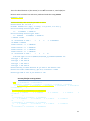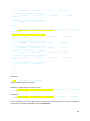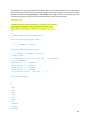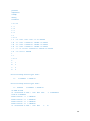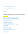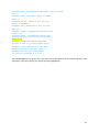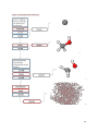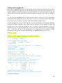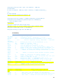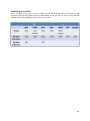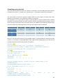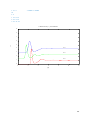
1
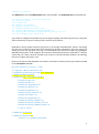
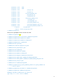
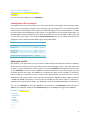
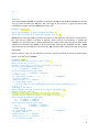
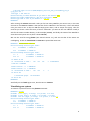
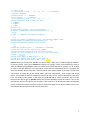
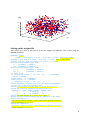
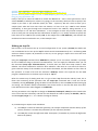
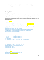
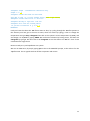
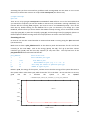
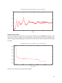
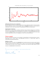
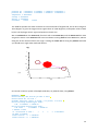
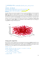
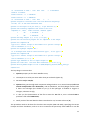
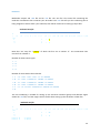
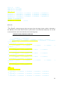
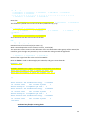
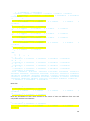
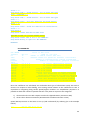
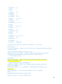
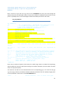
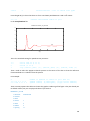
EPSR worked examples By Rowan Hargreaves and Silvia Imberti, updated for EPSR18 on 12 May 2009 In this section we present a number of worked examples, starting with initially quite simple examples working up to more complex ones. Also the description given in the examples becomes briefer in the later examples to avoid repetition. The general procedure followed in these worked examples: 1. Set up the simulation – build an initial configuration, set up the weights files which describe the diffraction data, and set up the input file which controls how EPSR runs; 2. Run the simulation – equilibrate the system’s configuration using MC-only, then introduce the Empirical potential to the refinement, and then accumulate data; and finally 3. Analyse the results. This tutorial has been written from a user point of view, and tries and put together the actions needed to perform a simulation in the order in which they need to be performed. For this reason it may be sometimes oversimplified and does not substitute the need to read the manual in order to understand precisely what it is that you are doing, while running a certain sequence of programs. A reference to the relevant section in the manual is given. Set up (for Windows) There are many ways to run EPSR, but here only one way will be explained so that you can get easily started. Copy the EPSR18 folder under your C drive. The bin folder contains the batch file needed to run EPSR, the mol folder contains some examples of .mol files that you can copy and modify, finally the run folder is where you are supposed to set up your own simulation. In principle you can run your simulation also from other places but not from a folder that contains spaces in the name, so avoid “My Documents” or the Desktop. The run folder, contains a startupfiles subfolder, that contains most of the files that you need in each of your working folders, and to which you will just have to add you data and the other files (essentially .ato, .inp and .wts) that you will create by following the instruction given below. You should have in particular an EPSR.bat file (double-click to run the batch file, right-click and choose edit to edit it) looking like this: set currentdir=%CD% set EPSRroot=C:\EPSR18 set EPSRbin=%EPSRroot%\bin cd %EPSRbin% call epsrsetup cd %currentdir% copy system_commands_windows.txt system_commands.txt title EPSR in %CD% 1 %EPSRbin%\epsrshell The EPSR.bat file calls the EPSRsetup.bat file in the bin folder. The EPSRsetup.bat file looks like this: if defined epsrpath set path=%epsrpath% set epsrpath=%path% title EPSRsetup set EPSRroot=C:\EPSR18 set EPSRbin=%EPSRroot%\bin set EPSRgnu=%EPSRbin%\gnuplot\bin set PGPLOT_DIR=%EPSRbin%\PGPLOT\PGPLOTlib\ set PGPLOT_FONT=%EPSRbin%\PGPLOT\PGPLOT_LIB\grfont.dat set path=%PGPLOT_DIR%;%epsrpath% If you want to modify the way EPSR runs you can play (carefully) with these two files, here a way that works consistently it is given so that you don’t need to worry about it. EPSR doesn’t have a graphic interface (yet) and it is run through a DOS Windows, which is something that was very common in the past but some people may not have seen before. So for the young (sic) among you, here are the basics. The way it is recommended you should run EPSR is by opening an MS-DOS prompt (Start All Programs Accessories Command Prompt or equivalent). It may be useful that you create a shortcut. Another way to open a Command Prompt window is by selecting Run (Start Run) and typing “cmd”. Now you can move to the run folder and create a new folder in which you will copy the files included in the startupfiles subfolder. Microsoft Windows XP [Version 5.1.2600] (C) Copyright 1985-2001 Microsoft Corp. C:\Documents and Settings\si67.CLRC>cd c:\epsr18\run C:\EPSR18\run>mkdir mynewsim C:\EPSR18\run>copy startupfiles mynewsim startupfiles\epsr.bat startupfiles\epsr.sh startupfiles\f0_WaasKirf.dat startupfiles\gnuatoms.txt startupfiles\gnubonds.txt startupfiles\plot_defaults.txt startupfiles\runepsr.txt startupfiles\runepsrbenz.txt startupfiles\system_commands.txt startupfiles\system_commands_linux.txt startupfiles\system_commands_windows.txt 11 file(s) copied. C:\EPSR18\run>cd mynewsim C:\EPSR18\run\mynewsim>dir Directory of C:\EPSR18\run\mynewsim 2 12/05/2009 21:20 <DIR> . 12/05/2009 21:20 <DIR> .. 17/04/2009 16:47 168 epsr.bat 17/04/2009 16:47 140 epsr.sh 17/04/2009 16:47 42,694 f0_WaasKirf.dat 17/04/2009 16:47 849 gnuatoms.txt 17/04/2009 16:47 918 gnubonds.txt 17/04/2009 16:47 17/04/2009 16:47 26 runepsr.txt 17/04/2009 16:47 64 runepsrbenz.txt 17/04/2009 16:47 355 system_commands.txt 17/04/2009 16:47 355 system_commands_linux.txt 17/04/2009 16:47 469 system_commands_windows.txt 58,830 plot_defaults.txt 11 File(s) 2 Dir(s) 104,868 bytes 12,104,372,224 bytes free C:\EPSR18\run\mynewsim> Now you can type epsr in order to launch the shell: C:\EPSR18\run\mynewsim>epsr C:\EPSR18\run\mynewsim>set currentdir=C:\EPSR18\run\mynewsim C:\EPSR18\run\mynewsim>set EPSRroot=C:\EPSR18 C:\EPSR18\run\mynewsim>set EPSRbin=C:\EPSR18\bin C:\EPSR18\run\mynewsim>cd C:\EPSR18\bin C:\EPSR18\bin>call epsrsetup C:\EPSR18\bin>if defined epsrpath set path= C:\EPSR18\bin>set epsrpath=your path C:\EPSR18\bin>title EPSRsetup C:\EPSR18\bin>set EPSRroot=C:\EPSR18 C:\EPSR18\bin>set EPSRbin=C:\EPSR18\bin C:\EPSR18\bin>set EPSRgnu=C:\EPSR18\bin\gnuplot\bin C:\EPSR18\bin>set PGPLOT_DIR=C:\EPSR18\bin\PGPLOT\PGPLOTlib\ C:\EPSR18\bin>set PGPLOT_FONT=C:\EPSR18\bin\PGPLOT\PGPLOT_LIB\grfont.dat C:\EPSR18\bin>set path=your path C:\EPSR18\bin>cd C:\EPSR18\run\mynewsim C:\EPSR18\run\mynewsim>copy system_commands_windows.txt system_commands.txt 1 file(s) copied. C:\EPSR18\run\mynewsim>title EPSR in C:\EPSR18\run\mynewsim C:\EPSR18\run\mynewsim>C:\EPSR18\bin\epsrshell EPSRshell> Welcome to EPSR version 18: 2009-04-01 Type "help" or "?" for a list of commands 3 Binaries folder: %EPSRbin%\ Home folder is: C:\EPSR18\run\mynewsim\ EPSRshell> You can see that the prompt is now EPSRShell>. Amorphous silica example The chemical formula for silica is SiO2. So in our system we have two oxygen atoms for every silicon atom. This is an interesting example as it is possible to get a quite good fit to the experimental data without potential refinement, so we shall try this before bringing in the empirical potential. In order to speed up the initial equilibration of the system it is a good idea to run it at a high temperature, for example 400K, and then equilibrate to the desired temperature, in this case 300K. There is only one set of neutron data used in this example (NeutronSiO2sq.dat) and this has been normalized. The parameters for the reference potential are given in the table below. Silicon Oxygen Epsilon / kJmol-1 0.8 0.65 Sigma / Å 1.03 3.11 Mass / amu 28 16 Charge/ e +2 -1 Atomic number density / atoms Å-3 0.06634 Making an .ato file (See section 4.1 in the manual.) Our first task is to make the file containing the system, the .ato file, in this case this would consist of say 250 silicon atoms and 500 oxygen atoms. The most robust way to make an initial configuration of the system is to use the makemole command (see section 4.3). To use makemole one must create a .mol file to make an .ato files for each atomic type, here one for silicon and one for oxygen. The .mol file is a template file, which can be created in a text editor, but for speed it is often best to take a copy of one already known to work and alter it for the molecule we are trying to make. In this case we have supplied a .mol file for both oxygen and silicon – o.mol and si.mol, respectively. In this case we are treated the two atomic types as “molecules” molecules of one atom and no bonds. The .mol files contain the potential parameters for the atoms. First, we run makemole on our two .mol files. For each file run on makemole creates two files: a .atm file and a .ato file. Below shows makemole being run on o.mol (the oxygen atom .mol file). EPSRshell> makemole o.mol 1 potential temperature vibtemp density ecoredcore 1 7 0 1 1 1 O 0 0 1 7 0 1 4 1 O 0 0 1 O 1 EPSRshell> This creates o.ato and o.atm, and similarly running it on si.mol creates si.ato and si.atm. For now we are only concerned with the .ato files. The next stage of the process is to give the atoms some coordinates using the command fmole (see section 4.4): EPSRshell> fmole o.ato fmole> Type the number of times to perform the shake: 1 fmole> Type the frequency to update the neighbour list (0): 0 fmole asks for how many shakes you want to perform on the molecule, and since our “molecules” in this case are very simple, 1 iteration is sufficient. And it asks for the frequency to update the neighbour list, just type 0 here. Complex molecules may require more. This then prints some output detailing the iterations that fmole is running eventually returning the EPSRshell prompt. fmole should also be run on si.ato. So now these two .ato files have been altered with the atoms given coordinates. Next we need to ‘mix’ our two .ato files to form the system of 250 silicon atoms and 500 oxygen atoms. To do this we run mixato: EPSRshell> mixato mixato> How many .ATO files do you want to mix? 2 mixato> Search for .ato file 1 Filename: o.ato? (Type y to accept, u to go back, e to exit) y minitc> Following molecule types found:1 O 0.10000E+01 0.10000E-01 minitc> Following molecule types found:1 O o 0.10000E+01 0.10000E-01 2.118229 2.44592 no. of molecules to read = 1 1 1 1 0.244592E+01 14.632776 0.06833973 Atomic fraction 1 = 0.10000E+01 no. of molecules to read = 1 1 1 1 1 new atom types in file C:\EPSR\examples_rh\silica_with_silvia\making_ato_an d_inp_2\o.ato Atom type 1 has label O mixato> How many of these molecules do you want in the mixture? 500 mixato> Search for .ato file 2 Filename: o.ato? (Type y to accept, u to go back, e to exit) Filename: si.ato? (Type y to accept, u to go back, e to exit) y minitc> Following molecule types found:1 O 0.10000E+01 0.10000E-01 2 Si 0.10000E+01 0.10000E-01 minitc> Following molecule types found:1 O o 0.10000E+01 0.10000E-01 2 Si si 0.10000E+01 0.10000E-01 2.118229 2.44592 no. of molecules to read = 1 1 1 2 0.244592E+01 14.632776 0.06833973 Atomic fraction 1 = 0.00000E+00 Atomic fraction 2 = 0.10000E+01 no. of molecules to read = 1 1 2 3 5 1 new atom types in file C:\EPSR\examples_rh\silica_with_silvia\making_ato_an d_inp_2\si.ato Atom type 2 has label Si mixato> How many of these molecules do you want in the mixture? 250 mixato> Give atomic number density (per A**3) of mixture: 0.0664 mixato> Type name of file to put mixture in: sio2.ato EPSRshell> After running the mixato command it asks you for how many .ato files you want to mix, in this case we want to mix si.ato and o.ato. It the searches for the .ato files in the directory. It then asks which ones you want to mix: to skip an .ato file simply press return, and to accept one type y. Then for each file you chose it asks how many of these “molecules” you want in the new .ato file. Finally it asks for the atomic number density, in this example (0.0664), and finally the name of the .ato file to write the mixed system out to (here I chose sio2.ato). We can the view file using plotato (see manual section 3.7), and we see that all the atoms are overlapping. So we run introtcluster on sio2.ato to spread the atoms out. EPSRshell> introtcluster sio2.ato minitc> Following molecule types found:1 O 0.10000E+01 0.10000E-01 2 Si 0.10000E+01 0.10000E-01 minitc> Following molecule types found:1 O o 0.10000E+01 0.10000E-01 2 Si si 0.10000E+01 0.10000E-01 19.431013 22.437 no. of molecules to read = 750 750 750 2 750 2 3 0.224370E+02 11295.212 0.06639982 Atomic fraction 1 = 0.66667E+00 Atomic fraction 2 = 0.33333E+00 no. of molecules to read = 750 22.437 22.437 0 rotational groups 750 molecules 22.437 22.437 EPSRshell> And finally we run fmole again once, but this time on sio2.ato. Visualising our system To view our system we can use the plotato command: EPSRshell> plotato Filename: o.ato? (Type y to accept, u to go back, e to exit) Filename: si.ato? (Type y to accept, u to go back, e to exit) Filename: sio2.ato? (Type y to accept, u to go back, e to exit) y minitc> Following molecule types found:1 O 0.10000E+01 0.10000E-01 2 Si 0.10000E+01 0.10000E-01 minitc> Following molecule types found:1 O o 0.10000E+01 0.10000E-01 2 Si si 0.10000E+01 0.10000E-01 6 19.431013 22.437 no. of molecules to read = 750 750 750 2 0.224370E+02 11295.212 0.06639982 Atomic fraction 1 = 0.66667E+00 Atomic fraction 2 = 0.33333E+00 no. of molecules to read = 750 750 2 3 plotato> Decide what kind of output you want:1 = GNUplot 2 = PGplot 3 = JMOL plotato> ? 1 plotato> Specify whether to plot all molecules (1) or several, centred about one particular molecule (2): 1 750 750 plotato> 2 components available for plotting:1 O 2 Si plotato> Give number of components to plot, and component numbers: 2 1 2 plotato> Number of classes read from gnuatoms.txt = 12 plotato> Following atom classes will be plotted:1 O 2 Si plotato> Min and max of plot = -0.120000E+02 0.120000E+02 plotato> For each new bond: type two atom symbols, minimum and maximum lengths of bond, and radius of bond. Type 0 0 0 0 0 to end bond input or ste 0 0 0 0 for stereo pairs. plotato> ? 0 0 0 0 0 plotato> Total number of bonds read in = 6 plotato> Give overall scale factor on atom sizes: 1 plotato> Give plot rotation about x and y (deg): 30 30 plotato allows you to select the .ato file you want to view – here I have cycled through the .ato files by pressing return, until I get to sio2.ato and select it by typing y. There are three different ways to view the .ato file (using GNUplot, PGplot, or JMol), here I select GNUplot by typing 1. Try all of them in order to see the difference. The Jmol option is the last one implemented and it is probably the most user-friendly. Next I select that I want to plot all of the atoms (option 1), and tell it to plot both components by typing 2 1 2 (the first 2 means plot two components – both oxygen and silicon atoms; the 1 refers to the first component and the 2 refers to the second component). We don’t have any bonds in this system so we have to type 0 0 0 0 0 to specify no bonds. The final two responses we have to give to plotato specify how we want GNUplot to plot the system – here I have just kept the atoms at the default size and given a plot rotation of 30 30. Once the plot has appeared we can change the rotation using the mouse. Provided the .ato file has been created correctly we should have something which looks like the plot below. 7 z [Å] 10 5 0 -5 10 -10 5 -10 0 -5 -5 0 x [Å] 5 y [Å] -10 10 Setting up the weights file (See section 5.1.) Next up we have to set up the weights file (.wts file). This is done using the epsrwts command: EPSRshell> epsrwts Filename: o.ato? (Type y to accept, u to go back, e to exit) [here I type return] Filename: si.ato? (Type y to accept, u to go back, e to exit) [here I type return] Filename: sio2.ato? (Type y to accept, u to go back, e to exit) y minitc> Following molecule types found:1 O 0.10000E+01 0.10000E-01 2 Si 0.10000E+01 0.10000E-01 minitc> Following molecule types found:1 O O 0.10000E+01 0.10000E-01 2 Si si 0.10000E+01 0.10000E-01 19.431013 22.437 no. of molecules to read = 750 750 750 2 0.224370E+02 11295.212 0.06639982 Atomic fraction 1 = 0.66667E+00 Atomic fraction 2 = 0.33333E+00 no. of molecules to read = 750 750 2 3 epsrwts> Program to calculate inter- and intra-molecular weightings for DCS, 1st- or 2nd-order difference data. epsrwts> Is the output to be per atom (1), or per molecule (2)? 1 epsrwts> The following components were found in this file Component no., label, atomic fraction, chemical symbol 1 O 0.66667E+00 O 2 Si 0.33333E+00 Si epsrwts> How many samples (1,2, or 3)? (0 to quit) 1 epsrwts> Get the scattering lengths for all components in the sample epsrwts> For component O Type 0 for a natural isotope or mass number for a specific isotope: 0 and its abundance (0.0-1.0): 1 epsrwts> For component Si Type 0 for a natural isotope or mass number for a specific isotope: 0 and its abundance (0.0-1.0): 1 8 epsrwts> Type basename of file to output weights to: sio2 epsrwts> For total data 1 has data been normalised (1) or not (0)? 1 epsrwts> Writing TOTAL weights to file C:\EPSR\examples_rh\silica_with_silvia\ma king_ato_and_inp\sio2tot.wts Firstly it asks you to select the .ato file to create the .wts file for – here I have typed return until it selects sio2.ato, at which point I select it by typing y in the usual way. We then have to specify if the output is per atom or per molecule (select per atom – option 1). We tell it that we have just 1 sample (even when we have more than one dataset it is best to set up a .wts for each dataset individually). It then goes through each component found in the .ato file, asking whether it is a natural isotope or not and their abundances. In this example we have only natural isotopes, and since we have just one isotope we have abundances of 100% (i.e. 1.0). Finally we have to specify the base name for the .wts file (we specify sio2 so the weights file is sio2.EPSR.wts), and whether the total data has been normalized or not, in this example it has. Making an .inp file (See section 5.3) So we have set up an initial configuration for our system (sio2.ato) but before we can run EPSR we have to set up the .inp file which controls how EPSR exactly runs. Performing EPSR with one dataset requires 43 parameters to be set, we are going to require more since we have three datasets. Using the setup epsr command from EPSRshell it prompts you to set various variables. It prompts for lots of different things to do with how EPSR works. You can supply the filename when you call the command (setup epsr <filename base>), if the file does not exist then setup creates it with defaults. The search command is useful for when asked for a file name as it can search for files of a given extension. Many of the variables do not need to be altered, and the defaults are fine. After all the questions it creates a file with the extension .EPSR.inp, which is the input file for the EPSR program. Sometimes this is the best way to setup an .inp file. Often the easiest way of dealing with this is to get a basic .inp file and then edit by hand, this is faster than answering all the questions that the setup epsr command asks. A new one can be created by running setup epsr, giving the base for the filename (in this case sio2) and then exiting (e) and saving. The variables which have defaults have these written in the file and those that don't have defaults have their values flagged as <undefined>. The key parameters in the .inp file to change are fnameato, fnamepcof, ndata (here this needs to be set to 1 since we have 1 dataset), and then for each dataset we need to specify the datafile, .wts file, and the nrtype (nrtype is 3 -- it is a Genie-II histogram format). So, summarising our inputs to the simulation: 1) The .ato file contain the molecular geometry, the sample composition and the density of the system; moreover it contains the parameters for the reference potential 2) The .wts files contain the diffraction data “description” (remember to put also the diffraction data in the folder!) 9 3) The .inp file contains the names of all these indispensable files and the flags we need in order to run the program Running EPSR Equilibration at 10,000K: First off we just want to run a MC simulation without any refinement, so we have to make sure that the potfac parameter in the .inp is set to 0. This means that we are running without the empirical potential being calculated. To speed up the equilibration of the system we want to run at 10000K. To change the temperature that we are running at we have to change the .ato file by using the changeato command: EPSRshell> changeato setup_input_file> File class: "changeato"; file extension: ".ato" Filename: o.ato? (Type y to accept, u to go back, e to exit) [here I type return] Filename: si.ato? (Type y to accept, u to go back, e to exit) [here I type return] Filename: sio2.ato? (Type y to accept, u to go back, e to exit) y setup_input_file> Full filename = C:\EPSR\examples_rh\silica_with_silvia\silica_ 2_mc_equil_10000K\sio2.ato setup_input_file> Reading input file: "sio2.ato" setup_input_file> Run name in input file is different from filename specified C:\EPSR\examples_rh\silica_with_silvia\silica_2_mc_equil_10000K\sio2.ato minitc> Following molecule types found:1 O 0.10000E+01 0.10000E-01 2 Si 0.10000E+01 0.10000E-01 minitc> Following molecule types found:1 O o 0.10000E+01 0.10000E-01 2 Si si 0.10000E+01 0.10000E-01 19.431013 22.437 no. of molecules to read = 750 750 750 2 750 2 3 0.224370E+02 11295.212 0.06639982 Atomic fraction 1 = 0.66667E+00 Atomic fraction 2 = 0.33333E+00 no. of molecules to read = changeato> There are 750 2 types of atom in this file Atom type 1 has label O Atom type 2 has label Si changeato> temp changeato> temp - Temperature of this .ato file. temp: 1000. ? 10000 changeato> temp - Temperature of this .ato file. temp: 10000 ? [here I type return] 10 changeato> stepmi - Intramolecular translation step. stepmi: 0.1 ? e changeato> Current data have not been saved. Type <CR> to save, or q to exit without saving: [here I type return] changeato> Current name of file is "sio2.ato" changeato> Writing to input file "sio2.ato" changeato> File "sio2.ato" already exists. Do you want to overwrite it (y or n)? Y EPSRshell> Firstly we have the select the .ato file we want to alter, by cycling through the .ato files present in the directory until we get to the one we want, which we select by typing y. Then to change the temperature we type temp, changeato then tells us the system’s current temperature (1,000K), and we change it to 10,000K by typing 10000. We confirm this selection by hitting return, and then exit changeato by typing e. We also have to tell changeato to save the data to an .ato file – here I have overwritten the original one. Now are ready to try and equilibrate our system. We can run EPSR once, by simply typing epsr at the in the EPSRshell prompt, it then asks us for the .inp file name. This is a good test that all files are present and correct. 11 Assuming that you have corrected any problems with running EPSR, we now want to run it more than once, to do this we create a run script called runscript.txt (see section 3.4): # simple runscript epsr sio2 Then we run it by typing ss runscript.txt into EPSRshell. EPSR will then run in the .bat window that you started the script but you will be unable to interact with, and EPSR is running indefinitely. To interact with the running EPSR program, you have to start a new EPSRshell prompt – this can be done also by double clicking on the EPSR.bat file in your run directory. This brings up a new EPSRshell, which informs you that it detects that EPSR is already running, we can now either end the script (by typing es), or pause the script (by typing ps), and resuming it later (by typing ss). (There is a full description of EPSR’s running states and script operation in section 3.4 of the manual.) Examining the run So now we can use this second window to examine how EPSR is running using the plot command (see section 3.6). Make sure we have a plot_defaults.txt file in the directory with the basename for the .ato file set correctly (in this case sio2). Look at the energy (p 14), the S(Q) “fits” (p 7) and their Fourier transform g(r) (p 12) and see how they improve (or not) with time. The top few lines of the plot_defaults.txt file should now look like this: plot_defaults Title of this file l 0 Lists available plot types f sio2 b 1 - 3 p 27 Plot using the current or specified plot type npt 27 Number of types of plot File name to plot Block numbers to plot (e.g. 1 2 - 5 9 - 6) Below is p 14, the energy of the system, and we can see that the energy of the system decreases as the system relaxes. Also show is p 7, which shows the “fit” to the data – we can see that it is not very good but this is because the system is still at 10,000K. C:\EPSR\examples_rh\silica_with_silvia\silica_3_mc-only_equil_300K\sio2 2000 U [k J /m o l e ] 1000 Block 1 0 -1000 -2000 -3000 0 50 100 150 200 250 300 350 Iteration number 12 C:\EPSR\examples_rh\silica_with_silvia\silica_3_mc-only_equil_300K\sio2 1.5 1 F (Q ) 0.5 NeutronSiO2sq 0 -0.5 -1 0 5 10 15 20 Q [1/Å] Equilibration at 300K: So next we change the temperature of the system to 300K using the changeato command, in the same way as we did it before, and run EPSR again using the runscript. This time looking at the system’s energy using the plot (p 7) command, we can see that the system relaxes further reducing its energy: C:\EPSR\examples_rh\silica_with_silvia\silica_3_mc-only_equil_300K\sio2 -2600 U [k J /m o l e ] -2800 -3000 -3200 -3400 -3600 0 100 200 300 400 500 Iteration number And we can see that the fit has improved somewhat: 13 C:\EPSR\examples_rh\silica_with_silvia\silica_3_mc-only_equil_300K\sio2 1.5 1 F (Q ) 0.5 NeutronSiO2sq 0 -0.5 -1 0 5 10 15 20 Q [1/Å] Making the fit better prior to refinement We now experiment with the model parameters (the van der Waals parameters and the minimum distance parameters). These can be changed using the changeato command, as we did with the temperature. (In this case the parameters are pretty good, but feel free to experiment.) Beginning the refinement (See section 5.3 in the manual.) To add the refinement of the empirical potential to the simulation we turn it on by changing some of the parameters in the .inp file: 1) we set potfac equal to 1.0; and 2) we set the ereq parameter to be 10 or 20% of the energy – this is roughly 10 to 20% of the energy we have equilibrated too shown in the p 14 plot, in this case we chose 300 kJ/mol. Water example We have 3 diffraction data sets in this example are H2O.mdcs01 (this undeuteriated pure water), D2O.mdcs01 (this is heavy water), and HDO.mdcs01 (and this is a 50:50 molar mixture of deuteriated and undeuteriated water). Making an .ato file We shall construct our system using makemole, like we did with silica but this time we just have one .mol file since we have just one molecule type. Section 4.3 in the manual explains the makemole command and uses water as its first example. The process is very similar for what we did in the silica example. The water.mol file should look like: 4 |0 |1 |2 |3 |4 |5 |6 |7 |8 1 OW 2 * * 3 HW bond OW HW 0.97600 angle HW OW HW 104.50000 |9 |10 |11 |12 |13 |14 |15 |16 | HW 14 potential OW 0.65000E+00 0.31660E+01 potential HW 0.00000E+00 0.00000E+00 temperature 0.300000E+03 vibtemp 0.650000E+02 density 0.100200E+00 ecoredcore 1.00000 3.00000 0.16000E+02 -0.84760E+00 O 0.20000E+01 0.42380E+00 H This .mol file specifies the water molecule to have O-H bonds of length 0.976, and an H-O-H angle of 104.5 degrees. It gives the oxygen atoms sigma values of 3.166 Angstrom, and epsilon values of 0.65 kJ/mol. The hydrogen atoms’ sigma and epsilon are both zero. We run makemole on the water.mol, file which will create water.atm, and the water.ato files. Next we give the atoms in the water.ato file some coordinates running fmole at least 9000 times, without doing this all the atoms will be at the origin. Viewing the water.ato file using the plotato command you should see a single water molecule like this: z [Å] 1 0.5 0 -0.5 -1 -1 -0.5 y [Å] 0 0.5 1 1 0.5 0 x [Å] -0.5 -1 So next we create our system of multiple molecules, say 1000 of them, using mixato: EPSRshell> mixato mixato> How many .ATO files do you want to mix? 1 mixato> Search for .ato file 1 Filename: water.ato? (Type y to accept, u to go back, e to exit) y minitc> Following molecule types found:1 OW 0.10000E+01 0.10000E-01 minitc> Following molecule types found:1 OW water 0.10000E+01 0.10000E-01 2.6891475 3.10516 no. of molecules to read = 1 3 3 2 0.310516E+01 29.94001 0.10020036 Atomic fraction 1 = 0.33333E+00 Atomic fraction 2 = 0.66667E+00 15 no. of molecules to read = 1 3 2 3 2 new atom types in file C:\EPSR\examples_rh\water_2\water_1_making_ato\water .ato Atom type 1 has label OW Atom type 2 has label HW mixato> How many of these molecules do you want in the mixture? 1000 mixato> Give atomic number density (per A**3) of mixture: 0.1002 mixato> Type name of file to put mixture in: water_1000.ato EPSRshell> The main difference from the silica example is that we only have one .ato file to mix. Here I have told mixato to output the 1000 molecules in a file called water_1000.ato. If we looked at water_1000.ato now we would see the same thing as we saw for the water.ato. This is because all the molecules are identical and their atoms are in exactly the same position. To sort this out we spread out the molecules using introtcluster, and then give the intramolecular coordinates some disorder to ensure that the molecules are different from each other using fmole. Run fmole at least for a 5000 times on water_1000.ato. This should leave us with a .ato file ready to run, looking at it using plotato should give something like this: z [Å] 15 10 5 0 -5 -10 -15 -15 -10 -5 x [Å] 0 5 10 15 -15 -10 -5 0 5 10 15 y [Å] Setting up the weights files Next we have to make a weights file for each dataset we have using the epsrwts command. In this example we have three datasets (H2O, D2O, and HDO). So we run epsrwts for each of these. In fact epsrwts does not ask for the dataset names, it only prompts for the .ato file name. Below is a print out of how to set up the .wts file for the nonsubstituted dataset (H2O.mdcs01): EPSRshell> epsrwts Filename: water_1000.ato? (Type y to accept, u to go back, e to exit) y minitc> Following molecule types found:1 OW 0.10000E+01 0.10000E-01 minitc> Following molecule types found:1 OW water_temp 0.10000E+01 0.10000E-01 26.891474 31.0516 16 no. of molecules to read = 1000 3000 3000 2 3000 2 3 0.310516E+02 29940.01 0.10020037 Atomic fraction 1 = 0.33333E+00 Atomic fraction 2 = 0.66667E+00 no. of molecules to read = 1000 epsrwts> Program to calculate inter- and intra-molecular weightings for DCS, 1st- or 2nd-order difference data. epsrwts> Is the output to be per atom (1), or per molecule (2)? 1 epsrwts> The following components were found in this file Component no., label, atomic fraction, chemical symbol 1 OW 0.33333E+00 O 2 HW 0.66667E+00 H epsrwts> How many samples (1,2, or 3)? (0 to quit) 1 epsrwts> Get the scattering lengths for all components in the sample epsrwts> For component OW Type 0 for a natural isotope or mass number for a specific isotope: 0 and its abundance (0.0-1.0): 1 epsrwts> For hydrogen component HW :If it exchanges with atoms on other molecules type 1, if not type 0: 1 epsrwts> For component HW Type 0 for a natural isotope or mass number for a specific isotope: 0 and its abundance (0.0-1.0): 1 epsrwts> Type basename of file to output weights to: H2O epsrwts> For total data 1 has data been normalised (1) or not (0)? 0 epsrwts> Writing TOTAL weights to file C:\EPSR\examples_rh\water\making_water_wt s\H2Otot.wts The key things to note are that: 1. epsrwts prompts you for which .ato file to use; 2. The output is set to be per atom rather than per molecule (option 1); 3. We select only 1 sample; 4. epsrwts then goes through each component asking whether it is a natural isotope (0 if it is a natural isotope and 2 if it is deuterium), and its abundance, and for hydrogen atoms it asks if these can exchange (this should be yes (1) if the hydrogen is bonded to oxygen or nitrogen, otherwise no (0)); 5. It asks you for the basename of the file to write the .wts file to, since I selected H2O it produces a file called H2Otot.wts; 6. Finally it asks if the total data has been normalised or not, here we select not (0). This procedure needs to be done for the other two samples (D2O and HDO), specifying the correct isotopes and their abundance, and so as not to overwrite the previously made .wts file a new file 17 basename has to be given. In the case of the HDO file where there is a mixture of deuterium substituted hydrogen atoms it once you specify a fraction of isotopic substituted atoms epsrwts asks you about the fractions of each. Making an .inp file As with the silica example we use setup epsr, passing the command water_1000 as the basename for the file, to give us the basic .inp file: EPSRshell> setup epsr water_1000 We exit (by typing e) and save the file. A basic .inp file is then created – in this case it is called water_1000.EPSR.inp. Then we edit the file in a text editor, ensuring that define the parameters fnameato, fnamepcof, ndata (here ndata needs to be set to 3 since we have 3 datasets), and then for each dataset we need to specify the datafile, .wts file, and the nrtype (here we have Gudrun histogram type so nrtype = 5 for all files). When we make the basic .inp using setup epsr we only have the parameters for one dataset, so we have to copy and paste the relevant parts twice to be able to define all 3 datasets. The bottom part of the .inp file should look something like this: ... fnameato fnamepcof qmin ndata data 1 water_1000.ato Name of .ato file water_1000.pcof Name of potential coefficients file. 0.05 Minimum value of Q used for potential fits. [0.05] 3 Number of data files to be fit by EPSR datafile wtsfile nrtype rshmin szeros tweak efilereq H2O.mdcs01 H2Otot.wts 5 0.7 0.0 1.0 1.0 Name of data file to be fit Name of weights file for this data set Data type - see User Manual for more details Minimum radius [A] - used for background subtraction Zero limit - 0 means use first data point for Q=0 Scaling factor for this data set. [1.0] Requested energy amplitude for this data set [1.0] D2O.mdcs01 D2Otot.wts 5 0.7 0.0 1.0 1.0 Name of data file to be fit Name of weights file for this data set Data type - see User Manual for more details Minimum radius [A] - used for background subtraction Zero limit - 0 means use first data point for Q=0 Scaling factor for this data set. [1.0] Requested energy amplitude for this data set [1.0] HDO.mdcs01 HDOtot.wts 5 0.7 0.0 1.0 1.0 Name of data file to be fit Name of weights file for this data set Data type - see User Manual for more details Minimum radius [A] - used for background subtraction Zero limit - 0 means use first data point for Q=0 Scaling factor for this data set. [1.0] Requested energy amplitude for this data set [1.0] data 2 datafile wtsfile nrtype rshmin szeros tweak efilereq data 3 datafile wtsfile nrtype rshmin szeros tweak efilereq q 18 Running EPSR MC only to equilibrate First off we just want to run a MC simulation without any refinement, so we have to make sure that potfac is set to 0. As in the silica example we can run EPSR once, by simply typing epsr at the in the EPSRshell prompt, it then asks us for the .inp file name. To run EPSR more than once we can copy the run script we created for the silica to the water run directory, change the file that epsr should run on (in this example water_1000.EPSR.inp), and execute it using the command ss runscript.txt at the EPSRshell. Since this system contains many more atoms it will take a bit longer to run than the silica example. After a while if we look at the energy (p 14 in plot), we see that it has dropped and is levelling off as the system relaxes. The periodic spikes in the energy happen when the intramolecular coordinates are changed all at once to give the system enough intramolecular disorder. C:\EPSR\examples_rh\water_2\water_3_mc_only\water_1000 -15 -20 U [k J /m o l e ] -25 -30 -35 -40 -45 -50 0 50 100 150 200 Iteration number If we look at the fit compared to the data sets (p 7), we see that the fit is not that good since we have not added in the empirical potential yet: 19 C:\EPSR\examples_rh\water_2\water_3_mc_only\water_1000 3.5 3 2.5 HDO F (Q ) 2 1.5 D2O 1 0.5 H2O 0 -0.5 -1 0 5 10 15 20 Q [1/Å] Adding in empirical potential As described in the silica example we turn on refinement by changing some of the variables in the .inp file: must set potfac to 1; we set ereq to 4.0 kJ/mol, which is about 10% of the system energy. To improve the fit it is worth trying to increase ereq, remembering to reset the empirical potential by setting ireset to 1 after each change. 20 Methanol example The system is pure methanol, three samples have been measured (on NIMROD!): a. Deuteriated methanol CD3OD b. Methanol deuteriated on the exchangeable site CH3OD c. Methanol deuteriated on the non-exchangeable sites CD3OH Other information useful to the construction of the simulations are included in the following table: C M O H density [kJ/mol] 0.390 0.065 0.585 0.000 q [e] [Å] 3.700 0.297 1.800 0.000 3.083 -0.728 0.000 0.431 0.089290015 Making an .ato file Take a .mol file and modify it to make a methanol molecule, such as methanol.mol file 4 | |1 |2 | 3 | 4 | 5 | 6 |7 |8 |9 |19 1 C * 3M 2 * 3 O * H bond O H 0.97600 bond C O 1.40000 bond C M 1.08000 angle H O C 104.50000 angle M C M 109.28000 angle M C O 109.28000 potential C 0.39000E+00 0.37000E+01 potential O 0.58500E+00 0.30830E+01 potential M 0.65000E-01 0.18000E+01 potential H 0.00000E+00 0.00000E+00 temperature 0.300000E+03 vibtemp 0.650000E+02 density 0.100200E+00 ecoredcore 1.00000 3.00000 |10 |11 |12 |13 |14 |15 |16 |17 |18 0.12000E+02 0.00000E+00 C 0.16000E+02 -0.72800E+00 O 0.20000E+01 0.00000E+00 H 0.20000E+01 0.43100E+00 H Note that: density 0.100200E+00 This does not need to be the real density of the system at this stage, just something realistic that will allow you to get a decent sized box, e.g. rho=0.1 Å^-3 gives a box of side L=(N/rho)^1/3, where N is the number of atoms in your molecule. Check the box side in the .ato file (see below). Now go to your EPSRshell prompt and type makemole 21 EPSRshell> makemole Filename: methanol.mol? (Type y to accept, u to go back, e to exit) y 1 2 3 bond bond bond angle angle angle rot potential potential potential potential temperature vibtemp density ecoredcore 3 9 3 4 4 1 C 2 M 3 O 4 H 0 3 3 9 3 4 1 C 5 2 1.08 3 1.08 4 1.08 5 1.4 6 1.8965269 2 M 4 1 1.08 3 1.7615492 4 1.7615492 5 2.0309799 3 M 4 1 1.08 2 1.7615492 4 1.7615492 5 2.0309799 4 M 4 1 1.08 2 1.7615492 3 1.7615492 5 2.0309799 5 O 5 1 1.4 6 0.976 2 2.0309799 3 2.0309799 4 2.0309799 6 H 2 5 0.976 1 1.8965269 1 5 1 3 2 3 4 4 C 1 M 3 O 2 H 4 22 EPSRshell> Makemole outputs and .atm file and an .ato file. The .ato file is the actual file containing the molecular coordinates that constitute your 3D model. The .atm file tells you the numbering that is being assigned to atoms within your molecule, that will be used a lot for setting up input files. methanol.atm file 4 | |1 |19 1 2 3 |2 | 3 | 4 | 5 | 6 |7 |8 |9 1 * 5 * 32 * 6 |10 |11 |12 |13 |14 |15 |16 |17 |18 Note that “32” stays for “3 atoms” of which the first one is number “2”. The numeration then restarts from number 5. Number of distinct atom types: 1 C 2 M 3 O 4 H Number of atoms within the molecules 1 C 5 2 1.08 3 1.08 4 1.08 5 1.4 6 1.8965269 2 M 4 1 1.08 3 1.7615492 4 1.7615492 5 2.0309799 3 M 4 1 1.08 2 1.7615492 4 1.7615492 5 2.0309799 4 M 4 1 1.08 2 1.7615492 3 1.7615492 5 2.0309799 5 O 5 1 1.4 6 0.976 2 2.0309799 3 2.0309799 4 2.0309799 6 H This last numbering is needed for setting up the eventual rotational groups and dihedral angles within the .mol file; at a later stage it will be useful when setting up the calculation of SDF files. methanol.mol file 4 | |1 |2 |19 1 2 3 bond O H bond C O | 3 | 4 | 5 | 6 |7 |8 |9 C * O * 3M * H |10 |11 |12 |13 |14 |15 |16 |17 |18 0.97600 1.40000 23 bond C M 1.08000 angle H O C 104.50000 angle M C M 109.28000 angle M C O 109.28000 rot 5 1 potential C 0.39000E+00 0.37000E+01 potential O 0.58500E+00 0.30830E+01 potential M 0.65000E-01 0.18000E+01 potential H 0.00000E+00 0.00000E+00 temperature 0.300000E+03 vibtemp 0.650000E+02 density 0.100200E+00 ecoredcore 1.00000 3.00000 0.12000E+02 0.00000E+00 C 0.16000E+02 -0.72800E+00 O 0.20000E+01 0.00000E+00 H 0.20000E+01 0.43100E+00 H Note that: rot 5 1 I have defined a rotational group, whose axis goes from the Oxygen (atom number 5 indicated in the .atm file) to the Carbon (atom number 1) (see section 4.3 on command makemole). The .ato file is now overwritten and it now shows also the rotational groups. methanol.ato file produced by makemole 1 0.391226E+01 0.300000E+03 0.000E+00 0.100E+00 0.100E+01 0.100E+01 0.100E-01 0.650E+02 6 0.000000E+00 0.000000E+00 0.000000E+00 0.000000E+00 0.000000E+00 0.000000E+00 1 C 1 0.00000E+00 0.00000E+00 0.00000E+00 5 2 0.108E+01 3 0.108E+01 4 0.108E+01 5 0.140E+01 6 0.190E+01 M 2 0.00000E+00 0.00000E+00 0.00000E+00 4 1 0.108E+01 3 0.176E+01 4 0.176E+01 5 0.203E+01 M 3 0.00000E+00 0.00000E+00 0.00000E+00 4 1 0.108E+01 2 0.176E+01 4 0.176E+01 5 0.203E+01 M 4 0.00000E+00 0.00000E+00 0.00000E+00 4 1 0.108E+01 2 0.176E+01 3 0.176E+01 5 0.203E+01 O 5 0.00000E+00 0.00000E+00 0.00000E+00 5 1 0.140E+01 6 0.976E+00 2 0.203E+01 3 0.203E+01 4 0.203E+01 H 6 0.00000E+00 0.00000E+00 0.00000E+00 2 5 0.976E+00 1 0.190E+01 1 ROT 5 1 3 2 3 4 C C 0 0.39000E+00 0.37000E+01 0.12000E+02 0.00000E+00 0.00000E+00 M H 0 0.65000E-01 0.18000E+01 0.20000E+01 0.00000E+00 0.00000E+00 O O 0 0.58500E+00 0.30830E+01 0.16000E+02 -0.72800E+00 0.00000E+00 24 H H 0 0.00000E+00 0.10000E+01 0 0 0 0 0 0 0 1 methanol 0.00000E+00 0.20000E+01 0.43100E+00 0.00000E+00 0.30000E+01 0 0 0 0 0 0 0 0 0 0 0 0 0 0 0 0 0 0 0 0 0 0 0 0 0 0 0 0 0.100000E+01 0.100000E-01 Note that: 6 0.000000E+00 0.000000E+00 0.000000E+00 0.000000E+00 0.000000E+00 The molecule is placed at the centre of the box (coordinates (0, 0, 0)) C 1 0.00000E+00 0.00000E+00 0.00000E+00 5 2 0.108E+01 3 0.108E+01 0.190E+01 M 2 0.00000E+00 0.00000E+00 0.00000E+00 4 0.108E+01 5 0.140E+01 6 All of the atoms are also at the centre of the box. ROT 5 3 1 2 3 4 Rotational axis is from atom 5 (O) to atom 1 (C) With 3 atoms dependent on this rotation: atom 2, 3 and 4 (M). The atom that comes second in the definition of the axis determines what group will be rotated, be careful to get it the right way around: try not to rotate the ceiling around the light bulb! 1 methanol 0.100000E+01 0.100000E-01 Name of the original mol file at the end of the .ato file Now run fmole in order to disentangle your molecule, and give it some disorder. EPSRshell> fmole Filename: methanol.ato? (Type y to accept, u to go back, e to exit) y fmole> Type the number of times to perform the shake: 1000 fmole> Type the frequency to update the neighbour list (0): 1 (…) fmole> Iteration 998 Intramolecular energy: No. of moves tried: 6 No. of moves rejected: fmolec1> Average no. of neighbours per atom = fmole> Iteration 999 Intramolecular energy: No. of moves tried: fmole> Iteration 1000 Intramolecular energy: 5 4 0.10542E+02 6 No. of moves rejected: fmolec1> Average no. of neighbours per atom = No. of moves tried: 0.10152E+02 5 4 0.99766E+01 6 No. of moves rejected: 4 Done fmole methanol.ato file after running fmole 25 1 0.391226E+01 0.300000E+03 0.000E+00 0.929E+00 0.100E+01 0.100E+01 0.100E-01 0.650E+02 6 0.000000E+00 0.000000E+00 0.000000E+00 0.000000E+00 0.000000E+00 0.000000E+00 1 C 1 -0.50274E+00 -0.28944E+00 -0.24052E+00 5 2 0.108E+01 3 0.108E+01 4 0.108E+01 5 0.140E+01 6 0.190E+01 M 2 -0.11533E+01 -0.97934E+00 0.45225E+00 4 1 0.108E+01 3 0.176E+01 4 0.176E+01 5 0.203E+01 M 3 -0.12542E+01 0.38858E+00 -0.67153E+00 4 1 0.108E+01 2 0.176E+01 4 0.176E+01 5 0.203E+01 M 4 -0.15029E+00 -0.10603E+01 -0.86880E+00 4 1 0.108E+01 2 0.176E+01 3 0.176E+01 5 0.203E+01 O 5 0.62257E+00 0.27662E+00 0.30857E+00 5 1 0.140E+01 6 0.976E+00 2 0.203E+01 3 0.203E+01 4 0.203E+01 H 6 0.59375E+00 0.11747E+01 0.62659E-01 2 5 0.976E+00 1 0.190E+01 1 ROT 5 1 3 2 3 4 C C 0 0.39000E+00 0.37000E+01 0.12000E+02 0.00000E+00 0.00000E+00 M H 0 0.65000E-01 0.18000E+01 0.20000E+01 0.00000E+00 0.00000E+00 O O 0 0.58500E+00 0.30830E+01 0.16000E+02 -0.72800E+00 0.00000E+00 H H 0 0.00000E+00 0.00000E+00 0.20000E+01 0.43100E+00 0.00000E+00 0.10000E+01 0.30000E+01 23976 1149980312 313375245 763635818 1726722452 2125952865 2104917671 809766993 699594297 1667287044 959103680 1057147157 643295378 1118800511 1410340799 1064918654 311045925 989545951 773664677 2116227401 1149980312 1979976970 447123753 1876842048 801051620 353008694 477082433 1432739048 1340056068 1684201980 44129405 1587877127 2137358203 409080103 1199857746 1 methanol 0.100000E+01 0.100000E-01 Note that: C 1 -0.50274E+00 -0.28944E+00 -0.24052E+00 5 2 0.108E+01 3 0.108E+01 0.190E+01 M 2 -0.11533E+01 -0.97934E+00 0.45225E+00 4 0.108E+01 5 0.140E+01 6 Now the coordinates of each atom relative to the center of mass are different from zero and compatible with the bond distance C 1 -0.50274E+00 -0.28944E+00 -0.24052E+00 5 2 0.108E+01 3 0.108E+01 0.190E+01 4 0.108E+01 5 0.140E+01 6 26 This is the bond distance: C (aka atom1) is at 1.08Å from atom 2, 3 and 4 (M) etc. Now we want to make a box with many methanol molecules using mixato EPSRshell> mixato mixato> How many .ATO files do you want to mix? 1 mixato> Search for .ato file 1 Filename: methanol.ato? (Type y to accept, u to go back, e to exit) y minitc> Following molecule types found:1 C 0.10000E+01 0.10000E-01 minitc> Following molecule types found:1 C methanol 0.10000E+01 0.10000E-01 3.3881166 3.91226 no. of molecules to read = 1 6 6 4 6 4 10 0.391226E+01 59.880188 0.10020009 Atomic fraction 1 = 0.16667E+00 Atomic fraction 2 = 0.50000E+00 Atomic fraction 3 = 0.16667E+00 Atomic fraction 4 = 0.16667E+00 no. of molecules to read = 1 4 new atom types in file C:\EPSR17\run\met\met_4_ato2mixato\methanol.ato Atom type 1 has label C Atom type 2 has label M Atom type 3 has label O Atom type 4 has label H mixato> How many of these molecules do you want in the mixture? 1000 mixato> Give atomic number density (per A**3) of mixture: 0.08929 mixato> Type name of file to put mixture in: met met.ato file after running mixato 1000 0.406552E+02 0.300000E+03 0.000E+00 0.929E+00 0.100E+01 0.100E+01 0.100E-01 0.650E+02 6 0.000000E+00 0.000000E+00 0.000000E+00 0.000000E+00 0.000000E+00 0.000000E+00 1 C 1 -0.50274E+00 -0.28944E+00 -0.24052E+00 5 2 0.108E+01 3 0.108E+01 4 0.108E+01 5 0.140E+01 6 0.190E+01 M 2 -0.11533E+01 -0.97934E+00 0.45225E+00 4 1 0.108E+01 3 0.176E+01 4 0.176E+01 5 0.203E+01 M 3 -0.12542E+01 0.38858E+00 -0.67153E+00 4 1 0.108E+01 2 0.176E+01 4 0.176E+01 5 0.203E+01 M 4 -0.15029E+00 -0.10603E+01 -0.86880E+00 27 4 1 0.108E+01 2 0.176E+01 3 0.176E+01 5 0.203E+01 5 0.62257E+00 0.27662E+00 0.30857E+00 5 1 0.140E+01 6 0.976E+00 2 0.203E+01 3 0.203E+01 4 0.203E+01 H 6 0.59375E+00 0.11747E+01 0.62659E-01 2 5 0.976E+00 1 0.190E+01 1 ROT 5 1 3 2 3 4 6 0.000000E+00 0.000000E+00 0.000000E+00 0.000000E+00 0.000000E+00 0.000000E+00 2 C 1 -0.50274E+00 -0.28944E+00 -0.24052E+00 5 2 0.108E+01 3 0.108E+01 4 0.108E+01 5 0.140E+01 6 0.190E+01 M 2 -0.11533E+01 -0.97934E+00 0.45225E+00 4 1 0.108E+01 3 0.176E+01 4 0.176E+01 5 0.203E+01 M 3 -0.12542E+01 0.38858E+00 -0.67153E+00 4 1 0.108E+01 2 0.176E+01 4 0.176E+01 5 0.203E+01 M 4 -0.15029E+00 -0.10603E+01 -0.86880E+00 4 1 0.108E+01 2 0.176E+01 3 0.176E+01 5 0.203E+01 O 5 0.62257E+00 0.27662E+00 0.30857E+00 5 1 0.140E+01 6 0.976E+00 2 0.203E+01 3 0.203E+01 4 0.203E+01 H 6 0.59375E+00 0.11747E+01 0.62659E-01 2 5 0.976E+00 1 0.190E+01 1 ROT 5 1 3 2 3 4 O Etc.etc. Note that: 1000 0.406552E+02 0.300000E+03 We have 1000 molecules in the box Molecule 1 (EPSR kindly counts them for us) 6 0.000000E+00 0.000000E+00 1 0.000000E+00 0.000000E+00 0.000000E+00 0.000000E+00 0.000000E+00 0.000000E+00 0.000000E+00 0.000000E+00 Molecule 2 6 0.000000E+00 0.000000E+00 2 All the molecules are at the origin and they all have the same orientation in space. To randomize their positions and their orientations we run introtcluster. 28 The molecules are now nicely scattered throughout the box, but their intramolecular coordinates are all the same (they all have the exact same bond length and internal angles), so we give them some thermal disorder by running fmole again. While fmole on the single molecule is very quick, this time it will take a lot longer as it has to do the same operation on many many molecules. EPSRshell> fmole Filename: met.ato? (Type y to accept, u to go back, e to exit) y fmole> Type the number of times to perform the shake: 9999 fmole> Type the frequency to update the neighbour list (0): 0 met met C:\EPSR17\run\met\met_6_introt2fmole\met.ato minitc> Following molecule types found:- 1 C 0.10000E+01 0.10000E-01 minitc> Following molecule types found:- 1 C methanol 0.10000E+01 0.10000E-01 35.20844 40.6552 no. of molecules to read = 1000 6000 6000 4 6000 4 10 0.406552E+02 67196.76 0.089290015 Atomic fraction 1 = 0.16667E+00 Atomic fraction 2 = 0.50000E+00 Atomic fraction 3 = 0.16667E+00 Atomic fraction 4 = 0.16667E+00 no. of molecules to read = 1000 fmole> makemole methanol 1 2 3 bond bond bond angle angle angle rot potential potential potential 29 potential temperature vibtemp density ecoredcore 3 9 3 4 4 1 C 2 M 3 O 4 H 0 3 3 9 3 4 1 C 5 2 1.08 3 1.08 4 1.08 5 1.4 6 1.8965269 2 M 4 1 1.08 3 1.7615492 4 1.7615492 5 2.0309799 3 M 4 1 1.08 2 1.7615492 4 1.7615492 5 2.0309799 4 M 4 1 1.08 2 1.7615492 3 1.7615492 5 2.0309799 5 O 5 1 1.4 6 0.976 2 2.0309799 3 2.0309799 4 2.0309799 6 H 2 5 0.976 1 1.8965269 1 5 1 3 2 3 4 4 C 1 M 3 O 2 H 4 minitc> Following molecule types found:- 1 C 0.10000E+01 0.10000E-01 minitc> Following molecule types found:- 1 C methanol 0.10000E+01 0.10000E-01 35.20844 40.6552 no. of molecules to read = 1000 6000 6000 4 6000 4 10 0.406552E+02 67196.76 0.089290015 Atomic fraction 1 = 0.16667E+00 Atomic fraction 2 = 0.50000E+00 Atomic fraction 3 = 0.16667E+00 Atomic fraction 4 = 0.16667E+00 no. of molecules to read = 1000 30 update_ato> methanol.ato (…) fmole> Iteration 97 Intramolecular energy: No. of moves tried: fmole> Iteration 6000 No. of moves rejected: 98 Intramolecular energy: No. of moves tried: fmole> Iteration 0.18956E+02 4497 0.19084E+02 6000 No. of moves rejected: 99 Intramolecular energy: No. of moves tried: 4522 0.19046E+02 6000 No. of moves rejected: 4481 Done fmole Note on rotational groups: Now, when mixing molecules with rotational groups (e.g. methanol) and molecules without (e.g. water), EPSR may “switch off” the option to rotate the groups. It is always better to double-check this (and if necessary switch it back on) using the changeato command. EPSRshell> changeato setup_input_file> File class: "changeato"; file extension: ".ato" Filename: met.ato? (Type y to accept, u to go back, e to exit) y setup_input_file> Full filename = C:\EPSR17\run\met\met_6_fmole\met.ato setup_input_file> Reading input file: "met.ato" setup_input_file> Run name in input file is different from filename specified C:\EPSR17\run\met\met_6_fmole\met.ato minitc> Following molecule types found:1 C 0.10000E+01 0.10000E-01 minitc> Following molecule types found:1 C methanol 0.10000E+01 0.10000E-01 35.20844 40.6552 no. of molecules to read = 1000 6000 6000 4 6000 4 10 0.406552E+02 67196.76 0.089290015 Atomic fraction 1 = 0.16667E+00 Atomic fraction 2 = 0.50000E+00 Atomic fraction 3 = 0.16667E+00 Atomic fraction 4 = 0.16667E+00 no. of molecules to read = changeato> There are 1000 4 types of atom in this file Atom type 1 has label C Atom type 2 has label M Atom type 3 has label O Atom type 4 has label H changeato> 31 changeato> bond - Intra-molecular bond lengths. Type y to change. bond: n ? changeato> label - Atom labels. Type y to change. label: n ? changeato> density - Density of this .ato file. density: 0.089290015 ? changeato> temp - Temperature of this .ato file. temp: 300. ? changeato> stepmi - Intramolecular translation step. stepmi: 1.02 ? changeato> stepri - Intramolecular rotation step. stepri: 1. ?e changeato> Current data have not been saved. Type <CR> to save, or q to exit without saving: changeato> Current name of file is "met.ato" changeato> Writing to input file "met.ato" changeato> File "met.ato" already exists. Do you want to overwrite it (y or n)? y The variable stepri has to be put at 1 if you want to turn on rotations of the rotational groups in the simulation. (Lines that require your input have been highlighted.) 32 33 Setting up the weights file We have to run epsrwts once for each of the samples we have measured, including once for each of the isotopic compositions. We have only one simulation box for a given chemical composition of our sample, regardless of how many different isotopic substitution we have performed on it. But we need to inform the program about these isotopically substituted samples. This is what the “weights” do. For each atom type epsrwts will ask us what the mass number is (we use “0” for natural isotopic composition), and the abundance of this atom type (“1” if all of it is the same isotopic composition, or a fraction number if you have a mixture). (See also the water example on this.) For each hydrogen atom we have in our .ato file, we will be asked whether the hydrogen exchanges with atoms on other molecules. This happens only for hydrogen atoms bonded to oxygen and nitrogen atoms. This is important, because in your real sample, a mixture ofCD3OD in H2O at 1:1 molar fraction say, you will have effectively a 1:2 ratio D:H in your sample on all of the exchangeable sites -- in fact you will end up with CD3O(H/D=2:1) in (H/D=2:1)2O. So the weight for those exchangeable sites needs to be calculated accordingly, and epsrwts kindly does this for you. EPSRshell> epsrwts Filename: met.ato? (Type y to accept, u to go back, e to exit) y minitc> Following molecule types found:1 C 0.10000E+01 0.10000E-01 minitc> Following molecule types found:1 C methanol 0.10000E+01 0.10000E-01 35.20844 40.6552 no. of molecules to read = 1000 6000 6000 4 6000 4 10 0.406552E+02 67196.76 0.089290015 Atomic fraction 1 = 0.16667E+00 Atomic fraction 2 = 0.50000E+00 Atomic fraction 3 = 0.16667E+00 Atomic fraction 4 = 0.16667E+00 no. of molecules to read = 1000 epsrwts> Program to calculate inter- and intra-molecular weightings for DCS, 1st- or 2nd-order difference data. epsrwts> Is the output to be per atom (1), or per molecule (2)? 1 epsrwts> The following components were found in this file Component no., label, atomic fraction, chemical symbol 1 C 0.16667E+00 C 2 M 0.50000E+00 H 3 O 0.16667E+00 O 4 H 0.16667E+00 H epsrwts> How many samples (1,2, or 3)? (0 to quit) 1 epsrwts> Get the scattering lengths for all components in the sample epsrwts> For component C 34 Type 0 for a natural isotope or mass number for a specific isotope: 0 and its abundance (0.0-1.0): 1 epsrwts> For hydrogen component M :- If it exchanges with atoms on other molecules type 1, if not type 0: 0 epsrwts> For component M Type 0 for a natural isotope or mass number for a specific isotope: 2 and its abundance (0.0-1.0): 1 epsrwts> For component O Type 0 for a natural isotope or mass number for a specific isotope: 0 and its abundance (0.0-1.0): 1 epsrwts> For hydrogen component H :- If it exchanges with atoms on other molecules type 1, if not type 0: 1 epsrwts> For component H Type 0 for a natural isotope or mass number for a specific isotope: 2 and its abundance (0.0-1.0): 1 epsrwts> Type basename of file to output weights to: cd3od_ epsrwts> For total data 1 has data been normalised (1) or not (0)? 0 epsrwts> Writing TOTAL weights to file C:\EPSR17\run\met\met_7_wts\cd3od_tot.wts Summarising in a table the sequence of answers for this example: exch C M O H 0 1 CD3OD mass 0 2 0 2 % 1 1 1 1 exch 0 1 CD3OH mass 0 2 0 0 % 1 1 1 1 exch 0 1 CH3OD mass 0 0 0 2 % 1 1 1 1 Note that: epsrwts> Type basename of file to output weights to: cd3od_ The output file will be called cd3od_tot.wts epsrwts> For total data 1 has data been normalised (1) or not (0)? 0 Files output by Gudrun (.mdcs01) are not normalised (e.g. divided by the total cross section of the sample). Making an .inp file Now we first make setup epsr write the input file and then we modify it. The setup menu, as with the plot menu, goes round in a loop asking you the same questions forever until you exit it (after you have modified all of the variables you want to modify). In some case you may be better off by just creating the .inp file and then editing it directly from a normal text editor, as in the following example (this produces a file called met.EPSR.inp) EPSRshell> setup epsr 35 setup_input_file> File class: "epsr"; file extension: ".EPSR.inp" File Not Found No files of extension ".EPSR.inp" found in directory "C:\EPSR17\run\met\met_7_ ts\" No files selected... Type the required filename with extension: met setup_input_file> Full filename = C:\EPSR17\run\met\met_7_wts\met.EPSR.inp setup_input_file> Problems with specified input file: met.EPSR.inp - will use default values Setup epsr> e Setup epsr> Current data have not been saved. Type <CR> to save, or q to exit without saving: (Here I pressed “enter”) Setup epsr> Current name of file is "met.EPSR.inp" Setup epsr> Writing to input file "met.EPSR.inp" met.EPSR.inp met.EPSR feedback potfac ereq efilereq sizefactor nq qstep ireset iinit ntimes niter nsumt reset] intra [100] inter rho cellst fwhm fwhmq nsmoop fnameato fnamepcof qmin ndata data 0.8 0.0 5.0 1.0 400 0.05 1 1 5 1 -1 Title of this file Confidence factor - should be < 1. [0.8] 1.0 to enable potential refinement, 0.0 to inhibit Overall requested energy amplitude - overrules Multiplying factor for box dimension. [1.0] Number of Q values. [400] Size of Q step [1/A]. [0.05] Sets the Empirical Potential to zero Sets accumulators to zero. Recalculates r and Q. [1] Number of MC cycles between potential refinements. [5] Number of potential refinements before exitting. [1] Number of iterations already accumulated. [-1 with 100 Number of molecule moves between molecule shakes. 5 Number of iterations in running averages. [5] 0.1 Atomic number density - will be derived from .ato file 0.03 Size of r step [A]. [0.03] 0.0 Resolution width - Q independent term. [0.0] 0.02 Resolution width - Q dependent term. [0.02 for SLS] 1 1 means background subtraction is ON, 0 means OFF <undefined> Name of .ato file <undefined> Name of potential coefficients file. 0.05 Minimum value of Q used for potential fits. [0.05] 1 Number of data files to be fit by EPSR 1 datafile wtsfile set nrtype rshmin szeros <undefined> <undefined> 5 0.7 0.0 Name of data file to be fit Name of weights file for this data Data type - see User Manual for more details Minimum radius [A] - used for background subtraction Zero limit - 0 means use first data point for Q=0 36 tweak efilereq q 1.0 1.0 Scaling factor for this data set. [1.0] Requested energy amplitude for this data set [1.0] At this point we actually match each dataset with its own .wts file; it’s normally good to have them in some sort of logical order, such as H/D ratio. (…) fnameato met.ato Name of .ato file fnamepcof met.pcof Name of potential coefficients file. qmin 0.05 Minimum value of Q used for potential fits. [0.05] ndata 3 Number of data files to be fit by EPSR data 1 datafile wtsfile set nrtype rshmin szeros tweak efilereq data 5 0.7 0.0 1.0 1.0 Name of data file to be fit Name of weights file for this data Data type - see User Manual for more details Minimum radius [A] - used for background subtraction Zero limit - 0 means use first data point for Q=0 Scaling factor for this data set. [1.0] Requested energy amplitude for this data set [1.0] 2 datafile wtsfile set nrtype rshmin szeros tweak efilereq data NIMROD00000045.mdcs01 cd3od_tot.wts NIMROD00000057.mdcs01 cd3oh_tot.wts 5 0.7 0.0 1.0 1.0 Name of data file to be fit Name of weights file for this data Data type - see User Manual for more details Minimum radius [A] - used for background subtraction Zero limit - 0 means use first data point for Q=0 Scaling factor for this data set. [1.0] Requested energy amplitude for this data set [1.0] 3 datafile wtsfile nrtype rshmin szeros tweak efilereq q NIMROD00000050.mdcs01 Name of data file to be fit ch3od.wts Name of weights file for this data set 5 Data type - see User Manual for more details 0.7 Minimum radius [A] - used for background subtraction 0.0 Zero limit - 0 means use first data point for Q=0 1.0 Scaling factor for this data set. [1.0] 1.0 Requested energy amplitude for this data set [1.0] Note: nrtype 5 Data type - see User Manual for more details This is the correct filetype for files output by Gudrun. Running EPSR Now we check first of all if the program will run, by typing epsr met where “met” is the name of your .inp file. The first time you do this, it doesn’t find the met.pcof file, but it doesn’t matter because it will create it. Afterwards you can create a script to run EPSR multiple times. Now continue to equilibrating, refining and accumulating as explained in the previous examples. 37 Examining the results When visualising your results, it may be useful to know the meaning of all the extension of the numerous files output by EPSR, listed in the table below. In this way you can also use you preferred program other than the plot routine to look at your results. 38 Visualising your partials The partial pair correlation functions (or “partials”) are written in the met.EPSR.g01 file asa sequence of columns of the form: r, partial1, error, partial2, error…. The header contains this information: # r C-C C-M C-O C-H M-M M-O M-H O-O O-H H-H The total number of functions is given by N(N+1) where N is the number of distinct atom types defined in the simulation. In this example, we have N=4 (C,M,O,H). For convenience it is a good idea to make a look-up table to help you identify which columns correspond to which partial pair correlation function. Follow the example below and make sure you enter the atoms in the same order as you have them in your .mol file. The numbering sequence goes from left to right only numbering distinct pairs (e.g. upper right corner plus diagonal). C 1 C M O H M 2 5 O 3 6 8 H 4 7 9 10 Now you can plot these functions from the plot routine by typing pt 8 and choosing the block numbers. For example by typing b 8 9 10 (or b 8 – 10) and then typing again p, this will plot the individual O-O, O-H and H-H intermolecular correlations. EPSRshell> plot setup_input_file> File class: "plot"; file extension: "plot_defaults.txt" setup_input_file> Full filename = C:\EPSR17\run\met_11_accumulated\plot_default.txt setup_input_file> Reading input file: "plot_defaults.txt" plot> pt 8 pt 8 - Sets the specified plot type plot> type - Type of plot type: 8 - EPSR site-site g(r) ? b 8 - 10 find_ncolumn> 10 10 find_ncolumn> 8 21 2 setup_plot_filenames> There are 2 2 10 10 blocks in the file C:\EPSR17\run\met_11_accu mulated\met.EPSR.g01 setup_blocknumbers> Number of plotting columns: 3 plot> b - Block numbers to plot (e.g. 1 2 - 5 9 - 6) b: 8 - 10 ? p find_ncolumn> 10 10 find_ncolumn> 8 21 2 2 2 setup_plot_filenames> There are C:\EPSR17\run\met_11_accumulated\met.EPSR.g01 setup_blocknumbers> Number of plotting columns: 10 10 blocks in the file 3 39 1.0 1.0 1.000000 1.000000 nn 2 2 1 2 2 8 10 2 2 2 9 16 3 2 2 10 18 C:\EPSR17\run\met_11_accumulated\met 9 8 7 6 g(r) 5 H-H 4 3 O-H 2 O-O 1 0 0 2 4 6 8 10 12 r [Å] 40 Spherical harmonics Among many analysis routines, one of the most elaborate is the one that calculates the representation in terms of certain special functions called spherical harmonics of the correlations between the atoms correlations (see chapter 7). This sort of information is reconstructed from the simulation box (and averaged over many configurations of the molecules in the box), and it’s a useful 3-dimensional view of the information at least in part already contained within the partial pair correlation functions. The best way to learn how to use them is to see some examples (some are in the manual and we have added one here for the methanol example) and start thinking about your own molecule. The calculation is performed in two steps: 1) Calculation of the spherical harmonics coefficients configurations) 2) Representation of the Function obtained (accumulating over several The initial calculation doesn’t require much thinking about what you want to do: just how accurate you may want you calculation to be (e.g. where to truncate your expansion). A typical starting value is given in the example below as l1values l2values lvalues 0 1 2 3 4 0 1 2 3 4 0 1 2 3 4 L1 values (separated by spaces) L2 values (separated by spaces) L values (separated by spaces) We consider two molecules, one at the centre with a specific orientation and we go and look at the position of orientation of another molecule (of the same type or of a different type) with respect to this first one. You need to have some basic knowledge about the geometry of your molecule, because the presence of symmetries simplifies the calculation. Here it is required to provide the category of a rotational symmetry axis of the molecule, according to molecular point group symmetry. A symmetry axis is an axis around which a rotation by 360/n results in a molecule indistinguishable from the original. This is also called an n-fold rotational axis and abbreviated Cn. Examples are the C2 in water and the C3 in ammonia. A molecule can have more than one symmetry axis; the one with the highest n is called the principal axis, and by convention is assigned the z-axis in a Cartesian coordinate system. If the molecule has cylindrical symmetry (e.g. an OH ion), n is 0 and 1 if the molecule doesn’t have any rotational symmetry axis then it belongs to C1. n1step n2step 1 1 Step in N1 values Step in N2 values Then we have to define a frame reference attached to each of the two molecules, bearing in mind atom-c axisc1 axisc2 atom-s axiss1 axiss2 O z x O z x 6 1 6 1 Central molecule - list of centre atom types First axis definition for central molecule Second axis definition for central molecule Second molecule - list of centre atom types First axis definition for second molecule Second axis definition for second molecule 41 Quoting from the manual: “For the first axis (z in this example) the specified axis is assumed to run from the centre of the molecule to the mid-point of the specified atoms. (Several atoms can be specified.) For the second axis it may not be possible to assign a set of atoms which lie along the specified axis, so instead a vector is drawn from the centre of the molecule to the point defined by the set of specified atoms, and the second axis is assumed to lie in the plane defined by the this vector and the first axis: its precise direction is determined from the requirement that it must be orthogonal to the first axis. The molecule as defined MUST have at least one plane of mirror symmetry and at least one of the mirror symmetry planes must be coincident with the z-x plane. If such a plane does not exist in the real molecule, then mirror symmetry about the z-x plane will be imposed on the estimated distribution functions, and it likely they could be misleading.” Here follows an example of how to setup an input file that calculates the spherical harmonics coefficients. EPSRshell> setup sharm setup_input_file> File class: "sharm"; file extension: ".SHARM.dat" File Not Found No files of extension ".SHARM.dat" found in directory "C:\EPSR17\run\met\met__sharm\" No files selected... Type the required filename with extension: met setup_input_file> Full filename = C:\EPSR17\run\met\met_12_sharm\met.SHARM.dat setup_input_file> Problems with specified input file: met.SHARM.dat - will use default values Setup sharm> Setup sharm> fnameato - Name of .ato file fnameato: <undefined> ? met Attempting to read file: met.ato minitc> Following molecule types found:1 C 0.10000E+01 0.10000E-01 minitc> Following molecule types found:1 C methanol 0.26816E+00 0.79901E-02 35.20844 40.6552 no. of molecules to read = 1000 6000 6000 4 6000 4 10 0.406552E+02 67196.76 0.089290015 Atomic fraction 1 = 0.16667E+00 Atomic fraction 2 = 0.50000E+00 Atomic fraction 3 = 0.16667E+00 Atomic fraction 4 = 0.16667E+00 no. of molecules to read = There are 1000 4 types of atom in this file Atom type 1 has label C Atom type 2 has label M 42 Atom type 3 has label O Atom type 4 has label H Setup sharm> fnameato - Name of .ato file fnameato: met.ato ? Setup sharm> nr - Number of radius values (max 200) nr: 100 ? Setup sharm> rmax - Maximum radius for spherical harmonic coefficients rmax: 10 ? Setup sharm> nsumt - Number of configurations already accumulated nsumt: 0 ? Setup sharm> ncoeffs - Number of coefficients (program calculates this) ncoeffs: 0 ? Setup sharm> l1values - L1 values (separated by spaces) l1values: 0 ? 0 1 2 3 4 Setup sharm> l1values - L1 values (separated by spaces) l1values: 0 1 2 3 4 ? Setup sharm> l2values - L2 values (separated by spaces) l2values: 0 ? 0 1 2 3 4 Setup sharm> l2values - L2 values (separated by spaces) l2values: 0 1 2 3 4 ? Setup sharm> lvalues - L values (separated by spaces) lvalues: 0 ? 0 1 2 3 4 Setup sharm> lvalues - L values (separated by spaces) l2values: 0 1 2 3 4 ? Setup sharm> n1step - Step in N1 values n1step: 0 ? 1 Setup sharm> n1step - Step in N1 values n1step: 1 ? Setup sharm> n2step - Step in N2 values n2step: 0 ? 1 Setup sharm> n2step - Step in N2 values n2step: 1 ? Setup sharm> atom-c - Central molecule - list of centre atom types atom-c: <undefined> ? O Setup sharm> atom-c - Central molecule - list of centre atom types atom-c: O ? Setup sharm> axisc1 - First axis definition for central molecule axisc1: <undefined> ? z 6 Setup sharm> axisc1 - First axis definition for central molecule axisc1: z 6 ? Setup sharm> axisc2 - Second axis definition for central molecule axisc2: <undefined> ? x 1 Setup sharm> axisc2 - Second axis definition for central molecule 43 axisc2: x 1 ? Setup sharm> atom-s - Second molecule - list of centre atom types atom-s: <undefined> ? O Setup sharm> atom-s - Second molecule - list of centre atom types atom-s: O ? Setup sharm> axiss1 - First axis definition for second molecule axiss1: z 6 ? Setup sharm> axiss2 - Second axis definition for second molecule axiss2: x 1 ? Setup sharm> e Setup sharm> Current data have not been saved. Type <CR> to save, or q to exit without saving: Setup sharm> Current name of file is "met.SHARM.dat" Setup sharm> Writing to input file "met.SHARM.dat" EPSRshell> met.SHARM.dat met.SHARM fnameato nr rmax nsumt ncoeffs this) l1values l2values lvalues n1step n2step atom-c axisc1 axisc2 atom-s axiss1 axiss2 q met.ato 10 10 0 0 0 0 0 1 1 O z x O z x 1 2 3 4 1 2 3 4 1 2 3 4 6 1 6 1 Title of this file Name of .ato file Number of radius values (max 200) Maximum radius for spherical harmonic coefficients Number of configurations already accumulated Number of coefficients (program calculates L1 values (separated by spaces) L2 values (separated by spaces) L values (separated by spaces) Step in N1 values Step in N2 values Central molecule - list of centre atom types First axis definition for central molecule Second axis definition for central molecule Second molecule - list of centre atom types First axis definition for second molecule Second axis definition for second molecule Once the coefficients are calculated, we can decide what type of information exactly we want to extract. This requires a little thinking, since setting certain indexes to the coefficients to zero is equivalent to integrating along certain spatial/angular variables. For simplification purposes it is possible to divide the number of possible function I may want to inspect in two categories: 1) 2) where molecule 2 sits with respect to molecule 1 (Spatial Density Function or SDF) what is their relative orientations (Orientational correlation Function or OCF) Spatial Density Function is the easier to set up (and understand!) by selecting (as in the example below): 1 0 use l1 and l2 (1 or 0) 44 1 0 0 1 use n1 and n2 (1 or 0) use m2 (1 or 0) vary (thetal, phil) (1), (thetam, phim) (2), (thetam, chim) (3) The Orientational Correlation Function properly said is selected by setting 1 1 1 1 1 use l1 and l2 (1 or 0) use n1 and n2 (1 or 0) use m2 (1 or 0) and then choosing option 2 or 3 in the following line: 2 vary (thetal, phil) (1), (thetam, phim) (2), (thetam, chim) (3) The meaning of what we are plotting now depends on how we have actually setup our initial axes on the molecules and an understanding of the Euler angles representation. Quoting from the manual again: “A description of Euler angles can be found in a number of textbooks. The definitions used here are based on Theory of Molecular Fluids Volume 1 – Fundamentals, C G Gray and K E Gubbins, Oxford University Press, 1984, which also gives an excellent account of the spherical harmonic functions. The order of the rotations being used here to get to the final orientation is important. The entity is first rotated by an amount φ about the initial z-axis, then by an amount θ about the new y-axis, finally by an amount χ about the revised z-axis that is generated by the second rotation. All rotations are in the direction of a clockwise screw along the positive axis. They can also be performed in reverse order but rotating about the (fixed) laboratory axes throughout. “ TODO It also requires a bit of graphic construction, in order to build the image of our first reference molecule at the centre of the figure, with the axes in the correct position with respect to what we have established in the .SHARM.dat input file. Other graphical choices are available (regarding colours and transparency of the image) but not necessary. The example below will help setting up a first attempt. EPSRshell> setup plot3d 1 shcoeffs <undefined> 2 ncoeffs 3 ident 4 setone 1 5 nsmoo 4 6 radmax 5 7 nplotxy 1 1 8 aspect 1.0 9 rmin_rmax 2.0 5.0 10 surfra 0.15 11 use_l1_l2 1 0 45 12 use_n1_n2 1 0 13 use_m 0 14 nvary 1 15 ph_th_ch 0 0 0 16 nsphere 1 17 radsphere 1.0 18 rthetaphi 0.0 0 0 19 rgbsph 0.7 0.7 0.7 20 axespar 1.5 2 1 21 plottitle 22 titlecoord 0.1 -1.3 2 23 blank 24 rgbbak 0.8 0.8 1.0 25 ishade -1 26 rgbobj 1 1 0 27 lightcoord 2 2 0 28 fadefc 1.0 29 itrans 0 30 appearance 1.0 0.0 1.0 1.0 31 rotelev 15 35 32 extraline 0 33 extratext 0 34 extcoeff .SHARM.h01 setup_input_file> File class: "plot3d"; file extension: ".plot3d.txt" File Not Found No files of extension ".plot3d.txt" found in directory "C:\EPSR17\run\met\met_12_sharm\" No files selected... Type the required filename with extension: met_oh setup_input_file> Full filename = C:\EPSR17\run\met\met_12_sharm\met_oh.plot3d.txt setup_input_file> Problems with specified input file: met_oh.plot3d.txt - will use default values setup plot3d> setup plot3d> shcoeffs - Name of file containing spherical harmonic coefficient shcoeffs: <undefined> ? met C:\EPSR17\run\met\met_12_sharm\met.SHARM.dat setup plot3d> shcoeffs - Name of file containing spherical harmonic coefficient shcoeffs: met.SHARM.h01 ? setup plot3d> ncoeffs - no. of coefficients - determined from coefficients file ncoeffs: 497 ? setup plot3d> ident - = 0 for identical molecules, else 1 if different ident: 0 ? e setup plot3d> Current data have not been saved. Type <CR> to save, or q to exit without saving: 46 setup plot3d> Current name of file is "met_oh.plot3d.txt" setup plot3d> Writing to input file "met_oh.plot3d.txt" EPSRshell> Note: You have to type the root (e.g. met) for the .SHARM.h01 file, then you scroll through the options and you’ll see that EPSR is able to retrieve the number of coefficients from this file. At this point it’s probably easier to exit the dialogue window and modify the file from the editor. met_oh.plot3d.txt met.SHARM.h01 497 no. of coefficients - determined from coefficients file 0 = 0 for identical molecules, else 1 if different 1 0 sets first coefficient to zero - normally 1 4 number of smoothings on coefficients 5 maximum radius of plotting box 1 1 no. of plots along x- and y-axis [set at 1 1] 1.0 aspect ratio of plot [1.0] 2.0 5.0 minimum and maximum radius of plot 0.15 fractional isosurface level (-ve for absolute) 1 0 use l1 and l2 (1 or 0) 1 0 use n1 and n2 (1 or 0) 0 use m2 (1 or 0) 1 vary (thetal, phil) (1), (thetam, phim) (2), (thetam, chim) (3) 0 0 0 1 number of spheres at centre of plot (max 25) 1.0 0.0 0 0 0.7 0.7 0.7 sphere radius, (r,theta,phi), (r,g,b colour indices) 1.5 2 1 axes character size, line width and colour (separated by spaces) 0.1 -1.3 2 spaces) (x,y) coords. of title, and character size (separated by 0.8 0.8 1.0 red green blue fractions for background (separated by spaces) -1 ishade (1-8): 0 means no shading, -ve means inverted shading 1 1 0 red green blue fractions for object (separated by spaces) 2 2 0 (x,y,z) coordinates for light source (separated by spaces) 1.0 fade factor (0 = no fading, 1=full fading) 0 transparency of object (0=0%,1=25%,2=50%,3=75%) 1.0 0.0 1.0 1.0 diffuse, shine, polish and contrast 15 35 rotation and elevation of viewing point (deg.) 0 extra lines (0) - cannot be set 0 extra text (0) - cannot be set .SHARM.h01 Here I have a number of options, that include, the radius range I want to consider for the plotting, what variables do I choose to plot (human beings can visualise maximum 2 plus the radius, but there are 6 in our physical system). The radius for the SDF has to be determined from the corresponding g(r), in our case the O-O g(r) e.g.I am trying to look at correlations between methanol molecules from the hydroxyl oxygen point of view (remember I had chosen in the met.SHARM.dat file: atom-c O Central molecule - list of centre atom types 47 atom-s O Second molecule - list of centre atom types From the gO-O(r) it’s clear that there is a first correlation peak between 2 and 3.3 Å. Hence: 2.0 3.3 minimum and maximum radius of plot in the met.plot3d.txt file. C:\EPSR17\run\met\met_12_sharm\met 6 5 g (r) 4 3 2 O-O 1 0 0 2 4 6 8 10 12 r [Å] This is the standard setting for Spatial Density Function: 1 0 1 0 0 1 use l1 and l2 (1 or 0) use n1 and n2 (1 or 0) use m2 (1 or 0) vary (thetal, phil) (1), (thetam, phim) (2), (thetam, chim) (3) Then I need to make the puppet molecule picture at the centre of the box so that the reference frame attached to it is obvious from the picture. For example: 2 1.0 0.0 0 0 1 0 0 0.5 0.98 0 0 1 1 1 number of spheres at centre of plot (max 25) sphere radius, (r,theta,phi), (r,g,b colour indices) sphere radius, (r,theta,phi), (r,g,b colour indices) Then are many options that allow to choose the graphic rendering of the figure. They are already set to default values, but you can play with them if you wish so. EPSRshell> plot3d 1 shcoeffs <undefined> 2 ncoeffs 3 ident 4 setone 1 5 nsmoo 4 6 radmax 5 7 nplotxy 1 1 48 8 aspect 1.0 9 rmin_rmax 2.0 5.0 10 surfra 0.15 11 use_l1_l2 1 0 12 use_n1_n2 1 0 13 use_m 0 14 nvary 1 15 ph_th_ch 0 0 0 16 nsphere 1 17 radsphere 1.0 18 rthetaphi 0.0 0 0 19 rgbsph 0.7 0.7 0.7 20 axespar 1.5 2 1 21 plottitle 22 titlecoord 0.1 -1.3 2 23 blank 24 rgbbak 0.8 0.8 1.0 25 ishade -1 26 rgbobj 1 1 0 27 lightcoord 2 2 0 28 fadefc 1.0 29 itrans 0 30 appearance 1.0 0.0 1.0 1.0 31 rotelev 15 35 32 extraline 0 33 extratext 0 34 extcoeff .SHARM.h01 setup_input_file> File class: "plot3d"; file extension: ".plot3d.txt" Filename: met_oh.plot3d.txt? (Type y to accept, u to go back, e to exit) you launch the plot: y A pgplot.gif file is output. Now vary minimum and maximum radius to plot and the fraction of molecules you want to plot until you manage to understand first and to render the feature that you are interested in highlighting. 2.0 3.3 minimum and maximum radius of plot 0.15 fractional isosurface level (-ve for absolute) 49