Download MCLITE: AN ADAPTIVE MULTILEVEL FINITE ELEMENT

MCLITE: AN ADAPTIVE MULTILEVEL FINITE ELEMENT MATLAB PACKAGE
FOR SCALAR NONLINEAR ELLIPTIC EQUATIONS IN THE PLANE
M. HOLST
Abstract. This paper is a user’s manual for MCLite, an adaptive multilevel finite element MATLAB
package for solving scalar nonlinear elliptic equations in the plane. MCLite is a two-dimensional MATLAB
prototype of a more complete two- and three-dimensional ANSI-C code called MC, which expends MCLite’s
capabilities to elliptic systems of tensor equations on 2- and 3-manifolds. Both codes share the same core
geometry datastructures and overall design; they even share the same input file format. This allows a user
to work with both codes, perhaps prototyping ideas in MCLite using MATLAB, and then reimplementing
the idea more carefully in MC using ANSI-C.
1. Introduction
This paper is a user’s manual for MCLite, an adaptive multilevel finite element MATLAB package for
solving scalar nonlinear elliptic equations in the plane. MCLite is a two-dimensional MATLAB prototype of
a more complete two- and three-dimensional ANSI-C code called MC, which expends MCLite’s capabilities
to elliptic systems of tensor equations on 2- and 3-manifolds. Both codes share the same core geometry
datastructures and overall design; they even share the same input file format. This allows a user to work
with both codes, perhaps prototyping ideas in MCLite using MATLAB, and then reimplementing the idea
more carefully in MC using ANSI-C.
The outline of the manual is as follows. In §2, we look at general formulations of scalar elliptic equations,
deriving the nonlinear weak form and its linearization bilinear form that play key roles in MCLite and MC.
As an example, in §3 we derive the weak form and the linearization form for a nonlinear Poisson-like scalar
equation. In §4, we outline the structure of adaptive multilevel finite element methods in general, and discuss
the overall structure of the MCLite and MC implementations. In §5, we describe the MCLite implementation
in more detail, including the core geometry datastructures and design features that are common to both
MC and MCLite. We point to the web site where MCLite may be found in §6. In the Appendix, we list
the primary MCLite routines, and give an example illustrating the use of MCLite to solve a problem. We
also and describe how the geometry datastructures, and the algorithms for traversing and modifying the
datastructures, are implemented in MATLAB.
2. Nonlinear elliptic equations, weak forms, and linearizations
In this section we will first give an overview of weak formulations of nonlinear elliptic equations, as required
for use of finite element methods. Some standard references for this material are [25, 27].
Let Ω ⊂ Rd be an open set, and let ∂Ω denote the boundary, which can be thought of as a set in Rd−1
(more accurately, it is a d-manifold). We will consider the case where ∂Ω is formed as the union of two
disjoint sets ∂D Ω and ∂N Ω, which can be summarized mathematically as:
∂D Ω ∪ ∂N Ω = ∂Ω,
∂D Ω ∩ ∂N Ω = ∅.
For technical reasons, it will be important that one of the boundary sets be of non-trivial size, written
mathematically as measd−1 (∂D Ω) > 0. This condition is related to the type of boundary condition that will
be imposed on the set ∂D Ω, and it will always hold for the boundary conditions arising in typical boundary
value problems. Consider now the following nonlinear scalar elliptic equation on Ω:
(2.1)
(2.2)
−∇ · a(x, û(x), ∇û(x)) + b(x, û(x), ∇û(x))
n(x) · a(x, û(x), ∇û(x)) + c(x, û(x), ∇û(x))
(2.3)
û(x)
1
= 0 in Ω,
= 0 on ∂N Ω,
= gD (x) on ∂D Ω,
2
M. HOLST
where n(x) : ∂N Ω 7→ Rd is the unit normal to ∂Ω, and where
a : Ω × R × Rd 7→ Rd ,
b, c : Ω × R × Rd 7→ R,
gD : ∂D Ω 7→ R.
The above form of the equation is sometimes referred to as the strong form, in that the solution is required
to be twice differentiable for the equation to hold in the classical sense. To produce a weak formulation,
which is more suitable for finite element methods in that it will require that fewer derivatives of the solution
exist, we first choose or construct a test space of functions. For second order scalar elliptic equations of this
form, the appropriate test space is H 1 (Ω), the Sobolev space of functions which are differentiable one time
under the integral. This function space is simply the set of all scalar-valued functions over the domain Ω for
which the following integral (the energy norm, or H 1 -norm) is always finite:
1/2
Z
2
2
.
|∇u| + |u| dx
kukH 1 (Ω) =
Ω
1
In other words, the space of functions H (Ω) is defined as:
1
H0,D
(Ω) = u : kukH 1 (Ω) < ∞ .
(To be precise, all integrals here and below must be interpreted in the Lebesgue rather than Riemann sense,
but we will ignore the distinction here.) It is important that the test space satisfy a zero boundary condition
on the part of the boundary ∂D Ω on which the Dirichlet boundary condition (2.3) holds, so that in fact we
choose as the test space the following subspace of H 1 (Ω):
1
H0,D
(Ω) = u ∈ H 1 (Ω) : u = 0 on ∂D Ω .
1
Now, multiplying our elliptic equation by a test function v ∈ H0,D
(Ω) produces:
Z
(−∇ · a(x, û, ∇û) + b(x, û, ∇û)) v dx = 0,
Ω
which becomes, after applying Green’s integral identities,
Z
Z
Z
(2.4)
a(x, û, ∇û) · ∇v dx −
va(x, û, ∇û) · n ds +
b(x, û, ∇u)v dx = 0.
Ω
∂Ω
Ω
The boundary integral above is reformulated using the Robin boundary condition (2.2) as follows:
Z
Z
Z
(2.5)
va(x, û, ∇û) · n ds =
va(x, û, ∇û) · n ds +
va(x, û, ∇û) · n ds
∂Ω
∂D Ω
∂N Ω
Z
(2.6)
= 0−
vc(x, û, ∇û) ds.
∂N Ω
If the boundary function gD is smooth enough, there is a mathematical result called the Trace Theorem [1]
which guarantees the existence of a function uD ∈ H 1 (Ω) such that gD = uD |∂D Ω . (We will not be able
to construct such a trace function uD in practice, but we will be able to approximate it as accurately as
necessary in order to use this weak formulation in finite element methods.) Employing such a function
uD ∈ H 1 (Ω), we define the following affine or translated Sobolev space:
1
1
Hg,D
(Ω) = û ∈ H 1 (Ω) | u + uD , u ∈ H0,D
(Ω), gD = uD |∂D Ω .
1
It is easily verified that the solution û to the problem (2.1)–(2.3), if one exists, lies in H g,D
(Ω), although
1
1
unfortunately Hg,D (Ω) is not a vector space, since it is not linear. (Consider that if u, v ∈ Hg,D
(Ω), it
1
holds that u + v 6∈ Hg,D (Ω).) It is important that the problem be phrased in terms of vector spaces such
1
as H0,D
(Ω), in order that certain analysis tools and concepts be applicable. Therefore, we will do some
additional transformation of the problem.
So far, we have shown that the solution to the original problem (2.1)–(2.3) also solves the following
problem:
(2.7)
1
1
Find û ∈ Hg,D
(Ω) such that < F̂ (û), v >= 0 ∀v ∈ H0,D
(Ω),
MCLITE: AN ADAPTIVE MULTILEVEL FINITE ELEMENT MATLAB PACKAGE
3
where from equations (2.4) and (2.5), the scalar-valued function of û and v (also called a form), nonlinear
in û but linear in v, is defined as:
Z
Z
c(x, û, ∇û)v ds.
a(x, û, ∇û) · ∇v + b(x, û, ∇û)v dx +
< F̂ (û), v >=
∂N Ω
Ω
Since we can write the solution û to equation (2.7) as û = u + uD for a fixed uD satisfying gD = uD |∂D Ω ,
we can rewrite the equations completely in terms of u and a new nonlinear form < F (·), · > as follows:
(2.8)
(2.9)
1
1
Find u ∈ H0,D
(Ω) such that < F (u), v >= 0 ∀v ∈ H0,D
(Ω),
Z
< F (u), v >=
a(x, [u + uD ], ∇[u + uD ]) · ∇v + b(x, [u + uD ], ∇[u + uD ])v dx
Ω
+
Z
c(x, [u + uD ], ∇[u + uD ])v ds.
∂N Ω
Clearly, the “weak” formulation of the problem given by equation (2.8) imposes only one order of differentiability on the solution u, and only in the weak sense (under an integral). Under suitable growth restrictions
on the nonlinearities b and c, it can be shown that this weak formulation makes sense, in that the form
< F (·), · > is finite for all arguments. Moreover, it can be shown under somewhat stronger assumptions,
including the condition that measd−1 (∂D Ω) > 0, that the weak formulation is well-posed, in that there exists
a unique solution depending continuously on the problem data.
To apply a Newton iteration to solve this nonlinear problem numerically, we will need a linearization of
some sort. Rather than discretize and then linearize the discretized equations, we will exploit the fact that
with projection-type discretizations such as the finite element method, these operations actually commute; we
can first linearize the differential equation, and then discretize the linearization in order to employ a Newton
iteration. To linearize the weak form operator < F (u), v >, a bilinear linearization form < DF (u)w, v > is
produced as its directional (variational, Gateaux) derivative as follows:
d
< F (u + tw), v >
< DF (u)w, v >=
dt
t=0
Z
Z
d
(c[u + uD + tw] − gN ) v ds|t=0
(a∇[u + uD + tw] · ∇v + b(x, [u + uD + tw])v − f v) dx +
=
dt Ω
∂N Ω
Z Z
∂b(x, u + uD )
=
a∇w · ∇v +
wv dx +
cwv ds.
∂u
Ω
∂N Ω
This scalar-valued function of the three arguments u,v, and w, is linear in w and v, but possibly nonlinear
in u. For fixed (or frozen) u, it is referred to as a bilinear form (linear in each of the remaining arguments
w and v). We will see shortly that the nonlinear weak form < F (u), v >, and the associated bilinear
linearization form < DF (u)w, v >, together with a continuous piecewise polynomial subspace of the solution
1
space H0,D
(Ω), are all that are required to employ the finite element method for numerical solution of the
original elliptic equation.
3. A nonlinear Poisson equation example: weak form and linearization
Here is an example derivation of the weak formulation of a nonlinear Poisson-like equation, along with
an associated bilinear linearization form, both of which are required to use MCLite to produce a adaptive
finite element approximation.
In the case of a nonlinear Poisson-like equation (PE) on finite domain Ω ⊂ R2 , the strong form is:
(3.1)
−∇ · (a(x)∇û(x)) + b(x, u(x))
(3.2)
û(x)
= 0 in Ω,
= g(x) on ∂Ω,
where ∂D Ω ≡ ∂Ω, i.e., the entire boundary of the domain is of Dirichlet type in this case (so that
1
measd−1 (∂D Ω) > 0 holds). In this case, we denote space H0,D
(Ω) as simply H01 (Ω).
The corresponding weak formulation then follows from the previous discussion, where a(x, u, ∇u) =
a(x)I2×2 , b(x, u, ∇u) = b(x, u), and c(x) = 0, leading to:
(3.3)
Find u ∈ H01 (Ω) such that < F (u), v >= 0 ∀v ∈ H01 (Ω),
4
M. HOLST
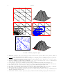
Figure 1. Reference and arbitrary 2- and 3-simplex elements, and a global (2D) basis function.
where
(3.4)
< F (u), v >=
Z
a(x)(∇[u + uD ]) · ∇v + b(x, [u + uD ])v dx.
Ω
The bilinear linearization form < DF (u)w, v > in the case of the PE is again produced as the Gateaux
derivative of the nonlinear form < F (u), v > above:
Z d
∂b
< DF (u)w, v >=
< F (u + tw), v >
(x, u + uD )wv dx.
=
a(x)∇w · ∇v +
dt
∂u
t=0
Ω
4. Multilevel adaptive finite element methods
4.1. The finite element method for nonlinear elliptic equations. A Petrov-Galerkin approximation
of the solution to (2.8) is the solution to the following subspace problem:
(4.1)
1
1
,
Find uh ∈ Uh ⊂ H0,D
such that < F (uh ), vh > = 0, ∀vh ∈ Vh ⊂ H0,D
1
for some chosen subspaces Uh and Vh of H0,D
(Ω). A finite element method is simply a Petrov-Galerkin
approximation method in which the subspaces Uh and Vh are chosen to have the extremely simple form
of continuous piecewise low-degree polynomials with local support, defined over a disjoint covering of the
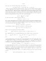
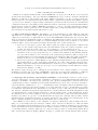
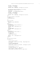
domain Ω by elements, typically simple polyhedra. For example, in the case of continuous piecewise linear
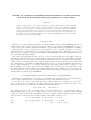
polynomials defined over a disjoint covering with 2- or 3-simplices (cf. Figure 1), the basis functions are
easily defined element-wise using the unit 2-simplex (triangle) and unit 3-simplex (tetrahedron) as follows:
φ̃0 (x̃, ỹ)
φ̃1 (x̃, ỹ)
φ̃2 (x̃, ỹ)
= 1 − x̃ − ỹ
= x̃
= ỹ
φ̃0 (x̃, ỹ, z̃)
φ̃1 (x̃, ỹ, z̃)
φ̃2 (x̃, ỹ, z̃)
φ̃3 (x̃, ỹ, z̃)
=
=
=
=
1 − x̃ − ỹ − z̃
ỹ
x̃
z̃
For a simplex mesh with n vertices, a set of n global basis functions {φi (x, y, z), i = 1, . . . , n} are defined, as
in the right-most picture in Figure 1, by combining the support regions around a given vertex, and extending
the unit simplex basis functions to each arbitrary simplex using (affine) coordinate transformations.
The above basis functions clearly do not form any subspace of C 2 (Ω), the space of twice continuously
differentiable functions on Ω, which is the natural function space in which to look for the solutions to second
order elliptic equations written in the strong form, such as equation (2.1). This is due to the fact that they
are discontinuous along simplex faces and simplex vertices in the disjoint simplex covering of Ω. However,
one can show that in fact [20]:
1
Vh = span{φ1 , . . . , φn } ⊂ H0,D
(Ω), Ω ⊂ Rd ,
so that these continuous, piecewise defined, low-order polynomial spaces do in fact form a subspace of
the solution space to the weak formulation of the problems we are considering here. Taking then U h =
MCLITE: AN ADAPTIVE MULTILEVEL FINITE ELEMENT MATLAB PACKAGE
5
span{φ1 , φ2 , . . . , φn }, Vh = span{ψ1 , ψ2 , . . . , ψn }, equation (4.1) reduces to a set of n nonlinear algebraic
relations (implicitly defined) for n coefficients {αk } in the expansion
uh =
n
X
α k φk .
k=1
In particular, regardless of the complexity of the form < F (u), v >, as long as we can evaluate it for given
arguments u and v, then we can evaluate the nonlinear discrete residual of the finite element approximation
uh as:
n
X
ri =< F (
αk φk ), ψi >, i = 1, . . . , n.
k=1
Since the form < F (u), v > involves an integral in this setting, if we employ quadrature then we can simply
sample the integrand at quadrature points; this is a standard technique in finite element technology. Given
the
Pn local support nature of the functions φk and ψi , all but a small constant number of terms in the sum
k=1 αk φk are zero at a particular spatial point in the domain, so that the residual r i is inexpensive to
evaluate when quadrature is employed. In many cases, the discrete polynomial “test” subspace is taken to
be the same as the solution space, or Vh ≡ Uh , in which case the method is referred to as a Galerkin rather
than a Petrov-Galerkin method.
The two primary issues in applying this approximation method are then:
(1) The approximation error ku − uh kX , for various norms X,
(2) The computational complexity of solving the n algebraic equations.
The first of these issues represents the core of finite element approximation theory, which itself rests on the
results of classical approximation theory. Classical references to both topics include [20, 23, 21]. The second
issue is addressed by the complexity theory of direct and iterative solution methods for sparse systems of
linear and nonlinear algebraic equations, cf. [28, 42].
4.2. Error estimation, adaptive simplex subdivision, and conformity. A priori error analysis for the
finite element method for addressing the first issue is now a well-understood subject [19, 20]. Much activity
has recently been centered around a posteriori error estimation, and its use in adaptive mesh refinement
algorithms [4, 3, 6, 43, 44, 45]. These estimators include weak and strong residual-based estimators [4, 3, 43],
as well as estimators based on the solution of local problems [11, 13]. The challenge for a numerical method
is to be as efficient as possible, and a posteriori estimates are a basic tool in deciding which parts of the
solution require additional attention. While the majority of the work on a posteriori estimates has been for
linear problems, nonlinear extensions are possible through linearization theorems (cf. [43, 44]). The solveestimate-refine structure in MCLite (similar to that in MC) exploiting these a posteriori estimators is as
follows:
Algorithm 4.1. (Adaptive multilevel finite finite element approximation)
• While (ku − uh kX > T OL) do:
(1) Find uh ∈ Uh such that < F (uh ), vh >= 0, ∀vh ∈ Vh
(2) Estimate ku − uh kX over each element, set Q1 = Q2 = ∅.
(3) Place simplices with large error in “refinement” Q1
(4) Bisect all simplices in Q1 (removing them from Q1),
and place any nonconforming simplices created in Q2.
(5) Q1 is now empty; set Q1 = Q2, Q2 = ∅.
(6) If Q1 is not empty, goto (4).
• end while
The conformity loop (4)–(6), required to produce a globally “conforming” mesh (described below) at the
end of a refinement step, is guaranteed to terminate in a finite number of steps (cf. [38, 39]), so that the
refinements remain local. Element shape is crucial for approximation quality; the bisection procedure in
step (4) is guaranteed to produce nondegenerate families if the longest edge is bisected is used in 2D [40, 41],
and if marking or homogeneity methods are used in 3D [2, 15, 14, 32, 35, 37]. Whether longest edge bisection
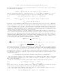
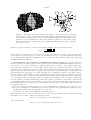
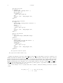
is nondegenerate in 3D apparently remains an open question. Figure 2 shows a single subdivision of a 2simplex or a 3-simplex using either 4-section (first figure from left), 8-section (fourth figure from left), or
bisection (third and sixth figures from left). The paired triangle in the 2-simplex case of Figure 2 illustrates
6
M. HOLST
Subdividing 2-simplices (triangles)
Subdividing 3-simplices (tetrahedra)
Figure 2. Refinement of 2- and 3-simplices using 4-section, 8-section, and bisection.
the nature of conformity and its violation during refinement. A globally conforming simplex mesh is defined
as a collection of simplices which meet only at vertices and faces; for example, removing the dotted bisection
in the third figure from the left in Figure 2 produces a non-conforming mesh. Non-conforming simplex meshes
create several theoretical as well as practical implementation difficulties, and the algorithms in MCLite (as
well as those in MC [29] and PLTMG [6], and similar simplex-based adaptive codes [29, 37, 17, 18, 16])
enforce conformity using the above finite queue swapping strategy or a similar approach.
4.3. Inexact-Newton methods and linear multilevel methods. Addressing the complexity of Step 1
of the algorithm above, Newton methods are often the most effective:
Algorithm 4.2. (Damped-inexact-Newton)
• Given an initial u
• While (| < F (u), v > | > T OL ∀v) do:
(1) Find w such that < DF (u)w, v >= − < F (u), v > +r, ∀v
(2) Set u = u + αw
• end while
The bilinear form < DF (u)w, v > in the algorithm above is the (Gateaux) linearization of the nonlinear
form < F (u), v >, defined earlier. This form is easily computed from most nonlinear forms < F (u), v >
which arise from second order nonlinear elliptic problems. The possibly nonzero “residual” term r is to allow
for inexactness in the Jacobian solve for efficiency, which is quite effective in many cases; cf. [10, 22, 24].
The parameter α brings robustness to the algorithm [8, 9, 24]. If folds or bifurcations are present, then the
iteration is modified to incorporate path-following [7, 30].
As was the case for the nonlinear residual < F (·), · >, the matrix representing the bilinear form in the
Newton iteration is easily assembled, regardless
of the complexity of the bilinear form < DF (·)·, · >. In
Pn
particular, the matrix equation for w = j=1 βj φj has the form:
AU = F,
where
Aij =< DF (
n
X
k=1
αk φk )φj , ψi >,
Fi =< F (
n
X
αk φk ), ψi >,
U i = βi .
k=1
As long as the integral-based forms < F (·), · > and < DF (·)·, · > can be evaluated at individual points in
the domain, then quadrature can be used to build the Newton equations, regardless of the complexity of the
forms. This is one of the most powerful features of the finite element method, and is exploited to an extreme
in the code MCLite and MC (see [29]).
It can be shown that the Newton iteration above is dominated by the computational complexity of solving
the n linear algebraic equations in each iteration; cf. [10, 26]. We use MATLAB’s builtin sparse direct solver
in MCLite for the solution of these equations, which is know to have complexity of O(n 1.5 ) for model problems
in two dimensions. However, the complexity of sparse direct methods decays to O(n 2 ) in three dimensions,
and as a result we employ algebraic multilevel methods in the MC implementation (cf. [29]).
MCLITE: AN ADAPTIVE MULTILEVEL FINITE ELEMENT MATLAB PACKAGE
7
5. The computer program MCLite
MCLite is an adaptive multilevel finite element MATLAB code developed by M. Holst over several years
at Caltech and UC San Diego. It is a two-dimensional MATLAB prototype of the two- and three-dimensional
ANSI-C code MC [29, 5], also written by M. Holst. MCLite is designed to produce provably accurate numerical solutions to two-dimensional scalar nonlinear elliptic equations in an efficient way. MCLite employs
a posteriori error estimation, adaptive simplex subdivision, global inexact-Newton methods, and numerical
continuation methods, for the highly accurate numerical solution of this class of problems. The MC ANSI-C
implementation extends the MCLite MATLAB capabilities to both two- and three-dimensional nonlinear
elliptic systems of tensor equations on two- and three-manifolds, by employing unstructured algebraic multilevel methods for the linear systems which arise; cf. [29].
5.1. The overall design of MCLite. The MCLite code is an implementation of Algorithm 4.1, employing
Algorithm 4.2 for nonlinear elliptic equations that arise in Step 1 of Algorithm 4.1. The linear Newton
equations in each iteration of Algorithm 4.2 are solved with MATLAB’s builtin sparse direct solvers. The
Newton equations are supplemented with a continuation algorithm when necessary. Several of the features
of MCLite, which are inherited from MC, are somewhat unusual, allowing for the treatment of very general
nonlinear elliptic operators and general domains. In particular, some of these features are:
• Abstraction of the elliptic equation: The elliptic equation is defined only through a nonlinear weak
form over the domain, along with an associated linearization form, also defined everywhere on the
domain. (precisely the forms < F (u), v > and < DF (u)w, v > in the discussions above).
• Abstraction of the domain manifold: The domain manifold is specified by giving a polyhedral representation of the topology, along with a set of coordinate labels. MCLite works primarily with the
topology of the domain (i.e., the connectivity of the polyhedral representation). The geometry of the
domain manifold is provided primarily through the form definitions. (MC carries this a bit further,
allowing for the use of 2- and 3-manifolds with multiple coordinate systems as PDE domains.)
• Dimension-independence: While MCLite is a two-dimensional implementation, all of the algorithms
extend immediately to three (and higher) dimensions. To achieve this dimension-independence,
MCLite employs the simplex as its fundamental geometrical object for defining finite element bases.
(This allows MCLite to be used as a prototype code for trying things out that will later be implemented in the ANSI-C code MC.)
The abstract weak form approach to defining the problem allows for the complete definition of a problem
in MCLite by writing only a few lines of MATLAB to define the two weak forms. Changing to a different
problem involves providing only a different definition of the forms and a different domain description.
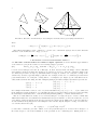
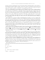
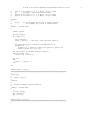
5.2. Topology and geometry representation in MCLite. A datastructure referred to as the ringedvertex (cf. [29]) is used to represent meshes of d-simplices of arbitrary topology. This datastructure, illustrated
in Figure 3, is similar to the winged-edge, quad-edge, and edge-facet datastructures commonly used in the
computational geometry community for representing 2-manifolds [36], but it can be used more generally to
represent arbitrary d-manifolds, d = 2, 3, . . .. It maintains a mesh of d-simplices with near minimal storage,
yet for shape-regular (non-degenerate) meshes, it provides O(1)-time access to all information necessary
for refinement, un-refinement, and discretization of an elliptic operator. The ringed-vertex datastructure
also allows for dimension-independent implementations of mesh refinement and mesh manipulation, with
one implementation covering arbitrary dimension d. An interesting feature of this datastructure is that
the structures used for vertices, simplices, and edges are all of fixed size, so that a fast array-based implementation is possible, as opposed to a less-efficient list-based approach commonly taken for finite element
implementations on unstructured meshes. A detailed description of the ringed-vertex datastructure, along
with a complexity analysis of various traversal algorithms, can be found in [29].
Since MCLite is based entirely on the d-simplex, for adaptive refinement it employs simplex bisection,
using one of the simplex bisection strategies outlined earlier. Bisection is first used to refine an initial
subset of the simplices in the mesh (selected according to some error estimates, discussed below), and then a
closure algorithm is performed in which bisection is used recursively on any non-conforming simplices, until
a conforming mesh is obtained (outlined above). If it is necessary to improve element shape (which effects
finite element approximation quality), MCLite attempts to optimize the following simplex shape measure
8
M. HOLST
Figure 3. Polyhedral mesh representation. The figure on the left shows the overlapping
support regions of two vertex-based global basis functions. The polyhedral mesh topology
is represented by MCLite using a ringed vertex datastructure illustrated in the figure on the
right; the topology primitives are vertices and d-simplices. (Edges are temporarily created
during subdivision, but are then destroyed; a similar ring datastructure is used to represent
the edge topology.)
function for a given d-simplex s, in an iterative fashion, similar to the approach taken in [12]:
1
22(1− d ) 3
η(s, d) = P
d−1
2
2
|s| d
2
0≤i<j≤d |eij |
The quantity |s| represents the (possibly negative) volume of the d-simplex s, and |e ij | represents the length
of the edge that connects vertex i to vertex j in the simplex. For d = 2, this is the shape-measure used
in [12], with a slightly different normalization. For d = 3, this is the shape-measure given in [31], again with
a slightly different normalization.
5.3. Discretization, error estimation, and adaptivity in MCLite. MCLite uses piecewise linear elements to discretize the elliptic equation, The equations is the solved using MATLAB’s builtin sparse direct
solver, and a posteriori error estimates are computed from the discrete solution to drive adaptive mesh refinement. The idea of adaptive error control in finite element methods is to estimate the behavior of the actual
solution to the problem using only a previously computed numerical solution, and then use the estimate to
build an improved numerical solution by upping the polynomial order (p-refinement) or refining the mesh
(h-refinement) where appropriate. Note that this approach to adapting the mesh (or polynomial order) to
the local solution behavior affects not only approximation quality, but also solution complexity: if a target
solution accuracy can be obtained with fewer mesh points by their judicious placement in the domain, the
cost of solving the discrete equations is reduced (sometimes dramatically) because the number of unknowns
is reduced (again, sometimes dramatically). Generally speaking, if an elliptic equation has a solution with
local singular behavior, such as would result from the presence point loads (delta functions) in the forcing
function (right hand side of equation (2.1)), then adaptive methods tend to give dramatic improvements over
non-adaptive methods.
There are several approaches to adaptive error control, although the following two approaches based on a
posteriori error estimation are usually the most effective (and are in fact equivalent in a certain sense [43]):
(1) Residual estimates (strong and weak) [33, 34, 43, 44]
(2) Solution of local problems (Dirichlet or Neumann) [13, 11]
Most existing work on a posteriori estimates has been for linear problems; nonlinear extensions through
linearization. For example, consider the nonlinear problem:
F (u) = 0, F ∈ C 1 (X, Y ∗ ), X, Y Banach spaces,
and a discretization:
Fh (uh ) = 0, Fh ∈ C 0 (Xh , Yh∗ ), Xh ⊂ X, Yh ⊂ Y.
MCLITE: AN ADAPTIVE MULTILEVEL FINITE ELEMENT MATLAB PACKAGE
9
Nonlinear residuals F (uh ) can be used to estimate the error ku − uh kX , using linearization theorems; here
is an example of such a theorem due to Verürth [43].
Theorem 5.1. Let u ∈ X be a regular solution of F (u) = 0, so that DF (u) is a linear homeomorphism of
X onto Y ∗ . Assume DF is Lipschitz continuous at u, so that there exists R0 such that
kDF (u) − DF (uh )kL(X,Y ∗ )
γ=
sup
< ∞.
ku − uh kX
uh ∈B(u,R0 )
Let R = min{R0 , γ −1 kDF (u)−1 kL(Y ∗ ,X) , 2γ −1 kDF (u)kL(X,Y ∗ ) } Then, for all uh ∈ B(u, R),
1
−1
kDF (u)kL(X,Y ∗ ) · kF (uh )kY ∗ ≤ ku − uh kX ≤ 2kDF (u)−1 kL(Y ∗ ,X) · kF (uh )kY ∗
2
The effect of linearization is swept under the rug somewhat by the choice of R sufficiently small. However,
since we typically construct highly refined meshes where needed, such local linear estimates are reasonable.
Note that kF (uh )kY ∗ can be estimated in several ways, including
(1) Approximation by kFh (uh )kY ∗
(2) Solution of local problems
The two approaches are often equivalent up to constants. For reasons of efficiency in the case of elliptic
systems in spatial dimension three, we employ the first approach in MC, referred to as estimation by strong
residuals. In MCLite, the error estimator is user-specified; the user is given all of the information about
an element and the current discrete solution in the element, and is asked to produce an error estimate for
the element. This can be as simple as computing the average of the jumps in the normal derivatives of the
solution gradient across the edges shared with neighboring elements, or the complete calculation of a bound
on the strong form of the residual [43]. In particular, one employs the linearization theorem above, together
with some derived (but computable) upper and lower bounds on the nonlinear residual kF (uh )kY ∗ given by
the following pair of inequalities:
A ≤ kF (uh )kY ∗ ≤ B.
There exact forms of A and B, and their efficient calculation, is quite problem dependent in the nonlinear
case; cf. [43].
5.4. Solution of of linear and nonlinear systems with MCLite. When a system of nonlinear finite
element equations must be solved in MCLite, the global inexact-Newton Algorithm 4.2 is employed, where
the linearization systems are solved by MATLAB’s builtin sparse direct solver. When necessary, the Newton
procedure in Algorithm 4.2 is supplemented with a user-defined normalization equation for performing an
augmented system continuation algorithm. Coupled with the superlinear convergence properties of the outer
inexact Newton iteration in Algorithm 4.2, this leads to an overall complexity of O(N 1.5 ) for the solution of
the discrete nonlinear problems in Step 1 of Algorithm 4.1. Combining this low-complexity solver with the
judicious placement of unknowns only where needed due to the error estimation in Step 2 and the subdivision
algorithm in Steps 3-6 of Algorithm 4.1, leads to an effective low-complexity approximation technique for
solving this general class of elliptic problems.
6. Availability of MCLite
MCLite and various supporting tools are available under the GNU copyleft license, and may be found at
the following website:
http://www.scicomp.ucsd.edu/~mholst/codes/mclite/
Appendix: Actually Using MCLite
Here are is a brief description of all routines in the package; this information is also contained in the
README file distributed with the package.
% documentation files
file README
# THIS FILE -- description of the package
file COPYING
# the GNU license which governs package distribution
file QUICKSTART
# if you have no patience
10
M. HOLST
% primary controlling routines
file go.m
# main MCLite driver program
file assem.m
# assemble the discrete system
file newton.m
# solve the discrete system with newton’s method
file mastr.m
# get master element information
file read.m
# read in a mesh from a standard "MCSF" mesh file
file write.m
# write out a mesh to a standard "MCSF" mesh file
file writemcs.m
# low-level routine to write an "MCSF" mesh file
file writemce.m
# low-level routine to write an "MCEF" mesh file
file writeoff.m
# write out mesh to standard "OFF" file or socket
file writeoffs.m
# write out solution to standard "OFF" file or socket
file zedgmesh.m
# builds an MCEF mesh by treating a matrix as the graph
file mcin.m
# a sample "MCSF" mesh file (the unit square)
file mcinTOR.m
# a sample "MCSF" mesh file (a torus)
file mcout.m
# a sample "MCSF" mesh file (another torus)
file mcout.off
# a sample "OFF" mesh file
% high-level error
file mark.m
file refin.m
file refinbis.m
file refinqud.m
estimation and refinement routines
# tag simplices for refinement (e.g., error estimation)
# refine a set of marked simplices until conformity
# one pass through simplices, bisecting marked ones
# one pass through simplices, quadrasecting marked ones
% low-level simplex ring manipulation routines
file bldsring.m
# build simplex rings for all simplices in the mesh
file kilring.m
# destroy simplex rings for all simplices in the mesh
file chkmesh.m
# extensive consistency/conformity check of entire mesh
file addsring.m
# add a single simplex to all of its simplex rings
file delsring.m
# delete a single simplex from all of its rings
file sinring.m
# is a particular simplex in a particular simplex ring
file addering.m
# add a single edge to all of its edge rings
file getedge.m
# get the unique edge (if exists) between two vertices
file getnabor.m
# get the unique simplex (if exists) sharing a face
file longedge.m
# determine the longest edge of a single simplex
file vneum.m
# yes/no answer about whether tri/edge/vert is neumann
file vdiri.m
# yes/no answer about whether tri/edge/vert is dirichlet
% misc untilities and plotting tools
file assert.m
# an assertion macro for verifying correctess/debugging
file mypaus.m
# pause until the return key is pressed
file draw1.m
# draw a mesh of vertices and simplices (mode 1)
file draw2.m
# draw a mesh of vertices and simplices (mode 2)
file draw3.m
# draw a mesh of vertices and simplices (mode 3)
file drawf.m
# draw a function over a mesh of vertices and simplices
file u.m
# move the plot up
file d.m
# move the plot down
file r.m
# move the plot right
file l.m
# move the plot left
% problem specification (user-defined)
file fu_v.m
# nonlinear weak form defining the pde
file dfu_wv.m
# linearization bilinear form for the pde
file u_d.m
# dirichlet boundary function
file u_t.m
# optional analytical solution for testing purposes
file edgsplit.m
# user-defined procedure to bisect edges in the mesh
There is usually a very descriptive header block in each MATLAB routine; one can view this documentation
for the routine by either editing the MATLAB routine, or by typing e.g. help read at the MATLAB
MCLITE: AN ADAPTIVE MULTILEVEL FINITE ELEMENT MATLAB PACKAGE
11
prompt to view the documentation for the routine read.m. This documentation will be your best guide to
understanding and using the MCLite package. I stress again: read the documentation in the header blocks
of the routines, and also read the documentation in the code itself; it is quite well-documented throughout
(that is the only way I can write code and expect to understand it the next day!)
The most confusing thing about the MCLite package is usually the ringed vertex datastructure that is
used to represent the simplex mesh. By reading the documentation in the file read.m, you will understand
exactly what the basic datastructure is. The simplex rings are simply linked lists of simplices that begin
at vertices; from any vertex, you can walk this list to find all simplices (triangles in MCLite) which use
that vertex. By using this single structure, you can assemble information such as which simplices are edge
neighbors, and so forth. Similarly, the edge rings are linked lists of edges which begin at vertices; from
any vertex, you can find all edges which use that vertex. By using this single structure, you can assemble
information such as which vertices share edges, and so forth. The routines getnabor.m and sinring.m do
some of these things; again, start reading the documentation in the routines and you will begin to understand
the overall structure.
The routines in the “low-level simplex ring manipulation routines” section above simply build,
destroy, traverse, and manipulate the ringed vertex datastructure (the simplex and edge rings around a
vertex). The actual ring datastructures are built by the routines bldsring.m, addsring.m, and addering.m.
The routine bldsring.m is called just before a mesh is refined in the routine refin.m; bldsring.m simply
calls addsring.m for each simplex, which adds each simplex to the simplex rings that start at each of its
vertices. The routine addering.m adds an edge to the edge rings that start at each of its two vertices.
There are several advantages to using the ringed vertex datastructure; the primary one as far as MCLite is
concerned is that all vertices, edges, and simplices have fixed size, so that an array-based implementation in
MATLAB is possible. (This also makes for a faster ANSI-C implementation in MC, compared to linked lists
of variable-sized datastructures.)
Here are a few additional guidelines and pointers to help you get started. The user tells MCLite about the
particular PDE to solve by specifying the nonlinear weak form in the file fu v.m, along with its linearization
weak form dfu wv.m. (We will look more closely at these two files below.) The user also specifies the Dirichlet
boundary condition function as the function u d.m. The function u t.m is a function that is provided as
a slot for an analytical solution to the PDE for testing purposes, if available (otherwise u t.m can simply
return with no action).
The specification of the domain over which to solve the PDE adaptively is effected by providing a simplex
mesh input file mcin.m in MCSF format, along with a single routine edgsplit.m which tells MCLite how to
bisect edges in the mesh when doing refinement. The exact specification of the MCSF format is described in
detail in the header to the mesh read routine read.m. The edgsplit.m file can be simply the usual bisection
of a line in the plane (the average of the two input points), or it can be more complicated to reflect the
correct refinement of boundary edges, or to allow for the underlying domain to be a 2-manifold (this is done
in a more sophisticated manor in MC to handle tensor equations correctly; cf. [29]).
MCLite is used by beginning a MATLAB session, and then executing the script go.m. This script is a
simple driver that first reads in a mesh in MCSF format (the simplex mesh input file format that MCLite and
MC share), and then goes into the discretize/solve/estimate/refine loop in Algorithm 4.1. The script can be
completely controlled by editing it and changing the various parameters that appear in the “controlling
parameters” section of the driver. Along with the PDE and mesh specification routines described above,
the MCLite package can be used simply by editing and running go.m.
The go.m file is listed below:
%%%%%%%%%%%%%%%%%%%%%%%%%%%%%%%%%%%%%%%%%%%%%%%%%%%%%%%%%%%%%%%%%%%%%%%%%%%%%%
%
% Prototype:
%
%
None (script)
%
% Purpose:
%
%
Driver script for MCLite package.
%
% Author:
Michael Holst
12
M. HOLST
%
%%% some i/o
clc;
% clf;
fprintf(’\n’);
fprintf(’-------------------------------------------------------------\n’);
fprintf(’MCLite version 1.0, Copyright (C) 1998 Michael Holst\n’);
fprintf(’This is free software, and you are welcome to redistribute it\n’);
fprintf(’under certain conditions; see the file "COPYING" for details.\n’);
fprintf(’Note that MCLite comes with ABSOLUTELY NO WARRANTY.\n’);
fprintf(’\n’);
fprintf(’For MCLite documentation: In MATLAB, type "help filename".\n’);
fprintf(’-------------------------------------------------------------\n’);
fprintf(’\n’);
fprintf(’MAIN: STARTING: MCLite (MC-Lite) Code\n’);
%%% controlling parameters
levels
refkey
estkey
solkey
chkkey
=
=
=
=
=
23;
1;
1;
1;
0;
%%%
%%%
%%%
%%%
%%%
num of refinements plus one
refinement type (0=bisection,1=quadrasection)
estimator (0=mark all,1=geometric,2=a posteriori)
solve key (0=no, 1=yes)
conformity check the mesh (0=no,1=yes--check is slow)
iplotMan
iplotMesh
igraphA
ispyA
iplotSol
igenPS
=
=
=
=
=
=
1;
1;
1;
1;
1;
1;
%%%
%%%
%%%
%%%
%%%
%%%
MATLAB
MATLAB
MATLAB
MATLAB
MATLAB
MATLAB
gv
gvs
socktype
= 0;
= 0;
= 0;
plot of manifold mesh (0=none,1=manifold)
plot of mesh (0=none,1=mesh)
graph of matrix (0=none,1=graph)
spy of matrix (0=none,1=spy)
plot of solution (0=none,1=soln)
generate postscript (0=no,1=yes)
%%% MCgl or Geomview plot of manifold mesh (0=none,1=yes)
%%% MCgl or Geomview plot of solution mesh (0=none,1=yes)
%%% UNIX domain or INET sockets (0=UNIX domain, 1=INET)
%%% construct operators for the nested sequence of spaces
for level = 1 : levels
fprintf(’MAIN: -------\n’);
fprintf(’MAIN: LEVEL %g\n’,level);
fprintf(’MAIN: -------\n’);
if (level == 1)
%%% create the initial coarse mesh
fprintf(’MAIN: defining the mesh..’);
t0 = clock;
[VERT,SIMP] = read(0);
the_time = etime(clock,t0);
[N,eight]
= size(VERT);
[L,seventeen] = size(SIMP);
fprintf(’..done. [N=%g,L=%g] [time=%g]\n’,N,L,the_time);
else
%%% error estimate and the mark mesh (some uniform refinements first)
fprintf(’MAIN: marking the mesh..’);
t0 = clock;
[SIMP,QUE]
= mark(VERT,SIMP,estkey);
MCLITE: AN ADAPTIVE MULTILEVEL FINITE ELEMENT MATLAB PACKAGE
the_time = etime(clock,t0);
[N,eight]
= size(VERT);
[L,seventeen] = size(SIMP);
fprintf(’..done. [N=%g,L=%g]
[time=%g]\n’,N,L,the_time);
%%% adaptively refine the mesh based on the marking
fprintf(’MAIN: refining the mesh..’);
t0 = clock;
[VERT,SIMP]
= refin(VERT,SIMP,QUE,refkey);
the_time = etime(clock,t0);
[N,eight]
= size(VERT);
[L,seventeen] = size(SIMP);
fprintf(’..done. [N=%g,L=%g] [time=%g]\n’,N,L,the_time);
end;
%%% check the mesh for "correctness"
if (chkkey > 0)
chkmesh(VERT,SIMP);
end
%%% plot the mesh
if (gv > 0)
writeoff(socktype,2,VERT,SIMP);
mypaus;
end;
if (iplotMan > 0)
fprintf(’MAIN: plotting the manifold..’);
draw1(VERT,SIMP);
fprintf(’..done. [N=%g,L=%g]\n’,N,L);
mypaus;
draw2(VERT,SIMP);
fprintf(’..done. [N=%g,L=%g]\n’,N,L);
mypaus;
end;
if (iplotMesh > 0)
fprintf(’MAIN: plotting the mesh..’);
draw3(VERT,SIMP);
if (igenPS > 0)
print -depsc mesh.eps
end
fprintf(’..done. [N=%g,L=%g]\n’,N,L);
mypaus;
end;
%%% solve discrete system?
if (solkey > 0)
%%% solve discrete system
fprintf(’MAIN: nonlinear solve starting.
t0 = clock;
[U,Ug,A,F]=newton(VERT,SIMP);
the_time = etime(clock,t0);
fprintf(’MAIN: nonlinear solve finished.
[N=%g,L=%g]\n’,N,L);
[time=%g]\n’,the_time);
%%% discretization error test
U_t = zeros(N,1);
U_t(1:N,1) = u_t(VERT(1:N,1), VERT(1:N,2));
error = norm(U_t - (U+Ug)) / norm(U_t);
fprintf(’MAIN: discretization error is = %g\n’,error);
13
14
M. HOLST
%%% graph the matrix
if (igraphA > 0)
fprintf(’MAIN: graphing matrix..’);
gplot(A,VERT,’b’);
if (igenPS > 0)
print -depsc graph.eps
end
fprintf(’..done. [N=%g,L=%g]\n’,N,L);
mypaus;
end;
%%% show matrix structure
if (ispyA > 0)
fprintf(’MAIN: showing nonzero structure..’);
clf; hold off;
spy(A);
if (igenPS > 0)
print -depsc spy.eps
end
fprintf(’..done. [N=%g,L=%g]\n’,N,L);
mypaus;
end;
%%% plot the solution
if (gvs > 0)
writeoffs(socktype,2,VERT,SIMP,(U+Ug));
mypaus;
end;
if (iplotSol > 0)
fprintf(’MAIN: plotting FEM solution..’);
drawf(VERT,SIMP,(U+Ug));
view(30,30);
if (igenPS > 0)
print -depsc sol.eps
end
fprintf(’..done. [N=%g,L=%g]\n’,N,L);
mypaus;
end;
end; %%% solve discrete system
end; %%% solve-estimate-refine loop
Finally, regarding the weak form routines f uv.m and dfu wv.m, with which you specify completely your
PDE (along with the Dirichlet function u d.m): these two routines must return the value of the integrand
in the weak form integral, evaluated at the list of points that are passed into the routines. This is because
MCLite assembles the nonlinear residual and the linearized stiffness matrix using (Gaussian) quadrature.
MCLite assembles all of the elements at once, so that what is passed to the three routines f uv.m, dfu wv.m,
and u d.m is basically the list of all of the quadratures points required to approximate the integrals need to
assemble all of the element matrices at once.
For a clear example of how to specify these three routines, consider the Bratu problem (for constant
a ∈ R):
−∇ · (a∇u) + λeu
= f,
u = 0
in Ω = [0, 1] × [0, 1],
on ∂Ω.
MCLITE: AN ADAPTIVE MULTILEVEL FINITE ELEMENT MATLAB PACKAGE
15
The weak form < F (u), v > is:
< F (u), v >=
Z
(a∇u · ∇v + λeu v − f v) dv,
Ω
and the bilinear linearization form < DF (u)w, v > is:
Z
< DF (u)w, v >=
(a∇w · ∇v + λeu wv) dv.
Ω
2
sin(πx) sin(πy)
If we choose f (x, y) = 2π a sin(πx) sin(πy) + λe
, then the analytical solution to this problem
is u(x, y) = sin(πx) sin(πy). For this problem, The correct specification of the two forms, the Dirichlet
function, and the analytical solution (which is available in this particular case), are as follows:
function [thetam] = fu_v(evalKey, parm, L, xm,ym, u,ux,uy, pr,prx,pry);
%%%%%%%%%%%%%%%%%%%%%%%%%%%%%%%%%%%%%%%%%%%%%%%%%%%%%%%%%%%%%%%%%%%%%%%%%%%%%%
%
% Prototype:
%
%
[thetam] = fu_v(evalKey, parm, L, xm,ym, u,ux,uy, pr,prx,pry);
%
% Purpose:
%
%
Evaluate the nonlinear form by providing the value of the quantity
%
under the integral sign, at a particular quadrature point.
%
%
Because we do this for all of the elements at one time to make things
%
reasonably fast, we pass some arrays around.
%
% Input:
%
%
evalKey
==> area or surface integral
%
L
==> number of elements to do all at once
%
xm(1:L,1) ==> x-coordinates of quadrature points, one per element
%
ym(1:L,1) ==> y-coordinates of quadrature points, one per element
%
u(1:L,1)
==> u, evaluated on master element
%
ux(1:L,1) ==> partial w.r.t. x of u, one per element
%
uy(1:L,1) ==> partial w.r.t. x of u, one per element
%
pr
==> phi(r), evaluated on master element
%
prx(1:L,1) ==> partial w.r.t. x of phi(r), one per element
%
pry(1:L,1) ==> partial w.r.t. x of phi(r), one per element
%
% Output:
%
%
thetam
==> the integrand for the area or surface integral,
%
not including the jacobian of transformation
%
% Author:
Michael Holst
%
lambda = parm(1);
%%% area integral
if (evalKey == 0)
%%% coefficients
atilde = ones(L,1);
%%% source term
utilde(1:L,1) =
ftilde(1:L,1) =
+
% the first order coefficient function
chosen to give (one) analytical solution
sin(pi*xm) .* sin(pi*ym);
(2*pi*pi) * atilde(1:L,1) .* utilde(1:L,1) ...
lambda * exp(utilde(1:L,1));
16
M. HOLST
%%% nonlinear residual of the given FEM function "u"
thetam(1:L,1) = ...
atilde(1:L,1) .* (ux(1:L,1).*prx(1:L,1)+uy(1:L,1).*pry(1:L,1)) ...
+ (lambda * exp(u(1:L,1)) - ftilde(1:L,1)) * pr;
%%% edge integral (for natural boundary condition)
else if (evalKey == 1)
%%% apply appropriate condition based on which boundary we are on
thetam = zeros(L,1);
for k=1:L
if (xm(k) == 0)
thetam(k) = pi*cos(pi*xm(k))*sin(pi*ym(k))*pr;
elseif (xm(k) == 1)
thetam(k) = -pi*cos(pi*xm(k))*sin(pi*ym(k))*pr;
elseif (ym(k) == 0)
thetam(k) = pi*sin(pi*xm(k))*cos(pi*ym(k))*pr;
elseif (ym(k) == 1)
thetam(k) = -pi*sin(pi*xm(k))*cos(pi*ym(k))*pr;
else
thetam(k) = 0;
end
end
%%% error
else
assert( 0, ’fu_v 1’ );
end
end
function [thetam] = dfu_wv(evalKey, parm, L, xm,ym, u,ux,uy, ...
ps,psx,psy, pr,prx,pry);
%%%%%%%%%%%%%%%%%%%%%%%%%%%%%%%%%%%%%%%%%%%%%%%%%%%%%%%%%%%%%%%%%%%%%%%%%%%%%%
%
% Prototype:
%
%
[thetam] = dfu_wv(evalKey, parm, L, xm,ym, u,ux,uy, ...
%
ps,psx,psy, pr,prx,pry);
%
% Purpose:
%
%
Evaluate the bilinear form by providing the value of the quantity
%
under the integral sign, at a particular quadrature point.
%
%
Because we do this for all of the elements at one time to make things
%
reasonably fast, we pass some arrays around.
%
% Input:
%
%
evalKey
==> area or surface integral
%
L
==> number of elements to do all at once
%
xm(1:L,1) ==> x-coordinates of quadrature points, one per element
%
ym(1:L,1) ==> y-coordinates of quadrature points, one per element
%
u(1:L,1)
==> u, evaluated on master element
%
ux(1:L,1) ==> partial w.r.t. x of u, one per element
%
uy(1:L,1) ==> partial w.r.t. x of u, one per element
%
ps
==> phi(s), evaluated on master element
%
psx(1:L,1) ==> partial w.r.t. x of phi(s), one per element
MCLITE: AN ADAPTIVE MULTILEVEL FINITE ELEMENT MATLAB PACKAGE
%
psy(1:L,1) ==> partial w.r.t. x of phi(s), one per element
%
pr
==> phi(r), evaluated on master element
%
prx(1:L,1) ==> partial w.r.t. x of phi(r), one per element
%
pry(1:L,1) ==> partial w.r.t. x of phi(r), one per element
%
% Output:
%
%
thetam
==> the integrand for the area or surface integral,
%
not including the jacobian of transformation
%
% Author:
Michael Holst
%
lambda = parm(1);
%%% area integral
if (evalKey == 0)
%%% coefficients
atilde = ones(L,1);
% the first order coefficient function
%%% linearized operator evaluated at the FEM function "u"
thetam(1:L,1) = ...
atilde(1:L,1) .* (psx(1:L,1).*prx(1:L,1)+psy(1:L,1).*pry(1:L,1)) ...
+ lambda * exp(u(1:L,1)) * ps * pr;
%%% edge integral (for natural boundary condition)
else if (evalKey == 1)
thetam(1:L,1) = zeros(L,1);
%%% error
else
assert( 0, ’dfu_wv 1’ );
end
end
function [gxy] = u_d(x,y);
%%%%%%%%%%%%%%%%%%%%%%%%%%%%%%%%%%%%%%%%%%%%%%%%%%%%%%%%%%%%%%%%%%%%%%%%%%%%%%
%
% Prototype:
%
%
[gxy] = u_d(x,y);
%
% Purpose:
%
%
Essential boundary condition function.
%
% Author:
Michael Holst
%
[L,one] = size(x);
gxy = zeros(L,1);
gxy = u_t(x,y);
function [uxy] = u_t(x,y);
%%%%%%%%%%%%%%%%%%%%%%%%%%%%%%%%%%%%%%%%%%%%%%%%%%%%%%%%%%%%%%%%%%%%%%%%%%%%%%
%
17
18
M. HOLST
% Prototype:
%
%
[uxy] = u_t(x,y);
%
% Purpose:
%
%
True solution (for testing).
%
% Author:
Michael Holst
%
[L,one] = size(x);
uxy = zeros(L,1);
uxy = sin(pi*x) .* sin(pi*y);
To control the adaptivity in MCLite, the user provides an error estimator routine called mark.m. Given
all of the information about an element and the current discrete solution in the element, this routine decides
whether or not the element should be refined in order to reduce the element-wise error. The default mark.m
routine provided with MCLite marks elements for refinement based on a simple geometric condition (if an
element crosses the unit circle, then it is marked for refinement). Placing the error estimator in “user-land”
allows for quite a bit of flexibility for trying out various error indicators.
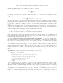
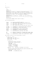
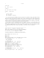
Let’s look at the behavior of MCLite when given the Bratu problem above, over the unit square, and
given the simple geometric element marker as an error estimator. We will look at the I/O produced by
MCLite while it is running, and then will show the graphical output such as the refined meshes, the graph
of the linearized stiffness matrix, the nonzero structure of the matrix, and the plots of the solutions over the
two-dimensional domain. After looking at this example, you should be ready to use MCLite!
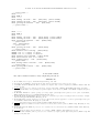
>> go
------------------------------------------------------------MCLite version 1.0, Copyright (C) 1998 Michael Holst
This is free software, and you are welcome to redistribute it
under certain conditions; see the file "COPYING" for details.
Note that MCLite comes with ABSOLUTELY NO WARRANTY.
For MCLite documentation: In MATLAB, type "help filename".
------------------------------------------------------------MAIN: STARTING: MCLite (MC-Lite) Code
MAIN: ------MAIN: LEVEL 1
MAIN: ------MAIN: defining the mesh....done. [N=16,L=18] [time=0.062056]
MAIN: plotting the manifold....done. [N=16,L=18]
--- press return --..done. [N=16,L=18]
--- press return --MAIN: plotting the mesh....done. [N=16,L=18]
--- press return --MAIN: nonlinear solve starting. [N=16,L=18]
NEWTON: iter = 0, ||F(u)|| = 2.54987
NEWTON: iter = 1, ||F(u)|| = 6.67866e-16
MAIN: nonlinear solve finished. [time=0.893346]
MAIN: discretization error is = 0.151521
MAIN: graphing matrix....done. [N=16,L=18]
--- press return --MAIN: showing nonzero structure....done. [N=16,L=18]
--- press return --MAIN: plotting FEM solution....done. [N=16,L=18]
MCLITE: AN ADAPTIVE MULTILEVEL FINITE ELEMENT MATLAB PACKAGE
19
--- press return --MAIN: ------MAIN: LEVEL 2
MAIN: ------MAIN: marking the mesh....done. [N=16,L=18] [time=0.014956]
MAIN: refining the mesh....done. [N=19,L=22] [time=0.153644]
MAIN: plotting the manifold....done. [N=19,L=22]
--- press return --.
.
.
MAIN: ------MAIN: LEVEL 6
MAIN: ------MAIN: marking the mesh....done. [N=117,L=206] [time=0.099601]
MAIN: refining the mesh....done. [N=219,L=406] [time=5.64105]
MAIN: plotting the manifold....done. [N=219,L=406]
--- press return --..done. [N=219,L=406]
--- press return --MAIN: plotting the mesh....done. [N=219,L=406]
--- press return --MAIN: nonlinear solve starting. [N=219,L=406]
NEWTON: iter = 0, ||F(u)|| = 1.91734
NEWTON: iter = 1, ||F(u)|| = 2.9574e-15
MAIN: nonlinear solve finished. [time=3.25056]
MAIN: discretization error is = 0.106009
MAIN: graphing matrix....done. [N=219,L=406]
--- press return --MAIN: showing nonzero structure....done. [N=219,L=406]
--- press return --MAIN: plotting FEM solution....done. [N=219,L=406]
--- press return ---
Acknowledgments
The author thanks R. Bank for many enlightening discussions.
References
1. R. A. Adams, Sobolev spaces, Academic Press, San Diego, CA, 1978.
2. D.N. Arnold, A. Mukherjee, and L. Pouly, Locally adapted tetrahedral meshes using bisection, 1997.
3. I. Babuška and W.C. Rheinboldt, Error estimates for adaptive finite element computations, SIAM J. Numer. Anal. 15
(1978), 736–754.
4.
, A posteriori error estimates for the finite element method, Int. J. Numer. Meth. Engrg. 12 (1978), 1597–1615.
5. R. Bank and M. Holst, A new paradigm for parallel adaptive mesh refinement, SIAM J. Sci. Statist. Comput. (Accepted;
to appear).
6. R. E. Bank, PLTMG: A software package for solving elliptic partial differential equations, users’ guide 8.0, Software,
Environments and Tools, Vol. 5, SIAM, Philadelphia, PA, 1998.
7. R. E. Bank and H. D. Mittelmann, Stepsize selection in continuation procedures and damped Newton’s method, J. Computational and Applied Mathematics 26 (1989), 67–77.
8. R. E. Bank and D. J. Rose, Parameter selection for Newton-like methods applicable to nonlinear partial differential equations, SIAM J. Numer. Anal. 17 (1980), no. 6, 806–822.
, Global Approximate Newton Methods, Numer. Math. 37 (1981), 279–295.
9.
10.
, Analysis of a multilevel iterative method for nonlinear finite element equations, Math. Comp. 39 (1982), no. 160,
453–465.
11. R. E. Bank and R. K. Smith, A posteriori error estimates based on hierarchical bases, SIAM J. Numer. Anal. 30 (1993),
no. 4, 921–935.
12.
, Mesh smoothing using a posteriori error estimates, SIAM J. Numer. Anal. 34 (1997), 979–997.
13. R. E. Bank and A. Weiser, Some a posteriori error estimators for elliptic partial differential equations, Math. Comp. 44
(1985), no. 170, 283–301.
20
M. HOLST
0
20
40
60
80
100
120
140
160
180
200
220
0
20
40
60
80
100
120
nz = 1187
140
160
180
200
220
Figure 4. MCLite graphical output.
14. E. Bänsch, An adaptive finite-element strategy for the three-dimsional time-dependent Navier-Stokes equations, Journal of
Computional and Applied Mathematics 36 (1991), 3–28.
15.
, Local mesh refinement in 2 and 3 dimensions, Impact of Computing in Science and Engineering 3 (1991), 181–191.
16. P. Bastian, K. Birken, K. Johannsen, S. Lang, N. Neuss, H. Rentz-Reichert, and C. Wieners, UG – a flexible software
toolbox for solving partial differential equations, 1998.
17. R. Beck, B. Erdmann, and R. Roitzsch, KASKADE 3.0: An ojbect-oriented adaptive finite element code, Tech. Report
TR95–4, Konrad-Zuse-Zentrum for Informationstechnik, Berlin, 1995.
18. J. Bey, Adaptive grid manager: AGM3D manual, Tech. Report 50, SFB 382, Math. Inst. Univ. Tubingen, 1996.
19. S. C. Brenner and L. R. Scott, The mathematical theory of finite element methods, Springer-Verlag, New York, NY, 1994.
20. P. G. Ciarlet, The finite element method for elliptic problems, North-Holland, New York, NY, 1978.
21. P. J. Davis, Interpolation and approximation, Dover Publications, Inc., New York, NY, 1963.
22. R. S. Dembo, S. C. Eisenstat, and T. Steihaug, Inexact Newton Methods, SIAM J. Numer. Anal. 19 (1982), no. 2, 400–408.
23. R. A. DeVore and G. G. Lorentz, Constructive approximation, Springer-Verlag, New York, NY, 1993.
24. S. C. Eisenstat and H. F. Walker, Globally Convergent Inexact Newton Methods, Tech. report, Dept. of Mathematics and
Statistics, Utah State University, 1992.
25. S. Fucik and A. Kufner, Nonlinear differential equations, Elsevier Scientific Publishing Company, New York, NY, 1980.
MCLITE: AN ADAPTIVE MULTILEVEL FINITE ELEMENT MATLAB PACKAGE
21
26. W. Hackbusch, Multi-grid methods and applications, Springer-Verlag, Berlin, Germany, 1985.
27.
, Elliptic differential equations, Springer-Verlag, Berlin, Germany, 1992.
, Iterative solution of large sparse systems of equations, Springer-Verlag, Berlin, Germany, 1994.
28.
29. M. Holst, Adaptive multilevel finite element methods on manifolds and their implementation in MC, (In preparation;
currently available as a technical report and User’s Guide to the MC software).
30. H. B. Keller, Numerical methods in bifurcation problems, Tata Institute of Fundamental Research, Bombay, India, 1987.
31. A. Liu and B. Joe, Relationship between tetrahedron shape measures, BIT 34 (1994), 268–287.
32.
, Quality local refinement of tetrahedral meshes based on bisection, SIAM J. Sci. Statist. Comput. 16 (1995), no. 6,
1269–1291.
33. J.L. Liu and W.C. Rheinboldt, A posteriori finite element error estimators for indefinite elliptic boundary value problems,
Numer. Funct. Anal. and Optimiz. 15 (1994), no. 3, 335–356.
34.
, A posteriori finite element error estimators for parametrized nonlinear boundary value problems, Numer. Funct.
Anal. and Optimiz. 17 (1996), no. 5, 605–637.
35. J.M. Maubach, Local bisection refinement for N-simplicial grids generated by relection, SIAM J. Sci. Statist. Comput. 16
(1995), no. 1, 210–277.
36. E.P. Mucke, Shapes and implementations in three-dimensional geometry, Ph.D. thesis, Dept. of Computer Science, University of Illinois at Urbana-Champaign, 1993.
37. A. Mukherjee, An adaptive finite element code for elliptic boundary value problems in three dimensions with applications
in numerical relativity, Ph.D. thesis, Dept. of Mathematics, The Pennsylvania State University, 1996.
38. M.C. Rivara, Algorithms for refining triangular grids suitable for adaptive and multigrid techniques, International Journal
for Numerical Methods in Engineering 20 (1984), 745–756.
39.
, Local modification of meshes for adaptive and/or multigrid finite-element methods, Journal of Computational and
Applied Mathematics 36 (1991), 79–89.
40. I.G. Rosenberg and F. Stenger, A lower bound on the angles of triangles constructed by bisecting the longest side, Math.
Comp. 29 (1975), 390–395.
41. M. Stynes, On faster convergence of the bisection method for all triangles, Math. Comp. 35 (1980), 1195–1201.
42. R. S. Varga, Matrix iterative analysis, Prentice-Hall, Englewood Cliffs, NJ, 1962.
43. R. Verfürth, A posteriori error estimates for nonlinear problems. Finite element discretizations of elliptic equations, Math.
Comp. 62 (1994), no. 206, 445–475.
44.
, A review of a posteriori error estimation and adaptive mesh-refinement techniques, John Wiley & Sons Ltd, New
York, NY, 1996.
45. J. Xu and A. Zhou, Local error estimates and parallel adaptive algorithms, 1997, Preprint.
Department of Mathematics, University of California at San Diego, La Jolla, CA 92093, USA.
E-mail address: [email protected]