Download Lab 3

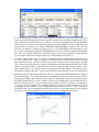
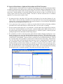
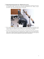
Laboratory 3
Ray Tracing and Monochromatic Aberrations
Physics 4150, last revised 9/17/14
September 17 and 24, 2014
Purpose:
The free educational version of the OSLO lens design program offers full-featured ray tracing and optimization for systems with up to ten optical surfaces. Here you will use it to analyze some of the aberrations
of a single-lens system and a very simple two-lens configuration, and also to model a system of your own
choosing. Similar systems will then be tested in the laboratory to confirm the basic predictions, both quantitative and qualitative, of the analysis. The primary emphasis, though, is on learning to use the ray tracing
software and to understand its output.
Please read Section VIII before undertaking Section IV, and when choosing your custom optical system,
keep in mind that you will need to build and measure it.
Equipment:
1.
2.
3.
4.
5.
6.
7.
8.
9.
10.
11.
12.
13.
14.
Windows-based computers with OSLO ray tracing software, Version 6.5 or higher.
Optical rails with four lens holders.
Bright amber or green LEDs, including one with the plastic focusing lens removed.
White cards or opal glass screens for viewing real images.
He-Ne or diode laser.
Beam expander for He-Ne or diode laser (to at least 2 cm).
Large 20 cm PCX lens, 10–12 cm in diameter.
Large 16.6 cm PCX lens
Pairs of identical 4 cm PCX lenses, 2.5 cm in diameter.
Apertures or irises, with diameters of ¼”, 1 cm and 2 cm.
Round opaque dots, ¼” in diameter.
Point Grey Firefly MV video camera and a computer with NI Vision software. Full data
on the cameras is available on the Physics 4150 web page under “Resources”.
Mounted 20 micron and 50 micron pinholes.
Rulers and meter sticks.
1
I. Ray tracing for an off-axis PCX lens: Coma and Astigmatism
This section introduces the basics of the OSLO lens design program by means of a modified version of
the “cookbook” exercise that starts on p. 34 of the “Optics Reference” book (2011 edition) that serves as
the user’s manual. Here we will define a 20 cm PCX lens and use it to image a bundle of parallel rays
entering at an angle of 25 degrees. Under these conditions several aberrations are present, among which
the most evident are field curvature, coma, and astigmatism.
An excellent discussion of the principles of ray tracing is provided in Chapter 6 of the Optics Reference,
and will not be repeated here. There is also an extended discussion in Hecht, Section 6.2, although he
concentrates exclusively on meridional rays, those that are within the plane of the optical axis. The OSLO
program has no such limitations. In fact, it can deal with diffraction as well as geometric ray tracing,
although we will confine ourselves to geometric optics for now.
If you have trouble following the brief step-by-step instructions below, consult the more extended discussion in the Optics Reference or ask your instructor for help.
1. To get started, Select File/New Lens in the main toolbar. In the “File new” popup box that now appears,
type “PCX 20 cm” or an expression of your choosing for the file name, and change the number of
surfaces to 3 (two lens surfaces plus an aperture stop). Click on ‘OK’. Now we will need to define the
various surfaces, which are defined from left to right as shown in this figure of a generic system (not
the one we study here) from the Optics Reference:
2. In the Surface Data spreadsheet that pops up next, we need to change many of the defaults. In the next
three steps we will modify it to look like the image below. The top window can be used to type entries
that will be transferred to a selected cell lower in the spreadsheet, much as in an Excel spreadsheet. To
start, change the Lens field to match the file name you chose above---it is not required that they be
identical, but it’s appropriate here. Now click on the ‘Gen’ button and set the units to cm (you need to
click on the green check mark to accept the change). Next, change the Entrance beam radius from 1 to
2, and the Field angle to 25 (degrees are the default units). By default the entrance beam is a circular
bundle of parallel rays that are centered around a chief ray, one that passes through the center of the
aperture stop. Change the Primary wavelength to 0.632 microns, which is the wavelength of the laser
that we will use as a light source in the lab. Now go to the row for surface 3, click the button in the
APERTURE RADIUS cell, and click ‘Aperture Stop’. The button at the far left of the row will change
from ‘3’ to ‘AST’ to indicate that this is now the aperture stop of your simple system. Finally, click on
the GLASS button in the row for surface 1, and choose Catalog/Schott/N-BK7 from the cascading
popup menus that will appear. This choice corresponds to ordinary optical crown glass. Click on the
green check mark to accept the entry and return to the main Surface Data spreadsheet.
2
3. You have now defined a lens, but one with no curvature or thickness. Click on the Draw Off button
near the top of the spreadsheet to open the ‘Autodraw’ window that will display a simple sketch of your
setup, which will be updated from now on whenever you change something. Now select the RADIUS
cell of surface 1 and enter 10, the radius that would yield a focal length of 20 cm for a thin PCX lens
with an index of refraction of 1.5. In the APERTURE RADIUS fields for surfaces 1 and 2, enter 6,
since the lens diameter we will use in the lab is 12 cm. In the THICKNESS field for surface 1, enter
2.5 to set the lens thickness, and in the THICKNESS field for surface 2, enter 4 to position the aperture
stop. Now your drawing should show a PCX lens with the curved surface facing left. In the Efl field
you can read the effective focal length of this lens, which should be 19.413079 cm.
4. For surface 3 (the aperture stop), we will use a calculated thickness so that the image plane will wind
up at the paraxial focus. Start by clicking on the button in the THICKNESS cell and selecting
Solves/Axial ray height. Accept the default value of zero in the data entry popup box by selecting
‘OK’. Now force the aperture stop to appear on the drawing: click the button in the SPECIAL cell for
surface 3 and choose Surface Control/General in the new spreadsheet that appears, click the ‘Automatic’ button in the 5th row, and select Drawn on the pop-up menu that appears. Then click the green
checkmark to complete the entry. Your drawing should now show the aperture stop with a dotted line
5. Repeat the same procedure for the SPECIAL cell in row 4 (but not the THICKNESS cell) to complete
the basic lens design. Your drawing should now automatically extend to include the image plane for
paraxial rays. Because some of the off-axis rays miss the image plane, extend it by entering 14 cm for
the APERTURE RADIUS of surface 4 (IMS). There’s just one final thing to do: the lens needs to be
shifted vertically so the 25 rays aren’t quite so far off center. Do this by selecting ‘C’ in addition to
‘F’ for row 3 (AST), bringing up the “Coordinate Data” box. Enter a vertical decentration of 2.4 cm
by changing the value of DCY. Your finished drawing should appear as below. Click on the green
check mark to save your spreadsheet and use File/Save Lens As on the main toolbar to save the design
in a lens file, selecting an appropriate directory to store your work rather than the default.
3
6. Now move on to a full-powered drawing window, as opposed to the simplified auto-updating “Autodraw” window. Select Lens/Lens Drawing/System and accept the defaults in the popup box. If the
resulting drawing has no toolbar, right-click in the drawing area and select ‘Restore Toolbar’. Numerous drawing tools are available. We will use a few of them to determine the shape and size of the
aberrated image spot on the image plane. Click on the ‘Setup window’ button at the upper left, and
select “Spot diagram” if it’s not already checked. Take a look at the various plots of the image spot
that are now available to you. The most useful one for this work is “Plot spot diagram”. Unfortunately
it shows the center spot, not the one for a 25 ray bundle (you can see miniature versions of both by
looking at the “Spot Diagram Analysis” plot). To fix this, right-click in the “Spot Diagram Analysis”
plot area and select ‘Re-calculate using new parameters’. In the new menu that appears, click on the
‘Set object point’ button, then enter 1 for FBY, the fractional Y-coordinate of the object point relative
to the full field. Finally, get rid of all the points for wavelengths other than 0.632  m by returning to
the Surface Data spreadsheet, clicking on ‘wavelength’, and setting the weights to zero for all but the
first wavelength. You should then have a spot diagram similar to this, though with different numbers:
7. Finish by optimizing the lens to make the effective focal length exactly 20 cm and to eliminate Seidel
coma, by adjusting the curvature of surface 1 and the placement of the aperture stop, respectively. You
can directly follow the procedure on pp. 37-40 of the Optics Reference with just one change: for a focal
length of 20 cm, you should optimize the second entry to a value of OCM21-20.0 rather than OCM21100.0. Note that the weights of the two parameters must be set to non-zero values; a good choice is to
set both to 1.0. Run the optimization, and verify by pressing the ‘Abr’ button in the text window that
the Seidel coma, listed as CMA3, is now essentially zero. What is the final radius of curvature for
surface 1? Repeat your Spot Diagram Analysis for this coma-free design, noting the changes, and make
a note of where the aperture should be placed so that you can try it in the lab.
8. Try adjusting the curvature of the image plane to improve the focus of off-axis rays, either by typing
the numbers directly or (much better) by using a slider (see Part II below or p. 41 of the Optics Reference). To make it easier to keep things aligned, reduce the Field angle to 15 degrees and reset the
“decentration” of the aperture to zero (see Part 5). Since the design is coma-free, you should find a
clear vertical line focus and a separate horizontal line focus, with a round image spot halfway between.
To see this, try zooming in on the spot diagram via the right-click menu. For what curvature does the
round spot occur? If you repeat this after moving the aperture to a position for which the coma is large,
you will find it is impossible to get a circular spot for any value of the image plane curvature.
4
II. On-Axis Point Source: Spherical Aberration and Field Curvature
When the object is on the optical axis of a spherical lens imaging system, the only primary aberrations
are spherical aberration (SA) and curvature of the image field, itself due mostly to longitudinal SA. Here
we will examine them with the OSLO lens design program. We will use a PCX lens imaging an on-axis
point source, with the addition of a moveable aperture just after the lens so that we can see the effect of
various regions of the lens when used in isolation. This time we will take somewhat less of a cookbook
approach, so you may need to explore a little.
1. Get started as before, and define a PCX lens with a focal length of 16.6 cm and a diameter of 8 cm.
This is what we will use in the lab. A thickness of 1.2 cm works well. Now set up a narrow beam from
a point source: set the Object (OBJ) radius to 30 cm and its distance to 30 cm (using the THICKNESS
cell), then set the entering beam radius to 0.6 cm.
2. If you want more of the system to be visible in your plots, find the Lens/Lens Drawing conditions
spreadsheet and set the initial distance to the desired value (>30 cm to show everything).
3. Set up an aperture with a radius of 0.5 cm, positioned 1 cm to the right of the second surface of the lens.
Set it up for a calculated thickness just as in part I, so that the image surface (IMS) will always be in
the paraxial image position. Instruct the program that this is a “checked” aperture, so that any rays not
passing through it will be discarded from the image analysis.
4. We would like to be able to slide the aperture back and forth without changing anything else, to see
how the aberrations vary as we look through different portions of the lens. This can be done by rightclicking the button in the SPECIAL cell for the AST column, then selecting Coordinates and entering
a value for DCY “Decentration”. However, there’s a much nicer way to do this interactively: Click on
the “Open the slider-wheel spreadsheet” button on the second line of the main toolbar. Select Surface
3 for one of the sliders, and from the pull-down Item menu, select Y decentration (DCY). Now select
the ‘spot diagram’ button, set the Graphics scale to 1, and select “One Field point” at FBY=0. After
clicking on the green check mark to confirm, you should see a slider bar on the screen plus two drawings, one showing the lens system and the other the spot diagram. You can now use the slider bar to
move the aperture position. After rearranging the windows a little, your screen should look something
like the figure below, in which the aperture is the small vertical line just right of the lens:
5
5. Now determine the predicted shape of the spot when the aperture is centered and also for at least three
off-center positions, like the one shown above. Either print out the spot graphics (use “Plot Spot Diagram” in a graphics window for a full-sized rendition), or carefully record the expected sizes and shapes
for comparison with experimental observations.
III. Ray Tracing for a lens pair: Reducing Spherical Aberration
In lecture, the OSLO program was used to demonstrate that spherical aberration for 1:1 imaging of a
point source can be reduced greatly by reconfiguring a DCX lens into a simple two-lens configuration. The
idea is to cut the DCX lens in half down the center to form two PCX lenses, then to reverse each of them
so that their curved surfaces are almost touching. The improvement occurs because the refraction is distributed almost equally between the four surfaces, minimizing third-order aberrations.
1. Duplicate the configuration demonstrated in lecture by entering the parameters for a pair of PCX lenses
1.25 cm in radius made from BK7 glass. Choose a curvature of 2.07 cm, which should yield a focal
length very close to 4 cm. Start with the flat surfaces touching to form a single composite DCX lens,
as pictured below. Show the ray paths from a point source with an entering beam radius of 0.8 cm.
Note that a “special aperture” has been entered in line 1 of the “Surface Data” table. This will allow us
to study the change in focus as we either use an aperture to pass only paraxial rays, or a round obstruction to block these same rays. In the lab we will investigate this focus shift. In the “Special Aperture
Data” box, create a circular aperture by entering -0.317 cm for x min and y min, and 0.317 cm for x
max and y max. You can now select any of three possibilities for Action: “Pass Thru”, which does
6
nothing, “Transmit,” which gives a conventional aperture, or “Obstruct,” which creates a circular black
dot that absorbs incoming rays near the center of the lens.
2. Starting with the full ray bundle, use the Autofocus tool to find the location of the image plane that
yields a minimum on-axis spot size. How far is it from the position of the paraxial ray focus? Determine and record the minimum rms spot size. Finally, determine and record the calculated spherical
aberration coefficient SA3.
3. Repeat the calculations after setting the “Special Aperture Data” box to define an aperture with a ¼”
diameter (0.317 cm radius), which will transmit only near-paraxial rays. You will need to refocus to
find the new location of the minimum spot size. How much does it move? By how much is the spot
size reduced? Repeat the process again after changing the aperture into an obstruction, so that the
paraxial rays are blocked.
4. Finally, reverse the two lenses so the curved surfaces are nearly touching, and retry the measurements
in items (2) and (3). You will see an obvious improvement both in the drawings and the numbers.
IV. Free-form modeling
Choose a simple optical system, one that you can easily assemble with parts available in the laboratory,
and model it. Next week you will construct and measure the system as Part VIII of this lab. For
example, you might choose to take a pair of 5 cm PCX lenses separated by their focal length, forming
a Ramsden eyepiece, and study the lateral chromatic aberration compared with a single lens. (If you
were to do this, where should the source be located?) As another example, you might use the same
lens pair for “relay imaging” or “f–2f–f imaging,” in which the lenses are separated by distance 2f, and
a source is located at distance f to the left of the first one. How well is a point source reproduced at
distance f to the right of the second lens? How well is an initially well-collimated beam reproduced?
These are just a few examples to set the tone. Feel free to pick any system you wish, so long as it is
simple and can be contructed in the lab.
7
V. Experimental measurements for collimated off-axis rays
1. Set up the scheme modeled in Part I above, using a beam-expanded He-Ne or diode laser as the source
for a parallel ray bundle. The photo shows one possible implementation of this. Initially, set up the
lens on-axis, and verify that the image distance is as expected.
2. Now set the lens and image screen at a 25 degree angle as in part I, keeping the same distance to the
screen as before, and compare the observed image to what you calculated. Some adjustment may be
needed so that the rays enter the lens at the same position for which you did the calculation.
3. Now add an aperture after the lens as shown in the picture, and experiment with the effects of its placement. Can you obtain improvements as predicted in Part I? What seems to be the optimal distance,
and how does it compare with what you predicted for the minimization of coma? (Note: the comparison
may not be very close, since these distortions are rather sensitive to small details.)
8
VI. Experimental measurements for a point source and a single lens
1. As indicated in the photo below, set up the scheme modeled in Part II above, using a bright 594 nm
LED and a 20 micron pinhole as the point source, a 16.6 cm lens, and a Firefly MV camera sensor as
the image plane. Set up a 1 cm diameter aperture about 1 cm behind the lens.
2. Focus the camera with the aperture centered, and determine the actual spot size. Under these conditions, the spot size is limited not only by spherical aberration, but also by the finite size of the pinhole
(20 microns diameter) and the diffraction limit of the 1 cm aperture stop (also about 20 microns). These
three limits can be expected to add roughly in quadrature to give the actual spot size. Compare your
measured value with a prediction on this basis. Note: The OSLO spot reports do not list the relevant
diffraction limit, as they apparently take into account only diffraction by the lens, rather than diffraction
by the aperture stop.
3. Now measure the shape and size of the spot for the same off-axis positions used in Part II. You may
need to increase the source intensity (don’t exceed the maximum marked on your LED!) or increase
the shutter time for the camera in order to obtain a clear image. Compare your results with the calculations.
4. Finally, to give a qualitative but vivid illustration of the effects of spherical aberration, remove the
aperture stop and block the central 2 cm of the lens with a metal or cardboard disk. Note that the outer
portion of the lens is hardly contributing at all to the actual image! Try positioning an image screen or
the camera sensor to determine where the “circle of least confusion” is seen (it should be far in front of
the paraxial image) and about how large it is.
9
VII. Experimental measurements of spherical aberration with two PCX lenses
1. Set up the scheme modeled in Part III by using a pair of 4 cm PCX lenses, 2.5 cm in diameter. It’s
difficult to measure rms spot sizes due to spherical aberration, mainly because the out-of-focus rays
spread over so wide a region that they are difficult to measure. Instead we will concentrate mainly on
the imaging quality. Set up a light box with a back-lit plastic ruler or similar scale, using a variable
transformer so the intensity can be adjusted. To begin, turn the intensity fairly high and use the lenses
to form a real image onto a screen.
2. Starting with the lenses in the “DCX” configuration with the flat surfaces together, set up the lens to
give approximately 1:1 imaging by finding the closest position of the screen for which a clear image
can be obtained. Now add a 1.6–2 cm aperture to approximate the conditions modeled in Part III
above. Compare your observations with what you see using the lenses in the doublet configuration
with the two curved surfaces together. You will probably find that the central part of the image is
sharper and brighter for the doublet, especially with the lens used at full aperture, but you might also
find that distortion is more severe away from the center of the field of view. This is something that we
didn’t model, so it should not come as a total surprise.
3. To be somewhat more quantitative, replace the screen with a Point Grey camera sensor, without a separate camera lens. Turn down the intensity until you get a well-exposed image. Measure the width of
a selected line in your image, the brightness of the background area near the line, and the contrast ratio
(the ratio of the bright background intensity to the dark line, as measured with the line profiling tool).
Compare the “DCX” and doublet configurations without changing any of the camera or source settings,
apart from refocusing the lens and camera positions as necessary to get the best image in each case. If
you have time, try to measure the focus shift when you introduce a ¼” black dot that blocks the paraxial
rays just in front of the lens.
VIII. Evaluating your free-form system
Build whatever you designed in Section IV. Measure whatever you chose as the key parameter to
study. Compare your observations with the modeling, and discuss the level of agreement or disagreement.
10