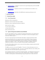
1
ARM TR-016
Microwave Radiometer (MWR) Handbook
August 2006
V. R. Morris
Work supported by the U.S. Department of Energy,
Office of Science, Office of Biological and Environmental Research
August 2006, ARM TR-016
Contents
1
2
3
4
5
6
7
General Overview ............................................................................................................................... 1
Contacts............................................................................................................................................... 1
Deployment Locations and History..................................................................................................... 1
Near-Real-Time Data Plots ................................................................................................................. 2
Data Description and Examples .......................................................................................................... 2
Data Quality ...................................................................................................................................... 11
Instrument Details ............................................................................................................................. 12
Figures
1
Radiometer receiver block diagram .................................................................................................. 13
Tables
1
2
3
4
5
6
7
8
9
10
11
Current Status and Locations .............................................................................................................. 1
Primary Variables................................................................................................................................ 2
Measurement Uncertainties................................................................................................................. 3
Secondary Variables............................................................................................................................ 3
Diagnostic Variables ........................................................................................................................... 3
Data Quality Flags............................................................................................................................... 4
Data Quality Thresholds ..................................................................................................................... 4
Time Quality Flags.............................................................................................................................. 5
Limits for Time ................................................................................................................................... 6
Dimension Variables........................................................................................................................... 6
Instrument Specifications.................................................................................................................. 13
iii
August 2006, ARM TR-016
1. General Overview
The Microwave Radiometer (MWR) provides time-series measurements of column-integrated amounts of
water vapor and liquid water. The instrument itself is essentially a sensitive microwave receiver. That is,
it is tuned to measure the microwave emissions of the vapor and liquid water molecules in the atmosphere
at specific frequencies.
2. Contacts
2.1
Mentor
Marie Cadeddu
Argonne National Laboratory
9700 S. Cass Avenue
Argonne, Illinois 60439
Phone: 630-252-7408
[email protected]
2.2
Instrument Developer
Radiometrics Corporation
2840 Wilderness Place, Unit G
Boulder, Colorado 80301-5414
Phone: 303-449-9192
Fax: 303-786-9343
Website: www.radiometrics.com
3. Deployment Locations and History
Table 1. Current Status and Locations
Serial
Number
Property
Number
Location
4
10
11
12
15
16
17
18
20
21
33
38
WD06605
WD11023
WD14131
WD14132
WD14869
WD13409
WD13410
WD12906
WD24769
WD24770
WD23179
WD30750
SGP/EF14
SGP/CF1
SGP/BF1
SGP/BF5
TWP/CF2
TWP/CF1
TWP/CF3
SGP/BF6
NSA/CF1
NSA/CF2
AMF
SGP/BF4
1
Installation
Date
2004/06/24
1993/12/13
1993/12/13
1993/12/13
1998/11/12
1996/09/23
2002/02/27
1995/06/27
1997/02/28
1999/05/20
2004/09/02
2004/09/02
Status
operational
operational
operational
operational
operational
operational
operational
operational
operational
operational
operational
operational
August 2006, ARM TR-016
4. Near-Real-Time Data Plots
MWR Data Plots.
5. Data Description and Examples
Available data plots and other data products.
5.1
Data File Contents
Datastreams produced by the MWR that are available from the ARM Archive:
•
•
5.1.1
mwrlos - water liquid & vapor along line of sight (LOS) path
mwrtip - brightness temperatures along tipping (TIP) curve airmasses.
Primary Variables and Expected Uncertainty
The MWR receives microwave radiation from the sky at 23.8 GHz and 31.4 GHz. These two frequencies
allow simultaneous determination of water vapor and liquid water burdens along a selected path.
Atmospheric water vapor observations are made at the “hinge point” of the emission line where the vapor
emission does not change with altitude (pressure). Cloud liquid in the atmosphere emits in a continuum
that increases with frequency, dominating the 31.4 GHz observation, whereas water vapor dominates the
23.8-GHz channel. The water vapor and liquid water signals can, therefore, be separated by observing at
these two frequencies.
Table 2. Primary Variables
Variable Name
tbsky23
tbsky31
vap
liq
sky_ir_temp
tbsky23tip
tbsky31tip
vaptip
liqtip
Quantity Measured
23.8 GHz sky brightness temperature
31.4 GHz sky brightness temperature
Total water vapor along LOS path
Total liquid water along LOS path
IR Brightness Temperature
23.8 GHz sky brightness temperature derived from tip curve
31.4 GHz sky brightness temperature derived from tip curve
Total water vapor along zenith path using tip-derived brightness
temperatures
Total liquid water along zenith path using tip-derived brightness
temperatures
2
Unit
K
K
cm
cm
K
K
K
cm
cm
August 2006, ARM TR-016
5.1.1.1
Definition of Uncertainty
Table 3. Measurement Uncertainties
5.1.2
Measurement
Uncertainty
Sky
Blackbody
Blackbody+noise
Gain reference
Receiver gain
Receiver offset
0.018 K
0.12 K
~0.15 K
~0.02 K
~0.09 K
0.035 K
Secondary/Underlying Variables
Table 4. Secondary Variables
Variable Name
time
tnd23
bb23
bbn23
sky23
tnd31
bb31
bbn31
sky31
actaz
actel
tipsky23
tipsky31
tnd23I
tnd31I
5.1.3
Quantity Measured
Unit
Time offset from midnight
Noise injection temp at 23.8 GHz adjusted to tkbb
23.8 GHz Blackbody signal
23.8 GHz blackbody+noise injection signal
23.8 GHz sky signal
Noise injection temp at 31.4 GHz adjusted to tkbb
31.4 GHz Blackbody signal
31.4 GHz blackbody+noise injection signal
31.4 GHz sky signal
Actual Azimuth
Actual elevation angle
23.8 GHz sky signal
31.4 GHz sky signal
Noise injection temp at 23.8 GHz derived from this tip
Noise injection temp at 31.4 GHz derived from this tip
seconds
K
count
count
count
K
count
count
count
deg
deg
count
Count
K
K
Diagnostic Variables
Table 5. Diagnostic Variables
Variable Name
time_offset
tknd
tkxc
tkbb
tkair
wet_window
tnd_nom23
tnd_nom31
Quantity Measured
Time offset from base_time
Noise diode mount temperature
Mixer kinetic (physical) temperature
Blackbody kinetic temperature
Ambient temperature
Water on Teflon window (1=WET, 0=DRY)
Noise injection temp at nominal temperature at 23.8 GHz
Noise injection temp at nominal temperature at 31.4 GHz
3
Unit
seconds
K
K
K
K
unitless
K
K
August 2006, ARM TR-016
Table 5. (cont’d)
Variable Name
tc23
tc31
r23
r31
5.1.4
Quantity Measured
Unit
Temperature correction coefficient at 23.8 GHz
Temperature correction coefficient at 31.4 GHz
23.8 GHz goodness-of-fit coefficient
31.4 GHz goodness-of-fit coefficient
K/K
K/K
unitless
Unitless
Data Quality Flags
Most fields contain a corresponding, sample by sample, automated quality check field in the b1 level
datastreams. These flags are named qc_<fieldname>. For example, the tknd field also has a companion
qc_tknd field. Possible values for each sample of the qc_<fieldname> are shown in the table below.
Table 6. Data Quality Flags
Value
Definition
0
1
2
3
4
5
7
All QC checks passed
Sample contained 'missing data' value
Sample was less than prescribed minimum value
Sample failed both 'missing data' and minimum value checks
Sample greater than prescribed maximum value
Sample failed both minimum and maximum value checks (highly unlikely)
Sample failed minimum, maximum and missing value checks (highly unlikely)
Sample failed delta check (change between this sample and previous sample
exceeds a prescribed value
Sample failed delta and missing data checks
Sample failed minimum and delta checks
Sample failed minimum, delta and missing value checks
Sample failed maximum and delta checks
Sample failed minimum, maximum and delta checks
Sample failed minimum, maximum, delta and missing value checks
8
9
10
11
12
14
15
The minimum and maximum thresholds are currently defined as follows:
Table 7. Data Quality Thresholds
Field
Name
tknd
tkxc
tkbb
tkair
tnd23
Units
K
K
K
K
K
Min
303
303
250
253
163
Max
333
333
320
323
353
4
Delta
N/A
0.5
1
N/A
N/A
August 2006, ARM TR-016
Table 7. (cont’d)
Field
Name
bb23
bbn23
sky23
tbsky23
tnd31
bb31
bbn31
sky31
tbsky31
vap
liq
sky_ir_temp
wet_window
tnd_nom23
tnd_nom31
tc23
tc31
Units
counts
counts
counts
K
K
counts
counts
counts
K
cm
cm
K
unitless
K
K
K/K
K/K
Min
0
0
0
2.73
163
0
0
0
2.73
0.
-3*rms (see note 1)
213
(see note 2)
163
163
N/A
N/A
Max
N/A
N/A
N/A
100
353
N/A
N/A
N/A
100
N/A
N/A
313
N/A
353
353
N/A
N/A
Delta
N/A
N/A
N/A
0.01
N/A
N/A
N/A
N/A
0.01
N/A
N/A
50
N/A
80
80
N/A
N/A
Note 1: rms is liquid_retrieval_rms_accuracy
Note 2: A value of 1 for the wet_window field means that the heater was ON at the time the sample was
taken.
Additional information may be found at MWR Data Object Design for ARM netCDF file header
descriptions.
In addition to the above data quality checks, the qc_time field is also supplied. The purpose of the
qc_time field is to help detect duplicate samples, missing samples or other sample time problems. The
qc_time field contains a value for each sample time. Refer to the table below for details.
Table 8. Time Quality Flags
Value
Description
0
1
2
4
Dt is within specified range
Dt is 0, duplicate sample
Dt is less than specified lower limit
Dt is greater than specified upper limit
5
August 2006, ARM TR-016
Finally, the table below specifies the qc_time limits used for the MWR datastream.
Table 9. Limits for Time
Datastream
Lower
Limit
Upper
Limit
20
39
mwrlos
5.1.5
Dimension Variables
Table 10. Dimension Variables
Variable Name
base_time
lat
lon
alt
5.2
Quantity Measured
Base time in Epoch
north latitude
east longitude
altitude
Unit
seconds
Degrees
degrees
meters above Mean Sea Level
Annotated Examples
This section is not applicable to this instrument.
5.3
User Notes and Known Problems
Positive “spikes” are produced in the measurements during preventative maintenance due to water used to
clean the teflon window.
5.4
Frequently Asked Questions
How should we use the QC flags (qcmin, qcmax, qcdelta)?
Do we disregard suspicious data?
Precipitable water vapor (PWV) and liquid water path (LWP) that exceed the maximum should be
eliminated - these usually indicate rain. PWV below zero is unphysical and arises during rain because of
the opposite signs of the retrieval coefficients. Negative LWP is OK as long as it is within or close to the
RMS uncertainty in the retrieval. The RMS uncertainties in the PWV and LWP are included in the meta
data:
•
•
vapor_retrieval_rms_accuracy[cm] = “0.057881” ; <--for December
liquid_retrieval_rms_accuracy[cm] = “0.003083” ; <--for December.
6
August 2006, ARM TR-016
Why are “qcmax” flags not completely coincident with the weather log reports of rain?
The qcmax flag for liquid is raised when the retrieved liquid water exceeds 1 cm. Such a value is not
possible--it indicates a serious failure of the retrieval, most likely due to water standing on the instrument.
There are two reasons why this may not be completely coincident with weather log reports of rain. First,
the operators are only onsite from 8 am to 5 pm local time at the central facilities; if it rains when the
operators aren’t there, no log entry is made. Second, the problem can arise from standing water, not just
rainfall; there is some time between the end of the rainfall and the evaporation of the water from the
teflon window which covers the mirror on the instrument. So, the operators could report that the rain has
stopped but the microwave radiometer window is still wet and thus still reporting invalid data.
Can we use the data when there are long periods of “qcmin” flags for liquid?
Yes, you can use the data. Actually, liquid values that are negative but within the RMS-accuracy of the
retrieval of zero may be considered equal to zero, which is the physically plausible lower bound.
When the weather log reports fog, is it possible that the microwave window gets covered with dew
and leads to bad data even though no rain is reported?
Dew has a fairly distinct signature - a smooth hump - in the retrieved vapor and liquid as well as in the
underlying brightness temperatures. This is often seen just at or before dawn, however, it usually goes
away before the operators would have reported to the site. (This assessment is borne out by the surface
station data which indicated that the dew point was within the sensor accuracy of the ambient temperature
at about the time when the “hump” first appeared.) For example, on one occasion the operators reported
heavy ground fog at 1400 GMT (8 am local time) and the instrument showed 85-90 microns of liquid. I’d
say the two were consistent.
The instruments are equiped with an “anti-dew” system that is comprised of a continuous fan and a
500-750 W heater controlled by a moisture sensor mounted on top of the instrument. Normally, the fan
blows ambient air over the Teflon window to keep it clear of dust. During condensing or precipitating
conditions the heater turns on to prevent the formation of dew or the settling of fog on the window as well
as to promote the evaporation of rain and snow. The condition of the heater (ON/OFF) is indicated in the
netCDF files by the wet_window variable.
This system seems to work quite well but the sensitivity of the heater needs to be maintained. Because it
is a resistive element, it is somewhat temperature dependent, so it periodically triggers unnecessarily on
cold nights. Although this doesn’t affect the PWV or LWP measurements, it does cause some confusion
when using the wet_window data as an indication of rain or dew or fog.
The MWRs have been retrofitted with new blowers that have greater air flow and heater circuitry that is
less sensitive to ambient temperature.
7
August 2006, ARM TR-016
When should we call the liquid water path zero (i.e. what is the noise level)?
Why do we see significant (+/- 30 g/m3 = +/- 0.03 mm) positive/negative values of the liquid water
path when the sky is clear according to the ceilometer?
The noise level is very low: 0.003 mm = 0.0003 cm RMS. The problem is in the retrieval uncertainty.
Statistical retrieval is essentially a multiple linear regression. Any regression will have a residual error.
In the LWP retrieval the residual error or “theoretical accuracy” is 0.03 mm (RMS), 10 times the
sensitivity or noise limit. So a value of LWP that is +/- 0.03 mm of zero could be clear sky.
The real problem here is that the mean radiating temperature, Tmr, of the atmosphere, which is determined
at the time the retrieval coefficients are computed, is assumed to only vary monthly with the retrieval
coefficients. The truth is that Tmr varies diurnally - enough to cause the zero LWP to vary in a most
annoying fashion within the uncertainty bounds of the retrieval.
How can we correct calibration problems that affect the values of liquid water path?
The retrieval of PWV and LWP is based on a weighted difference of the optical thicknesses of the two
channels. (The weights are the retrieval coefficients.) Because the retrieval coefficients are determined
by linear regression over a climatological range of likely conditions, they implicitly assume the mean
conditions (e.g. mean radiating temperature, mean cloud liquid water temperature in the case of LWP).
The farther the actual conditions are from the mean (due to diurnal and synoptic variations that the
retrieval does not account for), the more error in the retrieval. Clear sky conditions are far from the mean
LWP, and so they have a larger uncertainty than cloudy conditions that may be very close to the average.
Calibration issues aside, the clear sky LWP may be wrong but the cloudy sky LWP may be very close to
correct, so subtracting the clear sky offset from all values of LWP is not an optimal solution.
With respect to calibration errors, the problem is that the calibration value, the “noise injection
temperature” affects the slope of the calibration (K/count) so that an error in the calibration really affects
the scale rather than the offset of the brightness temperatures, but because the retrieved values result from
the difference of the two channels (which are weighted differently) it can look like there is an offset in
LWP for clear sky conditions.
The only good way to fix calibration errors is to reprocess the data to fix the brightness temperatures, then
reapply the retrievals.
What is a reasonable maximum liquid water path?
Suppose the cloud averages 1 g/m3 of liquid water and is 1 km thick. Then the LWP would be
10**-6 g/cm3 x 10**5 cm = 0.1 g/cm2 = 0.1 cm = 1 mm.
Thus, values above, say, 3 mm would be rare; such high values would probably be accompanied by rain
and thus not measured anyway.
8
August 2006, ARM TR-016
Why do we see occasional spikes way over 3 mm in the liquid water path data?
Two events cause the LWP to exceed 1 mm (or 3 mm). The first is rain or melting snow. The second is
condensation (dew). A rule of thumb Ed Westwater (NOAA/ETL) uses is brightness temperatures over
100 K aren’t generally reliable (i.e. the optical depth can’t get that large without precipitation or
condensation on the Teflon window.) This rule is used to set the upper limit for brightness temperatures,
i.e. when the brightness temperatures exceed 100 K, a flag is set in the netCDF data file.
Are the data from the MWRs independent of the radiosondes?
No, not entirely. The retrievals are based on NWS radiosonde data from 1994-1999.
Are the tuning functions still used?
No. Use of the so-called tuning functions was discontinued on 6 April 1996. The tuning functions were
removed from the SGP CF MWR data that were collected between 950101 - 960409. Data collected
before this date have already had these removed by Jim Liljegren, while data after this time window never
had the tuning functions applied.
At the time, it was commonly held that the sondes represented “ground truth” and that the “tuning
functions” (i.e. regressions of model-calculated vs. measured brightness temperatures) accounted for
errors in the microwave absorption model upon which the retrievals were based. Jim Liljegren and
Barry Lesht have since determined that the variation in the sonde calibration explains the differences
between the model calculations and the microwave radiometric measurements. By removing the tuning
functions, the PWV and LWP retrieved from the microwave radiometer are independent of the
radiosondes.
What were the tuning functions?
The tuning functions linearly relate model-calculated microwave brightness temperatures (using
radiosonde data) to brightness temperatures measured with a microwave radiometer. These were needed
to account for imperfections in the microwave absorption model used to develop the retrievals which
relate precipitable water vapor and liquid water path to the microwave brightness temperatures. The
tuning functions should be independent of the instrument and of the location - they should depend only on
the microwave absorption model used in the calculations.
How were the tuning functions determined?
After each sonde launch, the model which computes the integrated vapor from the sonde as well as the
microwave brightness temperatures is run automatically by the data system. Jim Liljegren collected all of
these modeled and measured brightness temperatures between Oct. 92 and Dec. 93, selected those for
which the sky was clear (that is, for which the RMS variation in the liquid-sensing channel brightness
temperature was less than 0.4 K) and calculated a regression for each channel.
9
August 2006, ARM TR-016
What changes were made to the data ingest in October 1998?
The MWR software was revised to provide additional functionality as described below.
1. Faster sampling rate: Standard line-of-sight (LOS) observations can now be acquired at
15-second intervals vs. 20-second intervals previously. (The standard LOS cycle is comprised of
one sky sample per blackbody sample and gain update.)
2. More flexible sampling strategy: Multiple sky observations can be acquired during a LOS cycle,
up to 1024 per gain update. This permits sky samples to be acquired at intervals of 2.67 seconds
for improved temporal resolution of cloud liquid water variations and better coordination with the
millimeter cloud radar during IOPs.
3. Separation of zenith LOS observations from tipping curve (TIP) data: When the radiometer is in
TIP mode, the zenith LOS observations are now extracted, the PWV and LWP computed and
reported separately in the output file. This eliminates the periods of missing LOS data during
calibration checks/updates.
4. Automatic self-calibration: The software now permits the calibration to be updated at specified
intervals or continuously.
To ingest the new format of the raw data, significant changes were made to the MWR Data Object
Design.
Why are there anomalies in the data near local solar noon?
These anomalies are due to the sun in the field of view of the radiometer. They occur near the equinoxes
at TWP around noon in both TIP and LOS modes and at SGP near sunrise and sunset in east-west tip
curve data.
Why are there spikes in the data from November 1999 to July 2002?
The intermittent spikes in the LWP and PWV data were caused by the occurrence of blackbody signals
(in counts) that were half of those expected, yielding negative sky brightness temperatures. This problem
was due to some component of the Windows98 configuration that conflicted with the DOS-based MWR
program or affected the serial port or the contents of the serial port buffer. It was finally corrected by
upgrading the MWR software with a new Windows-compatible program.
10
August 2006, ARM TR-016
6. Data Quality
6.1
Data Quality Health and Status
The following links go to current data quality health and status results.
•
•
DQ HandS (Data Quality Health and Status)
NCVweb for interactive data plotting using.
The tables and graphs shown contain the techniques used by ARM’s data quality analysts, instrument
mentors, and site scientists to monitor and diagnose data quality.
6.2
Data Reviews by Instrument Mentor
Data quality control procedures for this system are mature. On a weekly basis, the instrument mentor
produces and inspects plots of the precipitable water vapor (PWV) and liquid water path (LWP) versus
time. The base level of LWP is evaluated for clear sky episodes and the PWV estimates are compared to
those from the BBSS. DQRs are submitted when needed, and a summary report of data quality is sent
monthly to the SGP site scientist team.
6.3
Data Assessments by Site Scientist/Data Quality Office
All DQ Office and most Site Scientist techniques for checking have been incorporated within DQ HandS
and can be viewed there.
6.4
Value-Added Procedures and Quality Measurement Experiments
Many of the scientific needs of the ARM Program are met through the analysis and processing of existing
data products into “value-added” products or VAPs. Despite extensive instrumentation deployed at the
ARM CART sites, there will always be quantities of interest that are either impractical or impossible to
measure directly or routinely. Physical models using ARM instrument data as inputs are implemented as
VAPs and can help fill some of the unmet measurement needs of the program. Conversely, ARM
produces some VAPs not in order to fill unmet measurement needs, but instead to improve the quality of
existing measurements. In addition, when more than one measurement is available, ARM also produces
“best estimate” VAPs. A special class of VAP called a Quality Measurement Experiment (QME) does
not output geophysical parameters of scientific interest. Rather, a QME adds value to the input
datastreams by providing for continuous assessment of the quality of the input data based on internal
consistency checks, comparisons between independent similar measurements, or comparisons between
measurement with modeled results, and so forth. For more information see, see the VAPs and QMEs web
page and specifically:
•
MWR PROF: Retrievals of water vapor, liquid water, and temperature profiles from a suite of
ground-based instruments.
•
LSSONDE: Radiosonde profiles, where the moisture profile is scaled to match the MWR’s total
precipitable water vapor.
11
August 2006, ARM TR-016
•
QME MWR PROF: Comparisons of retrieved water vapor and temperature profiles from MWR
PROF with radiosonde profiles.
•
QME MWR/LBL: Comparisons of observed versus calculated microwave radiance at two
frequencies.
•
QME MWR COL: Comparisons of the MWR with an instrument performance model.
7. Instrument Details
7.1
7.1.1
Detailed Description
List of Components
Radiometrics WVR-1100 Radiometer
Radiometrics dew blower/heater/rain sensor assembly
Radiometrics tripod or quadrapod and tribrach leveling base
Small form factor computer
AC power cable for radiometer
AC power cable for heater
Serial communications cable
7.1.2
System Configuration and Measurement Methods
The water vapor radiometer receiver is composed of a gaussian optical antenna, a noise diode injection
device, a dual junction isolator, a balanced mixer, an IF amplifier, a detector/video amplifier, and two
Gunn diode oscillators (Figure 1).
The receiver accepts input power from the antenna and supplies a voltage proportional to antenna
temperature (plus antenna noise) via a square law detector to the radiometer voltage-to-frequency
converter on the microprocessor (digital) board. Receiver frequency selection is accomplished by
alternately powering the 23.8 and 31.4 GHz Gunn diode local oscillators. Brightness temperature
calibration is provided by a noise source injected at the input (added to antenna temperature).
The Gunn diode oscillators and noise source are powered by the radiometer analog board and controlled
by the radiometer digital board.
The MWR uses low noise, low power IF amplifiers. The receiver is linear with antenna power over a
range of the sky and calibration observables. The receiver is thermally stabilized to ensure stability of the
mixer and the noise diode and Gunn diode output and frequency.
The sky brightness temperature is measured in the following manner: The small-angle receiving cone of
the gaussian-lensed microwave antenna is steered with a rotating flat mirror. Both the 23.8-GHz and
31.4-GHz waveband signals are transmitted through a single waveguide into an isolator and into the
12
August 2006, ARM TR-016
mixer section. Output from one of two Gunn diodes is injected into the local oscillator port of the mixer.
The resultant IF signal is amplified, filtered to yield a 400-MHz-wide, dual sideband signal, detected,
amplified again, and converted by a voltage-to-frequency converter.
Zero crossings of this signal are counted, yielding the raw data in counts. Counts are then converted to
brightness temperature through algorithms in the FORTRAN program. Water vapor, liquid water, and
phase path delay are calculated using site-specific retrieval coefficients read from the configuration file.
Figure 1. Radiometer receiver block diagram
7.1.3
Specifications
Table 11. Instrument Specifications
Parameter
Value
Sample Time
User Selectable; Nominally 20 s in LOS Mode, 58 s in TIP Mode
Accuracy
Resolution
Radiometric range
Operating range
Power requirements
Voltage requirements
Output
Dimensions
Weight
Angular coverage
Pointing slew rate
Field of view
0.3 K
0.25 K
0 to 700 K
-20 to +50°C
120W maximum
90 to 130 or 180 to 260 VAC; 50 to 440 Hz
ASCII data files to laptop computer via RS-232 at 9600 baud
50 x 28 x 76 cm
17 kg
all sky
3°/second, azimuth; >90°/second, elevation
5.9° at 23.GHz, 4.5° at 31.4 GHz (full width at half maximum)
13
August 2006, ARM TR-016
7.2
Theory of Operation
The instrument itself is essentially a sensitive microwave receiver. That is, it is tuned to measure the
microwave emissions of the vapor and liquid water molecules in the atmosphere at specific frequencies.
For a specific frequency, n, the amount of microwave radiation observed by a radiometer at the earth's
surface looking directly upward can be expressed as:
I = Ic e-t(0,∞) + ∫(0,∞){B[T(z)] rke-t(0,z) dz}
(1)
The first term represents the amount of cosmic (i.e. extraterrestrial) radiation entering at the top of the
atmosphere Ic that reaches the radiometer. The exponential decay factor accounts for attenuation of the
cosmic radiation by the intervening atmosphere; t is the optical thickness:
t(0,z) = ∫(0,z){r(z) k(z) dz}
(2)
where r is the density [mass per volume] or [number per volume] and k is the extinction coefficient [area
per mass] or [area per number]. It is highly dependent on frequency. (Note that extinction is the sum of
absorption plus scattering; however, because scattering is negligible in the microwave region of the
electro-magnetic spectrum - except during heavy rain - k can be taken as the absorption coefficient alone.)
The physical significance of t is that it represents an “effective thickness” of the atmosphere for a
particular frequency: t will be large (and the attenuation e-t great) when either z, r or k is large. Put
another way, if r and k are large enough that a very small value of z will still cause e-t =1, then the region
is said to be “optically thick” - one cannot “see” very far into it. On the other hand, if r and k are
sufficiently small, a very large value of z will be required to produce e-t =1 and the region is said to be
“optically thin” - one can “see” a large distance at this frequency.
The second term in Eq. (1) represents the sum of the contributions from the atmosphere along the line-ofsight (i.e., the path). B[T(z)] is the Planck function which describes the blackbody emission from the
molecules at height z (which are at a temperature T(z)). The product rk is the amount of blackbody
radiation that is emitted (i.e., not re-absorbed) by the molecules in the layer. The factor e-t accounts for
the attenuation by the atmosphere between the source molecules and the microwave radiometer antenna.
In the microwave region, the Planck function may be expressed as:
B(T) = 2KTc/l4
(3)
where K is Boltzmann’s constant, c is the speed of light and l is the wavelength of the radiation. We can
rearrange this expression to define the equivalent blackbody brightness temperature: TB = I l4/2Kc. If
Eq. (1) is divided through by 2Kc/l4 then:
B
TB = Tc e-t(0,∞) + ∫(0,∞){T(z) r(z) k(z) e-t(0,z) dz}
B
14
(4)
August 2006, ARM TR-016
where Tc = 2.75 kelvins. To actually calculate TB, the atmosphere is divided into a number of layers N
which are considered isothermal:
B
TB = Tc e-t(0,∞) + ∑(i,N) Ti∫(zi,zi+1){r(z) k(z) e-t(0,z) dz}
(5)
B
If N=1 (i.e., the entire atmosphere is taken to be isothermal), then:
TB = Tc e-t(0,∞) + TMR ∫(0,∞){r(z) k(z) e-t(0,z) dz}
= Tc e-t + TMR[1 - e-t]
B
(6)
where t = t(0,∞), the total zenith absorption, and TMR is the mean radiating temperature of the atmosphere
at this frequency. (In general, there is a different TMR for each frequency). Equation (6) is the “brightness
temperature equation;” it is used to relate the observed emission TB to the absorption:
B
t = ln (TMR - Tc/TMR - TB)
B
V and L are then derived by relating them to the microwave absorption t:
t = tdry + tvap + tliq
= tdry + kV V + kL L
tdry is due to the (approximately constant) emission of O2 molecules; kV, and kL are calculated from
climatology with sufficient accuracy to determine t.
Observations of TB at a vapor sensitive frequency (23.8 GHz) and a liquid sensitive frequency (31.4 GHz)
yield two linear equations which can be solved for the two unknowns, V and L. Note that the vapor
sensitive frequency is chosen such that kV is not dependent on pressure - and thus not dependent on
height. The unknowns V and L can be represented in terms of the optical depths:
B
V = ao + a1 tv + a2 tl
where the variables in italics are climatological mean values and the ai are determined through a linear
regression (i.e., they are the “regression coefficients”). A similar expression can be written for the total
liquid water, L.
7.3
7.3.1
Calibration
Theory
When brightness temperature measurements are taken, the calibrated noise diode is automatically used to
inject a known temperature into the antenna wave guide to determine gain, and offset is determined by
observing the internal blackbody with the radiometer antenna. This eliminates error due to any drift in the
microwave receiver.
15
August 2006, ARM TR-016
Background
The electrical output of the radiometer V in volts or digital counts is linearly related to the equivalent
microwave brightness temperature TB:
TB = Tref + (V - Vref)/G
B
Here Tref is the reference temperature of the internal blackbody target and Vref is the corresponding
radiometer signal. G is the gain of the system in units of volts (or digital counts) per kelvin. One way to
determine the gain G is through the use of tip-curves.
The ARM radiometers use a reverse-biased diode which injects broadband microwave energy (“noise”)
directly into the waveguide when it is switched on, causing the signal output of the radiometer to increase
by Vnd. The output of the noise diode is determined during the tip-curve procedure by pointing the
elevation mirror at the reference blackbody target and measuring the radiometer output with the noise
diode on and off:
Vnd = Vref+nd - Vref.
This “noise diode” output is calibrated from the tip-curve-derived gain to yield the noise injection
temperature:
Tnd = Vnd/G
which is useful because it is nearly insensitive to changes in ambient temperature even though Vnd and G
are strong functions of temperature.
Because the instantaneous output of the noise diode represents a random process having a Gaussian
distribution, the results of many tip-curves (>500) are used to compute G and Vnd and thus Tnd.
Once calibrated, the system gain can be determined using the noise diode by viewing the blackbody target
and measuring the change in the radiometer output due to switching on the noise diode, G = (Vref+nd Vref)/Tnd.
Temperature Dependence of the Calibration
The gain is very sensitive to the temperature of the radiometer components (i.e., the feed horn,
waveguides, mixer, local oscillators, etc.). As a result, the stability of the gain is directly related to the
thermal stability of the instrument. The microwave hardware in the ARM radiometers is mounted on a
thick aluminum plate in an insulated enclosure and thermally stabilized to ±0.25 K. Even so, the slight
variations in the gain (which is the slope of the calibration curve) that arise from these slight temperature
variations must be accounted for because the sky brightness temperatures typically range from 10-80 K
whereas the blackbody reference temperature is at ambient (~300 K) so small errors in the gain will result
in significant errors in the brightness temperature. Consequently, the tip-curve data are used to derive a
linear relationship between the noise injection temperature and the ambient temperature (represented by
the temperature of the blackbody target, Tref):
16
August 2006, ARM TR-016
Tnd = Tnd (290 K) + a(Tref - 290)
where a is the temperature coefficient which typically ranges from -0.08 to 0.08 (K/K).
7.3.2
Procedures
Tip Curves
To perform a tip-curve calibration, measurements of optical thickness t are required along paths at various
elevation angles, a. If the atmosphere can be assumed to be horizontally homogeneous, then the optical
thickness along a path at an angle a above the horizon is directly proportional to the optical thickness at
the zenith:
t(m) = mt(1)
where m = 1/sin(a) is the “air mass” (e.g., a line-of-sight path inclined at an angle of 30 degrees above the
horizon or m = 2 traverses twice the mass of air as at 90 degrees or m = 1). The procedure is as follows:
1. Use the existing calibration as an approximation.
2. Use the approximate calibration and measure brightness temperatures at elevation angles
corresponding to several different air masses. For ARM, the elevation angles are 19.5, 23.6, 30.0,
41.8, 90.0, 138.2, 150.0, 156.4, 160.5, and 90.0 which corresponds to m = 3.0, 2.5, 2.0, 1.5, 1.0,
1.5, 2.0, 2.5, 3.0, and 1.0. Angles on both sides of zenith are used to ensure horizontal
homogeneity.
3. Relate these brightness temperatures to optical thickness:
t(m) = ln [(TMR - Tc)/(TMR - TB(m))]
4. Fit a straight line to the optical thickness as a function of air mass. Since the absorption should be
zero for m = 0 (no atmosphere), the intercept represents the error in the current calibration. If the
correct brightness temperatures had been used the intercept would pass though the origin. Thus,
the true zenith optical thickness t(1) is equal to the slope of the regression line.
Note that the quality of the fit indicates the degree to which the atmosphere is horizontally
homogeneous. In the presence of clouds, for example, the tip-curve calibration method is not
valid because the absorption is not linearly related to air mass. For ARM, the regression must
account for at least 99.8% of the observed variance (R2 = 0.998) to be considered valid. Angles
on both sides of the zenith corresponding to the same air mass are used to assess horizontal
homogeneity.
17
August 2006, ARM TR-016
5. The true zenith optical thickness t1 is now used to compute the true zenith brightness
temperature:
TB(zenith) = Tc e-t1 + TMR (1 - e-t1)
6. Now the gain can be computed:
G = (Vzenith - Vref)/(TB(zenith) - Tref)
Cryogenic Calibration
The tip curves will determine the gain and offset of the radiometer and transfer this to a highly stable
noise diode gain reference. Therefore, the MWR does not require cryogenic calibration. However, an
external cold target is occasionally used to verify the calibration of the internal noise diode. The target
consists of blackbody foam immersed in about 30 liters of liquid nitrogen contained in a polystyrene foam
cooler. This provides a reference point in the vicinity of 77 K that can be known to about 0.3 K by a
simple barometric pressure measurement.
7.3.3
History
The ARM MWRs are now able to calibrate themselves during clear sky periods, as described in the
following book chapter: Liljegren, J.C. 1999. Automatic self-calibration of ARM microwave
radiometers. Microwave Radiometry and Remote Sensing of the Earth’s Surface and Atmosphere, eds. P.
Pampaloni and S. Paloscia, pp. 433-443. VSP Press.
The calibration coefficients are found as time-dependent variables in the netCDF files. They are the noise
injection temperatures at the nominal temperature (usually 290 K), tnd23 and tnd31, and the temperature
correction coefficients, tc23 and tc31.
7.4
7.4.1
Operation and Maintenance
User Manual
This section is not applicable to this instrument.
7.4.2
Routine and Corrective Maintenance Documentation
SGP Preventative Maintenance Procedure
TWP Operating Procedure
NSA Preventative Maintenance Procedure Manual
18
August 2006, ARM TR-016
7.4.3
Software Documentation
Installation, Operation and Troubleshooting Guide for MWR.EXE: Software for ARM Microwave Water
Radiometers.
ARM netCDF file header descriptions may be found at MWR Data Object Design Changes.
7.4.4
Additional Documentation
See Routine and Corrective Maintenance Documentation, Section 7.4.2.
7.5
Glossary
See the ARM Glossary at http://www.arm.gov/about/glossary.stm.
7.6
Acronyms
See the ARM Acronyms at http://www.arm.gov/about/glossary.stm.
7.7
Citable References
Braun, J., C. Rocken, and J. Liljegren. 2003. Comparisons of Line-of-Sight Water Vapor Observations
Using the Global Positioning System and a Pointing Microwave Radiometer. Journal of Atmospheric and
Oceanic Technology, 20, 606-612.
Cimini, D., E. Westwater, Y. Han, and S. Keihm. 2003. Accuracy of Ground-Based Microwave
Radiometer and Balloon-Borne Measurements During the WVIOP2000 Field Experiment. IEEE
Transactions of the Geosciences Remote Sensing 41:2605-2615.
Han, Y., and E. Westwater. 2000. Analysis and Improvement of Tipping Calibration for Ground-Based
Microwave Radiometers. IEEE Transactions of the Geosciences Remote Sensing 38:1260-1276.
Liljegren, J.C. 1994. Two-channel microwave radiometer for observations of total column precipitable
water vapor and cloud liquid water path. Fifth Symposium on Global Change Studies, pp. 262-269.
January 23-28, 1994. American Meteorological Society, Nashville, Tennessee.
Liljegren, J.C., and B.M. Lesht. 1996. Measurements of integrated water vapor and cloud liquid water
from microwave radiometers at the DOE ARM Cloud and Radiation Testbed in the U.S. Southern Great
Plains. Presented at the IEEE International Geosciences and Remote Sensing Symposium (IGARSS).
May 21-26, 1996, Lincoln, Nebraska.
Liljegren, J.C. 1999a. Automatic self-calibration of ARM microwave radiometers. Microwave
Radiometry and Remote Sensing of the Earth’s Surface and Atmosphere, eds. P. Pampaloni and
S. Paloscia, pp. 433-443. VSP Press.
19
August 2006, ARM TR-016
Liljegren, J.C. 1999b. Observations of integrated water vapor and cloud liquid water at the SHEBA ice
station. Microwave Radiometry and Remote Sensing of the Earth’s Surface and Atmosphere, eds.
P. Pampaloni and S. Paloscia, pp. 155-163. VSP Press.
Liljegren, J.C., E. Clothiaux, G. Mace, S. Kato, and X. Dong. 2001. A new retrieval for cloud liquid
water path using a ground-based microwave radiometer and measurements of cloud temperature. Journal
of Geophysical Research 106:14,485-14,500.
Lin, B., P. Minnis, A. Fan, J. Curry, and H. Gerber. 2001. Comparison of cloud liquid water paths
derived from in situ and microwave radiometer data taken during the SHEBA/FIREFACE. Geophysical
Research Letters 28:975-978.
Liou, Y.-A., Y-T. Teng, J. Liljegren, and T. Van Hove. 2001. Comparison of precipitable water
observations in the near tropics by GPS, radiometer, and radiosondes. Journal of Applied Meteorology
4:5-15.
MacFarland S., and F. Evans. 2002. A Bayesian Algorithm for the Retrieval of Liquid Water Cloud
Properties from Microwave Radiometer and Millimeter Radar Data. Journal of Geophysical Research
(accepted).
Mattioli, V., E. Westwater, S. Gutman, and V. Morris. 2004. Forward Model Studies of Water Vapor
using Scanning Microwave Radiometers, Global Positioning System, and Radiosondes during the
Cloudiness Inter-Comparison Experiment. IEEE Transactions of the Geosciences Remote Sensing (in
press).
Westwater, E., Y. Han, M. Shupe, and S. Matrosov. 2001. Analysis of integrated cloud liquid and
precipitable water vapor retrievals from microwave radiometers during the Surface Heat Budget of the
Arctic Ocean project. Journal of Geophysical Research 106:32,019-32,030.
Westwater, E., B. Stankov, D. Cimini, Y. Han, J. Shaw, B. Lesht, and C. Long. 2003. Radiosonde
Humidity Soundings and Microwave Radiometers during Nauru99. Journal of Atmospheric and Oceanic
Technology 20:953-971.
20