Download The HIFI User`s Manual - Herschel

The HIFI User's Manual
Hifi Editorial Board:
Max Avruch
Adwin Boogert
Tony Marston
Carolyn McCoey
Michael Olberg
Miriam Rengel
Russ Shipman
The HIFI User's Manual
Hifi Editorial Board:
Max Avruch
Adwin Boogert
Tony Marston
Carolyn McCoey
Michael Olberg
Miriam Rengel
Russ Shipman
Table of Contents
1. Data Primer .............................................................................................................. 1
1.1. Data frames ................................................................................................... 1
1.2. Data Products ................................................................................................. 1
1.3. Contexts ........................................................................................................ 1
1.3.1. Herschel Observation Context ................................................................. 2
2. Running the HIFI pipeline .......................................................................................... 3
2.1. Introduction to the Pipeline ............................................................................... 3
2.2. How to run the HIFI Pipeline ........................................................................... 3
2.2.1. hifiPipeline task in the GUI .................................................................... 4
2.2.2. The hifiPipeline in the command line ....................................................... 6
2.3. Running the Pipeline step by step ..................................................................... 7
2.4. How to customise pipeline algorithms ................................................................ 7
3. Flags in HIFI data ..................................................................................................... 9
3.1. Introduction to flags ........................................................................................ 9
3.2. Channel flags ................................................................................................. 9
3.3. Column rowflags ........................................................................................... 10
4. Quality Flags .......................................................................................................... 13
5. Viewing Spectra ...................................................................................................... 17
5.1. Introduction .................................................................................................. 17
5.2. Basic Spectrum Viewing: the PlotXY Package .................................................... 17
5.3. Viewing with SpectrumPlot ............................................................................. 18
5.4. The SpectrumExplorer Package ....................................................................... 19
5.4.1. Starting the SpectrumExplorer ............................................................... 19
5.4.2. Selecting Spectra ................................................................................ 20
5.4.3. Displaying Spectra .............................................................................. 21
5.4.4. Button Bar ......................................................................................... 21
5.4.5. Plot Interactions ................................................................................. 22
5.4.6. Raster Panel ....................................................................................... 23
5.4.7. Preferences ........................................................................................ 23
6. Changing to LSB/USB and Velocity ........................................................................... 24
6.1. Changing HIFI Frequency Scales ..................................................................... 24
6.1.1. Changing Spectral Views ..................................................................... 24
6.1.2. Change Spectral Views from the command line ........................................ 24
7. The Spectral Toolbox ............................................................................................... 26
8. HIFI Standing Wave Removal Tool ............................................................................ 27
8.1. Introduction to FitHifiFringe ........................................................................... 27
8.2. Running FitHifiFringe .................................................................................... 27
9. Sideband Deconvolution ........................................................................................... 29
9.1. Introduction to doDeconvolution ...................................................................... 29
9.2. Running the Deconvolution Tool ..................................................................... 30
9.3. Viewing Deconvolution Results ....................................................................... 31
10. How to make a spectral cube ................................................................................... 33
10.1. Introduction to doGridding ............................................................................ 33
10.2. Using the GUI to make a Spectral Cube .......................................................... 33
10.3. Making a Spectral Cube via the command line .................................................. 34
10.3.1. Using Gridding Task ......................................................................... 38
11. Exporting HIFI data to CLASS ................................................................................ 41
11.1. Introduction to hiClass ................................................................................. 41
11.2. hiClass examples ......................................................................................... 41
11.3. How to read HIFI data in CLASS ................................................................... 43
12. Memory Issues ...................................................................................................... 45
iii
Chapter 1. Data Primer
A short introduction to the structure of Herschel HIFI data storage.
Last updated: 9 Oct, 2009
1.1. Data frames
The Herschel spacecraft stores data onboard (up two days' worth) until transmited to Earth. Science
data, such as a WBS spectrometer readout, come naturally in sets, or Frames. Data frames are packetized for transmission from HSO to Earth. Along with House Keeping (HK) data they are downlinked
to the tracking station and thence to the Mission Operation Center (MOC) at ESOC in Darmstadt,
or to the latter directly. The data packets then flow from the MOC to the Herschel Science Center
(HSC) at ESA's European Space Astronomy Centre (ESAC) in Madrid. The HIFI ICC copies the data
from HSC, as well.
At ESAC, the data packets are 'ingested' into a database and the science data frames are reconstituted.
The combination of HK and science data creates a 'Level 0 Observational Data Product.'
1.2. Data Products
refs: Herschel_Data_Product_Document_partI_v0.95.pdf, [
SCHEL/csdt/releases/doc/ia/pal/doc/guide/html/pal-guide.html]
ftp://ftp.rssd.esa.int/pub/HER-
A Herschel Data Product consists of metadata keywords, tables with the actual data, and the history of
the processing that generated the product. There are various product types (Observation, Calibration,
Auxiliary, Quality Control, User Generated). The types of Observation Data Products:
1. Level -1: Raw data packets, separate HK and science frames as described above.
2. Level 0: HK and science frames grouped by time and building block ID (and perhaps other parameters?). As close to raw data as the as the typical user would find useful to be.
3. Level 0.5: data processed to an intermediate point adequate for inspection; for HIFI they are processed such that backend (spectrometer) effects are removed, essentially a frequency calibration.
4. Level 1: Detector readouts calibrated and converted to physical units, in principle instrument and
observatory independent; for HIFI, essentially an intensity calibration. It is expected that Level 1
data processing can be performed without human intervention.
5. Level 2: scientific analysis can be performed. These data products are at a publishable quality level
and should be suitable for Virtual Observatory access.
6. Level 3: These are the publishable science products with level 2 data products as input. Possibly
combined with theoretical models, other observations, laboratory data, catalogues, etc. Formats
should be Virtual Observatory compatible and these data products should be suitable for Virtual
Observatory access.
1.3. Contexts
A Context is a subclass of Product, a structure containing references to Products and necessary metadata. A Context can contain Contexts, giving rise to Context 'trees.' Types:
1. ListContexts (for grouping products into sequences or lists, hardly used)
2. MapContexts (for grouping products into key,value dictionaries)
1
Data Primer
1.3.1. Herschel Observation Context
A MapContext instance serves as the organisational product unit for the Herschel Data Processing
system. It contains the following contexts:
1. Level-0, Level-0.5, Level-1, Level-2, & Level-3(optional) Contexts
2. Calibration Context
3. Auxiliary Context
4. Quality Context
5. Browse product
6. Trend Analysis Context
7. optional Telemetry Context: not by default, only when the HSC deems it necessary because of a
serious problem in the processing to level-0 data.
The uses of these Contexts will be described in Chapter 2.
Note that the descriptive modifiers "Product" and "Context" are often dropped conversationally.
2
Chapter 2. Running the HIFI pipeline
Last updated: 1 March, 2010
2.1. Introduction to the Pipeline
HIFI data is automatically processed through the HIFI pipeline before it can be accessed from the the
Herschel Science Archive (HSA). The HIFI pipeline is used for processing data received from one
or more of the four HIFI spectrometers into calibrated spectra or spectral cubes, and comprises four
stages of processing:
1. Take data from the satellite and minimally manipulate it into time ordered Data Frames (a HifiTimeline, or HTP, for each spectrometer). This is a Level 0 data Product, which is the least processed data available to Astronomers.
2. Remove backend instrumental effects - essentially a frequency calibration. There are separate
pipelines for the WBS and HRS spectrometers, and the result is a Level 0.5 Product. From HCSS
3.0 onward, you will not see this Product in the ObservationContext unless the generation of a
Level 1 product fails. However, you can always generate it for yourself.
3. Application of observing mode specific calibrations, i.e., subtraction of reference and off positions
and intensity calibration using Hot/Cold loads. This is done by the Level 1 pipeline and resulting
Level 1 Products are sets of frequency and intensity calibrated spectra.
4. The Level 2 pipeline removes further instrumental effects by converting to antenna temperature,
applying side-band gain corrections, and converting velocities to the local standard of rest frame.
Spectra are averaged, folded, or gridded into spectral cubes, as appropriate.
In theory, Level 2 products can immediately be used for scientific analysis but this is not recommended. At the minimum you will need to remove baselines, standing waves (see Chapter 8), spurs and
other outliers, in the case of spectral scans you will need to deconvolve the spectra (see Chapter 9).
You may also wish to change the temperature scale or reference frame (see Section 6.1).
Particularly in the early stages of the mission, data may well need to be looked at much more carefully
before scientific analysis can be done. Indeed, you may wish to re-run all or part of the pipeline to
change defaults, use your own pipeline algorithm, or examine each step of processing. To that end,
the ObservationContext that is obtained from the HSA contains, along with the Level 0-2 data Products, everything you need to reprocess your observations - calibration products, satellite data - as well
quality, logging, and history products, which you can use to identify any problems with your data or
its processing.
The following sections explain how to re-run the pipeline using the HifiPipeline task.
2.2. How to run the HIFI Pipeline
The hifiPipeline task links together the four stages of the pipeline described above and it can be used to
reprocess ObservationContexts up to any Level, for any choice of spectrometer(s) and polarisation(s).
You can also make your own algorithms - or modify the ones provided in the scripts/hifi/Pipeline directory in the installation directory of HIPE - and apply them to the pipeline.
Configuring the pipeline
The first step in reprocessing an observation is to configure one of the properties of the
pipeline. In the future a means to automatically configure the pipeline for your needs will
be provided but, for now, save the following line in a .py file and run that script once in
your session before running the pipeline.
3
Running the HIFI pipeline
Configuration.setProperty("hcss.ia.pal.store.spgstore","{pipelineout}")
Alternatively, you can eliminate the need to run a script by setting this property in your .hcss/user.props file:
hcss.ia.pal.store.spgstore = {pipelineout}
This property sets the pool to which the pipeline will, by default, write output. You will see
below (Saving the output:) how to save the output of the pipeline to a pool of your choice
an it is recommended that you follow that method. Why? This pool is not overwritten but
appended to so you would need to set it everytime you ran the pipeline even if you made an
error, decided you wanted to try a different parameter, or the pipeline failed: this rapidly
becomes tiresome. Better to wait until you know you have something you want to save.
Another thing to note from this is that pipelineout will become very large, and you
should delete it from time to time (simply delete the "directory" with rm).
2.2.1. hifiPipeline task in the GUI
Opening the hifiPipeline GUI:
The hifiPipeline task is run from the GUI in the following fashion:
• Click once on an Observation Context in the Variables pane and the "hifiPipeline" Task will appear
in the "Applicable Tasks" folder, double click on it to open the Task dialogue in the Editor view.
• Alternatively, open the "hifiPipeline" Task by double-clicking on it under the Hifi Category in the
Tasks view.
• A "Hifi Pipeline" View is also available from the HIPE Window menu (under Show View) but it
is not fully implemented yet.
4
Running the HIFI pipeline
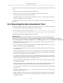
The hifiPipeline task appears in the "Applicable" Folder in the Tasks view after clicking on the Observation Context (MyObs) in the variable view.
Figure 2.1. HIFI pipeline task: default view
Running the hifiPipeline GUI:
The default (or basic) dialogue allows you to re-process an already existing observation context, e.g.
from the Herschel Science Archive, through the pipeline. The default set-up of the pipeline is to reprocess data from level 0 to 2 for all four spectrometers (or as many as were used in the observation).
• The way the data is to be reprocessed is defined in the Input section:
1. If the hifiPipeline task was opened from the "Applicable Tasks" folder then the ObservationContext
selected in the Variables View will automatically be loaded into the Task dialogue, and you will
see its name by the observation context bullet, which will be green. Alternatively, drag the name of
the observation context to be reprocessed from the Variables view to the observation context bullet.
2. Select the spectrometers you wish to process data for by checking the desired instrument(s) and
polarisation(s). Both H and V polarisations of both the Wide Band Spectrometer (WBS) and High
Resolution Spectrometer (HRS) are checked by default.
3. Select which levels to (re-)process from and to via the drop-down menus. By default the pipeline
will process level 0 data up to level 2. Data taken from the Herschel Science Archive (HSA) can
be re-processed from level 0 (option 0) to levels 0.5 (option 0.5), 1 (option 1), or 2 (option 2)
If you try to re-process from a higher Level data than exists in the Observation Context then the
hifiPipelineTask will automatically select the highest existing Level. For example, if you try to reprocess from Level 0.5 to 1 but the ObservationContext only contains a Level 0 product then the
pipeline will automatically run from Level 0 to Level 1.
5
Running the HIFI pipeline
4. You can supply your own algorithm to the pipeline (see Section 2.4). Click on the folder to browse
for the file, or supply the full path in the text box. The ways you might want to modify the pipeline
algorithms are discussed in Section 2.3. See the notes below about customizing pipeline algoriths.
• In the Output section, choose the name of the observation context that will be produced or use the
HIPE default, obs.
• Click on "accept" to run the pipeline. The status ("running" if all is well, error messages if not)
and the progress of the pipeline are given in the Info section at the bottom of the Task dialogue.
You will also see more informative messages about the status of the pipeline written in the console
and terminal.
Saving the output:
There are several methods you can use to save your reprocessed observation.
• Right click on the output ObservationContext obs and select "Send to Local store"
• When you run the pipeline, you can specify which pool the output should be written to. In the
console type,
name="My-pipeline-out"
pool=ProductStorage(LocalStoreFactory.getStore (name))
and drag pool to the palStore bullet in the GUI.
The "Expert" mode of the hifiPipeline is intended for Calibration Scientists and Engineers, and is not
described here.
2.2.2. The hifiPipeline in the command line
Below are some examples of running the hifiPipeline task from the command line, once again it is
assumed that an ObservationContext called Myobs has been loaded into the session.
# Reprocess an ObservationContext up to Level 2 for all spectrometers:
MyNewobs = hifiPipeline(obs=Myobs)
#
# Reprocess Myobs from Level 0.5 to Level 1, for all spectrometers:
MyNewobs = hifiPipeline(obs=Myobs, FromLevel=0.5, UpToLevel=1)
#
# Now reprocess MyNewobs (which now contains data only up to Level 1) but only for
the WBS.
# WBS-H and WBS-V are the horizontal and vertical polarizations, respectively:
MyEvenNewerobs = hifiPipeline(obs=MyNewobs, apids=['WBS-H', 'WBS-V'])
#
# Reprocess Myobs from Level 0 to Level 0.5 for only horizontal polarization data:
MyNewobs = hifiPipeline(obs=Myobs, apids=['WBS-H','WBS-V'], FromLevel=0,
UpToLevel=0.5)
#
# Now include your own algorithm for the Level 1 pipeline, for all spectrometers,
from Level 0 to 1:
MyNewobs = hifiPipeline(obs=Myobs, FromLevel=0, UpToLevel=1,
level1Algo={full_path}mylevel1Algo.py)
#
# Specify the pool to which the pipeline should write output:
name="My-pipeline-out"
pool=ProductStorage(LocalStoreFactory.getStore (name))
MyNewobs = hifiPipeline(obs=Myobs, palStore=pool)
#
# If the pipeline is not behaving as you expect (keeping old values, for example)
try resetting it:
hifiPipeline = hifiPipelineTask()
#
6
Running the HIFI pipeline
• The exact ordering of the arguments does not matter.
• What is an apid? "Application Program IDentifier": it is what the pipeline calls spectrometers.
• Note that to implement your own algorithm, you must load the algorithm script from wherever you
saved it into HIPE and compile it (run it with >>) before you run the pipeline (see Section 2.4).
To save MyNewObs to pool:
storage = ProductStorage()
pool = PoolManager.getPool("MyPool")
storage.register(pool)
storage.save(MyNewObs)
2.3. Running the Pipeline step by step
• Running the pipeline, or one part of the pipeline, step by step allows you to inspect the results of each
step and change the default parameters of the pipeline. If you wish to create your own algorithm,
which must be written in jython, for a part of the pipeline, then this will likely be your first step.
• It is not expected that there will be much need to customise the spectrometer pipelines (up to Level
0.5) and indeed there are only a few steps of the spectrometer pipelines that have some options. It
is more likely that you may wish to play with how off and reference spectra are subtracted in the
Level 1 pipeline, although it is expected that the default settings should work well.
• To step through the pipeline you must work directly on the appropriate level HifiTimeLine (HTP
- the dataset containing all the spectra, including calibration spectra, made during an observation
for a given spectrometer). So the first thing you must do is extract the HTP you want to work on
from your ObservationContext:
• Drag an HTP from the ObservationContext tree in either the Context Viewer or Observation
Viewer into the Variables view, and rename it if you desire by right clicking on the new variable
and selecting "rename".
• In the command line, the formalism to extract an HTP is
htp = obs.refs["level2"].product.refs["HRS-V-USB"].product
"level2" and "HRS-V-USB" should be replaced by the level and backend combination desired.
• When you select an HTP in the Variables view in HIPE you will notice that many tasks with names
like DoWbsDark, mkFreqGrid. These are the names of all of the steps in the HIFI pipeline; mk...
signifies a step where a calibration product is being made, Do... is a step where a calibration is
applied. You can step through the pipeline using these tasks or (more efficiently) use and modify
the scripts that are supplied with the software in the scripts/hifi/Pipeline directory in the
installation directory of HIPE
• For information on the steps of each level of the pipeline (their names, the order to run them in, and
what options you can change) see the HIFI Pipeline Specification document, see ????.
2.4. How to customise pipeline algorithms
1. The pipeline algorithm scripts can be found in:
• WBS. $BuildDir/scripts/hifi/pipeline/wbs/WbsPipelineAlgo.py
• HRS. $BuildDir/scripts/hifi/pipeline/hrs/HrsPipelineAlgo.py
• Level 1.
$BuildDir/scripts/hifi/pipeline/generic/Level1PipelineAlgo.py
7
Running the HIFI pipeline
• Level 2.
$BuildDir/scripts/hifi/pipeline/generic/Level2PipelineAlgo.py
2. Open the algorithim you wish to customise in the editor, edit it (and save!)
3. Compile your algorithm by running the script with >>
4. Apply the algorithm to the pipeline as described in the sections above.
8
Chapter 3. Flags in HIFI data
Last updated: 11 Feb 2010
3.1. Introduction to flags
Flags (also called masks) are identifiers of specific issues with the data, such as saturated pixels or a
possible spur, that can affect the quality of the final product. Flags are used to identify affected data
and to make a caution during its processing.
A Flag has a defined name and a value, which specifies the nature of the flag. The flags are divided
into two categories, depending on whether they apply to an individual channel (pixel), or to a complete
Dataframe. They are called channel f lags, and column rowflags, respectively.
Note
There are also Quality Flags, which are found in the Quality Product in the ObservationContaxt and are used to provide you with means to make a quick assessment of the quality
of your data, they are discussed in chapter Chapter 4
3.2. Channel flags
Channel (or pixel) flags apply to individual pixels and are added as a column in the HTP. Their names
are also added to the metadata of a dataset during processing and this is used for the history of the
pipeline; it also means that you can tell that, e,g., the WBS pipeline has been applied if you see things
like "isMasked" and "checkZero" in the metadata.
For each pixel there are 32 flags which can be set, currently 8 are defined, and the definition of the
mask bits and values in HIFI data is given here:
Flag Name
Value
Description
Bad pixel
0
If this bit is set, the sample contains a bad pixel
Saturated pixel
1
If this bit is set, the sample was
saturated
Not observed
2
If this bit is set, the sample is
not observed
Not Calibrated
3
If this bit is set, the sample is
not calibrated
In overlap region
4
If this bit is set, the sample is in
the subband overlap region. I.e.
it can be seen better in the adjacent subband.
Glitch detected
5
If this bit is set, the sample is
not observed
Dark pixel
6
If this bit is set, the sample is
used to measure the dark
Spur candidate
7
If this bit is set, the sample is
a candidate to be a spur. It is a
'candidate' since not all things
flagged by the spurfinder are
necessarily spurs
9
Flags in HIFI data
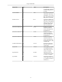
3.3. Column rowflags
Column rowflags (the "rowflag" column in the HIFI spectrum TableDataset) apply to the complete
Dataframes (DF) or rows in a HifiSpectrumDataset (HSD).
For bit n the value is computed according to value=2(n-1). The first 5 bits are about the packets from
which the DataFrame (DF) is reconstructed, and are unlikely to ever occur. Below is a table showing
the current names and values of HIFI rowflags:
Flag Name
Bit
Value
Description
PacketOrder
1
1
Error in the packet order while constructing
the DataFrame
PacketLength
2
2
Error in the packet
length while constructing the DataFrame
TooMuchData
3
4
More data than can be
fit in a DataFrame
FirstPacket
4
8
Error in the start packet
while constructing the
DataFrame
NoBlocks
5
16
No block information
present while constructing the DataFrame
spare
6
32
spare
7
64
UnalignedHK
8
128
HK could not
be aligned with
DataFrames. When the
columns "df_transfer"
and "hk_transfer" in the
TableDataset are different, bit 8 is set
noChopper
9
256
No valid Chopper information. Set when
the flagbit is zero in the
DFs, extracted from the
HK packets if possible
noComChop
10
512
No valid Commanded
Chopper information.
Set when the flagbit is
ero in the DFs, extracted from the HK packets
if possible
noFreqMon
11
1024
No valid Frequency
Monitor information.
Set when the flagbit
is zero in the DFs, extracted from the HK
packets if possible
noLoCodeOffset
12
2048
No valid LO code offset information. Set
when the flagbit is ze-
10
Flags in HIFI data
Flag Name
Bit
Value
Description
ro in the DFs, extracted
from the HK packets if
possible
noLoCodeMain
13
4096
No valid LO code main
information. Set when
the flagbit is zero in the
DFs, extracted from the
HK packets if possible.
BbidCorrection
14
8192
Correction of Bbid, see
SPR 1963. Not relevant
any more. It was during
SOVT testing, but the
onboard software has
been corrected since
MixerCurrentDeviation 15
16384
Difference in mixer
currents exceeds tolerance when applying
DoRefSubtract.
MixerCurrentDeviation 16
32768
Difference in mixer
currents exceeds tolerance when applying
DoOffSubtract.
MixerCurrentDeviation 17
65536
Difference in mixer
currents exceeds tolerance when applying
DoFluxHotCold or MkFluxHotCold.
NoHotColdCalibration 18
131072
Division by the bandpass has not been carried through
SuspectLO
19
262144
LO Frequency is listed
in the Bad Frequency
Table. Data not necessarily is corrupted
SpurDetected
20
524288
Spur detected in the
cold load. Data (partial
or total) is corrupted
IgnoreData
21
1048576
User has the option to
set this flag. Some tools
(e.g. doDeconvolution)
will honor it
11
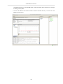
Flags in HIFI data
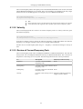
Caption: Example of a HIFI spectrum TableDataset, which contains the "rowflag" column with a value
of 256.
12
Chapter 4. Quality Flags
Last updated: 10 Feb, 2010
Quality Flags are raised during standard processing of HIFI data. Flags should be created from every
processing step of the pipeline, from the initial creation of the HifiTimelineProduct (Level 0), through
to the final product of Level2 processing. If all goes well, the flags will have their default values but
if a certain processing step is unable to perform the action it was designed for the flag will take a
different value. If the pipeline produces a flag other than the default value, this flag is promoted to the
Quality Report. Thus the quality report is by definition a list of things identified as have gone wrong.
A quality report is found from the ObservationContext:
obs.refs["quality"].product
Please note the difference between a quality flag and flagging data. In flagging data you identify that,
for example, a given channel sample is saturated; if those channels are saturated repeatedly during the
observation then the quality flag "SATURATEDNUMBER" wil be raised.
Below is a list of the current available types of quality flags for the HIFI pipeline, for each level. The
format below gives flag name, flag description, and flag default value.
Level O Quality Flags.
Quality Flags
UNALIGNED_HK("unalignedHKdata","Percentage of Dataframes which have unaligned HK",
0.0)
NOCHOPPER("noChopperHKdata","Percentage of DFs having no chopper information", 0.0)
NOCOMCHOP( "noCommandedChopperHKdata","Percentage of DFs having no commanded
chopper information", 0.0)
NOFREQMON( "noFrequencyMonitorHKdata", "Percentage of DFs having no frequency monitor
information", 0.0)
NOLCOFFS( "noLoCodeOffsetHKdata","Percentage of DFs having no LO Code offset information", 0.0)
NOLCMAIN( "noLoCodeMainHKdata","Percentage of DFs having no LO Code main information", 0.0)
BBID_CORRECTION( "bbidCorrection","Percentage of Bbids corrected according to commanded
Bbids", 0.0)
DATAFRAMES_OUTOFORDER( "dataframesOutOfOrder","Unordered or duplicate Dataframes
found", false)
MISSING_DATA( "missingData","Less data found than expected", false)
SURPLUS_DATA( "surplusData","More data found than expected", false)
Quality Flags with
specified thresholds
Range
Consequences for sci- Action required
ence data
FPU_MIXER_CURRENT("mixerCurrent","FPU
[I_leak+5µA,
maybe a degraded
Check: Mixer current is 2xnom_value], for SIS baseline
Out Of Limit", false)
[30µA, 60µA], for HEB maybe a degraded
baseline quality
13
Quality Flags
Quality Flags with
specified thresholds
Range
Consequences for sci- Action required
ence data
FPU_MIXER_CURRENT_VARIANCE("mixerCurrentVariance","FPU
maybe a degraded
Check: Mixer current
baseline quality
variance is Out Of Limit", false)
FPU_MIXER_VOLTAGE("mixerVoltage","FPU
[nom_value-100µV,
maybe a serious probCheck: Mixer Voltage nom_value+100µV]
lem
is Out Of Limit", false)
Inform engineering
team
FPU_MIXER_MAGNET_CURRENT("mixerMagnetCurrent","FPU
[nom_valuex0.96,
baseline could be unCheck: Mixer Magnet nom_valuex1.04]
stable
Current is Out Of Limit", false )
FPU_MIXER_MAGNET_RESISTANCE("magnetResistance","FPU
[nom_valuex0.8,
serious problem
Check: Mixer Magnet nom_valuex1.2]
Resistance is Out Of
Limit", false )
Inform engineering
team
FPU_CHOPPER("fpuChopper","FPU
[nom_offset-0.05 V,
Check: chopper meanom_offset+0.05 V]
sured values differ
from the commanded",
false )
Check other pointing
out of limit flags
potential pointing or
readout problems
FPU_DIPLEXER_RESISTANCE("diplexerResistance","FPU
[nom_valuex0.8,
serious problem
Check: Diplexer Resis- nominal_valuex1.2]
tance is Out Of Limit",
false )
Inform engineering
team
FPU_LNA("lna","FPU [-1.5 V, +0.5 V]
Check: IF Amplifier
values are Out Of Limit", false )
IF power level ok? --> Inform engineering
maybe unstable base- team
line. Level dropped?-->
transistor faulty
FPU_HOT_LOAD("hotLoad","FPU
[90,110 K]
Check: Hot load temperature is Out Of Limit", false )
serious problem with
the heater or with the
readout
Inform engineering
team
SFPU_COLD_LOAD("coldLoad","FPU
[4, 20 K]
Check: Cold load temperature is Out Of Limit", false )
serious problem
Inform engineering
team
FPU_LEVEL_TEMP("l0Temp","FPU
[1.5, 2.5 K]
Check: Level 0 Temperature is Out Of Limit", false )
serious problem with
the thermal environment or with the readout
Inform engineering
team
Level 0.5 Quality Flags: WBS.
Quality Flags
COMBFLAG(QWbsFreq.VALIDATE,"Flag for all COMB of the observation",false)
ZEROFLAG(QWbsZero.VALIDATE , "Flag for all Zero of the observation",false)
SPIKENUMBER(QWbsSpikes.NUMBER, "Maximum number of spikes detected in a Comb", 0)
SATURATEDNUMBER("pixelSaturated","Maximum number of saturated pixel detected in a single spectrum",0l)
SDARKFLAG("darkFlag","Spectrum contains saturated dark ",false)
14
Quality Flags
Quality Flags
BADPIXELS("badPixels","Number of channels marked as BAD due repeated saturations",0l)
Level 0.5 Quality Flags: HRS.
Quality Flags
NOQDC("noQDC", "No Quantization Distortion Correction could be processed.",false)
FASTQDC("fastQDC", "Fast Quantization Distortion Correction processed. Not optimal.",false)
NOPOWCOR("noPowerCorrection","No Power Correction could be processed.",false)
Level 1.0 Quality Flags.
Check data structure.
Quality Flags
OBSERVINGMODE("observingMode","Observing mode not recognized - consult the pipeline
configuration xml file.", false)
UNKNOWNBBTYPE("unknownBbType","Bbtype not known.", false)
Check freq grid.
Quality Flags
FREQUENCYDRIFT("maxFreqDrift", "Unacceptable maximum drift in the frequency grid detected.", false)
FREQUENCYCHECKS("noFreqChecks", "Frequency checks and/or frequency grouping failed.",
false)
Check phases.
Quality Flags
CHOPPERPATTERN("chopperPattern", "Pattern observed for the Chopper not as expected in all
datasets.", false)
CHOPPERVALUES("chopperValues", "Number of distinct Chopper values not as expected in all
datasets.", false)
LOFPATTERN("lofPattern", "Pattern observed for the LoFrequency not as expected in all
datasets.", false)
LOFVALUES("lofValues", "Number of distinct LOF values not as expected in all datasets.", false)
BUFFERPATTERN("bufferPattern", "Pattern observed for the buffer not as expected in all
datasets.", false)
BUFFERVALUES("bufferValues", "Number of distinct buffer values not as expected in all
datasets.", false)
PHASECHECKS("noPhaseChecks", "Not all phase checks could not be carried through or completed.", false)
Hot/cold-calibration.
Quality Flags
HOTCOLDDATA("hotcoldData","Data measured from hot and cold loads not sufficient for hot/
cold calibration.", false)
TSYSFLAG("tsysFlag","Hot/cold calibration not successful.", false)
15
Quality Flags
Quality Flags
INTENSITYCALIBRATION("intensityCalibration", "Intensity calibration not or not for all spectra carried through.", false)
Channel weights.
Quality Flags
CHANNELWEIGHTSFLAG("channelWeights","Problem occurred while computing channel-dependent weights. No weights added.", false)
Reference subtraction.
Quality Flags
REFSUBTRACTIONFLAG("refSubtraction", "Reference subtraction not processed - maybe identification of phases not successful.", false)
Off smooth.
Quality Flags
NOOFFBASELINE("noBaseline", "No off baseline could be calculated.", false)
Off subtraction.
Quality Flags
ONOFFSEQUENCE("onoffSequence","ON/OFF datasets not in expected sequence (...-ON-OFFON-OFF-... or ...-ON-OFF-OFF-ON-ON-....", false)
ONOFFPAIRSIZE("onoffLength", "Some ON/OFF dataset pairs found with unequal number of
rows.", false)
ONOFFPROCESSING("onoffProcessing", "More ON- than OFF-datasets found in the data - not
all ON-datasets could be processed with OFF-dataset(s).", false)
OFFBASELINESUBTRACTION("offBaselineSubtraction", "No off baseline subtraction carried
through since no off baseline data available.", false)
DATALOSSINAVERAGE("average", "Some data has been lost while computing the average over
many datasets.", false)
16
Chapter 5. Viewing Spectra
Last updated: 19 Dec, 2009
5.1. Introduction
HIFI spectra can be visualised in several ways, at various levels of sophistication and user-friendliness.
Here the PlotXY and SpectrumExplorer packages are described.
5.2. Basic Spectrum Viewing: the PlotXY
Package
PlotXY() is the basic package to plot arrays of data points in the HCSS, and it can be used to plot
HIFI spectra as well. It has a lot of options, making the plots highly configurable. Here is an example
of plotting a HIFI spectrum:
• Get the frequency and flux data to be plotted from the spectrumdataset 'sd':
freq=sd.getWave().get(0)
flux=sd.getFlux().get(0)
• The simplest possible plot:
out=PlotXY(freq, flux)
• When plotting multiple spectrum datasets, say 'sd1' and 'sd2' in one figure:
#get the wavelengths and fluxes to be plotted
freq1=sd1.getWave().get(0)
flux1=sd1.getFlux().get(0)
freq2=sd2.getWave().get(0)
flux2=sd2.getFlux().get(0)
#create the plot variable
p=PlotXY()
#create the plots in batch mode
p.batch=1
#define the layer variable
ll=[]
#remove any non-numbers (NaN's, Infinites etc.)
valid=flux1.where(IS_FINITE)
#create layer for first plot
l=LayerXY(freq1[valid],flux1[valid])
17
Viewing Spectra
#append to layer variable
ll.append(l)
#repeat the above for the 2nd plot to be overlaid
valid=flux2.where(IS_FINITE)
l=LayerXY(freq2[valid],flux2[valid])
ll.append(l)
#define the plot layers that have just been created
p.layers=ll
#get out of batch mode. This actually creates the plot
p.batch=0
• And this is how some common features of the plot are modified.
p.setYrange([0, 1.5])
p.setTitleText("This is an example plot")
5.3. Viewing with SpectrumPlot
It is also possible to display spectra without taking apart the data format as is described in the previous
section. All Herschel spectra types can be displayed with the SpectrumPlot package.
If spectrum is a Herschel Spectral type (Spectrum1d, Spectrum2d) then:
splot=SpectrumPlot(spectrum, useFrame=1)
will simply display the spectrum along with some standard header information. The useFrame=1
allows for the possiblility of creating a plot without actually viewing it at first, but as the last step. The
SpectrumPlot module is build on PlotXY, and so many of the features you would use in PlotXY you
can also use for SpectrumPlot. Below are a few examples:
from herschel.ia.toolbox.spectrum.gui import SpectrumPlot
from herschel.ia.gui.plot.renderer.StyleEngine.ChartType import HISTOGRAM,LINECHART
#
#
Creating the plot
sp=SpectrumPlot(spectrum,useFrame=1)
#
#
adding a second spectrum to the plot
sp.add(spectrum2)
#
#Start
fresh again
p = SpectrumPlot(spectrum, useFrame=1)
#
#get
graphs
g0 = p.getGraphs()[0]
g2 = p.getGraphs()[2]
#
#display as line graph or histogram
g0.layer.style.chartType = HISTOGRAM
18
Viewing Spectra
g2.layer.style.chartType
= LINECHART
#
#add
annotations
g0.layer.addAnnotation(Annotation(4000,1,"My
annotation"))
g0.layer.addAnnotation(Annotation(5000,0.98,"My
annotation"))
#
#select
a range of data
g0.layer.xaxis.addMarker(AxisMarker(4200,4400))
g2.layer.xaxis.addMarker(AxisMarker(6000,6500))
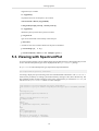
These last lines will produce the following plot:
Figure 5.1.
5.4. The SpectrumExplorer Package
5.4.1. Starting the SpectrumExplorer
The SpectrumExplorer package allows one to visualize HIFI, PACS, and SPIRE SpectrumDatasets in
a userfriendly, interactive way. To activate it, click on a SpectrumDataset or Product in the Variables
window or Observation Viewer with the right mouse button and select 'Open With' and 'Spectrum
Explorer'. If this is the default, it suffices to double-click on the variable.
19
Viewing Spectra
Initially an empty plot is displayed in the top part of the window that is opened and a selection panel
is displayed in the bottom part.
The look of the selection panel depends on the SpectrumDataset type. A typical example is displayed
in the following picture. When the added SpectrumDataset is a SpectralCube, a cube visualizer is
displayed instead with which spectra can be selected.
When a Product is selected for display, the bottom part will show a 'loading datasets...' message as
long as the Product is being processed. Each SpectrumDataset found in the Product is added to the
selection panel.
The location of the divisor between both panels can be changed through drag drop interaction. Clicking
on one of the little black arrows displayed on the left edge of this divisor extents a single panel to
its full size.
5.4.2. Selecting Spectra
The attribute columns in the selection panel can be used to find spectra that one wishes to plot. A
single click on a header of such column sorts the rows according to that column's entries. Clicking it
again inverts the sort order. A double click removes the sort and therefore brings the ordering back
to its initial state.
With drag and drop, the columns themselves can be reordered. A right click on one the headers shows a
dialogue box with a selection list of all column headers. With this list the columns can also be reordered
or even hidden from view. Hold the shift button to hide/display a whole range of columns at once.
Furthermore, specific spectra can be selected by applying a filter on the attribute columns. Open the
filter panel by selecting Dialogs -> Filter from the right-mouse click menu or by clicking on the filter
icon in the button toolbar at the top of the HIPE screen. Specify the attribute name (from one of
the column headers) and enter the filter values, that can be ranges, circular ranges or exact values.
20
Viewing Spectra
The filters are combined by applying the 'AND' operator. Clicking on the green circle next to a filter
temporarily disables that filter. Clicking on the red cross removes it from the panel.
5.4.3. Displaying Spectra
In the general selection panel at the bottom, each row depicts an individual spectrum. The numbers in
the first column show the index of the spectrum within the SpectrumDataset. If SpectrumExplorer was
opened on a Product, the index is preceded by the index of the SpectrumDataset within the Product.
For example, 2.3 denotes the fourth spectrum within the third SpectrumDataset within the Product
(given that both indices start with 0).
Clicking the button in the first column displays all segments in that spectrum. A double-click removes
them from the plot. The same accounts for the top row of buttons: clicking displays a single segment
for all spectra, while double-clicking removes them from the plot. The 'ALL' button in the top left
corner of the selection panel displays all segments of all spectra. Finally, individual segments can be
displayed by the clicking the approprate box. The colour of the button is changed to the colour of
the spectrum displayed in the plot. In case a Product is displayed with SpectrumDatasets containing
different numbers of segments, the invalid segments are disabled and displayed with a grey 'x'. An
example is shown in the figure above.
5.4.4. Button Bar
At the top of the HIPE screen, the SpectrumExplorer buttons following the 'New...' and 'Open File...'
buttons have the following meaning:
• button 1: save the plot as a PNG, PDF, EPS or JPEG file
• button 2: send the plot to the printer
• button 3: zoom mode. This is the default mode when SpectrumExplorer is started. Change the horizontal and vertical plot ranges by drawing a rectangular box using the left mouse button. Control-left
mouse button will un-zoom the plot (or use the Autorange option under the right mouse button).
• button 4: select spectra. A clicked spectrum will be displayed with a bold line. Any operation, such
as the Tasks under the right mouse button, will then only apply to this particular spectrum. Also
21
Viewing Spectra
the selected spectrum can be dragged to a new panel (note that dragging to the left and top of the
original panel is not possible). The spectrum can also be dragged to the Variables window where
it will be stored as a new variable.
• button 5: pan mode. Pan through the spectrum by clicking the left mouse button and moving the
mouse. If one only wants to pan along the x or y axes, click on the axis with the left mouse button
and then move the mouse (or use the mouse wheel).
• button 6: select ranges. Click and drag to select ranges in a plot (the middle mouse button can be
used anytime for this as well). This will create a vertical grey bar. Then in the spectrum selection
mode (button 4), only this will be saved as a new variable.
• button 7: select points. Click and/or drag with the left mouse button to select one or more spectral
points. These points can later be flagged or removed.
• button 8: (de-) activate preview mode. In preview mode a quick preview is displayed of all rows
selected in the selection panel.
• button 9: display/hide grid in the active sub plot
• button 10: display/hide the plot legend
• button 11: switch between line and histogram mode
• button 12: display flagged channels
• button 13: show/hide the plot title
• button 14: open filter panel
• button 15: show metadata of the displayed SpectrumDataset
• button 16: open a raster panel showing all plots in the selection panel
• button 17: open the properties panel in the top-right part of the SpectrumExplorer to view and
modify any plot parameter. The panel can also be opened using the 'Properties...' option under the
right-click popup menu. If a paricular element in the context contains no changeable properties, the
plot properties are displayed.
5.4.5. Plot Interactions
The Spectrum Explorer provides context-dependent plot interactions. The behaviour of mouse interaction depends on the location of the mouse cursor. The actual context is displayed in the left bottom
corner of the plot panel. Next to the context you'll find the location of the mouse cursor in plot coordinates. The following table provides the some contexts and the mouse interaction behaviour.
Context
Click
Subplot
Set as 'active'
Ctrl-click
Axis
Spectrum
Select spectrum
Extend selection
Select point
Drag
Scroll
Zoom/Select/Pan
Zoom
Pan
Zoom
Move spectrum to
another subplot
Extract spectrum
to a new variable
Use spectrum as
task input parameter
Selection
Same as above
22
Viewing Spectra
Context
Click
Ctrl-click
Marker edge
Drag
Scroll
Resize marker
A right click on a plot shows a popup menu with global and context specific options. Right clicking
below or besides a plot gives the option to add another subplot in that place. The new subplot becomes
'active'. New selected spectra are displayed in the active subplot. To activate another subplot, right
click on that subplot and check the radio button named 'active'.
5.4.6. Raster Panel
When SpectrumExplorer is used in raster mode (selected using the Raster button at the top button bar),
a single spectrum is plotted plot for each row in the selection panel. This selection can be altered by
making use of the filter panel. When all spectra contain pointing information, the plots are laid out on
a latitude/longitude plane. Otherwise the plots are displayed in a rectangular grid.
The wave and flux ranges above the plot can be altered by textual input or by scrolling on top of the
text field. After doing this, the slide bars below the ranges can be used to slide the sub range through
the plots.
Use the scroll wheel on top of the plot to zoom. A single click on a plot opens the spectrum in the
plot view of the SpectrumExplorer.
5.4.7. Preferences
Default SpectrumExplorer settings can be modified using the Edit-->Preferences button at the very
top of the HIPE screen. The following options are available:
• Initial tool: specifies whether the Spectrum Explorer should start in zoom or select mode.
• ChartType: display plot in line style or histogram
• Display grid: on or off
• Display legend: on or off
• Start in preview mode: on or off
For a specific SpectrumDataset type, title/subtitle and legend element can be specified. Metadata fields
and attribute fields can be filled in automatically by specifying the fields name between angular brackets. Optionally with a printf-style format suffix. For example
longitude%.2f"
in the legend element field displays the value of the longitude attribute for each spectrum in the legend
23
Chapter 6. Changing to LSB/USB and
Velocity
6.1. Changing HIFI Frequency Scales
In practice there at two methods of altering the HIFI frequency scales: using the Spectrum Explorer
GUI or from the command line. These two approaches differ in one fundamental way. The command
line tasks will actually change the data, by resetting the frequency to upper/lower sideband representation or velocity. The GUI only changes what is seen in the SpectrumExplorer, the data themselves
are not changed.
There are four fundamental ways of representing the frequency scale for HIFI: the intermediate frequency (default), the upper sideband frequency, the lower sideband frequency, or by velocity.
One final note, currently the HIFI pipeline is providing the "final" spectra represented in both USB
and LSB. The level 2 product names are tagged LSB or USB it is still possible from these spectra to
transform back to IF or the other sideband.
6.1.1. Changing Spectral Views
The SpectrumExplorer provides internal means of viewing spectra. These views are only for display
purposes and do not change the data.
6.1.1.1. LSB/USB
Assuming you have activated a spectrum in a SpectrumExplorer window. To move between a spectrum
seen in the Intermediate Frequency, USB or LSB, right mouse click on the frequency access (not the
title of the access, but the axis itself). A pull down menu for the access will appear.
6.1.1.2. Velocity
6.1.2. Change Spectral Views from the command line
6.1.2.1. LSB/USB
The task to convert the actual frequency scale in a HifiTimelineProduct or HifiSpectrumDataset is
called ConvertFrequencyTask. Assuming spectrum is the variable name for a HifiSpectrumDataset
with the frequency scale of the data in expressed as IF frequencies.
cft=ConvertFrequencyTask()
cft(sds=spectrum,to="lsbfrequency")
Of course, it is also possible to convert to the upper sideband. for this the keyword is "usbfrequency".
cft(sds=spectrum, to='usbfrequency')
To convert back to the IF, use:
cft(sds=spectrum, to='frequency')
24
Changing to LSB/USB and Velocity
The ConvertFrequencyTask works equally well on the HifiTimelineProduct itself. In this case all the
internal HifiSpectrumDatasets are converted. This is not something you should do in the early stages
(before level 0.5) of the HIFI pipeline. For example on a level 1 HifiTimelineProduct:
cft=ConvertFrequencyTask()
cft(htp=hifitimelineproduct, to='frequency')
Note
Direct application of the ConvertFrequencyTask changes the data listed in the spectrum.
Conversion back to the original IF scale is possible, just use the to='frequency' option.
6.1.2.2. Velocity
The ConvertFreqencyTask also works to convert the frequency scale to a velocity scale once given
the reference frequency.
cft=ConvertFrequencyTask()
cft(sds=spectrum,to='velocity',reference=576.268,inupper=False)
In the above example, I had to specify the reference frequency in GHz and whether this reference
frequency is for the upper (inupper=True) or lower (inupper=False) sideband.
Another call to ConvertFrequencyTask using "to = 'frequency'" will undo the change to velocity as
well.
6.1.2.3. Review of ConvertFrequencyTask
The ConvertFrequencyTask works on HifiSpectrumDatasets or HifiTimelineProducts. The task uses
the keywords "sds" for HifiSpectrumDataset and "htp" for HifiTimelineProducts. The conversion of
frequencies is done using the "to" keyword. The following table shows the various possibilities:
to=
Description
Other keywords necessary
frequency
Converts to the Intermediate
Frequency scale.
None
usbfrequency
Converts to the Upper side band None
Frequency scale.
lsbfrequency
Converts to the lower side band None
Frequency scale.
velocity
Converts to the velocity scale in reference=reference frequency,
km/s
inupper=(True or False)
25
Chapter 7. The Spectral Toolbox
When a spectrum is active (has just been created, or has been selected in the Variables View), HIPE
automatically becomes the Spectrum Toolbox. Your spectrum can be viewed with SpectrumExplorer and this can serve as your launching point for spectral analysis. By right clicking on a spectrum
in SpectrumExplorer and selecting the "Tasks" sub-menu you can access the tasks in the Spectrum
Arithmetics Toolbox and to the Spectrum Fitter Toolbox. The tasks in these Toolboxes are also found
under "Applicable Tasks".
These are general tools available to all Herschel instruments and are described in Chapter 5 of the
Data Analysis Guide.
26
Chapter 8. HIFI Standing Wave
Removal Tool
Last updated: 3 March, 2010
8.1. Introduction to FitHifiFringe
FitHifiFringe is a tool to remove standing waves from level 1 and level 2 HIFI spectra. It makes use of
the general sine wave fitting task FitFringe, but has been adapted to read HIFI data and provide input
and defaults applicable to HIFI spectra. For details on the sine wave fitting method, please consult
the FitFringe manual, ???? .
FitHifiFringe is being tested on PV data. It can be applied to all bands, with the caveat that the standing
waves in HEB bands 6 and 7 are not sine waves, and hence can only be fitted in an approximate way
by fitting a combination of many sine waves.
The GUI and input parameter names of FitHifiFringe are different in HIPE versions 2 and 3. The latter
is more userfriendly, although there is no difference in the functionality.
8.2. Running FitHifiFringe
FitHifiFringe is automatically registered to an ObservationContext (i.e. when clicking on an ObsContext in the Variable window of HIPE, FitHifiFringe shows up as an applicable task). However, the user
can also process a HifiTimelineProduct or a SpectrumDataset instead, by opening the GUI under 'All
Tasks' and then dragging the variable to the appropriate bullet. Alternatively run it on the command
line as follows:
fhf = FitHifiFringe()
fhf(obs1=obs_in,nfringes=2,typical_period=150.,
USB')
product='WBS-H-
obs_out=fhf.result_obs
or for HifiTimelineProducts:
fhf = FitHifiFringe()
fhf(htp1=htp_in,nfringes=2,typical_period=150.)
htp_out=fhf.result_htp
or for SpectrumDatasets:
fhf = FitHifiFringe()
fhf(sds1=sds_in,nfringes=2,typical_period=150.)
sds_out=fhf.result_sds
For HifiTimelineProducts and SpectrumDatasets, the output is identical to the input, but with the fitted
sine waves subtracted from the flux columns. For ObservationContexts, the input has the sine waves
subtracted as well (this is a HIPE limitation, which may be changed in the near future).
Besides obs1, htp1, and sds1, the following input parameters are allowed:
27
HIFI Standing Wave Removal Tool
• product: if the input is an ObservationContext, indicate which level 2 product needs to be processed.
Options are: 'WBS-H-USB', 'WBS-H-LSB' 'WBS-V-USB', 'WBS-V-LSB' 'HRS-H-USB', 'HRS-HLSB' 'HRS-V-USB', 'HRS-V-LSB'
• nfringes: number of sine waves to be fitted [DEFAULT: 1]
• start_period: shortest-period standing wave (in MHz) to search for [DEFAULT: start_period=20]
• end_period: longest-period standing wave (in MHz) to search for [DEFAULT: end_period=3000]
• typical_period: typical standing wave period (in MHz) in the data. This is used for the baseline
determination. Features with much longer periods are considered baseline structure and will not be
removed with sine waves. [DEFAULT: typical_period=150.]
• plot=False: only show plot of end-result for each scan [DEFAULT: 2 plots per scan: (1) period
versus Chi^2 (2) the before/after plot and the subtracted sine wave and the line mask]
• averscan=True: determine standing waves on average of all scans, and then subtract this from each
scan [DEFAULT: process each scan separately]
• doglue=False, Determine SW on individual sub-band spectrum. This is desired for HRS, but often
not for WBS, as long period SW can only be determined on the combined spectrum. [DEFAULT:
doglue=True]
• usermask=..., mask frequency ranges in addition to the automatically determined mask. Example:
usermask=[(537.0,538.0), (539,539.5)] masks the ranges 537-538 GHz and 539-539.5 GHz [DEFAULT: only use automatically determined mask]
28
Chapter 9. Sideband Deconvolution
Last updated: 1 March, 2010
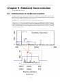
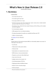
9.1. Introduction to doDeconvolution
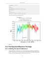
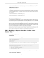
The deconvolution tool is the post-Level 2 processor to separate the "folded" double sideband (DSB)
data inherently produced by the heterodyne process into a single sideband (SSB) result. See the figure
below. Fluxes (F_DSB) in the DSB spectrum are given by:
F_DSB(nu_IF) = g_u*F_sky(nu_LO+nu_IF) + g_l*F_sky(nu_LO-nu_IF)
where nu_LO+/-nu_IF are sky frequencies, and g_l and g_u are sideband gain (imbalance) factors,
typically close to 1. The deconvolution is used to reduce WBS Spectral Surveys, which are collections
of observations taken at many LO settings so as to constrain the solution. The algorithm finds a SSB
solution that best models the observed DSB observations through iterative chi-square minimization
(Comito and Schilke 2002).
29
Sideband Deconvolution
The deconvolution tool is run AFTER the level 2 pipeline. The level 2 pipeline performs the following
tasks:
• splits the data into upper and lower sideband representations
• applies a gain correction specific to the LO frequency and sideband of the spectra
• corrects frequencies for spacecraft radial velocities
• resamples the spectra onto a fixed grid. For WBS this is done at 0.5 MHz spacing, with the first
frequency snapped to the nearest 0.5 MHz
Any HIFI observation context will contain Level 2 products if run through the standard product
generation.
9.2. Running the Deconvolution Tool
Assuming the observation context is named "MyObsContext", the user can run the deconvolution task
on the command line with the default parameters by simply invoking:
result=doDeconvolution(obs=MyObsContext)
The full range of parameters and their defaults are as follows:
decon_result
=
doDeconvolution(polarization=0,bin_size=5.0E-4,max_iterations=200,
tolerance=0.0010,gain=0,channel_weighting=False,ignore_mask=524288,plot_dsb=0,
use_entropy=False,lambda1_channels=0.0,lambda2_gains=0.0,cont_offset=0.0,expert=
• polarization: Observations contexts store H and V polarisations. You can specify which to deconvolve with this option. 0=H, 1=V
• bin_size: Tells deconvolution the sampling interval of the single sideband solution. A value of 0.5
MHz is recommended to match the WBS sampling.
• max_iterations: Tells doDeconvolution to stop after a specified number of interations if it has not
converged by then
• tolerance: Specifies the tolerance of the solution. When the rms of the residual of the fit changes
fractionally by less than tolerance, the algorithm stops iterating. A value of 0.001 is best. Below
this value, the algorithm may produce poor baselines.
• gain: Toggles gain optimisation on and off. If on, doDeconvolution will run twice, first with gain
factors set to 1.0 for stability, and then a second time, starting with the SSB solution of the first run,
but this time allowing the gain values to be optimized as well.
• channel_weighting: Toggles whether or not the deconvolution uses the weight values in the data,
to weight less noisy data.
• ignore_mask: Looks for a row mask identifying spurs so strong they corrupt the entire spectrm, and
will ignore that spectrum during deconvolution. The defaults are still being determined.
• plot_dsb: Toggles visualisation on and off. When on, the SSB output solution against the DSB input
can be viewed.
• use_entropy: The user can turn "On" or "Off" terms which incorporate the maximum entropy
method in the deconvolution.
• lamdba1_channels: Used in maximum entropy method. The relative importance of maximizing the
SSB channel entropy of the solution, along with matching the observed spectra is controlled by this
weighting coefficient.
30
Sideband Deconvolution
• lambda2_gains: Used in maximum entropy method. The relative importance of maximizing the gain
entropy of the solution, along with matching the observed spectra is controlled by this weighting
coefficient.
• cont_offset: Used in maximum entropy method. The user can insert a "continuum offset" value to
insure that no negative fluxes enter and disrupt the entropy calculation. The offset is subtracted after
the solution is reached.
• expert: Toggle on an off expert use of the tool, which allows viewing of interim products. These
are a snap-shot of the solution as a function of iteration, and include goodness of fit measurements
such as Chi-squared. Note this is memory intensive, and only available in 3.0.
Maximum Extropy:
The maximum entry option is "turned on" as a "stop-gap" measure to help a bad situation
with the input data. The bad situation can include:
1. Insufficient redundancy, say a redundancy of less than R=4;
2. Too few lines (since line strengths guide the deconvolution);
3. Poor, or excessively noisy data;
4. Also, if the solution of the nominal deconvolution contains periodic noise patterns, or
the solved gains deviate widely from 1.0.
The inclusion of the maximum entropy method adds a term to to the quantity being minimized. Without this term, the quantity being minimized is the Chi-square difference between observed double sideband (DBS) spectra and the modelled DBS spectra. The minimization is accomplished by altering the SSB model spectrum from which the DSB model
spectra are derived. But, when the input data are of poor quality, sparse sampling, or contain few lines, repetitive noise structures may appear in the solution and/or the fitted gain
values may begin to diverge and become non-physical. Since the entropy of these artifacts
is low, we compute the inverse of the solution entropy and add it to the Chi-square value at
each iteration. In this way the deconvolution must still match the observations but has the
additional task of keeping the entropy of its solution high, yielding a non-highly patterned
result. Turning on the entropy terms helps the deconvolution "behave."
The two lamda factors are the two relative weights of the entropy terms for the channel
solution (SSB spectrum) and the gain values. To use the maximum entropy lambda terms,
set the weight low, e.g. channel weight to 10^-5 and gain weight to 0. Slowly increase
either of these weights (10^-4, 10^-3,... and look for an improvement. The weights should
not exceed 10^-1.
The Deconvolution Tool can also be run from a GUI by clicking on the the obs context in the "Variables" window, then double clicking 'doDeconvolution' in the "Task" list.
Like other GUIs in the system, once the 'Accept' button is hit, the command line version is written in
the console window so users know exactly how the task was called. This output can be cut and paste
into user scripts for repeatability.
9.3. Viewing Deconvolution Results
• The output product result can be viewed with the product viewer.
• The single sideband result (ssb) is a dataset that can be viewed with the SpectrumExplorer. On the
command line, it can be extracted from the product as follows: ssb=decon_result["ssb"]
This contains the deconvolved spectrum, and is the primary output of the tool.
• The dataset "gain" can be viewed with dataset inspector. On the command line, it can be extracted
from the product with: gains=decon_result["gain"] The deconvolution tool can estimate
31
Sideband Deconvolution
the sideband gains due to the redundant nature of the data taking. These estimates are stored per
LO tuning in this product.
• The meta data added to ssb includes number of iterations and the tolerance, as can be seen in the
HIPE screenshot below.
32
Chapter 10. How to make a spectral
cube
Last updated: 1 March, 2010
10.1. Introduction to doGridding
Spectral cubes from OTF mapping observations are produced as part of the SPG pipeline and are a level
2 product. However, re-processing of spectral cubes from a Level 2 product is likely desirable; this is
done using the doGridding Task after calibrations of baseline, sideband gain, and antenna temperature.
It is also important that the spectra have been resampled to a linear frequency axis (doFreqGrid in
the Level-2 pipeline).
The default operation of the task is to select the science datasets from an HTP and create a cube for each
given spectrometer subband. Each slice of the cube is produced by computing a two dimensional grid
covering the area of the sky observed in a mapping mode. For each pixel in the grid, the task computes a
normalized Gaussian convolution of those spectra (equally weighted) falling in the convolution kernel
around that pixel. After running the task you will have an array of cubes, one for each subband and,
in 3.0, a "cubesContext" variable that allows you to easily browse the cubes without need to extract
them from the cube array.
The SimpleCube product can be viewed and analyzed in the SpectrumExplorer, see ????, and with the
CubeSpectrumAnalysisToolbox, see ????.
10.2. Using the GUI to make a Spectral Cube
The doGridding Task can be found in the "Applicable" folder of the Tasks view when an HTP is
selected in the variable view; double-click on it to open the dialogue in the Editor View. You can also
find the task under the Task View in 'By Category' -> 'HIFI'.
As a part of the automated (SPG) pipeline, doGridding handles ObservationContexts but if you are
making a cube yourself then you should use a Level-2 HifiTimelineProduct (HTP). The reason for this
is that doGridding assumes that the spectra have a linear frequency axis, and this may not be the case
for Level-0.5 or Level-1 HTP, where there can still be overlap of subbands. Resampling to a linear
frequency axis is carried out in the doFreqGrid step of the Level-2 pipeline.
Using the GUI you can pass an HTP to the task. You can also specify the subbands for which to create
cubes (useful if you know a line falls only in one subband), the beam size, the weights to be used, the
type of convolution filter, and the parameters of the filter.
By hovering the mouse over the parameter names in the GUI, you can find more information and some
tips on usage. There are two drop-down menus in the GUI, one to select the type of weighting - either
all spectra equally weighted, or you can read the weights column from the dataset, which will carry
forward any weightings you have already applied to the data - and one to select either a Gaussian
or a box filter for the convolution. For all the other parameters, you must specify a variable in the
command line and drag that variable to the appropriate bullet to modify the defaults of the task. Here
are some examples.
• subbands: by default, cubes are created for all subbands in the HTP. To specify, for example, subbands 2 and 3 create the variable subbands:
subbands=Int1d([2, 3])
and drag it to the subbands bullet.
33
How to make a spectral cube
• beam: the default half power beam width (beam size) is calculated to be appropriate to the frequency
at which the observation is carried out, but you may wish to simulate a different beam size.
beam=Double1d([40.0])
Drag this to the beam bullet.
• xFilterParams, yFilterParams: the appropriate values for these depend on the filter being used (box
filter or the default Gaussian), see the next section for more notes. Here an example appropriate
for a box filter.
xFilterParameters = Double1d([0.5])
yFilterParameters = Double1d([1.5])
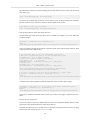
Figure 10.1. The doGridding task GUI form
As with all GUI forms in HIPE, clicking "accept" will start running the task. The outputs you will be
most interested in are the array containing all the cubes created (default name cubes), and the map
context, that allows you to easily browse and view the cubes (default name cubesContext. You
can view these cubes with the SpectrumExplorer and the CubeSpectrumAnalysisToolbox.
There are also other output produced. xPoints and yPoints give the offsets (measured in radians with
respect to the projection centre). The convolutionTable notes which spectra have contributed to each
pixel, but is only generated when the detail tab in the expert GUI is checked.
Clicking on the expert button will toggle to a version of the GUI designed for those who want to really
redesign their cubes. There are many more options available, and they can be passed to the GUI in the
same way. They are discussed in the context of the command line in the next section.
10.3. Making a Spectral Cube via the command line
Some examples of usage are below:
• Data selection:
Make cubes for all the subbands, then display the first one:
cubes = doGridding(htp=htp)
cubes_count = len(cubes)
cube = cubes[0]
Display(cube)
Or you might automatically create a separate variable for each cube as in the following routine:
# get a separate variable for each cube computed for each subband
for subband in range(len(cubes)):
cube = cubes[subband]
subband = cube.meta['subband'].value
cube_name = "cube_%d" % subband
vars()[cube_name] = cube
The medata of each cube will include a "subband" parameter stating the subband of the spectra
which was used to compute the cube. This can be checked with,
print cube.meta['subband']
34
How to make a spectral cube
• You may select just a part of the spectrum for each subband to be processed, that is, to generate the
cube for a range of the channels of the given spectra. This can be done by providing a "channels"
input, which is an Int2d array. This has to contain as many rows as subbands are to be processed.
Each row must have two elements, the start and end channel to be read.
The next example shows how to create a cube for the first and fourth subbands of a given spectrometer, reading just the channels 200 to 1200 in the first one, and the channels 400 to 700 in the second:
channelRanges = Intd2()
channelRanges.append(Int1d([200,1200]), 0)
channelRanges.append(Int1d([400,700]), 0)
# 0 means append row wise
cubes = doGridding(htp=htp, subband = Int1d([1,4]), channels=channelRanges)
• Select datasets by type: the default action is to take the science data sets that are on the source and
this is normally sufficient. However, there may be observations where the dataset type to be read
to make the cube has a different dataset type (e.g. an engineering observations whose type is called
"other", instead of "science"). You can also select the off positions too.
cubes = doGridding(htp=htp, datasetType="science", ignoreOffs=false)
• Select some datasets by index instead of picking all the "science" datasets (datasetType is ignored if
this is used): here we select subbbands 2 and 4, and datasets 3, 4, and 5 from the HTP. The weighting
can also be specified to be "equal" (this is default) or that computed in DoChannelWeights in the
Level 1 pipeline ("selection"):
cubes = doGridding(htp=htp, subbands=Int1d([2,4]), datasetIndices=([3,4,5]),
weightMode="selection")
cubes = doGridding(htp=htp, subbands=Int1d([2,4]),
dataset_indices=Int1d([3,4,5]), weightMode="selection")
cube_subband_2 = cubes[0]
cube_subband_4 = cubes[1]
• Geometry:
Specify the (antenna) beam size:
You can specify which is the half power beam width of the instrument i.e. the beam width. In the
case of HIFI, case the beam is symmetric hence a single value is needed. However, one might in
principle provide two different sizes along the x and y axis, thus specifying the dimensions of an
elliptical beam.
When this input is not provided the gridding task computes a default value for the HIFI beam size,
based on a known function of the observed frequency. At present the formula used for the default
case is:
HPBW = 75.44726 * wavelength[mm]
# specify the size of the beam
cubes = doGridding(htp=htp,beam=Double1d([15.4]))
# specify the size of the beam. In this case the beam is wider along the vertical
axis.
cubes = griddingTask(htp=htp,beam=Double1d([10., 20.]))
If the beam size is specified, and the pixel size is not specified, the pixel size will be function of the
beam size taking into account the Nyquist criterion and the smooth factor (if any given). Usually,
for nyquist sampling, the default pixel size becomes half the beam size.
• Specify the type of filter:
35
How to make a spectral cube
By default the convolution is performed with a gaussian filter function, however, the user can specify
other filter types.
cubes = doGridding(htp=htp, filterType="box")
At present the available filter functions are box function (best for Raster maps) and a Gaussian
function (best for OTF). Other filter functions maybe added in next releases.
# the default filter type is gaussian
cubes = doGridding(htp=htp, filterType="gaussian")
• Specify the parameters of the filter along each axis:
The parameters that characterize each filter can be modified. For example, to use a box filter with
a different length:
parameters = [Double1d([0.5]), Double1d([1.5])]
cubes =
doGridding(htp=htp,weightMode="equal",filterType="box",filterParams=parameters)
The next example specifies the parameters length and sigma of the Gaussian filter function, when
using a gaussian filter (default case).
# the "influence area" is the area surrounding a grid point
# where the algorithm must pick up all the available data points.
influence_area = 1.95 # length in pixels
# sigma of the gaussian function times SQRT(2)
sigma_sqrt2 = 0.3
# in pixels
xFilterParameters = Double1d([influence_area, sigma_sqrt2])
# default case:
influence_area = 1.8; sigma_sqrt2 = 0.36
yFilterParameters = Double1d([influence_area, sigma_sqrt2])
cubes = doGridding(htp=htp,filterType="gaussian", xFilterParams=
xFilterParameters, yFilterParams = yFilterParameters)
# it is also possible to pass both set of parameters in a single input:
parameters = [Double1d([1.8,0.4]), Double1d([1.6,0.3])]
cubes =
doGridding(htp=htp,weightMode="equal",filterType="gaussian",filterParams=parameters)
The following example modifies the default parameters of the box filters (their length):
# customize a box filter i.e. set the length of the pixel, measured in pixels
parameters = [Double1d([0.5]), Double1d([1.5])]
cubes =
doGridding(htp=htp,weightMode="equal",filterType="box",filterParams=parameters)
Note: bear in mind that the default values of each type of filter are thought to optimize the convolution.
• Specify the size of the pixels:
The user can choose a pixel size different from the pixel size computed by default (based on other
inputs and on the angular dimensions of the observed area).
The pixel size must be given in seconds of arc. For example, to assign a pixel size of 20 arcsec along
both axes the user can specify the pixelSize input
36
How to make a spectral cube
cubes =
doGridding(htp=htp,weightMode="selection",filterType="gaussian",pixelSize=Double1d([15]))
And to assign a different pixel size along the x and y axis, the given Double1d must have two
elements. For example, to get pixels 15 arcsec wide and 25 tall, the pixelSize input should be
Double1d([15,25]):
cubes =
doGridding(htp=htp,weightMode="selection",filterType="gaussian",pixelSize=Double1d([15,25]))
By default the pixel size is computed so that it is optimal, based on the other parameters given to
the task. If neither beam size nor smooth factor have been provided, the task will compute a default
HPBW and then it will choose pixel size equal to the half of this HPBW, i.e. it will assume that the
sampling was done with following the nyquist criterion. The default pixel size will be the biggest
of the values (HPBW/4) and (HPBW/(2*smoothFactor)). By default the smoothFactor is 1.0 (no
smoothing factor applied), so that the default pixel size becomes the half of the beam size.
If the map dimensions in pixels were specified, the pixel size will be simply the division of the area
actually observed by the number of pixels specified in the map size parameter.
If an smooth factor is provided, the pixel size will be the largest of HPBW/4 and
(HPBW/2)*smoothFactor
• Specify the dimensions of the map:
The user can specify the size of the map, in pixels, by means of the mapSize parameter. For example:
cubes = doGridding(htp=htp, mapSize=Int1d([10,20]))
cube = cubes[0]
will create a cube 10 pixels wide and 20 pixels high. When this parameter is not specified the task
computes the optimal dimensions taking into account the (antenna) beam size as well as the area
of the sky covered by the input spectra.
• Specify the reference pixel
The user can specify which is the reference pixel of the grid. It is also possible to define the coordinates of that reference pixel. If the latter is not provided the reference pixel will provide the coordinates, measured in pixels, of the projection centre, which is, in its turn, computed as the center
of the coordinates of the input spectra (usually the centre of the map). Hence if the user provides a
reference pixel, the user is defining where, in the regular grid, lies the centre of the observed area.
Please note that the convention for the pixels computed for the regular grid of the output cubes is
that the (0,0) pixel corresponds to the center of bottom-most, left-most pixel of the regular grid.
Please note that this differs in -1 from the usual convention for FITS images, where the center of
the bottom-most, left-most pixel has coordinates (1.0, 1.0).
If the user specifies only this refPixel input and the user does not specify the coordinates of that
pixel, this will computed so that it gets the pixel coordinates of the centre of the input spectra.
For example, if we want to force that the reference pixel is the pixel (3.5 , 4.0 ), then the refPixel
input will be Double1d([3.5, 4.]). If no refPixelCoordinates are provided, then the centre of the
coordinates of the input spectra will be locate at the pixel (3.5, 4.0) of the regular grid i.e. at the
FITS pixel (4.5, 5.0) from the bottom-most, left-most pixel of the cube. This means that the value
of the CRPXI1 parameter of the result cube will be equal to 4.5 and the value of the CRPIX2
parameter will be equal to 5.0 (remind that the cube header uses the usual FITS convention about
pixel coordinates).
37
How to make a spectral cube
cubes = doGridding(htp=htp,refPixel = Double1d([3.5, 4.0]))
By setting both refPixel and the refPixelCoordinates input explained below, the user can place
the regular grid at any arbitray location, although the user is adviced to let the task automatically
compute these so that the grid is located at a suitable place fully covering the observed spectra.
• Specify the coordinates of the reference pixel:
In addition to choosing a reference pixel, the user can also specify its celestial coordinates i.e. the
longitude and latitude of the point chosen as the reference pixel of the cubes to be made by the
gridding task.
For instance, to make that the reference pixel is located at the coordinates (RA,DEC) = (308.9,
40.36) degrees, a refPixelCoordinates input can be provided with these coordinates. Let's say, in
addition, that the user wants that these reference pixel is the (0,0) pixel located at the bottom left
corner of the image. Then refPixel = (0,0). Then the user should call doGridding like in the following
example:
refPixel = Double1d([0,0])
longitude = 307.9
latitude = 40.36
refPixelCoordinates = Double1d([longitude, latitude])
cubes = doGridding(htp=htp,refPixel=Double1d([0,0]),
refPixelCoordinates=Double1d([longitude, latitude]))
# or:
cubes = doGridding(htp=htp,refPixel=refPixel,
refPixelCoordinates=refPixelCoordinates)
#one can check that cubes[i].wcs.crval1 == longitude and cube[i].wcs.crval2 ==
latitude:
print cubes[i].wcs.crval1 == longitude # 1, True
print cube[i].wcs.crval2 == latitude # 1, True
Please note that if only the refPixelCoordinates input is provided, the user will be choosing the
coordinates of the centre of the map.
By setting both refPixel and refPixelCoordinates the user can place the regular grid at any arbitrary
location, although the user is adviced to let the task automatically compute these so that the grid is
located at a suitable place fully covering the observed spectra.
10.3.1. Using Gridding Task
Another task is available, called Gridding, to make cubes of images. It works with any dataset or
product that happens to implement the SpectrumContainer or SpectrumContainerBox interfaces. It
can also work with a collection of SpectrumContainer's. Said without using the Java jargon means
that it can accept various simple inputs, such as an Spectrum2d or an Spectrum1d since these are
SpectrumContainers.
You may also create your own collection of datasets, and pass it to the Gridding task in order to provide
the spectra to be read to make a cube by performing an spatial regridding (a convolution) of these
spectra onto a regular grid computed based on the coordinates of the given spectra (and on optional
inputs about the shape of the grid which can be given by the end users).
The Gridding task and the Spectrum Toolbox. The user can make use of the spectrum selection
tools of the spectrum toolbox, to perform any selection of spectra followed by the usage of the Gridding
task to create a cube for each segment of the spectra in these selections. The following example shows
how to combine SelectSpectrum with the Gridding task:
# first, create an instance of the SelectSpectrum task
38
How to make a spectral cube
selector = herschel.hifi.pipeline.util.tools.SelectSpectrum()
# use SelectSpectrum to get a single HifiSpectrumDataset with the spectra that
fulfill certain criteria
# e.g. here one selects those spectra where its containing dataset has bbtype equal
to 6022.
selected = selector(htp=htp, selection_lookup={'bbtype':[6022]},
return_single_ds=Boolean.TRUE )
# one might have a glance at the spectra in the "selection" dataset e.g. in the
TablePlotter
cube = gridding(selected)
cubes = gridding.cubes
Making a SpectralSimpleCube with the Gridding task .
#------------------------------------------------------------------------------# make a dataset with all the spectra from all the science datasets
# (isLine == true => bbtype == 6022)
#------------------------------------------------------------------------------selector = herschel.hifi.pipeline.util.tools.SelectSpectrum()
selected = selector(htp=htp, selection_lookup={'bbtype':[6022]},
return_single_ds=Boolean.TRUE )
scienceOnIndices = htp.summary['isLine'].data.where(\
htp.summary['isLine'].data == Boolean.TRUE)
bbid = htp.summary['Bbid'].data[scienceOnIndices]
#another way of selecting...
selected = selector(htp=htp, \
selection_lookup={'bbtype':bbid[0]}, \
return_single_ds=Boolean.TRUE )
#------------------------------------------------------------------------------# the Gridding task that can work with any SpectrumContainer or collection of
SpectrumContainers, like the selected above
#------------------------------------------------------------------------------cube = gridding(container=selected)
#get a point spectrum from this selection,
ds_spectrum = selected.getPointSpectrum(1)
ds_segment = ds_spectrum.getSegment(3) # read its third subband : get
SpectralSegment.
plotSegment = PlotXY(ds_segment.wave,ds_segment.flux,xtitle='Frequency
(MHz)',ytitle='Intensity')
#------------------------------------------------------------------------------# now let's play with the result cubes
#
#
# each cube is a SpectralSimpleCube which in its turn is an SpectrumContainer
# hence we profit all the spectrum toolboxes: arithmetics, statistics, etc.
# and we can e.g.directly obtain a point spectrum as for any other SpectrumContainer
row = 0; column = 10;
spectrum = cube.getPointSpectrum(row,column)
print spectrum.getLongitude()
print spectrum.getLatitude()
print spectrum.segmentIndices
# you can check that the cube, hence its spectra has a single "segment" or subband
segment = spectrum.getSegment(0)
# or...
segment = spectrum.getSegment(spectrum.segmentIndices[0])
plotSpectrum = PlotXY(segment.getWave(),segment.getFlux(),xtitle='Frequency
(MHz)',ytitle='Intensity')
39
How to make a spectral cube
# There are several ways to visualize a cube such as
# the CubeSpectrumAnalysisToolbox:
cat = CubeSpectrumAnalysisToolbox(cube)
# you can also visualize it with the SpectrumExplorer,
# since the cube is an SpectrumContainer
# or simply display it as a cube of images:
display = Display(cube)
Optional inputs for the Gridding task.
Most of the optional inputs of the DoGridding task are also applicable to the Gridding task namely:
weightMode, filterType, mapSize, refPixel, refPixelCoordinates, pixelSize, smoothFactor, filterType,
filterParams, detail, extrapolate and the input Wcs
In addition, there are other optional inputs which are specific to this task, namely container and containerBox
40
Chapter 11. Exporting HIFI data to
CLASS
Last updated: 1 March, 2010
11.1. Introduction to hiClass
It is possible to export all Herschel data to FITS files using FitsArchive(), but these are not readable
by CLASS. Therefore, hiClass has been developed to export HIFI spectra to a FITS file that CLASS
can read. Please note that this task is for HIFI data only, it cannot be used for PACS or SPIRE data.
The hiClass task can be used for SpectrumDatasets or HTP of level 0.5, 1, and 2 data, but not raw data
(level 0). The following information from is exported to CLASS:
• The fluxes, of course
• The frequencies in a column, if you ask for it (see examples)
• ObsId, BbType, BbId, SequenceNumber. The way CLASS will store and handle it is still being
discussed.
• The name of the observed source, which is computed from the BBType.
• The Rest Frequency, Image Frequency, Channel References, Frequency Step. HiClass always
choses the centre of the spectrum as the reference.
• Dates of observation, and name of the instrument (HIFI plus spectrometer and polarisation).
• Pointing information.
• Tsys
The hiClass task is a wrapper around the HiClass object defined in herschel/hifi/dp/tools/
hiclass_tools.py. Only the usage of the hiClass task is described here, if you want to work directly
with the HiClass object, you can read further documentation about how the HiClass object works,
including examples, by typing in the console
print herschel.hifi.dp.tools.hiclass_tools.__doc__
11.2. hiClass examples
1. Export one dataset to a FITS file:
HiClassTask()(dataset = myspectra, fileName = 'myspectra.fits')
2. Export one HIFI timeline product to a FITS file:
HiClassTask()(product = myhtp, fileName = 'myhtp.fits')
The .fits file is written in the installation directory of HIPE.
41
Exporting HIFI data to CLASS
You should specify one of (but never both) dataset or product, and an output filename. The remaining
properties of hiClass and their defaults are as follows:
HiClassTask()(product=myhtp,
fileName='myhtp.fits',
exportFrequency=False, doublePrecision=True, blankingValue=-1000,
raNominal=38.27531, decNominal=-76.949043, veloSource=NaN, specsys=")
• exportFrequency = False: When set to True, the resulting FITS file will contain columns with the
value of the intermediate or sky frequency for each channel, which CLASS does not handle properly.
It is recommended that you leave this to false unless you use this task to export your spectra to
FITS in order to read them with IDL, and if you want to export the irregular WBS frequency axis
along with it.
• doublePrecision = True: Recommended to leave to true, particularly for spectral scans.
• blankingValue = -1000: NaNs in the flux columns will be replaced by this value. This is the only
way to blank channels in CLASS as CLASS does not handle flags or NaNs.
• raNominal = NaN, decNominal = NaN: raNominal and decNominal allow the user to set the 'central'
position of the observation he/she wishes to export. All the positions offsets will be calculated
from the point(raNominal ; decNominal). This is of primordial importance for maps, and if you are
exporting map data you are strongly recommended to set these.
If raNominal or decNominal is not provided, then HiClass will try to find it in the dataset or product
that you provide. At present, only the ObservationContext contains this information stored in its
metadata parameters, raNominal and decNominal - these are the values you gave in HSpot. The
HifiTimelineProduct is supposed to contain a copy of the ObservationContext nominal ra and dec
but it does not yet. However, another set of coordinates is available at that level and can be used to
have the same origin for all the datasets contained in the HTP. These coordinates are the average
coordinates of the entire observation and are stored in the metadata parameters "ra" and "dec". Until
the HTP does contain the correct coordinates, these average values are used.
• veloSource=NaN: If let to its default value, then HiClass will try to find the velocity of the source
in the dataset. The velocity is expressed in the frame in which the frequencies of the dataset are
expressed (usually the observatory or the LSR). As always, the velocity is positive if the source
moves away from the observer.
• specsys=" : If left to its default value (empty string), then HiClass will try to find in the datasets
the reference frame in which the frequencies are expressed. Setting this parameter to something
else than '' will override whatever reference frame the datasets may refer to. At present there are
two choices:
• 'topocentric' : the frequencies are expressed in the the satellite frame. The satellite velocity correction was not applied.
• 'LSRk' : the frequencies are in the local standard of rest. They have been corrected from the effect
of the satellite velocity. There is still no correction of the source velocity.
There is a hiClass GUI available, accessable from the Tasks View under General->HIFI. If you use
the GUI you cannot touch the exportFrequency or doublePrecision properties.
42
Exporting HIFI data to CLASS
Here an HTP, 'MyHTP', is being exported to 'MyClassFile'. The blanking value has been left at the
default value, while values for the source position and velocity are given as well as a frequency reference frame.
Figure 11.1. The hiClass task GUI
11.3. How to read HIFI data in CLASS
First, make sure you use a recent version of CLASS. The version from august 2009 works nicely, and
we can assume that any posterior version will work as well. It is important for you to use a recent
version because:
• Old versions use Fortran 77 and will not be able to dynamically allocate the memory needed to read
big spectra like WBS ones (8000 channels),
• Old versions do not know about the subscan number, and will not be able to make any difference
between the different subbands of a spectrum.
• Old versions have troubles with reading double precision values from FITS files.
• Some versions (first half of 2009) have a broken code which totally prevents reading any FITS file
with a long header.
CLASS is not able to work directly within FITS files. So you have to convert the FITS file into a
CLASS file:
file out MyHIFISpectra.hifi mul
fits read MyHIFISpectra.fits
Now you have a CLASS file named MyHIFISpectra.hifi (you can use whatever you want as an extension) you can access like you always do in CLASS:
file in MyHIFISpectra.hifi
find
43
Exporting HIFI data to CLASS
get first
set unit f i
plot
44
Chapter 12. Memory Issues
Last updated: 28 Feb 2010
On occasion, one can run into the java heap space error when using HCSS software, especially
when running the pipeline. Here are some things to help:
1. User release. Choose the "Advance" installation and increase the maximum amount of memory
available to HIPE (the "User" installation allocates 1 Gb by default).
2. Modify the memory allocation (java.vm.memory.min and java.vm.memory.max) in
.hcss/Hipe.props
3. The "garbage collection" command System.gc() is also useful to force clearing memory. HIPE
will automatically do this when memory becomes too full.
4. Swap Store Properties: It is possible to use the hard disk as swap space to preserve the memory
available in HIPE, and HIPE does this by default. The following properties are defined to preserve
computer memory. This becomes especially useful when pipeline processing long observations on
a laptop, or on a pc with a 32 bit Operating System (TBC) and with average or limited memories
capacities. However, any Task that uses or changes any HifiProduct (e.g., HifiTimelineProduct)
will benefit from the use of swap space.
The following properties can be modified (in the user.props file or using the "Hifi Product"
tab in propgen) to set or to configure the Swap mechanism.
• hcss.hifi.pipeline.product.memory = true: Setting the value of this property to "true" enables the swap mechanism. Note that the default value is "false".
• hcss.hifi.pipeline.product.swapstore = "swapStore".
This is the name of the LocalStore
where the temporary data will be saved. The default location is:${user.home}/.hcss/
lstore/swapStore .
• hcss.hifi.pipeline.product.swapratio = 0.25: This property determines how much the swap
mechanism is used and is used to set the threshold level of free memory. When a new dataset is
set or retrieved from the HifiProduct, the HifiProduct will check the size of the dataset and the
free memory in the system. If the condition:
(memory free)*swapratio < dataset size
is met, then all the floating datasets contained in the HifiProduct will be saved in the swap store.
This property should have value between 0 and 1 and has a default value of 0.25.
If the value is 0 all datasets will be always stored in the swap store. This is safe, but it could
create performance delay (in the time needed to process the pipeline) due to the access time to
the hard disk.
In the case of long observations, setting the property to 1 could be dangerous because memory
problems (like Java.heap.space exception), may still occur, although the pipeline will
try to have the best performance possible.
• hcss.hifi.pipeline.product.savedisk = true: This property determines whether an existing
observation in the swap store should be overwritten or not. It is strongly suggested to keep the
value = true, otherwise the space used in the hard disk will increase in proportion to the number
of times a product is saved in the swap store.
Note
SwapUtil Class:
At the moment, the pipeline does not clean the swap store after
the processing. To avoid the swap store completely filling the hard disk when many
45
Memory Issues
observations are processed, it is suggested one manually remove the swap store by
either deleting the swapStore directory, or in HIPE:
from herschel.hifi.pipeline.product import SwapUtil
SwapUtil.delete()
46