1
CZECH TECHNICAL UNIVERSITY IN PRAGUE
Faculty of Electrical Engineering
Department of Cybernetics
BACHELOR THESIS
Detection and Compensation of Tremor for Patients
with Parkinson Disease
Tadeáš Lejsek
Supervisor: Ing. Zdeněk Hurák, Ph.D.
May 16, 2012
Gzech Technical University in Prague
Faculty of Electrical Engineering
Department of Gybernetics
BACHELOR PROJECT ASSIGNMENT
Lejsek
Student:
Tadeáš
Study programme:
Cybernetics a Robotics
Specialisation:
Robotics
Title of Bachetor Project: Detection and Compensation of Tremor íor Patients
with parkinson Disease
Guidellnes:
1. lnertial estimation: study the basic principles of inertial sensors such as accelerometers and
rate gyros. lmplement the communication between the provided sensoric module and a PC,
Demonstrate basic algorithms for estimating the 3D pose of the sensor.
2. EMG measurement: study the basic principles of EMG and a particular instrumentat available
at the collaborating Department of Neurology.Analyze the capabilities of this instrument for
processing the measured data in realtime. Demonstrate synchronous sensing using the
EMG and inertial sensors, Following the instructions of the neurologists, conduct some
measurements with patients suffering from tremor.
3. Propose some algorithms for detection and quantification of tremor. Both offline (batch-mode)
and online (realtime) modes,
4, Study the principles of functional electrical stimulation and deep brain stimulation (although
they will not be used in this work).
5. Based on the literature, design a feedback compensation scheme for tremor attenuation
based on real-time tremor detection.
Bi bl iography/Sou rces :
[1] Šprdlík,O.; Hurák, Z., Hoskovcová, M.; Ulmanová, O.; Růžička,E.; "Tremor analysis by decomposition
of acceleration into gravity and inertial acceleration using inertial measurement unit." Biomedical Signal
Processing and Control 6, no. 3 (2011):269-279.
[2] Rezáč, M.; Hurák, Z.; "Low-cost inertial estimation unit based on extended Kalman filtering. " ln Proc. SPlE
Automatic Target Recognition XX; Acquisition, Tracking, Pointing, and Laser Systems Technologies XXIV;
and Optical Pattern Recognition )(Xl, Vol. 7696. Orlando, Florida, USA: SPlE,2010.
[3] Zhang, D.; Poignet, P.; Widjaja, F, and Tech Ang, W.: "Neural oscillator based controlfor pathological tremor
,l9,
no. 1 , pp. 74-88,
suppression via functional electrical stimulation," Control Engineering Practice, vol.
Jan.2011.
Bachetor Project Supervisor: lng. Zdeněk Hurák, Ph.D.
Valid until: the end of the winter semester of academic year 201212013
ů1/
prof. lng. Vladimír Mařík, DrSc.
Head of Department
šffi%t
\"Y-ů
Prague, January 9,2012
Ripka,
Declaration
I hereby declare that I have completed this thesis independently and that I have listed all
the literature and publications used.
I have no objection to usage of this work in compliance with the act §60 Zákon č. 121/2000Sb.
(copyright law), and with the rights connected with the copyright act including the changes
in the act.
In Prague on . . . . . . . . . . . . . . . . . .
.....................
signature
Abstract
This bachelor thesis aims at exploring closed-loop feedback tremor suppression. As a
result, a real-time tremor detection tool based on data obtained from inertial sensors was
designed. It was tested on both healthy subjects and subjects suffering from essential
tremor. Moreover, procedures for obtaining data in off-line and real-time mode for different
sensors used at the collaborating Department of Neurology were developed and also used
in practice.
Abstrakt
Tato bakalářská práce se zabývá možnostmi zpětnovazebnı́ho potlačovánı́ třesu. Byl navrhnut
program, který detekuje třes v reálném čase na základě dat z inerciálnı́ch senzorů. Byl
testován jak na zdravých osobách, tak i na pacientech trpı́cı́ch esenciálnı́m třesem. Dále
byly navrženy a též v praxi otestovány procedury pro čtenı́ dat v off-line i real-time režimu
z dalšı́ch senzorů použı́vaných na neurologickém oddělenı́ v mı́stnı́ nemocnici.
Acknowledgement
I would like to thank my supervisor Zdeněk Hurák, who he has always been a big support
and my college Pavel Kovář, who kept pushing forward no matter what was happening. I
would also like to thank prof. Růžička and doc. Jech, who made this whole work possible.
Jana and Martina from the collaborating Department of Neurology offered us a lot of their
time. Thanks to the kind consent of MUDr. Čelakovský, we gained access to important
pieces of software. I would also like to thank Katka and Ota for helping with the train
experiment, members of the group for their friendly advice and support, Jéňa for his
invaluable insights and my lovely girlfriend Bára for her patience. Finally, I would also like
to thank my mother, who has always been there to help in any way.
Contents
1 Introduction
1.1 Motivation . . . . . .
1.2 Cooperation . . . . . .
1.3 Parkinson disease . . .
1.4 Inertial sensors . . . .
1.4.1 Accelerometer .
1.4.2 Gyroscope . . .
1.4.3 Magnetometer
.
.
.
.
.
.
.
.
.
.
.
.
.
.
.
.
.
.
.
.
.
.
.
.
.
.
.
.
.
.
.
.
.
.
.
.
.
.
.
.
.
.
.
.
.
.
.
.
.
.
.
.
.
.
.
.
.
.
.
.
.
.
.
.
.
.
.
.
.
.
.
.
.
.
.
.
.
.
.
.
.
.
.
.
.
.
.
.
.
.
.
2 Basics of measurements and estimation with
2.1 XSens MTx sensor . . . . . . . . . . . . . . .
2.2 Connecting with PC . . . . . . . . . . . . . .
2.2.1 Obtaining data through Matlab . . . .
2.2.2 Obtaining data through LabView . . .
2.3 Offset . . . . . . . . . . . . . . . . . . . . . .
2.4 Angular speed integration . . . . . . . . . . .
2.5 Acceleration . . . . . . . . . . . . . . . . . . .
2.5.1 Train start . . . . . . . . . . . . . . .
2.5.2 Distance travelled . . . . . . . . . . .
2.6 3D orientation estimation . . . . . . . . . . .
3 Tremor detection in the laboratory
3.1 Off-line detection . . . . . . . . . . . . . .
3.1.1 Standard position . . . . . . . . .
3.1.2 Measurement . . . . . . . . . . . .
3.1.3 Computing Fast Fourier Transform
3.1.4 Tremor detection . . . . . . . . . .
3.1.5 Oscillation filtering . . . . . . . . .
3.2 Real-time detection . . . . . . . . . . . . .
.
.
.
.
.
.
.
.
.
.
.
.
.
.
.
.
.
.
.
.
.
.
.
.
.
.
.
.
.
.
.
.
.
.
.
.
.
.
.
.
.
.
.
.
.
.
.
.
.
inertial
. . . . .
. . . . .
. . . . .
. . . . .
. . . . .
. . . . .
. . . . .
. . . . .
. . . . .
. . . . .
.
.
.
.
.
.
.
4 Experiments in the hospital
4.1 Instrumentation available at the Department of
4.1.1 Electromyography . . . . . . . . . . . .
4.1.2 Accelerometer and goniometer . . . . .
4.2 Off-line measurements . . . . . . . . . . . . . .
4.2.1 Measuring healthy subjects . . . . . . .
4.2.2 Measuring patients . . . . . . . . . . . .
4.3 Real-time measurements . . . . . . . . . . . . .
.
.
.
.
.
.
.
.
.
.
.
.
.
.
.
.
.
.
.
.
.
.
.
.
.
.
.
.
.
.
.
.
.
.
.
.
.
.
.
.
.
.
.
.
.
.
.
.
.
.
.
.
.
.
.
.
.
.
.
.
.
.
.
.
.
.
.
.
.
.
.
.
.
.
.
.
.
1
1
1
1
2
2
3
3
sensors
. . . . . .
. . . . . .
. . . . . .
. . . . . .
. . . . . .
. . . . . .
. . . . . .
. . . . . .
. . . . . .
. . . . . .
.
.
.
.
.
.
.
.
.
.
.
.
.
.
.
.
.
.
.
.
.
.
.
.
.
.
.
.
.
.
.
.
.
.
.
.
.
.
.
.
.
.
.
.
.
.
.
.
.
.
.
.
.
.
.
.
.
.
.
.
5
5
5
6
6
6
6
8
8
10
11
.
.
.
.
.
.
.
15
15
16
16
17
17
18
19
.
.
.
.
.
.
.
23
23
23
23
24
24
25
28
.
.
.
.
.
.
.
.
.
.
.
.
.
.
.
.
.
.
.
.
.
.
.
.
.
.
.
.
Neurology
. . . . . .
. . . . . .
. . . . . .
. . . . . .
. . . . . .
. . . . . .
.
.
.
.
.
.
.
.
.
.
.
.
.
.
.
.
.
.
.
.
.
.
.
.
.
.
.
.
.
.
.
.
.
.
.
.
.
.
.
.
.
.
.
.
.
.
.
.
.
.
.
.
.
.
.
.
.
.
.
.
.
.
.
.
.
.
.
.
.
.
.
.
.
.
.
.
.
.
.
.
.
.
.
.
.
.
.
.
.
.
.
.
.
.
.
.
.
.
.
.
.
.
.
.
.
.
.
.
.
.
.
.
.
.
.
.
.
.
.
.
.
.
.
.
.
.
.
.
.
.
.
.
.
.
.
.
.
.
.
.
.
.
.
.
.
.
.
i
5 Principles of Functional Electrical
tion
5.1 Functional Electrical Stimulation
5.2 Deep Brain Stimulation . . . . .
5.3 Control algorithm . . . . . . . .
6 Conclusion
Appendix A: CD content
ii
Stimulation and Deep Brain Stimula. . . . . . . . . . . . . . . . . . . . . . . .
. . . . . . . . . . . . . . . . . . . . . . . .
. . . . . . . . . . . . . . . . . . . . . . . .
29
29
29
30
31
I
List of Figures
1.1
1.2
1.3
1.4
Accelerometer . . . . . . .
MEMS gyroscope diagram
Magneto-resistance . . . .
Magnetometer diagram .
.
.
.
.
.
.
.
.
.
.
.
.
.
.
.
.
.
.
.
.
.
.
.
.
.
.
.
.
.
.
.
.
.
.
.
.
.
.
.
.
.
.
.
.
.
.
.
.
.
.
.
.
.
.
.
.
.
.
.
.
.
.
.
.
.
.
.
.
.
.
.
.
.
.
.
.
.
.
.
.
.
.
.
.
.
.
.
.
.
.
.
.
.
.
.
.
.
.
.
.
.
.
.
.
.
.
.
.
.
.
.
.
2
3
4
4
2.1
2.2
2.3
2.4
2.5
2.6
2.7
2.8
XSens MTx Sensor . . . . .
Angle estimation — still . .
Angle estimation — move .
Train moves off . . . . . . .
Position of the sensor . . .
Distance travelled . . . . . .
Euler angles computation .
Euler angles computation 2
.
.
.
.
.
.
.
.
.
.
.
.
.
.
.
.
.
.
.
.
.
.
.
.
.
.
.
.
.
.
.
.
.
.
.
.
.
.
.
.
.
.
.
.
.
.
.
.
.
.
.
.
.
.
.
.
.
.
.
.
.
.
.
.
.
.
.
.
.
.
.
.
.
.
.
.
.
.
.
.
.
.
.
.
.
.
.
.
.
.
.
.
.
.
.
.
.
.
.
.
.
.
.
.
.
.
.
.
.
.
.
.
.
.
.
.
.
.
.
.
.
.
.
.
.
.
.
.
.
.
.
.
.
.
.
.
.
.
.
.
.
.
.
.
.
.
.
.
.
.
.
.
.
.
.
.
.
.
.
.
.
.
.
.
.
.
.
.
.
.
.
.
.
.
.
.
.
.
.
.
.
.
.
.
.
.
.
.
.
.
.
.
.
.
.
.
.
.
.
.
.
.
.
.
.
.
.
.
.
.
.
.
.
.
.
.
5
7
8
9
10
11
12
13
3.1
3.2
3.3
3.4
3.5
3.6
3.7
Position of sensor . . .
Different movements .
Frequency estimation .
Tremor detection . . .
Final tremor detection
Oscillation filtering . .
Tremdet . . . . . . . .
.
.
.
.
.
.
.
.
.
.
.
.
.
.
.
.
.
.
.
.
.
.
.
.
.
.
.
.
.
.
.
.
.
.
.
.
.
.
.
.
.
.
.
.
.
.
.
.
.
.
.
.
.
.
.
.
.
.
.
.
.
.
.
.
.
.
.
.
.
.
.
.
.
.
.
.
.
.
.
.
.
.
.
.
.
.
.
.
.
.
.
.
.
.
.
.
.
.
.
.
.
.
.
.
.
.
.
.
.
.
.
.
.
.
.
.
.
.
.
.
.
.
.
.
.
.
.
.
.
.
.
.
.
.
.
.
.
.
.
.
.
.
.
.
.
.
.
.
.
.
.
.
.
.
.
.
.
.
.
.
.
.
.
.
.
.
.
.
.
.
.
.
.
.
.
.
.
.
.
.
.
.
.
.
.
.
.
.
.
16
16
17
18
18
19
20
4.1
4.2
4.3
4.4
4.5
4.6
4.7
EMG position . . . . . . . . . .
Accelerometer and Goniometer
M’s Right hand . . . . . . . . .
Position of the sensors . . . . .
P2 Noraxon . . . . . . . . . . .
M Noraxon . . . . . . . . . . .
P2 tremdet . . . . . . . . . . .
.
.
.
.
.
.
.
.
.
.
.
.
.
.
.
.
.
.
.
.
.
.
.
.
.
.
.
.
.
.
.
.
.
.
.
.
.
.
.
.
.
.
.
.
.
.
.
.
.
.
.
.
.
.
.
.
.
.
.
.
.
.
.
.
.
.
.
.
.
.
.
.
.
.
.
.
.
.
.
.
.
.
.
.
.
.
.
.
.
.
.
.
.
.
.
.
.
.
.
.
.
.
.
.
.
.
.
.
.
.
.
.
.
.
.
.
.
.
.
.
.
.
.
.
.
.
.
.
.
.
.
.
.
.
.
.
.
.
.
.
.
.
.
.
.
.
.
.
.
.
.
.
.
.
.
.
.
.
.
.
.
.
.
.
.
.
.
.
.
.
.
.
.
.
.
24
24
25
26
26
27
27
5.1
Control loop . . . . . . . . . . . . . . . . . . . . . . . . . . . . . . . . . . . .
30
.
.
.
.
.
.
.
.
.
.
.
.
.
.
.
.
.
.
.
.
.
iii
iv
List of Tables
2.1
Comparing results . . . . . . . . . . . . . . . . . . . . . . . . . . . . . . . .
9
1
CD Content . . . . . . . . . . . . . . . . . . . . . . . . . . . . . . . . . . . .
I
v
Chapter 1
Introduction
1.1
Motivation
People suffering from Parkinson’s tremor have very difficult lives, since the tremor makes
even the simplest every-day tasks complicated. Different ways exist to solve these troubles
e.g. medication. However, every one of them is far from being perfect.
The ultimate goal of the work of the whole team is to suppress the tremor using either
Functional Electrical Stimulation or Deep Brain Stimulation. Low-cost inertial sensors can
be used for tremor detection and then it is only a small step to close the feedback loop to
the stimulating appliance. Simple control algorithms can be applied such as proportional
regulation to tune the parameters of the stimulator. My own goal within this undergraduate project is to develop an algorithm for tremor detection. It is an essential part of the
whole feedback loop.
Most of the above mentioned techniques are well-known and separately much used.
However, only recently [1], [2], [3] researches started to put all of that together. It promises
a great help for patients with Parkinson’s tremor in the near future.
1.2
Cooperation
This whole assignment was done together with my college Pavel Kovář. His main speciality
were the technical aspects of the work such as connecting the different devices to PC and
making the communication with PC possible. To make the work complete, I will also mention the parts of the work that he did. Furthermore, when later in the text “I” is used, it
means that I did it, whereas when “we” is used it means it was a combined effort of us both.
All the measurements described in chapter 4 were done at the Department of Neurology
1st Faculty of Medicine and General Teaching Hospital. The head of the department is
Prof. MUDr. Evžen Růžička, DrSc., FCMA. The measurements were performed under the
guidance of Mgr. Martina Puršová and MUDr. Bc. Jana Kališová.
1.3
Parkinson disease
Parkinson’s disease is a disease of the nervous system. It develops gradually and mainly affects body movements. There is no known treatment or cause, but it is believed that genes
and age play a significant role. One of the symptoms of the disease is the lack of dopamine
1
in the brain and the fact that the patients have problems with even simple movements and
suffer from tremor.
The tremor mostly affects arms. Usually it is present only when the patient is at rest.
However, when he or she starts moving for example the left arm, the tremor can get worse
at the other arm. Parkinsonic tremor should not be confused with the essential tremor,
which is something different. Its cause is genetic and affects the patient all the time, no
matter if he or she moves or not [4].
1.4
Inertial sensors
Inertial sensors are used in many applications, for instance for measuring orientation in
cell phones, aircraft and so on. They can also be used as a tool for detecting tremor. In
order to use them correctly, it is necessary to understand how they work.
1.4.1
Accelerometer
General description
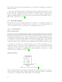
Accelerometer does not measure only acceleration caused by its movement (proper acceleration) as one would probably think, but measures acceleration relative to the free fall. This
means that when the MTx sensor is lying on the table without any movement, it gives approximately 1 g upwards. Because of the free fall the sensor is accelerating upwards relative
to the Earth’s local inertial frame. Einstein stated (Einstein’s Equivalence Principle) that
acceleration caused by movement and force of gravity are indistinguishable. Therefore, the
component of the proper acceleration and the gravitational component are mixed together.
Measured acceleration can be used as an input for more advanced techniques on determining the position of the sensor. But it brings issues how to separate the gravitational
component from the component caused solely by the movement of the sensor. Several
techniques can be applied to accomplish such a task, but this is beyond the scope of this
work. One can for example look it up in [5].
Technical details
Figure 1.1: Accelerometer. From [6].
The device functions in the following way. External acceleration causes the proof mass to
deviate from its neutral position. This is then measured through a change of capacitance
between the proof mass and a fixed frame using a beam structure.
2
1.4.2
Gyroscope
General description
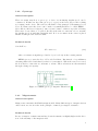
There are many ways how a gyroscope, a device for measuring angular speed can be
constructed. In this case the term gyroscope (or gyro) is used as a jargon, since nothing
is “rotating” in the device. The sensor works rather on the principle of measuring Coriolis
Force. For that reason the device can be made very small (and hence be called MEMS —
Micro-Electro-Mechanical Systems). One very nice feature of this set up is the following.
The sensor does not have to be placed directly at the axis of rotation in order to measure
the angular speed around that particular axis. It does not matter if the sensor is placed
further, it still gives the desired results.
Technical details
Coriolis Force
F = 2mω × v
(1.1)
where m is mass, ω angular speed and v object’s velocity in the rotating system
MEMS gyroscope uses the idea of Foucault Pendulum. But instead of a pendulum a
vibrating mass is used and thus Coriolis force is measured. When the sensor is rotated,
the Coriolis force causes the second frame to vibrate. These vibrations are then measured
through a change in capacity.
Figure 1.2: MEMS gyroscope diagram. Taken from [7]
1.4.3
Magnetometer
General description
Magnetometer measures the Earth’s magnetic field. Many different types of magnetometers
exist, but in our case it works on the principle of anisotropic magneto-resistance.
Technical details
In case of magneto-resistive material its electrical resistance is slightly higher in the direction of the intensity of the magnetic field.
3
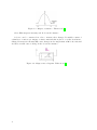
Figure 1.3: Magneto-resistance. Taken from [7]
where H is magnetic intensity and R electrical resistance
A device can be constructed in order to measure these changes. It usually consists of
a thin layer of anisotropic magneto-resistive material that is placed on a silicon substrate.
Changes in magnetic intensity Hy cause changes in the magnetization M of the material
and these in turn cause a change in the electrical resistance.
Figure 1.4: Magnetometer diagram. Taken from [7]
4
Chapter 2
Basics of measurements and
estimation with inertial sensors
Since low-cost inertial sensors are in terms of accuracy very far from their counterparts
used for example in modern aircraft, we proposed several experiments to check the usability
of these sensors for our experiments.
2.1
XSens MTx sensor
We were provided with XSens MTx sensor containing 3-axis accelerometer, gyroscope and
magnetometer. Available sampling frequencies start at hundreds of Hz. The sensor has an
external cache, it can be easily connected to PC via USB and data can be obtained either
in real-time (sample by sample) or in batch-mode (up to 256 samples per batch).
Figure 2.1: XSens MTx Sensor
The MTx is a small and accurate 3DOF Orientation Tracker. It provides drift-free
3D orientation as well as kinematic data: 3D acceleration, 3D rate of turn and 3D earthmagnetic field. For more detailed description (such as concerning sampling frequency)
see [8].
2.2
Connecting with PC
The data flows from the sensor to a cache which is then connected to a PC via USB. Two
modes of obtaining the data exists. One can either set up a direct low level communication
and poll the sensor at the same or higher rate than the sampling frequency and thus get the
data sample by sample (single value polling). Or it is possible to poll the sensor at a lower
5
rate than the sampling frequency and hence obtain the data in batches (buffer polling).
The sensor will manage the right ordering of the data by itself.
2.2.1
Obtaining data through Matlab
The data can be accesed from Matlab through actxserver function. It belongs to the COM
technologies and more specifically ActiveX. In Matlab only the buffer polling method is
available.
The following function creates a handle to the MT-Object.
1
h = actxserver('MotionTracker.CMT');
Then desired sample frequency and output modes are set and we can proceed to the
measurement.
1
2
3
4
time=5; %perform the measurement for 5 seconds
toc
while tic < time
h.cmtGetNextDataBundle()
5
% retrieve the data
[inertialData] = h.cmtDataGetCalData(deviceId);
[eulerAngle] = h.cmtDataGetOriEuler(deviceId);
6
7
8
9
end
For detailed description go to [9], page 48. Code samples are included on the attached
CD.
2.2.2
Obtaining data through LabView
The sensor can also be accessed via LabView environment. I managed to create a script
(both LabView — mtx.vi and executable — ReadLV.exe) for reading accelerometer and
gyroscope data using the buffer polling method. Both can be found on the attached CD.
2.3
Offset
Ideal sensor is supposed to have a zero offset, but unfortunately this is not true for real
devices. What makes matters worse is that the offset also changes all the time. It is somehow dependent on the temperature, orientation of the sensor etc.
2.4
Angular speed integration
If the sensor is rotated in one plane, its orientation can be computed by simply integrating
the output of the gyroscope. We proposed two experiments in order to demonstrate the
influence of noise, offset etc.
In the first one I simply let the sensor lie on a table in a way that its z-axis was pointing
upwards. The sensor was not moving and I integrated the angular speed around the z-axis.
The sample frequency was set to 50 Hz and 2 different methods of integration were used:
rectangular and trapezoidal. The results were compared with the sensor built-in Euler
6
Figure 2.2: Angle estimation — still
angle estimation. Fig. 2.2 shows the obtained results where rect — rectangular approximation, trap — trapezoidal approximation, euler — built-in Euler angle estimation
One can see that within 30 seconds it is already off by 80 degrees. This means that it
is losing the right orientation by approximately 3 degrees per second, so within very short
time this method for estimating orientation of the sensor is totally useless. The results also
show that effects of using different numerical integration method can be neglected. This
suggests that even if the sampling frequency is fairly low, benefits of using more sophisticated method are negligible. Therefore, I will be using only rectangular approximation as
the integration method in the later experiments.
In the second experiment I placed the sensor on a flat surface and rotated it 90 degrees
there and back. Thus, the sensor should end up in exactly the same position as at the
beginning of the experiment. Then I computed the corresponding angle by integrating
the gyro output (z-axis). I also used the results from the previous experiment to estimate
the offset. I did it in a way that I computed the mean of the signal and then subtracted
it from all the signal values in the second experiment. Fig. 2.3 shows the results I obtained.
The results again show that if the computation is not performed using offset estimation,
then over time the correct orientation of the sensor is lost. However, if I first estimate the
offset and use it for the subsequent computation, the results can be even better than the
sensor built-in Euler angle estimation.
7
Figure 2.3: Angle estimation — move
2.5
Acceleration
MTx accelerometers can be used to either estimate speed or position. Thus, we proposed
two experiments to demonstrate that.
2.5.1
Train start
The first experiment took place on the way from Warsaw to Prague by train. The MTx
sensor was positioned with its x-axis in the direction of the tracks and the data were
acquired for two minutes while the train was setting in motion. The acceleration was then
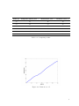
integrated to compute the velocity of the train. The train wagon was equipped with a digital
display that was showing the speed of the train (tachometer). Therefore, the computed
data were compared with the train’s internal system. Table 2.1 shows the results that were
obtained. Computed speed of the train is shown in Fig. 2.4.
As one can see, the results differ slightly. There might be two major reasons for this.
First, the measurement started shortly after the train begun to move, so it could have been
moving at a low speed already. This could explain the difference between the computed
velocity and the tachometer on the first and last two lines of the table 2.1. Concerning the
remaining lines, I can give the following explanation. The tachometer was always showing
the same speed for a longer time and then there was a big jump. So the middle of those
time intervals were used in the table. However, the speed was not changing step-wise, but
was rather gradual, as it is also documented in Fig. 2.4. Therefore, the difference could
have been caused by a wrong synchronisation.
On the other hand, it was astonishing that even though bias and noise must have
corrupted the measured data, the computed speed was quite accurate.
8
Time [s]
Computed speed [kmh−1 ]
Tachometer [kmh−1 ]
Relative error [%]
50
43
48
10
54
46
59
22
63
56
71
21
95
87
94
7
106
98
102
4
110
101
108
6
Table 2.1: Comparing results
Figure 2.4: Train moves off
9
Figure 2.5: Position of the sensor
2.5.2
Distance travelled
The aim of the second experiment was to demonstrate whether it is possible to use the accelerometer as a tool for computing the distance the sensor travels. It was done by double
integrating the acceleration.
The sensor was placed on a flat surface next to a tape (see Fig. 2.5). Its z-axis was
pointing upwards and its x-axis in the opposite direction than the future movement since
then it was easy to move it by holding the cable. First, the sensor was left lying in this
position for 5 seconds which allowed to compute the offset and then it was moved one
meter in a straight line. Fig. 2.6 shows the acceleration that I got, the computed velocity
and the total distance travelled.
.
It can be clearly seen from the measured accelerometer data that the movement started
at cca 0.2 s and finished at 6.2 s. The computed distance at that time is cca 97 cm which
is almost the desired 100 cm. Even though the sensor stopped moving, a non-zero velocity
was indicated and hence the distance was increasing. This was due to a non-zero offset of
the accelerometer.
The reason for such a difference in offset before and after the experiment is most probably the fact that the surface was not as flat as it was assumed. In this way the 1 g that
would normally show up in the z-axis could be projected on the other two axis as well and
disrupt the almost zero offset in the x-axis.
Unlike in the preceding experiments, the results computed using offset were a lot worse
than without offset. When offset was included I did not even get close to the targeted
100 cm.
In general it can be said that double integration increases a lot all the errors such as
offset, noise and so on. Thus, it is not recommended to use this method for measuring
distance without any additional compensation.
10
Figure 2.6: Distance travelled
2.6
3D orientation estimation
Such a simple way of directly integrating the angular speed as described in 2.4 can only
be used for the Euler angle estimation if the sensor stays in one plain (2D). If we want to
estimate the position of the sensor in 3D, the task becomes more complicated. Here it is
not possible to directly integrate the angular speed. One also needs the knowledge of the
previous orientation. The following equation has to be used.
ϕ̇
ωx
θ̇ = R(ϕ, θ, ψ) · ωy
ωz
ψ̇
(2.1)
where ϕ, θ, ψ are Euler angles, R 3 × 3 rotational matrix and ωx , ωy , ωz angular speeds
Such straightforward approach is, however, not normally used. The gyroscope output
contains noise and has offset, so if it is integrated directly, it will yield a huge error as it
is documented in 2.4. Therefore, a more complex approach is applied. As it was described
in 1.4.1, the accelerometer in still position gives 1 g upwards. Thus, from acceleration that
is split between x,y and z-axis it is possible to estimate the position of the sensor. If the
magnitude of the acceleration is smaller or bigger than 1 g, we know that the whole sensor
is accelerating and hence its output cannot be used for orientation estimation. The magnetometer can be used in a similar way. Kalman filter is then applied to decide to what
extent the information from accelerometer and magnetometer should be used to correct
the orientation estimation. [10]
In Xsens Mtx sensor Euler angles are defined as roll, pitch and yaw. It is XYZ Earth
fixed type (subsequent rotation around global X, global Y and global Z axis) [8].
11
Figure 2.7: Euler angles computation
ϕ roll . . . rotation around global x-axis [−180◦ . . . 180◦ ]
θ pitch . . . rotation around global y-axis [−90◦ . . . 90◦ ]
ψ yaw . . . rotation around global z-axis [−180◦ . . . 180◦ ]
Therefore the rotational matrix R can be computed as subsequent rotations around
the x,y and z-axis. Since the definition talks about global axis, the order of multiplication
must be reversed.
R(ϕ, θ, ψ) = Rz (ψ) · Ry (θ) · Rx (ϕ)
(2.2)
where Rz represents rotation around z-axis, Ry represents rotation around y-axis and Rx
represents rotation around x-axis
We designed an experiment to demonstrate the usability of the equation 2.1. It was
implemented together with the definition of Euler angles 2.6 and the results compared with
the sensor built-in computation of Euler angles.
The sensor was placed on a flat surface, its z-axis pointing upwards. Then it was flipped
around y-axis, then 15◦ around the new z-axis there and back, then around the new
x-axis 15◦ there and back and finally back into the original position. The results are shown
in Fig. 2.7
The figure shows that the computed Euler angles fit quite well with the sensor’s built-in
computation. Only roll seems to be influenced a lot by offset. Pavel also found out that
the orientation estimation is valid only when all the singularities are avoided.
The goal of the second experiment was to demonstrate that my algorithm can handle
multiple rotations around the same axis. So I rotated the sensor 3 times around its x-axis.
Fig. 2.8 shows the results that I obtained.
It can be seen that the interval for roll angle is implemented in the same way. However,
the slight disruptions in pitch and yaw caused by the fact that the rotations, which were
not exactly only around x-axis, were amplified in case of my algorithm. It seems like the
sensor’s built-in algorithm includes some sort of compensation.
30◦
12
Figure 2.8: Euler angles computation 2
13
14
Chapter 3
Tremor detection in the laboratory
It is stated in the surveyed literature that the tremor has frequency in the range between 3
to 8 Hz [11]. In order to detect such frequencies in the accelerometer or gyroscope output,
at least double sampling frequency is needed (aliasing theorem). Therefore, the first thing
that had to be done was to double-check the sampling frequency of our sensor, since I
could not find the exact maximum rate in the manual. It was done in a way that more
measurements of the same duration with gradually increasing sampling frequency were
performed. I checked at the end of each experiment whether the number of samples is in
accordance with the duration of the experiment. The following code was used repeatedly.
1
2
3
4
5
duration=1; % the length of the experiment was set to 1 second
sampling frequency=x; % where x is the tested sampling frequency e.g. ...
100 Hz
[X]=measure(duration,sampling frequency); % obtain the data
number of samples=length(X);
[number of samples duration*sampling frequency] %compare the obtained ...
number of samples with the theoretical amount of samples
If number of samples (real amount) was lower than duration*sampling frequency
(theoretical amount), the sampling frequency was decreased. Otherwise, it was increased.
In this way I found out that the sensor can manage sampling frequency up to 210 Hz.
3.1
Off-line detection
The tremor in a given time period can be detected in the following way. Fast Fourier
Transform [12], [13] is computed for the given interval and the highest peak is found. If its
frequency lies between 3 to 8 Hz, tremor is detected. The sensor provides accelerometer,
gyroscope, magnetometer and Euler angle output. Computing FFT for change in orientation turned out not to be a good idea. The specification for bandwidth for accelerometer
is 40 Hz, for gyroscope 30 Hz and for magnetometer 10 Hz [8]. For this reason I decided
not to use the magnetometer since its bandwidth is very close to 8 Hz, which is the upper
bound for the frequency of the tremor. Therefore, I was left with the two remaining ones,
which means 6 outputs in total. Thus, it is necessary to decide which of the sensor outputs
are the most significant ones or which combination of them to use.
The bandwidth also specifies the requirements on the minimal sampling frequency. It
has to be at least two times higher than the largest bandwidth. In our case it is 80 Hz, so
to make it safe I decided to use 100 Hz sampling frequency instead.
15
3.1.1
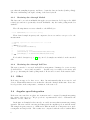
Standard position
We decided to standardize the position in which we will do all the following measurements.
The right forearm is supported by a fixed object (armrest of a chair) and the hand can
move freely. The sensor is then placed on the hand with its z-axis pointing upwards. The
y-axis points in the direction of fingers and the x-axis opposite the thumb.
Figure 3.1: Position of sensor
3.1.2
Measurement
I measured different types of movements in this configuration for one minute: maximum
up and down, rest, normal moves without tremor and simulated tremor. The results are
shown in Fig. 3.2.
Figure 3.2: Different movements
Simulated tremor occurs between 30–40 s and 50–56 s. The results show that the most
significant tremor indicators are acceleration in y and z-axis and angular speed in x and
y-axis.
16
3.1.3
Computing Fast Fourier Transform
Next I used a floating window of size 128 to compute FFT on the selected accelerometer
and gyroscope data. The FFT output was searched for the highest peak and its frequency
was found. The window was then moved by 1 to the right. These frequencies were then
plotted over time. The results are in Fig. 3.3.
Figure 3.3: Frequency estimation
I chose the size 128 of the floating window due to the following reasons. If the sampling
frequency is 100 Hz, then the size of the window corresponds to approximately 1.3 s. If the
window is smaller, then some of the accuracy is lost. If it is larger, then bigger time delay
is introduced. Therefore, 128 seems to be a good compromise.
The FFT algorithm does not use any data that were computed previously. Thus, it
was easy to implement it, but on the other hand, it is a bit slower. So far the speed was
sufficient and thus there was no need to improve it.
I used Hamming window for FFT computation instead of the rectangular one. The
reason is that it should reduce the problem of “spectrum leaking”. This occurs when the
window does not exactly fit to the period of the signal.
3.1.4
Tremor detection
The simple tremor detection algorithm was used. If the frequency was within the range
3 to 8 Hz, it was said that a tremor was detected. So 1 means tremor detected and 0 no
tremor. Results are in Fig. 3.4.
17
Figure 3.4: Tremor detection
I decided to use an AND combination of all the signals to decide whether the tremor
is really detected. This means that all values of the signals must be equal to 1 in order to
say that the tremor is detected. This should suppress false alarms. The results are in Fig.
3.5
Figure 3.5: Final tremor detection
3.1.5
Oscillation filtering
Since there are some oscillations in the detection (close to edges) and some unwanted false
alarms when the patient is in fact at rest, I decided to filter the signal [14]. I chose average
moving window of size 20 to suppress quick oscillations. Fig. 3.6 shows close up of one of
the edges.
18
Figure 3.6: Oscillation filtering
Then the condition for tremor detection can be changed in order to take the filtering
into account. If the value of the signal is below 0.5, it is said that there is no tremor and
if it is higher than 0.5, it is said that the tremor is detected.
3.2
Real-time detection
The results from the section 3.1 were taken into account to design a real-time detection
algorithm. The final program is called tremdet and can be found on the attached CD.
Algorithm 1 tremdet algorithm
upperBound ← 3
. set the upper and lower bound on tremor frequency (in Hz)
lowerBound ← 8
while time < maxT ime do
x ← getN extSample()
. get new data
win ← updateW in(x)
. update floating window
if ¬atRest(win) then
[y, f req] ← f f t(win)
. calculate FFT
maxF req ← f indHighestP eak(y, f req)
. find the highest peak in frequency
if maxF req ≤ upperBound & maxf req ≥ lowerBound then
f lag ← 1
. tremor detected
end if
else
f lag ← 0
. no tremor
end if
end while
The program uses data from y,z-axis accelerometer and x,y-axis gyroscope, thus it operates with 4 signals. The floating window is not a rectangular one, but hamming window
due to the reasons discussed above.
19
There is, however, a huge difference to the off-line detection. Since all the computations
(FFT, finding the highest peak and so on) take some time and in fact are slower than the
time difference between two consecutive samples that is given by the sampling frequency,
the data do not come in sample by sample mode, but in batch-mode.
Therefore, I decided to use a different filter than the floating average of size 20, because
this one would introduce a significant time delay. Instead I use a filter of size 3 working in
the following way. If there are only ones, it is said that tremor is detected. If there are only
zeros, it is said that there is no tremor. If the values are mixed, then nothing is decided
and previous decision about the tremor is used.
Some problems also arise when the hand is not moving (“rest”). There is some noise
in the signal and FFT still detects some frequencies in it that sometimes correspond to
the tremor. Thus, I decided to reduce these false alarms by detecting whether the hand
is moving or not. If the distance between maximum and minimum in the signal is smaller
than a certain threshold, it is said that the hand is not moving at all. Thus, no tremor is
detected and the whole FFT calculation is skipped to save time.
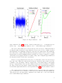
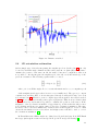
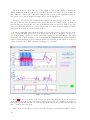
Figure 3.7: Tremdet
Fig. 3.7 shows a screenshot of the tremdet program. The first plot shows the raw data
(rest, simulated tremor, rest, general movement), the second one computed frequency of
the highest peak and the last one both the flag indicating tremor (blue) and the filtered
flag — tremor detection (red).
One can notice in the second plot that the frequency is sometimes 0 Hz for longer
20
periods of time. This corresponds to the “rest” detection i.e. phase when the hand is not
moving. One can also notice that there is a time delay in the tremor detection. This is
caused by the fact that the floating window has to be filled (or emptied) first. The filter
also plays a role which can be observed in the third plot. Finally, it can also been seen
that the filter effectively reduces false alarms.
21
22
Chapter 4
Experiments in the hospital
4.1
Instrumentation available at the Department of Neurology
The next experiments were done at the collaborating Department of Neurology at Karlovo
namesti. We were provided with a goniometer, 3D accelerometer and EMG. Let us first
examine these Noraxon devices.
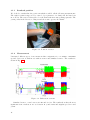
4.1.1
Electromyography
Electromyography (EMG) is a technique that is used for measuring muscle electrical activity. A device called electromyogram measures the electrical potential that is generated by
muscle cells. If the muscle is active, the potential is detected. If it is not active, almost
zero or low potential is detected.
There are two basic types of EMG. Either the electrode is placed by a doctor inside
the muscle using a needle (intramuscular EMG) or the electrode is attached directly to the
skin (surface EMG). The first case provides better results, but on the other hand it could
be quite painful for the patient. Later we will be using the second method, sEMG.
The advantage of sEMG is that it is easy to apply. On the other side, one must ensure
that the electrodes are attached to the right places on the muscle and that they have a
good contact with the skin i.e. by shaving hairs or using special gel.
Noraxon EMG is in this terminology called sEMG.
4.1.2
Accelerometer and goniometer
The difference between MTx accelerometer and Noraxon accelerometer is that in the case
of the Noraxon one a hardware DC filtration can be switched on or off. One can also decide
whether one wants to have a better accuracy in smaller range of values (everything that
exceeds a certain limit is cut off) or whether one wants a wider range of values (but not
so accurate). The first is called 2 g and the second 6 g. Such buttons can be found on the
sensor.
Another difference is the fact that in the case of the Noraxon device the z-axis is oriented
in the other direction comparing to the MTx counterpart.
23
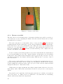
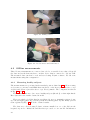
Figure 4.1: EMG position
Figure 4.2: Accelerometer and Goniometer
4.2
Off-line measurements
These Noraxon instruments are connected via cabel to a wearable device that collects all
the data and sends them wireless to another device that is connected to PC via USB.
The measured data can then be read and stored using Polymio software. We did some
measurements using this configuration .
4.2.1
Measuring healthy subjects
The measurements were performed in the standard position defined in 3.1.1. We were using
accelerometer, goniometer and EMG that was placed on the flexor (muskulus flexor carpi
radialis) and extensor (muskulus flexor carpi ulnaris) muscle. The configuration is shown
in Fig. 4.1 and 4.2.
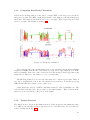
Two measurements were done on two healthy subjects (M and J) on their right hands.
Here I just show the results obtained from M.
They were asked to hold the hand at rest (phase A), move to maximal positions: down,
up, left and right (phase B), perform general movements (phase C) and finally pretend
tremor (phase D). Fig. 4.3 show the obtained results.
The data were collected using Polymio software installed at one of the PC’s in the
hospital, exported to Matlab file and then later processed on our own PC. DC filtration
24
Figure 4.3: M’s Right hand
on the accelerometer was switched on.
The results are again suggesting that the y and z-axis accelerometer output could be
used for tremor detection. However, it turned out that the EMG signal is very much influenced by cable movements. Therefore, it is not sure whether the changes in the signal
are caused by the electrical activity in the muscle or simply by movements of the cables.
Thus, filtering should be applied to remove unwanted signal disturbances. [15]
4.2.2
Measuring patients
Another set of measurements was done on two patients suffering from essential tremor and
on one healthy subject for comparison. Let’s call them P1, P2 and M. Unfortunately, we
were not able to get access to patients with Parkinson tremor.
The measurements were performed in a similar way as in 4.2.1, but there was one
significant difference: the Mtx sensor was positioned on top of the Noraxon accelerometer.
The configuration is shown in Fig. 4.4
The data were collected both with the Polymio software and tremdet program. At the
same time we made videos of the experiments.
The subjects were asked to let the hand freely hang (phase A), move it to the maximal
positions: up, down, left, right (phase B), hold the hand in a horizontal posture (phase
C), make 3 clockwise and 3 counter-clockwise turns (phase D) and finally let it hang freely
again (phase E). Each phase should take approximately 10 s.
This procedure was repeated twice on both hands of P1 and M and twice on the left
hand of P2. We skipped the right hand of P2, because the tremor there was almost unnoticeable. This gives 10 measurements and 10 videos in total. We also have data from both
the Polymio software and some data from the tremdet program.
25
Figure 4.4: Position of the sensors
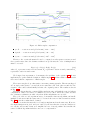
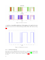
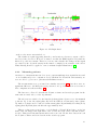
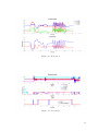
Figure 4.5: P2 Noraxon
P1 had very subtle tremor that was mostly affecting fingers rather than the whole hand.
Therefore, I will show here the data from the healthy subjects M and P2. Both were taken
from the left hand, so the standard position of the sensor had to be adjusted. The x-axis
of the accelerometers pointed in the direction of the thumb. Fig. 4.5 and Fig. 4.6 show
the data obtained from the Noraxon accelerometer (DC filtration switched off, 6 g) and
goniometer. EMG is not shown here, because it is too noisy.
If one looks at the data from the accelerometer, one can notice that there are oscillations
in the case of P2. However, their amplitude was too low to get through the rest detection
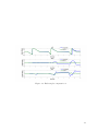
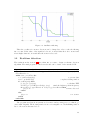
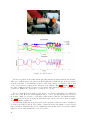
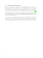
in tremdet. Thus, we decided to relax this condition and re-run the experiment with P2.
Fig. 4.7 shows an excerpt from the measurement. One can see the end of phase B, phase
C and beginning of phase D.
We saw that P2 had the most noticeable tremor in phase C. However, there was almost
no tremor in phase B and D. The results obtained from my algorithm correspond with
this observation. The filter introduced a small time delay in the detection, but successfully
suppressed some false alarms and overlooked tremor.
26
Figure 4.6: M Noraxon
Figure 4.7: P2 tremdet
27
4.3
Real-time measurements
In order to perform real-time computations on the measured signals, it is necessary to read
the samples in batch-mode or ideally one by one. Polymio software does not have this
feature. Therefore, we tried many options of transferring the data to our own PC and
reading them in real-time. My college Pavel Kovář spent a great deal of time focusing on
this, so I will describe it just briefly. For more in-depth explanation, one can look into [16].
First Pavel managed to read the data in real-time in the command line. But later
efforts of sending the data via S-functions to Simulink failed. Sending the data to Matlab
from C environment turned to be slow and complicated. Finally, Pavel managed to read
the data in real-time in LabView.
To get access to the data in real-time one needs two drivers for the Noraxon devices
(nxnusb and myoairo), installed LabView and LabView program that was obtained with
a kind consent from Noraxon. This configuration worked on Windows 7, but not on Windows Vista. Other platforms were not tested. The drivers can be found on the attached CD.
28
Chapter 5
Principles of Functional Electrical
Stimulation and Deep Brain
Stimulation
5.1
Functional Electrical Stimulation
Functional Electrical Stimulation (FES) is a technique used to electrically stimulate muscles. It is mainly used during rehabilitation after an injury to regain movement control
e.g. gait control [17]. It can also be used (combined with regulation techniques) to put a
paralysed patient to a standing position and hold him or her there for a certain time.
Electric current is used as the stimulating medium. Since in this way one is theoretically able to control any muscle movement, this technique can be applied to compensate a
tremor. Of course in reality, this could only be applied to certain muscles. Our main focus
is the forearm.
5.2
Deep Brain Stimulation
Deep Brain Stimulation is a technique used to suppress tremor. It includes a surgical
treatment where a small electrode is precisely put into the brain. The usual targets are
structures within basal ganglia i.e. the subthalamic nucleus (STN) or the internal segment
of the globus pallidus (GPi). A wire then leads to a device located usually under the collarbone. [18].
It is conjectured that every periodical movement in the body is caused by an oscillator
in the brain. Since the tremor has a periodical nature, a region in the brain that is responsible for it can be found and a small electrode is placed there. To simplify it very much, a
noise signal is emitted and thus the particular part of the brain virtually cannot send any
more signals. This then greatly reduces the tremor.
To be more precise, DBS usually functions in a way that it emits high frequency pulses
(around 130 Hz), but its parameters are tuned a bit differently for each patient. However, it
is still unclear, why it works. Recent work [19] shows (based on a mathematical modelling)
that oscillations arise in the brain as the disease progresses. DBS can work in a way that
it reduces time delay and thus stabilizes unstable system [20]. Therefore, the oscillations
are attenuated and the tremor subsides.
29
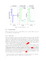
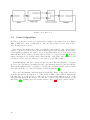
Figure 5.1: Control loop
5.3
Control algorithm
In order to apply the closed-loop feedback tremor regulation, an actuator is needed. Either
DBS or FES can be used for this purpose. Since we did not have access to any of these,
the following is a mere theory.
The tremdet algorithm can be used as a switch for the actuator. One obvious disadvantage of tremor detection based on the inertial sensors is the following. If the tremor
is successfully attenuated, the tremor detection algorithm will not detect any tremor and
thus will shut off the actuator. It will cause the tremor to reappear again [1]. However,
this is a description of P regulator that behaves in this “bang bang” way. A memory and
prediction could be added to this type of detection to create PID regulator.
The EMG signal could also be used for tremor detection. Here filtering has to be applied
in order to face the issues concerning noise and other artefacts caused by cable movements.
Then an algorithm should be designed to separate the electrical activity connected with
the tremor from the one connected with the volitive movements [1].
The control mechanism could work in the following way. Based on the tremor detection
from the inertial sensors, switch on or off the actuator. This could be FES working in the
following way. It would provide a counter move for each tremor influenced move of the
hand and thus suppress the tremor. It could also work in a way that it increases joint
impedance [21]. Or DBS can be used as the actuator. Fig. 5.1 shows a possible scheme.
30
Chapter 6
Conclusion
The key task of this work was to design a real-time tremor detection algorithm and demonstrate that it could be later used as a part of a closed-loop feedback tremor regulation
system.
I got to know the XSens MTx measurement device and together with Pavel we made
some basic experiments with it. I designed a tremor detection algorithm and we demonstrated that it could be used to detect tremor of real patients. We also managed to read
the data from the Noraxon sensors at the collaborating Department of Neurology. With
the help of two skilled doctors, we were able to measure both healthy subjects and subjects
with essential tremor and also record it on video for a possible future use.
However, there is still a lot to be done. First big thing to do, would be using a different
platform for reading sensor data. We were mainly using Matlab environment and that
proved to be very efficient in case of the MTx device. But if we want to read the data from
the Noraxon devices in real-time, there is still a lot to do. Either one can follow what Pavel
did - calling Matlab from C environment or one could start using LabView. We already
demonstrated that it could be used for obtaining data from both the MTx and Noraxon
devices. Thus, a fusion of data from both devices seems to be a next natural step.
Concerning the detection algorithm, our aim was to show that it is possible. So the
algorithm is in no way optimal. One could work further on speeding the FFT computation,
maybe in a way that the algorithm could use some of the already computed data for future
computation as well and do not start from scratch in every loop as it is done in the present
version. Furthermore, the whole detection is based just on the simple information that the
tremor occurs at frequencies between 3 to 8 Hz. Future work could focus on developing
more intelligent detection algorithm based on SVM or Adaboost. However, this would
require collecting a lot more data from both healthy and tremor suffering patients in order
to make such learning possible. If only a small set of data is used, the algorithms could
easily overfit. It means they would detect the specific tremor of that particular patient
rather than the tremor itself.
The EMG measurement itself brought in fact more questions than answers. More work
has to be done in order to properly get rid of all the artefacts caused by cable movements.
Distinguishing the volitional and the non-volitional signal is also a big challenge.
Finally, it would be really exciting to get access to the FES and/or even DBS device
and close the regulation loop. In that case one would have to also focus on developing a
mathematical model of the forearm and hand. In our case we could always use the small
31
MTx device, attach it to our own hand and perform any measurement we wanted. This
would not be possible with a FES device, so one would have to use modelling for developing
and testing the control algorithm. In the case of DBS, a model of the brain tissue would
be required. It would be a very exciting step to an almost unexplored territory.
32
Bibliography
[1] D. Zhang, P. Poignet, F. Widjaja, and W. T. Ang, “Neural oscillator based control for pathological tremor suppression via functional electrical stimulation,” Control
Engineering Practice, vol. 19, no. 1, pp. 74 – 88, 2011.
[2] S. J. Schiff, “Towards model-based control of parkinson’s disease,” Philosophical
Transactions of the Royal Society A: Mathematical, Physical and Engineering Sciences, vol. 368, no. 1918, pp. 2269–2308, 2010.
[3] S. J. Schiff, Neural Control Engineering. The MIT Press, 2012.
[4] E. Růžička and J. Roth, “Parkinsonova nemoc, doporučené postupy,” 2002.
[5] O. Šprdlı́k, Z. Hurák, M. Hoskovcová, O. Ulmanová, and E. Růžička, “Tremor analysis
by decomposition of acceleration into gravity and inertial acceleration using inertial
measurement unit,” Biomedical Signal Processing and Control, vol. 6, no. 3, pp. 269
– 279, 2011.
[6] http://www.efunda.com/formulae/vibrations/sdof_eg_accelerometer.cfm.
[7] P. Ripka, “přednášky a3b38sme senzory a měřenı́,” 2011.
[8] Xsens Technologies, MTi and MTx User Manual and Technical Documentation, 2005.
[9] Xsens Technologies, MT Software Development Kit Documentation, 2005.
[10] M. Rezac and Z. Hurak, “Low-cost inertial estimation unit based on extended kalman
filtering,” 2010.
[11] O. Šprdlı́k, Detection and Estimation of Human Movement Using Inertial Sensors:
Applications in Neurology. PhD thesis, Czech Technical University in Prague, 2012.
[12] H.-J. Bartsch, Matematické vzorce. Academia, 2006.
[13] J. G. Proaklis and D. G. Manolakis, Digital Signal Processing. Prentice Hall, 1996.
[14] G. Chowdhary, S. Srinivasan, and E. N. Johnson, “Frequency domain method for realtime detection of oscillations,” AIAA Journal of Aerospace Computing, Information,
and Communication, vol. 8, pp. 42 – 52, February 2011.
[15] A. Krobot and B. Kolářová, Povrchová electromyografie v klinické praxi. Vydavatelstvı́
Univerzity Palackého v Olomouci, 2011.
[16] P. Kovář, “Potlačovánı́ a detekce třesu u pacientů trpı́cı́ch parkinsonovou chorobou,”
2012.
[17] M. Hruška, “Funkčnı́ elektrická stimulace pro parézu peroneálnı́ho svalu,” Master’s
thesis, Czech Technical University in Prague, 2006.
33
[18] S. Breit, J. B. Schulz, and A.-L. Benabid, “Deep brain stimulation,” Cell and Tissue
Research, vol. 318, pp. 275–288, 2004. 10.1007/s00441-004-0936-0.
[19] A. Nevado-Holgado, J. Terry, and R. Bogacz, “Bifurcation analysis points towards
the source of beta neuronal oscillations in parkinson’s disease,” in Decision and Control and European Control Conference (CDC-ECC), 2011 50th IEEE Conference on,
pp. 6492 –6497, dec. 2011.
[20] M. R. Garcia, M. Verwoerd, B. A. Pearlmutter, P. E. Wellstead, and R. H. Middleton,
“Deep brain stimulation may reduce tremor by preferential blockade of slower axons
via antidromic activation,” in Decision and Control and European Control Conference
(CDC-ECC), 2011 50th IEEE Conference on, pp. 6481 –6486, dec. 2011.
[21] A. Padilha Lanari Bo, C. Azevedo Coste, P. Poignet, C. Geny, and C. Fattal, “On the
Use of FES to Attenuate Tremor by Modulating Joint Impedance,” in CDC-ECC’11:
50th IEEE Conference on Decision and Control and European Control Conference,
vol. Session invitée : Control applications to the electrical treatment of pathological
tremor, (Orlando, Florida, United States), p. 6, Dec. 2011.
34
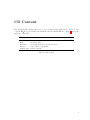
CD Content
The attached CD contains the source codes, measured data with videos, drivers, source
codes in LATEX for generating the PDF file and the final PDF file. Table 1 shows the
structure of the CD.
Directory
Description
Code
Data
Drivers
Thesis
thesis.pdf
source code
measured data
necessary drivers for Noraxon devices
source files for the thesis
bachelor thesis
Table 1: CD Content
I