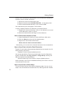
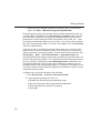
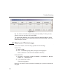
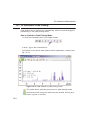
Download User Manual - Pascal-Man

User Manual
Manual for TopSpin 2.1
Version 2.1.1
TopSpin 2.1
Version 2.1.1
User Manual
DONE
INDEX
INDEX
Part Number H9469SA2/10
November 22nd 2007
Bruker software support is available via phone, fax, e-mail or Internet.
Please contact your local office, or directly:
Address:
Phone:
Fax:
E-mail:
WWW:
FTP:
Bruker BioSpin GmbH
Service & Support Department
Silberstreifen
D-76287 Rheinstetten
Germany
+49 (721) 5161 455
+49 (721) 5161 91 455
[email protected]
www.bruker-biospin.com
ftp.bruker.de / ftp.bruker.com
Copyright (C) 2007 by Bruker BioSpin GmbH
All rights reserved. No part of this publication may be reproduced, stored in
a retrieval system, or transmitted, in any form, or by any means without the
prior consent of the publisher.
Product names used are trademarks or registered trademarks of their holders. Words which we have reason to believe constitute registered trademarks are designated as such. However, neither the presence nor the
absence of such designation should be regarded as affecting the legal status of any trademarks.
Bruker Biospin accepts no responsibility for actions taken as a result of use
of this manual.
Computer typset by Bruker BioSpin GmbH, Rheinstetten 2007.
Contents
Chapter 1
Introduction . . . . . . . . . . . . . . . . . . . . . . . . . . . . . . . . . . . . . . . . . I
1.1
1.2
1.3
1.4
1.5
1.6
Chapter 2
About the User Manual . . . . . . . . . . . . . . . . . . . . . . . . . . . . . . . . . . I
Safety Regulations . . . . . . . . . . . . . . . . . . . . . . . . . . . . . . . . . . . . . II
User Manual Conventions . . . . . . . . . . . . . . . . . . . . . . . . . . . . . . . . II
Font Conventions . . . . . . . . . . . . . . . . . . . . . . . . . . . . . . . . . . . . . . II
File/directory Conventions . . . . . . . . . . . . . . . . . . . . . . . . . . . . . . III
User Action Conventions . . . . . . . . . . . . . . . . . . . . . . . . . . . . . . . III
TOPSPIN Overview . . . . . . . . . . . . . . . . . . . . . . . . . . . . . . . . . . . . . III
Functionality . . . . . . . . . . . . . . . . . . . . . . . . . . . . . . . . . . . . . . . . . III
Available Documentation . . . . . . . . . . . . . . . . . . . . . . . . . . . . . . . IV
TOPSPIN license . . . . . . . . . . . . . . . . . . . . . . . . . . . . . . . . . . . . . . . V
TopSpin program versions. . . . . . . . . . . . . . . . . . . . . . . . . . . . . . . V
................................................... V
Getting Started . . . . . . . . . . . . . . . . . . . . . . . . . . . . . . . . . . . . . 19
2.1
2.2
2.3
2.4
2.5
2.6
2.7
2.8
2.9
2.10
2.11
2.12
2.13
2.14
Startup TOPSPIN . . . . . . . . . . . . . . . . . . . . . . . . . . . . . . . . . . . . . . .19
Configuration . . . . . . . . . . . . . . . . . . . . . . . . . . . . . . . . . . . . . . . . . 20
How to Display Spectra . . . . . . . . . . . . . . . . . . . . . . . . . . . . . . . . .21
How to Open Data from the Menu . . . . . . . . . . . . . . . . . . . . . . . . 21
How to Open Data from the Browser . . . . . . . . . . . . . . . . . . . . . . 21
How to Define Alias Names for Data . . . . . . . . . . . . . . . . . . . . . .22
How to Open Data in Archive Data Directories . . . . . . . . . . . . . . 22
How to Open Data in Other Ways . . . . . . . . . . . . . . . . . . . . . . . . 22
How to Expand a Spectral Region. . . . . . . . . . . . . . . . . . . . . . . . . 23
How to Display Peaks, Integrals, ... together with the Spectrum. . 23
How to Display Projections/1D Spectra with 2D Spectra . . . . . . . 23
How to Superimpose Spectra in Multiple Display . . . . . . . . . . . . . 24
How to Print or Export the Contents of a Data Window . . . . . . . . 24
How to Print Data . . . . . . . . . . . . . . . . . . . . . . . . . . . . . . . . . . . . . 24
How to Copy a Data Window to Clipboard . . . . . . . . . . . . . . . . . . 25
How to Store (Export) a Data Window as Graphics File . . . . . . . 25
How to Process Data. . . . . . . . . . . . . . . . . . . . . . . . . . . . . . . . . . . 25
How to Archive Data . . . . . . . . . . . . . . . . . . . . . . . . . . . . . . . . . . .27
How to Import NMR Data Stored in Special Formats . . . . . . . . . .28
How to Fit Peaks and Deconvolve Overlapping Peaks . . . . . . . . . 28
How to Compute Fids by Simulating Experiments . . . . . . . . . . . . 29
How to Add Your Own Functionalities . . . . . . . . . . . . . . . . . . . . . . 29
How to Create Macros . . . . . . . . . . . . . . . . . . . . . . . . . . . . . . . . . 29
3
Chapter 3
How to Create AU (automation) Programs . . . . . . . . . . . . . . . . . . 29
How to Create Python Programs . . . . . . . . . . . . . . . . . . . . . . . . . 30
2.15 How
to Automate Data Acquisition . . . . . . . . . . . . . . . . . . . . . . . . 30
INDEX
The TOPSPIN Interface . . . . . . . . . . . . . . . . . . . . . . . . . . . . . . . . 31
3.1
3.2
3.3
3.4
3.5
3.6
3.7
3.8
Chapter 4
Trouble Shooting . . . . . . . . . . . . . . . . . . . . . . . . . . . . . . . . . . . 49
4.1
4.2
4.3
4.4
4.5
Chapter 5
General Tips and Tricks . . . . . . . . . . . . . . . . . . . . . . . . . . . . . . . . 49
History, Log Files, Spooler Reports, Stack Trace . . . . . . . . . . . . . 49
How to Show or Kill TOPSPIN processes . . . . . . . . . . . . . . . . . . . . 53
What to do if TOPSPIN hangs . . . . . . . . . . . . . . . . . . . . . . . . . . . . .54
How to Restart User Interface during Acquisition . . . . . . . . . . . . . 55
Dataset Handling . . . . . . . . . . . . . . . . . . . . . . . . . . . . . . . . . . . . 57
5.1
5.2
4
The
Topspin Window
. . . . . . . . . . . . . . . . . . . . . . . . . . . . . . . . . . . 31
INDEX
DONE
How to Use Multiple Data Windows . . . . . . . . . . . . . . . . . . . . . . . 32
How to Use the Menu bar . . . . . . . . . . . . . . . . . . . . . . . . . . . . . . . 33
How to Use the Upper Toolbar (1D data) . . . . . . . . . . . . . . . . . . . 34
How to Use the Lower Toolbar (1D data) . . . . . . . . . . . . . . . . . . . 35
Command Line Usage. . . . . . . . . . . . . . . . . . . . . . . . . . . . . . . . . . 37
How to Put the Focus in the Command Line . . . . . . . . . . . . . . . .37
How to Retrieve Previously Entered Commands . . . . . . . . . . . . .37
How to Change Previously Entered Commands . . . . . . . . . . . . . 38
How to Enter a Series of Commands . . . . . . . . . . . . . . . . . . . . . . 38
Command Line History . . . . . . . . . . . . . . . . . . . . . . . . . . . . . . . . . 38
Starting TOPSPIN commands from a Command Prompt. . . . . . . . . 39
Function Keys and Control Keys . . . . . . . . . . . . . . . . . . . . . . . . . .40
Help in Topspin . . . . . . . . . . . . . . . . . . . . . . . . . . . . . . . . . . . . . . . 44
How to Open Online Help documents . . . . . . . . . . . . . . . . . . . . . 45
How to Get Tooltips . . . . . . . . . . . . . . . . . . . . . . . . . . . . . . . . . . .45
How to Get Help on Individual Commands . . . . . . . . . . . . . . . . . 46
How to Use the Command Index . . . . . . . . . . . . . . . . . . . . . . . . . 46
User Defined Functions Keys . . . . . . . . . . . . . . . . . . . . . . . . . . . . 47
How to Open Multiple TOPSPIN Interfaces . . . . . . . . . . . . . . . . . . . 47
The Topspin Browser. . . . . . . . . . . . . . . . . . . . . . . . . . . . . . . . . . . 57
How to Open the Browser in a separate window . . . . . . . . . . . . .61
How to Put the Focus in the Browser . . . . . . . . . . . . . . . . . . . . . . 61
How to Select Folders in the Browser . . . . . . . . . . . . . . . . . . . . . 62
How to Expand/Collapse a Folder in the Browser . . . . . . . . . . . . 62
How to Show/Hide Pulse program and Title in the browser . . . . . 62
How to Show Dataset Dates in the Browser . . . . . . . . . . . . . . . .63
How to change the default Top Level Data Directory . . . . . . . . . . 64
How to Add, Remove or Interpret Alias Names . . . . . . . . . . . . . . 64
Creating Data . . . . . . . . . . . . . . . . . . . . . . . . . . . . . . . . . . . . . . . . 65
5.3
5.4
5.5
5.6
5.7
5.8
Chapter 6
How to Create a New Dataset . . . . . . . . . . . . . . . . . . . . . . . . . . . 65
Opening Data . . . . . . . . . . . . . . . . . . . . . . . . . . . . . . . . . . . . . . . . 66
How
to Open Data Windows Cascaded . . . . . . . . . . . . . . . . . . . .67
INDEX
How to Open Data from the Browser . . . . . . . . . . . . . . . . . . . . . . 68
How
to Automatically
Select the first expno/procno of a dataset . 69
INDEX
DONE
How to Open Data from the Topspin menu . . . . . . . . . . . . . . . . . 70
How to Open Data from the Explorer, Konqueror or Nautilus . . .72
How to Open Data from the Command Line . . . . . . . . . . . . . . . .73
How to Open Special Format Data . . . . . . . . . . . . . . . . . . . . . . . . 75
How to Open a ZIP or JCAMP-DX file
from the Windows Explorer . . . . . . . . . . . . . 76
Saving/Copying Data. . . . . . . . . . . . . . . . . . . . . . . . . . . . . . . . . . . 77
How to Save or Copy Data . . . . . . . . . . . . . . . . . . . . . . . . . . . . . . 77
How to Save an Entire Dataset . . . . . . . . . . . . . . . . . . . . . . . . . . 78
How to Save Processed Data . . . . . . . . . . . . . . . . . . . . . . . . . . . 78
How to Save Acquisition Data . . . . . . . . . . . . . . . . . . . . . . . . . . . 78
How to Save Processed Data as Pseudo Raw Data . . . . . . . . . .78
Deleting Data. . . . . . . . . . . . . . . . . . . . . . . . . . . . . . . . . . . . . . . . . 79
How to Delete a Specific Dataset . . . . . . . . . . . . . . . . . . . . . . . . . 79
How to Delete Types of Datasets . . . . . . . . . . . . . . . . . . . . . . . . . 79
Renaming Data . . . . . . . . . . . . . . . . . . . . . . . . . . . . . . . . . . . . . . .79
How to Rename a Specific Dataset . . . . . . . . . . . . . . . . . . . . . . . 79
Searching/Finding Data . . . . . . . . . . . . . . . . . . . . . . . . . . . . . . . . .82
How to Find Data . . . . . . . . . . . . . . . . . . . . . . . . . . . . . . . . . . . . . 82
How to Display one of the Found Datasets . . . . . . . . . . . . . . . . . 83
Handling Data Files . . . . . . . . . . . . . . . . . . . . . . . . . . . . . . . . . . . . 85
How to List/Open the Current Dataset Files . . . . . . . . . . . . . . . . . 85
How to List/Open the current Dataset Files
in the Windows Explorer . . . . . . . . . . . . . . . . 86
Parameter Handling . . . . . . . . . . . . . . . . . . . . . . . . . . . . . . . . . 89
6.1
6.2
Processing Parameters . . . . . . . . . . . . . . . . . . . . . . . . . . . . . . . . .89
How to Set a Processing Parameter from the Command Line . . . 89
How to Set Processing Parameters from the Parameter Editor . . 90
How to Undo the Last Processing Parameter Change . . . . . . . . . 92
How to Display Processing Status Parameters . . . . . . . . . . . . . . 92
How to Switch to Maxent parameters . . . . . . . . . . . . . . . . . . . . . . 92
How to Change Processed Data Dimensionality . . . . . . . . . . . . . 92
Acquisition Parameters . . . . . . . . . . . . . . . . . . . . . . . . . . . . . . . . .93
How to Set Acquisition Parameters . . . . . . . . . . . . . . . . . . . . . . . 93
How to Set an Acquisition Parameter from the Command Line . . 93
How to Set Acquisition Parameters from the Parameter Editor . . 94
5
How to Undo the Last Acquisition Parameter Change . . . . . . . . . 96
How to Set Pulse Program Parameters . . . . . . . . . . . . . . . . . . . .96
How to Display Acquisition Status INDEX
Parameters . . . . . . . . . . . . . . 96
How to Get Probehead/Solvent dependent Parameters . . . . . . . 96
How to Change Acquisition
. . . . . . . . . . . . .97
DONE Data Dimensionality
INDEX
How to Set Lock Parameters . . . . . . . . . . . . . . . . . . . . . . . . . . . . 97
How to Set Routing Parameters . . . . . . . . . . . . . . . . . . . . . . . . . .97
Chapter 7
Data Processing . . . . . . . . . . . . . . . . . . . . . . . . . . . . . . . . . . . . 99
7.1
7.2
7.3
7.4
Chapter 8
Printing/Exporting Data . . . . . . . . . . . . . . . . . . . . . . . . . . . . . 109
8.1
8.2
Chapter 9
Printing/plotting Data . . . . . . . . . . . . . . . . . . . . . . . . . . . . . . . . . . 109
How to Print/Plot from the Menu . . . . . . . . . . . . . . . . . . . . . . . . 109
How to Plot Data from the Processing guide . . . . . . . . . . . . . . .111
How to Plot Data with the Plot Editor . . . . . . . . . . . . . . . . . . . . . 112
How to Print the Integral list . . . . . . . . . . . . . . . . . . . . . . . . . . . . 112
How to Print the Peak list . . . . . . . . . . . . . . . . . . . . . . . . . . . . . . 112
Exporting Data. . . . . . . . . . . . . . . . . . . . . . . . . . . . . . . . . . . . . . . 113
How to Copy data to Other Applications . . . . . . . . . . . . . . . . . . 113
How to Store (Export) a Data Window as Graphics File . . . . . . 114
1D Display . . . . . . . . . . . . . . . . . . . . . . . . . . . . . . . . . . . . . . . . 115
9.1
9.2
9.3
9.4
6
Interactive Processing . . . . . . . . . . . . . . . . . . . . . . . . . . . . . . . . . . 99
How to Process Data with Single Commands . . . . . . . . . . . . . . . 99
How to Process data with Composite Commands . . . . . . . . . . . 100
Semi-automatic Processing. . . . . . . . . . . . . . . . . . . . . . . . . . . . . 100
How to Use the 1D Processing Dialog . . . . . . . . . . . . . . . . . . . . 100
How to Use the Processing Guide in Automatic mode . . . . . . . . 101
How to Use the Processing Guide in Interactive mode . . . . . . . 103
Processing Data with AU programs . . . . . . . . . . . . . . . . . . . . . . 103
Serial Processing . . . . . . . . . . . . . . . . . . . . . . . . . . . . . . . . . . . . 104
The 1D Data Window . . . . . . . . . . . . . . . . . . . . . . . . . . . . . . . . . 115
Displaying one Dataset in Multiple windows . . . . . . . . . . . . . . . . 116
How to Reopen a Dataset in a Second/Third etc. Window . . . . 116
How to Rescale or Shift one Dataset in Multiple windows . . . . . 117
Changing the Display of a 1D Spectrum or FID . . . . . . . . . . . . . 118
How to Change the Vertical Scaling of the FID or Spectrum . . . 118
How to Smoothly Change the Vertical Scaling
of the FID/Spectrum . . . . . . . . . . . . . . . 118
How to Change the Horizontal Scaling of the FID or Spectrum . 119
How to Shift a Spectral Region to the Left or to the Right . . . . . 120
How to Shift the Spectrum Up or Down . . . . . . . . . . . . . . . . . . . 120
Using the Tab bar . . . . . . . . . . . . . . . . . . . . . . . . . . . . . . . . . . . . 121
How to Display the Spectrum . . . . . . . . . . . . . . . . . . . . . . . . . . . 121
9.5
9.6
9.7
9.8
How to Set Processing Parameters . . . . . . . . . . . . . . . . . . . . . . 122
How to Set Acquisition Parameters . . . . . . . . . . . . . . . . . . . . . . 123
How
to Edit the Title . . . . . . . . . . . . . . . . . . . . . . . . . . . . . . . . . . 124
INDEX
How to Edit the Pulse Program . . . . . . . . . . . . . . . . . . . . . . . . . 125
How
to Display the
Peak list . . . . . . . . . . . . . . . . . . . . . . . . . . . . 125
INDEX
DONE
How to Display the Integral list . . . . . . . . . . . . . . . . . . . . . . . . . . 134
How to view Sample Information . . . . . . . . . . . . . . . . . . . . . . . . 142
How to Open the Jmol Molecule Structure Viewer . . . . . . . . . . . 143
How to Display the FID . . . . . . . . . . . . . . . . . . . . . . . . . . . . . . . .145
1D Display Options . . . . . . . . . . . . . . . . . . . . . . . . . . . . . . . . . . . 145
How to Toggle between Hertz and ppm Axis Units . . . . . . . . . . 145
How to Switch on/off the Spectrum Overview display . . . . . . . .145
How to Switch Y-axis Display . . . . . . . . . . . . . . . . . . . . . . . . . . . 146
Show Display Properties/Regions/Files . . . . . . . . . . . . . . . . . . . 146
How to Superimpose the Cursor Information . . . . . . . . . . . . . . . 148
How to Superimpose the Title on the Spectrum . . . . . . . . . . . . . 149
How to Superimpose the main Status Parameters
on the Spectrum . . . . . . . . . . . . . . 149
How to Superimpose the Integral Trails/Labels
on the Spectrum . . . . . . . . . . . . . . . 149
How to Superimpose Peak Labels on the Spectrum . . . . . . . . .149
How to Show Peak Annotations on the Spectrum . . . . . . . . . . . 150
How to Show Individual Data Points of the Spectrum . . . . . . . .150
How to Superimpose the Electronic Signature on the Spectrum 150
How to Display the Main Dataset Properties . . . . . . . . . . . . . . .150
How to Display a List of Files of a Dataset . . . . . . . . . . . . . . . . . 151
Saving Display Region . . . . . . . . . . . . . . . . . . . . . . . . . . . . . . . . 154
Synchronize Visible Region of all Data Windows . . . . . . . . . . . . 155
Chapter 10 2D Display . . . . . . . . . . . . . . . . . . . . . . . . . . . . . . . . . . . . . . . . 157
10.1 The 2D Data Window . . . . . . . . . . . . . . . . . . . . . . . . . . . . . . . . . 157
10.2 Changing the Display of a 2D spectrum . . . . . . . . . . . . . . . . . . . 158
How to Change the Intensity Scaling (contour levels) . . . . . . . .158
How to Smoothly Change the Vertical Scaling (contour levels) . 159
How to Display a Contour Levels Bar in the Data Window . . . . 159
How to Switch on/off Square 2D layout . . . . . . . . . . . . . . . . . . . 160
How to Zoom a 2D spectrum in/out . . . . . . . . . . . . . . . . . . . . . . 161
How to Shift a Spectral Region in the F2 direction (left/right) . . . 162
How to Shift a Spectral Region in the F1 direction (up/down) . .162
10.3 Show Display Properties/Regions/Files . . . . . . . . . . . . . . . . . . . 162
10.4 Using the Tab bar . . . . . . . . . . . . . . . . . . . . . . . . . . . . . . . . . . . . 165
How to Set Processing Parameters . . . . . . . . . . . . . . . . . . . . . . 165
7
How to Set Acquisition Parameters . . . . . . . . . . . . . . . . . . . . . . 165
How to Display the Peak list . . . . . . . . . . . . . . . . . . . . . . . . . . . . 166
How to Display the Integral list . . .INDEX
. . . . . . . . . . . . . . . . . . . . . . . 167
How to Display the FID . . . . . . . . . . . . . . . . . . . . . . . . . . . . . . . .169
10.5 2D Display OptionsDONE
. . . . . . . . . . . INDEX
. . . . . . . . . . . . . . . . . . . . . . . . 169
How to Switch between Hertz and ppm Axis Units
in F2 and F1 . . . . . . . . . . . . . . . 169
How to Switch on/off the Spectrum Overview display . . . . . . . .169
How to Switch on/off the Projection display . . . . . . . . . . . . . . . . 170
How to Switch on/off the Grid display . . . . . . . . . . . . . . . . . . . . . 172
How to Display a 2D Spectrum in Contour Mode . . . . . . . . . . . .173
How to Set the 2D Contour Levels . . . . . . . . . . . . . . . . . . . . . . . 174
How to Store interactively set Contour Levels . . . . . . . . . . . . . . 175
How to Display a 2D spectrum in Pseudo Color Mode . . . . . . . 176
How to Display a 2D Spectrum in Oblique Mode . . . . . . . . . . . .176
How to Rotate a 2D Spectrum in Oblique Mode . . . . . . . . . . . . 178
How to Switch between Displaying Positive
and Negative levels . . . . . . . . . . . . . . . . . 178
Chapter 11 nD Display . . . . . . . . . . . . . . . . . . . . . . . . . . . . . . . . . . . . . . . . 179
11.1
11.2
11.3
11.4
11.5
Display Planes of 3D Data . . . . . . . . . . . . . . . . . . . . . . . . . . . . . 179
How to Switch to 2D Plane Display . . . . . . . . . . . . . . . . . . . . . . 180
How to Display various Plane Orientations . . . . . . . . . . . . . . . . 180
How to Display various Plane Positions (numbers) . . . . . . . . . . 181
3D Cube Display Mode . . . . . . . . . . . . . . . . . . . . . . . . . . . . . . . .182
How to Display the 3D Cube . . . . . . . . . . . . . . . . . . . . . . . . . . . 182
How to Rotate the 3D Cube . . . . . . . . . . . . . . . . . . . . . . . . . . . . 182
How to Scale Up/Down the 3D Cube . . . . . . . . . . . . . . . . . . . . . 183
How to Reset the Cube Size and Orientation . . . . . . . . . . . . . . . 183
How to Switch Depth Cueing on/off . . . . . . . . . . . . . . . . . . . . . . 183
How to Display a Cube Front or Side view . . . . . . . . . . . . . . . . . 183
nD parameter display . . . . . . . . . . . . . . . . . . . . . . . . . . . . . . . . . 183
nD Fid Display . . . . . . . . . . . . . . . . . . . . . . . . . . . . . . . . . . . . . . . 185
nD Peak and Integral Display . . . . . . . . . . . . . . . . . . . . . . . . . . . 186
Chapter 12 1D Interactive Manipulation . . . . . . . . . . . . . . . . . . . . . . . . . . 189
12.1 1D Interactive Window multiplication. . . . . . . . . . . . . . . . . . . . . . 189
How to Switch to Window Multiplication Mode . . . . . . . . . . . . . . 189
12.2 1D Interactive Phase Correction . . . . . . . . . . . . . . . . . . . . . . . . .191
How to Switch to Phase Correction Mode . . . . . . . . . . . . . . . . . 191
How to Perform a Typical 1D Interactive Phase Correction . . . . 192
How to Set the Phase Pivot Point . . . . . . . . . . . . . . . . . . . . . . . 192
How to Perform Default Zero Order Phase Correction . . . . . . . . 193
8
How to Perform Interactive Zero Order Phase Correction . . . . . 193
How to Perform Interactive First Order Phase Correction . . . . . 193
How
to Perform 90, -90 or 180° Zero Order Phase Correction . 193
INDEX
How to Reset the Phase to the Original Values . . . . . . . . . . . . . 193
How
to Change the
Mouse Sensitivity . . . . . . . . . . . . . . . . . . . . 194
INDEX
DONE
How to Return from Phase Correction Mode with/without Save 194
12.3 1D Interactive Integration . . . . . . . . . . . . . . . . . . . . . . . . . . . . . . 194
How to Switch to Integration Mode . . . . . . . . . . . . . . . . . . . . . . . 195
How to Define Integral Regions . . . . . . . . . . . . . . . . . . . . . . . . . 196
How to Select/Deselect Integral Regions . . . . . . . . . . . . . . . . . . 197
How to Read Integral Regions from Disk . . . . . . . . . . . . . . . . . . 198
How to Perform Interactive Bias and Slope Correction . . . . . . . 199
How to Set the Limit for Bias Determination . . . . . . . . . . . . . . . . 200
How to Change the Mouse Sensitivity . . . . . . . . . . . . . . . . . . . . 200
How to Calibrate/Normalize Integrals . . . . . . . . . . . . . . . . . . . . . 200
How to Scale Integrals with respect to Different Spectra . . . . . .201
How to Delete Integral Regions from the Display . . . . . . . . . . . .201
How to Scale Selected Integrals . . . . . . . . . . . . . . . . . . . . . . . . 202
How to Move the Integral Trails Up/Down . . . . . . . . . . . . . . . . . 203
How to Cut Integral Regions . . . . . . . . . . . . . . . . . . . . . . . . . . . 203
How to Save Integral Regions . . . . . . . . . . . . . . . . . . . . . . . . . . 203
How to Undo the Last Region Operation . . . . . . . . . . . . . . . . . . 204
How to Return from the Integration Mode with/without Save . . . 204
12.4 1D Interactive Calibration . . . . . . . . . . . . . . . . . . . . . . . . . . . . . . 205
How to Switch to Calibration Mode . . . . . . . . . . . . . . . . . . . . . . 205
How to Calibrate a Spectrum Interactively . . . . . . . . . . . . . . . . . 206
12.5 1D Multiple Display . . . . . . . . . . . . . . . . . . . . . . . . . . . . . . . . . . . 207
How Switch to Multiple Display Mode and
Read Multiple Spectra . . . . . . . . .207
How to Select/Deselect Datasets . . . . . . . . . . . . . . . . . . . . . . . . 209
How to Remove a Dataset from Multiple Display . . . . . . . . . . . .210
How to Display the Sum or Difference Spectra . . . . . . . . . . . . . 210
How to Save the Sum or Difference Spectra . . . . . . . . . . . . . . .210
How to Display the Next/Previous Name/Expno . . . . . . . . . . . . 211
How to Toggle between Superimposed and Stacked Display . .211
How to Shift and Scale Individual Spectra . . . . . . . . . . . . . . . . . 212
How to move the selected spectrum one place up/down . . . . . .213
How to Switch on/off the Display of Datapaths
and Scaling Factors . . . . . . . . . . . 214
How to Return from Multiple Display mode . . . . . . . . . . . . . . . . 214
How to Set the Colors of the 1st, 2nd, .. Dataset . . . . . . . . . . . . 214
9
12.6 1D Interactive Baseline Correction . . . . . . . . . . . . . . . . . . . . . . . 214
How to Switch to Baseline Correction Mode . . . . . . . . . . . . . . .214
How to Perform Polynomial Baseline
Correction . . . . . . . . . . . .215
INDEX
How to Perform Sine Baseline Correction . . . . . . . . . . . . . . . . . 216
How to Perform Exponential
Correction . . . . . . . . . . . 216
DONE Baseline
INDEX
How to Preview the Baseline Corrected Spectrum . . . . . . . . . . 216
How to Reset the Baseline Correction Line . . . . . . . . . . . . . . . . 217
How to Change the Mouse Sensitivity . . . . . . . . . . . . . . . . . . . . 217
How to Save the Baseline Correction and/or Return . . . . . . . . .217
How to Perform Cubic Spline Baseline correction . . . . . . . . . . . 218
How to Delete Spline Baseline Points from the screen . . . . . . . 219
How to Return from Cubic Spline Baseline mode
with/without Save . . . . . . . . . . . .219
12.7 1D Interactive Peak Picking . . . . . . . . . . . . . . . . . . . . . . . . . . . .220
How to Switch to Peak Picking Mode . . . . . . . . . . . . . . . . . . . . . 220
How to Define New Peak Picking Ranges . . . . . . . . . . . . . . . . . 221
How to Change Peak Picking Ranges . . . . . . . . . . . . . . . . . . . . 221
How to Pick Peaks in Peak Picking Ranges only . . . . . . . . . . . .221
How to Delete all Peak Picking Ranges . . . . . . . . . . . . . . . . . . .222
How to Define Peaks Manually . . . . . . . . . . . . . . . . . . . . . . . . . 222
How to Pick Peaks Semi-Automatically . . . . . . . . . . . . . . . . . . . 222
How to Delete Peaks from the Peak List . . . . . . . . . . . . . . . . . . 223
How to Return from Peak Picking Mode with/without Save . . . . 224
Chapter 13 2D Interactive Manipulation . . . . . . . . . . . . . . . . . . . . . . . . . . 225
13.1 2D Interactive Phase Correction . . . . . . . . . . . . . . . . . . . . . . . . .225
How to Switch to 2D Interactive Phase Correction . . . . . . . . . . . 225
How to Perform a Typical 2D Interactive Phase Correction . . . . 226
How to Scale or Shift Individual Rows/Columns . . . . . . . . . . . . 229
How to Perform Smooth Phase Correction . . . . . . . . . . . . . . . . 230
How to Perform 90, -90 or 180° Zero Order Phase Correction . 231
How to Reset the Phase to the Original Values . . . . . . . . . . . . . 231
How to Change the Mouse Sensitivity . . . . . . . . . . . . . . . . . . . . 231
How to Show the Next/Previous Row or Column . . . . . . . . . . . .231
How to Arrange Rows or Columns . . . . . . . . . . . . . . . . . . . . . . . 232
How to Return from Multi-1D Phase to 2D Phase Display . . . . . 232
How to Return from 2D Phase Mode . . . . . . . . . . . . . . . . . . . . . 232
13.2 2D Interactive Integration . . . . . . . . . . . . . . . . . . . . . . . . . . . . . . 232
How to Move an Integral region . . . . . . . . . . . . . . . . . . . . . . . . .237
How to Copy an Integral region . . . . . . . . . . . . . . . . . . . . . . . . . 237
How to Delete all Integral Regions . . . . . . . . . . . . . . . . . . . . . . . 237
How to Read/Import Integral Regions . . . . . . . . . . . . . . . . . . . . 237
10
How to Save/Export Integral Regions . . . . . . . . . . . . . . . . . . . . 238
How to Return from 2D Integration mode . . . . . . . . . . . . . . . . . 238
13.3 2D
Multiple Display and Row/Column Handling . . . . . . . . . . . . . 238
INDEX
How Switch to Multiple Display mode and
Read Multiple Spectra . . . . . . . . .238
INDEX
DONE
How to Align Multiple 2D Spectra . . . . . . . . . . . . . . . . . . . . . . . . 241
How to Display the Next/Previous Name/Expno . . . . . . . . . . . . 241
How to Scan Rows/Columns . . . . . . . . . . . . . . . . . . . . . . . . . . . 242
How to Grab a Row/Column . . . . . . . . . . . . . . . . . . . . . . . . . . . . 242
How to Show the Next/Previous Row or Column . . . . . . . . . . . .243
How to Move the Selected Dataset Up/Down in Dataset List . .244
How to Extract a Row/Column . . . . . . . . . . . . . . . . . . . . . . . . . . 244
How to Copy Contour Levels from First to Other Spectra . . . . . 245
How to Switch on/off 2D contour display . . . . . . . . . . . . . . . . . . 245
How to Position the Baseline of the Row/Column . . . . . . . . . . . 245
13.4 2D Interactive Calibration . . . . . . . . . . . . . . . . . . . . . . . . . . . . . . 246
How to Switch to 2D Calibration mode . . . . . . . . . . . . . . . . . . . . 246
How to Perform 2D Calibration . . . . . . . . . . . . . . . . . . . . . . . . . . 247
13.5 2D Chemical Shift Distance Measurement . . . . . . . . . . . . . . . . . 247
How to Measure a 2D Chemical Shift Distance . . . . . . . . . . . . . 247
Chapter 14 Data Window Handling . . . . . . . . . . . . . . . . . . . . . . . . . . . . . . 249
14.1 Data Windows . . . . . . . . . . . . . . . . . . . . . . . . . . . . . . . . . . . . . . . 249
How to Move a Data Window . . . . . . . . . . . . . . . . . . . . . . . . . . . 250
How to Resize a Data Window . . . . . . . . . . . . . . . . . . . . . . . . . . 250
How to Select (activate) a Data Window . . . . . . . . . . . . . . . . . . 251
How to Open a New empty Data Window . . . . . . . . . . . . . . . . . 252
How to Arrange Data Windows . . . . . . . . . . . . . . . . . . . . . . . . . 252
How to Iconify (minimize) a Data Window . . . . . . . . . . . . . . . . . 254
How to De-iconify a Data Window . . . . . . . . . . . . . . . . . . . . . . . 255
How to Maximize a Data Window . . . . . . . . . . . . . . . . . . . . . . . . 255
How to Restore the Size and Position of a Data Window . . . . . 255
How to Close a Data Window . . . . . . . . . . . . . . . . . . . . . . . . . . . 255
How to Iconify all Data Windows . . . . . . . . . . . . . . . . . . . . . . . . 256
How to Maximize all Data Windows . . . . . . . . . . . . . . . . . . . . . . 256
How to Activate the Next Data Window . . . . . . . . . . . . . . . . . . . 256
14.2 Window Layouts . . . . . . . . . . . . . . . . . . . . . . . . . . . . . . . . . . . . . 256
How to Save the Current Window Layout . . . . . . . . . . . . . . . . . 256
How to Read a Window Layout . . . . . . . . . . . . . . . . . . . . . . . . . 256
How to Swap Data Windows . . . . . . . . . . . . . . . . . . . . . . . . . . . 257
How to Toggle Window Decoration . . . . . . . . . . . . . . . . . . . . . . 257
11
Chapter 15 Analysis . . . . . . . . . . . . . . . . . . . . . . . . . . . . . . . . . . . . . . . . . . 259
15.1 Introduction . . . . . . . . . . . . . . . . . . . . . . . . . . . . . . . . . . . . . . . . .259
15.2 Chemical Shift Distance Measurement . . . . . . . . . . . . . . . . . . . 260
How to Measure a Chemical Shift Distance . . . . . . . . . . . . . . . . 260
15.3 1D Signal to Noise Calculation . . . . . . . . . . . . . . . . . . . . . . . . . . 260
How to Perform Interactive S/N Calculation . . . . . . . . . . . . . . . . 260
How to Delete the Signal Region or Noise Region . . . . . . . . . . . 262
How to Edit the Limits of the Signal Region or Noise Region . .262
How to Change Width of the Signal Region or Noise Region . .262
15.4 Relaxation Analysis . . . . . . . . . . . . . . . . . . . . . . . . . . . . . . . . . . . 263
Chapter 16 Acquisition . . . . . . . . . . . . . . . . . . . . . . . . . . . . . . . . . . . . . . . 271
16.1
16.2
16.3
16.4
16.5
16.6
16.7
16.8
16.9
16.10
16.11
Acquisition Guide . . . . . . . . . . . . . . . . . . . . . . . . . . . . . . . . . . . . 271
Acquisition Toolbar . . . . . . . . . . . . . . . . . . . . . . . . . . . . . . . . . . . 273
Data window Toolbar . . . . . . . . . . . . . . . . . . . . . . . . . . . . . . . . . . 275
Acquisition Status Bar . . . . . . . . . . . . . . . . . . . . . . . . . . . . . . . . . 276
Command Queuing and Scheduling . . . . . . . . . . . . . . . . . . . . . . 278
Tuning and Matching the Probehead . . . . . . . . . . . . . . . . . . . . .279
Locking . . . . . . . . . . . . . . . . . . . . . . . . . . . . . . . . . . . . . . . . . . . . 281
BSMS Control Panel . . . . . . . . . . . . . . . . . . . . . . . . . . . . . . . . . . 282
Interactive Parameter Adjustment (GS) . . . . . . . . . . . . . . . . . . . 284
Running an Acquisition . . . . . . . . . . . . . . . . . . . . . . . . . . . . . . . . 286
Shape tool . . . . . . . . . . . . . . . . . . . . . . . . . . . . . . . . . . . . . . . . . . 290
Easy definition of Shape pulses . . . . . . . . . . . . . . . . . . . . . . . . .292
Chapter 17 Configuration/Automation . . . . . . . . . . . . . . . . . . . . . . . . . . . 297
17.1 NMR Superuser and NMR Administration password . . . . . . . . .297
How to Change the NMR Administration Password . . . . . . . . . . 298
17.2 Configuration . . . . . . . . . . . . . . . . . . . . . . . . . . . . . . . . . . . . . . . . 298
How to Perform a Default Configuration on a Datastation . . . . . 299
How to Perform a Customized Configuration on a Datastation . 299
17.3 Parameter set conversion . . . . . . . . . . . . . . . . . . . . . . . . . . . . . . 300
17.4 Automation . . . . . . . . . . . . . . . . . . . . . . . . . . . . . . . . . . . . . . . . .300
How to Install AU Programs . . . . . . . . . . . . . . . . . . . . . . . . . . . . 300
How to Open the AU Program Dialog Box . . . . . . . . . . . . . . . . . 300
How to Switch to the List of User defined AU Programs . . . . . . 302
How to Switch to the List of Bruker defined AU Programs . . . . . 302
How to Define the AU Programs Source Directory . . . . . . . . . . 302
How to Create an AU Program . . . . . . . . . . . . . . . . . . . . . . . . . . 302
How to Edit an Existing AU Program . . . . . . . . . . . . . . . . . . . . .303
How to Execute an AU Program . . . . . . . . . . . . . . . . . . . . . . . . 303
How to Delete an AU Program . . . . . . . . . . . . . . . . . . . . . . . . . . 303
How to Show Comments in the AU Program List . . . . . . . . . . . .303
Chapter 18
Regulatory Compliance . . . . . . . . . . . . . . . . . . . . . . . . . . . . . 305
18.1 Audit Trails . . . . . . . . . . . . . . . . . . . . . . . . . . . . . . . . . . . . . . . . .305
18.2 Electronic
INDEX Signatures . . . . . . . . . . . . . . . . . . . . . . . . . . . . . . . . . 310
18.3 Password Controlled Login Identification . . . . . . . . . . . . . . . . . . 313
Chapter 19 Remote
Control . . .DONE
. . . . . . . . . . . . . . . . . . . . . . . . . . . . . . . . . 319
INDEX
19.1
19.2
19.3
19.4
19.5
Remote control . . . . . . . . . . . . . . . . . . . . . . . . . . . . . . . . . . . . . . 319
How to Establish a Remote Connection from your PC . . . . . . . .319
How to Make a Remote Connection without a Local License . . . 326
Security of Remote Connections. . . . . . . . . . . . . . . . . . . . . . . . .326
How to Access ICON-NMR from a Remote Web Browser . . . . . . . 327
Chapter 20 User Preferences . . . . . . . . . . . . . . . . . . . . . . . . . . . . . . . . . . 329
20.1 User Preferences . . . . . . . . . . . . . . . . . . . . . . . . . . . . . . . . . . . . 329
How to Open the Last Used Dataset on Startup . . . . . . . . . . . . 332
How to Define the Startup Actions . . . . . . . . . . . . . . . . . . . . . . . 332
How to Define Auto-Termination after Idle Time . . . . . . . . . . . . 332
How to Define Auto-Locking after Idle Time . . . . . . . . . . . . . . . . 333
How to Change the Preferred Editor . . . . . . . . . . . . . . . . . . . . .334
How to Configure the Tab Bar . . . . . . . . . . . . . . . . . . . . . . . . . . 335
How to Configure the Right-click Menu Function . . . . . . . . . . . .335
How to Change Colors of Data Objects on the Screen . . . . . . . 336
How to Change Colors of Data Objects on the Printer . . . . . . . . 336
How to Change Colors of the Lock Display . . . . . . . . . . . . . . . . 337
How to Create a New Data Window Color Scheme . . . . . . . . . . 337
How to Read a Different Data Window Color Scheme . . . . . . . . 338
How to Change Peak and Integral table Colour/Spacings . . . . . 338
How to Create Thick Lines on the Screen . . . . . . . . . . . . . . . . . 340
How to Create Thick Lines on the Printer . . . . . . . . . . . . . . . . . . 340
How to Change All Fonts of the Topspin Interface . . . . . . . . . . . 340
How to Change the Font of the TOPSPIN menu . . . . . . . . . . . . . . 341
How to Change the Font of the Tab bar . . . . . . . . . . . . . . . . . . .342
How to Change the Font of Dialog Boxes . . . . . . . . . . . . . . . . . 343
How to Change the Font of the Browser . . . . . . . . . . . . . . . . . . 343
How to Change the Font of the Command Line . . . . . . . . . . . . . 344
How to Change the Font of the Status Line . . . . . . . . . . . . . . . . 344
How to Auto-Archive existing expnos . . . . . . . . . . . . . . . . . . . . . 344
20.2 Command Line Preferences . . . . . . . . . . . . . . . . . . . . . . . . . . . .345
How to Resize the Command Line . . . . . . . . . . . . . . . . . . . . . . . 345
How to Set the Minimum and Maximum Command Line Size . . 346
20.3 Disabling/Enabling Toolbar Buttons, Menus and Commands . . . 346
How to Hide the Upper and Lower Toolbars . . . . . . . . . . . . . . .346
How to Hide the Menubar . . . . . . . . . . . . . . . . . . . . . . . . . . . . . . 347
13
How to Disable/Remove Toolbar Buttons . . . . . . . . . . . . . . . . . 347
How to Disable/Remove Menus or Commands . . . . . . . . . . . . . 348
How to (Re)enable a disabled Command/Menu . . . . . . . . . . . . 350
How to (Re)enable All Commands/Menus . . . . . . . . . . . . . . . . . 350
20.4 Resizing/Shifting Toolbar Icons . . . . . . . . . . . . . . . . . . . . . . . . . . 350
How to Change the Toolbar Icon Size . . . . . . . . . . . . . . . . . . . . 350
How to Shift Toolbar Icons to the Right . . . . . . . . . . . . . . . . . . . 350
20.5 Defining Source Directory for Programs/Lists etc. . . . . . . . . . . . 351
Chapter 21 User Extensions . . . . . . . . . . . . . . . . . . . . . . . . . . . . . . . . . . . 353
21.1
21.2
21.3
21.4
21.5
21.6
21.7
21.8
User Notebook . . . . . . . . . . . . . . . . . . . . . . . . . . . . . . . . . . . . . . 353
Macros. . . . . . . . . . . . . . . . . . . . . . . . . . . . . . . . . . . . . . . . . . . . .354
AU Programs. . . . . . . . . . . . . . . . . . . . . . . . . . . . . . . . . . . . . . . . 354
Python Programs. . . . . . . . . . . . . . . . . . . . . . . . . . . . . . . . . . . . . 355
Button Panels . . . . . . . . . . . . . . . . . . . . . . . . . . . . . . . . . . . . . . . 356
Adding User Defined Buttons to the Toolbars . . . . . . . . . . . . . . . 359
Adding User Defined Menus to the Menubar . . . . . . . . . . . . . . .362
Adding User Defined Guides. . . . . . . . . . . . . . . . . . . . . . . . . . . . 364
Chapter 1
Introduction
1.1 About the User Manual
1. About this document
The User Manual describes the main aspects of Brukers integrated software package TopSpin. This manual enables all users who work with
Bruker software to get an overview of the various functionalities of TopSpin. The main aspects outlined in here describe the possibilities and
functionaries of the TopSpin interface and elucidate working processes
for data acquisition and processing.
2. Target audience
The Bruker User Manual for TopSpin 2.1 and newer supports all Bruker
users who already work with Bruker software products or who newly
enter the software dimension of TopSpin. The main aspect of this Manual is to enable new TopSpin users and experienced TopSpin users to
work with this software package.
3. How to get the User Manual
Introduction TOPSPIN 2.1
The User Manual is available as a hard copy just like an electronically
copy on the TopSpin DVD in the menu-section Help, where all other
Bruker Manuals are provided, too. For detailed information about all
Bruker software manuals please refer to chapter 1.4. The latest version
of the User Manual is also provided on the Bruker Web Server:
http://www.bruker-biospin.com/documentation_general.html
4. How to read the User Manual
The User Manual describes especially the TopSpin interface with all its
functionalities to acquire, process and interpret spectrometer data. To
find information more readily you can read selected chapters, depending on your requirements, or read the User Manual in succession for
general information.
1.2 Safety Regulations
In order to work safely in laboratries with NMR-spectrometers all users
have to follow the safety regulations for magnetic, electrical, cryogenic and
chemical safety. For detailed information please refer to the safety instructions in the Beginners Guide Manual provided on the TopSpin DVD.
1.3 User Manual Conventions
The User Manual utilizes different script types in order to make selected
text more transparent and explicable to users. Please note that this document contains the following conventions:
Font Conventions
abs - commands to be entered on the command line are in Courier bold
italic
ProcPars - menus, buttons, icons to be clicked are in Arial bold
fid - filenames are in Courier
name - any name which is not a filename is in Arial italic
II
Introduction TOPSPIN 2.1
File/directory Conventions
<tshome> - the TOPSPIN installation (home) directory
INDEX
User Action Conventions
INDEX
DONE
+ a single user action
1. the first action of a sequence
2. the second action of a sequence
3. etc.
a) the first action of a sub-sequence
b) the second action of a sub-sequence
c) etc.
1.4 TOPSPIN Overview
Functionality
TOPSPIN is an integrated software package for:
• Displaying NMR spectra
• Printing and plotting spectra
• Exporting displays and plots in various graphics and metafile formats
• Importing NMR data from files of various formats
• Archiving spectra in various formats such as JCAMP-DX and ZIP
• E-mailing data
• Processing 1D-6D fids and spectra: window multiplication, various
transforms (Fourier, Hilbert, DOSY), phase correction, baseline correction, integration, peak picking, linear prediction, smoothing, adding spectra etc.
• Displaying multiple superimposed spectra (1D and 2D).
• Simulating 1D and multi-dimensional fids, given a pulse program and
a spin system (“virtual spectrometer nmr-sim”)
• Calculating T1/T2 relaxation times
III
Introduction TOPSPIN 2.1
• Fitting peaks with Lorentzian and Gaussian line shape models,
deconvolve overlapping peaks
• Multiplet analysis
• Automatic 1D, 2D and 3D peak picking
• Automatic 1D, 2D and 3D integration
• Line shape analysis of solids spectra
• Data acquisition with Bruker Avance type spectrometers
• Supporting automated and walk-up spectrometers (ICON-NMR)
• Remote spectrometer control including web-enabled ICON-N MR
• Adding user defined functionalities to TOPSPIN (AU programs, Macros
and Python programs)
Available Documentation
In TOPSPIN 2.1 and newer the Help Manuals submenu, contains list of
available manuals for the following items:
General
Beginners Guides
Acquisition - Users Guides
Acquisition - Application Manuals
Acquisition & Processing Reference
Automation and Plotting
Analysis and Simulation
Programming Manuals
Technical Manuals
Installation Guides
Good Laboratory Practice
Each document is listed with a short description of its contents.
IV
Introduction TOPSPIN 2.1
1.5 TOPSPIN license
INDEX
TOPSPIN requires
a license for startup. A license can be ordered online
from:
INDEX
DONE
www.bruker-biospin.de/NMR/nmrsoftw/licenses/index.html
If your PC controls a spectrometer, TOPSPIN will start up without a license.
Furthermore, you can use TOPSPIN for developer purposes with restricted
functionality. In this case you have to start it from a Windows Command
prompt or Linux shell as follows;
topspin -developer
1.6 TopSpin program versions
The TopSpin DVD (2.1 and newer) contains the following program versions:
• TOPSPIN
• TOPSPIN Plot Editor
• ICON-NMR
• NMR-SIM
• NMR-GUIDE
• AUTOLINK
The following programs are distributed as part of the TopSpin DVD, but
they must be licensed separately:
• AMIX
• AUREMOL
• PERCH NMR TOOLS (only for Windows operating system)
V
Chapter 2
Getting Started
2.1 Startup TOPSPIN
Under Windows
Click the TOPSPIN icon on the desktop
or
Start TOPSPIN from a Command Prompt as follows:
1. Click Start
Run, enter cmd and click OK
2. In the Command Prompt:
a) Enter cd <tshome>
b) Enter topspin
where <tshome> is the directory where TOPSPIN is installed.
Under Linux
1. Open a Linux Shell or Terminal Window
2. In the Shell/Terminal:
a) Enter cd <tshome>
b) Enter ./topspin
Getting Started
where <tshome> is the directory where TOPSPIN is installed.
Startup TOPSPIN specifying dataset
INDEX
Topspin can be started with a dataset option:
DONE
INDEX
1. Open a Windows Command Prompt or Linux Shell
2. Enter topspin -j TOP_DATA:<dataset path>
The specified dataset is automatically displayed after startup.
Examples:
topspin -j TOP_DATA:c:\bio\data\guest\nmr\exam1d_1H\1\pdata\1
topspin -j TOP_DATA:c:\bio\data\guest\nmr\exam1d_1H\1\pdata\1\1r
topspin -j TOP_DATA:c:\jcamp.dx
topspin -j TOP_DATA:c:\data-archive.zip
2.2 Configuration
After the installation of TOPSPIN, it must be configured once. TOPSPIN may
be used in two different ways:
on a computer which controls a spectrometer
The command cf must be executed once, to configure the spectrometer
hardware. Just type this command and follow the instructions on the
screen. At the end of the dialog, further configuration commands, like
expinstall, are offered and can be started from there.
on a computer which is used as datastation
The only configuration command to be executed is expinstall. This
allows you to install pulse programs, AU programs, lists etc. Just type this
command and follow the instructions on the screen, selecting Installation for Datastation (default).
Note that the commands cf and expinstall can be started from the
command line or from the Options or Spectrometer menu. However, the
latter menu is only available after cf has been performed once, choosing
20
Getting Started
Installation for spectrometer.
After the configuration has finished, TOPSPIN is ready to be used. The configuration only INDEX
needs to be repeated when you have installed a new version
of TOPSPIN or ifINDEX
your spectrometer
hardware has changed.
DONE
More details on configuration can be found in chapter 17.2 and the descriptions of cf and expinstall in the Acquisition Reference Manual.
2.3 How to Display Spectra
In this chapter, opening data in standard Bruker format is described. Opening other data formats is described in chapter 5.
Please note that a standard Bruker dataset is a directory tree rather than a
single file:
<dir>\data\<user>\nmr\<dataset name>\<expno>\pdata\<procno>
e.g.
c:\bruker\topspin\data\guest\nmr\exam1d_13C\1\pdata\1
How to Open Data from the Menu
Open the File menu and click Open... A dialog box appears. Select the
first option, the Browser type File Chooser and click OK. A file browser
appears. Navigate to your data directory and expand it to the level of
names, expnos, or procnos (double-click a directory to expand it). Select
the desired item and click Display.
The selected dataset replaces the contents of the currently selected (active) window. If no data window was displayed, a new one will be created.
Alternatively, you can first create a new window by clicking Window
New Window [Alt+w n) and then open a dataset from the file browser in
that window.
The file browser can also be opened by entering reb on the command
line.
How to Open Data from the Browser
TOPSPIN has data browser which, by default, displays the top level data di-
21
Getting Started
rectory (<dir>) with Bruker example data. You can add your own data directories, local or remote, as follows:
INDEX
1. Move the cursor into the browser area
2. Right-click and choose
Add New Data
Dir... in the popup menu
DONE
INDEX
3. Enter the desired data directory (<dir>) and click OK
Your data directory will now appear in the browser
In order to display data from the Browser, proceed as follows:
1. Expand your top level directory (<dir>) in the browser to the level
of the data name, expno or procno
2. Select the desired item and drag it into the data area
How to Define Alias Names for Data
1. Open the dataset for which you want to define an alias name
2. Click the Alias tab at the top of the data browser.
3. Right-click in the browser and choose
Define alias for data in selected window
Alternatively, you can enter the command dalias on the command line.
How to Open Data in Archive Data Directories
Topspin 2.0 and newer allows opening datasets that are stored in the following directory structures:
<mydata>/<name>/<expno>/pdata/<procno>
You can do that with the TOPSPIN command reb or from the Operating
System File Browser with Copy & Paste or Drag & Drop. Actually, the
data are copied to the data directory:
<tshome>/data/<user>/nmr/<name>/<expno>/pdata/<procno>
where <tshome> is the TOPSPIN installation directory and <user> is the current (internal) TOPSPIN user.
How to Open Data in Other Ways
TOPSPIN provides various other ways of displaying data. You can, for example, use command line commands like re, rew, rep and dir. Details
22
Getting Started
on these features can be found in chapter 5.3 and in the Processing Reference Manual.
INDEX
2.4 How to Expand
INDEXa Spectral
DONE Region
To expand a certain spectral region:
Click-hold the left mouse button on one side of the region, drag the
cursor to the other side and release the mouse.
If you want to cancel the expansion while dragging the mouse, just move
the mouse out of the data area and release it.
An alternative way of expanding a region is clicking the
button repeatedly and then shifting the spectrum to the proper position.
2.5 How to Display Peaks, Integrals, ... together with the
Spectrum
When a spectrum is displayed, you can superimpose its title, parameters,
integrals, and peaks as follows:
1. Move the cursor into the data window that contains the spectrum
2. Right-click and choose Display Properties... in the popup menu
3. Check the desired items and click OK
Please note that the selected items are only shown if they are available.
For example, peaks and integrals are only shown if peak picking and integration have been performed, respectively (see also chapter 12). The
number of displayed digits for the integral and peak labels can be set in
the User Preferences (click Options Preferences Spectrum).
2.6 How to Display Projections/1D Spectra with 2D
Spectra
To display projections or 1D spectra in tandem with a 2D spectrum:
1. Open a 2D spectrum
23
Getting Started
2. If no projections are shown, click the
or enter .pr on the command line.
button in the upper toolbar
INDEX
3. Move the cursor into the F1 or F2 projection
area.
4. Right-click and choose one
of the options.
With External ProjecDONE
INDEX
tion... an existing 1D spectrum can be read. This can be a regular 1D
spectrum or a 2D projection that was stored as a 1D spectrum. With
Internal Projection the positive projection can be calculated and displayed.
An alternate way to calculate projections is the following:
Click Processing
Display Projections...[projd]
or
Right-click on a 1D dataset in the browser and choose:
Display As 2D Projection
2.7 How to Superimpose Spectra in Multiple Display
TOPSPIN allows you to compare multiple spectra in Multiple Display mode.
To enter this mode, click the
button in the upper toolbar or enter .md
on the command line. When you open a dataset now, for example drag one
from the browser, it will be superimposed on the current spectrum rather
than replacing it. Several multiple display functions are available now in the
data window toolbar. Most importantly, you can scale and shift each spectrum individually. This allows exact alignment of corresponding peaks of
different spectra.
Multiple display mode is supported for 1D and 2D spectra. In 2D, you can
superimpose an arbitrary number of 1D or 2D spectra.
2.8 How to Print or Export the Contents of a Data Window
How to Print Data
A TOPSPIN data window may contain various objects like an fid, a spectrum, expansions of a spectrum, superimposed spectra, spectrum components such as parameters, peaks, integrals, cross sections etc. Whatever
24
Getting Started
the content of the data window is, it can be printed as follows: type Ctrl+p
or click File Print..., select Print active window in the appearing dialog
box and clickINDEX
OK.
The other options
in this dialog
box enable you to use or create plot layINDEX
DONE
outs. Details on this can be found in the Plot Editor manual to be found under Help Manuals Plotting.
The colors of the printed data can be chosen in the User Preferences dialog box. Just enter the command set or click Options Preferences...
and click Printer in the left part of the dialog box.
How to Copy a Data Window to Clipboard
Under MS Windows, you can easily copy the data window contents to other applications. To do that, type copy or click Edit Copy. This will copy
the data window contents to the clipboard. After that you can paste the
clipboard contents to any Windows application.
How to Store (Export) a Data Window as Graphics File
The clipboard and metafile formats are resizable vector formats. In addition to this, TOPSPIN allows you to save the contents of a data window in a
graphics file of selectable type, e.g. .png, .jpg, .jpeg, .bmp, .emf and
.wmf. To do that, click File Export.... The resolution of such a screen
dump equals the resolution of your screen.Note that when you import a
graphics file into another program and resize it you loose information.
Therefore we recommend to resample rather than resize graphics.
2.9 How to Process Data
Since this manual is not a general NMR text book, we assume here that
you are familiar with terms like window multiplication, Fourier Transform,
phase correction, etc.
Any Fid or a spectrum displayed in a TOPSPIN window can be processed by:
• typing a command on the command line, e.g. ft
• invoking a command from the Processing or Analysis menu, e.g.
Processing Fourier Transform...
• entering an interactive mode by clicking a tool button, e.g.
25
Getting Started
• entering a user defined command (usually an AU or a Python program, see Help Manuals [Programming Manuals].
Processing and analysis commands require INDEX
certain parameters to be set
correctly. Most commands in the
Processing
or Analysis menu, like wm
DONE
INDEX
and ftf open a dialog box showing the available options and required
parameters for that command. Other commands such as em, ft, ... start
processing immediately. Before you use them, you must set their parameters from the parameter editor. To do that, enter edp or click the ProcPars
Tab of the data window.
If you are a new or occasional user we recommend you to process your
data with the TOPSPIN Processing Guide. This will guide you through the
typical sequence of processing steps. To start the Processing Guide, click
Processing Data Processing Guide. In Automatic mode, the
Processing Guide will simply execute each processing command when you
click the corresponding button. This requires the processing parameters to
be set correctly. In interactive mode (Automatic mode unchecked), the
Processing Guide will, at each step, open a dialog box offering you the
available options and required parameters. For example, the phase correction button offers various automatic algorithms as well as an option to enter
interactive phasing mode.
A simple way to process 1D data is the following:
1. Click Processing
Process / Plot Current data
2. In the appearing dialog (see Fig. 2.1):
a) Enable the desired processing/plotting steps
b) Set the parameter LB for Exponential multiplication
c) Select the desired LAYOUT for plotting.
d) Click OK
26
Getting Started
INDEX
INDEX
DONE
Figure 2.1
2.10 How to Archive Data
TOPSPIN 2.1 provides the following methods for data archiving:
• Automatic archiving of raw data after the acquisition as defined in the
User preferences (click Options Preferences Acquisition
Configure ...)
• Copying a dataset to a desired destination directory which could for
instance be located on a server. Type wrpa, click File Save... or
type Ctrl+s.
• Saving a dataset in a ZIP file. A standard Bruker dataset is a directory
tree which contains several files. “Zipping” a dataset stores the entire
data directory tree into a single file with the extension .bnmr.zip.
To zip a dataset, type tozip, click File Save... or type Ctrl+s. To
unpack and display a zipped dataset, enter fromzip. Note that
27
Getting Started
.bnmr.zip files are fully compatible with the well known PC zip format and can be unpacked with any common unzip utility. “Zipping”
can be applied to 1D, 2D, 3D and 4D data.
INDEX
• Saving a dataset in JCAMP-DX format. This format is a IUPAC standDONE
INDEX
ard, and is available for 1D and 2D datasets. Data and parameters
are stored in readable text (ASCII) format. To store data in JCAMP,
type tojdx, click File Save... or type Ctrl+s. To convert and display a JCAMP-DX file, type fromjdx.
• E-mailing data to a desired destination. Type smail or click File
Send To.... The mailing format is either zip or JCAMP-DX, both of
which allow for data compression in order to keep the transferred
data size as small as possible.
2.11 How to Import NMR Data Stored in Special Formats
TOPSPIN allows you to convert various data formats to standard Bruker format for display and processing. Click File Open... and select Open NMR
data stored in special formats. Then follow the instructions on the
screen.
2.12 How to Fit Peaks and Deconvolve Overlapping Peaks
Peaks of a 1D and 2D NMR spectrum can be approximated by a Lorentzian, Gaussian, or a mixture of these line shapes. Overlapping peaks may
be deconvolved into a sum of such line shapes.
TOPSPIN shows the deconvolution result, i.e. peak positions, line widths and
integrals on the screen and stores it in the file dconpeaks.txt. Furthermore, it switches to multiple display mode to show the original spectrum
and the sum of the computed line shapes, superimposed.
To start deconvolution, expand the spectrum on the display to show the
peak or peak group of interest. Then type dcon or click Analysis
Deconvolution....
28
Getting Started
2.13 How to Compute Fids by Simulating Experiments
INDEX
TOPSPIN includes
a “virtual spectrometer” that computes fids of any dimension. A “real” spectrometer excites a sample with high frequency pulses
INDEX
DONE
defined by a pulse program and measures the resulting fid. The virtual
spectrometer performs this task mathematically by solving the quantum
mechanical Liouville equation. The “sample” must be entered in form of a
spin system description. For the computation, the same pulse program and
acquisition parameters are taken as for the real experiment. The result is a
time domain signal which can be processed with TOPSPIN in the same way
a measured fid is processed. Techniques such a selective excitation, gradient enhanced spectroscopy, and the handling of mixtures are supported.
To start the virtual spectrometer:
Enter nmrsim on the command line or click Analysis
Fid....
Simulate
2.14 How to Add Your Own Functionalities
The TOPSPIN functionality can be extended with various user defined commands, programs etc.
How to Create Macros
Writing a macro is the simplest way to create a user defined command.
Just enter the command edmac, create a file, and enter a sequence of regular TOPSPIN commands and/or Python commands. Save the file under a
name of your preference. You have created a new TOPSPIN command. Just
enter its name on the command line to execute it. edmac shows a list of
all available macros and allows you to execute one.
How to Create AU (automation) Programs
Writing an AU program is another way of creating a new TOPSPIN command. AU programs are more complex and more powerful then macros.
They are C-language programs, which may contain C-statements, regular
TOPSPIN commands, and various predefined AU macros and functions. AU
programs can perform various tasks such as dataset handling, parameter
handling, acquisition, processing, analysis, and printing. Note that AU pro-
29
Getting Started
grams do not support graphics related tasks.
TOPSPIN is delivered with a large set of Bruker AU programs for data
processing and acquisition. Just enter edauINDEX
to see them listed in a dialog
box. The easiest way to create
a new AU program
DONE
INDEXis to select a Bruker AU
program, save it under a new name and modify it to your needs. The chosen name is now available as a new TOPSPIN command. Alternatively, you
can open a new file from the AU dialog box and write your AU program
from scratch.
For details on Bruker AU programs and writing your own AU programs,
click Help Manuals [Programming Manuals] AU Programming.
How to Create Python Programs
Writing a Python program is yet another way of creating a new TOPSPIN
command. Python is a new generation scripting and object oriented programming language. Python programs are even more powerful than AU
programs. They are easy to use and allow you to execute TOPSPIN commands, handle NMR data and parameters, generate graphics, and interact with the TOPSPIN user interface via dialogs, windows etc. To create a
Python program, enter the command edpy, select a file and insert your
Python statements. Graphics and interface features programmed in Python look and work the same as regular TOPSPIN features.
For details on Python programming, click Help Manuals [Programming Manuals] Python Programming. The examples mentioned there,
like pycmd1, are delivered with TOPSPIN. Just enter their names on the
command line to execute them.
The Python dialog window is also available from the TOPSPIN menu:
Click File
Open...and select Open other file
Python program.
2.15 How to Automate Data Acquisition
TOPSPIN provides special user interfaces for automation, walk-up, biomolecular experiments, etc. To open these interfaces:
Type iconnmr or click Spectrometer
30
ICONNMR.
Chapter 3
The TOPSPIN Interface
3.1 The Topspin Window
The TOPSPIN window consists of a data area, a data browser, toolbars and
a menubar. Note that the browser can be inactive [hit Ctrl+d] or displayed
as a separate window.
Fig. 3.1 shows the Topspin window with two data windows in the data area
and the browser as an integral part.
The TOPSPIN Interface
minimize
button
title bar
maximize
button
INDEX
menu
bar
DONE
INDEX
upper
toolbar
lower
toolbar
close
button
data
area
browser
command line
status bar
1D data window
2D data window
Figure 3.1
Note that the menus and toolbars depend on the data dimensionality. The
descriptions below holds for 1D data. For 2D and 3D data, the menus and
toolbars are similar and will be discussed in the chapters 10, 11 and 13,
respectively.
How to Use Multiple Data Windows
TOPSPIN allows you to use multiple data windows. Data windows can be
opened from the browser or from the Window menu. They can contain
the same of different datasets. Data windows can be arranged from the
Window menu. One of them is the active (current) data window. The ac-
32
The TOPSPIN Interface
tive data window:
• is the only data window receiving commands from the command
line INDEX
• can be
selected by clicking
INDEX
DONE inside the window or hitting F6 repeatedly.
• has a highlighted title bar
• has the mouse focus
A cursor line (1D) or crosshair (2D) is displayed in all data windows at the
same position. Moving the mouse affects the cursor in all data windows.
How to Use the Menu bar
The menu bar contains the following menus:
• File: performing data/file handling tasks
• Edit: copy & paste data and finding data
• View: display properties, browser on/off, notebook, command history
• Spectrometer: data acquisition and acquisition related tasks
• Processing: data processing
• Analysis: data analysis
• Options: setting various options, preferences and configurations
• Window: data window handling/arrangement
• Help: access various information, indices, manuals etc.
Experienced users will usually work with keyboard commands rather than
menu commands. Note that the main keyboard commands are displayed
in square brackets [] behind the corresponding menu entries. Furthermore, right-clicking any menu entry will show the corresponding command, unless right-clicking is defined otherwise.1
1. Right-click an entry part of the menubar and choose Define Right-click Action.
33
The TOPSPIN Interface
How to Use the Upper Toolbar (1D data)
The upper toolbar contains buttons for data handling, switching to interacINDEX
tive modes, display settings, and starting acquisition.
INDEX
Buttons forDONE
data handling:
The functions of the individual buttons are:
Create a new dataset[Ctrl+n, new]
Open a dataset [Ctrl+o, open]
Save the current dataset [Ctrl+s, sav]
Email the current dataset[smail]
Print the current dataset [Ctrl+p, print]
Copy the data path of the active data window to the clipboard
[copy]
Paste the data path on the clipboard to the active data window
[paste]
Switch to the last 2D dataset [.2d]
Switch to the last 3D dataset [.3d]
For more information on dataset handling, please refer to chapter 5.3.
Buttons for interactive functions
The functions of the individual buttons are:
Enter phase correction mode
34
The TOPSPIN Interface
Enter calibration mode
Enter
baseline correction mode
INDEX
INDEX
DONE
Enter
peak picking
mode
Enter integration mode
Enter multiple display mode
Enter distance measurement mode
For more information on interactive functions, refer to chapter 12 and 14.
Buttons for display options
The functions of the individual buttons are:
Toggle between Hz and ppm axis units
Switch the y-axis display between abs/rel/off
Switch the overview spectrum on/off
Toggle grid between fixed/axis/off
How to Use the Lower Toolbar (1D data)
The lower toolbar contains buttons for display functions.
Buttons for vertical scaling (intensity)
Increase the intensity by a factor of 2 [*2]
Decrease the intensity by a factor of 2 [/2]
Increase the intensity by a factor of 8 [*8]
35
The TOPSPIN Interface
Decrease the intensity by a factor of 8 [/8]
Change the intensity smoothly
INDEX
DONE positions
INDEX
Reset the intensity (baseline
remains unchanged)
[.vr]
Note that vertical scaling can also be changed with the mouse wheel.
Buttons for horizontal scaling (zooming):
Reset zooming (horizontal scaling) to full spectrum [.hr]
Display the entire spectrum (baseline position and intensity scaling are adjusted if necessary) [.all]
Zoom in to the center (spectrum) or left edge (FID) of the displayed region, increasing the horizontal scaling. [.zi]
Zoom in/out smoothly
Zoom out from the center (spectrum) or left edge (FID) of the displayed region, decreasing horizontal scaling) [.zo]
Exact zoom via dialog box[.zx]
Toggle interactive zoom mode. When switched off, interactive
zooming only selects a horizontal region; baseline position and
intensity scaling remain the same. When switched on, interactive
zooming draws a box selecting the corresponding area.
Undo last zoom [.zl]
Retain horizontal and vertical scaling when modifying dataset or
changing to different dataset. Global button for all data windows
[.keep]
Buttons for horizontal shifting
36
The TOPSPIN Interface
Shift to the left, half of the displayed region [.sl]
Smoothly
INDEXshift to the left or to the right
INDEX
DONE
Shift
to the right, half
of the displayed region [.sr]
Shift to the extreme left edge of the spectrum [.sl0]
Shift to the extreme right edge of the spectrum [.sr0]
Buttons for vertical shifting
Shift the spectrum baseline to the middle of the data field [.su]
Smoothly shift the spectrum baseline up or down.
Shift the spectrum baseline to the bottom of the data field [.sd]
For more information on display options, please refer to chapter 9.5 (1D
data) and 10.5 (2D data).
3.2 Command Line Usage
How to Put the Focus in the Command Line
In order to enter a command on the command line, the focus must be
there. Note that, for example, selecting a dataset from the browser, puts
the focus in the browser. To put the focus on the command line:
Hit the Esc key
or
Click inside the command line
How to Retrieve Previously Entered Commands
All commands that have been entered on the command line since TOPSPIN
was started are stored and can be retrieved. To do that:
37
The TOPSPIN Interface
Hit the ↑ (Up-Arrow) key on the keyboard
By hitting this key repeatedly, you can go back as far as you want in reINDEX
trieving previously entered commands. After
that you can go forward to
more recently entered commands
as follows:
DONE
INDEX
Hit the ↓ (Down-Arrow) key on the keyboard
How to Change Previously Entered Commands
1. Hit the ← (Left-Arrow) or → (Right-Arrow) key to move the cursor
2. Add characters or hit the Backspace key to remove characters
3. Mark characters and use Backspace or Delete to delete them,
Ctrl+c to copy them, or Ctrl+v to paste them.
In combination with the arrow-up/down keys, you can edit previously entered commands.
How to Enter a Series of Commands
If you want to execute a series of commands on a dataset, you can enter
the commands on the command line separated by semicolons, e.g.:
em;ft;apk
If you intend to use the series regularly, you can store it in a macro as follows:
right-click in the command line and choose Save as macro.
3.3 Command Line History
TOPSPIN allows you to easily view and reuse all commands, which were
previously entered on the command line. To open a command history control window; click View Command Line History, or right-click in the
command line and choose Command Line History, or enter the command cmdhist (see Fig. 3.2).
It shows all commands that have been entered on the command line since
TOPSPIN was started. You can select one or more commands and apply one
of the following functions:
38
The TOPSPIN Interface
INDEX
INDEX
DONE
Figure 3.2
Execute
Execute the selected command(s).
Append
Append the (first) selected command to the command line. The appended command can be edited and executed. Useful for commands with many arguments such as re.
Save as...
The selected command(s) are stored as a macro. You will be
prompted for the macro name. To edit this macro, enter edmac
<macro-name>. To execute it, just enter its name on the command
line.
3.4 Starting TOPSPIN commands from a Command Prompt
TOPSPIN commands can be executed outside of the TOPSPIN interface, from
a Windows Command Prompt or Linux Shell.
Under Windows
1. Open a Windows Command Prompt
2. Enter a TOPSPIN command in the following format:
<tshome>\prog\bin\sendgui <topspincommand>
39
The TOPSPIN Interface
where <tshome> is the TOPSPIN installation directory.
Examples:
INDEX
C:\ts2.1\prog\bin\sendgui ft
DONE
executes a 1D Fourier transform.
INDEX
C:\ts2.1\prog\bin\sendgui re exam1d_1H 1 1 C:/bio joe
reads the dataset C:/bio/joe/nmr/exam1d_1H/1/pdata/1.
Under Linux
1. Open a Linux Shell
2. Enter a TOPSPIN command in the following format:
<tshome>\prog\bin\scripts\sendgui <topspincommand>
where <tshome> is the TOPSPIN installation directory.
or
sendgui <topspincommand>
if the TOPSPIN home directory is in the users search path.
Examples:
C:\ts2.1\prog\bin\scripts\sendgui ft
executes a 1D Fourier transform.
sendgui re exam1d_1H 1 1 C:/bio joe
reads the dataset C:/bio/joe/nmr/exam1d_1H/1/pdata/1.
Note that commands are executed on the currently active TOPSPINdata window.
3.5 Function Keys and Control Keys
For several TOPSPIN commands or tasks, you can use a control-key or function-key short cut.
40
The TOPSPIN Interface
Focus anywhere in TOPSPIN
Esc
INDEX
Shift+Esc
INDEX F2
F1
F6
Alt+F4
Ctrl+d
Ctrl+o
Ctrl+f
Ctrl+n
Ctrl+p
Ctrl+s
Ctrl+w
Ctrl+c
Ctrl+v
Put the focus in the command line
Display menu bar and toolbars (if hidden)
PutDONE
the focus in the browser
Search for string in command help or NMR
Guide [help]
Select the next window in the data area
Terminate TOPSPIN [exit]
Switch the browser on/off
Open data [open]
Find data [find]
New data [new]
Print current data [print]
Save current data [sav]
Close active window [close]
Copy a text that you selected/highlighted in an
error box, dialog box, pulse program, title etc.,
to the clipboard
Paste text from the clipboard into any editable
field.
Focus in the Command Line
Ctrl+Backspace
Ctrl+Delete
UpArrow
DownArrow
Kill current input
Kill current input
Select previous command (if available).
Select next command (if available).
41
The TOPSPIN Interface
Focus in the Browser
UpArrow Select previous dataset
DownArrow Select next datasetINDEX
Enter dir/user/name/expno
selected: expand node or
DONE
INDEX
collapse node, depending on the current state
Enter procno selected: display this dataset
Ctrl+Enter name/expno selected: display this dataset
Enter multiple procnos selected: show in multiple display
Delete one or more name/expno/procno nodes
selected: delete these datasets
Focus anywhere in TOPSPIN
Alt+PageUp
Alt+PageDown
Ctrl+Alt+PageUp
Ctrl+Alt+PageDown
Alt+Enter
Ctrl+Alt+Enter
Alt+Plus
Alt+Minus
Ctrl+Alt+Plus
Ctrl+Alt+Minus
Alt+UpArrow
Alt+DownArrow
Alt+LeftArrow
Alt+RightArrow
Ctrl+Alt+UpArrow
Ctrl+Alt+DownArrow
Ctrl+Alt+LeftArrow
Ctrl+Alt+RightArrow
42
Scaling Data
Scale up the data by a factor of 2 [*2]
Scale down the data by a factor 2 [/2]
Scale up by a factor of 2, in all data windows
Scale down by a factor of 2, in all data windows
Perform a vertical reset
Perform a vertical reset in all data windows
Zooming data
Zoom in [.zi]
Zoom out [.zo]
Zoom in, in all data windows
Zoom out, in all data windows
Shifting Data
Shift spectrum up [.su]
Shift spectrum down [.sd]
Shift spectrum to the left [.sl]
Shift spectrum to the right [.sr]
Shift spectrum up, in all data windows
Shift spectrum down, in all data windows
Shift spectrum to the left, in all data windows
Shift spectrum to the right, in all data windows
The TOPSPIN Interface
Focus in a Table (e.g. peaks, integrals, nuclei, solvents)
delete Delete the selected entries
INDEX
home Select the first entry
the last entry
INDEXend Select
DONE
Shift+Home Select the current and first entry and all in
between
Shift+End Select the current and last entry and all in
between
DownArrow Select next entry
UpArrow Select previous entry
Ctrl+a Select all entries
Ctrl+c Copy the selected entries to the clipboard
Ctrl+z Undo last action
Ctrl+y Redo last undo action
43
The TOPSPIN Interface
Focus in a Plot Editor
Open the Plot Editor Manual
INDEX
Refresh
Display
next layoutINDEX
DONE
Display previous layout
Display next layout
Delete the selected objects
Select all objects
Open TOPSPIN Interface
Copy the selected object from the Clipboard
Lower the selected object
Save the current layout
Unselect all objects
Open a new layout
Open an existing layout
Print the current layout
Close the Plot Editor window (Linux only)
Raise the selected object
Reset X and Y scaling of all marked objects
Paste the object from the Clipboard
Open the attributes dialog window.
Cut the selected object and place it on the Clipboard
Ctrl+z Undo the last action
F1
F5
Ctrl+F6
ctrl+Shift+F6
Ctrl+tab
delete
Ctrl+a
Ctrl+i
Ctrl+c
Ctrl+l
Ctrl+s
Ctrl+m
Ctrl+n
Ctrl+o
Ctrl+p
Ctrl+q
Ctrl+r
Ctrl+t
Ctrl+v
Ctrl+w
Ctrl+x
Note that the function of function keys can be changed as described in
chapter 3.7.
3.6 Help in Topspin
TOPSPIN offers help in various ways like online manuals, command help
and tooltips.
How to get a Panorama Tour
For a quick overview over TOPSPIN Interface, Acquisition, Processing,
Analysis and Documentation:
44
The TOPSPIN Interface
Click Help
Panorama Tour
INDEX
How to OpenINDEX
Online HelpDONE
documents
The online help manuals can be opened from the Help Manuals submenu. For example, to open the manual that you are reading now:
Click Help
Manuals
[General] User Manual
To open the Avance Beginners Guide:
Click Help
Manuals
[Beginners Guides] <language>
To open the Processing Reference guide:
Click Help Manuals [Acquisition & Processing References]
Proc. Commands and Parameters
Note that most manuals are stored in the directory:
<tshome>/prog/docu/english/xwinproc/pdf
The most recent versions can be downloaded from:
www.bruker-biospin.de
How to Get Tooltips
If you hold the cursor over a button of the toolbar, a tooltip will pop up. This
is a short explanation of the buttons function. For example, if you hold the
cursor over the interactive phase correction button, you will see the following:
The corresponding command line command, in this case .ph, is indicated
between square brackets.
Note that the tooltip also appears in the status bar at the bottom of the TOPSPIN window.
45
The TOPSPIN Interface
How to Get Help on Individual Commands
To get help on an individual command, for example ft:
INDEX
Enter ft?
DONE
or
INDEX
Enter help ft
In both cases, the HTML page with a description of the command will be
opened.
Note that some commands open a dialog box with a Help button. Clicking
this button will show the same description as using the help command.
For example, entering re and clicking the Help button in the appearing dialog box
opens the same HTML file as entering help re or re?.
How to Use the Command Index
To open the TOPSPIN command index:
Enter cmdindex
or
46
The TOPSPIN Interface
Click Help
Command Index
From there you can search for and click any command and jump to the
INDEX
corresponding
help page.
INDEX
DONE
3.7 User Defined Functions Keys
The default assignment of functions keys is described in chapter 3.5 and in
the document:
Click Help
Manuals
[General] Control & Function Keys
You may assign your own commands to functions keys. Here is an example of how to do that:
1. Open the file cmdtab_user.prop, located in the subdirectory
userdefined of the user properties directory (to locate this directory,
enter hist and look for the entry "User properties directory="). The
file cmdtab_user.prop is initially empty and can be filled with your
own command definitions.
2. Insert e.g. the following lines into the file:
_f3=$em
_f3ctrl=$ft
_f3alt=$pk
_f5=$halt
_f5ctrl=$reb
_f5alt=$popt
3. Restart TOPSPIN
Now, when you hit the F3 key, the command em will be executed. In the
same way, Ctrl+F3, Alt+F3, F5, Ctrl+F5 and Alt+F5 will execute
the commands ft, pk, halt, reb and popt, respectively. You can assign any command, macro, AU program or Python program to any function keys. Only the keys Alt+F4, F6, Ctrl+F6, and Alt+F6 are
currently fixed. Their function cannot be changed.
3.8 How to Open Multiple TOPSPIN Interfaces
TOPSPIN allows you to open multiple User Interfaces. This is, for example,
47
The TOPSPIN Interface
useful to run an acquisition in one interface and process data in another. To
open an addition interface, enter the command newtop on the command
line or click Window New Topspin. To open
yet another interface, enter
INDEX
newtop in the first or in the second interface. The display in each interface
INDEX
is completely independent fromDONE
the others. As
such, you can display different datasets or different aspects of the same dataset, e.g. raw/processed,
regions, scalings etc. When the dataset is (re)processed in one interface,
its display is automatically updated in all TOPSPIN interfaces.
The command exit closes the current Topspin interface. Interfaces that
were opened from this interface remain open. Entering exit in the last
open TOPSPIN interface, finishes the entire TOPSPIN session. The position
and geometry of each TOPSPIN interface is saved and restored after restart.
48
Chapter 4
Trouble Shooting
4.1 General Tips and Tricks
On a spectrometer, make sure the commands cf and expinstall have
been executed once after installing TOPSPIN. cf must be executed again if
your hardware configuration has changed. Sometimes, executing cf is
useful in case of acquisition problems.
On a datastation, a default configuration is automatically done during the
installation. No configuration commands are required. Only if you want to
use AU programs, you must run expinstall once.
4.2 History, Log Files, Spooler Reports, Stack Trace
If you have a problem with TOPSPIN and want to contact Bruker, it is useful
to have as much information as possible available. If TOPSPIN is still running, you can view log files with the commands hist and ptrace. If TOPSPIN hangs, you can create a stack trace by hitting Ctrl+\ (Linux) or
Ctrl+Break (Windows) in the TOPSPIN startup window.
Trouble Shooting
4.2.1 TOPSPIN command-log
By default, the history (protocol) feature is switched on.This means all TOPINDEX
SPIN commands will be protocolled and can be examined by entering hist
on the command line.
DONE
INDEX
If, for some reason, history is switched off, you can switch it on as follows:
1. Click Options
Preferences, click Miscellaneous
2. Check the entry "Record commands in protocol file"
3. Click OK.
4.2.2 TOPSPIN spooler report
TOPSPIN reports all queued, delayed and cron jobs in the so called spooler
report file. The spooler report stores all jobs since TOPSPIN installation and
can become very large. Therefore it should be cleaned from time to time.
To do that:
1. Enter the command spooler
2. Click Tools
Show spooler report
3. Mark the entries to be deleted
4. Right-click in the dialog and choose Delete.
5. Close the Spooler report.
Note that the spooler report can also be opened from Spooler field (if enabled) in the Acquisition Status Bar by right-clicking the word Spooler and
choosing Show spooler report.
4.2.3 TOPSPIN command, dataserver and network log
A full protocol including not only TOPSPIN commands but also dataserver
and network traffic is show by the command ptrace. This opens the fol-
50
Trouble Shooting
lowing dialog window:
INDEX
INDEX
DONE
Figure 4.1
Here TOPSPIN log messages from various log files are displayed time
sorted.
Messages from different log files are shown in different colours. The color
assignment and location of the files is shown in the lower part of the dialog
window.
ptrace supports the following functions:
51
Trouble Shooting
Search keywords
To search the displayed log files for a certain keyword, just enter it in the
INDEX
text bar at the top of the window and hit Enter.
Anchor specific entries
DONE
INDEX
To anchor an entry:
double-click in the first column of the entry
The entry is marked with an X. Now you can use the < > buttons at the
upper right of the window to go to the previous or next entry, respectively.
Add log files
By default, the procol.txt, history and dataserver log files are
shown.To include additional log files to the ptrace list:
click File
Add, specify the file and click Open.
Note that most log files are stored in the directory:
<tshome>/prog/curdir/<user>
Save the log messages
To save log messages in a text file;
click File
Save and specify the output text file
4.2.4 Create a Stack Trace
If TOPSPIN hangs it can be useful to sent Bruker a stack trace about a possible cause. You can create a stack trace as follows.
1. Move the cursor into the TOPSPIN startup window.
2. Under Windows: hit Ctrl+Break (=Ctrl+Pause)
Under Linux: hit Ctrl+\ (Control backslash)
3. Copy the appearing text into a text file.
4.2.5 Store complete log with ’savelogs’
A complete set of TOPSPIN log files can be made automatically with the
command savelogs if the user assertively confirms.
52
Trouble Shooting
For saving logfiles with the command savelogs do the following:
Under Windows:
INDEX
• Click the Bruker Utilities<topspin version> icon on your desktop. An
Explorer
will be opened.
INDEX
DONE
• Double-click Miscellaneous
• Execute the script savelogs
Under Linux:
• Open a shell.
• Type savelogs
All <tshome>/prog/curdir/<user>/* files will be saved with savelogs.
The stored files can be found under following pathname:
• Under Windows XP:
<userhome>\AppData\Local Settings\Temp\
TopSpinSupportFiles_<Support-Token><operating-systemuser><year><month><day><hour><minute>.tar.gz
• Windows Vista:
<userhome>\AppData\Local\Temp\
TopSpinSupportFiles_<Support-Token><operating-systemuser><year><month><day><hour><minute>.tar.gz
• Linux:
<userhome>\tmp\
TopSpinSupportFiles_<Support-Token>_<operating-systemuser><year><month><day><hour><minute>\.tar.gz
For detailed information about saving all possible log files and about the
upload to the Bruker FTP-server please refer to the Processing Reference
Command Manual.
4.3 How to Show or Kill TOPSPIN processes
To show the currently running TOPSPIN processes, enter the command
show or kill on the command line. A list of processes will appear showing the process command, dataset etc.
53
Trouble Shooting
INDEX
DONE
INDEX
Figure 4.2
Fig. 4.2 shows a list with one process (command xfb). To kill a process,
select it in the list and click the button Kill...
The command show all or kill all work like show and kill, except
that they also show TOPSPIN system processes. Note that killing such processes may kill TOPSPIN.
4.4 What to do if TOPSPIN hangs
If, for some reason, TOPSPIN hangs, please do the following.
Under Linux:
1. Open a Shell
2. Enter <tshome>/prog/bin/script/killtopspin
where <tshome> is the TOPSPIN installation directory.
Under Windows:
1. Click Start Programs Bruker TOPSPIN
Utilities 2.1 Miscellaneous
TOPSPIN 2.1
Bruker
2. In the appearing window:
Click killtopspin.
Normally, this kill all TOPSPIN processes including cpr, cprserver, dataserver
and java.
54
Trouble Shooting
4.5 How to Restart User Interface during Acquisition
INDEX
If Topspin hangs
up during a data acquisition, you can restart the user interface without disturbing the acquisition. To do that:
INDEX
1. Open the file:
DONE
<tshome>/prog/curdir/<user>/history
where <tshome> is the TOPSPIN home directory and <user> is the user
who started TOPSPIN. Look for the term ’Java Virtual Machine’ and
check its PID.
2. Open the Task Manager (Windows) or System Monitor (Linux)
3. Stop the Java(w).exe process with the PID found in the history file.
4. Open a Windows Command Prompt or Linux Shell
5. Go to the TOPSPIN Installation directory
6. Enter topspin -client
55
Chapter 5
Dataset Handling
5.1 The Topspin Browser
TOPSPIN offers a data browser from which you can browse, select, and
open data.
The browser dialog offers the following tabs (see Fig. 5.1):
• Browser - data browser showing the data directory hierarchy
• Last50 - list of the 50 last open datasets
• Groups - list of user defined groups of datasets
• Alias - list of user defined alias name
The browser appears at the left of the TOPSPIN window and can be
shown/hidden with Ctrl+d or by clicking the arrow buttons at the upper
right of the browser.
The Browser tab
The browser shows data directory trees and allows you to expand/collapse
their elements. Figure 5.1 shows the browser with three top level data
directories and one dataset fully expanded.
Dataset Handling
:
INDEX
DONE
INDEX
Figure 5.1
The dimensionality of the data is indicated with different colors:
• black for 1D data
• blue for 2D data
• magenta for 3D data
Furthermore, the browser shows:
• the pulse program with the dataset EXPNO (e.g. 1 - hxcoqf in Fig. 5.1)
• the title with the dataset PROCNO (e.g. CH-CO Cyclosporin in Fig.
5.1)
Note that the displayed pulse program is the:
• status pulse program if an acquisition has been done (raw data exist)
• setup pulse program if no acquisition has been done (raw data do not
exist)
The display of title and pulse program can be switched of (see Fig. 5.2).
58
Dataset Handling
Display in current data window.
INDEX
INDEX
Display in new data window.
Display 1D data as projection of active 2D data.
DONE
Scroll to PROCNO of active data window.
Fully expand selected node.
Switch pulsprogram/title display on/off.
Show acq. date (expno) or last mod. date (name)
Sort data by last modified date
Copy dataset entry to clipboard
Show dataset properties.
Delete selected entry (name,expno or procno)
Rename dataset name, expno or procno.
Show files in selected entry (expno or procno)
Add new top level data directory.
Remove selected top level data directory
Figure 5.2
The Last50 tab
Clicking the Last50 tab displays the list of the last 50 displayed datasets.
Each dataset that you open, is automatically added to the current list. Fig.
5.3 shows a Last50 list with four datasets. As in the browser, different
colors are used to indicate the data dimensionality.
Figure 5.3
Hit the Enter key to display the highlighted dataset in the current
window
Double-click a dataset to display it in the current window.
59
Dataset Handling
Remove the selected dataset from the list.
Open a dialog
to select a Last50 list.
INDEX
Open a dialog for saving the current Last50 list.
DONE
INDEX
Figure 5.4
Each line displays one dataset showing its name, expno, procno, top level
directory and user.
The Groups tab
Clicking the Groups tab displays the list of user defined dataset groups.
Here you can create, modify and display groups of datasets. Defining a
group is useful is you work on projects where each project involves multiple
datasets. It allows you to easily organizes your projects and access all data
belonging to a certain project.
Display selected dataset(s) in active window
Display selected dataset(s) in new window.
Display all datasets in group in new windows.
Add selected data window to selected group.
Add all open data windows to selected group.
Update window bounds and dislay regions.
Remove selected datasets from group.
Collapse all groups.
Show/hide dimension, pulse program, title.
Add a new (empty) dataset group to the list.
Close all data windows of selected group.
Process selected dataset with serial processing.
Show file properties of selected dataset.
Show file list of selected dataset.
Copy pathnames of selected data to clipboard.
Figure 5.5
Note that a group not only defines the datasets involved, but also their data
window positions and dimensions and the displayed region of each spectrum.
60
Dataset Handling
The entry Update window bounds & displays regions
The Alias tabINDEX
Clicking the Alias tab displays the list of user defined alias names for dataINDEX
DONE
sets. Just right-click
any entry
to define, remove or interpret alias names.
Figure 5.6
.
define alias for data in selected window.
Show selected data name, expno etc.
Show all data names, expnos etc.
Remove selected aliases from list.
Show available alias commands.
Figure 5.7
How to Open the Browser in a separate window
The browser can be opened in a separate window as follows:
Click Options Preferences [set], click Window settings and
check Display dataset browser in a separate window.
You must restart TOPSPIN for the change to take effect.
How to Put the Focus in the Browser
Hit the F2 key
or
Click inside the browser
61
Dataset Handling
How to Select Folders in the Browser
To select a particular folder:
Left-click the folder button
DONE
or
INDEX
INDEX
Hit the arrow-up/down keys while the focus is in the browser
To select multiple folders:
Hold the Ctrl key and left-click multiple folders to select them
or
Hold the Shift key and left-click two folders to select these two and
all in between.
How to Expand/Collapse a Folder in the Browser
To expand a collapsed folder:
Click the + button to the left of the folder button
or Double-click the folder button
or Hit the Right-Arrow key while the folder is highlighted
To fully expand a collapsed folder:
Right-click the DIR, NAME or EXPNO node and choose Fully Expand Selection
To collapse an expanded folder:
Click the - button to the left of the folder button
or Double-click the folder button
or Hit the Left-Arrow key while the folder is highlighted
How to Show/Hide Pulse program and Title in the browser
Right-click the data name folder button and choose
62
Dataset Handling
Show PULPROG /Title from the popup menu (see Fig. 5.8)
INDEX
INDEX
DONE
Figure 5.8
How to Show Dataset Dates in the Browser
Right-click the data name folder button and choose Show Date
The last modified date is shown to the right of the dataset NAME, whereas the acquisition date is shown to the right of the dataset EXPNO (see
Fig. 5.9).
63
Dataset Handling
INDEX
DONE
INDEX
Figure 5.9
How to change the default Top Level Data Directory
By default, the browser shows the TOPSPIN installation directory with the
Bruker example datasets. To suppress this feature click Options Preferences [set], click Administration and uncheck Show TOPSPIN data
examples directory in data browser.
How to Add, Remove or Interpret Alias Names
To add an alias name:
1. Click the Alias tab in the browser.
2. Right-click in the Alias table to open the popup menu (see Fig.
5.7). Click Define alias names for data in selected window.
3. Enter an alias name in the appearing dialog box and click OK.
Note that alias names must begin with a letter.
To remove an alias name:
1. Right-click the alias name
2. Click Remove selected aliases... from the popup menu (see Fig.
5.7)
Furthermore, the popup menu offers entries to display the dataset, list its
properties and print the full dataset specification.
64
Dataset Handling
5.2 Creating Data
INDEX
How to Create a New Dataset
INDEX
1. Click File
New [new DONE
, Ctrl+n]
or
Click the button
in the upper toolbar.
2. Specify the dataset name, expno, procno, dir, and user in the appearing dialog box. If one or more datasets are open, the fields are initialized with the current dataset (see Fig. 5.10).
3. Click the down-arrow of the Solvent box and choose a solvent from
the list, or type a solvent name.
4. Click the down-arrow of the Experiment box and choose a parameter set from the list, or type a parameter set name.
5. Type the dataset title in the TITLE box.
6. Click OK.
65
Dataset Handling
INDEX
DONE
INDEX
Figure 5.10
A dataset will be created and initialized with the parameters of the chosen
experiment. No fid or spectrum are available yet. They can be created by
data acquisition and data processing, respectively.
5.3 Opening Data
TOPSPIN allows you to open data in several ways, from the browser, the
menu, the Windows Explorer or the command line. Furthermore, data can
be opened:
• in an existing data window replacing the current dataset.
• in a data window which is in multiple display mode, being superimposed on the current spectra.
• in a new data window which becomes the active window.
66
Dataset Handling
Note that if a dataset is already displayed in one window and it is opened in
a second existing window, it still replaces the dataset in the latter one. As a
result, the same
dataset will be displayed in two windows (see also comINDEX
mand reopen).
INDEX
DONE
How to Open Data Windows Cascaded
By default, a new data window appears maximized, filling the entire data
field and covering possibly existing windows. You can, however, configure
TOPSPIN to open new windows cascaded. This is convenient if you want to
open several data windows and then select one.
To open new windows cascaded:
1. Click Options
Preferences [set]
2. Click Window Settings in the left part of the dialog box.
The right part of the dialog box shows the window settings (see Fig.
5.11).
Figure 5.11
3. Check Open new internal windows ’cascaded’ rather than ’max’.
4. Optionally you can configure the cascaded windows by clicking the
respective Change button. This will open the dialog box shown in
Fig. 5.12.
67
Dataset Handling
INDEX
DONE
INDEX
Figure 5.12
5. Here you can specify the data window sizes and offsets as fractions
of the maximum window sizes.
6. Click OK to close the dialog box.
How to Open Data from the Browser
In the browser:
Left-click-hold a data name, expno or procno and drag it into the
data area. The data will be displayed in a new data window.
or Left-click-hold a data name, expno or procno and drag it into an
open data window. The data will replace the currently displayed data.
or Left-click-hold a data name, expno or procno and drag it into an
empty data window created with Alt+w n.
or Left-click-hold a data name, expno or procno and drag it into a mul-
tiple display data window. The data will be superimposed on the currently displayed data.
or Right-click a data name, expno or procno and choose Display from
the popup menu; the data will be displayed in the current data win-
68
Dataset Handling
dow.
or Right-click a data name, expno or procno and choose Display in
INDEXfrom the popup menu; the dataset will be displayed in
new window
a new INDEX
data window. DONE
or Hold the Ctrl key and left-click several datasets to select them or
hold the Shift key and left-click two datasets to select these two
and all in between. Then right-click one of the selected datasets and
choose Display from the popup menu. A new window will be
opened showing the selected datasets in multiple display mode.
However, if the current window was already in multiple display
mode, the selected spectra will be superimposed on the currently
displayed spectra.
How to Automatically Select the first expno/procno of a dataset
If you open a dataset from the Browser by clicking a data name, there
might be more that one expno and/or procno available. By default, TOPSPIN then opens a dialog box from which you can select the desired expno/procno combination (see Fig. 5.13). Clicking Open will open the
selected dataset, whereas clicking Print will print the displayed dataset
list.
You can, however configure TOPSPIN to automatically open the first available expno/procno combination. To do that:
1. Click Options
Preferences [set].
2. Click Miscellaneous in the left part of the dialog box.
3. Uncheck the item Display EXPNO/PROCNO list when opening
data.
4. Click OK to close the dialog box.
69
Dataset Handling
INDEX
DONE
INDEX
Figure 5.13
Note that the command rel also opens the dialog shown in Fig. 5.13,
showing the available EXPNO’s under the current dataset. Similarly, repl
shows the available PROCNO’s under the current dataset EXPNO.
How to Open Data from the Topspin menu
1. To open a dataset:
Click the
button in the upper toolbar.
or
Click File
70
Open [open, Ctrl+o] (see Fig. 5.14).
Dataset Handling
INDEX
INDEX
DONE
Figure 5.14
2. In the appearing dialog box (see Fig. 5.15)
:
Figure 5.15
a) Select the option Open NMR data stored in standard Bruker
format.
b) Select the browser type RE Dialog.
71
Dataset Handling
c) Click OK.
3. In the appearing dialog box (see Fig. 5.16).
INDEX
:
DONE
INDEX
Figure 5.16
a) Specify the dataset name, expno etc.
b) Click OK.
Note that the dataset specification consists of the five variable parts of the
data directory tree, in this case:
C:\bio\data\guest\nmr\exam1d_1H\1\pdata\1
The text boxes are initialized with the dataset in the current data window.
How to Open Data from the Explorer, Konqueror or Nautilus
You can open a dataset from the Windows Explorer as follows:
1. Open the Windows Explorer. You can do that in two different ways:
from the Windows Start button. Navigate to the data name, expno or procno.
or
72
Dataset Handling
by entering the command expl in TOPSPIN. The Explorer shows
the contents of the current dataset procno directory. Navigate to
the desired
INDEXdata name, expno or procno. expl can also be used
with the argument top to open the TOPSPIN installation directory,
homeINDEX
to open user DONE
home directory or with an absolute pathname
to open that directory.
The command expl spect opens the Explorer in
<tshome>/conf/instr/ current instrument>
The command expl prop opens the Explorer in the user’s properties directory
User-HOME/topspin<name_of_PC>/prop
By entering expl <illegal argument> all available options
are shown.
2. Now you can open a dataset with:
drag & drop: click-hold a dataset name or any of its sub-folders or
files and drag it into the TOPSPIN data area or data window.
or
copy & paste: right-click a dataset and choose copy from the popup menu. In TOPSPIN, click Edit Paste [paste] (see Fig. 5.17).
Figure 5.17
Likewise, a dataset can be opened from the Windows window or Internet
Browser.
How to Open Data from the Command Line
To open a dataset from the command line:
1. Enter re
2. Specify a dataset in the appearing dialog box (see Fig. 5.16).
73
Dataset Handling
3. Click OK
To open a new procno of the current dataset:
1. Enter rep
INDEX
DONE dialog
INDEX
2. Specify a procno in the appearing
box.
3. Click OK
To open a dataset in a new window:
1. Enter rew
2. Specify a dataset in the appearing dialog box.
3. Click OK
To open a new procno of the current dataset in a new window:
1. Enter repw
2. Specify a procno in the appearing dialog box.
3. Click OK
To open a data browser and read a dataset from there:
1. Enter reb
2. Select a dataset from the appearing dialog box.
3. Click Display
Note that re, rep and reb:
• Replace the data in the currently selected data window.
• Open the data in a new window when they are used after typing
Alt+w n
• Add the data in the currently selected window if this is in multiple display mode.
whereas rew and repw:
• Always open the dataset in a new window.
Topspin 2.0 and newer allows opening datasets stored in the following directories structures:
<mydata>/<dataname>/<expno>/pdata/<procno>
To do that
74
Dataset Handling
Enter reb on the command line, browse to the desired dataset and
click the Display button
or
INDEX
INDEX
DONE File Browser, browse to the desired daOpen the
Operating System
taset and open it in Topspin with Copy & Paste or Drag & Drop.
Note that this will create a copy of the dataset in the standard Topspin datapath:
<tshome>/data/<user>/nmr/<dataname>/<expno>/pdata/<procno>
where <user> is the current internal Topspin user. This copy can be processed, deleted or overwritten, even if the original dataset is write protected. The original data set is left unchanged.
How to Open Special Format Data
Apart from the standard Bruker data format, TOPSPIN is able to read and
display various other formats. To do this:
Click File
Open [open, Ctrl+o]
select the option Open NMR data stored in special formats, select the
desired file type (see Fig. 5.18) and click OK.
A dialog will appear which depends on the chosen file type. Just follow the
instructions on the screen.
The following file types are supported:
• JCAMP-DX - Bruker TOPSPIN1 data stored in JCAMP-DX format
• Zipped TOPSPIN - Bruker TOPSPIN data stored in ZIP format
• WINNMR - Bruker WINNMR data
• A3000 - Bruker Aspect 3000 data
• VNMR - data acquired on a Varian spectrometer
• JNMR - data acquired on a Jeol spectrometer
• Felix - 1D data, FID or spectrum, which are stored in FELIX format.
1. Note that the TOPSPIN data format is identical to the XWIN-NMR data format.
75
Dataset Handling
Note that in all cases, the data are stored in a single data file which is unpacked/converted to standard Bruker format, i.e. to a data directory tree.
INDEX
DONE
INDEX
Figure 5.18
How to Open a ZIP or JCAMP-DX file from the Windows
Explorer
Data stored in ZIP or JCAMP-DX format can also be opened directly from
the Windows Explorer. You can do that in one of the tree following ways:
Drag & drop
Click-hold a file with the extension .dx or .zip and drag it into the
TOPSPIN data area or data window.
Copy & paste
1. Right-click a file with the extension .dx or .zip and choose copy
from the popup menu.
2. In TOPSPIN, click Edit
Paste [paste]
Associate JCAMP-DX files with a script
1. Create a file with the extension .cmd (e.g. jcamp.cmd) with a text
editor.
2. Enter the following line:
<tshome>\prog\bin\sendgui.cmd fromjdx %1
76
Dataset Handling
and store the file.
3. Open the Explorer and find the JCAMP-DX file.
INDEX
4. Right-click the filename and choose Open with
gramINDEX
Browse DONE
Choose pro-
5. Find and select the script and click OK.
Now, every file with the extension .dx will automatically be opened in
TOPSPIN when double clicked.
5.4 Saving/Copying Data
How to Save or Copy Data
You can save the current dataset as follows:
1. Click File
Save [Ctrl+s].
This will open a dialog box (see Fig. 5.19).
Figure 5.19
2. Select an option and, if applicable, a file type.
3. Click OK to execute the option.
The options correspond to the following command line commands:
• wrpa - copies the current data to a new data name or expno
77
Dataset Handling
• toccpn - convert experiment information to ccpn format1
• tozip - convert a dataset of any dimension to ZIP format
INDEX
• tojdx - convert a 1D or 2D dataset to JCAMP-DX format
INDEX
• totxt - convert a 1D or DONE
2D dataset text
format
• wpar - write parameter set
• convdta - save digitally filtered data as analog filtered data
• wrp, wra, genfid, wmisc - write various files
How to Save an Entire Dataset
1. Click File
Save [Ctrl+s].
2. Select the option Copy dataset to a new destination [wrpa] and
click OK
3. Specify the dataset variables and click OK
How to Save Processed Data
1. Click File
Save [Ctrl+s].
2. Select the option Save other file
3. Select File type Processed data as new procno [wrp] and click OK
4. Enter a processing number (procno) and click OK
How to Save Acquisition Data
1. Click File
Save [Ctrl+s].
2. Select the option Save other file
3. Select File type Acqu. data as new expno [wra] and click OK
4. Enter a experiment number (expno) and click OK
How to Save Processed Data as Pseudo Raw Data
1. Click File
Save [Ctrl+s]
2. Select the option Save other file
1. For detailed information about the ccpn format please refer to www.ccpn.ac.uk
78
Dataset Handling
3. Select File type 1r/1i as fid [genfid] or 2rr/2ii as ser [genser]
4. Click OK
INDEX
5. Enter a destination expno.
INDEX
DONE
(optionally,
you can specify
further data path specifications)
6. Click OK
5.5 Deleting Data
How to Delete a Specific Dataset
Right-click the data name, expno or procno in the browser, then click
Delete...
A confirmation dialog will appear. Just click OK, if you are sure you want
to delete. Note that TOPSPIN does not allow you to delete the last available
dataset, e.g. the last procno under an expno, the last expno under a
name or the last name under a user.
How to Delete Types of Datasets
To delete certain types of data like 1D raw data, 2D processed data etc.:
Click File
Delete...
or
Enter delete on the command line.
The dialog window shown in Fig. 5.20 will appear. Here you can select the
data type and selection criteria.
5.6 Renaming Data
How to Rename a Specific Dataset
1. Right-click the data name, expno or procno in the browser, then click
Rename...
2. In the appearing dialog:
Enter the new name, expno or procno
79
Dataset Handling
3. Click OK
:
INDEX
DONE
INDEX
Figure 5.20
1. Select a data type option
For each option, the corresponding command appears in the title of
the dialog box. These commands can also be used to delete data from
the command line.
2. Specify the Required parameters
80
Dataset Handling
Note that you can use the wildcards:
• Asterix (*) for any character and any number of characters.
INDEX
• Question mark (?) for any single character.
3. Click OKINDEX
DONE
A dialog box will appear showing the matching datasets. For example, if
you select the option An entire dataset ...:
1. Select dataset entries for deletion (selected entries are highlighted).
To select multiple entries: click them holding the Shift or Ctrl key.
2. Click OK to delete the entire data directory.
If you select the option Acquisition data or Processed data, you can
choose between deleting the data files only and deleting the entire expno
or procno directory, respectively (see Fig. 5.21).
Figure 5.21
81
Dataset Handling
5.7 Searching/Finding Data
INDEX
How to Find Data
DONE
INDEX
You can find TOPSPIN data according to various criteria. To start searching,
do the following:
1. Click Edit Find data [Ctrl+f | find]
to open the Find data window (see Fig. 5.22).
Figure 5.22
82
Dataset Handling
2. Enter the search items in the upper part of the dialog. Note that:
• There will be searched for items containing the specified string
INDEX
• Exact matching is performed for dataset variables, NAME,
EXPNO,
PROCNO DONE
and USER, if the checkboxes at the right are
INDEX
enabled.
• The search is restricted to data created between the specified
dates. Note that this refers to the acquisition date.
• The Reset mask button allows you to reset the default criteria.
3. Select the Data directories to be searched in the lower part of the
dialog. If no directories are selected, all will be searched.
4. Click OK
to start the search. A list of data that fulfil the defined criteria will
appear (see Fig. 5.23).
Figure 5.23
Note that on exiting TOPSPIN, the search criteria will be rest to default.
How to Display one of the Found Datasets
In the search result window (see Fig. 5.23):
1. Click one or more datasets to select them.
83
Dataset Handling
2. Click Display
to display the selected dataset(s) in the current data window. If multiple datasets are selected they are displayed
in a new data window in
INDEX
multiple display mode.
DONE
INDEX
The search result window offers a right-click context menu with various options (see Fig. 5.24).
Figure 5.24
Display
Display the selected dataset(s) in the current data window. If multiple datasets are selected they are displayed in the same data window in multiple display mode. Equivalent to clicking the Display button or pressing
Enter.
Display In New Window
Display the selected dataset(s) in a new window. If multiple datasets are
selected they are displayed in the one new data window in multiple display mode.
Display As 2D Projection
Display the selected dataset as a projection of the current 2D dataset. A
dialog will appear allowing you to choose F1-projection, F2-projection or
both. If multiple datasets are selected, only the first one is considered. If
the current dataset is not a 2D dataset, nothing happens.
Sort This Column
84
Dataset Handling
Sort the selected column in ascending order.
Sort + Reverse
INDEX
Sort the selected column in descending order.
INDEX
Save Selection in file...
DONE
Save the list of selected datasets in a text file. First opens a file dialog
where you can select or specify a filename. The saved dataset list can,
for example, be used for serial processing (command serial, see also
Process Selected Datasets below).
Add selection to dataset group...
Selected datasets can be defined as dataset group.
File properties
Show main dataset parameters like Dimension, Pulse program, Acquisition Date, Nuclei, Spectrometer frequency and Solvent.
Files
Show the files in the processed data directory of the selected dataset.
Process Selected Datasets
Perform serial processing on the selected datasets. Opens a dialog
where you can change or edit the dataset list and specify the command,
macro or Python program to be executed (starts the command serial).
The Close button allows you to close the search result dialog.
5.8 Handling Data Files
How to List/Open the Current Dataset Files
A Bruker dataset is represented by a directory tree which contains files in
the expno and procno subdirectories. These files contain the actual data,
parameters, lists etc.
Right-click inside the data window and choose Files from the popup
85
Dataset Handling
menu.
INDEX
DONE
INDEX
If the spectrum is displayed, the files in the procno subdirectory are
shown. If the Fid is displayed, the files in the expno subdirectory
are shown.
Select a file and click Open to view its contents.
Note that this only makes sense for ascii files.
How to List/Open the current Dataset Files in the Windows
Explorer
To list the current dataset files in the Windows Explorer:
1. Click File
Run...
2. Select Open file explorer [expl] in the appearing dialog box (see
Fig. 5.25)
3. Click OK
Alternatively, you can enter the command expl on the command line.The
Windows Explorer will be opened showing the processed data files (the
files in the procno directory) of the current dataset. Under Linux a Web
browser like KDE Konqueror or Gnome Mozilla will be opened.
To open a file:
Double-click the file or right-click the folder icon and choose Open
86
Dataset Handling
INDEX
INDEX
DONE
Figure 5.25
If TOPSPIN data area contains no datasets, the expl command opens the
Explorer showing the users home directory. When entered on the command line, expl can also be used with the argument top to open the TOPSPIN installation directory, home to open user home directory or with an
absolute pathname to open that directory.
87
Chapter 6
Parameter Handling
6.1 Processing Parameters
Processing parameters can be set/changed in three different ways:
• from the parameter editor: click the ProcPars tab or enter edp
• from the command line: e.g. enter si
• from a command dialog box: e.g. wm
How to Set a Processing Parameter from the Command Line
Enter the parameter name on the command line. For example to set the
size:
1. Enter si
Parameter Handling
for 1D data, the following dialog box will appear:
INDEX
DONE
INDEX
for 2D data, the following dialog box will appear:
2. Specify the desired value(s), e.g. 32768 or 32k
3. Click OK
How to Set Processing Parameters from the Parameter Editor
To open the processing parameter editor:
Click the ProcPars tab in the Tab bar of the data window.
or
Enter edp on the command line.
90
Parameter Handling
INDEX
INDEX
DONE
Figure 6.1
At the left of the parameter editor window you will see a list of parameter
sections.
The processing parameter editor supports the following functions:
Collapse/expand a parameter section by clicking the
button.
Note that the section Window function in Fig. 6.1 is collapsed.
Collapse/expand all parameter sections by clicking the large
button of the data window toolbar.
Enter (part of) a parameter name in the search field and click
.
Click a parameter section, e.g. Phase at the left of the dialog box. The
section becomes highlighted and the corresponding parameters will
appear in the right part of the dialog box.
Click in a parameter field, e.g. PHC0, to set the parameter value.
Click the
button to the right of parameters like AUNMP to
open a list of the corresponding programs/lists.
91
Parameter Handling
Right-click the
button to the right of parameters like AUNMP to open the current program/list
with an editor.
INDEX
Hit the Tab key to jump to the next parameter field.
DONE
INDEX
Hit Shift+Tab to jump to the previous parameter field.
Use the scroll bar at the right of the dialog box to move to parameters further up or down in the dialog box.
How to Undo the Last Processing Parameter Change
Click the following button:
Undo last parameter change.
How to Display Processing Status Parameters
Click the following button:
Show processing status parameters.
Note that the command dpp opens the parameter editor and automatically
shows the status parameters.
How to Switch to Maxent parameters
Click the following button:
Switch to Maxent parameters.
How to Change Processed Data Dimensionality
Click the following button:
Change data dimensionality.
This changes the number of parameter columns and value of the processing parameter PPARMOD. TOPSPIN 2.1 and newer support data dimensionalities up to 8D.
The parameter editor does not allow you to modify status parameters.
Processing status parameters reflect the status of the processed data and
are used for further processing, display or plotting. Changing them can
make the dataset inconsistent. In rare cases, however, it can be useful to
92
Parameter Handling
change a status parameter and TOPSPIN allows you to do that from the
command line. If, for instance, you want to change the F1 status parameter
MC2 of a 2D dataset,
INDEX you have to enter:
s mc2 INDEX
DONE
Note that the command s is used for 1D, 2D and 3D dataset. TOPSPIN automatically recognizes the dimensionality of the data and displays the parameter in all relevant dimensions. Note that, for example, the parameter MC2
only exists in F1.
6.2 Acquisition Parameters
How to Set Acquisition Parameters
Acquisition parameters can be set/changed as follows:
• from the parameter editor: click the AcquPars tab or enter eda
• from the command line: e.g. enter td
• from the interactive parameter adjustment window (enter gs)
How to Set an Acquisition Parameter from the Command Line
Enter the parameter name on the command line. For example to set the
time domain size:
1. Enter td
for 1D data, the following dialog box will appear:
93
Parameter Handling
for 2D data, the following dialog box will appear:
INDEX
DONE
INDEX
2. Specify the desired value(s), e.g. 65536 or 64k
3. Click OK
How to Set Acquisition Parameters from the Parameter Editor
To open the acquisition parameter editor:
Click the AcquPars tab in the Tab bar of the data window.
or
Enter eda on the command line.
Fig. 6.2 shows an example of the acquisition parameter editor with the Experiment parameters displayed.
94
Parameter Handling
INDEX
INDEX
DONE
Figure 6.2
The processing parameter editor supports the following functions:
Collapse/expand a parameter section by clicking the
Note that the section Width in Fig. 6.2 is collapsed.
button.
Collapse/expand all parameter sections by clicking the large
button of the data window toolbar.
Enter (part of) a parameter name in the search field and click
.
Click a parameter section, e.g. Experiment at the left of the dialog
box. The section becomes highlighted and the corresponding parameters will appear in the right part of the dialog box.
Click in a parameter field, e.g. TD, to set the parameter value.
Click the
button to the right of parameters like PULPROG
to open a list of the corresponding programs/lists.
95
Parameter Handling
Right-click the
button to the right of parameters like PULPROG to open the current program/list
with an editor.
INDEX
Hit the Tab key to jump to the next parameter field.
DONE
INDEX
Hit Shift+Tab to jump to the previous parameter field.
Use the scroll bar at the right of the dialog box to move to parameters further up or down in the dialog box.
How to Undo the Last Acquisition Parameter Change
Click the following button:
Undo last acquisition parameter change.
How to Set Pulse Program Parameters
Click the following button:
Show pulse program parameters [ased]
The button will change to
. To make this the default setting:
Click Options Preferences, click Miscellaneous, check the entry
"Show ased parameter selection with eda" and click OK.
How to Display Acquisition Status Parameters
Click the following button:
Show acquisition status parameters.
Note that the command dpa opens the acquisition parameter editor and
automatically shows the status parameters.
How to Get Probehead/Solvent dependent Parameters
Click the following button:
Set probehead/solvent dependant parameters [getprosol].
Probehead and solvent dependant parameters can be set up with the
command edprosol.
96
Parameter Handling
How to Change Acquisition Data Dimensionality
Click the following button:
INDEX
Change data dimensionality.
INDEX
DONE
This changes the number of parameter columns and value of the acquisition parameter PARMODE.
How to Set Lock Parameters
Enter the command edlock and set the lock parameters in the appearing
dialog box. For a detailed description of edlock, please refer to the Acquisition Reference manual or enter edlock? on the command line.
How to Set Routing Parameters
Enter the command edasp and set the routing parameters in the appearing dialog box. For a detailed description of edasp, please refer to the Acquisition Reference manual or enter edasp? on the command line.
97
Chapter 7
Data Processing
7.1 Interactive Processing
Interactive processing allows full control over the processing sequence.
However, it requires detailed knowledge about the required parameters
(see chapter 6.1) and commands. Therefore, it is only suitable for the
advanced user. New or intermediate users are recommended to use the
Processing Guide for semi-automatic processing (see chapter 7.2).
How to Process Data with Single Commands
Data can be processed by entering single commands on the command
line. A typical 1D processing sequence would be:
em
: exponential window multiplication
ft
: Fourier transform
apk
: automatic phase correction
sref : automatic calibration (referencing)
abs
: automatic baseline correction
This allows you full control over each individual processing step.
Data Processing
How to Process data with Composite Commands
Data can also be processed with so called composite commands. These
INDEX The following composare combinations of single processing commands.
ite commands are available. DONE
INDEX
• ef
: Exponential multiplication + Fourier transform
• efp : Exponential multiplication + Fourier transform + phase correction
• fmc : Fourier transform + magnitude calculation
• fp
: Fourier transform +phase correction
• gf
: Gaussian multiplication + Fourier transform
• gfp : Gaussian multiplication + Fourier transform + phase correction
They can be entered on the command line or clicked from the menu. For
the latter option:
Click Processing
More transforms
Shortcuts
Just like single commands, composite commands can be used in Macros,
AU programs and Python programs.
7.2 Semi-automatic Processing
How to Use the 1D Processing Dialog
1D data processing often involves the same sequence of steps, which can
easily be performed as follows:
1. Click Processing
Process / Plot Current data
2. In the appearing dialog (see Fig. 2.1):
a) Enable the desired processing/plotting steps
b) Set the parameter LB for exponential multiplication
c) Select the desired LAYOUT for plotting.
d) Click OK
100
Data Processing
INDEX
INDEX
DONE
Figure 7.1
How to Use the Processing Guide in Automatic mode
The Processing Guide in automatic mode guides you through the entire
processing sequence of data selection, processing, printing and archiving
with minimum user interaction.
1. Click Processing
Data
Processing Guide
The Processing Guide window will appear as an integral part of the
current data window (see Fig. 7.2).
101
Data Processing
INDEX
DONE
INDEX
Figure 7.2
2. In the Processing Guide window:
a) Check Automatic mode
b) Click Open data set and click OK to open a dataset manually, e.g.
from the browser or click Browse to open the File Chooser.
102
Data Processing
c) Click Window function
Fourier Transform
etc.
Each processing step will be executed without user interaction.
INDEX
How to Use INDEX
the Processing
Guide in Interactive mode
DONE
The Processing Guide in interactive mode guides you through the entire
processing sequence of data selection, processing, printing and archiving
requiring some user interaction.
1. Click Processing
Data
Processing Guide
The Processing Guide window will appear as an integral part of the
current data window.
2. In the Processing Guide window:
a) Uncheck Automatic mode
b) Click Open data set and click OK to open a dataset manually, e.g.
from the browser or click Browse to open the File Chooser.
c) Click Window function
Fourier Transform
etc.
For each step a dialog box will appear where you can enter options, parameters etc. For details on these items, please refer to the corresponding
commands in the Processing Reference Guide.
7.3 Processing Data with AU programs
Data processing can be performed by using AU programs. An AU program
is actually a C-program which contains TOPSPIN commands (macros)
and/or C-language statements. Various standard AU programs are delivered with TOPSPIN. A typical 1D processing AU program is proc_1d. A
simplified version of this AU program is:
EF
APK
SREF
ABS
AUTOPLOT
QUIT
It executes the commands ef, apk, sref, abs and autoplot. To run this
103
Data Processing
AU program, just enter proc_1d on the command line 1. You can create
your own AU programs with the command edau. Note that an AU program
must end with QUIT or QUITMSG("your message"),
INDEXand that all statements
must be specified in capital letters. For more information on AU programs,
DONEmanual:INDEX
please refer to the AU programming
Click Help
ming
Manuals
[Programming Manuals] AU Program-
As an alternative to AU programs, you can also write Python programs,
which allow you to use TOPSPIN commands, User Interface functions and
Graphic functions. For more information:
Click Help
gramming
Manuals
[Programming Manuals] Python Pro-
7.4 Serial Processing
TOPSPIN allows you to process a series of datasets using serial scripts. The
dataset list and command(s) to be used can be easily setup from the TOPSPIN interface as follows. Enter the command serial on the command
line. This will open the dialog window shown in Fig. 7.3.
Figure 7.3
1. Before you can use any Bruker AU program, expinstall must have been executed once.
104
Data Processing
The same dialog window will be shown by using the menu bar Processing
Serial Processing.
INDEX
The dialog offers
you the following options:
Browse forINDEX
list
DONE
This buttons opens an Explorer in which you can locate an existing
datset list.
Find Datasets
You can for Datasets in all data directories marked in the appearing
dialog window list (see Abbildung 7.4).
Figure 7.4
Edit List
This button will open a texteditor in which you can edit the current or
105
Data Processing
a new dataset list.
Next
INDEX
After having defined the full datasetpath and clicking next the followINDEX
ing dialog will appear: DONE
Figure 7.5
Continue with command definition, for example for Macros or Python
programs. You can even Browse for Macros or Python programs. The
106
following dialog will appear, dependent from your selection:
Figure 7.6
After having chosen a Python program or a Macro, push the button execute for finishing serial processing command. In Figure
Data Processing
Abbildung 7.7 you can see the look of the actual dialog.
INDEX
DONE
INDEX
Figure 7.7
After executing the serial processing, TopSpin 2.1 and newer displays
following feedback-dialog:
Figure 7.8
Cancel
Leave this dialog.
108
Printing/Exporting Data
Chapter 8
INDEX
INDEX
DONE
Printing/Exporting
Data
8.1 Printing/plotting Data
How to Print/Plot from the Menu
The current data window can be printed as follows:
1. From the TOPSPIN menu:
Click the button
or Click File
in the upper toolbar
Print
or Enter print or Ctrl+p
All these actions are equivalent; they open the Print dialog box (see
Fig. 8.1).
109
Printing/Exporting Data
INDEX
DONE
INDEX
Figure 8.1
2. In the Print dialog box:
a) Select Print active window [prnt]
b) Click OK
Before printing starts, the operating system print dialog box will appear. Here you can, for example, select the printer name and the printer properties.
The Print dialog box (see Fig. 8.1) contains two further options:
• Print with layout - start Plot Editor [plot]
If you select this option and click OK, the Plot Editor will be started.
This option is equivalent to entering plot on the TOPSPIN command
line.
• Print with layout - plot directly [autoplot]
Selecting this option activates the Plot Editor layout list box. Select
110
Printing/Exporting Data
the desired layout and click OK to print. Standard layouts are delivered with TOPSPIN. They use the Windows default printer. User
defined layouts
INDEXuse the printer defined in the Plot Editor. On a 1D
dataset, only 1D layouts are listed, on a 2D dataset only 2D layouts
DONE
are listedINDEX
etc.
For the last two options, the following Required Parameters are available:
Use plot limits
• from screen/ CY
The plot limits and maximum intensity are used as they are on the
screen (processing parameter F1P, F2P and CY, respectively).
• from Plot Editor Reset Actions
The plot limits and maximum intensity are set according to the Plot
Editor Reset Actions (right-click inside the Plot Editor data field
and choose Automation to set the Reset Actions).
• as saved in Plot Editor
The plot limits and maximum intensity are set in the specified layout
Fill dataset list
• from your default portfolio
The portfolio contains the current TOPSPIN dataset plus the data
from the default Plot Editor portfolio.
• from port folio saved in dataset
The portfolio contains the current TOPSPIN dataset plus the data
from the portfolio stored in this dataset.
Override Plotter saved in Plot Editor
If enabled, the plotter defined in the Plot Editor layout will be overridden by de plotter defined by the processing parameter CURPLOT.
How to Plot Data from the Processing guide
Printing/plotting data can be done from the Processing guide by clicking
the Plot/Print button. If Automatic mode is checked, the active data window will be printed as it appears in the screen. If Automatic mode is unchecked, you will get the dialog box as displayed in Fig. 8.1.
111
Printing/Exporting Data
How to Plot Data with the Plot Editor
The Plot Editor can be started from the Print dialog or from the command
INDEX
line (command plot). The Plot Editor allows
you to create layouts and
plot data. The complete functionality is described in the online manual,
DONE
INDEX
which can be opened as follows:
Click Help
Manuals
[Automation and Plotting] Plotting
How to Print the Integral list
1. Click the Integrals tab of the data window (see Fig. 8.2).
2. Enter print or Ctrl+p to print it.
Figure 8.2
How to Print the Peak list
1. Click the Peaks tab of the data window (see Fig. 8.3).
2. Enter print or Ctrl+p
112
Figure 8.3
8.2 Exporting Data
How to Copy data to Other Applications
Under MS Windows, you can easily copy the data window contents to other applications. To do that:
Click Edit
Copy [copy].
This will copy the data window contents to:
• the clipboard. After that you can paste the clipboard contents to
any Windows application.
On Windows systems the command Edit Copy [copy] saves bmp-format, whereas the command copy wmf stores the old wmf-format.
On Linux systems the command copy stores png-files into a temporary
file. The pathname of this file is copied to clipboard.
Please note:
Some programs, when importing spectra from the clipboard or metafile, do
not display the contained information correctly. Particularly when you resize the imported graphics, sections of the text, the spectrum, or the axis
sometimes have disappeared. Usually this is only a display problem.
When you print the respective page, the representation is correct.
Printing/Exporting Data
How to Store (Export) a Data Window as Graphics File
The clipboard and metafile formats are resizable vector formats. In addiINDEX of a data window in a
tion to this, TOPSPIN allows you to save the contents
graphics file of selectable type. Supported formats are .png, .jpg, .jpeg,
DONE
INDEX
.bmp, .emf, .wmf and .pdf. To do that:
1. Click File
Export.... [exportfile].
2. Navigate to the storage folder.
3. Enter the destination filename and extension.
4. Click Export
The resolution of such a screen dump equals the resolution of your
screen.When you import a graphics file into an other program, you may
loose information when resizing the graphics.
Note that exporting a data window to PDF-format is only supported in
TOPSPIN 2.1 and newer.
114
1D Display
Chapter 9
INDEX
INDEX
DONE
1D Display
9.1 The 1D Data Window
The 1D data window consists of a data field, a title bar, a Tab bar and buttons. Fig. 9.1 shows a data window with a 1D spectrum.
115
1D Display
maximize
button
data
field
title bar
INDEX minimize
Tab bar
DONE
INDEX
button
close
button
Figure 9.1
9.2 Displaying one Dataset in Multiple windows
TOPSPIN allows you to display one dataset in multiple data windows. This is,
for example, convenient to view various regions or various objects (spectrum, fid, parameters etc.) of the same dataset.
How to Reopen a Dataset in a Second/Third etc. Window
1. Select (activate) the desired dataset.
2. Click File
Reopen [reopen].
Multiple data windows with the same dataset are indicated with a number
in square brackets, e.g. [1], in the title bar (see Fig. 9.2).
116
1D Display
INDEX
INDEX
DONE
Figure 9.2
How to Rescale or Shift one Dataset in Multiple windows
Display buttons like
and
only work on the active data window. The
same counts for the keys Alt+PageUP and Alt+PageDown. However,
when used with the control key, they work on all windows, for example:
Hit Ctrl+
, Ctrl+Alt+PageUp or Ctrl+Alt+PageDown
117
1D Display
9.3 Changing the Display of a 1D Spectrum or FID
INDEX vertically and horizonTOPSPIN offers buttons to scale or shift the spectrum
tally.
DONE
INDEX
How to Change the Vertical Scaling of the FID or Spectrum
Hit one of the following the keys:
• Alt+PageUp: Increase the intensity by a factor of 2.
• Alt+PageDown: Decrease the intensity by a factor of 2.
• Alt+Enter: Reset the intensity.
or
Click one of the following buttons:
Increase the intensity by a factor of 2 [*2].
Increase the intensity by a factor of 8 [*8].
Decrease the intensity by a factor of 2 [/2].
Decrease the intensity by a factor of 8 [/8].
Reset the intensity [.vr].
Alternatively, you can enter the corresponding commands as specified between square brackets [].
To manipulate all data windows, press the Ctrl key while clicking one of
the above buttons.
How to Smoothly Change the Vertical Scaling of the FID/Spectrum
Click-hold the
button and move the mouse
or
Turn the mouse wheel while the cursor is in the data window.
118
1D Display
How to Change the Horizontal Scaling of the FID or Spectrum
Click-hold the button and move the mouse:
INDEX
Zoom in/out smoothly.
or
INDEX
DONE
Click one of the following buttons:
Zoom in to the center (spectrum) or left edge (FID) of the displayed region, increasing the horizontal scaling. [.zi]
Zoom out from the center (spectrum) or left edge (FID) of the displayed region, decreasing horizontal scaling) [.zo]
Perform an exact zoom via a dialog box [.zx].
a) Enter the coordinates of the desired region in the dialog box:
b) Click OK
Undo last zoom [.zl].
Reset horizontal scaling to show the full spectrum [.hr].
Display the entire spectrum (baseline position and intensity scaling are adjusted if necessary) [.all]
Toggle interactive zoom mode. When switched off, interactive
zooming only selects a horizontal region; baseline position and
intensity scaling remain the same. When switched on, interactive
zooming draws a box selecting the corresponding area.
Retain horizontal and vertical scaling when modifying dataset or
119
1D Display
changing to different dataset [.keep]. Effects all data windows.
Alternatively, you can enter the corresponding commands as specified beINDEX
tween square brackets [].
DONE
INDEX
How to Shift a Spectral Region to the Left or to the Right
Click-hold the following button and move the mouse:
Smoothly shift to left or right.
or
Click one of the following buttons:
Shift to the left, half of the displayed region [.sl].
Shift to the right, half of the displayed region [.sr].
Shift to the extreme left edge of the spectrum [.sl0].
Shift to the extreme right edge of the spectrum [.sr0].
Alternatively, you can enter the corresponding commands as specified between square brackets [].
How to Shift the Spectrum Up or Down
To shift the FID or spectrum display up or down:
Click-hold the button and move the mouse:
Smoothly shift the spectrum baseline up/down.
or
Click one of the following buttons:
Shift the spectrum baseline to the middle of the data field [.su].
Shift the spectrum baseline to the bottom of the data field [.sd].
Alternatively, you can enter the corresponding commands as specified between square brackets [].
120
1D Display
9.4 Using the Tab bar
INDEX
Tabs of the data
window can be activated by clicking them or by entering
the corresponding commands, as specified between square brackets, on
INDEX
DONE
the command line. Note that command line commands always work on the
currently selected (active) data window.
The Tab bar can be configured from the User Preference box (command set).
How to Display the Spectrum
Click the Spectrum tab [spec]
This displays the processed data. If these do not exist, the text ‘No processed data available’ appears.
121
1D Display
How to Set Processing Parameters
Click the ProcPars tab [edp]
DONE
INDEX
INDEX
This opens the processing parameter editor (see also chapter 6.1). The
following extra buttons are available:
Undo last value change. Can be used to undo multiple changes.
Switch to Maxent parameters.
Status parameter display. The button turns green when activated
[dpp].
Change processed dataset dimensionality (parameter PPARMOD).
Collapse/expand all parameter sections.
Search for specified parameter.
Changed parameters are automatically saved.
122
1D Display
How to Set Acquisition Parameters
Click the AcquPars tab [eda]
INDEX
INDEX
DONE
This opens the acquisition parameter editor (see also chapter 6.1)). The
following extra buttons are available:
Undo last value change. Can be used to undo multiple changes.
Show pulse program parameters [ased].
Status parameter display. The button turns green when activated
[dpa].
Set probehead/solvent dependant parameters [getprosol].
Set nuclei and routing [edasp]
Change raw dataset dimensionality (parameter PARMODE).
Collapse/expand all parameter sections.
Search for specified parameter.
Changed parameters are automatically saved.
Note that the ... and E button to the right of the PULPROG parameter allow
123
1D Display
you to show the pulse program list or edit the current pulse program, respectively.
INDEX
How to Edit the Title
Click the Title tab [edti]
DONE
INDEX
This allows you to edit the title that appears in the data window and on the
plot.
Save the title file under its current name.
Save the title file under a new name.
Reload the title file. Undo modifications since the last save.
Open the title file with the external editor (defined in User Preferences).
124
1D Display
How to Edit the Pulse Program
Click the PulsProg tab]
INDEX
INDEX
DONE
This allows you to edit the current pulse program. The following extra buttons are available here:
Toggle status pulse program.
Start the graphical pulse program display [edcpul].
Show the pulse program in an external editor [nmrsim].
Search for more info in the knowledge base
How to Display the Peak list
Click the Peaks tab
125
1D Display
INDEX
DONE
INDEX
Figure 9.3
This displays the peak list. By default, the peak list shows the following entries:
Peak: the peak number
v(F1) [ppm]: the chemical shift
Intensity [abs]: the absolute peak intensity
Intensity [rel]: the relative peak intensity
Half width [ppm]: the peak width at half-height
Display the spectral region around a peak
Right-click the desired peak
this will open the popup menu shown in Fig. 9.4.
126
1D Display
INDEX
INDEX
DONE
Figure 9.4
Here you can choose from the following options:
Show spectrum In correlated window
to open a new data window showing the full correlated spectrum
Expand spectrum In current window
to change the current data window to spectrum display, showing the
region around the selected peak
Expand spectrum In correlated window
to open a new data window showing the region around the selected
peak
Edit Annotation
Edit the annotation of the current peak.
Define as reference Complete table
Define the entire peak table as a reference for annotation.
Define as reference Selection
Define the selected peaks as a reference for annotation.
127
1D Display
Annotate by reference...
Create annotations according to the peaklist of the reference dataset. You will be prompted for the allowed
variation in chemical shift.
INDEX
Shift peaks...
DONE
INDEX
Shift all peaks. You will be prompted for the number of ppm to be
shifted.
Show detailed information
Show peak information, dataset information and peak picking parameters.
Export entries of the peak list
Entries of the peak list can easily be exported to Excel or any other program as follows:
1. For multiple peaks:
Select the desired entries while pressing the Ctrl or Shift key
2. Right-click a peak entry to open the popup menu (see Fig. 9.4).
3. Click Export... to export the selected peaks.
4. This opens a dialog box where you can specify the filename and
file type. For the latter you can choose from:
• Auremol peaklist (.ml)
• Comma Separated Values (.cvs)
• Mixed Shape deconvolution peak list (peaklist)
• TOPSPIN peak list (.xml)
• XEASY peak list (.peaks)
• XWIN-NMR peak list (.txt)
Important: Check the box in the lower-left corner to export the selected peaks only or uncheck it to export the entire list. Then click
Export.
Delete/remove peaks from the peak list
To delete one peak:
Right-click the peak and choose Delete from the popup menu
128
1D Display
To delete multiple peaks:
1. Select the peaks while pressing the Ctrl or Shift key
INDEX
2. Right-click one of the peaks and choose Delete from the popup
menuINDEX
DONE
To remove possible duplicate peaks:
Right-click any entry and choose Remove
Duplicate peaks
To remove possible peaks outside of the spectrum:
Right-click any entry and choose Remove
outside of the spectrum
Peaks positioned
To remove solvent peaks:
Right-click any entry and choose Remove
Solvent Peaks
Copy the peak List
Instead of exporting entries of the peak list, they can also be copied to
the Clipboard and pasted to another application like Excel. To do that:
1. For multiple peaks:
Select the desired entries while pressing the Ctrl or Shift key
2. Right-click a peak entry to open the popup menu (see Fig. 9.4).
3. Click Copy... to copy the selected peaks to the Clipboard.
Print the peak List
To print the peaklist:
Right-click a peak entry and choose Print...
or
Enter print on the command line
or
Press Ctrl-p
All actions will print the entire peaklist.
To preview a print:
129
1D Display
Right-click a peak entry and choose Print preview...
Import a peak List
INDEX
A peak list from a different dataset or program can be imported as folDONE
INDEX
lows:
1. Right-click an entry to open the popup menu (see Fig. 9.4).
2. Click Import...
3. In the appearing dialog box, navigate to the directory where the list
resides and select the peak list, choosing from:
• Auremol peaklist (.ml)
• MULABEL peak list (labels)
• TOPSPIN peak list (.xml)
• XEASY peak list (.peaks)
• XWIN-NMR peak list (.txt)
As such you can import a peak list from a different dataset or program
or a previously exported list from the current dataset. Note that peak
picking commands store the peak list in the processed data directory
under the name peak.xml (TOPSPIN 2.1 or newer) or peak.txt
(XWIN-NMR and TOPSPIN 2.0 or older).
Shortcuts
Double-click a peak: zoom into spectrum, i.e. show region around that
peak.
Enter key: zoom into spectrum, i.e. show region around selected
peak(s).
Delete key: delete the selected peak(s) from the peak list.
Ctrl+c: copy selected peaks to the Clipboard.
Ctrl+a: select all peaks.
Home: select the first peak.
End: select the last peak.
Shift+Home: select current and first peak and all in between.
130
1D Display
Shift+End: select current and last peak and all in between.
Note that these keys only work when the cursor focus is in the data winINDEX
dow.
INDEX
Table properties:
DONE
Various properties of the peak table can be configured. To do that:
1. Right-click an entry to open the popup menu (see Fig. 9.4).
2. Click Table properties...
3. In the appearing dialog box, with 3 tabs:
• Column
Allows you to select the columns to be displayed, set the column width and the number of fraction digits. Furthermore, you
can switch on/off scientific notation of values for each column
individually.
• Colours
Allows you to set various colours of the table.
• Spacings
Allows you to set various spacings of the table
131
1D Display
INDEX
DONE
INDEX
Figure 9.5
When you move the cursor over the peak list, the active peak will, by default, be highlighted in blue (see peak 3 in Fig. 9.6). If the correlated spectrum is also displayed, a vertical line moves along, showing
corresponding position in the spectrum (see Fig. 9.6)
132
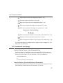
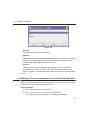
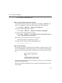
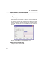
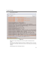
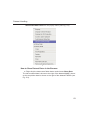
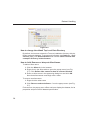
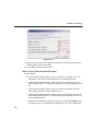
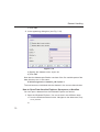
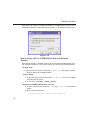
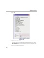
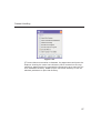
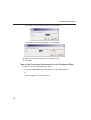
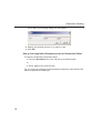
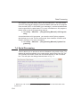
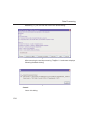
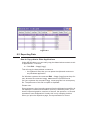
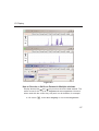
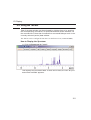
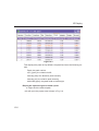
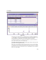
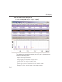
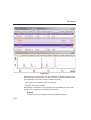
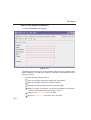
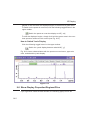
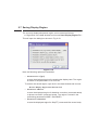
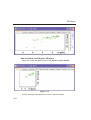
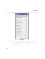
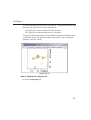
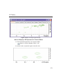
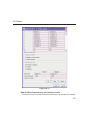
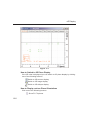
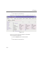
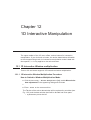
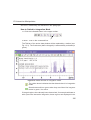
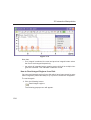
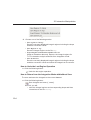
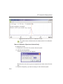
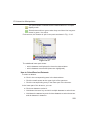
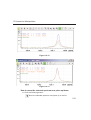
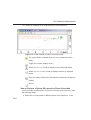
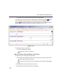
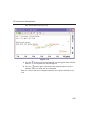
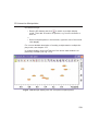
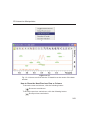
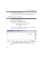
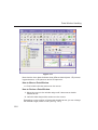
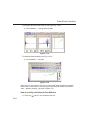
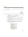
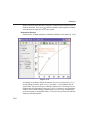
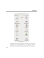
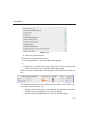
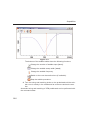
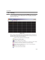
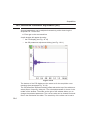
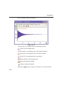
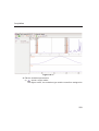
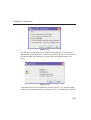
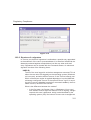
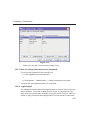
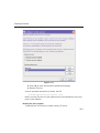
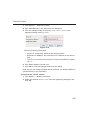
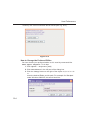
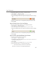
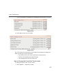
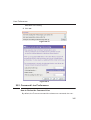
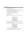
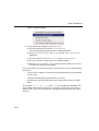
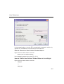
1D Display
INDEX
INDEX
DONE
Figure 9.6
As soon as you click a peak, it is selected and, by default, displayed in
red (see peak 1 in Fig. 9.6). Note that this peak remains selected, i.e. is
used by Enter and Delete, until a different peak is selected.
To extend the peak list, for example with Regions, Type and Index entries, right-click any part of the header bar.
To sort the peaks according to peak number, ppm value or intensity, click
the header of the respective entry.
Peaks are only available if peak picking has been done (command pp).
The peak list can be printed with print [Ctrl+p]. List items can be selected with the mouse, copied with Ctrl+c and pasted to other applications, e.g. a text editor.
133
1D Display
How to Display the Integral list
Click the Integrals tab [li, lipp, lippf]
INDEX
DONE
INDEX
Figure 9.7
This displays the integral list (upper part of Fig. 9.7). By default, this
shows the following items:
Object: the integral number
Integral [abs]: the absolute integral value
Integral [rel]: the relative integral value
Peaks: the number of peaks within the integral range
Range (F1) from: the left edge of the integral range
134
1D Display
Range (F1) to: the right edge of the integral range
Please note the difference between the following items:
INDEX
• selected integral: the entry that has been clicked last (Integral 3 in
Fig. 9.7).
If you right-click
INDEX
DONEan entry, it is selected and you can execute one of the commands from the popup menu (see Fig. 9.8)
The keys Enter and Delete work on the selected entry.
• active integral: the entry on which the cursor resides (Integral 1 in
Fig. 9.7). The active integral is also marked in the correlated spectrum by a black vertical line (see lower part of Fig. 9.7 and description below). When you move the cursor over the integral list, the
vertical line in the correlated spectrum moves along with it and
vice versa.
Note that the colours of the selected and active integral can be set in
the table properties (see below).
Display the spectral region around an integral
To display the spectral region around a particular integral:
Right-click the desired integral
135
1D Display
This will open the popup menu shown in Fig. 9.8.
INDEX
DONE
INDEX
Figure 9.8
Here you can choose from the following options:
Show spectrum In correlated spectrum
to open a new data window showing the full correlated spectrum
Expand spectrum In current window
to change the current data window to spectrum display, showing
the region around the selected integral
Expand spectrum In correlated window
to open a new data window showing the region around the selected integral (lower part of Fig. 9.7)
Note that clicking the marked entry in the right-click popup menu is
equivalent to pressing the Enter key.
Export/Import Entries of the Integral List
Entries of the integral list can easily be exported to Excel or any other
program as follows:
1. For multiple integrals:
136
1D Display
Select the desired entries while pressing the Ctrl or Shift key
2. Right-click an entry to open the popup menu (see Fig. 9.8)
INDEX
3. Click one of the following menu items:
INDEX
DONE
• Copy
Copy the selected integral(s) entry to the Clipboard. Equivalent
to clicking Edit Copy or hitting Ctrl+c. Copied integrals can
easily be pasted in any other application such as Excel.
• Export...
Export selected integrals. Check the box in the lower-left corner
to export the selected integrals only or uncheck it to export the
entire list. Then click Export.
Calibrate Integrals to Compare Spectra
Integrals from the current and other spectra can be calibrated with respect to a reference integral. To do that:
1. Right-click the reference integral and choose Define as reference
from the popup menu. This will determine the calibration constant.
2. Right-click any integral and choose Calibrate by reference
This will divide all integrals by the calibration constant, setting the
reference integral to 1.0.
Now you can read any other spectrum, and calibrate its integrals with
respect to the reference integral defined above. To do that:
1. Read the spectrum
2. Enter int to define the integral ranges (if this has not been done
yet)
3. Click the Integrals tab
4. Right-click any integral in the list and choose Calibrate by reference from the popup menu.
Note that the calibration constant is lost when TOPSPIN is restarted.
Display the integral list with peaks
The integral list in Fig. 9.7 shows only integrals. However, if peak picking has been done, the integral list also shows the peaks within each
integral range (see Fig. 9.9).
137
1D Display
INDEX
DONE
INDEX
Figure 9.9
Note that the integral entries can be collapsed, (hiding the peaks) or expanded (showing the peaks). As soon as one or more integrals entries
are expanded, two extra columns appear showing:
v(F1) [ppm]: the chemical shift of the peak
Intensity: the peak intensity
Depending on whether or not integrals are expanded, the right-click
popup menu contains the following extra items:
• Expand
Expand the current integral showing all peaks within it.
138
1D Display
• Expand all
Expand all integrals showing all peaks within them.
INDEX
• Collapse
all
Collapse all integrals hiding all peaks within them.
INDEX
DONE
In addition to the integral entry, an individual peak within an integral can
be activated (by placing the cursor on it) or selected (by clicking it). In
Fig. 9.9, peak 7 is selected and the correlated spectrum is displayed.
Peak 5 is active which is also shown by the vertical line in the correlated
spectrum.
Delete an Integral from the Integral List
To delete one integral:
Right-click the integral and choose Delete from the popup menu
To delete multiple integrals:
1. Select the integrals while pressing the Ctrl or Shift key
2. Right-click one of the integrals and choose Delete from the popup
menu
Note that these keys only work when the cursor focus is in the data window.
Table properties:
Various properties of the integral table can be configured. To do that:
1. Right-click an entry to open the popup menu (see Fig. 9.10).
2. Click Table properties...
3. In the appearing dialog box, with 3 tabs:
4. Columns
Allows you to select the columns to be displayed, set the column
• width and the number of fraction digits. Furthermore, you can
switch on/off scientific notation of values for each individual column.
• Colours
Allows you to set various colours of the table.
139
1D Display
• Spacings
Allows you to set various spacings of the table
INDEX
5.
DONE
INDEX
Figure 9.10
Shortcuts
Enter key: zoom into spectrum, i.e. show region around selected integral(s))
Delete key: delete the selected integral(s) from the integral list
140
1D Display
Ctrl+c: copy selected integrals to the Clipboard.
Ctrl+a: select all integrals.
INDEX
Home: select the first integral
INDEX
DONE
End: select the last integral
Shift+Home: select current and first integral and all in between
Shift+End: select current and last integral and all in between
Double-clicking an integral will show the peaks within the integral region if they exist. It they do not exist, it will zoom into spectrum showing the integral region.
Note that these keys only work when the cursor focus is in the data window.
141
1D Display
How to view Sample Information
Click the Sample tab [edsam]
DONE
INDEX
INDEX
Figure 9.11
This table can be used to fill out any sample information you want to store
with the dataset. The table can easily be modified or extended with the following functions:
To select an item: double-click it!
Save the sample information table with the dataset.
Save the sample information table as default.
Reload the original table discarding any changes
Add a new item to the table. You will be prompted for an identification name and the desired number of lines
Remove the selected item from the table
Move the selected item one place up in the table
142
1D Display
Move the selected item one place down in the table
How to OpenINDEX
the Jmol Molecule Structure Viewer
Click the Structure tab [jmol]:
INDEX
DONE
Figure 9.12
opens the Jmol molecule structure viewer. TOPSPIN 2.1 contains Jmol version 10. This has the following features:
• The viewer displays the structure file that resides in the expno of the
current dataset. If this does not exist, the structure file defined by the
acquisition parameter CHEMSTR is displayed. CHEMSTR can
define a full pathname or a filename. In the latter case, the file is
searched for in the directory defined in the User Preferences. To set
this directory, click Options Preferences, select Directory path
names, enter a directory and click OK. If no structure file is found,
you can open one by clicking File Open in the Molecule Viewer
• The following structure file types are supported: .xyz, .mol, .pdb,
.cml, .out, .mmlgp, .res, .cif, .gpr, .hin, .nwo.
143
1D Display
• Secondary structure elements of proteins (backbone, cartoons, ribbons, ...) can be displayed in selectable sizes and colors.
• Mouse button effects:
INDEX
Rotate a molecule aroundDONE
the x- and y-axis
by pressing the left mouse
INDEX
button, and moving the mouse left/right or up/down, respectively.
Rotate a molecule around the z-axis by pressing the middle mouse
button and moving the mouse left/right.
Zoom in or out a molecule by pressing the middle mouse button, and
moving the mouse up or down.
• RASmol command scripts are supported. To send a RASmol com-
mand to the currently displayed molecule enter:
jmol <RASmol command>
Here are some example:
jmol zoom 400
jmol ribbon 200
jmol color ribbon yellow
You may create TOPSPIN macros containing RASmol commands. Just
enter edmac on the TOPSPIN command line and insert the RASmol
commands in the appearing editor. Here is an example:
jmol load /mystructures/alphahelix.pdb # load a structure
jmol backbone 0.7 # display its backbone with 0.7 Angstrom size
jmol color backbone yellow # change backbone color
jmol background green # change background color
jmol zoom 200 # zoom structure
The available RASmol commands are described in the Jmol Help
menu.
• Multiple molecules (or multiple aspects of one molecule) can be displayed simultaneously. To do that just open multiple data sets or open
the same dataset in multiple data windows and click on the Structure
Tab in each window.
144
1D Display
How to Display the FID
Click the Fid tab [fid]
INDEX
INDEX
DONE
displays the raw data. If these do not exist, the text ’No raw data available’
appears. The following additional buttons appear at the right of the lower
toolbar:
Show FID in shuffled mode
Show FID in unshuffled mode
If you open a new dataset, the Spectrum tab is activated, no matter which
tab was selected before. If you enter any interactive mode, for example
phase correction mode, the Tab bar is replaced by a toolbar for that mode.
9.5 1D Display Options
How to Toggle between Hertz and ppm Axis Units
Click the following toggle button in the upper toolbar:
Toggle between Hz and ppm axis units [.hz]
How to Switch on/off the Spectrum Overview display
The spectrum overview shows the entire spectrum at the top of the data
window. It is useful when only a certain region of the spectrum is dis-
145
1D Display
played. In the overview, the displayed region is marked as a green area.
To switch on the spectrum overview, click the following toggle button in the
upper toolbar:
INDEX
INDEX
Switch the spectrumDONE
overview display
on/off [.ov]
To shift the displayed region, simply click-hold the green area in the overview spectrum and move the mouse (see Fig. 9.13).
How to Switch Y-axis Display
Click the following toggle button in the upper toolbar:
Switch the y-axis display between abs/rel/off [.y]
Fig. 9.13 shows a data window with the spectrum overview on, ppm axis
units, and absolute y-axis display.
Figure 9.13
9.6 Show Display Properties/Regions/Files
If you right-click inside the data window, the following popup menu will
146
1D Display
appear:
INDEX
INDEX
DONE
If you choose Display Properties..., a dialog box (see Fig. 9.14) will
appear.
147
1D Display
INDEX
DONE
INDEX
Figure 9.14
Here you can check or uncheck the spectrum components that you want to
be displayed in the data window.
Note that the Display Properties... dialog box can also be opened from
the View menu.
How to Superimpose the Cursor Information
To superimpose the cursor information on the spectrum:
148
1D Display
1. Right-click in the data window and choose Display Properties
[.dopt]
INDEXinformation in the appearing dialog box and click OK
2. Check Cursor
INDEX theDONE
How to Superimpose
Title on the Spectrum
1. Right-click in the data window and choose Display Properties...
[.dopt]
2. Check Title in the appearing dialog box and click OK
How to Superimpose the main Status Parameters on the Spectrum 1
1. Right-click in the data window and choose Display Properties...
[.dopt]
2. Check Status parameters in the appearing dialog box and click OK
How to Superimpose the Integral Trails/Labels on the Spectrum
1. Right-click in the data window and choose Display Properties...
[.dopt]
2. Check Integrals and, if desired, Integral labels in the appearing dialog box
3. Click OK
If no integrals appear, the integral regions have not been determined yet.
This can be done with the int command.
How to Superimpose Peak Labels on the Spectrum
1. Right-click in the data window and choose Display Properties...
[.dopt]
2. Check Peak labels in the appearing dialog box and click OK
If no peak labels appear, peak picking has not been done yet. This can be
done with the pp command.
1. These are the status parameters that also appear on the plot.
149
1D Display
How to Show Peak Annotations on the Spectrum
1. Right-click in the data window and choose Display Properties...
INDEX
[.dopt]
2. Check Peak labels and Peak
Annotations
in the appearing dialog
DONE
INDEX
box and click OK
Peak annotations appear, on peaks for which annotations have been defined, instead of regular peak labels showing chemical shift values. If no
peak labels or annotations appear, peak picking has not been done yet.
This can be done with the pp command.
How to Show Individual Data Points of the Spectrum
1. Right-click in the data window and choose Display Properties...
[.dopt]
2. Check Show data points in the appearing dialog box and click OK
3. Expand the spectral region where you want to see individual points.
How to Superimpose the Electronic Signature on the Spectrum
1. Right-click in the data window and choose Display Properties...
[.dopt]
2. Check Electronic Signature in the appearing dialog box and click
OK
The electronic signature, entered with esign, will appear below the title.
How to Display the Main Dataset Properties
Right-click inside the data window and choose File Properties
An information box as displayed in Fig. 9.15 will appear.
150
1D Display
INDEX
INDEX
DONE
Figure 9.15
Note that this is status information which cannot be changed.
How to Display a List of Files of a Dataset
Right-click inside the data window choose Files
Fig. 9.16 shows the file list when the Fid tab is active, i.e. when the raw
data are displayed. It is the contents of the expno directory.
151
1D Display
INDEX
DONE
INDEX
Figure 9.16
Fig. 9.17 shows the file list that appears when the Spectrum tab is active,
i.e. when the processed data are displayed. It is the contents of the procno
directory.
152
1D Display
INDEX
INDEX
DONE
Figure 9.17
The contents of any file in the list can be displayed as follows:
1. Select a filename (it will be highlighted)
2. Click Open
Note that this only makes sense for ascii files, e.g. acqu*, proc* or files
with the extension .txt.
Dataset files can also be displayed/opened with the command expl. This
opens the Windows Explorer, or under Linux, the Konqueror or Mozilla,
showing the contents of the procno directory.
153
9.7 Saving Display Region
The currently displayed spectral region can be stored as follows:
Right-click in the data window and choose Save Display Region To...
This will open the dialog box shown in Fig. 9.18.
Figure 9.18
Here the following options are available:
• Parameters F1/2 [dpl]
to save the displayed region for restoring the display later. The region
is stored in the parameters F1P and F2P.
To restore the saved region, right-click in the data window and choose:
Restore Display Region from Params F1/2
• Parameters ABSF1/2
to save the displayed region for baseline correction (command absf)
or phase correction (command apkf). The region is stored in the
processing parameters ABSF1 and ABSF2.
• Parameters STSR/STSI
to save the displayed region for Strip FT (commands like ft and trf).
The region is stored in the processing parameters STSR and STSI.
• Parameters NOISF1/2
to save the displayed region as the signal region for Signal to Noise
calculation (command sino). The region is stored in the processing
parameters SIGF1 and SIGF2.
• Parameters SIGF1/2
to save the displayed region as the noise region for Signal to Noise
calculation (command sino). The region is stored in the processing
parameters NOISF1 and NOISF2.
• A text file for use with other programs
to save the displayed region in a text file. This file can be viewed with
any editor or used by external programs.
9.8 Synchronize Visible Region of all Data Windows
The visible region of all data windows can be synchronizes as follows.
Zoom in or out one dataset while holding the Ctrl key
or
Zoom in or out one dataset and then enter the .sync command
1D Display
INDEX
DONE
156
INDEX
2D Display
Chapter 10
INDEX
INDEX
DONE
2D Display
10.1 The 2D Data Window
The 2D data window consists of a data field, a title bar, a Tab bar and buttons.
Fig. 10.1 shows a data window with a 2D spectrum.
157
2D Display
.
data
field
title bar
Tab bar
DONE
minimize
button
INDEX
maximize
button
close
button
INDEX
Figure 10.1
10.2 Changing the Display of a 2D spectrum
TOPSPIN offers various buttons to scale or shift a 2D spectrum both vertically and horizontally.
How to Change the Intensity Scaling (contour levels)
Click the button:
Change the intensity scaling (contour levels) [edlev]
or
Hit one of the keys:
• Alt+PageUp: Increase the intensity by a factor of 2.
• Alt+PageDown: Decrease the intensity by a factor of 2.
• Alt+Enter: Reset the intensity.
or
158
2D Display
Click one of the following buttons:
Increase the intensity (decrease the levels) by 2 [*2].
INDEX
Increase the intensity (decrease the levels) by 8 [*8].
INDEX
DONE
Decrease the intensity (increase the levels) by 2 [/2].
Decrease the intensity (increase the levels) by 8 [/8].
Reset the intensity to the last saved intensity (contour levels)
[.vr].
Alternatively, you can enter the corresponding commands as specified between square brackets [].
To manipulate all data windows, press the Ctrl key while clicking one of
the above buttons.
How to Smoothly Change the Vertical Scaling (contour levels)
To change levels, multiplying all levels with the same factor:
Click-hold the
button and move the mouse.
or
Turn the mouse wheel while the cursor is in the data window.
To change the level distance (increment), leaving the base level the same:
Click-hold the
button and move the mouse.
How to Display a Contour Levels Bar in the Data Window
1. Right-click in the data window and choose Display Properties...
[.dopt]
2. Check Contour Levels Bar in the appearing dialog box and click OK
(see Fig. 10.2).
159
2D Display
INDEX
DONE
INDEX
Figure 10.2
How to Switch on/off Square 2D layout
Right-click inside the data field and click Square Layout On/Off
Figure 10.3
The F2 scaling will be adjusted to reach a square display.
160
2D Display
How to Zoom a 2D spectrum in/out
Click one of the following buttons:
INDEX
Zoom in to the center (spectrum) or left edge (FID) of the disINDEX
DONE the horizontal scaling. [.zi]
played
region, increasing
Zoom out from the center (spectrum) or left edge (FID) of the displayed region, decreasing horizontal scaling) [.zo]
Perform an exact zoom via a dialog box [.zx].
Figure 10.4
a) Enter the coordinates of the desired region in the dialog box.
b) Click OK
Undo last zoom [.zl].
Show full spectral width in F2 [.f2r].
Show full spectral width in F1 [.f1r].
Show full spectrum [.all].
Retain horizontal and vertical scaling when modifying dataset or
changing to different dataset. Effects all data windows [.keep].
Alternatively, you can enter the corresponding commands as specified between square brackets [].
161
2D Display
How to Shift a Spectral Region in the F2 direction (left/right)
Click one of the following buttons:
INDEX
Shift to the left, half of the displayed region [.sl].
DONE
INDEX
Shift to the right, half of the displayed region [.sr].
or
Click-hold the button and move the mouse:
Smoothly shift in any direction.
Alternatively, you can enter the corresponding commands as specified between square brackets [].
How to Shift a Spectral Region in the F1 direction (up/down)
Click one of the following buttons:
Shift the spectrum up, half of the displayed region [.su].
Shift the spectrum down, half of the displayed region [.sd].
or
Click-hold the button and move the mouse:
Smoothly shift up/down and left/right.
Alternatively, you can enter the corresponding commands as specified between square brackets [].
10.3 Show Display Properties/Regions/Files
If you right-click inside the data window, the popup menu shown in Fig.
162
2D Display
10.5 will appear.
INDEX
INDEX
DONE
Figure 10.5
Here you can select various display properties, region setting and file properties. If you choose Display Properties..., a dialog box (see Fig. 10.6) will
appear.
163
2D Display
INDEX
DONE
INDEX
Figure 10.6
Here you can set various display options including parameter, integrals,
peaks, contours, projections and electronic signature. The number of displayed digits for the integral and peak labels can be set in the User Preferences (click Options Preferences Spectrum).
164
2D Display
10.4 Using the Tab bar
INDEXis a tabbed pane. This means its contents depends on
The 2D data window
the currently active tab in the Tab bar. The individual tabs are basically the
INDEX
DONE
same as for 1D display (see chapter 9.4). There are, however, some differences, which are discussed below.
How to Set Processing Parameters
Click the ProcPars tab [edp]
The 2D processing parameter editor contains a column for each of the
two dimensions F2 and F1 (see Fig. 10.7). Note that not all parameters
exist in both dimensions.
Figure 10.7
How to Set Acquisition Parameters
Click the AcquPars tab [eda]
The 2D acquisition parameter editor contains a column for each of the
two dimensions F2 and F1 (see Fig. 10.8). Note that not all parameters
165
2D Display
exist in both dimensions.
INDEX
DONE
INDEX
Figure 10.8
How to Display the Peak list
Click the Peaks tab
Figure 10.9
This displays list of peaks if these have been calculated (command pp).
166
2D Display
The list is basically the same as for 1D spectra. The only difference is that
there are two columns for the two dimensions:
INDEX
v(F2) [ppm]:
the chemical shift in the F2 direction
INDEX
DONE
v(F1) [ppm]:
the chemical
shift in the F1 direction
To specify or edit an annotation, click inside the Annotation field and enter
a character string. The peak annotations are shown in the correlated
spectrum (see Fig. 10.10)
Figure 10.10
How to Display the Integral list
Click the Integrals tab
167
2D Display
INDEX
DONE
INDEX
Figure 10.11
This displays list of integrals if these have been calculated (command
int). The list is basically the same as for 1D spectra. The only difference
is that, when peaks are shown, there are two columns for the chemical
shift:
v(F2) [ppm]: the chemical shift in the F2 direction
v(F1) [ppm]: the chemical shift in the F1 direction
Furthermore, a stored or exported 2D integral list can be imported as
follows:
1. Right-click an entry to open the popup menu
2. Click Import...
3. In the appearing dialog box, navigate to the directory where the list
resides and select the integral list.
As such you can import an integral list from a different dataset or a previously exported list from the current dataset. Note that integration
commands store the integral list in the processed data directory under
the name integrals.txt. Exported integrals are stored in the files
<name>.txt and <name>.reg, where <name> is the name specified
by the user.
168
2D Display
How to Display the FID
Click the Fid tab [fid]
INDEX
2D raw data consist of a series of FIDs which are displayed in a row. InINDEX
DONE
dividual FIDs
can be displayed
by zooming in. To do that, click
repeatedly. Now you can shift and zoom in/out the data to display different
FIDs (see Fig. 10.12)
.
Figure 10.12
10.5 2D Display Options
How to Switch between Hertz and ppm Axis Units in F2 and F1
Click the following multi-state button in the upper toolbar:
Switch between Hz and ppm axis units in F2 and F1 [.hz]
How to Switch on/off the Spectrum Overview display
Click the following toggle button in the upper toolbar:
Switch the spectrum overview display on/off [.ov]
With the spectrum overview on, the data window will, for example, look like
169
2D Display
this:
INDEX
DONE
INDEX
How to Switch on/off the Projection display
Click the following toggle button in the upper toolbar:
Switch the projection display on/off [.pr]
With the projections displayed, a 2D dataset looks like this:
170
2D Display
In this example, the F1 projection is selected as indicated by the filled blue
square whereas the F2 projection is not selected. A selected projection
can be rescaled
using the toolbar rescale buttons of function keys. If you
INDEX
right-click inside the projection area of the data window, the following popINDEX
DONE
up menu appears:
Clicking External Projection opens the a dialog box where you can specify or search for a 1D dataset and display this as a projection of the current
2D dataset.
Clicking Internal Projection calculates and displays the positive projection and displays it along with the 2D spectrum.
Clicking Baseline at Bottom or Baseline at Center allows you to put the
projection baseline at the respective positions.
Alternative ways to calculate/display projections are:
Right-click on a 1D dataset in the browser and choose:
Display As 2D Projection
or
Click Processing
Calculate projections [proj]
This will open the dialog box shown in Fig. 10.13.
171
2D Display
INDEX
DONE
INDEX
Figure 10.13
From here, you can calculate positive, negative, sum and disco projections and either show them with the 2D spectrum or display them
in separate data window as a 1D data. For more details on the corresponding commands (as shown in the header of the dialog box),
please refer to the Processing Reference Manual.
How to Switch on/off the Grid display
Click the following multi-state button in the upper toolbar:
Switch between ’no grid’, ’axis aligned grid’ and ’fixed grid’ [.gr]
Fig. 10.14 shows an example of axis aligned grid display.
172
2D Display
INDEX
INDEX
DONE
Figure 10.14 Axis aligned grid display
How to Display a 2D Spectrum in Contour Mode
Click the following button in the upper toolbar:
Switch to contour display mode [.co]
In contour mode, a spectral region looks like this:
173
2D Display
How to Set the 2D Contour Levels
Click the following button in the lower toolbar
Edit contour levels [edlev, .lv]
DONE
INDEX
INDEX
This will open the following dialog box shown in Fig. 10.15. Contour levels
can be entered manually or they can be calculated.
Manual setup
This allows you to create an arbitrary sequence of levels
1. Enter the level values in the fields 1, 2, ... at the top of the dialog
box.
2. Click Apply to update the display or OK to store the levels, update
the display and close the dialog box.
Calculation
This allows you to easily create a geometric or equidistant sequence of
levels.
1. Click one of the following items:
•
Multiply with increment
to create a geometric sequence of levels.
•
Add increment
to create a equidistant sequence of levels.
2. Enter the desired Base level, Level increment and Number of levels.
3. Click Fill to display and activate the sequence.
4. Click Apply to update the display or OK to store the levels, update
the display and close the dialog box.
The Contour level sign allows you to select positive levels, negative levels
or both.
174
2D Display
INDEX
INDEX
DONE
Figure 10.15
How to Store interactively set Contour Levels
To store contour levels that were set interactively, for example by clicking
175
2D Display
or pressing Alt+PageUp:
Click the following button in the lower toolbar:
Store contour levels [.ls]
DONE
INDEX
INDEX
The levels are stored in the file:
/<dir>/data/<user>/nmr/<name>/<expno>/pdata/<procno>/clevels
How to Display a 2D spectrum in Pseudo Color Mode
Click the following button in the upper toolbar:
Switch to image color display mode [.im]
In pseudo color mode, a spectral region looks like this:
Note that in pseudo color mode, the contours are superimposed, in black,
when you zoom in on a small region of the spectrum.
How to Display a 2D Spectrum in Oblique Mode
Click the following button in the upper toolbar
Switch to oblique display mode [.st]
In oblique mode, a spectral region looks like in Fig. 10.16.
176
Figure 10.16
In this mode you can manipulate the display in various ways. Just rightclick inside the data window and choose one of the options from the appearing popup menu (see Fig. 10.17)
2D Display
:
INDEX
DONE
INDEX
Figure 10.17
How to Rotate a 2D Spectrum in Oblique Mode
Click-hold one of the following button and move the mouse up/down:
Rotate around x-axis.
Rotate around y-axis.
How to Switch between Displaying Positive and Negative levels
Click the following multi-state button in the lower toolbar:
Switch between positive, negative and both contours [.lt].
178
nD Display
Chapter 11
INDEX
INDEX
DONE
nD Display
11.1 Display Planes of 3D Data
3D data can be displayed as 2D planes or as a 3D cube. By default, the
first F3-F1 plane is displayed (see Fig. 11.1) The plane orientation and
number is shown. The cube in the lower left corner graphically indicates
which plane is displayed. The full 2D display functionality is available (see
chapter 10).
179
nD Display
INDEX
DONE
INDEX
Figure 11.1
How to Switch to 2D Plane Display
If the 3D cube is displayed you can switch to 2D plane display by clicking
one of the following buttons:
Switch to 2D contour display.
Switch to 2D image display.
Switch to 2D oblique display.
How to Display various Plane Orientations
Click one of the following buttons:
Show F1-F2 planes.
180
nD Display
Show F2-F3 planes.
Show
F3-F1 planes.
INDEX
INDEX
DONE
How to Display various Plane Positions (numbers)
Click one of the following buttons:
Show the next plane.
Show the previous plane.
Scan planes smoothly.
Enter the exact plane number. This will open the dialog shown in
Fig. 11.2. Here, you can specify the desired plane number as
well as switch to a different plane orientation.
Figure 11.2
181
nD Display
11.2 3D Cube Display Mode
How to Display the 3D Cube
Click the following button: DONE
INDEX
INDEX
Show 3d cube (see Fig. 11.3).
Figure 11.3
How to Rotate the 3D Cube
Click-hold one the following buttons and move the mouse up/down:
Rotate cube around x-axis.
Rotate cube around y-axis.
Rotate cube around z-axis.
182
nD Display
How to Scale Up/Down the 3D Cube
1. Right-click inside the data window.
2. Choose INDEX
Larger or Smaller from the popup menu (see Fig. 11.4).
INDEX
DONE
How to Reset the Cube Size and Orientation
Click the following button:
Reset to default size and orientation.
How to Switch Depth Cueing on/off
1. Right-click inside the data window
2. Choose Depth Cueing On/off (see Fig. 11.4)
Depth cueing makes data points which are closer to the viewer appear
brighter and those that are further away appear dimmer. This increases
the depth effect of the 3D image.
Figure 11.4
How to Display a Cube Front or Side view
Click one the following buttons:
Show F1-F2 plane.
Show F2-F3 plane.
Show F3-F1 plane.
11.3 nD parameter display
TOPSPIN 2.1 and newer support parameter display of up to 8D data. To
show processing parameters:
click the ProcPars tab of the data window
183
nD Display
or
enter edp on the command line
INDEX
Parameters of each direction are shown in a separate column. Fig. 11.5
DONE
INDEX
Figure 11.5
shows the processing parameter display of a 3D dataset.
To show acquisition parameters:
click the AcquPars tab of the data window
or
enter eda on the command line
184
nD Display
Parameters of each direction are shown in a separate column. Fig. 11.5
INDEX
INDEX
DONE
Figure 11.6
shows the acquisition parameter display of a 3D dataset.
11.4 nD Fid Display
nD raw data can be displayed as a series of 1D FIDs. To do that:
click the FID tab of the data window
or
enter fid on the command line
185
11.5 nD Peak and Integral Display
TOPSPIN 2.1 and newer support peak and integral display of up to 8D data.
To show the nD peak list:
click the Peaks tab of the data window
or
enter peaks on the command line
Fig. 11.7 shows the peak list of a 3D dataset.
Figure 11.7
The chemical shift in each of the three dimensions is shown in a separate
column.
nD Display
To show the nD integral list:
INDEX
click the Integrals tab of the data window
or
INDEX
DONE
enter ints on the command line
Fig. 11.7 shows the integral list of a 3D dataset.
Figure 11.8
The chemical shift in each of the three dimensions is shown in a separate
column.
Peaks and integrals only appear if they have been calculated (commands
pp and int, respectively).
187
nD Display
INDEX
DONE
188
INDEX
Chapter 12
1D Interactive Manipulation
The upper toolbar of the 1D menu offers various buttons for interactive
manipulation. If you click such a button, the active data window will switch
to the corresponding mode. An interactive manipulation mode is data window specific, i.e. it only applies to the active window.
12.1 1D Interactive Window multiplication
TOPSPIN 2.0 and newer supports 1D interactive window multiplication.
12.1.1 1D Interactive Window Multiplication Procedure
How to Switch to Window Multiplication Mode
Click the Processing Window Multiplication [wm], enable Manual window adjustment in the appearing dialog and click OK.
or
Enter .winf on the command line.
The Tab bar of the active data window will be replaced by a toolbar (see
Fig. 12.2) and the data window itself will be divided into three parts:
• a parameter part at the left
1D Interactive Manipulation
• a spectrum part at the upper right
• a FID part at the lower right.
INDEX
DONE
INDEX
Figure 12.1
Show both spectrum and FID.
Show FID only.
Show spectrum only.
Switch cursor information on/off (toggle)
Save windows settings to source 2D dataset1 and return.
1. 2D data from which current 1D dataset was extracted, e.g. with rser.
190
1D Interactive Manipulation
Save window settings and return
Return
without save.
INDEX
INDEX
DONE
You can perform
interactive
window manipulation as follow:
1. Select the window function (parameter WDW)
2. Set the corresponding parameter(s), e.g.
• LB for exponential
• LB and GB for Gaussian
• SSB for sine bell and squared sine
The displayed spectrum and/or FID will be automatically adjusted
as you change the window function and parameters.
3. Click
to store the window settings and return.
Now you can perform further processing steps like Fourier transform,
phase correction etc.
12.2 1D Interactive Phase Correction
Manually acquired spectra can be phased corrected automatically, with
commands like apk or apks or, interactively, in phase correction mode.
12.2.1 1D Interactive Phase Correction Procedure
How to Switch to Phase Correction Mode
Click the indicated button in the upper toolbar:
or enter .ph on the command line.
The Tab bar of the active data window will be replaced by a toolbar (see
Fig. 12.2)
191
1D Interactive Manipulation
INDEX
DONE
INDEX
Figure 12.2 Data window in phase correction mode
The yellow button indicates that you are in phase correction mode.
Some buttons will turn green when they are clicked. As long as a
button is green, it is active.
How to Perform a Typical 1D Interactive Phase Correction
For a typical 1D phase correction, take the following steps:
1. Click-hold the button
and move the mouse until the until the reference peak is exactly in absorption mode.
2. Click-hold the button
and move the mouse until the entire spectrum is exactly in absorption mode.
3. Click the button
return.
to save and execute the phase correction and
12.2.2 1D Interactive Phase Correction Details
How to Set the Phase Pivot Point
By default, the phase pivot point is set to the biggest magnitude intensity
of the displayed region of the spectrum. To change the pivot point:
1. Right-click on the desired pivot point position
2. Choose Set pivot point from the popup menu (see Fig. 12.2)
192
1D Interactive Manipulation
How to Perform Default Zero Order Phase Correction
1. Right-click in the data window
2. Choose INDEX
Calculate ph0 in the popup menu (see Fig. 12.2)
INDEX
DONE
The spectrum
will automatically
be corrected according to the calculated
value.
How to Perform Interactive Zero Order Phase Correction
1. Click-hold the following button (button turns green):
Zero order phase correction (parameter PHC0).
2. Move the mouse until the reference peak is exactly in absorption
mode.
3. Release the mouse (button turns grey).
How to Perform Interactive First Order Phase Correction
1. Click-hold the following button (button turns green):
First order phase correction (parameter PHC1).
2. Move the mouse until the entire spectrum is exactly in absorption
mode.
3. Release the mouse (button turns grey).
How to Perform 90, -90 or 180° Zero Order Phase Correction
Click one of the following buttons:
Perform 90 zero order phase correction [.ph90].
Perform -90° zero order phase correction [.phm90].
Perform 180° zero order phase correction [.ph180].
How to Reset the Phase to the Original Values
Click the following button:
Reset zero and first order phase values [.phr].
193
1D Interactive Manipulation
How to Change the Mouse Sensitivity
Click one of the following buttons:
INDEX
Increase (double) the mouse sensitivity [.inc].
DONE
INDEX
Decrease (halve) the mouse sensitivity [.dec].
Reset the mouse sensitivity.
How to Return from Phase Correction Mode with/without Save
To return while saving the phase correction to the current dataset:
Click the following button:
Save, execute and return [.sret].
This will perform the following tasks:
• Execute phase correction (command pk).
• Save the current phase correction values.
• Leave the phase correction mode.
To return without save:
Click the following button:
Return, discarding any changes [.ret].
To return while saving the phase correction to the source 2D dataset:
Click the following button:
Save to 2D [.s2d].
This is only applicable on rows or columns extracted from 2D data.
The phase values will be saved to the 2D dataset from which the current 1D dataset was extracted.
12.3 1D Interactive Integration
Integration of 1D data can be done automatically, with the commands abs
194
1D Interactive Manipulation
and li or, interactively, as described in this paragraph.
How to Switch
to Integration Mode
INDEX
Click the indicated button in the upper toolbar:
INDEX
DONE
or enter .int on the command line.
The Tab bar of the active data window will be replaced by a toolbar (see
Fig. 12.3). The first button (define integrals) is automatically activated (is
green).
Figure 12.3 Data window in integration mode
The yellow button indicates that the data window is in integration
mode.
Some buttons will turn green when they are clicked. As long as a
button is green, it is active.
If integral regions have already been determined, for example with abs or
with a previous interactive integration, these regions are displayed in the
195
1D Interactive Manipulation
data window, along with the integral values. You can remove them,
change them or add to them, as described below.
How to Define Integral Regions
DONE
To define integral regions interactively:
INDEX
INDEX
1. Click the following button (button turns green):
Define integral region interactively.
Note that the define integrals button is automatically activated on entering the integrals mode.
2. Put the red cursor line at one edge of a peak or multiplet.
3. Left-click-hold and drag the cursor line to the other edge of the peak
or multiplet.
4. Do step 2 and 3 for all regions to be defined.
5. Click the green button to leave the "define region" mode (button turns
grey).
To define integral regions via a dialog box:
1. Click the following button:
Define region via dialog.
2. In the appearing dialog box:
Enter the exact values for the region limits.
3. Click OK to define the selected region.
196
1D Interactive Manipulation
How to Select/Deselect Integral Regions
To select/deselect all displayed integral regions:
INDEX
Click the button:
INDEX
button
DONE
To select a single integral region:
1. Right-click in the integral region.
2. Choose Select/Deselect from the popup menu.
To select the next integral region:
Click the
button
To select the previous integral region:
Click the:
button.
To select multiple integral regions:
1. Click the button:
button to select all integrals
2. Deselect the integral that are not to be selected.
Selected integral regions are indicated by a color filled integral label. In the
Fig. 12.4, the five left most regions are selected, the region around 6 ppm
is currently being deselected.
197
1D Interactive Manipulation
INDEX
DONE
INDEX
Figure 12.4
Note that:
• If no integral is selected, the next and previous integral button select
the first or last integral respectively.
• the select all integrals button remains green while all or multiple integrals are selected. This indicated a selection mode.
How to Read Integral Regions from Disk
You can read integrals regions from disk which have been stored by automatic integration (command abs) or by a previous interactive integration.
To read integrals:
1. Click the following button:
Read integral regions.
The following popup menu will appear:
198
1D Interactive Manipulation
INDEX
INDEX
DONE
Figure 12.5
2. From the popup menu, choose one of the following entries:
• Read ’intrng’
to read the last saved integral regions and apply the saved slope
and bias correction values.
• Read ’intrng’ no slope & bias corr.
to read the last saved integral regions but do not apply the saved
slope and bias correction values.
• Read ’intrng’ use last slope & bias
to read the last saved integral regions applying the last slope and
bias correction values.
• Read ’intrng’ from Relaxation Experiment
to read the last stored integral regions of the T1/T2 relaxation
experiment.
• Edit ’intrng’
to edit the file (intrng) that contains the integral regions and
slope and bias correction values. Changes in this file are automatically shown on the screen.
How to Perform Interactive Bias and Slope Correction
To perform interactive bias correction:
1. Select the integral(s) that you want to correct (right-click in the
region).
If no integral is selected, bias correction will work on all integrals.
2. Click-hold the following button (it turns green) and move the mouse,
Integral bias correction.
199
1D Interactive Manipulation
until the integral bias is correct.
3. Release the mouse (button turns grey).
To perform interactive slope correction:
INDEX
INDEX(right-click in the
1. Select the integral(s) thatDONE
you want to correct
region).
If no integral is selected, slope correction will work on all integrals.
2. Click-hold the following button (it turns green) and move the mouse,
Integral slope correction.
until the integral slope is correct.
3. Release the mouse (button turns grey).
How to Set the Limit for Bias Determination
Click the following button:
Limit for bias determination.
How to Change the Mouse Sensitivity
Click one of the following buttons:
Increase (double) the mouse sensitivity [.inc].
Decrease (halve) the mouse sensitivity [.dec].
Reset the mouse sensitivity.
How to Calibrate/Normalize Integrals
Calibrating integrals means setting the value of a reference integral and
adjusting all other integrals accordingly. To do that:
1. Right-click in the reference integral region.
2. Choose Calibrate from the popup menu (see Fig. 12.6).
3. Enter the desired value for the reference integral and click OK
Normalizing integrals means setting the sum of all integrals and adjusting
individual integral values accordingly. To do that:
200
1D Interactive Manipulation
1. Right-click in the reference integral region.
2. Choose Normalize from the popup menu (see Fig. 12.6).
INDEX
3. Enter the desired sum of all integrals and click OK
INDEX
DONE
Figure 12.6
Calibrating and normalizing only effects the current dataset. To scale integrals with respect to a reference dataset, choose lastscal from the
right/click popup menu (see below).
How to Scale Integrals with respect to Different Spectra
Integrals can be scaled with respect to the last spectrum that was integrated interactively. To do that:
1. Right-click in the reference integral region.
2. Choose Lastscal from the popup menu (see Fig. 12.6).
As such, you can compare integrals of different spectra. Note that this only
make sense for spectra which have been acquired under the same experimental conditions. The scaling factor is stored in the file:
<tshome>/prog/curdir/<user>/intscale
How to Delete Integral Regions from the Display
To delete the selected integral regions from the display:
Click the following button:
Delete selected integral regions from the display.
To delete a single integral region from the display:
1. Right-click in the integral region.
2. Choose Delete from the popup menu (see Fig. 12.6)
201
1D Interactive Manipulation
To delete all integral regions from the display:
Click the following buttons:
Select all integral regions.
DONE
INDEX
INDEX
Delete selected integral regions from the display.
Note that regions are only deleted from the screen. Regions which are
saved on disk (in the intrng file) are not affected.
How to Scale Selected Integrals
Integral scaling only manipulates selected integrals. However, if no integrals are selected, it works on all integrals.
Click one of the following buttons:
Scale up selected integrals by a factor of 2.
Scale down selected integrals by a factor of 2.
Scale selected integrals up/down smoothly.
To scale up/down integrals by a factor entered via a dialog:
1. Click the following button:
Scale integrals via a dialog.
2. Enter a scaling factor, e.g. 2.5. in the appearing dialog.
3. Click OK to apply this factor.
To scale all integrals to the same height:
Click the following button:
202
1D Interactive Manipulation
Scale/unscale all integrals to the same height.
The individual
scaling factor for each region is displayed above the inINDEX
tegral. Clicking this button again rescales all integrals to their original
DONE
height. INDEX
How to Move the Integral Trails Up/Down
To move the integrals (selected and unselected) up or down:
Click one of the following buttons:
The left edge of the selected integral is put just above the baseline. If no integral is selected, the lowest integral is used.
The right edge of the selected integral is put at 3/4 of the window
height. If no integral is selected, the highest integral is used.
Shift all integral trails up/down smoothly.
How to Cut Integral Regions
1. Click the following button (button turns green):
Cut integral region.
2. Move the red cursor line into an integral region to the position where
it must be cut and click the left mouse button.
3. Do step 2 for each integral region that must be cut.
4. Click the (green) button to leave the cut integral mode (button turns
grey).
In case of overlapping integrals, you must select the integral to be cut before you actually cut it.
How to Save Integral Regions
1. Click the following button:
Save integral regions.
The following popup menu will appear:
203
1D Interactive Manipulation
es
INDEX
DONE
INDEX
Figure 12.7
2. Choose one of the following entries:
• Save regions to ’intrng’
Save the currently displayed integral regions including the slope
and bias correction values.
• Save Regions to ’reg’
Save the integral regions to the file reg.
• Export Regions To Relaxation Module and .sret
Used on relaxation data only. Exports the integral regions for
T1/T2 relaxation analysis and exits from integration mode.
• Save & show list
Save the currently displayed integral regions including the slope
and bias correction values and show the integrals on the screen.
How to Undo the Last Region Operation
Click the following button:
Undo the last region operation.
How to Return from the Integration Mode with/without Save
To return and save the integrals to the current dataset:
Click the following button:
Save integrals and return [.sret].
As such, you will:
• save the integral regions and corresponding slope and bias
corrections to the file intrng.
204
1D Interactive Manipulation
• save the integral regions, slope and bias corrections and integral values to the file integrals.txt. This file is displayed
when
you click the Integrals Tab.
INDEX
• leave the integration mode.
INDEX
DONE
To return without save:
Click the following button:
Return, discarding any changes [.ret].
12.4 1D Interactive Calibration
A 1D spectrum can be calibrated (referenced), automatically, with the command sref or, interactively, as described below.
How to Switch to Calibration Mode
Click the indicated button in the upper toolbar
or enter .cal on the command line. The Tab bar of the active data window
will be replaced by a toolbar.
205
1D Interactive Manipulation
INDEX
DONE
INDEX
Figure 12.8 Data window in calibration mode
The yellow button indicates that the data window is in calibration
mode.
How to Calibrate a Spectrum Interactively
In calibration mode:
1. Position the red cursor line at the reference peak.
2. Left-click at that position.
The following dialog box will appear:
Note that the units (Hz or ppm) correspond to the axis units of the display.
3. Enter the frequency you want to assign to the reference peak.
206
1D Interactive Manipulation
4. Click OK
The spectrum will be calibrated and re-displayed. TOPSPIN will automatiINDEX mode.
cally leave calibration
INDEX
DONE
12.5 1D Multiple Display
The multiple display mode allows you to display multiple superimposed
spectra.The spectra will be ppm aligned or Hz aligned, according to the
selected axis unit. Each spectrum can be individually shifted and scaled
allowing exact alignment of corresponding peaks in different spectra. The
number of superimposed spectra is unlimited.
Although multiple display is normally used for spectra with matching nuclei,
it allows you to superimposed spectra with non-matching nuclei. You will
get a warning that the nuclei do not match. Just just click OK to continue.
How Switch to Multiple Display Mode and Read Multiple Spectra
One way to superimpose data in multiple display is to read one dataset,
switch to multiple display mode and add other datasets:
1. Read a 1D dataset.
2. Click the
mand line.
button in the upper toolbar or type .md on the com-
The data window will switch to multiple display mode.
3. Add a dataset as follows:
Left-click-hold the dataset in the browser and drag it into the data
window.
or
Right-click the dataset in the browser and choose Display from the
popup menu.
or
Enter re and specify the additional dataset in the appearing dialog
box.
Another way to superimpose data in multiple display is to read multiple
207
1D Interactive Manipulation
datasets simultaneously:
1. In the browser:
INDEX
Hold down the Ctrl key and click multiple datasets to select them.
or
DONE
INDEX
Hold down the Shift key and click two datasets to select these
two and all datasets in between.
2. Right-click any of the selected data:
Choose Display from the popup menu.
This will show the data in the active data window if that is in multiple display mode or, otherwise, show the data in a new window.
or
Choose Display in new window from the popup menu.
This will show the data in a new window.
In multiple display mode, the Tab bar of the active data window is replaced by a toolbar. Fig. 12.9 shows three comparable 1D spectra and
the sum of all three.
Figure 12.9 Data window in multiple display mode
208
1D Interactive Manipulation
The yellow button indicates that the data window is in multiple
display mode.
INDEX
Some
buttons will turn green when they are clicked. As long as a
button
is green, it DONE
is active.
INDEX
Furthermore, the browser is split in two parts as shown in Fig. 12.10.
Figure 12.10
The additional lower part shows:
• which datasets are displayed in the active data window.
• which datasets are selected (these are highlighted).
How to Select/Deselect Datasets
To select a dataset:
Click in the corresponding area in the data window.
or Click the small square at the upper right of the spectrum.
or Click the corresponding entry in the lower part of the browser.
In the lower part of the browser, you can:
Click one dataset to select it.
or Hold down the Ctrl key and click multiple datasets to select them.
or Hold down the Shift key and click two datasets to select these two
and all datasets in between.
209
1D Interactive Manipulation
When you select a dataset, the corresponding small square is filled (see
Fig. 12.9) and its entry in the lower part of the browser is highlighted (see
Fig. 12.10).
INDEX
Note that:
DONE
INDEX
• no spectrum selected = all spectra selected
• scale/shift buttons of the data window toolbar only work on
selected spectra
To deselect a dataset:
Select a different dataset.
To deselect all datasets:
Click the following button:
Deselect all datasets.
How to Remove a Dataset from Multiple Display
1. Select the dataset(s) you want to remove.
2. Click the following button:
Remove selected data from the screen.
Note that the data on disk are not affected. Furthermore, the first spectrum
cannot be removed from the screen.
How to Display the Sum or Difference Spectra
Click one of the following button (button turns green):
Show the difference between the first and the sum of the other
datasets.
Show the sum of all datasets in the multiple display window.
How to Save the Sum or Difference Spectra
1. Click the following button:
Save the displayed sum or difference spectrum.
2. In the appearing dialog box, specify the destination procno.
210
1D Interactive Manipulation
How to Display the Next/Previous Name/Expno
To compare a series of spectra you can interactively increment or decreINDEX
ment the dataset
name or expno. A dataset name is incremented according to the ICON-NMR naming convention of increasing extensions, e.g.
INDEX
DONE
name.001, name.002 etc.
Click one of the following button (button turns green):
Show the previous name/expno/procno of the last dataset
Show the previous name/expno/procno of the last dataset
Set the increment options. Clicking this button will open the following dialog:
Figure 12.11
Here you can choose to increment the procno, expno or name, set the
expno increment and switch individual scaling on/off.
How to Toggle between Superimposed and Stacked Display
Click the following button:
Toggle between superimposed and stacked display.
211
1D Interactive Manipulation
How to Shift and Scale Individual Spectra
To compare the intensity and chemical shift of corresponding peaks, you
can shift and scale individual spectra. To doINDEX
this:
1. Display the spectra in multiple
mode as described above.
DONEdisplay INDEX
2. Expand the spectra to display the desired region or peak.
3. Select one of the spectra (e.g. by clicking it in the lower part of the
browser).
4. Click-hold the
ties.
button and move the mouse to align the intensi-
5. Click-hold the
tions.
button and move the mouse to align the peak posi-
The alignment can be facilitated by showing the difference spectrum (
button) and minimize that. Note that you can also scale the selected spectra up/down with the buttons
and
. The
move the selected spectra vertically. Clicking the
button allows you to
button resets individ-
ual scaling and shifting.
The performed scaling and shifting are displayed in the data window (see
Fig. 12.12 and 12.13).
212
1D Interactive Manipulation
INDEX
INDEX
DONE
Figure 12.12
Figure 12.13
How to move the selected spectrum one place up/down
Click the following button:
Move the selected spectrum one place up in the list.
213
1D Interactive Manipulation
Click the following button:
Move the selected spectrum one place down in the list.
INDEX
Note that the first spectrum and calculated spectra (sum of difference)
INDEX
cannot be moved up/down. DONE
How to Switch on/off the Display of Datapaths and Scaling Factors
Click the following button:
Switch on/off display of datapaths and scaling factors.
How to Return from Multiple Display mode
Click the following button:
Return from multiple display mode [.ret].
How to Set the Colors of the 1st, 2nd, .. Dataset
The colors of the different datasets in the multiple display mode can be set
in the User preferences dialog box. To set, for example, the color of the second spectrum:
Click Options Preferences and click the Change button for the item
Color of 2nd 1D spectrum.
TOPSPIN 2.0 and newer allows you to set 8 different colors for different
spectra in multiple display.
12.6 1D Interactive Baseline Correction
Baseline correction can be performed with commands like abs or absd or,
interactively, as described below.
How to Switch to Baseline Correction Mode
Click the indicated button in the upper toolbar:
214
1D Interactive Manipulation
INDEX
INDEX
DONE
or enter .basl on the command line.
The Tab bar of the active data window will be replaced by a toolbar (see
Fig. 12.14).
Figure 12.14 Data window in baseline correction mode
The yellow button indicates that the data window is in baseline
correction mode.
Some buttons will turn green when they are clicked. As long as a
button is green, it is active.
How to Perform Polynomial Baseline Correction
1. Click the following button (button turns green):
Perform polynomial baseline correction.
In the data window, a red horizontal line will appear as well as the
equation that describes the polynomial function:
215
1D Interactive Manipulation
2. Click-hold button A and move the mouse until the red line coincides
with the first point of the spectrum.
3. Repeat step 2 with the buttons B, C, DINDEX
and E until the red line coincides with the entire baseline of the spectrum.
DONE
INDEX
How to Perform Sine Baseline Correction
1. Click the following button (button turns green):
Perform sine baseline correction.
A red horizontal line will appear as well as the equation describing the
sine function:
2. Click-hold button A and move the mouse until the red line coincides
with the first point of the spectrum.
3. Repeat step 2 with the buttons B, C and D until the red line coincides
with the entire baseline of the spectrum.
How to Perform Exponential Baseline Correction
1. Click the following button (button turns green):
Perform exponential baseline correction.
A red horizontal line will appear as well as the equation describing the
exponential function:
2. Click-hold button A and move the mouse until the red line coincides
with the first point of the spectrum.
3. Repeat step 2 with the buttons B and C until the red line coincides
with the entire baseline of the spectrum.
How to Preview the Baseline Corrected Spectrum
Before actually performing the baseline correction, you can preview the
result by displaying the difference between the uncorrected spectrum and
the red correction line.
216
1D Interactive Manipulation
To do that:
1. Click the following button (button turns green):
INDEX
Preview corrected spectrum (show difference).
INDEX
DONE
The corrected
spectrum
will be displayed in red.
2. If the baseline is correct, click the
button to save the correction. If
further correction is needed, click the
button to show the original
spectrum and the red correction line.
How to Reset the Baseline Correction Line
1. Click the following button:
Reset the red correction line to zero.
If the difference spectrum is displayed (the
button is active), clicking the reset button will restore the original spectrum.
How to Change the Mouse Sensitivity
Click one of the following buttons:
Increase (double) the Mouse Sensitivity [.inc].
Decrease (halve) the Mouse Sensitivity [.dec].
Reset the Mouse Sensitivity.
How to Save the Baseline Correction and/or Return
To return while saving the baseline correction:
Click the following button:
Save baseline correction and Return [.sret]
This will perform the following tasks:
• Execute the baseline correction [bcm].
• Save the baseline correction values A, B, C, D and E.
• Leave the baseline correction mode.
To return while discarding any changes:
217
1D Interactive Manipulation
Click the following button:
Return, Discarding any changes [.ret].
INDEX
How to Perform Cubic Spline
BaselineINDEX
correction
DONE
Click the following button:
Define points for cubic spline baseline correction.
The toolbar of the data window will change as shown in Fig. 12.15.
Figure 12.15 Data window in spline baseline correction mode
The cursor line in the data window turns red. If a list of baseline points already exists, you are prompted to overwrite or append to these points. If
you choose Append, the labels of the existing points are displayed on the
screen. If you choose Overwrite, no labels are displayed. Nevertheless,
the existing points are only overwritten when you define and save new
points.
To define new baseline points:
1. Move the cursor line to a baseline point and left-click at that position.
2. Do this for at least five baseline points.
Fig. 12.15 shows a spectrum with five defined baseline points. Note that
here the points have been chosen at the right part of the spectrum for dis-
218
1D Interactive Manipulation
play reasons only.
How to Delete
Spline Baseline Points from the screen
INDEX
To delete one baseline point:
INDEX
DONE
1. Right-click the baseline point position in the data window.
2. Choose Delete Current from the popup menu (see Fig. 12.16).
Figure 12.16
To delete all baseline points:
1. Right-click any position in the data window.
2. Choose Delete All from the popup menu (see Fig. 12.16).
How to Return from Cubic Spline Baseline mode with/without
Save
To return while saving the baseline points:
Click the following button:
Save baseline points and Return [.retsab].
To return while discarding any changes:
Click the following button:
Return, Discarding any changes [.ret].
Alternatively, you can right-click in the data window and choose Save &
Quit or Quit, respectively.
219
1D Interactive Manipulation
12.7 1D Interactive Peak Picking
INDEX
Peak picking can be performed, automatically,
with the commands pps or,
interactively, in the peak picking mode.
DONE
INDEX
How to Switch to Peak Picking Mode
Click the indicated button in the upper toolbar:
or enter .pp on the command line.
The Tab bar of the active data window will be replaced by a toolbar (see
Fig. 12.17).
Figure 12.17 Data window in peak picking mode
The yellow button indicates that you are in peak picking mode.
Some buttons will turn green when they are clicked. As long as a
button is green, it is active.
220
1D Interactive Manipulation
Note that the
button is automatically activated, i.e. you are in Define
peak picking range mode
INDEX
How to Define New Peak Picking Ranges
INDEX
DONE corner of a peak picking range.
1. Put the cursor
at the upper-left
2. Left-click-hold and drag the mouse to the lower-right corner of the
range.
The peak picking range will be marked green. The minimum and maximum intensity are set and the peaks in the range are picked and displayed.
3. Repeat step 1 and 2 for each peak picking range to be defined.
4. Click the green button to leave the "Define peak picking range"
mode.
Note that the parameters MI and MAXI are set to the lowest minimum and
the highest maximum intensity, respectively, of all ranges.
How to Change Peak Picking Ranges
1. Click the following button (button turns green):
Change peak picking ranges.
2. Put the cursor on one of the edges of the peak picking range.
The cursor turns into a double-headed arrow.
3. Left-click-hold and drag the peak range edge to its new position.
4. Optionally: repeat step 2 and 3 for the other edge and for other peak
ranges.
5. Click the green button to leave the "Change peak picking range"
mode.
How to Pick Peaks in Peak Picking Ranges only
Peaks in a peak range are automatically picked when the range is defined.If peaks have been deleted from a rang, they can be picked again as
follows:
1. Right-click in the data field.
2. Choose Pick Peaks On Ranges from the popup menu.
221
1D Interactive Manipulation
Alternatively, you can enter ppl on the command line. This command can
be entered in Interactive peak picking mode or in the normal display mode.
INDEX
How to Delete all Peak Picking Ranges
DONE
INDEX
Click the
button in the data window toolbar.
or
Right-click in the data field and click Delete All Ranges in the popup
menu.
How to Define Peaks Manually
1. Click the following button (button turns green):
Define peaks manually.
A red vertical line will appear in the data window.
2. Put the red cursor line at the desired peak and click the left mouse
button.
The peak label will appear at the top of the data window.
3. Repeat step 2 for each peak to be defined.
4. Click the green button to leave the "Define peaks" mode.
How to Pick Peaks Semi-Automatically
1. Click the following button (button turns green):
Define peaks semi-automatically.
2. Move the cursor into the data window.
3. Put the cursor line near the desired peak.
4. Left-click to pick forward
or
Right-click to pick backward (see Fig. 12.18).
A red cursor line will appear at the nearest peak whose intensity is between MI and MAXI.
5. Right-click to add the selected peak to the peak list (see Fig. 12.18).
222
1D Interactive Manipulation
INDEX
INDEX
DONE
Figure
12.18
The peak label will appear at the top of the data window.
6. Click the green button to leave the "define peaks semi-automatically"
mode.
How to Delete Peaks from the Peak List
To delete a specific peak:
1. Right-click on a defined peak.
2. Choose Delete peak under cursor from the popup menu (see Fig.
12.19).
99
Figure 12.19
To delete all peaks:
Click the
button in the data window toolbar.
or
Right-click in the data field and click Delete All Peaks in the popup
menu.
223
1D Interactive Manipulation
How to Return from Peak Picking Mode with/without Save
To return while saving the peak list and peak ranges:
Click the following button:
DONE
INDEX
INDEX
Save the Peak Region and Peak List and Return [.sret].
This will:
• Save the peak list to the file peak.xml and the peak ranges to
the file peakrng.
• Leave the peak picking mode.
To return while discarding any changes:
Click the following button:
Return, discarding any changes [.ret].
224
Chapter 13
2D Interactive Manipulation
The upper toolbar of the 2D menu offers various buttons for interactive
manipulation. If you click such a button, the active data window will switch
to the corresponding mode. An interactive manipulation mode is data window specific, i.e. it only applies to the active window.
13.1 2D Interactive Phase Correction
2D spectra can be phase corrected interactively in both the F2 and F1
direction by selecting certain rows and/or columns and phase correct them.
13.1.1 2D Interactive Phase Correction Procedure
How to Switch to 2D Interactive Phase Correction
Click the corresponding button in the upper toolbar as indicated below:
or enter .ph on the command line.
The Tab bar of the active data window will be replaced by a toolbar. Fig.
2D Interactive Manipulation
13.1 shows an example of an unphased 2D inverse spectrum.
INDEX
DONE
INDEX
Figure 13.1 Data window in phase correction mode
The yellow button indicates that you are in phase correction
mode.
Toggle the contour display on/off.
Switch to phase row mode to display rows of selected peaks.
Switch to phase columns mode to display columns of selected
peaks.
Save the phase values to the 3D data from which this 2D was extracted.
Return.
How to Perform a Typical 2D Interactive Phase Correction
In this example we will perform F1 phase correction (columns) only. Take
the following steps:
1. Select two or more peaks in different parts of the spectrum. To do
226
2D Interactive Manipulation
that:
a) Zoom in on a peak by drawing a box around it. To do that, clickINDEX
hold the
left mouse button and move the mouse (see Fig. 13.2).
b) Right-click
at the peak
position and choose Add from the popup
INDEX
DONE
menu.
Figure 13.2
c) Click the
button to display the full spectrum.
d) Zoom in on the next peak and add in the same way as the first
one.
e) Zoom in on the next peak etc.
Fig. 13.3 shows an example of three selected peaks.
227
2D Interactive Manipulation
INDEX
DONE
INDEX
Figure 13.3
2. Click the button
to phase correct the columns (F1).
A new data window called Phase 2D will appear showing the columns
of the selected peaks (see Fig. 13.4).
Figure 13.4
228
2D Interactive Manipulation
Note that the toolbar and the right-click popup menu offer the full 1D
phase correction functions.
INDEX
By default,
all columns are selected as indicated by the filled blue
squares INDEX
. The red vertical
line indicates the default pivot point in the
DONE
upper column.
3. A typical way to perform phase correction is:
• Click-hold the
button for zero order correction and move the
mouse until the reference peak of the first column is exactly in absorption mode.
• Click-hold the
button for first order correction and move the
mouse until the reference peak in other column is exactly in absorption
mode.
• Click the
button to execute, save and return (see Fig. 13.5).
Figure 13.5
13.1.2 2D Interactive Phase Correction Details
How to Scale or Shift Individual Rows/Columns
To select one row or column:
229
2D Interactive Manipulation
Click in the corresponding part of the data window.
The selected row/column will be marked with a filled blue square whereas unselected rows/columns will be markedINDEX
with an unfilled blue
square . Selecting a singleDONE
row /column INDEX
allows you to shift and scale it
separately from the other rows/columns as shown in Fig. 13.6.
Figure 13.6
To select all rows or columns,
Click the following button:
Select all rows or columns.
How to Perform Smooth Phase Correction
To perform zero order phase correction:
1. Click-hold the following button (it turns green) and move the mouse:
Zero order phase correction.
until the reference peak of the first row/column is exactly in absorption
mode.
2. Release the mouse (button turns grey).
The parameter PHC0 will be set accordingly.
230
2D Interactive Manipulation
To perform first order phase correction:
1. Click-hold the following button (it turns green) and move the mouse:
INDEX
First order phase correction.
until theINDEX
reference peakDONE
of the second and further rows/columns is exactly in absorption mode.
2. Release the mouse (button turns grey).
The parameter PHC1 will be set accordingly.
How to Perform 90, -90 or 180° Zero Order Phase Correction
Click one of the following buttons:
90° zero order phase correction.
-90° zero order phase correction.
180° zero order phase correction.
How to Reset the Phase to the Original Values
Click the following button:
Reset zero and first order phase.
How to Change the Mouse Sensitivity
Click one of the following buttons:
Increase (double) the mouse sensitivity [.inc].
Decrease (halve) the mouse sensitivity [.dec].
Reset the mouse sensitivity to 1.0.
How to Show the Next/Previous Row or Column
To show the next row/column, click the following button:
Show next row/column.
Note that only the selected row/column is increased. If all rows/columns
231
2D Interactive Manipulation
are selected, only the first one is increased.
To show the previous row/column, click the following button:
Show previous row/column.
DONE
INDEX
INDEX
Note that only the selected row/column is decreased. If all rows/columns
are selected, only the first one is decreased.
How to Arrange Rows or Columns
Click one of the following buttons:
Arrange rows/columns horizontally.
Arrange rows/columns vertically (see Fig. 13.6).
Arrange rows/columns vertically in a split window.
How to Return from Multi-1D Phase to 2D Phase Display
Click the following button:
to save, execute and return.
This will perform the following tasks:
• Execute phase correction.
• Save the current phase correction values.
• Leave the multi-1D phase mode.
Click the following button:
to return to the 2D phase display without save.
How to Return from 2D Phase Mode
Click the following button:
Return.
13.2 2D Interactive Integration
TOPSPIN 2.1 and newer supports interactive 2D integration.
232
2D Interactive Manipulation
13.2.1 How to Switch to 2D Interactive Integration
Click the corresponding button in the upper toolbar as indicated below
INDEX
INDEX
DONE
or enter .int on the command line.
The Tab bar of the active data window will be replaced by a toolbar. Fig.
13.7 shows an example of a 2D inverse spectrum.
Figure 13.7 Data window in interactive integration mode
The yellow button indicates that you are in integration mode.
"Define integral region" mode (active when green)
Move integral region (green when active).
Copy a region.
Delete all integral regions.
233
2D Interactive Manipulation
Read/import integral regions.
Save/Export integral regions.
INDEX
DONE
INDEX
Integrate current regions/define
reference.
Save integral regions and return.
Return without save.
13.2.2 2D Interactive Integration Procedure
When you switch to 2D integration mode, the "Define integral region" mode
is active by default. This means you can immediately start defining the integral regions. To do that:
1. Click and hold the left mouse button at any corner of a region to be
defined, move the mouse to draw a box around that region and
release the mouse.
2. Choose one of the following options from the appearing popup menu:
Integrate: a : to add up all intensities in the region
Integrate: + : to add up all positive intensities in the region
Integrate: - : to add up all negative intensities in the region
Integrate: a + - : to add up all intensities in the region and store separate entries for all, positive and negative intensities.
Integrate: a + : to add up all intensities in the region and store separate
entries for all and positive intensities.
Integrate: a - : to add up all intensities in the region and store separate
entries for all and negative intensities
Integrate: + - : to add up all intensities in the region and store separate
entries for positive and negative intensities.
The integral regions will be displayed along with their storage num-
234
2D Interactive Manipulation
bers and modes (see Fig. 13.8).
INDEX
INDEX
DONE
Figure 13.8
3. Click the
button and choose Integrate current regions from the pulldown menu to integrate the defined regions.
4. Click the
button again and choose List integral values from the
pulldown menu to show the list of integrals.
Table 13.1 shows the list of integrals based on the regions defined in Fig.
13.8.
235
2D Interactive Manipulation
# SI_F
1
row1
row2
row1
ppm
row2
Abs. Int.
INDEX
ppm
SI_F
2
col1
col2
col1 ppm
DONEcol2 ppm
INDEX
1 1024
666
689
50.1458
3
46.4313
2
1024
510
522
6.04420
5.89291
2 1024
597
632
61.2893
4
55.7175
9
1024
520
533
5.91452
5.74162
3 1024
652
692
52.4673
9
45.9670
1
1024
566
579
5.31659
5.15089
4 1024
683
721
47.3599
5
41.3238
8
1024
589
605
5.02122
4.81230
5 1024
683
721
47.3599
5
41.3238
8
1024
589
605
5.02122
4.81230
6 1024
683
721
47.3599
5
41.3238
8
1024
589
605
5.02122
4.81230
7 1024
502
543
76.6116
8
70.11130
1024
637
649
4.38726
4.23598
8 1024
502
543
76.6116
8
70.11130
1024
637
649
4.38726
4.23598
Table 13.1
236
Integral
9.2529e+00
8
882.42
a
1.1135e+00
9
1062
+
3.7699e+00
7
35.953
-
1.0072e+00
9
960.57
a
1.064e+009
1014.7
+
5.6725e+00
7
54.097
-
1.2637e+00
9
1205.2
a
1.2911e+00
9
1231.3
+
2D Interactive Manipulation
Alternatively, you can define a reference integral and integrate the defined
regions of the same or of a different dataset, relative to this integral. For
this purpose the
button offers the following menu items:
INDEX
• Integrate current regions rel. to reference
INDEX
DONE
You will be prompted for the reference integral number and value.
• List integral values
The output list will now show an additional column with the normalized integral values.
• Define current dataset as reference
You will be prompted for the reference integral number and value.
• Integrate and use ref. dataset for calibration
The integral value defined on the reference dataset is used for calibration.
How to Move an Integral region
1. Click the button
(it turns green).
2. Move the mouse into the region to be moved.
3. Left-click-hold and move the mouse to move the region.
4. Release the mouse at the desired position.
How to Copy an Integral region
1. Click the button
(it turns green)
2. Move the mouse into the region to be moved
3. Left-click-hold and move the mouse to the desired position
4. Release the mouse to copy the region.
How to Delete all Integral Regions
1. Click the button
.
2. Click OK to confirm deletion.
How to Read/Import Integral Regions
1. Click the button
.
2. Click Read intrng to read the last stored integral ranges
237
2D Interactive Manipulation
or
Click Import Integration Regions to import an exported integral region
INDEX
file (see below)
DONE
INDEX
How to Save/Export Integral Regions
1. Click the button
2. Click Save Regions to intrng to save the regions to the current dataset
PROCNO (file int2drng)
or
Click Export Integration Regions to export the integration region file for
general usage; i.e. usage with other datasets.
How to Return from 2D Integration mode
Click the following button:
to save the current integral regions and return.
Click the following button:
to return to the 2D integration mode without save.
13.3 2D Multiple Display and Row/Column Handling
2D multiple display shows a 2D spectrum with an arbitrary number of 1D
and/or 2D spectra superimposed.
Spectra are ppm aligned or Hz aligned, according to the selected axis unit.
A superimposed 1D spectrum is automatically displayed in the direction of
the matching nucleus (for a hetero-nuclear 2D) or in the F2 direction (for a
homo-nuclear 2D).
Although multiple display is normally used for spectra with matching nuclei,
it allows you to superimposed spectra with non-matching nuclei. You will
get a warning that the nuclei do not match. Just just click OK to continue.
How Switch to Multiple Display mode and Read Multiple Spectra
Switching to multiple display and reading multiple spectra can be done in
238
2D Interactive Manipulation
two different ways:
• Read a 2D dataset and click
to switch to multiple display
mode.INDEX
Then add 1D and/or 2D spectra, e.g. from the browser or
with re.
INDEX
DONE
or
• Select multiple spectra in the browser, right-click one of them and
click Display.
For a more detailed description of reading multiple data in multiple display mode, see chapter 12.5.
In multiple display mode, the Tab bar of the active data window is replaced by a toolbar (see Fig. 13.9).
Figure 13.9 Multiple display with two 2D spectra superimposed
239
2D Interactive Manipulation
INDEX
DONE
INDEX
Figure 13.10 Multiple display with a 1D spectrum superimposed on a 2D spectrum
The yellow button indicates that the data window is in multiple
display mode.
Some buttons will turn green when they are clicked. As long as a
button is green, it is active.
The browser in multiple display is split in two parts (see Fig. 13.11).The additional lower part shows:
• which datasets are displayed in the active data window
• which datasets are selected (they are highlighted)
Figure 13.11
240
2D Interactive Manipulation
How to Align Multiple 2D Spectra
2D spectra in multiple display can be individually shifted. To do that:
INDEX
1. Select one of the spectra in the lower part of the browser.
INDEX
DONE
2. Click-hold
the
button
and move the mouse.
Fig. 13.12 shows a region of two comparable 1H/13C inverse 2D datasets which are shifted relative to each other.
Clicking the
button resets individual scaling and shifting.
Figure 13.12
How to Display the Next/Previous Name/Expno
To compare a series of spectra you can interactively increment or decrement the dataset name or expno. A dataset name is incremented according to the ICON-NMR naming convention of increasing extensions, e.g.
name.001, name.002 etc.
Click one of the following button (button turns green):
Show the previous name/expno/procno of the last dataset
241
2D Interactive Manipulation
Show the previous name/expno/procno of the last dataset
Set the increment options. Clicking
this button will open the folINDEX
lowing dialog where you can choose to increment the procno, exDONE
INDEX
pno or name, set the
expno increment
and switch individual
scaling on/off.
How to Scan Rows/Columns
Click the following button (it turns green) and move the mouse in the data
field:
to scan rows in the 2D spectrum.
Click the following button (it turns green) and move the mouse in the data
field:
to scan columns in the 2D spectrum.
Click the following button (it turns green) and move the mouse in the data
field:
to scan rows and columns in the 2D spectrum.
To scale up the displayed row/column:
Click the left mouse button or turn the mouse wheel up.
To scale down the displayed row/column:
Click the middle mouse button or turn the mouse wheel down.
How to Grab a Row/Column
You can grab a row or column, i.e. keep it displayed in the data window
as follows:
1. Scan rows or columns as described above and hold at the desired
position.
2. Right-click in the data window.
3. Choose Grab Row/Column from the popup menu (see Fig. 13.13).
Note that a grabbed row/column appears in the lower apart of the browser. It can be selected there and individually scaled or shifted.
242
2D Interactive Manipulation
INDEX
INDEX
DONE
Figure 13.13
Figure 13.14
Fig. 13.14 shows row 619 with the 1D baseline at the center of the data
window.
How to Show the Next/Previous Row or Column
To show the next row/column, click the following button:
Show next row/column.
To show the previous row/column, click the following button:
Show previous row/column.
243
2D Interactive Manipulation
Alternatively, you can turn the mouse wheel, while pressing the Shift key
to show the next/previous rows/columns.
INDEX
How to Move the Selected Dataset Up/Down in the Dataset List
DONE
INDEX
To move the selected dataset up, click the following button:
Move the selected dataset up.
To move the selected dataset down, click the following button:
Move the selected dataset down.
How to Extract a Row/Column
1. Scan rows or columns as described above and hold at the desired
position.
2. Right-click in the data window and choose Extract Row/Column from
the popup menu (see Fig. 13.13).
3. Specify the row/column number and output procno in the dialog box.
Note that the ROW/COLUMN field is initialized with the grabbed
row/column or, if no grabbing was done, with the current row/column.
4. Click OK
The extracted row or column is stored as a 1D dataset under the specified
PROCNO and displayed in a new data window. In the upper left part is this,
the row number and source 2D dataset is specified (see Fig. 13.15).
244
2D Interactive Manipulation
INDEX
INDEX
DONE
Figure 13.15
How to Copy Contour Levels from First to Other Spectra
Click the following button:
Copy contour levels from the first to the other spectra.
Note that the contour levels are only changed on screen, not on disk.
How to Switch on/off 2D contour display
Click the following button:
Switch on/off 2D contour display.
How to Position the Baseline of the Row/Column
To put the baseline at the center of the data window:
1. Right-click in the data window.
2. Choose in Baseline At Center from the popup menu (see Fig. 13.13).
To put the baseline at the bottom of the data window:
245
2D Interactive Manipulation
1. Right-click in the data window.
2. Choose in Baseline At Bottom from the popup menu (see Fig. 13.13).
INDEX
This works both in the scan submode or on a grabbed row/column.
DONE
INDEX
13.4 2D Interactive Calibration
A 2D spectrum can be calibrated, automatically with the command sref
or, interactively as described below.
How to Switch to 2D Calibration mode
Click the corresponding button in the upper toolbar:.
or enter .cal on the command line. The Tab bar of the active data window
will be replaced by a toolbar (see Fig. 13.16).
Figure 13.16 Data window in calibration mode
The yellow button indicates that the data window is in calibration
mode.
246
2D Interactive Manipulation
How to Perform 2D Calibration
In calibration mode:
INDEX
1. Left-click in the data window at the reference peak.
INDEX
DONE
The following
dialog box
will appear:
Note that the units for F2 and F1 (Hz or ppm) correspond to the axis
units of the display.
2. Enter the F2 and F1 frequency you want to assign to the reference
peak.
3. Click OK.
The spectrum will be calibrated and re-displayed. The calibration button
will turn grey again.
13.5 2D Chemical Shift Distance Measurement
How to Measure a 2D Chemical Shift Distance
1. Click the following button (button turns green):
Chemical shift distance measurement.
2. Click-hold the left mouse button at one peak position and drag the
mouse to another peak position.
The distance in ppm, will be displayed.
3. Right-click in the data window to quit distance mode (button turns
grey).
247
2D Interactive Manipulation
4.
INDEX
DONE
INDEX
Figure 13.17 Data window in distance measurement mode
248
Chapter 14
Data Window Handling
14.1 Data Windows
The TOPSPIN window has a data area that may contain multiple data windows. The size of the data area depends on the overall size of the TOPSPIN
window and on presence of the Browser and/or Processing Guide. Fig.
14.1 shows the TOPSPIN window with the Browser and three data windows.
Data Window Handling
INDEX
DONE
INDEX
Figure 14.1
Note that the three data windows show different data objects: 1D processing parameters, a 1D spectrum and a 2D spectrum.
How to Move a Data Window
Click-hold the title bar and move the mouse.
How to Resize a Data Window
1. Move the cursor to the window edge until it becomes a doubleheaded arrow.
2. Left-click-hold that position and move the mouse.
Depending on the position of the double-headed arrow, you can change
the window height, width or both (see Fig. 14.2)
250
Data Window Handling
.
INDEX
INDEX
DONE
Figure 14.2
How to Select (activate) a Data Window
The active data window is the window of which the title bar is highlighted.
The TOPSPIN menu, tool bars and command line commands correspond to
and act on that window. Only one data window is active at a time.
To activate a different data window:
Click in the desired data window or click its title bar.
or
Click one of the colored radio buttons above the data area. The
pressed radio button (the green one in the example below) corresponds to the current dataset.
If you hold the cursor over one of the buttons without clicking it and
wait a few seconds, the corresponding dataset specification will be
shown.
or
251
Data Window Handling
Click Window
x dataname expno procno dir user
where x is the number of the desired window and dataname, expno,
INDEX
procno, dir and user refer to the dataset
displayed in that window.
DONE
or
INDEX
Hit the F6 key to activate the next window. Repeat that until the desired window is the active window.
How to Open a New empty Data Window
Click Window
New window [Alt+w-n]
The new data window will become the active window and will, by default,
cover the entire data area, hiding possible existing data windows. To open
a dataset in the new window, drag a dataset from the browser or from the
Windows Explorer into the new window or click File Open (see also
chapter 5.3).
How to Arrange Data Windows
If the data area contains multiple data windows, you can arrange them in
various ways. All the arrange commands arrange the windows left to right
and/or top to bottom in the order in which the windows have been active.
The currently active data window will therefore be positioned at the top
and/or left of the data area.
To arrange the data windows as a grid:
Click Window
Arrange as a Grid
Depending on the number of windows, they will be arranged vertically
and/or horizontally (see Fig. 14.3).
252
Data Window Handling
INDEX
INDEX
DONE
Figure 14.3
To arrange data windows in stack (see Fig. 14.4):
Click Window
Arrange in Stack
Figure 14.4
253
Data Window Handling
To arrange data windows side by side (see Fig. 14.5):
Click Window
Arrange Side-by-Side
DONE
INDEX
INDEX
Figure 14.5
To cascade data windows (see Fig. 14.6):
Click Window
Cascade
Figure 14.6
Note that you can instruct TOPSPIN to open new data windows cascaded
rather than maximized as well configure cascaded windows (command
set Window settings, see also chapter 5.3)
How to Iconify (minimize) a Data Window
Click the
254
button in the windows title bar
Data Window Handling
or
Click Window
Iconify all to iconify all windows.
INDEX
How to De-iconify
Window
INDEXa DataDONE
Click the
button or double-click the title bar.
How to Maximize a Data Window
Click the
button or double-click the title bar.
The window will cover the entire data area. Note that a maximized window
cannot be moved of resized but can be restored (in size and position),
iconified or closed.
How to Restore the Size and Position of a Data Window
Click the
button or double-click the title bar.
Note that this is only possible if the title bar contains the
button. This
is only the case after the window has been maximized or iconified.
How to Close a Data Window
To close the active data window:
Click File
Close [Crtl-w]
Click the
button in the windows title bar.
or
To close any data window:
Click the
button in the data windows title bar
or
Click the title bar and then click File
Close [Crtl-w].
To close all data windows:
Click File
Closeall [closeall]
255
Data Window Handling
How to Iconify all Data Windows
Click Window
Iconify all
How to Maximize all Data Windows
DONE
Click Window
INDEX
INDEX
Maximize all
The active window will be displayed on top, all other windows are hidden.
How to Activate the Next Data Window
Click Window
Next window [F6].
The windows title bar will become highlighted.
14.2 Window Layouts
A data window layout defines the position, geometry and window type of
one or more TOPSPIN windows. The following windows types are available:
• data windows
• lock display window
• acquisition display window
• BSMS display window
• temperature unit window
How to Save the Current Window Layout
1. Click Window
Save layout
2. In the appearing dialog box:
Specify the layout File name (extension .prop) and click Save Layout
How to Read a Window Layout
1. Click Window
Read layout
2. In the appearing dialog box:
Specify or click the layout File name and click Read Layout
Windows are arranged according to the following rules:
256
Data Window Handling
• Each currently displayed window type gets the position and geometry to the corresponding definition in the layout.
INDEX
• If a window
type is displayed but not defined in the layout, it keeps
its current position and geometry.
INDEX
DONE
• If a window type is defined in the layout but not displayed, the layout definition is ignored.
• Multiple data windows are, arbitrarily, assigned to the available
data window definitions.
How to Swap Data Windows
Within a certain layout, you can easily swap two TOPSPIN windows with the
command swin. If the data area contains exactly two windows, swin simple swaps their position and geometry. If it contains more than two data
windows, swin opens a list from which you can select any window to be
swapped with the currently selected (active) window. Swapping windows
can also be executed from the Window menu.
How to Toggle Window Decoration
By clicking Window ’ Window Layout ’ Toggle Window Decoration easy toggling of window decoration is available. Especially users who work with
many different windows will get more space on their monitor by using this
function that hides - respectively shows - the title of the current window
and reduces the used font.
257
Chapter 15
Analysis
15.1 Introduction
TOPSPIN offers various data analysis methods including chemical shift
measurement, signal to noise calculation and T1/T2 relaxation analysis as
described in this chapter. Furthermore, it offers the following structure analysis tools:
• Multiplet Analysis
This allows you to easily define multiplets and deduce chemical
shifts, coupling constants, multiplicities and connections.
• Daisy (TOPSPIN 2.0 and newer)
This allows you to simulate spectra based on chemical shifts and
coupling constants.
• Solids Line Shape Analysis
This allows you to simulate and fit calculated spectra to various
experimental 1D solid NMR spectra.
• Jmol
A 3D Structure Viewer for displaying chemical structures.
Analysis
• 2D molecule structure editor
A program for drawing chemical structures., offering a large number
of drawing tools.
INDEX
• DNMR (Dynamic NMR) Lineshape Analysis
DONE
INDEX
A program to simulate temperature dependent NMR spectra, interactively set up and iteratively refine the model parameters to get the
best fit of the measured and simulated 1D NMR spectra.
Structure analysis tools can be started from the Analysis menu. They are all
described in the following manuals:
Click Help
ysis Tools
Manuals
[Analysis and Simulation] Structure Anal-
except for Daisy, which is described in the separate manual:
Click Help
Manuals
[Analysis and Simulation] Daisy
15.2 Chemical Shift Distance Measurement
How to Measure a Chemical Shift Distance
1. Click the following button (button turns green):
Chemical shift distance measurement.
2. Left-click-hold at one peak position and drag the mouse to another
peak position.
The distance in ppm, will be displayed.
3. Right-click in the data window or move the cursor out of the data window to leave distance measurement mode (button turns grey).
15.3 1D Signal to Noise Calculation
How to Perform Interactive S/N Calculation
1. Click Analysis
Signal/Noise Calculation [.sino].
The current signal region (parameters SIGF1-SIGF2) and noise region (parameters NOISF1-NOISF2) are displayed.
260
Analysis
INDEX
INDEX
DONE
Figure 15.1 Data window in S/N measurement mode
2. Move the mouse into the data window.
3. Left-click-hold and drag the mouse from one edge of the signal region
to the other edge.
A horizontal double-headed arrow will indicate the signal region.
4. Left-click-hold and drag the mouse from one edge of the noise region
to the other edge.
A horizontal double-headed arrow will indicate the noise region.
5. Right-click any position in the data window. The popup menu as
shown in Fig. 15.2 will appear.
Figure 15.2
261
Analysis
Choose Start S/N calculation
The other entries allow you to redefine or clear the regions. After the
INDEX
noise calculation has finished, the result
will appear on the screen.
DONE
INDEX
How to Delete the Signal Region or Noise Region
To delete the current signal region:
1. Right-click in the data window.
2. Choose Clear SIGREG from the popup menu (see Fig. 15.2).
To delete the current noise region:
1. Right-click in the data window.
2. Choose Clear NOISEREG from the popup menu (see Fig. 15.2).
How to Edit the Limits of the Signal Region or Noise Region
1. Right-click in the data window.
2. Choose Edit regions... from the popup menu (see Fig. 15.2).
3. Enter new limit values in the appearing dialog box.
4. Click OK
The S/N value is automatically recalculated and displayed.
How to Change the Width of the Signal Region or Noise Region
1. Right-click in the data window.
2. Choose Change region width... from the popup menu (see Fig. 15.2).
262
Analysis
3. Enter new width values in the appearing dialog box.
INDEX
INDEX
DONE
4. Click OK
Note that as you change the width, the right limit is modified correspondingly. The left limit is kept. The S/N value is automatically recalculated and
displayed.
15.4 Relaxation Analysis
Typically, relaxation data consist of a series of 1D FIDs measured with varying delays and stored as pseudo 2D data. To analyze these data, Topspin
offers an easy to use T1/T2 Relaxation Guide. Relaxation curves of various
experiment types with up to six components can be fitted.
To start the Relaxation Guide:
Click Analysis
T1/T2 Relaxation [t1guide].
This will open the dialog box as shown in Fig. 15.3.
263
Analysis
INDEX
DONE
INDEX
Figure 15.3
Just click the successive icons and follow the instructions on the screen.
Note that holding the cursor over an icon shows the command line command that is executed when the icon is clicked. If you prefer to execute
these commands from the command line, just click the Close button to
close the Relaxation Guide.
Extract Slice
Prompts you for the FID or spectrum to be extracted for peak determination (see Fig. 15.4). Click FID to extract an FID or Spectrum to extract a
spectrum. Note that the latter only works if the pseudo 2D data have been
processed. If you click FID, the extracted FID is automatically processed.
264
Analysis
We recommend to enter the FID or spectrum number which was meas-
INDEX
INDEX
DONE
Figure 15.4
ured with the longest delay. It can be found in the vdlist file in the EXPNO
data directory. Then you can choose between:
• Manual Integration. This will switch to Interactive integration mode
The highest peak in each region will be used for relaxation analysis.
• Manual Peak Picking. The selected peaks will be used for relaxation analysis.
Figure 15.5
Peaks/Ranges
Switches to interactive integration or peak picking mode as chosen
265
Analysis
above. Here you can define the ranges or peaks to be included in the relaxation analysis. Then use
button to export regions/peaks to Relaxation Module and quit the interactive mode.
INDEX
Relaxation Window
DONE
INDEX
Switches the 1D data window to relaxation analysis mode (see Fig. 15.6)
ES
Figure 15.6
and performs a default fitting. By default, this is one-component, T1-intensity fitting (Function type uxnmrt1) for peak 1. If the dataset was already fitted, the previous type of fitting is performed. The fitting curve is
displayed in the data section and a Brief Report is shown in the parameter
section. If this default fitting is appropriate, you can view, interpret and
print the results as described below. If not, you can perform the desired
fitting as described below.
266
Analysis
Perform Fitting and Calculate the Relaxation Time
Depending on the experiment, you can perform the appropriate fitting as
INDEX
follows:
1. SelectINDEX
a Fitting type:DONE
Intensity or Area. Either every point reflects
the intensity of the biggest peak in the defined integral range or
the integral itself. Both of them can be used but, depending on the
experiment, one of them usually give a better fitting curve.
2. Click the
button to open the parameter dialog box. Select a
Function Type and set the required parameters (see below).
3. Click OK.
4. Perform fitting and calculate the relaxation time:
Fit the relaxation curve for the current peak.
Fit the relaxation curve for all peaks.
Fit data according to the ASCII file t1ascii.
View and interpret the results as described below.
Function Types and Parameters
The TOPSPIN relaxation routine offers functions for various relaxation experiments with up to 6 components:
uxnmrt1 for one-component T1 experiments. Set the parameter List
file name to the list type used during the acquisition. Set Pick data points
to PD or PD0 (see below). The T1 fitting function is defined by the
function:
t
I ( t ) = I ( 0 ) + P × exp  ------
 T1
where I is Intensity or Area according to the Fitting Type. The best fit
is calculated by varying I(0), P and T1 in an iterative process accord-
267
Analysis
ing to the Levenberg-Marquardt algorithm. Clicking
and
executes the commands ct1 (current peak) and dat1 (all peaks),
respectively.
INDEX
uxnmrt2 for one-component
T2 experiments.
DONE
INDEXSet the parameter List
file name to the list type used during the acquisition. Set Pick data points
to PD or PD0 (see below). A T2 fitting function is defined by the function:
t
I ( t ) = P × exp  ------
 T2
where I is Intensity or Area according to the Fitting Type. The best fit
is calculated by varying P and T2 in an iterative process according to
the Levenberg-Marquardt algorithm. Clicking
and
executes
the commands ct2 (current peak) and dat2 (all peaks), respectively.
invrec, satrec, cpt1rho, expdec, gaussdec, lorgauss linear, varbigdel, varlitdel, vargrad, vardamp: these functions can be used for
various experiments with up to 6 components, except for cpt1rho and
lorgauss which allow only 4 and 3 components, respectively. They all
use the simplex algorithm and require some parameters to be set:
• Enter the Number of components
• Click the Setup button to set the Iteration Control parameters. For
each component, the initial guess (G) and step rate (S) can be
set. The initial guess for I[0] must be selected such that the
sum of all components does not exceed 1. If there is only one
component, I[0] is usually set to 1.The step rate is usually set to
about one tenth of the initial guess. If the step rate of a variable
is set to zero, then this variable is not changed during the iterations. Note that the initial guesses can also be set with the
toolbar button. Clicking
and
executes the commands
simfit (current peak) and simfit all (all peaks), respectively.
268
Analysis
The Fitting Function to pick data points can be:
• pd - pick data points for relaxation analysis (Drift value
INDEX
interpreted)
• pd0
- pick data DONE
points for relaxation analysis at constant
INDEX
peak positions (drift value ignored)
• pft2 - pick data points for T2 calculation of 1D raw data.
View the Fitting Results
When the fitting procedure has finished, the fitting curve is displayed in
the data section and a Brief Report appears in the parameter section (see
Fig. 15.6). The latter consists of:
• the calculated relaxation value
• the fitted parameters
• the standard deviation SD
For further examination of the result, click one of the following buttons:
Show the fitting result of the previous peak/area.
Show the fitting result of the next peak/area.
Switch x-axis to linear scaling.
Switch x-axis to logarithmic scaling.
Switch x-axis to square root scaling.
Switch y-axis to logarithmic scaling. Note that this only works for
curves with positive intensities/areas only.
Import integrals from dataset ~TEMP.
Export integrals to dataset ~TEMP
Toggle button to hide/show information in the curve field, including algorithm, peak number and relaxation value.
Show an extended report, including the fitted intensity or area
269
Analysis
distribution. This consists of the same information as the brief report
plus a table with the intensity or area distribution. Example:
INDEX
Dataset : C:/bio/data/guest/nmr/t1test/1/pdata/1
INTENSITY fit :
DONE
INDEX
I[t]=I[0]+P*exp(-t/T1)
12 points for Peak 1,
Results
I[0]
P
T1
SD
=
=
=
=
Cursor Point =
Comp. 1
1.215e+000
-2.211e+000
19.449s
3.685e-003
tau
30.000s
10.000s
8.000s
5.000s
ppm
integral
intensity
7.221 2.5811e+009 1.9737e+008
7.221 -3.2898e+008 -2.9056e+007
7.221 -7.8525e+008 -6.4616e+007
7.221 -1.6289e+009 -1.3101e+008
...
Print, Export of Copy the Fitting Results
To print the fitting curve:
Click File
Print
To export the fitting curve as a graphics file:
Click File
Export
To copy the fitting curve to the Windows Clipboard:
Click Edit
270
7.221 ppm
Copy
Chapter 16
Acquisition
This chapter describes TOPSPIN acquisition as far as the interface is concerned. Individual acquisition command are described in the Acquisition
Reference manual.
16.1 Acquisition Guide
If you are a new or occasional user, we recommend you to acquire your
data with the TOPSPIN Acquisition Guide. This will guide you through the
typical sequence of acquisition steps. To start the Acquisition Guide, click
Spectrometer Acquisition Guide.
Acquisition
INDEX
DONE
INDEX
Figure 16.1
In Automatic mode, the Acquisition Guide will simply execute each command when you click the respective button. This requires the acquisition
parameters to be set correctly. In interactive mode (Automatic mode
unchecked), the Acquisition Guide will, at each step, open a dialog box
272
Acquisition
offering you the available options and required parameters. Note that the
last button To processing will open the processing equivalent of the Acquisition Guide, theINDEX
Processing Guide.
INDEX
16.2 Acquisition Toolbar
DONE
Acquisition can be prepared, started and controlled from Spectrometer
menu. Clicking this menu opens the pulldown menu shown in Fig. 16.2 :
Figure 16.2
Here you find several cathegories of acquisition related commands. Each
entry give access to a submenu with various commands. Fig. 16.3, for
example, shows the Setup submenu.
273
Acquisition
INDEX
DONE
INDEX
Figure 16.3
For most entries, the command line command, for example expinstall,
is specified in square brackets. Furthermore, Topspin can be configured
such that right-clicking any menu entry will display the corresponding command line command. To do that right-click in an empty part of the menubar
and choose Define Right-click Action.
For convenience, common acquisition commands can also be started from
the TOPSPIN toolbar. The right part of the upper toolbar shows the following
buttons:
Start the acquisition. Acquires NS scans in the current dataset, overwriting
possibly existing data. Equivalent to the command zg.
Halt the acquisition. This stops the acquisition after the current scan
has finished. All data acquired so far are saved. Equivalent to the
command halt.
Stop the acquisition. This stops the acquisition immediately. Data
acquired after the last disk write (if any) are lost. Equivalent to the
command stop.
Open the online FID display window. Shows the currently acquired
274
Acquisition
FID. Only works during acquisition. Equivalent to the command acqu.
Open the Lock display window. Shows the lock signal. Equivalent to
INDEX
the command
lockdisp.
DONE
CalculateINDEX
the experiment
time. Shows the total experiment time and
file size of the raw data. Equivalent to the command expt.
Set SFO1, O1, O2 and O3 interactively. Puts a red cursor line in the
data window. A left-click at the desired frequency opens a dialog box
where you can set O1, O2 and/or O3.
Set the sweep width to the current region and the spectrometer frequency to the center of the current region. Update the parameters SW
and SFO1, respectively.
Setup a frequency list interactively.
16.3 Data window Toolbar
TOPSPIN 2.0 and newer support dataset specific acquisition the display. It is
activated by clicking the Acqu tab of the data window toolbar.
Figure 16.4
275
Acquisition
From here, you can start various acquisition commands like:
Start acquisition [zg]
Halt the acquisition [halt]
DONE
INDEX
INDEX
Stop the acquisition [stop].
Probe matching and tuning [wobb].
Interactive Parameter Adjustment [gs].
Data specific acquisition display allows you to open multiple acquisition
display windows, one for each dataset.
Note that the Acqu tab is automatically activated when the acquisition is
started from the TOPSPIN menu, toolbar or command line
16.4 Acquisition Status Bar
The acquisition can be followed and controlled from the acquisition status
bar. Before you use the acquisition status bar, it must be configured from
the User Preferences window. To do that:
1. Click Options
Preferences [set].
2. Click Acquisition status bar in the left part of the User preferences box.
This will show the status bar items (see Fig. 16.5).
276
Acquisition
INDEX
INDEX
DONE
Figure 16.5
3. Check the desired entries.
To switch the acquisition status bar on:
Click Spectrometer
Acquisition Status Bar On/Off
or
Right-click in the status line at the bottom of the TOPSPIN window and
choose the popup menu Acquisition Status Bar On/Off
With the entries selected above, the right part of the status bar will look like
this.
The acquisition status bar not only displays information, it also allows you
to perform various actions, e.g.:
• Double-click the Time field to view detailed time and date information.
• Double-click the Lock field to open the lock display.
• Double-click the Fid Flash field to open the wobble display.
277
Acquisition
• Right-click the Fid Flash field to switch on/off FID flashing.
• Right-click the Acquisition information field to open the following
INDEX
popup menu:
DONE
INDEX
from this menu, you can start various acquisition commands.
• Right-click the VTU field to open the following popup menu:
Clicking Options will open the following dialog box:
Figure 16.6
16.5 Command Queuing and Scheduling
TOPSPIN 2.0 and newer support command queuing (spooling) and scheduling. Acquisition commands like zg, go, rga and atma are automatically
queued, if this feature is on (default off). This allows you, for example, to
enter multiple zg commands on different datasets. Automatic queuing can
278
Acquisition
be switched on as follows:
1. Click Options
Preferences
INDEX
2. In the User Preferences dialog:
EnableINDEX
Auto-SpoolingDONE
under Administration Items
Processing commands can be queued with the command qu. For example, the command sequence zg ; qu xfb on a 2D dataset, will start an
acquisition and, when this has finished, process the data.
Acquisition and processing commands can be scheduled with the command at. Enter help qu or help at, fo more details on the respective
commands.
Queued commands can be viewed in the Spooling field of the acquisition
status bar. Note that the spooling field must be activated in the User Preferences window (command set).
16.6 Tuning and Matching the Probehead
Tuning and matching of conventional probeheads, (non ATM), is performed
with the wobble procedure. To start this:
1. Enter wobb on the command line.
The data window toolbar switches to the Acqu tab and the wobble window is opened (see Fig. 16.7).
279
Acquisition
INDEX
DONE
INDEX
Figure 16.7
The buttons of the wobble toolbar have the following functions:
Change the number of wobble steps [wbst].
Change the wobble sweep width [wbsw].
Change the wobble frequency.
Switch to the next channel/nucleus (if available).
Stop the wobble procedure.
2. Turn the tuning and matching knobs on the probehead until the wobble curve is exactly in the middle and its minimum reaches the zero
line.
Automatic tuning and matching of ATM probeheads can be performed with
the command atma.
280
Acquisition
16.7 Locking
INDEX
The lock display
can be opened by clicking the
button in the toolbar or
entering lockdisp on the command line. The lock display window will
INDEX
DONE
appear (see Fig. 16.8).
:
Figure 16.8
Here, you can view the lock signal, either during the lock-in procedure or,
as shown above, after lock-in has been successful. At the top of the lock
window the following buttons are available:
Open the user preferences window [set].
Toggle lock monitor mode.
Lock the magnetic field [lock].
Toggle lock display mode between single and dual color. Colors
can be set in the User preferences (command set).
Switch grid mode between both, vertical, horizontal and off.
Make the lock display external.
Put focus into TOPSPIN window.
281
Acquisition
Close the lock display window.
Note that an external lock display window is independent from the TOPSPIN
INDEX
window. You can for example, minimizes TOPSPIN
while keeping the lock
display open.
DONE
INDEX
The lock display can also be opened by double-clicking the lock field in the
acquisition status bar (see par. 16.4)
The lock process can be started by entering lock on the command line.
This command is described in the Acquisition Reference manual.
16.8 BSMS Control Panel
The BSMS control panel allows shimming, locking, sample handling and
helium level measurement. To open this panel:
Enter bsmsdisp on the command line
The BSMS Control Suite window will appear (see Fig. 16.9)
282
Acquisition
INDEX
INDEX
DONE
Figure 16.9
The individual functions BSMS control panel are described in detail in the
Acquisition Reference manual.
283
Acquisition
16.9 Interactive Parameter Adjustment (GS)
INDEX
Several parameters can be adjusted interactively,
while observing the
acquired FID. To start this:
DONE
INDEX
Enter gs on the command line.
A split window will appear showing:
• the FID display (see Fig. 16.10)
• the GS parameter adjustment dialog (see Fig. 16.11)
Figure 16.10
The buttons of the FID display are the same as for the acquisition command zg (see paragraph Fig. 16.10).
The GS parameter adjustment dialog offers tabs at the top of the window to
select power, frequency, delay etc. The selected parameter is shown in the
middle of the window. The slider at the right of the window allows you to
change the selected parameter. The current value can be viewed and modified in the field below the slider. The sensitivity of the slider can be set in
284
Acquisition
INDEX
INDEX
DONE
Figure 16.11
the field Sensitivity above the slider. The effect of the change can be viewed
in the FID display, the right part of the window. This can be manipulated
with the FID display buttons as described in chapter 16.10.
At the bottom of the window you find the following buttons:
• Save : Save the value of the current parameter.
285
Acquisition
• Save all : Save the values of all changed parameters.
• Restore : Restore the value of the current parameter.
INDEX
• Restore all : Restore the value of all changed parameters.
• Stop : Stop the acquisitionDONE
and quit the INDEX
GS window.
16.10 Running an Acquisition
A typical acquisition is performed as follows:
1. Create a new dataset.
a) Click File
New [new, Ctrl+n].
Figure 16.12
b) Specify the datapath variables name, expno, procno, dir and user,
select the desired Solvent and Experiment, enter the Title and click
OK.
286
Acquisition
The dataset will appear in the data field with no raw and no processed
data available.
2. Click theINDEX
AcquPars tab to display the acquisition parameters.
INDEX
DONE
Figure 16.13
a) Optionally: click
b) Click the
to show the pulse program parameters only.
button to read the prosol parameters
or
Set the relevant parameters manually.
As an alternative to step 2, you can set the acquisition parameters interactively in the GS window (see par. 16.9).
3. To start the acquisition:
• Click
in the upper toolbar or enter zg on the command line.
The data window toolbar will automatically switch to the Acqu tab and
287
Acquisition
the FID display window will appear:
INDEX
DONE
INDEX
Figure 16.14
The buttons in the toolbar have the following functions:
Show FID in shuffled mode.
Show FID in unshuffled mode, horizontally arranged.
Show FID in unshuffled mode, vertically arranged.
Show FID in unshuffled mode, interleaved.
Switch between FID and spectrum.
Stop the acquisition [stop].
Halt the acquisition [halt].
Clicking the
288
button to switch to real time FT, turns the button
Acquisition
green and opens two extra buttons:
Switch
between FID and spectrum.
INDEX
INDEX
DONE
Real
time FT settings.
Toggle calculation of peak with at 50%, 5.5% and 1.1% height
(Shown as status parameters).
Clicking the
button opens the following dialog window:
The acquisition information will appear in the acquisition status bar at
the bottom of the TOPSPIN window, for example:
4. When the acquisition has finished:
Enter efp to process the FID.
The processed spectrum will be displayed in the data window that was
opened upon creating the dataset (see Fig. 16.15).
289
Acquisition
:
INDEX
DONE
INDEX
Figure 16.15
From here, the processed data can be analysed, printed and/or archived.
16.11 Shape tool
The Shape tool interface allows you to create/manipulate RF shapes and
waveformat.
To start the Shape Tool interface:
Click Spectrometer
Shape Tool
or enter stdisp on the command line.
The Shape Tool window will appear (see Fig. 16.16.). This consists of a
toolbar, a command line and a split pane with a data section at the right and
a parameter section at the left.
If Shape Tool is opened with a dataset the current dataset will be displayed
(see Fig. 16.17).
290
Acquisition
INDEX
INDEX
DONE
Figure 16.16
By default, a 1000 point Gauss shape is displayed with Truncation level
1.0.
The TOPSPIN menu is changed showing the additional Shapes and Manipulate menus and the adjusted File, Analysis and Options menus.
Note that all functions of the interactive Shape Tool can also be performed
non-interactively with the TOPSPIN command st. This command must
entered with the appropriate arguments on the command line while the
associated dataset is displayed and selected.
A full description of the interactive and non-interactive Shapetool can be
found under:
Click Help
tool
Manuals
[Acquisition Application Manuals] Shape-
291
Acquisition
Easy definition of Shape pulses
The usage of shaped pulses for the selective excitation is a nontrivial task
INDEX
that couples together all parameters such as
the power level, pulse length
and the excited region.
DONE
INDEX
TopSpin 2.1 and newer offers easy setup of selective experiments.
For usage Shape tool is typically started by the command stdisp on a finished 1D preparation experiment.
1. Define the excitation regions (also see Fig. 16.7)
292
a)
creates a new region on the display.
The region is put in the middle of the currently visible area. By using
the mouse position and width can be changed.
b)
deletes defined regions.
This command removes all regions. Single region can be removed
using the region pop up menu.
Acquisition
INDEX
INDEX
DONE
Figure 16.17
2. Edit the excitation parameters
a)
opens a region editor.
The region extent, the excitation type and the waveform assigned to
293
Acquisition
the region can be edited. Selection "Use same shape for all regions"
button assigns the same rotation type and waveform to all regions.
INDEX
DONE
INDEX
Figure 16.18
The setting of available waveforms depends on the selected rotation
type. The following itemization explains the rotation types:
• Excitation
Used for selective excitation, the magnetization rotates from Iz
to horizontal plane
• Inversion
Inverts the magnetization vector in the vertical plane (Iz to -Iz)
• Refocusing
Inverts the magnetization in the transversal plane (Iy to -Iy)
3. Calculate the pulse and display the excitation profile (see Fig. 16.19)
•
294
The resulting waveform is generated and the excitation profile is calculated.
Acquisition
INDEX
INDEX
DONE
Figure 16.19
4. Store the results
•
Pressing the save button writes the waveform on the disk an
saves the necessary parameters (pulse length, power level) to the
target data set. Used parameters are set in Options ’ Define Parameter
Table. The target dataset may differ from the current data (e.g. the
spectrum on which Shape Tool started).
All regions and corresponding parameters (rotation type, waveform name)
are stored on the disk in the directory where the acquisition parameters
reside.
Following simple text format is used by the file "Region File":
295
Acquisition
#Topspin excitation region list
#Mon Apr 30 08:59:43 CEST 2007
INDEX
#Used format:
# Left (ppm) Rigth (ppm) RotationType
DONE Waveform
INDEXRotationAngle
#Field RotationAngle is not mandatory
5.4886 5.2586 0 EBurp2 93.6
2.4758 2.1678 0 EBurp2 93.6
This region definition is stored automatically after each change. The definition is also read automatically when starting Shape Tool.
For further information about Shape Tool and its functionalities please refer
to the Shapetool Manual.
296
Chapter 17
Configuration/Automation
17.1 NMR Superuser and NMR Administration password
During TOPSPIN installation, you are prompted to define:
• the username for the so called NMR Superuser. Under Windows this
must be the name of an existing user. Under Linux it can also be a
non-existing user, which is then automatically created by the installation program. After the installation, the NMR Superuser is the owner
of all TOPSPIN program files. Logging in as this user allows you to
remove these files, change file permissions etc. The name of the
NMRSUPERUSER will be stored in the file:
<tshome>/conf/nmrsuperuser
• the NMR Administration password to be used for TOPSPIN configuration commands. This password can be freely chosen and is not connected to any user. It is asked for by TOPSPIN commands like cf,
expinstall etc. The encrypted NMR Administration password is
stored in the file:
<tshome>/conf/nmradminpassword
Note that the NMR Superuser login password and the NMR Administration password have different purposes and are totally independent.
Configuration/Automation
Changing one of them does not affect the other.
How to Change the NMR Administration
Password
INDEX
The NMR Administration password can be changed as follows
DONE
INDEX
Under Windows
1. Login as NMR Superuser or Administrator.
2. Open a Command Prompt.
3. Enter:
<x>\perl\bin\perl <x>\prog\bin\installnmr <x> <NMRSUPERUSER>
where <x> in the TOPSPIN installation directory.
4. Enter the old password and new password as requested.
Under Linux
1. Login as NMR Superuser or root.
2. Open a Shell.
3. Enter:
<x>/prog/bin/installnmr <x> <NMRSUPERUSER>
where <x> in the TOPSPIN installation directory.
4. Enter the old password and new password as requested.
If you don’t know the old NMR Administration password, you can still define
a new one. In that case, you have to delete the file:
<x>\conf\nmradminpassword
before you run the installnmr script.
17.2 Configuration
The main configuration steps are performed by the commands cf and
expinstall. They can be started from the:
• Command line
• Options
298
Spectrometer tools menu
Configuration/Automation
• Spectrometer
Setup menu
However, the Spectrometer menu is only available after cf has been perINDEX Installation for spectrometer.
formed once, choosing
INDEX
DONE
How to Perform a Default Configuration on a Datastation
A default configuration can be used on a datastation. It is automatically
performed (no cf required) during the installation of TOPSPIN on a new
computer, a new disk or in a new TOPSPIN installation directory. The default
configuration name is Bruker_default_av500 and corresponds to a Avance
500 MHz spectrometer.
For manual or interactive data processing, the automatic default configuration is sufficient. If, however, you want to use AU programs, you must
execute expinstall once, selecting Installation for Datastation (Default).
How to Perform a Customized Configuration on a Datastation
If you want to configure your datastation according to a spectrometer other
than default, you must first copy the configuration directory:
<tshome>/conf/instr/<instrum>
from that spectrometer to the datastation. Here:
<tshome> is TOPSPIN home, the directory where TOPSPIN is installed.
Note that this can be different on the spectrometer than on the datastation.
<instrum> is the configuration name.
After copying the configuration directory, you have to perform expinstall as follows:
•
Click Spectrometer Setup Experiment installation or enter expinstall on the command line
Follow the instructions on the screen. In successive dialog boxes
check/select the options below and click Next to continue:
• Installation for Datastation (Customize)
• High Resolution Systems
• The configuration name as it was copied from your spectrometer
299
Configuration/Automation
• The items you want to install
• Select the desired printer and paper format for the parameter sets
INDEX
• The spectrometer frequency, acquisition mode and pre-scan-delay
DONE
INDEX
In the last dialog box, click Finish.
The installation
of the selected items, will
start now. Wait until this process has finished.
For more details on expinstall, please refer to the description of this
command in the Acquisition Reference manual.
17.3 Parameter set conversion
The command paracon changes the basic frequency in parameter sets.
This allows you to use parameter sets which were created on a spectrometer with a different frequency. It opens dialog box shown in Fig. 17.1
Here you can setup a list of available parameter sets. You can select Bruker and/or User defined parameter sets and use a match string. The
matching parameter sets appear in the right part of the dialog box. To start
the conversion, select one or more parameter sets and click OK.
17.4 Automation
How to Install AU Programs
To install AU programs, you have to run the command expinstall (see
chapter 17.2).
How to Open the AU Program Dialog Box
To get a list of all AU programs, enter edau or:
1. Click File
Run...
2. Click Execute an AU program in the appearing dialog box.
3. Click OK
A dialog box showing either the Bruker defined or User defined AU programs. Fig. 17.2 shows a dialog box with two User defined AU programs.
300
Configuration/Automation
INDEX
INDEX
DONE
Figure 17.1
301
Configuration/Automation
INDEX
DONE
INDEX
Figure 17.2 List with two User defined AU programs
Note that Bruker AU programs are only shown if the command expinstall has been executed once, after the installation of TOPSPIN.
How to Switch to the List of User defined AU Programs
Click Options
User defined in the AU program dialog box
How to Switch to the List of Bruker defined AU Programs
Click Options
Bruker defined in the AU program dialog box
How to Define the AU Programs Source Directory
1. Click Options
box
Manage Source Directories in the AU program dialog
2. In the field AU Programs: Add or modify AU program source directories
How to Create an AU Program
1. Click File
New in the AU program dialog box.
2. Enter the AU program lines in the edit field of the appearing dialog
box.
3. Click Save as...to store the AU program under a new name.
4. You will be prompted to compile the AU program: click OK.
Alternatively, you can enter edau <name> on the command line to create
302
Configuration/Automation
the AU program <name>.
How to Edit INDEX
an Existing AU Program
1. Double-click the AU program name in the AU program dialog box
INDEX
DONE
or
Click the Edit button to edit the highlighted AU program.
2. Modify the AU program according to you wishes.
3. Click Save to store the AU program under the name shown in the title
bar.
4. You will be prompted to compile the AU program: click OK.
Alternatively, you can enter edau <name> on the command line to edit
the AU program <name>.
How to Execute an AU Program
1. Select the AU program in the AU program dialog box.
2. Click the Execute button.
Alternatively, you can enter <name> or xau <name> on the command
line to execute the AU program <name>.
If the AU program has not been compiled, compilation is automatically performed before the execution starts.
How to Delete an AU Program
1. Select the AU program in the AU program dialog box.
2. Click File
Delete or click the Delete button.
How to Show Comments (short descriptions) in the AU Program
List
To switch on/off the comments in the AU program list:
Click Options
Comment on/off in the AU program dialog box.
A comment is a short description of the AU program which is also part of
the AU program header.
303
Chapter 18
Regulatory Compliance
TopSpin complies with the FDA 21 CFR Part 11 regulations. Please read
the , accessible under Help Manuals [Good Laboratory Practice] 21
CFR Part 11 compliance. This chapter describes the respective functionalities provided by TOPSPIN in detail.
18.1 Audit Trails
A TOPSPIN data set consists of acquisition (= raw) data and processed data.
These are stored in a directory tree with the following structure:
<dir>\data\<user>\nmr\<name>\<expno>\pdata\<procno>
The acquisition data are stored in the expno sub-directory and the processed data are stored in the procno subdirectory.
18.1.1 The raw data audit trail
Each expno sub-directory contains a text file audita.txt, the audit trail of the
raw data. This reflects the acquisition state of the raw data, and contains a
checksum for the file itself (audita.txt) and one for the raw data file (fid or
ser). The latter links the audit file with the raw data. By means of the checksums, any illegal manipulation of the audit file or the raw data file can be
detected, using the TOPSPIN commands audit or auditcheck. Whenever
Regulatory Compliance
an acquisition is started, the possibly existing audit file is overwritten by a
new one, belonging to the new raw data file. By default, the user is warned
when the current dataset already contains raw
data, thus preventing acciINDEX
dental overwriting (The option “Override existing fid without inquiry” is, by
DONE Acquisition).
INDEX
default, off (see Options Preferences
18.1.2 The processed data audit trail
Each procno sub-directory contains a text file auditp.txt, the audit trail
of the processed data. It reflects the processing state of the processed data
and contains a checksum for the file itself (auditp.txt), and a checksum
for the real processed data files (1r, 2rr, 3rrr, ...). The latter links the
audit file with the processed data. By means of the checksums, any illegal
manipulation of the audit file or the processed data file can be detected,
using the TOPSPIN commands audit or auditcheck. Whenever a
processing command is performed, the current audit file is updated with
this command and its associated parameters. When processing starts from
scratch (from a raw data file), the existing audit file is overwritten. As such,
the processed data can always be regenerated from raw data by applying
the commands and parameters listed in the audit trail.
If the laboratory management does not allow data files or audit trails to be
deleted, a respective saving procedure must be established. For this purpose, TOPSPIN provides data copying commands, which may be called in a
user defined macro or AU program, before a new acquisition or processing
starts.
18.1.3 Viewing audit trails
Since audit trails are regular ASCII text files, they can be viewed or printed
with any text editor, outside of TOPSPIN. Within TOPSPIN, you can use the
command audit for this purpose. This opens the dialog box show in Fig.
18.1.
306
Regulatory Compliance
INDEX
INDEX
DONE
Figure 18.1
The first two entries allow you to view the audit trail files. The third entry
performs an audit trail check, i.e. a data consistency check. If both raw and
processed data are consistent, you will get the message shown in Fig.
18.2.
Figure 18.2
If the data have been manipulated outside of TOPSPIN, e.g. with third party
software, the checksum will be inconsistent. Fig. 18.3 shows the message
307
Regulatory Compliance
for inconsistent processed data.
INDEX
DONE
INDEX
Figure 18.3
The fourth and fifth entry in Fig. 18.1 allow you to add a comment to the
raw or processed audit trail files, respectively.
18.1.4 Audit trail contents
The contents of an audit file is grouped in the following way:
(NUMBER, WHEN, WHO, WHERE, PROCESS, VERSION, WHAT)
These entries have the following meaning:
NUMBER
Running number of an entry, starting with 1.
WHEN
Date of the entry, e.g. <2004-03-30 10:55:36.171 +0200>, where the
last value represents the offset in hours to Universal Time (UTC).
WHO
The user logged in, at the time the entry was generated. It has one of
the two forms: <user1> or <user1/user2>. <user1> is always the
user who is logged into the operating system (Windows or Linux user),
and who started TOPSPIN. <user2> only appears, if the NMR administrator has setup an internal TOPSPIN user administration, and the op-
308
Regulatory Compliance
tion Enforce "login" for working with TOPSPIN in the User
Administration dialog is enabled (see below, command uadmin). In
this caseINDEX
<user2> is the current internal TOPSPIN user.
WHERE
INDEX
DONE
The network name of the current computer, e.g. <EOS2>.
PROCESS
The TOPSPIN process (module) which performed the acquisition or
processing.
WHAT
The type of acquisition or data manipulation performed.
Note that if only the entries NUMBER, WHEN, WHO, WHERE, WHAT be
present, then the audit trail was created by TOPSPIN 1.3 or older.
18.1.5 Adding a comment to an audit trail
Audit trail entries are normally generated automatically by a respective
acquisition or processing command. However, a user can also add a comment manually, using the audit command. This will generate a regular
entry, the comment will appear under the WHAT section and is preceded
by the tag “user comment:”.
You may also add a comment to the raw data or processed data audit trail
from an AU program, using the macros AUDITCOMMENTA(comment) or
AUDITCOMMENTP(comment), respectively. Alternatively, you can store
the comment in a file auditc.txt in the expno or procno directory, and use
the macros GDCHECK_RAW or GDCHECK
18.1.6 Auditing user-defined data manipulations
When manipulating a data file with a user-defined algorithm, e.g. by means
of an AU program or external program, the data file and the respective
audit trail become inconsistent (detectable with the command auditcheck), and the data set is no longer compatible with regulations. In order to
solve this problem, TOPSPIN provides a function CheckSumFile, which adds
the correct data checksum to the audit trails, and a function AuditAppend
for additional text (an alternative to the comment function described
309
Regulatory Compliance
above). These functions are described in the AU manual which can be
opened by clicking Help Manuals [Programming Manuals] AU programming.
INDEX
INDEX
18.1.7 Audit Trails in JCAMP-DX DONE
and ZIP archives
The TOPSPIN commands tojdx and tozip allow you to store a data set
into a single file in the internationally standardized ASCII-type JCAMP-DX
format or in the well-known ZIP format, respectively. Both storage formats
retain the audit trails. When unpacking such files with fromjdx or
fromzip, respectively, the original data set in standard Bruker format is
restored. The command auditcheck may be used to check whether the
data are still consistent. If, for example, JCAMP-DX or ZIP file have been
manipulated, the data might not be consistent.
18.2 Electronic Signatures
18.2.1 Signing a data set
The command esign adds an electronic signature to the raw data or to the
processed data of a data set. It opens a dialog where you can select the
data component to be signed, the signature meaning and, optionally, add a
comment. esign requires that the NMR administrator has set up a list of
users who are allowed to sign a data set, along with definitions of signature
meanings (e.g. review, approval). See below for details, command uadmin.
310
Regulatory Compliance
INDEX
INDEX
DONE
Figure 18.4
18.2.2 Structure of a signature
In TOPSPIN, an electronic signature is realized as a special entry appended
to the audit trail of the raw or processed data. It is therefore linked with the
data and protected against manipulations just like any other audit trail
entry. Signatures can be viewed with the command audit. An electronic
signature consists of the following items:
USER ID
The ID of the user logged in at the time esign was executed. This is
either the user who was logged into the operating system (Windows
or Linux user), and who started TOPSPIN, or the TOPSPIN internal user.
Which of these two modes is applied depends on how the NMR administrator configured TOPSPIN: If the option Enforce "login" for working with TOPSPIN is disabled (see below, command uadmin), the first
mode is active, otherwise the second.
What is the difference between the modes?
• In the first case, the System User (= Windows or Linux user)
who started TOPSPIN signs the data set. Prior to signing, esign
requests this user's password, which is administrated by the
operating system (OS). No internal TOPSPIN user management
311
Regulatory Compliance
plays a role. Advantage: This mode is entirely OS compliant.
Disadvantages: a) TOPSPIN termination/restart is required when
a different user wants to sign data
(alternatively several
INDEX
licenses would admit simultaneous TOPSPIN sessions). b) All
TOPSPIN users mustDONE
have an OS INDEX
login.
• In the second case, any TOPSPIN internal user who is enabled
by the NMR administrator (with uadmin) may sign. Advantage:
Convenient and easy usage. Disadvantage: TOPSPIN internal
user management is required (internal users and their passwords).
USER NAME
The complete name of the signer as specified by the NMR administrator during user administration (command uadmin).
SIGNATURE MEANING
The meaning of a signature, e.g. Review or Approval. A user may only
select meanings that were assigned to him by the NMR administrator
during user administration.
SIGNATURE COMMENT
Any text.
18.2.3 Displaying the electronic signature in the data window
The electronic signature can be displayed in the data window by setting the
corresponding display component. To do that:
1. Right-click in the data window and choose Display Properties...
[.dopt].
2. Check Electronic Signature in the appearing dialog box and click OK.
The electronic signature will appear, at the upper left corner, below the
title.
18.2.4 Plotting the electronic signature
When plotting a dataset using TOPSPIN's plot editor (commands plot and
autoplot), an electronic signature is automatically plotted (unless this
feature is disabled), if the last entry of the audit trail of the data to be plot-
312
Regulatory Compliance
ted is an electronic signature. This ensures that after signing no more data
manipulations have been performed.
INDEX
18.2.5 Multiple signatures
INDEX
DONE
The command esign may be applied several times to a data set, for
instance if two persons (say an operator and an administrator) must sign in
accordance with company regulations.
18.2.6 Validity and security of signatures
TOPSPIN electronic signatures of data sets must not be confused with digital
signatures as defined in applicable law. Digital signature laws are usually
country dependent. They require the administration of passwords (more
general: electronic keys which authenticate the owner of the document) to
be performed by authorized trust centers. In contrast, TOPSPIN uses OSencrypted passwords or internal user passwords encrypted by TOPSPIN
itself.
For this reason, a Standard Operating Procedure (SOP) of the company or
institution that wishes to apply TOPSPIN signatures must exist defining the
role of TOPSPIN signatures.
For this reason, companies and institutions that want to apply TOPSPIN signatures must have a Standard Operating Procedure (SOP), which defines
the role of these signatures.
Note that digital signatures complying with respective laws requires special
software, and the involvement of trust centers. Bruker refers to the respective commercial software for this purpose.
18.3 Password Controlled Login Identification
18.3.1 Definition of an internal user
In TOPSPIN, the NMR administrator may set up a list of internal TOPSPIN
users. An internal user need not have a user account for the operating system and is only known to TOPSPIN. Such a user is characterized by the following items:
313
Regulatory Compliance
USER ID
A short unique string of characters identifying a user (e.g. guest)
INDEX
USER NAME
DONE
INDEX
A long string of characters, usually the full name of a user (e.g. Franz
J. Maier)
SIGNATURE MEANINGS
A list of items separated by comma (e.g. Approval, Review), an empty
string or the special string “-NONE-”. In the latter two cases, this user
cannot electronically sign data. In all other cases, the user is allowed to
sign. The esign dialog allows the user to select one of the items to
specify the meaning of the signature.
PASSWORD
A password for this user, required for using TOPSPIN and for applying
an electronic signature.
18.3.2 How to set up internal users
In order to define or modify the list of internal users:
enter the command uadmin
or
Click Options
Preferences
Administration items
Click the Change button to the right of the object Setup users for TopSpin-internal login/logoff and esign.
You will be prompted for the NMR administrator password. A dialog will
appear.
314
Regulatory Compliance
INDEX
INDEX
DONE
Figure 18.5
where you can add, remove and/or modify users
18.3.3 How to change the internal user password
To change the password of the internal user:
enter chpwd on the command line
or
Click Options
Administration
Change internal user password
and enter the new password twice, as requested.
18.3.4 Login/Logoff
The uadmin command allows the administrator to make a TOPSPIN internal
user mandatory. To do that, enable Enforce "login" for working with TopSpin at the top of the dialog, click Save+Close and restart TOPSPIN. After the
restart, a login prompt will be displayed and TOPSPIN cannot be used with-
315
Regulatory Compliance
out entering an internal user and his password.
To log off the internal user:
enter logoff on the command line
DONE
or
Click Options
Administration
INDEX
INDEX
Log off
and enter the user name and password as requested.
If TOPSPIN internal user is not mandatory, i.e. the entry Enforce "login" for
working with TopSpin is disabled, you are not prompted to login after TOPSPIN startup. You can, however, still login as internal user with the command login.
18.3.5 Locking TOPSPIN's Graphical User Interface
TOPSPIN can be blocked, such that it does no longer accept user input via
mouse or keyboard. To do that:
enter lockgui on the command line
or
Click Options
Administration
Lock TopSpin user interface
A window will appear (see Fig. 18.6) indicating the locked status and offer-
316
Regulatory Compliance
ing buttons to unlock.
INDEX
INDEX
DONE
Figure 18.6
Only the current user or the NMR Administrator can unlock the user interface. While TOPSPIN is locked, all background activity such as data acquisition and processing continue.
For safety reasons TOPSPIN can be forced to execute lockgui automatically when no commands from the command line, menus or tool buttons
have been entered for a certain period of time (for instance because the
current user has left). In order to enable automatic locking
1. Click Options
Preferences [set]
2. Click Administration Items in the left part of the dialog box.
3. Click the Change button to the right of the object Automatic locking
of TopSpin when idle time exceeded.
4. Enter the maximum allowed idle time (in minutes) in the dialog and
click OK.
317
Chapter 19
Remote Control
19.1 Remote control
TOPSPIN supports remote control. This means, for example, that you can
control your spectrometer from any PC in the laboratory network or, over
the internet, from your PC at home. Using your local TOPSPIN interface, you
have access to the remote data directories and remotely running TOPSPIN
commands. Furthermore, in TOPSPIN 1.3 and newer, ICON-NMR is web-enabled which means it can be controlled from any web browser which is networked to the spectrometer. Note that remote access is operating system
independent.
19.2 How to Establish a Remote Connection from your PC
In order to establish a remote connection, you have to perform a few steps,
both on the local and on the remote system. Note that the local system is
the computer you are sitting at, and the remote system is the computer you
are connecting to. Up to 5 local systems can connect to TOPSPIN on a
remote system.
Remote Control
19.2.1 Setup the remote system
The remote system must be enabled for remote access and, furthermore,
individual data directories must be exported. INDEX
DONE
Enable the system for network access
1. Log in on the remote system
INDEX
2. Start TOPSPIN
3. Click Options
Preferences [set]
4. Click Miscellaneous in the left part of the dialog box.
5. Click the Change button to the right of the object Configure remote
access.
6. Enter the Administration password as requested
7. In the appearing dialog box (see Fig. 19.1):
a) Click Remote Access Enable
b) Click Add and enter the data directories that you want to export
for remote access, e.g.: C:\bio and click OK.
c) Click OK to close the dialog.
320
Remote Control
INDEX
INDEX
DONE
Figure 19.1
8. Click OK to save and close the preferences dialog.
9. Restart TOPSPIN.
A list of exported directories is stored the file:
<tshome>/prog/server/export.conf
Now a running TOPSPIN on this system can be accessed from any computer in the network.
Identify the port number
To identify the TCP/IP port number used by TOPSPIN:
321
Remote Control
1. Start TOPSPIN
2. Enter hist
3. Look for the line
INDEX
DONE.... use host=<xxxx>.,
INDEX
port=<yyyy>
To connect to this TOPSPIN
in the upper part of the dialog window. The number at the end of
this line (<yyyy) is the desired port number, which must be used to
set up the local system (see chapter 19.2.2). By default, this is port
number 5500. Only if this port is already used by a program other
than TOPSPIN, a different port is used.
Export data directories
1. Log in on the remote system as Administrator (windows) or root
(Linux).
2. Edit the file <tshome>/prog/server/export.conf
By default, this file contains the lines:
EXPORTMODE=ALL
$XWINNMRHOME
This first entry should be left as it is. The second entry exports the data
directory <tshome>/data for remote access. By default, that this is the
directory that contains the Bruker example datasets.
3. Add the data directories that you want to export for remote access,
e.g.:
C:\bio
D:\nmr
for the directories C:\bio\data and D:\nmr\data, respectively.
Please use a separate line for each entry!
4. Save the file export.conf and close the editor.
19.2.2 Setup the local system
Define the remote system
1. Log in on the local system
2. Start TOPSPIN
322
Remote Control
3. Click Options
Preferences [set].
4. Click Miscellaneous in the left part of the dialog box.
INDEX
5. Click the Change button at the entry Setup remote systems. In the
appearing
dialog (see Fig.
19.2),
INDEX
DONE
Figure 19.2
enter the following information:
• Server ID: an arbitrary name for the remote system
• Hostname or address: the hostname or IP address of the remote
host
• TCP/IP port number of the remote TOPSPIN as identified in chapter
19.2.1.
6. Click Add to add the remote host.
7. Click OK to save the changes and close the dialog.
Note that you can define multiple remote systems, for example different
spectrometers in your laboratory.
Connect to the remote system
1. Click Options Remote connection...
2. Select the desired Remote system from the appearing dialog box and
click OK.
323
Remote Control
INDEX
DONE
INDEX
Figure 19.3
Now you are prompted for a user and password (both case sensitive) on the remote computer.
Figure 19.4
The TOPSPIN browser will show the exported data directory trees of the
remote system. You are now ready to acquire, process or analyse remote
data.
19.2.3 Setup the firewall
A remote system in a network can be protected by a firewall. Any firewall
between the local and remote TOPSPIN must be configured for TOPSPIN
remote access.
324
Remote Control
If the remote PC is running under Windows XP with Service Pack 2, the
Windows Firewall is, by default, installed and running. Consider the following possibilities:
INDEX
Firewall onINDEX
PC with Windows
DONEXP-SP2, Topspin installed
If TOPSPIN is installed, the firewall is probably configured for TOPSPIN
remote access 1. If it is not or you are not sure, you can configure it as
follows:
1. Click Start Programs
Bruker Utilities
Bruker TOPSPIN
TOPSPIN 2.0
2. Click Miscellaneous
3. Double click Command Prompt
4. In the Command Prompt window, enter:
cd prog\bin\utilities\Miscellaneous
setfirewall.cmd auto
Firewall on PC with Windows XP-SP2, no Topspin installed
Configure the firewall as described in the Installation Guide for Windows XP.
On all other systems, the firewall must be configured manually by the network administrator. To do that view the file:
<tshome>/prog/server/corba.conf
and open the ports specified here, incremented by 50.
For more information, please refer to the installation guides for Windows
or Linux or inspect the contents of the file corba.conf.
Note that the firewall must be configured for TOPSPIN:
• spectrometer control
• remote access
1. During TOPSPIN installation, you can choose to automatically configure the firewall
or not. PC’s delivered by Bruker Germany, always have the firewall configured for TOPSPIN.
325
Remote Control
TOPSPIN can be used for processing/analysis on a local datastation, even if
it is not registered on the firewall. However, you will get a few Security Alert
messages during startup.
INDEX
DONE
INDEX
19.3 How to Make a Remote Connection without a Local
License
TOPSPIN requires a license to operate on your local computer. However,
you can make a remote connection without a local license.
To do this, you have to start TOPSPIN as follows:
1. Open a Windows Command Prompt or Linux Shell.
2. Go to the TOPSPIN installation directory.
3. Enter topspin -client
4. TOPSPIN will start up and show an empty data field but no browser.
Before startup you will get the error message: "The program failed to
communicate with local ....". Just click OK to continue.
5. Click Options Remote connection...
and establish a remote connection as described in chapter 19.2.
Note that without a local license:
• TOPSPIN on the remote system must run with a licence.
• Local data cannot be accessed.
19.4 Security of Remote Connections
All data transferred during a remote control session is, by default,
encrypted. This ensures that nobody can see data or commands by
observing and recording your network traffic. TOPSPIN uses the Secure
Socket Layer (SSL) technology for encryption, which is also used for
secure web sites. SSL needs digital certificates on both sides of a connection to achieve a valid authentication. After a TOPSPIN installation, default
certificate files are provided to secured connections. There is a chance,
however small, such connections are attacked by a malicious person who
also has the same default certificate files. If, for this reason, you want to
create your own set of certificate files, you can do this by executing a script
326
Remote Control
that is installed in <tshome>/prog/server/make_new_certificates
and follow the instructions given there. To start a remote connection, the
new certificateINDEX
files must be installed on BOTH machines.
INDEX
DONE
19.5 How to Access ICON-NMR from a Remote Web Browser
In TOPSPIN 1.3 and newer, ICON-NMR is web-enabled. The standard Bruker
Automation Software now provides a built-in website which can be activated to allow remote access to ICON-NMR from any web browser which is
networked to the spectrometer workstation. Experiments may be cancelled/submitted, the run may be paused or halted and spectra in PDF format are available from the browser window. No added software apart from
ICON-NMR is required and configuration is performed via the standard
ICON-NMR Configuration window. For security a SSL/HTTPS connection
is supported. Pocket PC Internet Explorer is also supported for full spectrometer control via Windows Mobile 2003 (TM) or equivalent. PDF files of
spectra may also be viewed on this platform making the mobile pocket
spectrometer a reality.
The configuration of ICON-NMR web interface is described in the ICON-NMR
manual, accessible Help Manuals [Automation and Plotting] IconNmr Automation Interface. Note that ICON-NMR remote control does not
require and is fully independent of TOPSPIN remote control.
327
Chapter 20
User Preferences
20.1 User Preferences
TOPSPIN can be tailored to your preference in many respects. This ranges
from startup options to spectrum objects, menu settings, remote connections etc. Every standard user can create his/her own set of preferences.
To set user preferences:
• Click Options
Preferences [set]
A dialog box will appear with, at the left side, the categories that can be tai-
User Preferences
lored (see Fig. 20.1)
INDEX
DONE
INDEX
Figure 20.1
Click the cathegory of which you want to view/change certain objects. It will
become highlighted and the corresponding objects will be displayed at the
right part of the dialog box. For example, if you click Spectrum, the spectrum
objects will appear at the top of the dialog box. The rest of this paragraph
will describe some examples of setting various user preferences.
20.1.1 Define User Preferences Location for all Users
User Preferences are, by default, stored in the current users home directory:
<userhome>/.topspin-<hostname>
During the first TOPSPIN session, files with default settings are created
there. They can then be modified with the set command and used in later
sessions.
You can, however, also store user preferences at one central location,
330
User Preferences
which are then used by all users. This location can even be a remote drive
allowing you to use the same preferences on all computers in the network.
To do that:
INDEX
1. Make a backup
the file <tshome>/javaenv.cmd.
INDEXcopy ofDONE
2. Open the file <tshome>/javaenv.cmd using a text editor.
3. Locate the line "set SYSTEM_PROPS=-DXWINNMRHOME="%XWINNMRHOME%" -DCOMPUTERNAME=%COMPUTE........" near the beginning of the file.
4. Append a white space character and then:
-DPROPDIR=<dir>
to the end of this line, where <dir> is the definition of the storage
directory, consisting of one or more parts (see below)
5. Close the editor.
The definition of the storage directory for User Preferences can take three
forms:
-DPROPDIR=<mydir>
Stores the user properties in <mydir>/prop
Example: -DPROPDIR="/x y z" 1
-DPROPDIR=<mydir> USER
2
Stores the user properties in <mydir>/<login id>/prop, where <login
id> is the id under which the user is logged into the operating system
Example: -DPROPDIR="/x y z USER" 1
-DPROPDIR=CURDIR
Stores the user properties in <tshome>/prog/curdir/<login id>/prop,
where <login id> is the id under which the user logged into the operating system
Please note that the specified directory must writable for all TOPSPIN users.
1. The double quotes are only required if the directory contains white spaces
2. Specify exactly 1 space between the pathname and the string USER
331
User Preferences
20.1.2 TOPSPIN Startup Actions
How to Open the Last Used Dataset onINDEX
Startup
1. Click Options
Preferences [set].
DONE
INDEX
2. Check, under Administration items, the option :
Auto-open last used data set
How to Define the Startup Actions
TOPSPIN allows you to define any commands to be executed automatically
after startup. To do that:
1. Click Options
Administration
Edit Startup File.
2. Enter the desired startup command(s), in the appearing editor, for
example:
re exam1d_13C 1 1 c:\\bio guest
efp
apk
abs
The above lines would cause TOPSPIN to display the dataset:
C:/bio/data/guest/nmr/exam1d_13C/1/pdata/1
and execute the command efp, apk and abs on it.
Note that you can use a single forward slash (/) or a double backslash (\\)
as path separator.
Note that in TOPSPIN 2.1 and newer, the file autostart.mac is a regular
Topspin macro. In older versions, however, the file autostart.prop
was used with a different format.
How to Define Auto-Termination after Idle Time
TOPSPIN can be configured to be terminated after a user specified idle time.
To do that:
1. Click Options
Preferences [set].
2. Click the Change button to the right of the object
332
User Preferences
Automatic termination of TOPSPIN when idle time has exceeded
enter the NMR Administration password as requested and enter
INDEXof minutes of allowed idle time.
the number
3. Click INDEX
OK to close theDONE
dialog, click OK to close the Preferences dialog.
4. Restart TOPSPIN to activate the change.
If the user does not execute any commands (from the command line,
menu or tool buttons), a dialog will appear with an OK button (to terminate
immediately) and/or Cancel button (to continue).
Automatic termination frees the license used by this TOPSPIN instance for other users. This solves the problem of users leaving
TOPSPIN open and blocking a floating license although they do not
currently use it.
How to Define Auto-Locking after Idle Time
TOPSPIN can be configured to lock the interface after a user specified idle
time. To do that:
1. Click Options
Preferences [set].
2. Click the Change button to the right of the object
Automatic locking of TOPSPIN when idle time has exceeded
enter the NMR Administration password as requested and enter
the number of minutes of allowed idle time.
3. Click OK to close the dialog, click OK to close the Preferences dialog.
If the user does not any commands (from the command line, menu or tool
333
User Preferences
buttons), the TOPSPIN interface will be locked (see Fig. 20.2).
INDEX
DONE
INDEX
Figure 20.2
How to Change the Preferred Editor
You can choose your preferred editor as it is used by commands like
edau, edpul, edcpd etc. To do that:
1. Click Options
Preferences [set].
2. Click Miscellaneous in the left part of the dialog box.
3. Click the Change button to the right of the object Preferred text editor
enter the desired Editor and its path. For example for Wordpad
under Windows 2000/XP, this would look like:
334
User Preferences
4. Click Save to save the changes.
If no editor is specified here, the TOPSPIN internal editor is used. It the file
being editedINDEX
is read-only, the TOPSPIN internal viewer is used.
INDEX
DONE
How to Configure the Tab Bar
The default Tab bar at the top of the data window consist of Tabs to switch
between various dataset objects like Spectrum, Parameters, Title, etc. You
can, however, configure the Tab bar to contain Tabs for interactive data
manipulation like phase correction, integration etc. These Tabs have the
same function as the corresponding buttons in the upper tool bar (see
chapter 2 and 14) but are easier to access. You can configure the Tab bar
as follows:
1. Click Options
Preferences
2. Click Spectrum in the left part of the User preferences box.
3. Click the Change button to the right of the object Tabbed pane layout.
4. Check the desired Tabs, uncheck the others.
5. Click OK
How to Configure the Right-click Menu Function
Right-clicking a pull-down or popup menu, can perform various actions.
This can be configured as follows:
1. Right-click an empty part of the menubar and choose Define Right-
335
User Preferences
Click Action from the popup menu.
INDEX
DONE
INDEX
Figure 20.3
2. In the appearing dialog (see Fig. 20.3), select the desired action.
3. Click OK
20.1.3 Changing Colors
How to Change Colors of Data Objects on the Screen
The color of various objects in a data window on the screen, like 1st, 2nd
and 3rd spectrum, axis, parameters etc. can be changed. To set these
colors:
1. Click Options
Preferences [set].
2. Click Spectrum in the left part of the User preferences box.
3. Click the Change button to the right of the object you want to change
e.g.:
4. Select the desired color in the appearing dialog box and click OK
5. Click Apply
How to Change Colors of Data Objects on the Printer
The color of data objects on the printer is independent from the color of the
336
User Preferences
corresponding object on the screen. To set print colors:
1. Click Options
Preferences [set].
INDEX
2. Click Printer in the left part of the User Preferences box.
3. Click theINDEX
Change buttonDONE
to the right of the object you want to change,
e.g.:
4. Select the desired color in the appearing dialog box and click OK
5. Click Apply
How to Change Colors of the Lock Display
The colors of lock display objects can be changed as follows:
1. Click Options
Preferences [set].
2. Click Lock display in the left part of the User preferences box.
3. Click the Change button to the right of the object you want to change,
e.g.:
4. Select the desired color in the appearing dialog box and click OK
5. Click Apply
How to Create a New Data Window Color Scheme
To create a new data window color scheme:
1. Click Options
Preferences [set].
2. Change any color of the objects Spectrum, Spectrum title, Spectrum cursor or Spectrum parameters.
3. Click Apply
4. Click Spectrum in the left part of the User preferences box.
5. Click the button Save as... to the right of the object:
Save spectral window colors as a new color scheme
and enter a new name in the appearing dialog box.
337
User Preferences
6. Click OK
How to Read a Different Data Window INDEX
Color Scheme
1. Click Options
Preferences [set].
DONE
INDEX
2. Click Spectrum in the left part of the User preferences box.
3. Click in the list box to the right of the object:
Change spectral window color scheme
and select an element from the appearing list.
4. Click OK
TOPSPIN is delivered wit two colors schemes:
• light (default): a white background with black axes
• dark: a dark blue background with a white axes
How to Change Peak and Integral table Colour/Spacings
1. Click Options
Preferences [set].
2. Click Miscellaneous in the left part of the User preferences box.
3. Click in the list box to the right of the object:
Table colors (see Fig. 20.4)
for simple tables like peaks, solvents, nuclei tables
Tree table colors
338
User Preferences
for nested lists like the integral table.
INDEX
INDEX
DONE
Figure 20.4
Set the desired colours and spacings.
4. Click OK
Note that table colours and spacings can also be change from a table. To
do that, right-click any table entry and choose Table properties...
339
User Preferences
20.1.4 Changing Lines
How to Create Thick Lines on the Screen
INDEX
To create thick (double width) lines for high resolution display or screenDONE
INDEX
dumps:
1. Click Options
Preferences [set].
2. Click Spectrum in the left part of the dialog box.
3. Enable the entry Use thick lines
4. Click OK
How to Create Thick Lines on the Printer
To create thick (double width) lines for high resolution display or screendumps:
1. Click Options
Preferences [set].
2. Click Printer in the left part of the dialog box.
3. Enable the entry Use thick lines
4. Click OK
20.1.5 Changing Fonts
How to Change All Fonts of the Topspin Interface
1. Click Options
Preferences [set].
2. Click Fonts/Dialogs/Icons in the left part of the dialog box.
3. Set the entry Change size fonts listed above by .... points
You can enter a positive or negative number.
340
User Preferences
Fig. 20.5 shows an example of increasing the font sizes by 4 points.
INDEX
INDEX
DONE
Figure 20.5
4. Click OK to store the new value.
Figure 20.6
Fig. 20.6 shows the same part of the Preferences dialog box dialog box
after the change of fonts. Note that:
• The value all four font entries has been increased by 4.
• The font of the dialog box itself is larger.
• The change size has been reset to 0.
How to Change the Font of the TOPSPIN menu
To change the font of the TOPSPIN menu:
1. Click Options
Preferences [set].
341
User Preferences
2. Click Fonts/Dialogs/Icons in the left part of the dialog box.
3. Click the Change button to the right of the Menu font object:
INDEX
DONE
INDEX
4. Select the desired name, style and/or size in the appearing dialog box.
5. Click OK to store the new font.
6. Click Apply
The default menu font is Dialog/Plain/18 and looks like this:
After changing the font to, for instance, to Serif/Italic/18, the menu looks
like this:
A change in menu font also affects all sub-menus and popup menus.
How to Change the Font of the Tab bar
1. Click Options
Preferences [set].
2. Click Fonts/Dialogs/Icons in the left part of the dialog box.
3. Click the Change button to the right of the Dialog window font object.
4. Select the desired name, style and/or size in the appearing dialog box.
5. Click OK to store the new font.
6. Click Apply
Fig. 20.7 and Fig. 20.8 shows a Tab bar with font size 10 and 14 respectively.
Figure 20.7 Tab bar with font size 10
342
User Preferences
INDEX
Figure 20.8 Tab bar with font size 14
INDEX
DONE
How to Change the Font of Dialog Boxes
1. Click Options
Preferences [set].
2. Click Fonts/Dialogs/Icons in the left part of the dialog box.
3. Click the Change button to the right of the Dialog window font object.
4. Select the desired name, style and/or size in the appearing dialog box.
5. Click OK to store the new font.
6. Click Apply
Fig. 20.9 shows an example of a dialog box with the font Times New Roman
Italic
Figure 20.9
How to Change the Font of the Browser
To change the font of the browser:
1. Click Options
Preferences [set].
343
User Preferences
2. Click Fonts/Dialogs/Icons in the left part of the dialog box.
3. Click the Change button to the right of the Dialog window font object.
INDEX
4. Select the desired name, style and/or size in the appearing dialog box.
5. Click OK to store the newDONE
font.
INDEX
6. Click Apply
TOPSPIN must be restarted for this change to become effective. Note that
this change will affect all dialog boxes.
How to Change the Font of the Command Line
1. Click Options
Preferences [set].
2. Click Fonts/Dialogs/Icons in the left part of the dialog box.
3. Click the Change button to the right of the Command line font object.
4. Select the desired name, style and/or size in the appearing dialog box.
5. Click OK to store the new font.
6. Click Apply
How to Change the Font of the Status Line
1. Click Options
Preferences [set].
2. Click Fonts/Dialogs/Icons in the left part of the dialog box.
3. Click the Change button to the right of the Status line font object.
4. Select the desired name, style and/or size in the appearing dialog box.
5. Click OK to store the new font.
6. Click Apply
20.1.6 Changing Acquisition settings
How to Auto-Archive existing expnos
1. Click Options
Preferences [set].
2. Click Acquisition in the left part of the dialog box.
3. Click the Change button to the right of the item Configure Accounting &
Data Archiving after ’zg’ (see Fig. 20.10).
4. In the appearing dialog (see Fig. 20.11), configure archiving as
344
User Preferences
described in the dialog.
5. Click OK.
INDEX
INDEX
DONE
Figure 20.10
Figure 20.11
20.2 Command Line Preferences
How to Resize the Command Line
By default, the TOPSPIN command line shows one command, the com-
345
User Preferences
mand that is currently entered, e.g.:
INDEX
DONE
INDEX
However, you can resize the command line to show the currently entered
command plus the last and second last command, e.g.:
You can toggle between the two different command line sizes as follows:
• Click View
Resize command line
or
• Right-click in the command line and click Resize command line
How to Set the Minimum and Maximum Command Line Size
By default, the size of the command line can be toggled between 1 and 3.
You can, however, change this minimum and maximum value, respectively. To do that:
1. Click Options
Preferences [set].
2. Click Fonts/Dialogs/Icons in the left part of the dialog box.
3. Specify the Minimum visible command lines (> 0).
4. Specify the Maximum visible command lines (≥ Minimum visible).
5. Click Apply
20.3 Disabling/Enabling Toolbar Buttons, Menus and
Commands
How to Hide the Upper and Lower Toolbars
Right-click in an empty area of one of the toolbars and choose:
Hide the toolbars
346
User Preferences
from the appearing popup menu (see Fig. 20.12).
To restore the toolbars:
INDEX
press the keys SHIFT+ESC
INDEX
DONE
Figure 20.12
How to Hide the Menubar
Right-click in an empty area of the Menubar and choose:
Hide the menubar
from the appearing popup menu.
To restore the menubar:
press the keys SHIFT+ESC
How to Disable/Remove Toolbar Buttons
Buttons of the upper or lower toolbar can be disabled or removed as follows:
1. Right-click a toolbar button.
2. Choose one of the entries:
Make this button invisible to remove the button from the toolbar
Make this button inactive to disable the button (it will appear greyed)
To restore the complete toolbars, click:
347
User Preferences
Reactivate all invisible or inactive buttons to restore the default toolbar
INDEX
How to Disable/Remove Menus or Commands
DONE
INDEX
By default, all existing TOPSPIN commands can entered from the menu
and/or from the command line. You can, however, selectively disable/remove commands or menus. This is typically done by system administrators who want to disable certain functions for standard users.
Open the Menu Configuration table as follows:
1. Click Options
Preferences [set].
2. Click Fonts/Dialogs/Icons in the left part of the dialog box.
3. Click the Change button of the entry Disable/Enable menus and commands.
The table consists of the following columns:
Command
Description
Menu
Status
You can disable/remove:
• Menus, e.g. Options
to be found in the column Menu
• Sub-menus, e.g. Options
Administration tools
to be found in the column Menu
• Menu entries, e.g. Options
Preferences
to be found in the column Description
• Commands, e.g. set
to be found in the column Command
Note that in this configuration table, each menu entry corresponds to a certain command. In the TOPSPIN menu, most commands are indicated in
square brackets behind the corresponding menu entries, e.g.:
Processing
Fourier transform [ftf]
Menu entries which are not used very often appear without the corre-
348
User Preferences
sponding command indicated, e.g.:
Options
Preferences
INDEX
However, if you want, you can look up the corresponding command, in this
DONE
case set, inINDEX
the configuration
table and use it.
As an example, we will describe how you can disable/remove the menu entry Remote connection.. in the Options menu:
1. Open the configuration table as described above.
2. Scroll to the Description Remote connection
3. Set the Status to disabled.
4. Click Apply
Clicking the TOPSPIN Options menu, will now show the following popup
menu:
The entry Remote connection.. is greyed and can no longer be used.
Go back to the Configuration table, change the Status of Remote connection... to invisible and click Apply.
Clicking the TOPSPIN Options menu, will now show following popup menu:
The entry Remote connection.. has disappeared.
Note that if you disable or remove a menu entry, the corresponding command is automatically disabled. For example, if you disable:
349
User Preferences
Analysis
Deconvolution [dcon]
entering dcon on the command line will lead to an error message.
INDEX
How to (Re)enable a disabled
Command/Menu
DONE
INDEX
1. Open the Menu Configuration table as described above.
2. Set the Status of a disabled or removed (invisible) entry to enabled.
3. Click OK to close the Configuration table.
How to (Re)enable All Commands/Menus
1. Open the Menu Configuration table as described above.
2. Click the Reset button to enable all menus and commands.
3. Click OK to confirm the appearing message.
4. Click the OK button to close the Configuration table.
20.4 Resizing/Shifting Toolbar Icons
How to Change the Toolbar Icon Size
1. Right-click of the toolbar,
2. In the appearing popup menu (see Fig. 20.13), click:
Change Icon Size...
Figure 20.13
3. Enter the icon size in the appearing dialog and click OK.
How to Shift Toolbar Icons to the Right
1. Right-click at an empty area of the toolbar.
350
User Preferences
2. In the appearing popup menu (see Fig. 20.13), click:
Change Toolbar Offset...
INDEX
3. Enter the toolbar offset in the appearing dialog and click OK.
4.
INDEX
DONE
20.5 Defining Source Directory for Programs/Lists etc.
TOPSPIN 2.1 and newer allow you to defined the source directories for pulse
programs, AU programs, integral ranges, various lists etc. In TOPSPIN 2.0
and older, the source directory for these items was fixed:
<tshome>/exp/stan/nmr. Now you can define a individual source directories
for each item. To do that:
1. Open the dialog of any of the items, e.g. with the command edau,
edlist or edmisc.
2. Click Options
Manage Source Directories
A dialog will appear showing a list of items with the current source di-
Figure 20.14
rectories. By default, two source directories are present, one for user
defined items and one for Bruker items. This list can be modified or
extended with your preferred source directories, e.g.:
C:\my-pulse-programs\
C:\ts21\exp\stan\nmr\lists\pp\user
351
User Preferences
C:\ts21\exp\stan\nmr\lists\pp
You can do this for each item separately. Items will be searched for in
the order of the directories specified. INDEX
DONE
352
INDEX
Chapter 21
User Extensions
TOPSPIN offers various ways to extend the standard commands, buttons,
programs etc.
21.1 User Notebook
You can create your own user specific notebook with the command:
View
Notebook [nbook]
Figure 21.1
This can be used to store and retrieve any personal notes, information etc.
User Extensions
21.2 Macros
INDEX It can be created with
A macro contains a sequence of TOPSPIN commands.
the command edmac. A simple macro for processing and plotting the curDONE
INDEX
rent dataset is:
em
ft
apk
sref
autoplot
All entries in a macro file must be written in lower case letters.
In TOPSPIN 1.3 and newer, a macro may contain Python commands. Any
line in a macro that starts with:
py>
executes a Python command. An example of such a macro is:
re exam1d_13C 1 1 C:\bio guest
efp
py>NEWWIN() # open new window
re exam1d_1H 1 1 C:\bio guest
efp
py>x = INPUT_DIALOG()
py>if x == None: EXIT()
py>y = 2* int(x[0])
py>MSG("done: y=" + str(y))
Note that commands like NEWWIN(), INPUT_DIALOG(), MSG() and EXIT()
are Bruker defined whereas "x=" and "if" are original Python commands.
Once created, a macro can be executed by entering its name on the command line.
21.3 AU Programs
An AU program may contain TOPSPIN commands, AU macros and C-language statements. It can be created with the command edau. A simple AU
program which performs the efp command on a series of dataset expno’s
is:
354
User Extensions
#include <lib/util.h>
int first, max;
INDEX
char string[80];
INDEX
DONE
first = expno;
GETINT ("Enter first expno to process : ",first)
max = 10;
GETINT ("Enter number of expnos : ",max)
WPAR("tmpmefp","proc")
expno = first;
TIMES(max)
RPAR("tmpmefp","proc")
EFP
IEXPNO
END
DEXPNO
DELPAR("tmpmefp")
QUITMSG("--- multiefp finished ---")
Note that TOPSPIN commands like EFP and RPAR and AU macros like IEXPNO are written in upper case letters whereas C-language statements like
are written in lowercase letters. Once created, an AU program can be executed by entering its name on the command line.
For more information on writing AU programs:
Click Help
Manuals
[Programming Manuals] AU programming
21.4 Python Programs
A Python program may contain TOPSPIN commands, User Interface functions and Graphic functions. It is created with edpy.
The Python program below reads a region of the real part of a spectrum
and the corresponding region of the imaginary part and displays both. The
simplest form of DISPLAY_DATALIST is used.
from TopCmds import *
import math
region = [80, 72] # define region in ppm
355
User Extensions
# open testdata, don't display
testdata = ["exam1d_13C", "1", "1", "c:/Bruker/topspin", "guest"]
RE(testdata, "n")
INDEX
# read real and imaginary points of the region
DONE region[1])
INDEX
reals = GETPROCDATA(region[0],
imags = GETPROCDATA(region[0], region[1], dataconst.PROCDATA_IMAG)
if reals == None or imags == None: EXIT()
# set up list of data to be displayed and respective axis info list
dataList = [reals, imags]
# display the data in the list
DISPLAY_DATALIST(dataList)
For more information on writing Python program:
Click Help
ming
Manuals
[Programming Manuals] Python program-
21.5 Button Panels
A button panel is a window with user-defined buttons for executing TOPSPIN
commands, AU programs, Python programs or macros. It appears as an
integral part of the active data window and acts on that. Bruker delivers a
few standard button panels like bnmr and bnmrsel. To create your own
button panels, you can modify one of these or write them from scratch.
In this description we will create a very simple button panel with some 1D
processing commands and print/export buttons (see Fig. 21.2)
Figure 21.2
356
User Extensions
To write this button panel, take the following steps:
1. Open the Windows Explorer and navigate to the subdirectory
INDEX
userdefined
INDEX
of the users
properties DONE
directory 1.
2. Create a text file with the name
cmdpanel_<name>.prop
where <name> is the name of the button panel.
3. Enter the button definitions including Panel title, Colors, Toggle buttons,
Top buttons, Panel layout, Panel buttons and Tooltips.
4. Save the file under a name cmdpanel_<xxx>.prop
where <xxx> is the actual name of your command panel.
Make sure the extension of the file is .prop and not .txt,
.prop.txt or anything else.
5. Enter bpan <xxx> on the command line to open the button panel.
Here is an example for a small button panel for 1D processing:
# Color definitions used in this file (RGB)
BLUE1=51$ 204$ 255
YELLOW1=255$ 255$ 0
GREEN1=84$ 196$ 20
# Title definition
TITLE=1D Processing Panel
TITLE_COLOR=0$ 0$ 255
# Toggle button definition
TOGGLE_BUTTON=To 2D
TOGGLE_CMD=bpan bproc2d
TOGGLE_TIP=Switch to 2D processing
# Top row button definition
TOP_BUTTONS=EM$ $FT$ $PK$ $
1. To locate this, enter hist and look for the entry "User properties directory=".
357
User Extensions
TOP_COLORS=YELLOW1$ YELLOW1$ YELLOW1
TOP_CMDS=em$ ft$ pk
TOP_TIPS=Exponential multiplication
$\
INDEX
Fourier transform$\
Phase correction
DONE
INDEX
# Panel button definitions
# LAYOUT format: rows columns hgap vgap
PAN_LAYOUT=1$ 3$ 8$ 8
PAN_BUTTONS=Print$ $ EXPORT$ $SEND TO$ $
PAN_COLORS=BLUE1$ BLUE1$ BLUE1
PAN_CMDS=prnt$ exportfile$ smail
PAN_TIPS=Print the spectrum<br>\
as it appears on the screen$\
Export the dataset<br>\
to png, jpg, bmp etc.$\
Send the dataset by email
If you type bpan exam, a panel with 75 buttons will appear: 5 rows and 15
columns. The corresponding panel file is called cmdpanel_exam.prop,
which resides in the directory:
<tshome>/classes/prop/English
In the same directory, you can find the files cmdpanel_bnmr.prop and
cmdpanel_bnmrsel.prop, which are used to display the bnmr and bnmrsel panels described above.
The texts displayed on the buttons can be graphically adjusted in various
ways, because the text may optionally be specified in html format. In the
example above, the PAN_BUTTONS property has no html tags, therefore
the texts are displayed in black using the default TOPSPIN Dialog window font
as specified in the User Preferences (command set). If you replace the
text Print by the following:
<html><font size=10><font
color=\"00BF00\">Print<br>Now</font></html>
then the new text "Print Now" is displayed in green (the color to be specified in RGB hex code), with 10 points font size. Also, "Now" is display
below "Print" due to the html <br> (= break line) tag.
Note that:
358
User Extensions
• The Close button and Tips switch are automatically created. You don’t
need to specify them.
INDEX
• The TOGGLE
button is typically, but not necessarily, used to call
another button panel. In this example it calls the panel bproc2d. If
INDEX
DONE
TOGGLE_BUTTON is specified without a value, i.e. the entry is
"TOGGLE_BUTTON=" instead of "TOGGLE_BUTTON=action text",
the corresponding button is not shown in the panel.
• Items must be separated with the "$" character, button items with "$
$"
• A "\" followed by "end of line" continues an item on the next line.
• Tooltips may use html tags for text formatting.
• Commands may be specified as single commands like "em" or as
composite commands like "em\nft\npk". Note that in the latter case,
the commands must be separated by "\n".
• When the bpan <name> command comes up with an error message, carefully check the syntax of your cmdpanel file. A common
mistake is to specify the button items incorrectly. With the keyword
PAN_LAYOUT you define the number of rows and columns, and the
number of items will become rows*cols. All specifications such as
PAN_BUTTONS, PAN_COLORS, etc. must have this number of
members, otherwise you will get some kind of TOPSPIN error. Please
insert the "$" separator to make sure the item count is correct.
21.6 Adding User Defined Buttons to the Toolbars
The upper and lower toolbar at the top of the TOPSPIN window can be
extended with user defined buttons. They can be assigned to any TOPSPIN
command, macro, AU program or Python program.
To create a user defined button, take the following steps:
1. Right-click at an empty area of the toolbar.
2. In the appearing popup menu, click:
359
User Extensions
Add User-Defined Button
INDEX
DONE
INDEX
3. In the appearing dialog box (see Fig. 21.3)
a) Choose between the options text label or icon
The corresponding parameters are enable/disabled.
b) Enter the command name, the tool tip and the label text or icon file
pathname.
c) For a text label: set its font, text color and background color.
d) For an icon label: specify the icon image filename
e) Set the separator flag to yes or no and select the data dimension(s)
for which the button must appear.
For an icon label, you must stored the icon image file in one of the following
directories:
• <user-home>/.topspin-<hostname>/prop/userdefined (only available
for this user)
• <tshome>/classes/prop (available for any user)
• any directory (the full pathname must be specified in the icon label
field)
The formats .gif, .jpg, .jpeg and .png, are supported. Standard TOPSPIN toolbar icons have a size of 16 * 16 pixels. If your own icons have a
different size, they are automatically rescaled and displayed at the standard size.
360
User Extensions
INDEX
INDEX
DONE
Figure 21.3
In the example above, a button FT is created with a separator, which only
appears for 1D datasets, and executes the command ft.
How do I Remove a User Defined Toolbar Button
Right-click the toolbar button and click:
Remove this user-defined button...
in the appearing popup menu (see Fig. 21.4).
How do I Shift a User Defined Toolbar Button to the left/right
Right-click the toolbar button and click:
Shift left
or
Shift right
361
User Extensions
in the appearing popup menu (see Fig. 21.4).
INDEX
DONE
INDEX
Figure 21.4
The button definitions are stored in the file toolbar_user.prop which
resides in the subdirectory userdefined of the user properties directory.
To locate this directory enter the TOPSPIN command hist. A dialog box
will show the contents of the history file. Near the top of this file, you will
see an entry "User properties directory=".
For icon image buttons, the formats .gif, .jpg, .jpeg and .png, are
supported. Standard TOPSPIN toolbar icons have a size of 16 * 16 pixels. If
your own icons have a different size, they are automatically rescaled and
displayed at the standard size.
21.7 Adding User Defined Menus to the Menubar
The menubar at the top of the TOPSPIN window can be extended with user
defined menus. They can be assigned to any TOPSPIN command, macro,
AU program or Python program. They are specific for the dimensionality of
the active dataset.
To create a user defined menu, take the following steps:
1. Open a dataset of the desired dimensionality.
362
User Extensions
2. Right-click at an empty area of the menubar.
3. In the appearing popup menu, click:
INDEX
User_defined Menus
INDEX
DONE
4. In the appearing dialog box (see Fig. 21.5).
a) Click Add Menu and specify the Menu Name in the appearing dialog.
b) Click Add Menu Item and specify the Menu Item name and the
corresponding Command in the appearing dialog.
c) Click Apply.
Figure 21.5
The new menu will appear in the menubar.
Furthermore the dialog box in Fig. 21.5 contains the following buttons:
• Remove : Remove menu names and/or menu items
363
User Extensions
• Apply+Close : Apply any changes and close the dialog box
• Up/Down : Move up/down the menu name list
INDEX
• Cancel : Close the dialog box discarding any changes.
INDEX
User defined menu definitions DONE
are stored in the
file
umbar_menubar1d.prop, umbar_menubar2d.prop or
umbar_menubar3d.prop depending on the data dimensionality. These
files resides in the subdirectory userdefined of the user properties directory. To locate this directory enter the TOPSPIN command hist.
21.8 Adding User Defined Guides
TOPSPIN offers several guides like the Acquisition Guide (command
aqguide), the Processing Guide (command prguide) and the
T1/T2 Guide (command t1guide). You can set up your own guides,
which can be adaptations of Bruker guides or new written ones. In
order to do that, you must edit the file toolbar_user.prop and
cmdtab_user.prop in the directory:
<user properties directory>/userdefined/
To identify this directory, enter the command hist in TOPSPIN.
The file toolbar_user.prop contains the guide definition. If the file does
not exist, it must be created. Here is an example of a user-modified T1/T2
guide.
MyT1T2Toolbar=\
NM=t1fid_40.gif, NM2=$Extract fid, TIP=$Do rser,
CMD=_t1_fid, END=,\
NM=t1spec_40.gif, NM2=$Transform, TIP=$Do ef+apk,
CMD=_t1_spec, END=,\
NM=t1ranges_40.gif, NM2=$Ranges, TIP=$Enter integ. mode,
CMD=_t1_ranges, END=,\
NM=t1screen_40.gif, NM2=$Relax. Window, TIP=$Enter Relax
mode, CMD=_t1_relax, END=,\
NM=-, END=,\
NM=myicon.gif, NM2=$Fit Methods, TIP=$Select fit funcs.,
CMD=_t1_func, END=,\
NM=c:/myicons/myicon1.gif, NM2=$Start, TIP=$ct1,ct2, simfit,
364
User Extensions
CMD=_t1_start, END=,\
NM=c:/myicons/myicon2.gif, NM2=$Show Report, TIP=$report,
CMD=_t1_report,
INDEXEND=,\
NM=t1print_40.gif, NM2=$Print it, TIP=$print,
CMD=_t1_export,
INDEX END=DONE
Notes to this guide definition:
• The original Bruker guides are defined in the file toolbar.prop
in the directory <tshome>/classes/prop. The corresponding
commands are defined in cmdtab_main.prop in the same
directory.
• The bold lines in the example above are user-modified lines.
• NM=t1fid_40.gif: a Bruker defined icon with a size of 40x40 pixels
• NM=myicon.gif: a user-defined icon, which must be located in the
user properties directory (Caution: not in its subdirectory userdefined)
• NM=C:/myicons/myicon1.gif: a user-defined icon located C:/myicons. Using the absolute pathname allows you to store icons in an
arbitrary directory.
• NM=- : indicates the start of the second icon column
• NM2= : the text to appear underneath of the icon. The $ sign is mandatory.
• CMD= : the command to be executed when the icon is clicked. This
can be a regular TOPSPIN command, a macro or an AU or Python program.
• TIP= : the tooltip to be displayed when the cursor is held over the
icon. Note that the $ sign is mandatory.
Before you can start a user defined guide, you must edit the file
cmdtab_user.prop and define the corresponding command in the
file, for example:
myt1guide=EM=J, MC=N, CL=tutor.TutStarter, ME=startTutorial,AR=MyT1T2Toolbar;My T1 T2 Tutorial=
Here:
• "MyT1T2Toolbar" is the toolbar identifier as it is used in the file
toolbar_user.prop.
365
User Extensions
• "My T1 T2 Tutorial" is the title as it appears at the top of the
guide.
INDEX
If your guide is a Bruker modified guide,
you can also redefine the
t1guide instead of
original Bruker command,DONE
i.e. specify INDEX
myt1guide. Note that the original Bruker guide is then no longer accessible.
If you want to access a user defined guide from the TOPSPIN toolbar, you
have to create a new toolbar button. To do that, right-click in an empty
area of the toolbar and define a button in the appearing dialog.
366
Index
Symbols
*2 command 35, 42, 118, 159
*8 command 35, 118, 159
.2d command 34
.3d command 34
.all command 36, 119, 161
.basl command 215
.bmp files 25
.bzip files 27, 76
.cal command 205, 246
.co command 173
.dec command 194, 200, 217, 231
.dopt command 149, 150, 159, 312
.dx files 76
.emf files 25
.f1r command 161
.f2r command 161
.gif files 360, 362
.gr command 172
.hr command 36, 119
.hz command 145, 169
.im command 176
.inc command 194, 200, 217, 231
.int command 195, 233
.jpeg files 25, 360, 362
.jpg files 25, 360, 362
.keep command 36, 120, 161
.ls command 176
.lt command 178
.lv command 174
.md command 24, 207
.ov command 146, 169
.ph command 45, 191, 225
.ph180 command 193
.ph90 command 193
.phr command 193
.png files 25, 114, 360, 362
.pp command 220
.pr command 24, 170
.prop files 256
.ret command 194, 205, 214, 218, 219, 224
.retsab command 219
.s2d command 194
.sd command 37, 120, 162
.sino command 260
.sl command 37, 120, 162
.sl0 command 37, 120
.sr command 37, 120, 162
.sr0 command 37, 120
.sret command 194, 204, 217, 224
.st command 176
.su command 37, 120, 162
.tif files 114
.txt files 153
.vr command 36, 118, 159
.wmf files 25, 114
.y command 146
.zi command 36, 119, 161
.zl command 36, 119, 161
.zo command 36, 119, 161
.zx command 36, 119, 161
/2 command 35, 42, 118, 159
/8 command 36, 118, 159
? command help 46
Numerics
12 23
180 degree phase correction
1D 193
2D 231
3D molecule viewer 259
-90 degree phase correction
1D 193
2D 231
90 degree phase correction
1D 193
2D 231
I-1
AU programs 20, 29, 103, 300, 354, 359, 362
audit
abs command 99, 103, 194, 195, 198, 214
trail check 307
absd command 214
INDEX
automate data acquisition 30
absorption mode 192, 193, 229, 230, 231
automatic
acqu command 275
INDEX
DONE 1D baseline correction 99
acquisition
1D calibration 99, 205
commands 274, 278
1D integration 194
mode 300
1D peak picking 220
parameters 93, 94, 287
1D phase correction 99, 191
status bar 276, 289
2D calibration 246
toolbar 273, 275
compilation of an AU program 303
Acquisition Reference Manual 21, 97, 282, 283,
configuration of a datastation 299
300
selection of the first expno/procno 69
AcquPars tab 93, 123, 165, 287
tuning and matching 280
activate
automatic mode
a data window 251
of the Acquisition Guide 272
the next data window 256
of the Processing Guide 26, 101
add
automation 29, 30, 300
comment to audit file 308
autoplot command 103, 110
directory to the browser 22
autostart.mac file 332
functionalities to Topspin 29
Avance spectrometers IV, 299
peak in 2D phase correction 227
axis units 35, 145, 169, 206, 247
peak to peak list 222
add increment in 2D levels 174
B
align
background of a data window 338
intensities in multiple display 212
Backspace key 38
peak positions in multiple display 212
backward peak picking 222
Alt-F11 key 118, 158
baseline correction
Alt-F4 key 41, 47
1D 99, 214
Alt-F6 key 47
mode 35, 214
Analysis menu 25, 26, 33
bcm
command 217
apk command 99, 103, 191
bias correction 199
apks command 191
bio-molecular experiments 30
arrange
bnmr command 356
data windows 252
bnmrsel command 356
data windows horizontally 254
bpan command 357
data windows vertically 253
browser 31, 32, 41, 57, 68
rows/columns in 2D phase correction 232
font 343
ascii files 86, 153
in multiple display mode 209, 240
ased command 96, 123
Bruker
Aspect 3000 data 75
AU programs 30, 302
ATM probehead 279, 280
data format 21, 27, 28, 71, 75, 76, 85
atma command 280
example datasets 22, 64
AU macros 29, 354, 355
BSMS control panel 282
AU program reference manual 104
A
I-2
BSMS display window 256
bsmsdisp command 282
C
INDEX
calibration 99
INDEX
1D interactive 205
2D interactive 246
mode 35, 205, 246
cf command 20, 49, 297, 298, 299
chemical shift 212
chemical shift distance
1D 260
2D 247
CHEMSTR parameter 143
C-language 29, 103, 354, 355
clevels file 176
clipboard 25, 41
close
active data window 255
lock display window 281, 282
the active data window 41
close command 41
cmdhist command 38
cmdindex command 46
cmdtab_user.prop file 47
collapse a data directory 57, 62
color scheme 337
colors
of data objects 336
of the lock display 337
on the printer 336
command
definition 47
dialog box 89
help 44
index 46
line 37, 38, 345
command line
commands 274
focus 37, 41
font 344
history 37, 38
preferences 345
resize 346
usage 37
Command Prompt 19, 298
compile
AU program 302, 303
components
of a spectrum 24
DONEcomposite commands 100
configuration
commands 20
customized 299
default 299
directory 299
name 299
of a datastation 20
of a spectrometer 20
of the acquisition status bar 276
of the tab bar 335
of the Topspin menu 348
password 297
consistency check 307
contour display 226
of 2D spectra 173
of 3D planes 180
contour levels 158, 174
control keys 40
convdta command 78
convert
data to JCAMP-DX 78
data to text 78
data to ZIP 78
copy & paste data 33, 73, 76
copy command 25, 34, 113
copy data 77
C-program 103
create
an AU program 29, 104, 302, 354
an empty data window 68
data window color scheme 337
dataset 34
macro 29, 354
new data window 21
new dataset 65, 286
plot layouts 25, 112
Python program 30, 355
set of user preferences 329
user defined command 29
I-3
user notebook 353
C-statements 29
Ctrl key 62, 69, 81, 118, 159, 208, 209
INDEX
Ctrl-c key 38, 41, 133
Ctrl-d key 31, 41
INDEX
Ctrl-f key 41
Ctrl-F3 key 47
Ctrl-F5 key 47
Ctrl-F6 key 47
Ctrl-n key 34, 41, 65, 286
Ctrl-o key 34, 41, 70, 75
Ctrl-p key 25, 34, 41, 112, 133
Ctrl-s key 27, 34, 41, 77, 78
Ctrl-v key 38, 41
Ctrl-w key 41
cube display 179
cubic spline baseline correction 218
cursor information 148
customized configuration 299
cut integrals 203
D
data
area 22, 31, 68, 73, 76, 249, 252, 255
compression 28
dimensionality 32, 92, 97, 122, 123
directory 57, 64, 81
field 37, 115, 120, 157
object colors 336
data window 21, 31, 33, 68, 73, 76
2D 157
3D 179
color scheme 337
contents 25, 113
creation 68
handling 33, 249
in 1D peak picking mode 220
in 1D phase correction 192
in 2D calibration mode 246
in 2D multiple display mode 239
in 2D phase mode 226, 233
in baseline correction mode 215
in calibration mode 206
in integration mode 195
in multiple display mode 208
I-4
in S/N measurement mode 261
in spline baseline correction mode 218
objects 24
popup menu 146, 162
printing 109
DONE reopen 116
tab bar 1D 121
tab bar 2D 165
toolbar 24
dataset
active 251
colors 214
dir 21, 305
directory tree 21, 72
expno 21, 60, 65, 305
files 86, 153
handling 29, 57
last 2D 34
last 3D 34
last used 332
name 21, 60, 65, 73
procno 21, 60, 65, 305
procno directory 73
properties 150
selection in multiple display 209
specification 72, 251
title 65
top level directory 60
user 21, 60, 65, 305
variables 78
datastation
configuration 299
dcon command 28, 350
dconpeaks.txt file 28
deconvolution 28
default
color scheme 338
command line size 345
configuration 299
find criteria 83
menu font 342
pivot point in 1D phase correction 192
pivot point in 2D phase 229
plane in 3D display 179
printer 111
Tab bar 335
zero order phase correction 193
define
INDEX
cubic spline baseline points
218
integral regions 196
NMR ADMINISTRATOR INDEX
password 297
NMR SUPERUSER 297
peak ranges 221
peaks 222
de-iconify
data window 255
delete
AU program 303
data 79
integrals from display 201
noise region S/N 262
peaks from a peak list 223
signal region S/N 262
spline baseline points 219
Delete key 38
depth cueing in 3D 183
deselect
data in multiple display 209, 210
integral regions 197
dialog box font 343
difference spectrum
in baseline correction 217
in multiple display 210
dimensionality of a dataset 32, 92, 93, 97, 122
dir command 22
disable
commands 348
menus 348
toolbar buttons 347
Display
button 21, 74, 84
menu item 68, 69, 208
display
1D acquisition status parameters 123
1D data 115
1D FID 145
1D integral list 134
1D peak list 125
1D processed data 121
1D raw data 145
DONE
1D spectrum 121
1D spectrum overview 145
2D contours 173
2D data 157
2D FID 169
2D grid 172
2D integral list 167
2D peak list 166
2D projections 170
2D spectrum in contour mode 173
2D spectrum in oblique mode 176
2D spectrum in pseudo color mode 176
3D cube 182
3D data 179
columns in 2D phase correction 226
contours in 2D phase 226
data from the browser 22, 59
data from the portfolio 59
data in multiple windows 116
dataset file list 151
dataset properties 150
expno/procno list 69
found dataset 83
full spectrum in 2D phase correction 227
integrals 23
JCAMP data 28
manipulation 117
manipulations 35
mode of the lock window 281
molecule structure 143
options 35
options 1D 145
peaks 23
planes of 3D data 179, 180
positive/negative 2D levels 178
processing status parameters 1D 122
projections 23
rows in 2D phase correction 226
settings 34
special data formats 75
spectra 21
spectrum overview in 2D 169
status parameters 92, 96
sum/difference spectrum 210
superimposed 1D spectra 207
I-5
superimposed 2D spectra 238
y-axis 35, 146
zipped data 27
INDEX
display properties 23
distance measurement
INDEX
1D 260
2D 247
mode 35
double-headed arrow 250, 261
Down-Arrow key 38, 41, 42
dpa command 123
dpp command 92, 96, 122
drag & drop data 73, 76
E
eda command 93, 94, 123, 165
edasp command 97, 123
edau command 30, 104, 300, 302, 354
edcpul command 125
edit
AU program 303
commands 38
contour levels 174
integral ranges 199
pulse program 125
signal/noise regions 262
title of a dataset 124
Edit menu 33
edlev command 158, 174
edlock command 97
edmac command 29, 354
edp command 26, 89, 90, 122, 165
edprosol command 96
edpul command 125
edpy command 30, 355
edti command 124
ef command 100, 103
efp command 100, 289
em command 26, 99
email data 28
empty data window 68
enable
disabled commands 350
menus/commands 346
Enter key 42, 59
I-6
equidistant sequence of levels 174
Esc key 37
execute
AU program 300, 303
macro 29, 354
DONE Python program 30
exit command 41, 48
expand
a data directory 42
data directory 21, 22, 57
data directory in the browser 62
individual spectra in multiple display 212
spectrum 28
expand a region 23
experiment time 275
expinstall command 20, 49, 274, 297, 298, 299,
300
expl command 73, 86, 87, 153
Explorer 72, 86, 153
expno 65, 69, 72, 78, 151
exponential
baseline correction 216
window multiplication 99, 100
export data 24, 114
expt command 275
extend the Topspin functionality 353
external projection 24
extract a row/column in 2D 244
F
F1 dimension 162, 169, 225
F1 key III, 41
F1-F2 plane 180, 183
F2 dimension 162, 169, 225
F2 key 41, 61
F2-F3 plane 181, 183
F3 key 47
F3-F1 plane 179, 181, 183
F5 key 47
F6 key 41, 47, 252
fid command 145, 169
FID display 274, 278, 284, 288
Fid tab 145, 151, 169
File Chooser 21
File menu 21, 33
file size of raw data 275
files of a dataset 73, 78, 86, 151, 153
find command 41, 82
INDEX
find data 33, 82
first order phase correction
INDEX
1D 193
2D 229, 231
fitting peaks 28
fmc command 100
focus 37, 41, 61, 62
font
of dialog windows 343
of the browser 343
of the command line 344
of the interface 340
of the menu 341
of the status line 344
of the tab bar 342
forward peak picking 222
Fourier transform 99, 100
fp command 100
fromjdx command 28
fromzip command 27
ft command 25, 26, 99
ftf command 26, 348
function keys 40
G
Gaussian deconvolution 28
Gaussian window multiplication 100
genfid command 78, 79
genser command 79
geometric sequence of levels 174
geometry of a Topspin window 256, 257
getprosol command 96, 123
gf command 100
gfp command 100
Gnome Mozilla 86
grab rows/columns in 2D 242
gradient enhanced spectroscopy 29
graphic functions 355
graphics files 25, 114
grid
display 35, 172, 281
window arrangement 252
gs command 93, 276, 284
GS parameter adjustment window 284
H
halt an acquisition 274, 275
DONEhalt command 274, 276, 288
Hardware requirements V
helium level 282
Help
button 46
menu 33, 45
help
in Topspin 44
on commands 46
help command 46
Hertz axis units 145, 169
hist command 47, 50, 357, 362, 364
history file 362
hostname of a remote system 323
HTML page 46
I
iconify
all data windows 256
data window 254
iconnmr command 30
image display
of 2D data 176
of 3D planes 180
import data 28
inconsistent dataset 92
initial guess 268
install
AU programs 20, 300
pulse programs 20
Topspin 297
installation directory 64, 298, 299
installnmr script 298
int command 149
Integral
list 2D 167
integral
bias 199
display 23
label 197
I-7
list 1D 134
regions 195, 196, 197, 198, 203
scaling factor 203
INDEX
slope 200
trails 149, 203
INDEX
values 196
Integrals tab 134, 167, 205
integrals.txt file 205
integration
1D automatic 194, 198
1D interactive 194, 195, 198
mode 35, 195, 204, 205
intensity
alignment in multiple display 212
decrease 1D 118, 158
increase 1D 118, 158
manipulation 35
reset 1D 36, 118, 158
scaling 2D 159
interactive
1D baseline correction 214
1D calibration 205
1D data manipulation 189
1D integration 194
1D peak picking 220
1D phase correction 189, 191
1D signal to noise calculation 260
2D calibration 246
2D data manipulation 225
2D phase correction 225
data manipulation 25, 34, 335
modes 34
parameter adjustment 93, 284
processing 99
Processing Guide mode 103
interface fonts 340
internal projection 24
Internet Browser 73
intrng file 199, 202, 204
IP address of a remote system 323
IUPAC standard 28
J
JCAMP-DX format 28, 75, 76, 78
Jeol spectrometer 75
I-8
Jmol molecule structure viewer 143
JNMR data 75
K
KDE konqueror 86
DONEkeyboard commands 33
kill command 53
Konqueror 86, 153
L
Left-Arrow key 38, 42, 62
Levenberg-Marquardt algorithm 268
li command 134, 195
Liouville equation 29
lipp command 134
lippf command 134
list 167
1D integrals 134
2D integrals 167
2D peaks 166
AU programs 300
baseline points 218
Bruker AU programs 302
color schemes 338
data files 85, 151
EXPNOS/PROCNOS 69
found data 83
integrals 112, 204
macros 29
opened datasets 59, 60, 61
parameter sets 65
peaks 112, 222
peaks 1D 125
plot layouts 110
solvents 65
user defined AU programs 302
local
Topspin interface 319
lock
parameters 97
signal 281
lock command 282
lock display
colors 337
mode 281
window 256, 275, 277, 281
lockdisp command 275, 281
lock-in procedure 281
Lorentzian deconvolution 28 INDEX
lower toolbar 35
INDEX
M
macros
in AU programs 103, 355
in Topspin 29, 47, 100, 354, 359, 362
magnitude calculation 100
matching the probehead 279
MAXI parameter 222
maximize
all data windows 256
data window 255
maximum
command line size 346
MC2 parameter 93
menu
bar 33
commands 33
configuration table 348, 350
entries 33, 348
font 341, 342
settings 329
MI parameter 222
minimize
data window 254
minimum
command line size 346
Minus key 42
mixtures 29
molecule structure viewer 143
mouse sensitivity
in 1D baseline correction 217
in 1D integration 200
in 1D phase correction 194
in 2D phase correction 231
move
data window 250
Mozilla 86, 153
multiple display
1D 35, 207, 238
1D/2D 24, 69, 74
2D 24, 238
in deconvolution 28
multiple display mode 69, 207
multiple window display 116
multiplet 196
DONEmultiply with increment in 2D levels 174
N
nbook command 353
negative
2D levels 178
new command 34, 41, 65, 286
newtop command 48
next
channel for wobbling 280
command 41
dataset in Browser 42
parameter field 92, 96
plane in 3D 181
row/column in 2D phase correction 231, 243
window in data area 41, 252, 256
NMR ADMINISTRATION password 297
NMR SUPERUSER 297
nmradminpassword file 297
nmrsim command 29
nmrsuperuser file 297
noise region 260, 261
NOISF1 parameter 260
NOISF2 parameter 260
notebook 353
NS parameter 274
O
O1 parameter 275
O2 parameter 275
O3 parameter 275
objects
of a dataset 24, 116, 250, 329, 335, 336,
337
oblique display
of 2D spectra 176, 178
of 3D planes 180
online help 45
online manual
plot editor 112
I-9
Topspin 44
open
browser/portfolio 61
data 34, 41, 57, 68, 70 INDEX
data from the browser 21
INDEX
data from the command line
73, 76
data from the Explorer 72
data from the menu 21
IconNmr interfaces 30
Linux Shell 19
new data window 252
new procno 74
online help documents 45
special format data 75
Topspin command index 46
open command 34, 41, 70, 75
Options menu 33
overview spectrum
1D 145
2D 169
P
paper format 300
paracon command 300
parameter
adjustment window 93, 284
change 92, 96, 97
display 23
editor 89, 90, 93, 94
field 91, 92, 95, 96
files 85
handling 89
name 89, 93
search 122, 123
value 91, 95
parameter set 65, 78
PARMODE parameter 123
paste command 34, 73, 76
peak
alignment 24, 212
display 23
fitting 28
group 28
labels 149, 150, 222
list 223, 224
I-10
list 1D 125, 222
list 2D 166
picking mode 220
position 260
position alignment 212
DONE ranges 224
peak picking
1D automatic 220
1D interactive 220
mode 35
mode 1D 220
ranges in 1D 221, 222
peak.txt file 224
peakrng file 224
Peaks tab 112, 125, 166
phase correction
1D automatic 99, 100
1D interactive 191
2D interactive 225
first order 1D 193
mode 34
mode 1D 192
mode 2D 226
pivot point in 1D 192
values 1D 194
zero order 1D 193
PHC0 parameter 91, 193, 230
PHC1 parameter 193, 231
pivot point
in 1D phase correction 192
in 2D phase correction 229
pk command 194
plane display in 3D 180
plot
data from the menu 109
data from the Plot Editor 112
data from the Processing Guide 111
layouts 25
plot command 110, 112
Plot Editor 25, 110
Plus key 42
polynomial
baseline correction 215
position
of a Topspin window 257
Processing Reference Manual 23
position of a Topspin window 256
procno 69, 74, 78, 86, 152
position the baseline of a row/column in 2D 245
ProcPars tab 26, 89, 90, 122, 165
positive
INDEX
projections of a 2D spectrum 23, 170
2D levels 178
properties
pp command 133, 149, 150
DONE of a dataset 150
PPARMOD parameter 92, 97,INDEX
122
of a printer 110
ppl command 222
prosol parameters 287
ppm axis units 145, 169
pseudo raw data 78
pps command 220
pulse program 20, 29, 62, 125
preferences 33, 329
display 125
pre-scan-delay 300
parameters 96, 123, 287
preview
PulsProg tab 125
the baseline corrected spectrum 216
Python programs 30, 355, 359, 362
previous
commands 37
Q
dataset in browser 42
parameter field 92, 96
QUIT AU macro 104
plane in 3D 181
QUITMSG AU macro 104
row/column in 2D phase correction 231, 243
R
print
1D peak list 133
re command 22, 73, 207
active window 25, 110
read
colors 337
color scheme 338
data from the menu 109
data formats 75
data from the Processing Guide 111
integrals from disk 198
integral list 112
the prosol parameters 287
metafiles 113
window layout 256
peak list 112
reb command 21, 74
the current dataset 41
re-enable disabled commands 350
print command 34, 41, 109, 112, 133
reference peak
printer colors 336
in 1D calibration 206
prnt command 110
in 1D phase correction 192, 193
probehead/solvent dependent parameters 96
in 2D calibration 247
proc_1d AU program 103
in 2D phase correction 229
process data 25, 33
referencing 99
from the command line 99
reg file 204
from the Processing Guide 100
relaxation
with AU programs 103
curve 263
with composite commands 100
remote connections 329
processing
remove
parameters 89, 90
commands 348
parameters 1D 122
data from multiple display 210
parameters 2D 165
menus 348
Processing Guide 26, 101, 103
toolbar buttons 347
Processing menu 25, 26, 33
reopen a dataset 116
I-11
cubic spline baseline points 219
current window layout 256
data 27, 34, 41, 77
data in analog filtered format 78
data to a JCAMP-DX file 28
DONE data to a ZIP file 27
data window to a graphics file 25, 114
entire dataset 77, 78
integral regions 203
macro 29
parameters 122, 123
peak list and peak ranges 224
phase correction 2D 229, 232, 238
processed data 78
processed data as pseudo raw data 78
pulse program 142
sum or difference spectrum 210
title of a dataset 124
scale
1D integrals 202
1D spectrum 118
2D spectrum 158
3D cube 183
individual spectra in multiple display 24,
207, 212
row/column in 2D phase 230
scaling factor
of integrals 203
scan
planes of 3D data 181
rows/columns in 2D 242
screen dump 25, 114
scroll bar 92, 96
S
search
criteria 82
S/N value 262
data 82
Sample tab 142
field in the parameter editor 91, 95
sav command 34, 41
result window 83
save
select
1D baseline correction 217
AU program 303
1D integrals 204
color scheme 338
1D phase correction 194
data 57
acquisition data 78
data in multiple display 208, 209
adjusted acquisition parameters (GS) 285
data window 251
AU program 30, 302
default printer 300
color scheme 337
reopen command 67, 116
rep command 22, 74
repw command 74
INDEX
rescale
2D projection 171
data in multiple windows INDEX
117
reset
1D baseline correction 217
1D phase values 193
3D cube size and orientation 183
F1 zoom factor in 2D 161
F2 and F1 zoom factor 161
intensity 1D 118
intensity in 2D 159
search mask 83
zoom factor 36, 119
resize
command line 346
data window 250
graphics 113
resolution of a screen dump 25, 114
restore
adjusted acquisition parameters (GS) 286
size and position of a data window 255
toolbar 348
uncorrected baseline 217
retrieve
previously entered commands 37, 38
rew command 22, 74
Right-Arrow key 38, 42, 62
rotate 3D cube 178, 182
routing parameters 97
I-12
expno/procno combination 69
first expno/procno 69
folders in the browser 62
INDEX
font 342, 343, 344
integral regions 197, 199
INDEX
lock signal color 337
multiple datasets 69
multiple folders 62
peaks in 2D phase correction 226
plot layout 110
printer 110
remote system 323
row/column in 2D phase 229
spectra in 2D multiple display 241
spectrum color 336
spectrum print color 337
Topspin window 257
selective excitation 29
semi-automatic
peak picking 222
processing 100
sensitivity
of the GS slider 284
of the mouse 194, 200, 217, 231
serial command 104
serial processing 104
Server ID 323
set
1D acquisition parameters 123
2D acquisition parameters 165
2D processing parameters 165
colors for multiple display 214
contour levels 174
lock parameters 97
phase pivot point 192
processing parameters 89
processing parameters 1D 122
routing parameters 97
user preferences 330
set command 121, 329
SFO1 parameter 275
Shell 19
shift
1D data down 120
1D data smoothly 120
1D data to the extreme left 120
1D data to the extreme right 120
1D data to the left 120
1D data to the right 120
1D data up 120
DONE 1D/2D data 37, 42
2D data down 162
2D data smoothly 162
2D data to the left 162
2D data to the right 162
2D data up 162
data in multiple windows 117
individual spectra in multiple display 24,
207, 212
row/column in 2D phase 230
Shift key 62, 69, 81, 208, 209
Shift-Tab key 92, 96
short description
of an AU program 303
shortcuts for processing 100
show command 53
SIGF1 parameter 260
SIGF2 parameter 260
signal region 260, 261
signal to noise calculation 260
Simplex algorithm 268
simulating experiments 29
sine
baseline correction 216
single commands 99
slider sensitivity 284
slope correction 199
smail command 28, 34
smooth
1D phase correction 230
1D scaling 36
1D shifting 120
1D zooming 36, 119
1D/2D shifting 37
2D shifting 162
scaling of 1D integrals 202
scanning of planes in 3D 181
shifting of 1D integrals 203
solvent 65
spec command 121
I-13
special format data 28
spectrometer
frequency 275
spectrometer hardware 20, 21INDEX
Spectrometer menu 33, 273
INDEX
spectrum
display 1D 121
objects 329, 330
overview 1D 145
overview 2D 169
Spectrum tab 121, 145, 152
square 2D layout 160
square brackets 33, 45, 116, 121
sref command 99, 103, 205, 246
stacked multiple display 211
Start button 72
startup actions 329
status line font 344
status parameter
change 93
display 96, 149
display 1D 122, 123
stdisp command 292
stop an acquisition 274
stop command 274, 276, 288
store
2D contour levels 175
structure file 143
Structure tab 143
sum spectrum
in multiple display 210
superimpose
1D spectra 207
cursor information 148
electronic signature 150
integral trails/labels 149
main status parameters 149
peak labels 149
spectra 24
title of a dataset 149
SW parameter 275
swap data windows 257
sweep width 275
swin command 257
switch
I-14
to the last 2D data 34
to the last 3D data 34
T
T1 calculation III
DONET1/T2 Relaxation 263
t1guide command 263
T2 calculation III
Tab bar
1D 116, 121
2D 158, 165
configuration 121, 335
font 342
usage 121
Tab key 92, 96
tabbed pane 165, 335
TCP/IP port 321
temperature unit window 256
Terminal Window 19
time domain signal 29
title bar 115, 116, 157, 250, 251, 254, 255, 256,
303
title file 124
title of a dataset 23, 62, 65, 124, 149, 286, 337
Title tab 124
toccpn command 78
tojdx command 28, 78
toolbar
1D 189
2D 225
configuration 347
extension 359
for acquisition 273
icons 360, 362
of the data window 24, 145
of the FID display window 288
tips 45
usage 34
tooltips 44, 45
top level directory 21, 22, 57, 64
Topspin
color schemes 338
data area 73, 76
fonts 341
help 44
installation 299
installation directory 299
startup V, 19
INDEX
tailoring 329
window 31
INDEX
topspin command 19
Topspin icon 19
totxt command 78
tozip command 27, 78
tshome directory 19, 45, 299
tuning the probehead 279
U
undo
last parameter change 92, 96
last region operation 204
unzip utility 28
Up-Arrow key 38, 41
upper toolbar
1D 34, 189
2D 225
user defined
AU programs 300
buttons 359, 362, 364
commands 26, 29
functions keys 47
plot layouts 111
User Interface functions 355
user preferences 329
user properties directory 47
V
Varian spectrometer 75
vertical scaling 118, 159
View menu 33, 148
virtual spectrometer 29
VNMR data 75
WINNMR data 75
wm command 26, 89
wmisc command 78
wobb command 276, 279
wobble
DONE display 277
frequency 280
procedure 279
steps 280
sweep width 280
window 279
wpar command 78
wra command 78
wrp command 78
wrpa command 27, 77, 78
X
xau command 303
x-axis rotation in 3D 178, 182
xmac command 29
Y
y-axis display 35, 146
y-axis rotation in 3D 178, 182
Z
z-axis rotation in 3D 182
zero order phase correction
1D 193
2D 229, 230
zg command 274, 276, 287
ZIP data format 27, 75
zoom
1D data 36, 119
2D data 161
in 2D phase correction 227
zoom 1D/2D data 42
W
walk-up 30
wbst command 280
wbsw command 280
wildcards 81
window layout 256
Window menu 33, 257
I-15
INDEX
INDEX
DONE
I-16