Download A Visualization Toolkit for Large Geospatial Image Datasets Zachary

A Visualization Toolkit for Large Geospatial
Image Datasets
by
Zachary Modest Bodnar
Submitted to the Department of Electrical Engineering and Computer
Science
in partial fulfillment of the requirements for the degree of
Master of Engineering in Electrical Engineering and Computer Science
at the
MASSACHUSETTS INSTITUTE OF TECHNOLOGY
May 2002
(
21
@ Zachary Modest Bodnar, MMII. All rights reserved.
The author hereby grants to MIT permission to reproduce and
distribute publicly paper and electronic copies of this thesis
in whole or in part.
nTi
OF TECHNOLOGY
-JUL
3 1 2002
LIBRARIES
A uthor .....................
..................
Department of Electrical Engineering and Computer Science
May 24, 2002
....
Seth Teller
Associate Professor of Computer Science and Engineering
Certified by.................
Thesis Supervisor
Accepted by..........
......
Arthur C. Smith
Chairman, Department Committee on Graduate Students
2
A Visualization Toolkit for Large Geospatial Image Datasets
by
Zachary Modest Bodnar
Submitted to the Department of Electrical Engineering and Computer Science
on May 24, 2002, in partial fulfillment of the
requirements for the degree of
Master of Engineering in Electrical Engineering and Computer Science
Abstract
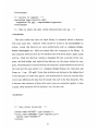
This thesis describes a suite of tools that were used to build an internet gateway,
with powerful 3D and 2D visualizations and intuitive, directed navigation, to an
expansive collection of geospatial imagery on the world-wide-web. The two driving
visions behind this project were: 1) to develop a system for automatically providing
flexible, modular and customizable infrastructure for navigating a hierarchical dataset
based on a simple and concise description of the paths users can take to reach items
in the dataset and 2) to create a visually exciting, interactive medium for members
of the machine vision community to explore the data in the City Scanning Project
Dataset and learn more about techniques the City Scanning Group is developing for
rapidly acquiring geospatial imagery with very high precision. In an effort to realize
these goals I have developed the DataLink Server, a system that provides navigation
and data retrieval infrastructure for a dataset based on a specification written in a
descriptive and coherent XML-based web navigation and data modeling language; a
geospatial coordinate transformation library for converting coordinates in virtually
any geographic or cartographic coordinate system; and a battery of visualization
applications for exploring the epipolar geometry, baselines, vanishing points, edge and
point features and position and orientation information of a collection of geospatial
imagery. These tools have been successfully used to deploy a web interface to the
more than 11,000 geospatial images that make up the City Scanning Project Dataset
collected by the MIT Computer Graphics Group.
Thesis Supervisor: Seth Teller
Title: Associate Professor of Computer Science and Engineering
3
4
Acknowledgments
Patience is the cardinal virtue of any good teacher, and, therefore, I would first like to
acknowledge my thesis advisor, Prof. Seth Teller, who, despite the impressive number
of students, projects and courses he supervises, still finds time to sit down with any
one of his students to share pointers about such humble subjects as debugging with
gdb and working with a UNIX shell as eagerly as he provides insights on graphics
algorithms, mathematics and other "hard-core" topics of computer science. I must
also thank Mom for her unfaltering support and encouragement, Sis for her ever
consummate advice, my brother Eric for restraining himself from dissuading me from
coming to MIT and Dad, to whom I owe my love of the outdoors and my respect for
the natural world. I should thank Prof. Patrick Henry Winston for reinvigorating in
me a passion for real science and Professors Alan Lightman, Anita Desai and David
Thorburn for all the distractions in fiction, literature and film.
Although I've never met him, Douglas Adams deserves recognition for impressing
upon me the subtle wisdom of cynicism at a very young age (which was further
cultivated by Kurt Vonnegut and Mark Twain, among others), and special thanks
is due to The Clash and Rancid for creating the quality punk rock albums that
provided much of the acoustical accompaniment to this work. On that note, while
making a conscious effort not to make this read too much like the liner notes of a
CD, I'd like to briefly mention: The Talking Heads, Nirvana, The Cure, The Spin
Doctors, Counting Crows, Train, Brahms, Mozart, Beethoven, Gershwin, Copland,
Isabelle Allende, Gabriel Garcia Marquez, Jim and William Reid, Jake Burton and
the seminal noise acoustics band Sonic Youth.
And now for the real funky stuff...
5
6
Contents
1
1.1
1.2
2
15
Introduction and Background Information
. 15
Background Information ........................
1.1.1
Image Acquisition and Post-processing Stages . . . . . . . . .
16
1.1.2
Description of the Existing Interface
. . . . . . . . . . . . . .
18
Overview of the Extended Interface . . . . . . . . . . . . . . . . . . .
23
1.2.1
The DataLink Server . . . . . . . . . . . . . . . . . . . . . . .
23
1.2.2
The Geospatial Coordinate Transformation Library . . . . . .
25
1.2.3
Other Minor Extensions and Improvements . . . . . . . . . . .
27
29
The DataLink Server
2.1
The DataLink Server Maps Virtual Navigation Hierarchies to Real Data 30
The DataLink Server Can be Accessed Programatically . . . .
33
Components of the DataLink Server . . . . . . . . . . . . . . . . . . .
33
2.2.1
Data and Navigation Models Define the Abstraction . . . . . .
34
2.2.2
The Core of the DataLink Server is the DataLinkServlet
. .
39
2.2.3
The Front End Consists of Content Handlers . . . . . . . . . .
39
2.1.1
2.2
3 Modeling Data and Directing Navigation Using XML
45
3.1
The Model Definitions are Described in XML
. . . . . . . . . . . . .
45
3.2
A Block Level Description of the Model File . . . . . . . . . . . . . .
46
. . . . . . . . . . . .
48
. . . . . . . . . . . . . . . . . . . . . . .
48
Creating a Data Model . . . . . . . . . . . . . . . . . . . . . . . . . .
48
3.3
3.2.1
An XML Schema is Used For Validation
3.2.2
Reserved Characters
7
3.4
3.3.1
Data Vertex Type Definitions . . . . . . . . . . . . . . . . . .
49
3.3.2
Declaring Data Vertex Instances . . . . . . . . . . . . . . . . .
55
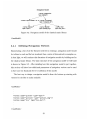
Writing a Model To Direct Navigation
3.4.1
3.5
4
. . . . . . . . . . . . . . . . .
58
Defining Navigation Vertices . . . . . . . . . . . . . . . . . . .
59
Chapter Summary
71
73
Content Handlers
4.1
Content Handlers Are JSPs, Servlets or HTML Documents . . . . . .
73
4.2
The Format of DataLinkServlet Requests . . . . . . . . . . . . . . .
74
4.2.1
The history Parameter . . . . . . . . . . . . . . . . . . . . .
75
Data Structures for Content Handlers . . . . . . . . . . . . . . . . . .
76
4.3
4.3.1
4.4
The DataLinkServlet Communicates to Content Handlers Using the curPathBean . . . . . . . . . . . . . . . . . . . . . . .
76
4.3.2
Data Structures for Attributes . . . . . . . . . . . . . . . . . .
77
4.3.3
Data Structures for Branches
. . . . . . . . . . . . . . . . . .
79
The DataLinkDispatcher Is Used to Format Requests to the DataLink
Server .......
..
.......
.....
............
..
.. .
79
. . . . . . . . . .
82
4.5
Making Menus With the BranchHistoryScripter . . . . . . . . . . .
83
4.6
Chapter Summary
86
4.4.1
5
. . . . . . . . . . . . . . . . . . . . . . . . . . . .
View Requests vs. View Resource Requests
. . . . . . . . . . . . . . . . . . . . . . . . . . . .
87
Operation of the DataLink Server
5.1
Data Structures for Curbing Computational Complexity
. . . . . . .
87
5.2
DataLink Server Requests Come in Two Flavors . . . . . . . . . . . .
88
5.2.1
View Requests
89
5.2.2
View Resource Requests
5.2.3
Specifying Abstract State Values
5.3
5.4
. . . . . . . . . . . . . . . . . . . . . . . . . .
. . . . . . . . . . . . . . . . . . . . .
90
. . . . . . . . . . . . . . . .
90
How the DataLink Server Handles View Requests . . . . . . . . . . .
91
5.3.1
How the Navigation Layer Handles a Select Vertex Request .
92
5.3.2
How the Data Layer Fetches the Branches for a Data Type .
95
How the DataLink Server Handles View Resource Requests . . . . . .
8
98
6
The Geospatial Coordinate Transformation Library
101
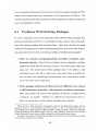
6.1
Problems With Existing Packages . . . . . . . . . . . . . . . . . . . . 102
6.2
GCTL Makes Reference Frames Explicit . . . . .
103
Design Principles of GCTL . . . . . . . . .
105
6.2.1
6.3
6.4
6.5
GCTL Understands Five Types of Coordinates .
106
6.3.1
107
Datums are Models of the Earth's Surface
. . . . . . . . . . . . . . . . . . . .
111
6.4.1
GCTL Data Types . . . . . . . . . . . . .
111
6.4.2
Defining Local Grid Coordinate Systems .
112
6.4.3
GCTL Can Convert Between Geodetic and Geocentric Coordi-
Using GCTL
nates . . . . . . . . . . . . . . . . . . . . .
113
. . . . . . .
115
6.4.4
GCTL Can Do Datum Shifts
6.4.5
GCTL Can Make Maps With Cartographic Projections . . . .
Chapter Summary
. . . . . . . . . . . . . . . . . . . . . . . . . . . . 120
7 Advanced Features of the Extended Web Interface
7.1
119
121
Enhanced Visualizations . . . . . . . . . . . . . . . . . . . . . . . . . 121
7.1.1
Extensions to the Map Viewer . . . . . . . . . . . . . . . . . . 122
7.1.2
Extensions to the Node Viewers . . . . . . . . . . . . . . . . . 124
7.1.3
New Global Visualizations . . . . . . . . . . . . . . . . . . . . 130
7.1.4
The New Web Interface Has Support For Radiance Encoded
Im ages . . . . . . . . . . . . . . . . . . . . . . . . . . . . . . . 134
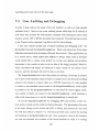
7.2
Content Handlers Can Perform Data Caching . . . . . . . . . . . . .
7.3
User Auditing and Debugging . . . . . . . . . . . . . . . . . . . . . . 138
136
8 Contributions and Concluding Remarks
141
A The DataLinkDispatcher API
145
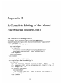
B A Complete Listing of the Model File Schema (models.xsd)
159
9
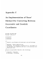
C An Implementation of Toms' Method For Converting Between Geocentric and Geodetic Coordinates
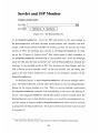
D Source Code For the OutputStreamServer and MonitorServiet
165
169
D.1 OutputStreamServer.java .........................
169
D.2 MonitorServlet.java ............................
176
10
List of Figures
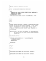
1-1
A screen-shot of the Map Viewer zoomed in to show node 104
. . . .
19
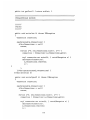
1-2 A screen-shot of the Mosaic Viewer enhanced with some of the extensions described in this thesis . . . . . . . . . . . . . . . . . . . . . . .
1-3
21
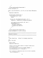
A screen-shot of the Epipolar Viewer comparing the geometry of two
views of The Great Sail . . . . . . . . . . . . . . . . . . . . . . . . . .
22
2-1
Interactions between the abstraction layers of the DataLink Server . .
31
2-2
A simple set of models for a classical music library . . . . . . . . . . .
35
2-3
Architecture of the DataLink Server . . . . . . . . . . . . . . . . . . .
40
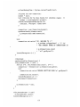
2-4
How the content handler for the composer vertex might format the
data for a composer . . . . . . . . . . . . . . . . . . . . . . . . . . . .
2-5
41
A screen shot of the content handler for the node vertex of the City
dataset........
...............
....................
42
3-1
Data model of a classical music library . . . . . . . . . . . . . . . . .
55
3-2
Navigation model of the classical music library . . . . . . . . . . . . .
59
3-3
Listing of the classical lib vertex
. . . . . . . . . . . . . . . . . .
61
3-4
Another listing of the classical lib vertex . . . . . . . . . . . . . .
62
4-1
Screen shot of a navigation context menu . . . . . . . . . . . . . . . .
83
5-1
Data paths through the DataLink Server . . . . . . . . . . . . . . . .
92
6-1
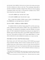
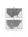
NAD83 - NAD27 datum shifts in arc seconds . . . . . . . . . . . . . .
117
7-1
The new Map Viewer . . . . . . . . . . . . . . . . . . . . . . . . . . .
123
11
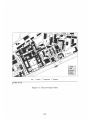
7-2
Screen shot of the Map Viewer zoomed in on the Green Building nodes 124
7-3
The sphere viewport window . . . . . . . . . . . . . . . . . . . . . . .
125
7-4
The heads-up display . . . . . . . . . . . . . . . . . . . . . . . . . . .
126
7-5
Edge and Point Feature Display . . . . . . . . . . . . . . . . . . . . . 127
7-6
An epipolar viewing of Building 18 with distance markings on the epipoles 128
7-7
Vanishing points visualization of the nodes along Mass. Ave. . . . . .
131
7-8
The node viewers' vanishing point visualization
132
7-9
The Map Viewer's baselines visualization . . . . . . . . . . . . . . . . 133
. . . . . . . . . . . .
7-10 The node viewers' baselines visualization . . . . . . . . . . . . . . . .
134
7-11 The MonitorServlet . . . . . . . . . . . . . . . . . . . . . . . . . . .
139
12
List of Tables
3.1
Reserved characters . . . . . . ..
. . . . . . . . . . . . . . .
48
3.2
Valid state pairings listed by example . . . . . . . . . . . . .
53
3.3
String format expression tokens used by the DataLink Server
55
3.4
Default values of navigation vertex parameters . . . . . . . .
65
4.1
NavPathBean routines for use in content handlers
. . . . . . . . . . .
77
4.2
Map data structures for holding attribute sets . . . . . . . . . . . . .
78
4.3
BranchClass routines for use in content handlers
. . . . . . . . . . .
80
4.4
Branch methods for content handlers . . . . . . . . . . . . . . . . . .
80
4.5
Other useful methods provided by the DataLinkDispatcher
. . . . .
81
6.1
GCTL Datum Classes
6.2
GCTL Ellipsoid Classes
. . . . . . . . . . . . . . . . . . . . . . . . .
109
6.3
GCTL NADCON Grids
. . . . . . . . . . . . . . . . . . . . . . . . .
119
. . . . . . . . . . . . . . . . . . . . . . . . . . 108
13
14
Chapter 1
Introduction and Background
Information
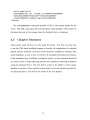
1.1
Background Information
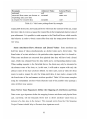
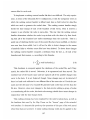
The goal of the City Scanning Project is to develop an end-to-end system for automatically acquiring 3D CAD models of urban environments under uncontrolled lighting
conditions (i.e. outside, under natural light) [Teller et al., 2001]. To achieve this goal
the City Group has constructed a sensor for automatically acquiring pose-augmented
imagery (image data coupled with position and orientation estimates) and a suite
of post-processing algorithms to refine the position estimates and extract intrinsic
parameters about building features. Using these tools the City Group has collected
over 500 sets of pose-augmented images which make up we believe to be the largest
dataset of geospatial imagery in existence.
The author had previously developed a world-wide-web based interface that allows
people from anywhere in the world to browse is dataset. This web interface included
a set of visualization tools that allow viewers to examine the quality of the data in
various post-processing stages and learn more about the process by which the data
is acquired [Bodnar, 2001]. This thesis outlines extensions and additions to the preexisting web interface in order to make it a powerful tool for analyzing the data. These
extensions make the web interface an easy-to-use exploration tool for members of the
15
general public to browse the data and learn more about the project, as well as a useful
tool for members of the City Group to validate the data, evaluate the performance
of the various processing stages and diagnose problems with the acquisition process.
This section outlines briefly what the reader needs to know about the image acquisition process and the pre-existing web interface. For more information about the
data, or the image acquisition and post-processing stages please refer to Calibrated,
Registered Images of an Extended Urban Area [Teller et al., 2001]. The previous version of the web interface is documented in A Web Interface for a Large Calibrated
Image Dataset [Bodnar, 2001].
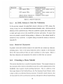
1.1.1
Image Acquisition and Post-processing Stages
Pose images are collected using a robotic sensor which consists primarily of a digital
camera mounted on pan-tilt head [De Couto, 1998]. The sensor is equipped with an
on-board GPS receiver, inertial motion sensors, a compass and wheel odometers which
are used to obtain reasonably accurate position and orientation estimates for each of
the images [Bosse et al., 2000]. When the sensor is activated at a given location, the
camera head rotates about a fixed optical center capturing between 20 and 71 images
tiling a portion of the sphere. One such collection of images, in combination with the
associated position and orientation information, is referred to as a node.
The images for each node are numbered sequentially beginning at zero. The position and orientation data for each image is logged in a camera file with an ID number
matching that of the associated image.' The camera files generated by the sensor are
what is referred to as the initialpose data.
When the sensor has been returned to the lab and the new nodes have been added
to the City database, an edge and point feature detection algorithm is applied to the
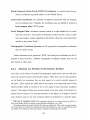
images. Then the initial pose files are subjected to a series of post-processing algorithms to refine the position and orientation estimates. All of these algorithms are
applied in a sequence of four post-processing stages: feature detection, mosaicing, ro'For more information about the format of a camera file and its contents, please refer to Calibrated, Registered Images of an Extended Urban Area [Teller et al., 2001].
16
tational alignment and translational registration/geo-referencing. Each of these stages
outputs a new set of camera files. The camera files from previous stages are kept in
a directory named after the post-processing stage that generated them. Each stage
can be described briefly as follows:
Feature Detection
During this stage edge and point features are extracted from each of the raw images
for use in later post-processing stages. This stage outputs edge and point feature
files.
Mosaic
At this stage the overlapping regions of the raw images are aligned. The images are
then blended together and resampled to form a spherical texture. The camera files
generated by this stage for a given node have improved orientation estimates relative
to each other. This stage outputs spherical textures and mosaiced camera files.2
Rotation
Edge features are used in the rotation phase to detect vanishing points (points where
families of parallel lines seem to converge when viewed from the optical center of the
node). The rotation process relies on the assumption that nearby nodes will share
some common vanishing points because they view some of the same building fagades.
The nodes are rotated in an attempt to align the shared vanishing points of adjacent
nodes. The result is further refinement of the orientation estimates. This stage outputs
vanishing points, node adjacencies 3 and rotated camera files. 4
2Please
see Spherical Mosaics with Quaternions and Dense Correlation, [Coorg and Teller, 2000]
for more information about the algorithms used in the mosaic stage.
3
A node is adjacent to any of its 3 (or sometimes 4) nearest neighbors and any other nodes within
a certain radius. Adjacencies are used to determine which nodes are likely to share common features,
such as vanishing points.
Urban Scenes
of Relative
Camera Rotations for
'See
Automatic Recovery
[Antone and Teller, 2000] for more information about the rotation stage.
17
Translation and Georeferencing
As a node is moved in a straight line, points on the spherical texture seem to emerge
from a common point as they move toward the viewer and converge at an antipodal
point as they move away from the viewer. These two points define a baseline. By
attempting to align baselines directions with the directions between two nearby nodes,
the translation process refines the relative position estimates of the nodes. Then
GPS estimates from the sensor are then used to scale, translate, and rotate the
camera positions to obtain new estimates that best fit the surveying data. This stage
outputs baselines for each pair of adjacent nodes and camera files with revised position
estimates. 5
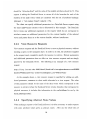
1.1.2
Description of the Existing Interface
The existing web interface consists of a number of HTML documents, CGI scripts
and Java applets which allow the user to browse the nodes, view the camera files and
feature files as well as view thumbnails of the raw images. It also includes a number
of visualization tools which allow the user to view the spherical textures, adjacencies,
epipolar geometry, node locations as well as many other features of the data. Finally,
it provides a remapping of the physical data structure of the dataset to a simpler
logical hierarchy more suitable for web-browsing.
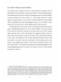
The Pre-existing Visualization Tools
At the core of the pre-existing web interface are the visualization applets. This section
describes the functionality of each of these applets briefly.
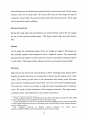
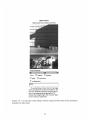
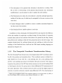
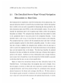
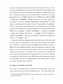
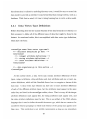
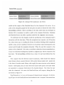
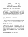
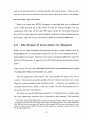
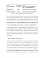
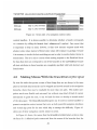
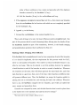
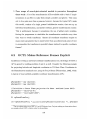
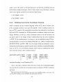
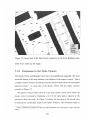
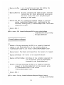
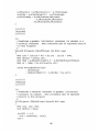
The Map Viewer
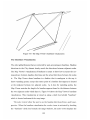
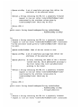
The Map Viewer shows the positions of the nodes superimposed
upon a map of campus. The node locations are shown in different colors corresponding
to their level of post-processing refinement. The Map Viewer can zoom in to show a
'See
Scaleable, Absolute Position Recovery for Omni-Directional Image Networks
[Antone and Teller, 2001] for more information about the translation/georeferencing stage.
18
Node's Position and Nearest Neiighbors
Key: 0 mosaiced
Show:
0 rotated
U baselines
Fl
*
vanishing points
F.adjacencies
view fll-scale map
The lines between nodes on the mini-map
connect each node to one ofits nearest
neighbors. Click on one of these lines to view
the epipolargeomeby of the two neighboring
nodes.
Figure 1-1: A screen-shot of the Map Viewer zoomed in to show node 104
close up view of a region of campus and can display adjacencies as lines which connect
node locations. Clicking on a node location redirects the user to a CGI generated
HTML document that displays information about the node, including images, links
to the pose and feature data as well as some other visualization tools. Clicking on an
edge between two nodes brings up the Epipolar Viewer (see below) for the implicated
node pair. Figure 1-1 is a screen-shot of the Map Viewer in mini-mode.
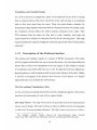
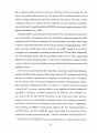
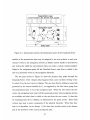
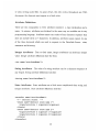
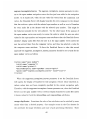
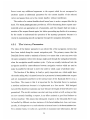
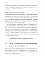
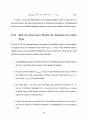
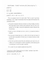
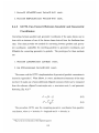
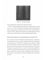
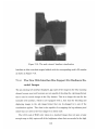
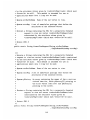
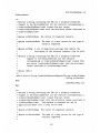
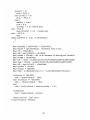
The Mosaic Viewer
This tool allows the user to view the spherical texture from
the point of view of the optical center of the node, looking out. Using the mouse
or the keyboard the vantage point can be rotated vertically or horizontally and the
field of view can be zoomed in or out. The Mosaic Viewer in the pre-existing interface is equipped with a gamma correction tool which compensates for the sometimes
strange coloration of the images (due to the fact that the images have a high dynamic
range logarithmically mapped onto a linear scale from 0-255) by boosting the color
saturation of the image.
Images in the city dataset are encoded using the SGI .rgb file format [Haeberli, 2002].
19
The .rgb format is not very web-friendly; it is neither supported by most web-browsers
nor the standard Java API. To ameliorate this problem, the existing toolkit used to
rely on a script that was run prior to the deployment of the web interface, which
generates .jpg encoded versions of the spherical textures. One of the extensions to the
pre-existing web interface was to augment the Mosaic Viewer (and the other applets
that use .rgb images) with a Java utility class, RGBImage, that can decode radiance
encoded .rgb images. This both eliminates the need to generate .jpg versions of the
images for web-viewing and the problems with color saturation (see Section 7.1.4 for
more information about the RGBImage class). Figure 1-2 is a screen-shot of the Mosaic
Viewer displaying some of the enhancements described in this thesis (see Section 7.1).
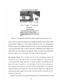
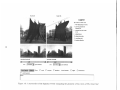
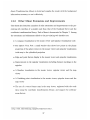
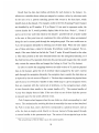
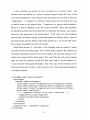
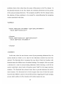
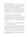
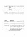
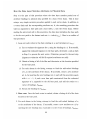
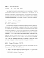
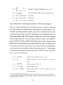
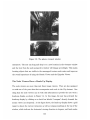
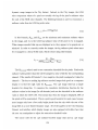
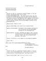
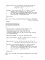
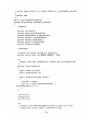
The Epiploar Viewer
The Epipolar Viewer is a two panel version of the Mosaic
Viewer. Each panel shows the view from one node of a pair of adjacent nodes. In each
view the neighboring node is marked by a blue cross. The Epipolar Viewer allows the
user to project a ray from the center of one view and see the corresponding line as
viewed from the neighboring node. For a pair of perfectly aligned nodes the ray should
appear to intersect the same points in space in both views, thus allowing the user
to visually inspect the quality of the position and orientation estimates generated by
the post-processing routines. The user can select, using a drop down menu, which set
of pose data to use when rendering the epipolar lines. This allows the user to observe
how the position and orientation estimates improve with each post-processing stage.
Figure 1-3 shows a screen shot of the Epipolar Viewer being used to examine two
views of The Great Sail.6 In Figure 1-3 the Epipolar Viewer has been augmented
with some of the advanced features described in this thesis (see Section 7.1).
6
Calder, Alexander The Great Sail. 1966 Massachusetts Institute of Technology, Cambridge.
20
Mosaic Viewer
(planar projection of spherical mosaic)
saturation threshold:
Show:
L edges
0
compass
C
baselines
[ intersections
. vanishing points
Status
To use the Mosaic Viewer click on the image
above and dragit to the desiredviewpoint. You
can also rotate the viepoint by using the arrow
keys or by draggingand droppingthe PO V
marker (the orange target). The z'and W'keys
zoom in and out, respectively.
Figure 1-2: A screen-shot of the Mosaic Viewer enhanced with some of the extensions
described in this thesis
21
Node 324
Node 326
Legend
O location of other node
POV (drag/drop to move)
point of projection of
epipolar line
epipolar line (with scale
-r
in m)
edge feature
0 edge intersection
*
vanishing point
+ baseline direction
saturation threshold:
Use
translated
Show Epipoe
r
saturation threshold:
Cl
pose estimate.
A
Show:
IT
scale
Use
r7 compass
|translated
pose estimate.
[T baselines
Show Features:
rT edges
IT
intersections
vanishing points
Status
Figure 1-3: A screen-shot of the Epipolar Viewer comparing the geometry of two views of The Great Sail
1.2
Overview of the Extended Interface
The extended interface has roughly the same look and feel as the original pre-existing
interface. It allows users to browse the dataset in nearly the same fashion as before
and view the data using improved versions of the visualization applets described in
the previous section. In addition to enhanced functionality, the new web interface is
backed by a new, powerful and versatile navigation infrastructure whose core is a Java
servlet package called the DataLink Server. A C++ static library for transforming
Earth coordinates has also been added to the visualization toolkit allowing the dataset
to be used in conjunction with data from outside sources expressed in almost any
geographic, geocentric, or cartographic coordinate system. This section gives a brief
overview of the DataLink Server, the coordinate transformation library and other
minor extensions and improvements that have been made to the pre-existing interface,
all of which will be described in greater detail in subsequent chapters.
1.2.1
The DataLink Server
For the pre-existing web interface, the abstraction between the organization of the
data presented to the user and its arrangement on the physical disk is provided by
a few Perl scripts. These scripts traverse the directory tree of the physical data and
generate symbolic links to the relevant files. They must be run prior to deployment
of the web site. The symbolic link trees re-map the complicated directory structure
of the physical data to a simpler hierarchy that is more suitable for browsing on the
web [Bodnar, 2001]. Although re-mapping the data in this way effectively provides
the desired abstraction, the symbolic links are problematic in that they must be
regenerated every time there are additions to the data.7 In addition, any changes in
'One might consider running these scripts in a crawler-like mode to automatically incorporate
additions and deletions. However, this involves both the creation and removal of symbolic links in
the public HTML directory of the web interface so it is likely to cause irritating 404 - Not Found
messages and other disruptions if the dataset is modified at the same time it is being browsed by
a user, due to the caching that is performed by most web browsers. Also, the DataLink Server is
capable of incorporating updates in real time, whereas the crawler scripts would have to be run
episodically.
23
the organization of the physical data or its layout on the web requires modification
of the Perl scripts themselves which necessitates, at a minimum, decent working
knowledge of the dataset, the operation of the scripts and the Perl programming
language.
The DataLink Server provides a more versatile solution to this problem. The Data
Link Server is a web application consisting of Java servlets and Java Server Pages
(JSPs) that provide an abstraction function between a particular web layout and
a physical data store. The DataLink Server allows a web designer to define one or
more alternative logical arrangements of the data using a simple XML-based modeling language. The hierarchical organization of these logical arrangements may be
completely different from the layout of the physical data. Using the XML description
of the web layout and a similar XML-based model of the physical data, the DataLink
Server automatically resolves the mapping between the logical hierarchy of the presentation layer and the location of the physical data on they fly as the information
is browsed by a user. In addition, the DataLink Server allows the web architect to
specify content managers, which are additional JSPs or servlets that generate the
HTML for presenting a particular datum, giving the web designer complete control
over the look and feel of the front end.
This infrastructure provides a number of key benefits over the pre-existing scriptgenerated architecture:
" As new data is added to the dataset it becomes instantly available for browsing
via the web interface because the mapping between the web layout and the
physical layout is resolved at run time.
" No broken links result from the renaming or removal of data because the
DataLink Server will only resolve mappings to existing physical data.
" Information about the layout of the presentation layer is centralized in a single
XML document, so reorganizing the entire web site can be done by editing a
single file.
24
"
The description of the physical data hierarchy is described in a solitary XML
file as well, so restructuring of the physical data hierarchy only necessitates
modifications to one document in order to update the web interface.
* The DataLink server allows the web architect to describe multiple logical hierarchies of the data, any of which may be navigated by the user to arrive at the
same data.
" Content Managers make it possible to create a modular customized fagade for
the front end of the interface.
" The DataLink Server handles updates in real time.
In addition to these advantages, the DataLink Server also improves the efficiency
of the web interface by employing a caching strategy for large blocks of commonly
accessed data (such as the locations of the nodes to be plotted by the Map Viewer)
and performs user auditing to help the City group keep tabs on the site's usage. The
complete details about the caching strategy and user auditing, as well as the inner
workings of the DataLink Server itself and the XML-based modeling language are
discussed in Chapters 2-4.
1.2.2
The Geospatial Coordinate Transformation Library
The City Scanning Project dataset uses a local tangent plane (LTP) coordinate system
for all of its position and orientation data. This coordinate system is defined by a
right handed set of axes with the x axis pointing east, the y axis pointing north
and the z axis pointing up (normal to the Earth) with units in meters. 8 The origin is
located at the position of the GPS base station antenna (on the roof of building NE43
in Tech Square) that the City group uses to obtain differential GPS measurements of
the nodes' placement. This coordinate system is used to provide the highest degree of
precision to position estimates acquired using differential GPS. The disadvantage of
8
This type of coordinate system is also sometimes referred to as an East North Up (ENU) or
East North Height (ENH) coordinate system [Hofman-Wellenhof et al., 1997].
25
this coordinate system, however, is that it is used only with the City group. For this
reason, the position information in the City group's LTP coordinate system is not as
useful to people browsing the data from outside the City group, who work in other
coordinate systems, as it could be if it were exported in a more well known coordinate
system like Earth-Centerd Earth-Fixed (ECEF) or lattitude-longitude-altitude (LLA)
[Hofman-Wellenhof et al., 1997].
Similarly, there is much data generated outside of the City group that would be of
use to its members. For example, there exist detailed floor plans and maps of the MIT
campus in AutoCAD format, maintained by the Department of Facilities, which could
be used to check data derived by the City Group's post-processing algorithms. These
maps, and other outside data sources, however, are usually expressed in one of the
commonly used cartographic coordinate systems such as US State Plane. Registering
the LTP coordinate system with the coordinate systems used in these maps would
help the City group validate its data. It could also be beneficial in merging the data
we have collected about the building exteriors with detailed information about the
building interiors.
There are, of course, limitless other ways that a coordinate transformation library
capable of unifying data expressed City group's internal LTP coordinate system and
the major coordinate systems used in mapping and surveying could be beneficial.
For this reason I have created the Geospatial Coordinate Transformation Library.
This coordinate transformation library is a static C++ library which can be linked
to any of the City group's existing software or new applications which provides the
capability to transform coordinates expressed in an arbitrary LTP coordinate system, such as the one used by the City group, to any of the most widely used geographic, geocentric and cartographic coordinate systems. The coordinate transformation library could be used in conjunction with an open source library (libgeotiff,
[remotesensing.org, 2000]) for exporting the images in the City Scanning Dataset to
GeoTIFF [Ritter and Ruth, 2000], the image format which is becoming the de facto
standard for encoding geospatial imagery.9 Chapter 6 describes the Geospatial Coor9
An extensive source of information about the GeoTIFF format is the official GeoTIFF website:
26
dinate Transformation Library in detail and supplies the reader with the background
information necessary to use it effectively.
1.2.3
Other Minor Extensions and Improvements
This thesis also describes a number of other extensions and improvements to the preexisting web interface of a smaller scale than that of the DataLink Server and the
coordinate transformation library. Each of these is documented in Chapter 7. Among
the extensions and refinements added to the pre-existing web interface are:
" A compass visualization in the mosaic viewer and epipolar visualization tools
" The Sphere View Port: a small window that shows how points in the planar
projection of the sphere texture in the mosaic viewer and epipolar visualization
tools map to the cylindrical projection
" Edge and point feature display in the mosaic viewer and epipolar visualization
* Improvements to the epipolar visualization including distance markings on the
epipoles
" A Baseline visualization in the mosaic viewer, epipolar viewer and the map
viewer
* A Vanishing point visualization in the mosaic viewer, epipolar viewer and the
map viewer
" The use of a vector format map in the map viewer, registered with the node
data using the coordinate transformation library, and support for arbitrary
zoom factors
<http://www.remotesensing.org/geotiff/geotiff.html>.
27
28
Chapter 2
The DataLink Server
The DataLink Server is designed to facilitate the development of an easily configurable
interface for navigating a vast data store on the web. It was created as a step toward
fulfilling the desire for a system that abstracts the true organization of the data by
providing a pliable set of virtual hierarchies which can be tailored to web navigation
while at the same time being easily maintainable by a web architect. Folding several
logical organizations of the data into one allows a user to explore the full multidimensionality of the data space. Such a system should give the user the capability
to navigate to the same piece of data though several alternate paths to accommodate
for the fact that various users will have different perceptions about what the logical
arrangement of the data should be, and it should only provide navigation options for
data that is physically present.
The DataLink Server takes several important steps towards realizing this goal.
It provides the web developer with centralized, easy-to-modify configuration mechanism: an XML document describing the physical data and the set of valid navigation
paths to be made available to users. It also supports a modular front end interface
constructed from JSPs, Java servlets and HTML documents called content handlers,
each of which handles the presentation of data at a particular set of locations within
the navigation hierarchy. The DataLink Server has been successfully deployed as the
backbone of the City Scanning Project Dataset where it facilitates the navigation of
the more than 11,000 geospatial images the City group has collected since the spring
29
of 2000 and the data we have extracted from them.
2.1
The DataLink Server Maps Virtual Navigation
Hierarchies to Real Data
The DataLink Server implements a three-level abstraction of the physical data. The
topmost abstraction barrier is created by the presentation layer, which is the interface
that is visible to the user and is responsible for formatting the data provided by the
lower abstraction layers into HTML or other web-browsable content. The next level
beneath the presentation layer is the navigation layer which is where the navigation
hierarchies are defined. The navigation layer describes what data should be visible
to the presentation layer at any given point in the navigation hierarchy. It also
describes where a user can go to next from the current location in the hierarchy.
The navigation layer has a contract with the presentation layer such that it will only
provide navigation options for data which is physically present. In order to ensure
that this covenant is fulfilled, the navigation layer interfaces with the data layer in
order to resolve the mappings between the virtual data abstractions in the navigation
layer and real physical data in the dataset. The data layer describes the physical
hierarchy of the data and defines the attributesof each type of datum which might be
present in the dataset. Attributes are bits of information such as image resolution,
source sensor, date of acquisition or any other properties of which should be presented
as selections that the user can use to locate specific data.
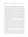
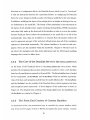
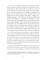
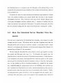
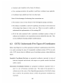
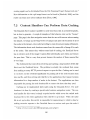
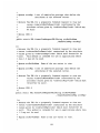
Figure 2-1 depicts the interactions between the three abstraction layers of the
DataLink Server. As the figure shows, the navigation layer can be thought of as a
directed graph, or network, in which each vertex represents a specific location in the
navigation hierarchy. Leaf vertices, shown in Figure 2-1 as darkened circles, represent
physical resources in the dataset such as images, data files etc. All other vertices in
the navigation graph correspond to locations in the virtual navigation hierarchy and
may or may not be associated with locations in the physical data hierarchy. A content
30
Presentalion Layer
Content Handlers: JSPs, Servlets, HTML Applets...
gation Layer
y
S
Data Layer
2
.........
........
Figure 2-1: Interactions between the abstraction layers of the DataLink Server
handler in the presentation layer may be assigned by the web architect to each nonresource vertex in the navigation network (a default content handler is provided for
any vertices for which the web architect elects not create a custom content handler).
Edges in the navigation graph tell the DataLink Server what data is visible to the
user at a particular vertex in the navigation hierarchy.
The two gray arrows in Figure 2-1 show the primary data paths through the
DataLink Server. Path 1 depicts what happens when a user currently viewing vertex
V selects V2 as the next vertex to display. The user does this by clicking on some link
generated by the content handler for
1, as
suggested by the blue arrow going from
the presentation layer to V2 in the navigation layer. When the user selects the new
vertex, the navigation layer must tell the presentation layer what navigation options
are available and what data is visible to the user from the new vertex. It does this
by examining each of V2's children, as illustrated by the green arrows. These child
vertices may map to some components of the physical hierarchy. What data they
map to is dependent on two things: 1) the data that actually exists in the dataset
and 2) the attributes of the current navigation path.
31
Recall that the data layer defines attributes for each datum in the dataset. Attributes are variables whose values get assigned at runtime, either by selections made
by the user or by a pattern matching process that occurs in the data layer, which
identify data in the dataset. For example, nodes in the City Scanning Project Dataset
are identified by an ID number. If V2 in Figure 2-1 was used to represent nodes, the
content hander for V would probably display links of the form "Node 1", "Node 2"
and so on for every node that exists in the dataset,' provided the set of nodes visible
to the user at this point was not constrained by other attribute values accumulated
along the user's current path through the navigation graph. The user would move to
V2
in the navigation hierarchy by selecting one of these links. When the user makes
one of these selections a value for the node ID attribute would be assigned. For example, if the user clicked on the link for "Node 2" node ID would bound to the value
2. This value persists as the user descends further into the navigation hierarchy, so if
the child vertices of V2 represent directories for pose data and images then they would
only contain the camera files and images that belong to Node 2 in City dataset.
In order to resolve the mappings between the child vertices of V2 and the physical
data in the dataset, given the set of attribute values assigned by the user's current
path through the navigation hierarchy, the navigation layer consults the data layer as
is depicted by the red arrows of Figure 2-1. The data layer examines the physical data
and returns a set of branches -handles to data which map to a given navigation vertex
that are consistent with the current set of attributes- to the navigation layer, which
in turn forwards these results to the content handler of V2 . The content handler of
V2 may then display them as links. If the user clicks on one of these links the process
is repeated anew for the newly selected vertex.
Path 2 depicts what happens when the user clicks on a link corresponding to a leaf
vertex. The mechanism for resolving this data is essentially the same as that described
for Path 1 except that, since a leaf vertex corresponds to a physical resource, such as
a file, the data is simply served directly to the user instead of being passed through
a content handler in the presentation layer. The action of the navigation layer is also
'The actual format of the the links is up to the content handler.
32
minimal in this case. It simply requests the appropriate data from the data layer and
then passes it along to the user.
2.1.1
The DataLink Server Can be Accessed Programatically
For simplicity, the previous discussion referred to the client of the DataLink Server
as the user. However, requests to the DataLink Server are made using the GET
or POST protocols, which means that the DataLink Server can also be accessed
programatically like a CGI application. This gives content handlers or other web
applications the ability to locate data within a dataset "behind the scenes" in order
to generate more dynamic content without any code for locating physical resources
being hard-wired into the actual web content. The DataLink Server package includes
a Java API which can be used to create properly formatted requests for items in
the navigation hierarchies given an appropriate set of attributes. Section 4.4 and
Appendix A give the complete details of the API for formatting requests to the
DataLink Server. As we'll see in Section 5.2 the typical format for DataLink Server
requests using the GET protocol looks like:
DataLink?view=node&dataset=all-nodes&nodeId=l1&history=dataset:all-nodes
2.2
Components of the DataLink Server
The DataLink server is comprised primarily of five discrete components. This modular architecture is essential to achieve the high degree of customizability provided
by the DataLink Server. All of these components interface with one central application, the DataLinkServlet, which handles the processing of requests. Only the
DataLinkServlet itself and the software behind its API are off-limits to developers.
All of the other components are created or extended by web developers to implement
a custom web application. The idea is that the web developers only have to describe
how the web site should be laid out as well as what functionality it should provide,
and the DataLink Server infrastructure should take care of the rest. The follow33
ing sub-sections describe each of the essential components of the DataLink Server in
detail.
2.2.1
Data and Navigation Models Define the Abstraction
The abstraction function provided by the DataLink Server is defined by a pair of
directed graphs called the navigation model and the data model. Section 2.1 and
Figure 2-1 have already given some sense of the nature of the navigation model. As
we have seen so far, the navigation model consists of vertices which represent locations
in the virtual navigation hierarchies. Most of these vertices really represent some type
of datum in the physical dataset. This data type may be a resource, such as an image
or a data file type, or, it may be a type of vertex in the physical data hierarchy, such
as one of the node directories that contains all of the data for a particular node in the
City dataset. Navigation vertices, however, need not correspond to a real physical
datum at all. They may simply exist for the purpose of guiding the user's navigation
by assigning values to attributes, or they may be used for generating a particular
view of some subset of the data.
The navigation model is coupled with the data model to resolve the mapping
between the virtual data hierarchies and the real physical data. Vertices in the data
model correspond to items in the dataset. Edges in the data model graph describe
the hierarchical relationships between these elements. In particular, if there is an
edge from data vertex V to data vertex V2 then V inherits the attributes of V2 .
Every vertex in the data model is an instance of a data vertex type. Each unique kind
of datum in the dataset is represented by its own data vertex type whose definition
contains information about the names and types of attributes associated with that
particular datum. There may be multiple instances of a single data vertex type in
the data model.
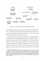
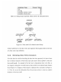
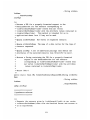
The illustration in Figure 2-2 should help to clarify how the navigation model and
data model abstractions work together. Figure 2-2 shows a simple set of models that
describe the web interface to an imaginary classical music library. On disk, the physical hierarchy of the library consists of a root directory which holds a subdirectory for
34
M
Navgaflon Model
DataModel
<name="root",
<name="DATASEr,
type="dataset">
-
-
-
datselName
-
-ype="dataset">
name=Nopus number">
<name="COMPSER",
type="composer_dir">
composerName
<name=-composer-,
ype="composerdir">
<name="pleces",
-ype="mp3N>
<name="MUSiC_FILES",
type="musicdir">
<name="BIO_DIR",
type = "blodir">
<name=portralt",
type="portahtJmg">
<name="PIECES",
<name="BIOGRAPHY",
<name=PORTA",
type="mp3">
opusNum o
type=Nblo doc">
type="portaltimg">
<name="bio",
ype=Nblo doc">
pleceName
Figure 2-2: A simple set of models for a classical music library
each composer in the library.2 Each composer directory contains two subdirectories.
One is a "biography" directory which holds a document about the life of the composer and an image of the composer's head. The other is a "music" directory which
contains audio files of pieces written by the composer.
The navigation model re-maps this directory structure to a slightly different set
of hierarchies. The user can begin browsing the dataset by selecting the name of a
composer, causing the system to visit the composer vertex. Once that selection is
made the user will see a listing of pieces penned by the selected composer as well
as a biographical sketch and a mug-shot. Clicking on the name of a piece will then
download that recording. An alternative route that the user could take through the
dataset is to begin by selecting the opus number of a piece to find. This would take
2
The data models discussed in this document will typically be models of directory trees. This
is a reflection of the first target application of the DataLink Server: purveying the navigation
infrastructure for the City Scanning Project Dataset, which is stored in an elaborate directory
structure. It should be noted, however, that the data model is merely an abstraction and that,
although the software implementing this abstraction is tailored to modeling directory trees, it would
be easy to extend the data model to provide an interface to any hierarchical data storage system,
such as a database.
35
the user to the opus number vertex. Figure 2-2 does not completely specify what
the behavior of the system should be at this point, but there are two possibilities:
1) The system could display link for every piece in the dataset with the selected
opus number as well as a link for every composer in the dataset. 2) The system
could display only the the links to the composer branches and omit the links to the
audio files because the attributes accumulated along the path traversed thus far are
not enough to completely specify the path to any piece of music. It is possible to
configure navigation vertices with either behavior.
Before reading any further, be sure to note that the edges in the data
model and navigation model graphs point in opposite directions. In Figure 2-2 the edge going from the PIECES data vertex to the MUSIC-FILES vertex indicates that MUSICFILES is the parent directory of the audio files which correspond
to MUSICFILES. This means that pieces inherit all the attributes of MUSIC-FILES,
COMPOSER and COMPOSERDATASET, the ancestor vertices of PIECES, so a piece in the
classical music library has values for the datasetName, composerName, opusNum and
pieceName attributes (In Figure 2-2 the attributes for a given data vertex type are
listed under each instance of that vertex type).
The edge from the opus number
navigation vertex to the pieces vertex 3 in the navigation model, on the other hand,
means that pieces is the child of opus number; any audio files visible to the user
located at vertex opus number in the navigation hierarchy must have the same opus
number as the branch of opus number that the user selected to view.
The reason for this disparity is that it makes the implementation of the models in
the DataLink Server much simpler and more efficient. Chapter 5, which discusses the
implementation of the DataLink Server, will elucidate the logic behind this design,
but, for now, the basic intuition is that the user will navigate a hierarchy from the top
down, accumulating attributes which make the subset of the data in consideration
3Throughout this thesis I have adopted the convention that data vertex names will be written in
UPPERCASE whereas navigation vertex names will be completly lowercase in order to differentiate
between data and navigation vertices which have the same names. The names of vertices in the
actual model files do not have to adhere to this convention, and they may contain any virtually any
character apart from some special characters which are described in Chapter 3.
36
more and more narrow.
When trying to map attributes to physical data in the
data model, however, the system will never be concerned with the children of a
vertex. Instead it will need to examine the vertex's ancestors in order to determine
the attributes it may have, or it may have to enumerate the ancestors to reconstruct
a path to the physical data.
Interactions Between the Data and Navigation Models
The dashed blue lines in Figure 2-2 show one way in which the navigation model
interfaces with the data model to retrieve the physical data. The specification for
navigation vertices which map directly to physical data in the data model include a
type field which gives the name of the corresponding data vertex type in the data
model. When the navigation layer explores a child vertex of the currently selected
vertex (as shown by the green arrows in Figure 2-1) which is mapped to a data vertex
type, T, to see which elements of type T (if any) should be made visible to the
presentation layer, it makes a request to the data layer for all branches of type T
which are consistent with the current set of attribute values. The data layer then
looks for every instance of data vertex type T in the data model, and examines its
ancestry to construct a chain of data vertices from each matching data vertex to the a
root vertex in the data hierachy.4 The set of chains revealed by this process describes
all of possible paths to data of type T. The data model then returns a set of complete
attribute bindings for all the paths in this set which are consistent with the attribute
values specified by the navigation layer.
For example, suppose our music library contained only four pieces: the Brahms
sonatas for clarinet and piano no. 1 and no. 2 op. 120, Beethoven's symphony no. 2
op. 36 and Vivaldi's The Four Seasons op. 8. Selecting the branch of navigation vertex
composer for "Brahms" from the root vertex would define the current set of attribute
bindings to be {composer = "Brahms",
datasetName = "classical"}. The navi-
gation layer would then examine each of the child vertices of composer to determine
4 There is no restriction on the number of root vertices that may exist in the data model.
37
the next set of navigation options that should be made available to the user. To discover the possible options for vertex pieces the navigation layer would request the set
of all branches for data vertex type mp3 for which composer = Brahms from the data
layer. The data layer would then look in the data model for instances of vertex type
mp3 and find only one, PIECES. The chain for the PIECES vertex looks like PIECES
-4
MUSIC-FILES
-*
COMPOSER
-*
DATASET which, given the current attribute val-
ues, expands to a the path /classical/Brahms/music-files/Brahms-*-op.*.mp3,
where the asterisks denote the unknown values of the pieceName and opusNum attributes.5 The data layer matches this path to the two Brahms pieces in the dataset
and returns the following sets of attribute bindings as the possible branches for the
PIECES vertex: {composer = "Brahms", datasetName = "classical", pieceName
=
"Sonata for Clarinet and Piano no. 1", opusNum = 120} and {composer =
"Brahms", datasetName = "classical", pieceName = "Sonata for Clarinet and
Piano no. 2", opusNum = 120}.
Another way which the navigation model might synchronize with the data model
for vertices that do not map directly to data vertex types is illustrated by the green
arrow in Figure 2-2. This arrow depicts the opusNum attribute being promoted to a
higher level in the navigation hierarchy. When the navigation layer explores the opus
number vertex it will try to determine all possible values for the promoted opusNum
attribute, given the current set of attribute values. It will do this by consulting with
the data layer about the possible values for this attribute in a way that is analogous
to requesting all valid branches for the PIECES vertex and extracting from this the
set of all possible values for the opusNum attribute, each of which will be presented
as a distinct navigation option to the user.
The Models are Defined Using XML
The models for a particular dataset are defined in an XML document which is completely separate from the rest of the DataLink Server.
The model definition file
5The details about how the DataLink Server maps attribute values to directory and file names
will be given in Chapter 3.
38
functions as a configuration file for the DataLink Server which is used to "bootstrap"
it with the abstraction function for a particular dataset, so configuring the DataLink
Server for a new dataset is chiefly a matter of writing a model file for the new dataset.
In addition, modifying the layout of an existing site is as simple as altering a few vertex definitions in the model file. The beauty of this mechanism is that alterations to
the layout of web interface don't require rewriting the hyperlinks, HTML documents
and scripts that make up the front-end of the interface in order to re-wire the website
because DataLink Server follows the specification in the model file to do all of this
automatically. Also, data can be added to or removed from the dataset without the
need to regenerate any part of the web site's infrastructure since all of the navigation
options are determined dynamically. The content handlers to be used for each navigation vertex are also specified within the model file. Chapter 3 will have more to
say about the navigation and data model abstraction and the XML-based modeling
language that is used to define them.
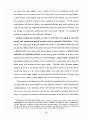
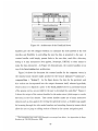
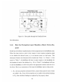
2.2.2
The Core of the DataLink Server is the DataLinkServlet
At the heart of the DataLink Server is the DataLinkServlet Java servlet, which
provides the navigation/data location infrastructure needed to drive a web interface
based on the specification captured in the model file. The DataLinkServlet is backed
by two components, the DataModel and the NavModel which are software representations of the data and navigation models from the model definition file. The DataModel
and the NavModel are the modules of the DataLink Server which implement the data
and navigation layers respectively. A block diagram of this architecture is shown in
Figure 2-3. The detailed inner-workings of the DataLinkServlet, the DataModel and
the NavModel are related in Chapter 5.
2.2.3
The Front End Consists of Content Handlers
As mentioned earlier, the presentation layer is controlled by content handlers which
may be Java server pages, servlets or HTML documents (for static content). Content
39
DataLinkServlet
Navigation Layer
NavModel
Data Layer
DataModel
Figure 2-3: Architecture of the DataLink Server
handlers give the web designer freedom to customize the look-and-feel of the web
interface and flexibility in controlling the way the data is presented to the user. A
content handler could simply present links to the raw data, much like a directory
listing or it may incorporate Java applets, Javascript, DHTML or other means to
make the data interactive. As Figure 2-3 demonstrates, the content handlers sit on
top of the DataLinkServlet architecture.
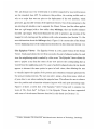
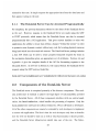
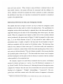
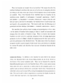
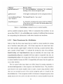
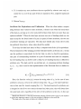
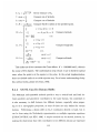
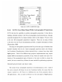
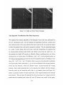
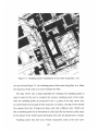
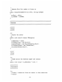
Figure 2-4 shows the document the content handler for the composer vertex in
the classical music dataset might produce for the branch {dataset="classical",
composerName = "Brahms"}. As the figure shows, the data for the portrait and
bio vertices are incorporated into the output document itself, whereas hyperlinks,
whose action is to dispatch a query to the DataLinkServlet for a particular branch
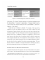
of the pieces vertex, are provided for the user to download the audio files.' Figure 25 shows the output of the content handler for the node vertex (which maps to a node
directory) in the City dataset. This content handler makes use of many interactive
elements such as Java applets for viewing the spherical texture, a clickable map applet
for browsing through the other node branches and cascading Javascript menus which
allow the user to jump to sibling vertices of those in the current navigation path.
6
The biographical text used in this example is an excerpt from Music: An Appreciation by Roger
Karmien, pp. 256-258 [Karmien, 1999].
40
Johannes Brahms
Works
Sonata for Clarinet and Piano no. 1 op. 120
Sonata for Clarinet and Piano no. 2 op. 120
Biography
"Johannes Brahms (1833-1897) was a romantic who breathed new life
into classic al forms. He was born in Hamburg, Germany, when his
father made a precarious living as a bass player. At thirteen, Brahms led
a double life: during the day he studied piano, music theory, and
composition; at night he played dance music for prostitutes and their
clients in water front bars.
"On his first concert tour, when he was twenty, Brahms met Robert
Schumann and Schumann's wife Clara, who were to shape the course
of his artistic and personal life. The Schumanns listened enthusiastically
to Brahm's music, and Roberts published an article hailing young
Brahms as a musical messiah.
"As Brahms was preparing new works for an eager publisher,
Schumann had a nervous collapse and tried to drown himself When Schumann was committed to an asylum,
leaving Clara with seven children to support, Brahms c ame to live in the Schumann home. He staye d for two
years, helping to care for the children when Clara was on tour and becoming increasingly involved with
Figure 2-4: How the content handler for the composer vertex might format the data
for a composer
41
This repository is still underdevelopment. We would appreciateyour feedback.
Current Path: 'all-nodes-fixed' Dataset/Node I Node 34
Node 34
Acquired on May 18, 2000 2:59 PM
Node Viewed as a Cylindrical Mosaic
Node's Position and Nearest
Neighbors
Key 9 mosaiced
Show:
IQ
F
0 rotated
baselines
F
Mosaic Viewer
(planar projection of spherical mosaic)
0 translated
vanishing points
R adjacencies
view full-scale map
between nodes on the
saturation threshold:
mini-map connect each node to one of
its nearest neighbors. Click on one of
these lines to view the epipolar
geometry of the two neighboringnodes.
Images
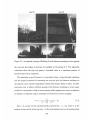
The images you see on this page constitute one node from the City Scanning Project dataset. The raw images seen at the
bottom of this page share a common optical center but are rotated into various orientations that together tile a hemisphere. During
the mosaic stage of post processing, these images are more accurately aligned with each other and combined to form the spherical
texture seen above. The spherical texture is better viewed using the Mosaic Viewer at the right, which allows you to view the
node from its optical center and rotate the viewing angle along the horizontal and vertical axes.
The images in the City Scanning ProjectDataset are all high dynamic range (HDR) images. Although the images are
encode d using the lossless SGI .rgb format, with color values ranging from 0-255, these values actually represent the log of the
true radiance values. The following equation captures the relationship between the .rgb pixel values and the corresponding
saturation threshold:
Show:
F edges
F
F
compass
F
F intersections
vanishing points
Status
Figure 2-5: A screen shot of the content handler for the node vertex of the City dataset
baselines
The API for Writing Content Handlers
The DataLink Server package provides two crucial classes for interfacing with the
DataLinkServlet that facilitate writing content handlers. The DataLinkDispatcher
class implements about 20 static methods for formatting requests to the DataLinkServiet and processing the data returned by it. These include methods for sorting
branches, opening streams to resource files via the DataLinkServlet and formatting
URLs or hyperlinks that access DataLinkServlet given a set of attribute values,
which may be encoded in one of serveral different types of data structures.
The DataLink Server also includes a class for formatting special context navigation
menus, BranchHistoryScripter, for use in content handlers. The menus created
by this class are activated by mousing over the name name of one of the branches
visited along the user's current path through the navigation hierarchy, which are
listed at the top of the page, or wherever the author of the content handler decides
to place them, and enumerate all of the other alternative branches the user could
have chosen at that point in the path. Selecting one of these options jumps to that
branch. In the sample screen in Figure 2-5 the user has activated the context menu
for the node branch. 7 The complete documentation of the DataLinkDispatcher and
the BranchHistoryScripter are located in the chapter devoted to content handler
development: Chapter 4.
7 There are more than 500 nodes in the City dataset, which is why the context navigation menu
for nodes only lists two options: one for the currently selected node and one which warps the user
back to the next higher level in the hierarchy, the dataset vertex, in order to choose another. When
there are only a few alternatives the menus can display them all. Parameters in the model file
allow the developer of the web site to specify which of these alternatives is appropriate for a given
navigation vertex. As is to be expected, there are performance issues associated with allowing the
full listing capability for vertices which could potentially have a large number of branches.
43
44
Chapter 3
Modeling Data and Directing
Navigation Using XML
In this chapter you will learn about the XML-based modeling language for describing
a dataset and controlling the behavior of the navigation layer of the DataLink Server.
You will learn how a data model describes how to extract the salient properties of
the data from a hierarchical dataset, as well as how the navigation layer uses the
attributes of the data as the pivots about which navigation is guided. You will see
how the navigation model outlines the behavior of the navigation layer and how it
determines the type of information that is passed to the presentation layer. Each
of the modeling constructs in this chapter is illustrated with concrete pedagogical
examples or real samples from the City dataset, and, by the end of it, you will have
acquired all of the knowledge necessary to begin designing the architecture of powerful
web gateways to large datasets.
3.1
The Model Definitions are Described in XML
The modeling constructs used to control the DataLink Server are written in XML 1
XML was chosen as the basis of the modeling platform in lieu of some custom language
1The
definitive
resource
on
XML
is
Extensible Markup
[The World Wide Web Consortium, 2002a], <http://www.w3.org/XML/>.
45
Language
(XML),
and file format because it has a number highly desirable qualities that make it ideal
for this application. One property, in particular, that makes XML a good candidate
for the job of defining the models is that its structure, consisting of elements that are
localized within the context of other parent elements, closely parallels the directed
graph structure of the models themselves. In fact, when an XML document is parsed,
the data structure that is produced is a tree. Other features of XML which make it
an excellent choice for this task are:
" Powerful XML parser distributions are available in Java and C++. 2
"
Error checking and reporting for an XML file is automatic when it is coupled
with a validating parser and a document type specification such as an XML
schema 3 or a DTD.4
* The use of a markup language makes the models file easy to read and comprehend.
* The syntax of a model file written in XML will be familiar and intuitive to any
developer who has experience with one of the markup languages in the SGML
family, including XML and HTML.
3.2
A Block Level Description of the Model File
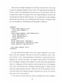
The model file consists of two major sections, one which describes the data model and
one which describes the navigation model. The data model block consists of section
in which the types of vertices which can exist in the data model are defined and a
2
The parser chosen for the DataLink Server is the Apache Xerces XML parser. This parser
was chosen because it adheres to the standard XML specifications issued by the World Wide Web
Consortium (W3C, <http://www.w3.org/>). It is available in both C++ and Java, which makes
porting applications to different language environments easier. Also, it is free and open source.
Xerces distributions and documentation are available for download from the Apache XML Project
website, <http: //xml . apache
3
. org/>.
See XML Schema [Sperberg-McQueen and Thomson, 2002],
Schema\#dev>
4See [The World Wide Web Consortium, 2002a]
46
<http: //www.w3.org/XML/
section which describes how instances of these vertex types are connected together
to construct a model of the physical data. The navigation model block contains
definitions of all the navigation vertices in the navigation model and a specification
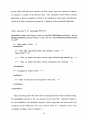
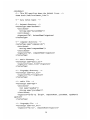
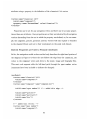
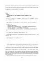
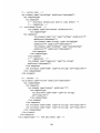
of how all of these vertices are connected. A skeleton of the model file looks like:
<?xml version="1.0" encoding="UTF-8"?>
<modelDefs xmlns:xsi="http://www.w3.org/2001/XMLSchema-instance" xsi:no
NamespaceSchemaLocation="http://city. lcs . mit . edu:8080/data2/models/mode
ls .xsd">
<!-- data model block: -- >
<dataModel>
<!-- This URI specifies where the dataset lives: -- >
<home href="/"/>
<!--
This is where the data vertex type definitions should go. -- >
<!--
This is where the data vertex instances are created. -- >
</dataModel>
<!-- navigation model block: -- >
<navModel>
<!-- Here we define the navigation vertices. -- >
</navModel>
</modelDefs>
This code listing shows the where the two principal blocks of the model file belong.
The modelDef s element is the root element of the model file. Contained within it
are the dataModel and navModel elements, which encapsulate the data model and
navigation model definitions (the term element refers to a construct of the form
<element>element data</element>).
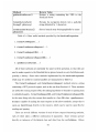
47
Character
&
Use
GET request URLs
GET request URLs
delimits history elements in
DataLink Server requests
Restricted From
navigation vertex names and attribute names
navigation vertex names and attribute names
navigation vertex names
Table 3.1: Reserved characters
3.2.1
An XML Schema is Used For Validation
In the previous example the modelDefs element references an XML schema file,
<http: //city.lcs.mit .edu:8080/data2/models/models .xsd>, which encodes the
definition of the model file format. When the model file is parsed, this schema is used
to check and report errors in the model file's structure and syntax. To ensure that
errors are properly reported during parsing, a reference to this schema should be
included in every model file. A complete listing of model file schema is located in
Appendix B.
3.2.2
Reserved Characters
In general, vertex and attribute names in the model file can contain any character,
including spaces. Some of the special characters used in requests to the DataLink
Server will cause problems if they are used in attribute or vertex names. Table 3.1
lists these characters and summarizes the contexts in which they are reserved.
3.3
Creating a Data Model
This section describes how to model a hierarchical dataset. The example datasets in
this document will be directory hierarchies because the current implementation of the
DataModel class is geared towards modeling directiories. This is a reflection of the
first target dataset of the DataLink Server, the City Scanning Project Dataset, which
is kept on disk in an elaborate directory structure. It should be noted, however, that
the data model is merely an abstraction and that, although the software implementing
48
this abstraction is tailored to modeling directory trees, it would be easy to extend the
data model to provide an interface to any hierarchical data storage system, such as a
database. With that in mind, it's time to being learning how to write a data model.
3.3.1
Data Vertex Type Definitions
Before describing how the the various elements of the data hierarchy are related, it is
first necessary to define all of the different types of data that might be found in the
dataset. As mentioned earlier, this is accomplished with data vertex type definitions,
which have the form:
<vertexType name="data vertex type name">
<!-- Attribute definitions go here: -- >
<attributes>
<!-- integer attribute definitions -- >
<!-- string attribute definitions -- >
<!-- state attribute definitions -- >
</attributes>
<!-- data signatures go in this section -- >
</vertexType>
As this outline shows, a data vertex may contain attribute definitions of three
types, integer attributes, string attributes and state attributes and one or more signature definitions, which tell the DataLink Server how to recognize a datum of this
data type. A data vertex type element can have zero or more attribute definitions
of each of the different attribute types, but the attributes must appear in the same
order they are listed in the vertexType outline, above. That is to say, all the integer
attribute definitions must appear first, the string attributes must appear next, and
the state attribute definitions must be last. This is an artifact of the XML schema
language that is used to define the model document type, which has no construct for
unordered element groupings in which each element of the group may appear more
than once. This restriction is not terribly inconvenient as long as one remembers
49
it when writing model files. In point of fact, this rule carries throughout any XML
document; the elements must appear in a fixed order.
Attribute Definitions
There are two components to every attribute construct: a type declaration and a
name. In essence, attributes are declared in the same way as variables are in any
programming language. Attribute names can consist of any character sequence that
does not include the & or = characters. In addition, attribute names cannot be one
of the three keywords which are used in requests to the DataLink Server: view,
resource and history.
Integer Attributes
True to their name, integer attributes can hold any integer
value. Integer attribute definitions have the form:
<int name="attributeName"/>
String Attributes
The value of a string attribute can be a character sequence of
any length. String attribute definitions look like:
<string name="attributeName"/>
State Attributes
State attributes are a little more complicated than string and
integer attributes. State attribute definitions look like:
<stateVar name="attributeName">
<!-- abstract states: -- >
<state name="abstract
<signature>state 1
</state>
<state name="abstract
<signature>state 2
<signature>state 2
</state>
</stateVar>
state name 1">
signature</signature>
state name 2">
signature 1</signature>
signature 2</signature>
50
A state attribute can assume any one of a discrete set of abstract states. The
abstract states are defined by <state> elements inserted within the body of the
state attribute definition. Every abstract state declaration must include at least one
<signature>.
A signature is a character pattern that the data link server uses
to identify items in the physical data. A signature is a pattern which matches a
filename, or part of a filename, in the case of state attributes. These state signatures
are basically keywords used by the data layer to determine the abstract state of state
attributes from properties of the physical data. If the value of a state attribute
extracted from a filename matches a particular signature of abstract state a, then the
data layer knows that the abstract state of the attribute is a. To see how this works,
let's examine an example from the City dataset.
Recall from Section 1.1.1 that after a City Scanning node is acquired, it enters
a pipeline of post-processing stages. Each of these stages improves the position and
orientation information associated with each image in the node and outputs a new,
refined set of camera files for those images. The camera files for each post-processing
stage are stored in a directory named after that stage, such as initial, mosaic etc.
A state attribute of the pose-ref inement data vertex type, which represents one of
these pose directories, is used to make the data's state of post-processing refinement
a navigable property:
<vertexType name="pose-refinement">
<attributes>
<stateVar name="refinement">
<state name=" initial"><signature>initial</signature></state>
<state name="mosaiced"><signature>mosaic</signature></state>
<state name="rotated"><signature>auto-rot</signature></state>
<state name="translated">
<!-- signatures searched in the order listed here: -- >
<signature>all-trans</signature>
<signature>trans-set4</signature>
</state>
</stateVar>
</attributes>
<signature>"%t", refinement</signature>
</vertexType>
51
As you can see, the refinement attribute has four abstract states, initial,
mosaiced, rotated and translated, representing the four possible states of postprocessing refinement. These abstract state names are not identical to the names of
the pose refinement directories from which they get their values, initial, mosaic,
auto-rot, all-trans and trans-set4, but the <signature> declarations map the
abstract states to the appropriate directory names.
The precise definition of this
mapping is is given by the pose-ref inement vertex's signature, <signature>"%t",
refinement</signature>. Make note that the vertex's signature is different thing
than state attribute signatures. In this example, the vertex signature is a pattern
specifier which says that a pose-ref inement directory's name is equal to the value of
the state attribute refinement. Whatever state signature this value matches determines the abstract state of the refinement attribute. The next section will explain
this mechanism in detail, but the important thing to glean from this discussion is
that, according to the above vertex definition, when the refinement attribute has
the value auto-rot, the DataLink Server recognizes rotation as the abstract state
of the refinement attribute, and similarly for the other states and state signatures.
Notice that the translated state has two signatures, all-trans and trans-set4.
This is because the City scanning dataset contains data from multiple runs of the postprocessing algorithms. 5 Instead of overwriting the old data each time the algorithms
are run, the author of the new data may sometimes rename the old directories for
safe keeping.
As a byproduct of this practice, there are some nodes in the City
dataset whose translated camera files are stored in alltrans directories, some whose
translated data are stored in trans-set4 directories and some nodes that have both
all-trans and trans-set4 directories.
In general, when the DataLink Server is searching for data with an abstract state
that has more than one signature, it gives precedence to data with the signature that
appears first in the <state> declaration, so, for nodes with both alltrans and
5
As new data is acquired, the post-processing pipeline is often reapplied to the entire dataset
in order to take advantage of any new global features, such as vanishing points and baselines, that
have been discovered in the new nodes.
52
Example
unbound
extracted from auto-rot datum or
requesting auto-rot data
in request for rotated data
Abstract State
null
rotated
Literal State
null
auto-rot
rotated
null
Table 3.2: Valid state pairings listed by example
trans-set4 directories, the DataLink Server will return the contents of the all-trans
directory when it receives a request for camera files in the translated abstract state of
pose refinement. It is possible to make requests to the DataLink Server which override
this behavior in order to obtain camera files from only the trans-set4 directories or
vice versa.
State Attributes Have Abstract and Literal Values
State attributes can
hold two types of values simultaneously, an abstract state and a literal state. The
literal state of a state attribute is the particular state signature that it is bound to.
When state attributes are extracted from physical data they will have both a literal
state, which was obtained from the data itself, and a corresponding abstract state.
When making requests to the DataLink Server, the client may only be interested in
the abstract state of the data, so, in this case, it will make a request with only the
abstract state of the state attribute defined. In other cases, such as when the client
wants to make a request for only the trans-set4 data, it may make a request with
the literal state of the refinement attribute specified. Table 3.2 lists some examples
using the refinement attribute which illustrate each of the possible value pairings a
state attribute may assume.
Data Vertex Type Signatures Define the Mapping of Attributes and Data
Data vertex type signatures define the mapping between attributes and physical data
and, conversely, tell the DataLink Server how to derive attribute values from an
instance of a data type in the dataset. This example vertex from the City Scanning
Project Dataset should help to illustrate how signatures work:
53
<vertexType name="image">
<attributes>
<int name="imgId"/>
</attributes>
<signature>"%.4d.rgb", imgId</signature>
</vertexType>
This sample is the data vertex type definition for an image in the City dataset.
Each node in the City dataset consists of a collection of numbered .rgb images with
filenames of the format 0000.rgb, 0001.rgb etc. The four-digit number in the name
of each image is the image's ID, which is captured by the imgId attribute of the image
data vertex type. The signature that maps the four digit image ID in the image's
filename to the imgId attribute is simply a C-style string format expression with the
token %. 4d in the place of the image ID number.' The signature expression indicates
that the value of this token is equal to the value of the imgId integer attribute.
String format expressions like these are all that is necessary to extract the salient
attribute values from file and directory names in a directory hierarchy. Although it
was not necessary for the City Scanning Project Dataset, a similar mechanism could
be added to the data model for extracting attribute values from data actually stored
within the data files themselves, and it would not be much of a stretch to add a
parallel construct for obtaining attribute values from database keys.
Table 3.3 lists the tokens that can be used in signature expressions. Most of these
are identical to their counterparts in C. In addition I have added two new tokens, t
and T, for formatting state attributes. 7
It is not uncommon to find datasets with inconsistent naming schemes. To combat
this problem, the DataLink Server supports the capability to define multiple signatures per data vertex type. As is the case for state signatures, the DataLink Server
6
This discussion assumes the reader is familiar with the syntax of C string format expressions.
However, for a reference or a quick review, look in any C/C++ guidebook. I recommend C++: The
Complete Reference [Schildt, 1995].
7The current implementation of the DataLink Server does not support the full gamut of format
tokens that C programmers may know about (there was no need for floating point attributes in the
City dataset), but the string format expression code is modular enough that format tokens for new
data types can be added without tribulation. Other than the floating point tokens, most of the other
C format tokens can be subsumed by the d token, anyway. In addition, there is no support for the
hexidecimal format modifier, #, and I do not foresee there ever being a need for the * modifier.
54
Format Token
Attribute Type
int
%d
string
stateVar (abstract state)
stateVar (literal state)
%s
%T
%t
Table 3.3: String format expression tokens used by the Dat aLink Server
DataModel
<name='DATASET",
type="dataset">
datsetName
<name=COMPOSER",
type="composer-dIr">
composerName
<name="MUSICFILES,
type="music_dir">
<name=OPIECES,
type='mp3">
<name='BIO
DIR',
type = 'bio_dir">
<name="BIOGRAPHY",
type="bio-doc">
<name="PORTArTr,
type="portafltmg'>
opusNum
pleceName
Figure 3-1: Data model of a classical music library
will give preference to the data vertex type signature which appears first in the body
of a data vertex type definition.
3.3.2
Declaring Data Vertex Instances
Now that that the tools for describing the data have been garnered, it's time to learn
how to declare instances of these data types and connect them together to form the
data model graph. An example is the best way to demonstrate how to do this, so
let's begin by seeing how we would create a data model for the classical music dataset
from Chapter 2 (A diagram of this dataset is duplicated for convenience in Figure 31): First, let us use the information from the previous section to create an explicit
definition of the data itself:
55
<dataModel>
<!-- This URI specifies where the dataset lives:
<home href="/usr/local/musicjlibs"/>
<!-- data vertex types:
-- >
<!-- dataset directory:
-- >
-- >
<vertexType name="dataset">
<attributes>
<string name="datasetName"/>
</attributes>
<signature>"%s",
</vertexType>
datasetName</signature>
<!-- composer directory: -- >
<vertexType name="composer-dir">
<attributes>
<string name="composerName"/>
</attributes>
<signature>"%s", composerName</signature>
</vertexType>
<!-- music directory: -- >
<vertexType name="musicdir">
<signature>"audio-files"</signature>
</vertexType>
<!-- biography directory: -- >
<vertexType name="bio-dir">
<signature>"bio"</signature>
</vertexType>
<!--
audio file: -- >
<vertexType name="mp3">
<attributes>
<int name="opusNum"/>
<string name="pieceName"/>
</attributes>
<signature>"Xs-%s-op. %d.mp3", composerName,
ignature>
</vertexType>
<!-- biography file: -- >
<vertexType name="biodoc">
<signature>"%s.txt", composerName</signature>
56
pieceName,
opusNum</s
</vertexType>
<!-- picture of composer: -- >
<vertexType name="protrait_img">
<signature>"Xs . jpg", composerName</signature>
</vertexType>
<!-- This is where the data vertex declarations will go. -- >
</dataModel>
This data model says that our music library is contained within a directory
with some name like, "classical" which should be stored in the datasetName attribute.
Inside this directory are some subdirectories such as Johannes Brahms,
Modest Mussorgsky etc., which are named after the composers in the library. In
each composer directory there are two subdirectories with fixed names: audio-f iles
and bio. Each bio directory contains a biography file and a portrait of the composer, and held within each audio-f iles directory are the pieces written by composer, whose filename is constructed from the composer's name followed by the title of
the work and the opus number (i.e. Johannes Brahms-Sonata for Clarinet and
Piano no.
1-op.
120 .mp3). Notice that attributes are declared at the highest level
of the hierarchy in which they appear, and declarations for them are omitted from
vertex type definitions for data that lie beneath this node in the data hierarchy. This
is because when instances of these data vertex types are connected together to form
a graph, these attributes will be inherited. Let's do that now:
<dataModel>
<!-- data vertex declations:
-- >
<vertex name="DATASET" type="dataset"/>
<vertex name="COMPOSER" type="composer-dir">
<parent name="DATASET"/>
</vertex>
57
<vertex name="MUSICFILES" type="musicdir">
<parent name="COMPOSER"/>
</vertex>
<vertex name="BIODIR" type="bio_dir">
<parent name="COMPOSER"/>
</vertex>
<vertex name="PIECES">
<parent name="MUSIC_FILES"/>
</vertex>
<vertex name="BIOGRAPHY">
<parent name="BIO_DIR"/>
</vertex>
<vertex name="PORTRAIT">
<parent name="BIO_DIR"/>
</vertex>
</dataModel>
See how the parent command has been used to specify the edges in the data
model? That's all there is to it. The structure of the vertex element has left open the
possibility of vertices having more than one parent. This is not currently supported
by the DataLink Server because allowing only one parent per vertex greatly simplifies
the computational complexity of the algorithms used in the DataLink Server's implementation (see Chapter 5). Room has been left in the DataLink Server code for the
possibility of this extension, however.
3.4
Writing a Model To Direct Navigation
Now that you know how describing the data is accomplished you can learn how to
make it navigable. This is the purpose of the navigation model block of the model
file, which describes the interconnections between a network of navigation vertices.
The basic outline of a navigation model looks like this:
<navModel>
<!--
navigation vertex declarations go here.
<root name="name of root navigation vertex"/>
58
-- >
Navigation Model
<name="classical ib",
type="dataset">
<name="opus number"> +-+ <name="composer",
type="composer_dir">
<name="pleces",
<name="portrat,
<name="blo",
type="mp3">
type="portalt-Img">
type="blo-doc">
Figure 3-2: Navigation model of the classical music library
</navModel>
3.4.1
Defining Navigation Vertices
Enumerating a list of all the features involved in creating a navigation model would
be tedious to read and far less trenchant than a series of demonstrative examples, so,
in that light, we will continue this discussion of navigation models by building one for
the classical music library. The basic structure of the navigation model we will build
is shown in Figure 3-2. After detailing how this navigation model is put together,
this section will show how additional parameters of navigation vertices can be used
to fine tune the DataLink Server's exhibition of this model.
The best way to design a navigation model is from the bottom up starting with
vertices for the files to make available:
<navModel>
<vertex name="pieces" type="mp3"/>
<vertex name="portait" type="portait-img"/>
<vertex name="bio" type="bio-doc"/>
</navModel>
59
This exposes the images, biography text documents and audio files to the navigation layer by assigning navigation vertices to them. The type argument grounds each
of these vertices to the appropriate data vertex type in the data model. When the
navigation layer explores a navigation vertex with a type declaration, it knows to ask
the data layer for instances of that data type. As it stands, however, this navigation
model doesn't provide any way of reaching this data because no navigation paths
have been specified yet. The following code listing adds a simple one:
<navModel>
<vertex name="classical lib">
<child name="composer"/>
</vertex>
<vertex name="composer" type="composerdir">
<child name="pieces"/>
<child name="portrait"/>
<child name="bio"/>
</vertex>
<vertex name="pieces" type="mp3"/>
<vertex name="portait" type=I"portaitimg" />
<vertex name="bio" type="bio...doc"/>
<root name="classical lib"/>
</navModel>
The path described here begins at the vertex named classical lib, as specified by the root command. From here the user will be allowed to select a composer directory to view. The DataLink Server will present a composer link for every
composer-dir it finds in the dataset. The default content handler of the DataLink
Server will display a listing for the classical lib vertex that looks something like
Figure 3-3. Clicking on one of the composers' names will take the user to the composer
vertex where the DataLink Server will display something similar to Figure 3-3 with
sections for pieces, portrait and bio. Observe how the child command is used to
create these edges in the navigation graph by naming the next vertex a user could be
able to get to from a given location.
At this point the reader may have noticed something queer about navigation
60
MEMEL -
Current Path: classical lib
Antonio Vivaldi
George Gershwin
Johannes Brahms
Modest Mussorgsky
Figure 3-3: Listing of the classical lib vertex
model and the output of the DataLink Server for the classical lib vertex. At no
point in the navigation graph was the user given an option to choose the value of the
datasetName attribute, which, according to the data model that was developed in
Section 3.3.2, is necessary to resolve a path to the composer directories. Somehow
the DataLink Server was able to produce results for the composer vertex anyway.
To understand how this happens recall the specification of the navigation layer's
interaction with the data layer. When the navigation layer requests a set of branches
for a data vertex type, it is asking for all sets of attribute bindings which completely
specify a data and are consistent with the set of attribute values determined by the
current path through the navigation hierarchy. When the user first connects to the
system at the classical lib vertex, no attribute values have been accumulated yet,
so any set of attribute bindings that specifies a composer-dir will be returned by the
data layer. The datasetName attribute has a value; it's just been hidden from the
user.
Now, suppose that the directory named classical, which houses the classical
music dataset, shares a parent directory with another dataset, punk-rock. punk-rock
is the home of another music library with roughly the same structure as the classical
dataset. Inside punk-rock are some directories named after punk rock bands which
are equivalent to composer directories in the classical dataset. Now when the user
visits the classical lib vertex the DataLink Server will output a listing like the
one shown in Figure 3-4.
Dead Kennedys et. al. are not the names of classical music composers. In the listing of Figure 3-4 the DataLink Server has branches for the "composer" directories from
61
Current Path: classical lib
Antonio Vivaldi
George Gershwin
Johannes Brahms
Modest Mussorgsky
Dead Kennedys
Rancid
The Exploited
e Rnes
The Sex Pistols
Figure 3-4: Another listing of the classical lib vertex
both datasets. The "classical" branches represent sets of attribute bindings that look
like {datasetName = "classical", composerName = "Johannes Brahms"} and the
"punk" branches have attribute binding sets such as {datasetName = "punk..rock",
composer = "The Clash"}.
Usually this type of behavior is desirable.
For example, if the name of the
composer lib vertex was changed to music lib the output of Figure 3-4 would
be appropriate. Suppose, however, that in this case we only want to make the classical library navigable.' One way of doing this would be to change the signature of the
dataset vertex type to <signature>"classical"</signature>. There are some
cases, however, where there value of an attribute should be fixed for certain parts
of the navigation hierarchy only. One example from the City dataset is a "show all
rotated nodes" vertex, which would be the start of a navigation hierarchy for browsing only nodes that have completed the rotation post-processing phase. This new
hierarchy would be in addition to the regular hierarchies for browsing the nodes in
all post-processing stages and the way to implement it is with properties.
Attribute Values Can Be Fixed Using Properties
A property declaration has two arguments: the name of the attribute to set and the
value to assign it. The following listing shows how to fix the value of the datasetName
8
The music library is to be made available to the employees of the British Consulate, who's
administration does not share the same views of Queen Elizabeth as The Sex Pistols.
62
attribute using a property in the definition of the classical lib vertex:
<vertex name="classical lib">
<child name="composer"/>
<property name="datasetName" value="classical"/>
</vertex>
Properties can be set for any navigation vertex and there can be as many properties as there are attributes. Once properties are set they are inherited by all navigation
vertices descending from the one in which the property was defined, so, for our example, the composer, pieces, portrait and bio vertices will only expand to branches
in the classical library and not to their counterparts in the punk rock dataset.
Derived Properties are Used to Promote Attributes
So far, the navigation model we have scribed only describes the right-hand portion of
the diagram in Figure 3-2 where the user follows the edge from the classical-lib
vertex to the composer vertex and down to the music, image and biography files.
This next code segment adds the left-hand path through the opus number vertex
(comments have been included to indicate the changes):
<navModel>
<vertex name="classical lib">
<child name="composer"/>
</vertex>
<vertex name="composer" type="composerdir">
<child name="opus number"/> <!-- added this edge -- >
<child name="pieces"/>
<child name= "portrait"/>
<child name="bio"/>
</vertex>
<!-- added this vertex: -- >
<vertex name="opus number">
<child name="composer"/>
63
<child name="pieces"/>
<derivedProperty name="opusNum" source="mp3"/>
</vertex>
<vertex name="pieces"
type="mp3"/>
<vertex name="portait" type= "portaitimg"/>
<vertex name="bio" type="biodoc"/>
<root name="classical lib"/>
</navModel>
In this example the <derivedPropery> command has been used to promote the
opusNum attribute to a higher level in the hierarchy. The branches displayed by the
DataLink Server for the opus number vertex when viewed from the classical lib
vertex will be the set of all unique opus numbers that exist in the dataset. The source
argument of the derivedProperty tells the DataLink Server how to determine what
the possible values of the derived property are. In this case the DataLink Server is
instructed to do this by examining all of the mp3 files that are consistent with the
attribute values set by the user's current path through the navigation hierarchy. When
the user is at the classical lib vertex, no attribute values have been accumulated,
so the branches displayed for the opus number vertex are the opus numbers for every
mp3 file in the dataset. When the user is at the composer vertex, composerName has
been bound to a value, so the set of opus number branches includes only the opus
numbers of works by the selected composer.
Attribute Redirection
Attribute redirection can be used to reassign a named value to the name of an attribute for a particular vertex by using a redirect command in the body of a navigation vertex. The redirect command has the syntax:
<redirect source="name of source" destination="name
of destination">
One example of where this is useful is a pair of special navigation vertices which
bring up the baseline files for a particular node in the City dataset. Baseline files
have a signature which looks like:
64
Parameter
supress-incomplete.leaves
merge-duplicates
enumerate-history
Default Value
false
true
true
Table 3.4: Default values of navigation vertex parameters
<signature>"%.4d_%.4d.trans", fromNode, toNode</signature>
Attribute redirection can be used to find the "to" baselines for the currently
selected vertex. The "to" baselines are the baselines which point from the current
node to another node (i.e the baselines for which fromNode is the currently selected
node). To find the "to" baselines for the currently selected vertex, the City dataset
employs a special navigation vertex, to baselines which has the definition:
<vertex name="to baselines" type="baseline-file">
<redirect source="nodeId" destination="fromNode"/>
</vertex>
When the datalink server encounters this vertex, it assigns the value of nodeId (if
any) to fromNode. A similar vertex is used to find the "from" baselines of a node.
Navigation Vertex Parameters
Navigation vertices have a small number of Boolean parameters which affect how
they are handled by the DataLink Server. The names and the default values of these
parameters are summarized in Table 3.4.
The author of a navigation model can
override the default values of these parameters for some vertices by including a param
command in the body of the navigation vertex's definition. The param command has
the syntax:
<param name="parameter-name"
value="true I false "/>
65
supress-incomplete-leaves
The supress-incomplete-leaves parameter is relev-
ent to the opus number navigation vertex that has just been added to the navigation
model. As it stands now, when the user visits this vertex from the classical lib
vertex, the DataLink Server will display branches for every composer in the dataset
that has written a piece with the selected opus number as well as a set of branches
for every audio file in the dataset with the selected opus number. This might be
the behavior intended by the web architect. On the other hand, if the purpose of
the opus number vertex was merely to reverse the order in which the user can select
values for the opus number and composer name attributes then the DataLink Server
shouldn't display audio files when the user is at the opus number vertex unless the
user has arrived there from the composer vertex, and thus, has selected a value for
the composer name attribute.
To force the DataLink Server to take this second
approach the suppress-incomplete-leaves parameter should be set to true for the
opus number vertex as follows:
<vertex name="opus number">
<child name="composer"/>
<child name="pieces"/>
<derivedProperty name="opusNum" source="mp3"/>
<param name="supress-incompleteleaves" value="true"/>
</vertex>
When the suppress-incomplete-leaves parameter is set the DataLink Server
will supress the display of branches for leaf navigation vertices whose inherited attribute values have not been completely specified by the current navigation path.
Therefore, with the suppress-incomplete-leaves parameter set, when the DataLink
Server is at the opus number vertex it will not display branches for audio files unless
it knows values for both the datasetName and composerName attributes.
merge-duplicates
Sometimes the order of two attributes can be switched by some
means other than a derived property. One example occurs in the City dataset for
the attributes for image resolution and state of post-processing refinement. These
66
attributes derive their values from the names of directories in the City dataset. In
the physical hierarchy of the City dataset the resolution directories are the parents
of the post-processing directories. The navigation model for the City dataset allows
the selection of these attributes to be reversed by cross-referencing the navigation
vertices associated with them:
<navModel>
<vertex name="pose refinement" type="pose _refinement">
<child name="resolution"/>
</vertex>
<vertex name=1"resolution" type="resolution">
<child name="pose refinement"/>
</vertex>
</navModel>
In this case, when the user chooses a state of post-processing refinement first, the
system should not behave as if a value for the refinement attribute has also been
selected. The DataLink Server recognizes this case when it finds two branches with
identical names but different sets of attribute bindings. For example, if the user made
a selection for a state of post-processing refinement before choosing a node ID the
system would find a whole bunch of branches named "half' for the image resolution
attribute. The DataLink Server knows better than to provide selections for each of
these branches. The DataLink Server would recognize that some of these like-named
branches have different values for the node ID attribute, triggering the branch merging
process which unifies all of the branches with similar names into one.
67
When two branches are merged, they are generalized. This means that all of the
attribute bindings for attributes that were not set by the user via navigation which do
not belong to the data vertex type (if any) of the navigation vertex of the branches
are annulled.
Thus, if the DataLink Server identified these two branches for the
resolution vertex: {nodeId = 0, refinement = "rotated", resolution = "half "}
and {nodeId = 1, refinement = "rotated", resolution = "half "} when the user
had just made a selection for refinement, the DataLink Server would forward only
one branch to the presentation layer. This branch would have the following set of
generalized attribute bindings: {ref inement = "rotated", resolution = "half "}.
The algorithm that performs branch merging and generalization is O(n), where
n is the number of branches before merging, so there is a small cost associated with
merging when the number of branches is large. When it is known that duplicate
branches can never occur for a particular navigation vertex, the merge-duplicates
parameter can be set to false to disable the merging process for that vertex and improve the performance of the DataLink Server. The node vertex of the City dataset's
navigation model is a good example of this because every node directory is identified
by a unique ID number, and, therefore, there can never be duplicate branches for the
node vertex.
enumerate-history
In addition to the branches for each child of the selected
vertex, the DataLink Server also returns sibling braches for all of the vertices in
the history of the current navigation path. These can be formatted by using the
BranchHistoryScripter tool in the DataLink Server API to create context menus
which allow the user to jump back to earlier points in the navigation path, or to
quickly make an alternate selection for a previously visited vertex. Enumeration for
individual vertices can be turned off by setting the enumerate-history parameter to
false. This can be used to reduce computation or to prevent the display of menus for
vertices which have may have a very large number of branches.
68
Formatting Rules for Branches and Branch Classes
The DataLink Server provides a couple of formatting options for branch names and
branch class names. A branch class is the set of all branches belonging to a particular
navigation vertex. In the default content handler view, the branch class name is used
for the heading placed above the branch listing for a particular navigation vertex. As
you can see from Figures 3-3 and 3-4, the default name for each branch class is simply
the name of the corresponding navigation vertex.
A better branch class name can be provided for each navigation vertex by adding a
branchClassName declaration to the body of the navigation vertex definition. There
is a similar command, branchName which performs the same function for the names
of branches. Any valid string format expression of the same form as a data vertex
type signature expression can be used for a branch name or a branch class name.
The following code example shows how to improve the formatting of the composer
vertex:
<modelDefs xmlns: xsi="http: //www .w3. org/2001/XMLSchema-instance" xsi:no
NamespaceSchemaLocation="http://city. ics.mit. edu: 8080/data2/models/mode
is.xsd">
<dataModel>
<!-- composer directory: -- >
<vertexType name="composerdir">
<attributes>
<string name="firstName"/>
<string name="middieName"/>
<string name="surname"/>
</attributes>
<signature>" 0 s %s %s", firstName, middleName, surname</signature>
<signature>"%s %s", firstName, surname</signature>
</vertexType>
</dataModel>
69
<navModel>
<vertex name="composer" type="composer.dir">
<child name="opus number"/>
<child name="pieces"/>
<child name="portrait"/>
<child name="bio"/>
<branchName>"Xs, %s", surname, firstName</branchName>
<branchClassName>"Composers"</branchClassName>
</vertex>
</navModel>
</modelDefs>
Now the heading for composer branches will be "Composers" and each composer
branch itself will have the form "Brahms, Johannes".
Notice that to do this some
new attributes, firstName, middleName and surname had to be created, and the
signature for the compser-dir had to be modified to extract the values for these
attributes.
In this listing I've only shown the changes relevant to this discussion
on name formatting, but, clearly other vertices in the navigation and data models
would have to be augmented with the new attributes, as well. The main thing to
take away from this example, however, is how the two branch formatting commands,
branchName and branchClassName are used.
Assigning Content Handlers to Navigation Vertices
To assign a custom content handler to a navigation vertex the contentHandler command is used. Here is an example of this command's usage:
<vertex name="composer"
type="composer-dir">
<child name="opus number"/>
<child name="pieces"/>
<child name="ortrait"/>
70
<child name="bio"/>
<branchName>"%s, %s", surname, firstName</branchName>
<branchClassName>"Composers"</branchClassName>
<contentHandler>/composer. jsp</contentHandler>
</vertex>
The contentHandler commands specifies a URL to the content hander for the
vertex. This URL must begin with a forward slash, which specifies a URL relative to
the home directory of the webapp where the DataLink Server is deployed.
3.5
Chapter Summary
That's pretty much all there is to the model file format.
Now that you know how
to use the XML-based modeling language to describe the organization of a physical
dataset and the attributes of the data which should be navigable by writing a data
model definition, as well as how to describe the navigable hierarchies the behavior
of the navigation layer by defining a navigation model, you have mastered almost all
you need to know to begin deploying powerful web interfaces to hierarchical datasets
using the DataLink Server. The next skill to acquire is the ability to write content
handlers to provide a clean, modular custum fagade to the web interface provided by
the DataLink Server. This will be the subject of the next chapter.
71
72
Chapter 4
Content Handlers
This chapter describes the API tools the DataLink Server package provides for writing content handlers. These tools include the DataLinkDispatcher, which allows
a programmer to make requests to the DataLinkServlet for a particular branch or
a resource with a given set of attribute values, and the BranchHistoryScripter,
which allows a programmer to insert interactive menus to give the user some sense
of the multidimensionality of the data space. This chapter also discusses the data
structures which are used by content handlers and the DataLinkServlet to exchange
information and describes the format of requests made to the DataLinkServlet.
4.1
Content Handlers Are JSPs, Servlets or HTML
Documents
Dynamic content handlers can be constructed using Java Server Pages or Java servlets.
In order to have access to the DataLink Server API, content handlers must reference
the DataLink Server package by including the line:
import datalink.*;
This gives the content handlers access to the Java classes that are used to communicate with the DataLinkServlet, format branches and create context menus, as
73
well as the data structures for storing branches and branch classes. There are also
some data structures for attributes and their values which are located in the package
datlink.model.data.attribute
There is no reason why HTML documents, or anything that can be referenced
on the world-wide-web via a URL cannot be used for content handlers, but any
components other than servlets and JSPs cannot access the Java-based DataLink
Server API, so these alternative content handlers would only be able to display content
that doesn't make use of any of the data forwarded by the DataLinkServlet.
4.2
The Format of DataLinkServlet Requests
Before we can begin discussing the interaction between content handlers and the
DataLinkServlet it is important to make note of a few of the essential pieces of a
DataLinkServlet request. Requests can be made to the DataLinkServlet using the
GET or POST protocols. A request in the GET format has the general form outlined
below: 1
http://city.lcs.mit.edu:8080/data2/DataLink?view=node&dataset=all-nodes
-fixed&nodeId=75&history=dataset :allnodes
The first parameter in this request URL, view specifies the name of the vertex
to select. The history parameter specifies the list of vertices that have been visited
along the current navigation path delimited by the : character, not including the
currently selected vertex, which, in this case, is node. The rest of the parameters are
the names and values of attributes.
The client can specify additional parameters in a DataLink Server request using
the same name=value construct that is illustrated in this example. The DataLink
'The name of the DataLinkServlet has been been shortened in this URL to DataLink using a
customization parameter of the webapp which deploys the DataLink Server. The reader unfamiliar
with JSP and Java servlets might not know that the standard API for these tools allows the web
author to create custom URLs for serviets and JSP deployed in a webapp, as has been done here
for the DataLinkServlet.
74
Server treats any additional arguments to the request which do not correspond to
attribute names as additional parameters for the content handler of the selected
vertex and passes them on to the content handler, without interference.
The author of a content handler should never have to write a request like this by
hand. The DataLinkDispatcher provides an API for formatting these request automatically, given an appropriate set of arguments, and this chapter shall not make a
mention of the request format again, but before proceeding any further it is necessary
for the reader to understand the operation of the history parameter because it is
crucial in maintaining smooth navigation through the navigation hierarchies.
4.2.1
The history Parameter
The value of the history parameter is an ordered list of the navigation vertices that
have been visited along the current navigation path. The primary reason that the
DataLink Server needs to maintain a history is to ensure that a user can never visit
the same navigation vertex twice along a single path through the navigation hierarchy
when the navigation model contains cycles. Cycles are usually introduced into the
navigation model by cross-references between navigation vertices which are used to
make it possible for the user to invert the order in which a pair of attribute value
The function of the history is clearly a pretty important one, which might leave
the reader asking why it is passed around as a parameter in DataLinkServlet request
and not maintained somewhere in the internal state of the DataLink Server or in a
Java Bean. The reason is that it is important for the DataLink Server to maintain
a stateless architecture because it is implemented as a Java servlet. Well designed
Java servlets should not maintain any state because the length of their lifecycle is not
guaranteed. The servlet container can start and stop servlets at will, as long as they
are not currently handling a request, in an effort maintain a good load balance on
the host machine. This means that subsequent requests to the DataLink Server may
be handled by different run-time instances of the DataLinkServlet class, and consequently, it is dangerous to try and maintain an internal state in the DataLinkServlet.
For a similar reason, it is also not a good idea to maintain state information, like the
75
navigation history, within Java Beans. 2
Another reason that the history is passed as an argument is that it serves as an implicit request for history enumeration, which can be used to make context navigation
menus like the ones that are created by the BranchHistoryScripter. Section 4.5 in
this chapter will expound the details of this use of the history further.
It is not necessary for the content handler developer to understand the format of the history parameter or how it is maintained, since this is the job of the
DataLinkDispatcher.
The developer of content handlers just needs to be aware
of the history's purpose in order to understand when to use DataLinkDispatcher
routines that invoke it and when it is safe to use the ones that do not.
4.3
Data Structures for Content Handlers
The chief purpose of content handles is to format the data served by the DataLinkServlet
in a useful and pleasing way. Therefore, to write content handlers one needs to be
familiar with the data structures that are used by the DataLink Server to encapsulate
the data it communicates to them. This section outlines all of these important data
structures briefly.
4.3.1
The DataLinkServlet Communicates to Content Handlers Using the curPathBean
All of the information about branches and navigation vertices that the DataLinkServlet provides for content handlers is communicated using a Java Bean called the
curPathBean. The DataLinkServlet passes this bean to the content handler of a
navigation vertex when that vertex is selected. This curPathBean is an instance
of the NavPathBean class. This class has a number of routines for use in content
handlers which can be used to obtain information about the current navigation path
2
Any reference book on JSP and Java Servlet technology, such as Proffesional JSP
[Brown et al., 2000], should be able to provide a more thorough treatment about the life cycles
of servlets and Java Beans.
76
Method
Return Value
getCurVtxAttrs 0
An AttributeMapBean containing the attributes
bindings of the current navigation path
getHistory()
A String[
retrieveBranchClass (
"nav vertex")
The BranchClass for "nav vertex"
branchClasses 0
An Iterator containing the names of all the children
of the selected vertex for which the DataLinkServlet
has found branches
containing the current navigation history
Table 4.1: NavPathBean routines for use in content handlers
and the available navigation options. Table 4.1 summarizes these methods. As you
can see from Table 4.1, the curPathBean uses a number of additional data structures
for encapsulating the information it holds about branches and attributes.
4.3.2
Data Structures for Attributes
Table 4.2 lists the three map classes that are useful in content handlers for storing
sets of attribute name/value pairs. All of these maps have the same basic interface which includes a get ("name") method for retrieving a named attribute value,
and a number of put("name", V) methods for storing the value of an attribute.
NamedValueMap and SimpleNamedValue map are essentially the same except that
SimpleNamedValueMap has a simplified API that makes it compatible with Java 1.0.
SimpleNamedValueMap is the storage class of choice for use in Java applets embedded
in content handlers because its JDK 1.0 compatibility will ensure that the applet can
run in older browsers.
The two named value map classes are utility classes for passing arguments to
the DataLinkDispatcher to form requests to the DataLink Server. They should be
used whenever the content handler needs to make a request using attribute values
that were not provided as part of the current navigation path or a branch by the
DataLinkServlet. If the navigation model for the dataset is designed properly, there
should almost never be a need to do this in the body of a content handler because the
77
Map
AttributeMapBean
Values Type
AttributeBean
Usage
Used to store attributes bindings provided by the DataLinkServlet
NamedValueMap
String
Used to form custom queries (JDK 1.2)
SimpleNamedValueMap
String
Used to form custom queries (JDK 1.0)
Table 4.2: Map data structures for holding attribute sets
web architect can usually supply all of the data a content handler will need by making
edges to the appropriate navigation vertices. The content handler can then access
the data using the routines from the DataLinkDispatcher interface that can operate
directly on the branches produced for these vertices. The two primary exceptions
occur when the value of an attribute comes from a cache or when the request is made
from within a Java applet, which cannot have direct access to the curPathBean.
The AttributeMapBean is the representation used by the curPathBean to store
attribute bindings forwarded by the DataLinkServlet. Attributes are stored in an
AttributeMapBean in bean form as instances of the AttributeBean class. This class
has a very simple interface which includes a getName () and a getValue method.
State attributes are stored as a subclass of AttributeBean, StateAttributeBean,
which has an additional method, getState O, for retrieving the abstract state of a
state attribute.
A Word About State Attribute Values
All of the map classes for storing attributes can work with attribute values represented
as strings. Attributes values of any type can be represented as strings, but there are
some special considerations for state attribute values in string form. Recall from
Section 3.3.1 that state attributes can have an abstract state with no literal state or
both an abstract state and a literal state. When a state attribute has a literal state,
the string version of its value is simply the literal state it is in (i.e. "auto-rot"). When
a state attribute has only an abstract state its string value is the name of the abstract
state prefixed with a ! character, as in "!translated". This reflects the way state
78
attributes values are passed in a query string to the DataLink Server. The getValue ()
method of the StateAttributeBean class will output string representations of state
attribute values according to this convention.
4.3.3
Data Structures for Branches
The DataLinkServlet bundles all of the branches for a single navigation vertex into
a BranchClass class. In addition to storing the branches themselves, a BranchClass
stores some data which is shared by all of the branches in the class. This includes the
name of the source navigation vertex and a flag which specifies whether the branches
correspond to resources (physical files). Table 4.3 lists the methods of BranchClass
which are of interest to authors of content handlers.
The branches themselves are represented by instances of the Branch class. The
methods this class provides for getting at the data are given in Table 4.4. In an
effort to reduce redundancy, the DataLinkServlet returns all of the attribute bindings of the current navigation path, which are shared by all of the branches, in the
curPathBean. Only the attribute bindings which are specific to individual branches
are stored in the branches themselves. Thus, the complete set of attributes for a
given branch is a union of the current path's attributes and the attributes stored in
the Branch class for that branch:
curPathBean.getCurVtxAttrs 0
4.4
U branch.getAttributes
0
The DataLinkDispat cher Is Used to Format Requests to the DataLink Server
Now that the details of the data structures for storing attributes and branches have
been articulated, the use of the DataLinkDispatcher can be investigated.
The
DataLinkDispatcher implements several different versions of these five methods for
interfacing with the DataLinkServlet:
79
Method
getName 0
Return Value
The name of this branch class, as specified in the navigation
model
getNavVtxName()
The name of the navigation vertex corresponding to this
branch class
getBranches 0
A Branch [I of all of the branches in this class
isResource 0
true if the branches are resources (leaf vertices); false if
they are navigation vertices
Table 4.3: BranchClass routines for use in content handlers
Method
getBranchName ()
Return Value
The formatted name of this branch, as specified in the
navigation model
getAttributes()
An AttributeMapBean containing the attribute bindings
of this branch
getLastModified(
The timestamp of the branch in milliseconds, if the
branch is for a navigation vertex that is associated with
a data type; -1 if the source vertex is purely navigational
getSize 0
If this branch is associated with a physical datum, this
method returns its size in bytes; it returns 0 if the associated navigation vertex is purely navigational
Table 4.4: Branch methods for content handlers
80
Method
getDataLinkServer()
Return Value
Returns a string containing the URL to the
DataLink Server
formatHistoryPath(
String[] pHistory)
Formats the navigation history into a path-like
string delimited by / characters
sortBranches (Branch [
pBranches)
Sorts a branch array lexicographically by name
Table 4.5: Other useful methods provided by the DataLinkDispatcher
1. formatViewRequest(... )
2. formatViewResourceRequest(...)
3. formatViewRequestURL(... )
4. formatViewResourceRequestURL(...)
5. openResourceStream(...)
All of these methods are essentially the same in their operation, in that they are
used to make requests to the DataLink Server given a branch or a set of attributes and,
possibly, a history. Some other methods implemented by the DataLinkDispatcher
which may be useful for content handlers are summarized in Table 4.5.
The formatViewRequest and formatResourceRequest methods return a string
containing a GET protocol request, such as the one from Section 4.2. These methods
are useful for creating request URLs for making hyperlinks to branches or passing data
to embedded applets. f ormatViewRequestURL and f ormatViewResourceRequestURL
do the same thing only they output their results in a Java URL class. openResourceStream is capable of making the same requests as the above methods, except that it
opens an InputStream directly to the resource, which can be used to open files for
reading and parsing.
There are several different versions of each of these request formatting methods,
each of which takes a different combination of arguments. Some versions operate
directly on instances of the Branch class and data from the curPathBean. Others
81
enable the programmer to use the attribute map data structures from Section 4.3.2
to make requests using an arbitrary set of attribute bindings. To go into the details
of each of these variations would be overly fastidious. However, the interested reader
can examine the exhaustive listing of the methods in the DataLinkDispater API
that is located in Appendix A.
4.4.1
View Requests vs. View Resource Requests
In and of itself, the formatViewRequest method provides all of the functionality
needed to make requests to the DataLink Server. The other methods exist primarily
for convenience and simply incorporate a few other tasks that are commonly associated with making requests to the DataLink Server, such as opening an input stream.
The formatViewResourceRequest and formatViewResourceRequestURL methods
are somewhat special, however.
When the DataLink Server returns the resource branches corresponding to a leaf
vertex in the navigation graph, it has already done all of the work it will ever need to
do to retrieve the resources associated with these branches; it already had to find them
once to determine whether they exist and what their attributes are. The attributes
associated with each branch are enough to completely specify its location, so to find
the resource associated with one of these branches all the DataLink Server has to do
is ask the data layer to resolve the physical location for the resource directly from
the attribute bindings; no interaction with the navigation layer is necessary. When
the request is made with the standard view request format, however, the DataLink
Server has no way of knowing that it is retrieving a resource without invoking a query
to the navigation layer.
View resource requests include an extra parameter which tells the DataLink Server
that it is ok to resolve the attribute bindings directly to a resource. 3 This makes
requests for physical data, which can often occur in large numbers, quite a bit more
efficient. It is a good practice to use view resource requests whenever possible in
3If you remember Figure 2-1 from the chapter on the architecture of the DataLink Server, this
invokes the data path labeled "Path 2".
82
Current Path: 'afl-nodes-fixed' Dataset/all nodes/Node 67/translated/half
rotated
translated
mosaiced
0004.cam
0006
May 15, 2002 6:00 PM
Figure 4-1: Screen shot of a navigation context menu
content handlers. It is always possible to determine whether a branch corresponds
to a resource by calling the Branch class' isResource o method. One caveat that
is important to keep in mind, however, is that view resource requests made with
abstract state values instead of literal state values will evaluate to garbage, because
it is necessary to invoke the data matching process in order to resolve abstract states to
literal states. This is is only a concern when making requests to the DataLink Server
for data that does not correspond to one of the branches in the curPathBean because
all state attributes in these branches are completely specified with both abstract and
literal states.
4.5
Making Menus With the BranchHistoryScripter
By now the reader has gotten a sense of how things that are are always in the same
place in the fixed data hierarchy can be swapped and moved around in the navigation
hierarchy, where they may be reachable by more than one path. This makes navigation much more flexible and universal, but without some kind of kind of context
information to guide the user, it can be hard for them to develop a mental model
of the data space. The BranchHistoryScripter can be used in content handlers to
generate navigation context menus that serve as both powerful navigation interfaces
and virtual sign posts for the user which help to assuage this difficulty. Figure 4-1
shows one of these navigation context menus in action.
As Figure 4-1 shows, the menus that the BranchHistoryScripter produces take
the form of a / delimited path constructed from the names of the branches that the
83
user has traversed.
Mousing over one of these branch names brings up a pop-up
menu which lists all of the other options the user could have chosen in addition to
the selection that they did make. Selecting on of these options will take the user back
to that branch in the navigation hierarchy. In Figure 4-1 the user has activated the
menu for the pose refinement selection vertex.
As was mentioned in Section 3.4.1, it is possible for the author of a navigation model to suppress history enumeration. When enumeration is suppressed, the
DataLinkServlet will not include a complete listing of sibling branches for implicated navigation vertex. Consequently, when the BranchHistoryScripter generates
a context menu for a suppressed vertex, it only provides the user with two options.
One of these takes the user back to the branch they selected. The other is labeled
"choose another", and returns the user to the selected branch of the parent of the
suppressed vertex. Thus, if the user activated the context menu for the node vertex
in Figure 4-1, for which enumeration is suppressed, the only two options that it would
present would be "Node 67", the currently selected branch, and "choose another".
Selecting "choose another" would take the user back to the "all nodes" navigation
vertex, where the user would again be presented with a set of nodes to browse.
The Context Menus Use Javascript and DHTML
Javascript is the medium of choice for creating the navigation context menus because
it is "low-tech" enough to be compatible with most browsers, unlike Flash and Java4,
and, more importantly, it is lightweight enough to avoid compromising the performance of the presentation layer. The BranchHistoryScripter provides two methods which are used to generate the Javascript which creates these menus at runtime
in DHTML (hence the name "Scripter"). 5 The first of these, insertMenusScript,
4 Although I have used Java extensively throughout the City Data web portal I have steered
away from the Java Swing components that would be necessary to make pop-up menus, which are
only supported in version 1.2 implementations of the Java Runtime Environment. Netscape and
Microsoft have been lackadaisical in supporting this technology, and, consequently, it is only now
beginning to appear in the newest browsers.
'I used an off-the-shelf, open-source implementation of the Javascript menus created by Gary
Smith of the Netscape corporation. The source code and documentation of Smith's Javascript menu
84
generates the Javascript that sets up and creates the menu objects. It should be used
to place this code somewhere between the header and the body of the document that
is output by the content handler. For example:
<HTML>
<HEAD>
<TITLE>The MIT City Scanning Project Dataset</TITLE>
</HEAD>
<% String strBGColor = "FFFFFF", strHeadingColor = "0066ff", strColC
olor = "7ebffc"; 7>
<jsp:useBean id="curPathBean" scope="request" type="NavPathBean"/>
<% int n,
j;
Branch[] pBranches;
BranchClass[] pBranchHistory = curPathBean.getBranchHistoryo;
String[] pHistory = curPathBean.getHistory();
AttributeMapBean curVtxAttrsBean = curPathBean.getCurVtxAttrso;
<7-- Create the Javascript menu objects: --7>
<% BranchHistoryScripter. insertMenusScript (new PrintWriter(out),
curP
athBean); %>
<BODY BGCOLOR="<X= strBGColor
.>">
As the example shows, the BranchHistoryScripter gets all of the information it
needs directly from the curPathBean. In addition to the curPathBean, the programmer only has to provide the method with a writer to the output stream of the request
response that is being issued by the content handler.6 The content handler writer
object are available from <http: //developer. netscape. com/viewsource/smith-menu/smith_
menu.html>. Javascript is a tricky thing to make compatible with all of the different web browsers
that are out there, which is why it is a good idea, as well as a time-saving practice, to use something
that6 is tried-and-true.
This is JSP-speak for the document that is output by the content handler JSP or servlet.
85
can now insert the navigation context menus anywhere in the body of the document
using the insertBranchHistory method:
<BODY BGCOLOR="<X= strBGColor %>">
<CENTER><H2>The MIT City Scanning Project Dataset</H2></CENTER>
<%-- Insert the navigation context menus here: -- %>
<P><% BranchHist oryScripter. insertBranchHistory (new PrintWriter(ou
t), curPathBean); %>
4.6
Chapter Summary
Having read this chapter, the reader should now have acquired the knowledge necessary to begin developing content handlers for a web interface created using the
DataLink Server. This provides a flexible and modular way of creating a useful and
aesthetically pleasing front end to a web interface defined using the modeling language
of Chapter 3. This chapter, in conjunction with the previous chapter on modeling
data and navigation using XML, should provide the foundation necessary for a developer to begin using the DataLink Server. The next chapter will focus on how
the DataLink Server system actually works. For a more in-depth summary of the
DataLinkDispatcher API, be sure to check out Appendix A.
86
Chapter 5
Operation of the DataLink Server
This Chapter will describe how the core of the DataLink Server system works. It will
describe the algorithms and data structures used by the DataLinkServlet to service
requests to the DataLink Server. This will include a discussion of the DataModel
and the NavModel, the software implementations of the data layer and the navigation
layer, and will conclude with a walkthrough of a view request and a view resource
request.
5.1
Data Structures for Curbing Computational
Complexity
As has been discussed in Chapter 2, the software components that implement the
data layer and the navigation layer are the DataModel and the NavModel. By now,
the reader should be aware that the basic structure of these classes is a directed graph.
This section will expound the workings of these graph structures a little further.
One of the major items of concern in designing the DataLink Server was controlling the computational complexity of the algorithms it employs for exploring the
navigation graphs and locating data. Finding specific vertices in each of the graphs
is something that the the models have to do several times for every request that is
serviced by the DataLinkServlet, and, as the number of levels in either the data or
87
navigation hierarchies increases, so do the number of lookups grow, in an exponential
fashion. This means that brute force search through the models is not an option
because these individual searches, themselves, would be inherently slow; searching
through a network really amounts to searching through a tree, and the fastest time
anyone can hope to do that in is O(bd), where b is the branching factor of the graph
and d is the depth1 (in this case, the number of levels in the hierarchy) [Korf, 1988].
Fortunately, the fact that the DataLink Server searches for vertices which are
guaranteed to have unique names means that it can to do a lot better if the graphs
are each backed by a hash table which allows the DataLink Server to lookup a vertex
by name, in constant (0(1)) time. Both the DataModel and the NavModel employ
this strategy. In each of these structures the vertices are represented by atomic vertex
objects, each of which maintains an array of pointers to its children. The models can
locate a vertex object in the hash table, using the name of the vertex as a key. Then,
to explore the vertex's children (or ancestry, in the case of the DataModel) the model
simply has to follow the pointers stored in each vertex to walk the edges of the graph
like a linked list. In the case of the DataModel, hash table lookup is also used to
locate DataVertexType objects, which hold the signatures and attribute definitions
of individual data types.
Hash functions are exploited throughout the DataLink Server's implementation to
speed up algorithms. This is crucial in many places, because the number of branches
and attributes under consideration balloons rapidly. The following sections will illucidate a number of these tricks.
5.2
DataLink Server Requests Come in Two Flavors
Section 4.2 gave a glimpse of the format of DataLink Server requests. This section
will explain them in detail. There are two types of DataLink Server requests, view
'One can do a little better bidirectional search, which has the time requirement, O(2bd/ 2 )
O(bd/ 2 ), at an increased cost in spacial requirements [Korf, 1988].
88
requests and view resource requests.
5.2.1
View Requests
View requests ask the DataLink Server to retrieve the branches for all of the children
of a navigation vertex (if any), that are consistent with a particular set of attribute
bindings, and display the content handler of the selected vertex. The content handler
for a vertex which corresponds to a resource is the resource itself. View requests have
the following format:
http: //city. ics . mit . edu:8080/data2/DataLink?view=node&dataset=all-nodes
-fixed&nodeId=75&history=dataset:allnodes
In this example, the URL to the DataLinkServlet is given by:
http://city.lcs.mit.edu:8080/data2/DataLink
The name of the DataLinkServlet has been shortened to "DataLink" in this
example. It is possible, using configuration parameters of the webapp which deploys
the DataLink Server, to re-map the URL to the DataLinkServlet to anything that
is convenient.
As Section 4.2 indicated, the view parameter of the DataLink Server request
specifies the name of the next navigation vertex to display. That happens to be the
node vertex, in this example. The history parameter is a : delimited list of the
navigation vertices visited thus far along the current navigation path. The vertices
visited are listed, in order, from left to right, beginning with the first vertex visited
on the left. As was mentioned in Section 4.2.1, the history is passed in the DataLink
Server request in order to maintain a stateless architecture for the DataLinkServlet.
When necessary, it is the joint responsibility of the DataLinkServlet and content
handlers to ensure the the history is updated properly. When it is not relevant, the
history parameter can be omitted from view requests.
The rest of the parameters of this DataLink Server request example are attribute
bindings. In this case, the request specifies that the value of the dataset attribute
89
should be "all-nodes-fixed" and the value of the nodeId attribute should be 75. This
request is asking the DataLink Server to return all of the branches for each of the
children of the node vertex which are consistent with the set of attribute bindings:
{dataset = "all-nodes-f ixed", nodeId = 75}.
The client can specify additional parameters in a DataLink Server request using
the same name=value construct that is illustrated in this example. The DataLink
Server treats any additional arguments to the request which do not correspond to
attribute names as additional parameters for the content handler of the selected
vertex and passes them on to the content handler, without interference.
5.2.2
View Resource Requests
View resource requests ask the DataLink Server to serve a physical resource, without
invoking a query to the navigation layer. In order to do this, the attributes supplied
in the request must completely specify the resource to retrieve. History parameters
and additional parameters have no effect on view resource requests and are simply
ignored by the DataLink Server. The following is an example of a view resource
request:
http://city.lcs.mit.edu:8080/data2/DataLink?view=sphere&resource=SPHERE
&nodeId=45&dataset=all-nodes-fixed&sphereres=64&res=half
As the example shows, a view resource request is specified by adding an additional parameter, resource to what would otherwise be a view request. The value
of this parameter should be the name of the data vertex which corresponds to the
resource to retrieve (when the DataLink Server returns branches that correspond to
physical resources, it includes this information in the curPathBean for use by the
DataLinkDispatcher).
5.2.3
Specifying Abstract State Values
When making a request to the DataLink Server it is often necessary to make requests
with state attribute values given as abstract states.
90
After all, the whole idea of
the DataLink Server is to abstract away the hierarchy of the physical data, so the
navigation and presentation layers should not have to know the literal state values of
state attributes are.
To specify the value of a state attribute as an abstract state instead of a literal
state, the attribute binding in the request should take the form of this example:
ref inement=! initial. Here, !initial is the name of the "initial" abstract state
of the pose.ref inement attribute, prefixed with a ! character to indicate that the
value is an abstract state instead of a literal state. To specify a literal state, the client
lists the attribute binding with the name of the literal state, omitting the ! prefix.
5.3
How the DataLink Server Handles View Requests
The best way to describe how the DataLink Server handles a view request is to walk
through one step by step. This section will do just that, beginning with what the
DataLink Server does as soon as it receives a request. It may help to have a visual
reference to accompany this discussion, so the data paths diagram from Chapter 2 is
repeated here in Figure 5-1 for convenience.
The first thing the DataLink Server does when it receives any request is to parse
the request and determine what type it is.
To determine the request type, the
DataLink Server looks for the presence of the resource parameter. If this parameter
is not included in the request, the DataLink Server treats the request as view request
and proceeds by extracting the selected navigation vertex VN from the view parameter. It then bundles up the set of attribute bindings, Bi, supplied by the request
into a NamedValueMap for programmatic access by the NavModel (the attributes are
later translated into DataLink Server's native, internal representation when more information about what data types they are to be associated with is known). Finally,
the DataLink Server parses the history, if one was supplied with the request, into a
convenient form and makes a select vertex request to the navigation layer with all of
91
Presentation Layer
Content Handlers: JSPs, Servets, HTML, Applets.
Ikgaion Layer
Dret
*"
LOyr
resolv
Data LayerV.......
Figure 5-1: Data paths through the DataLink Server
this information.
5.3.1
How the Navigation Layer Handles a Select Vertex Request
Recall that the software implementation of the navigation layer is the NavModel class.
When this class receives a select vertex request, it must examine navigation graph
to see whether the selected vertex,
VN,
is an interior vertex or a leaf vertex. This
determines whether the DataLink Server should take "Path 1" or "Path 2". If the
answer is "Path 1", the NavModel will have to make requests to the DataModel for
the branches of each of the children of
VN.
If it is "Path 2", the NavModel will have
to ask the DataModel to resolve the path to the appropriate resource and serve it to
the client. Here is an enumeration of the steps the NavModel takes in this process:
1. If VN has any properties associated with it, named value pairs for each of these
are added to Bin. If any of the properties are in conflict with attribute bindings
in Bi, these attribute bindings are replaced by the property values.
92
2. If there are any attributes in Bin which are redirected by
VN,
these attributes
are renamed at this time.
3. If
VN
is a leaf vertex, the NavModel makes a request to the DataModel to resolve
the path to the corresponding resource, given the attribute bindings in Bi", and
serve the data to the client. Otherwise, the NavModel proceeds to Step 4
4. Loop over each of the children of
4.1 Get the next child, c, of
vN:
VN-
4.2 Check to see whether c is in the history. If it is, skip c and go back to
Step 4 to get the next child vertex.
4.3 Create a duplicate of Bi, B,.
4.4 Check whether c is associated with a data vertex type, T. If so, jump
ahead to Step 4.5. Otherwise c is a purely navigationalvertex.
4.4.1 If there are no derived properties associated with c, add a single branch
named after c with the attribute bindings, Bc, to the curPathBean and
go back to Step 4 to process the next child.
4.4.2 Otherwise, promote the attribute, ap, associated with c's derived property by adding a null-valued binding for ap to B, and setting a flag,
bDerivedProp,which indicates that all branches for c with the same
value for ap should be merged and generalized. Set T to the source
data vertex type of the derived property.
4.5 If c has any properties, insert them in Bc, overriding any conflicting attribute bindings.
4.6 If c redirects any attributes, rename the appropriate bindings in B,.
4.7 Make a request to the DataModel for all of the sets of attribute bindings
which map to data of type T and are consistent with B,.
4.8 Unless the merge-duplicates flag is set to false for this vertex, check
to see if c is not a leaf vertex or if the flag bDerivedProp is set, and, if
93
either of these conditions is true, merge and generalize all of the duplicate
branches returned by the DataModel (if any).
4.9 Add the branches (if any) to the curPathBean and loop.
5. If the suppress-incomplete-leaves flag is set for VN then remove any branches
from the curPathBean for leaf vertices with which are not completely specified
by the bindings in Bs.
6. Append VN to the history.
7. Forward the curPathBean to the content handler for VN.
This is a lot of steps, to be sure, but most of them are pretty straightforward. One
part of this process which is worth discussing before delving into the details of how
the DataModel handles its part of the transaction, however, is the branch merging
and generalization operation that is performed in Step 4.8.
Hashing Makes Merging More Efficient
If the NavModel did a straightforward, item by item comparison of each of the branches
of c to check for duplicates, the time requirement for this process would be 0(n2 ),
where n is the number of branches. This could be a serious bottleneck because n can
often be very large. This can be reduced to an 0(n) problem, however, by applying
a hash function to each of the branches in order to created a hashed set. Whenever
two branches are the same, they will always generate the same hash code, and if the
hash function is a good one, then, most of the time, when branches are different they
will generate different ones. Thus, the NavModel can merge the branches quickly by
placing each one in the hashed set, and watching for hash code collisions. Whenever
there is one, the NavModel compares the two branches, and if they are indeed the
same, merges and generalizes them.
Branches are compared by name, and the hash function that is used to place them
in the hashed set is the standard Java hash function for strings: 2
2
The hash code for null strings is defined to be 0.
94
Hstring = 31-Ins
0
+
3 1 n-2si
(5.1)
+ ... + sn-1
In order to reuse this hash function for merging branches based on the value of a
derived property, the value of the property is compared in string form. This eliminates
the need to use a different hashing strategy for each of the different attribute types.
5.3.2
How the Data Layer Fetches the Branches for a Data
Type
In Step 4.7 of the navigation layer's procedure for handling a select vertex request,
it requests all of the branches for the data type, T, of one of the selected vertex's
children, given a set of attribute bindings Bc, from the data layer. Here are the steps
that the data layer takes to procure these branches:
1. The DataModel looks in its table of data vertex definitions for all of the instances
of type T and finds their locations in the graph by hashing.
2. For each of the instances,
VDhead,
of type T that the data layer finds, It follows
the edges in the data model graph to build an ancestor chain from
root vertex,
VDtijI,
VDhead
to a
in the data graph.
3. For each chain, i, the data layer then adds any unresolved attributes of i to
the set of attribute bindings, Bc, to create a new set of attributes, Ai (some
of which may be null-valued, and some which may not), which will be used to
match the request to physical data.
4. Finally, the data layer accumulates all of the possible bindings for each of the Ai
and returns them all, bundled as branches in a BranchClass, to the navigation
layer.
95
How the Data Layer Matches Attributes to Physical Data
Step 4 is the part of this procedure where the data layer matches partial sets of
attribute bindings to physical data specified by a data vertex chain. This is done
using a very simple recursive procedure applied to each vertex chain. In addition to
a vertex chain and the corresponding attribute set, A, the matching procedure also
takes as arguments a base path and a start index, i, into the vertex chain. Before
making the entry-level call to this procedure, the data layer initializes the base path
to be the root path to the dataset and sets i = index(vDi.). Here is an outline of
this procedure:
1. Loop over each vertex in the chain starting at vi and terminate at
VDhea-d
1.1 Try to evaluate the signature for vi using the bindings in A. If successful,
append the evaluated signature to the base path, decrement i, and go back
to Step 1 to process the next vertex. Otherwise, proceed to the next step
(signature evaluation will fail if required attributes are null):
1.2 Obtain a listing of all of the files and directories at the location specified
by the base path.
1.3 For each datum in the listing, attempt to bind the null-valued bindings
of vi to the attributes of the datum. If successful, create a new attribute
set Ai by inserting the new bindings into A and call this procedure again
with i = i - 1, Ai and a new base path constructed from the evaluated
signature of vi appended to the old base path, and add the results to a
vector of bindings,
Vbindings.
1.4 Return the bindings in
Vbindings.
2. Base case: Once the head vertex is reached, obtain a listing of all of the data
located at the base path.
3. For each datum in the listing, attempt to bind the null-valued bindings of vi
to the attributes of the datum. If successful, create a new attribute set A by
inserting the new bindings into A and add it to the vector of bindings,
96
VbindingS.
4. If A contains any state attributes that are specified by abstract state only, examine the Ai to see if any pair of them is equivalent. If so, unify the implicated
pair.
5. Return
Vbindings.
Attribute Set Equivalence and Unification
When the client makes a request
using abstract state values for state attributes, it doesn't care what the literal state
of the data is, as long as it is the most preferred state when there are more than one
options available. 3 When the data layer uncovers two sets of bindings which are the
same except for the literal states of a pair (or pairs) of state attributes, the two sets
of attribute bindings are equivalent. The data layer should only return the set with
the preferred literal state, whose value should be anulled.
To do this, the data layer must, in Step 4, compare each of the Ai for equivalence.
This is reminiscent of the merging procedure discussed earlier, in Section 5.3.1. In this
case the problem is exacerbated by the fact that, in order to check for equivalence,
each pair of corresponding attributes in a pair of attribute sets must be compared,
but the hashing step can still be used to help if a new hashing function is defined for
attribute sets. The hash code for an attribute set, A, containing attribute bindings
ao, a, ... aN, that is used in this implementation of the DataLink Server is defined to
be:4
N
HA = (
Hstring(name (a2 )) Hstring(values (ai))
(5.2)
Here, the function values(ai) returns the string value of aj; in the case of state
attributes values(ai) returns the abstractstring value. Htrring is the same hash function as that used for branch merging (Eq. 5.1). The hash function for attribute sets
is designed so that if two sets contain the same key/value pairs, they will always have
the same hash code, regardless of the order of the attributes in the sets. In this case
3Recall from Section 3.3.1 that the preferential ordering of literal states is given by the sequence
in which their signatures appear in the state attribute's definition in the model file.
4The hash code of the empty attribute set is defined to be 0.
97
equivalent, but not necessary equal attribute sets will always have the same hash
code as well, because the hash code used for state attributes is the hash code of their
abstract state. This is exactly the behavior that is needed in this case, because it
will always trigger a comparison when attribute sets are equivalent, but avoid needless comparisons most of the the times when they are not. Using this hash function
to place the attribute sets in a hashed set is a quick and dirty, linear time way of
checking for equivalent attribute sets.
5.4
How the DataLink Server Handles View Resource Requests
View resource requests are considerably simpler for the DataLink Server to process.
The influence of the navigation layer is minimally invasive, because the view resource
request explicitly specifies a data vertex and there are no children to explore. The
navigation layer simply requests that the data layer resolve the physical path to the
data using the supplied attributes. The data layer can do this without invoking
the matching and binding process described in Section 5.3.2, because the implicit
assumption of a view resource request is that the resource is completely specified by
the supplied attributes (If, for some reason, when trying to evaluate the physical path,
the data layer finds that a necessary attribute was not supplied it reports an error and
returns nothing). In fact, aside from retrieving the ancestor chain for the request data
vertex, the extent of the data model's involvement corresponds to carrying out the
same process it uses for accumulating the base path (Steps 1 and 1.1 of the matching
algorithm), except that instead of terminating at the head vertex, it evaluates its
signature as well.
For clarity, here is an explicit enumeration of these steps:
1. Initialize the base path to be the root path of the dataset.
2. Loop over each vertex in the chain for the requested data vertex. 5
5 Remember that I mentioned that data vertices are currently only allowed to have one parent
98
2.1 Evaluate the signature for the current vertex and append it to the base
path.
3. Serve the data at the accumulated path.
in Chapter 3, and hence, here, they can have only one chain. Adding support for multiple parents
would require some modification to the view resource request because the attribute bindings, by
themselves, might be ambiguous.
99
100
Chapter 6
The Geospatial Coordinate
Transformation Library
The second major contribution of this thesis, in addition to the DataLink Server, is
the Geospatial Coordinate Transformation Libraray. This coordinate transformation
library was conceived out of a desire to unify data in the City Scanning Dataset, which
is represented in the City group's internal coordinate system, with the vast amount
of geospatial data, such as maps and satellite images, that exists in the world-but
it grew into a much broader vision: to encapsulate all of the most commonly used
geospatial coordinate transformations into one, powerful, customizable and comprehensible library which can be reused in any software application.
The Geospatial Coordinate Transformation Library (GCTL) supports transformations between the four most commonly used representations of points on the Earth's
surface: geographic coordinates, which are expressed in latitude and longitude; geocentric coordinates, which are used by satellites and GPS systems; cartographic coordinates, which are used in maps; and local grid coordinates, which are often used
for surveying. Prior to the existence of this library, there were no static libraries
that programmers could use to perform all of these tasks together. This is a major
grievance, because transformations between three or more different geospatial representations may often need to be done in tandem. One extreme example occurred in
the City Scanning Project, when over the past year, the team developed an inter101
est in exchanging information between the City dataset's geospatial images of MIT's
campus and a campus base map, maintained by the Department of Facilities. This
requires transformations which span all four of the geospatial coordinate domains and
is now accomplished by GCTL.
6.1
Problems With Existing Packages
In order to appreciate some of the advantages of the software design principles that
went into the interface of GCTL, it is worthwhile to take a look at some of the problems with existing packages that motivated them. Aside from the lack of a single
unified API for geospatial coordinate transformations there are several other deficiencies associated with the other, pre-existing coordinate transformation packages: 1
1. There is a dearth of programmatically accessible coordinate transformation libraries. Most of the pre-existing tools are packaged as software
applications which offer the developer no way to access them from within program code. The closest many of these packages come, is the ability to read
coordinates from a text file, or other source, and output them in another format, but there is no standard input format and the user's source data is usually
not in the correct one to begin with.
2. Those packages which exist in library form are difficult to use without
a solid foundation in geodesy
2
and geospatial coordinate transforma-
tion. The problem with many of these platforms is that the coordinate frames
of reference are implicit. Therefore it is difficult for inexperienced user's to
figure out exactly how to chain multiple transformations together.
There is such a large assortment of geospatial coordinate transformation packages and applications that it is too intractable to list them all here. A few of the most useful ones are:
Proj.4 [Warmerdam, 2000], [Evenden, 1995a], [Evenden, 1995b], [Evenden, 1995c] and NADCON
[National Geodetic Survey, 2002a], which is part of a large collection of free tools, the Geodetic
Toolkit [National Geodetic Survey, 2002b], provided by the National Geodetic Survey.
2
Geodesy is the science of the Earth's shape (which is not as trivial as you may think) and models
for expressing coordinates on its surface.
102
3. Poor usage of non-object-oriented models is pervasive throughout
these tools. A lot of the transformation APIs available stick to basic C implementations in an effort to make them simple, portable and generic. This turns
out to be a pain more than a panacea, however, because the typical API, under
this model, consists of a single, general initialization routine, that sets up an
individual transformation, and another solitary, generic transformation routine.
This is problematic because it necessitates the use of global static variables,
forcing the programmer to reinitialize the transformation methods every time
they want to switch transforms. Almost all coordinate transforms require so
many static parameters that is much better from an architectural point of view
to encapsulate the transforms in powerful classes tailored to specific coordinate
frames. 3
6.2
GCTL Makes Reference Frames Explicit
In addition to being a universal coordinate transformation tool, the design of GCTL's
API is geared to tackling problems 2 and 3, as well. Consider the following example
for projecting latitude and longitude coordinates to US State Plane Coordinates in
the Massachusetts mainland zone, using the Proj.4 library [Warmerdam, 2000], which
is typical of most publicly-available coordinate transformation APIs:
pParams[0] = new char[12];
pParams [1] = new char [16] ;
//Initialize a State Plane projection for Mass. mainland (zone 2001):
pParams[0] = "units=us-ft";
pParams[1] = "init=nad27:2001";
PJ *pStatePlaneProj;
if (!(pStatePlaneProj = pj.init (sizeof (pParams) /sizeof (char *),
3
pParams))
'm not taking sides on an OOP vs. no-OOP debate, here; I'm just making an observation about
an example where OOP is better suited to the problem.
103
fprintf(stderr, "Couldn't initialize state plane projection.");
projUV uv;
uv.u = 73;
uv.v = 65;
uv = pj-fwd(uv, pStatePlaneProj);
printf("x = %f, y = %f", uv.u, uv.v);
This is not egregious, but it's not superb, either. There's no need to spend time
lambasting it, but a couple of observations about this sample will demonstrate the
advantages of GCTL:
* The generic initialization function necessitates an awkward calling convention.
More importantly, however, without precise arguments, there is no way a programmer can even begin to setup this transformation without diving into the
documentation.
" There is no way to tell which one of uv. u and uv. v is latitude and which is
longitude.
" The universal coordinate data type, uv, which is both the input and output of
pj _fwd, makes it impossible to tell what type of coordinates the data is really
expressed in.
* If the call to pjfwd was isolated from the initialization and output code, as it
is likely to be in a real program, it would be impossible to infer whether pj_fwd
is transforming to or from state plane coordinates.
Now, consider the same transform implemented using GCTL:
//Initialize a State Plane projection for Mass. mainland (zone 2001):
StatePlaneProjector spProj(2001);
LLA lla = new LLA(65, 73, 0);
104
USSP sp = spProj.project(LLA);
printf ("x = %f, y = %f", sp[O],
sp[1]);
The odious Proj.4 code has metamorphosed into into something in which the
programmer always knows what type of coordinates are in use and what type of
arguments are appropriate for each transformation. For a more provocative example,
investigate the following piece of code, which is used to transform a point in Cartesian
coordinates, expressed in the NAD83 datum, to a point in State Plane coordinates:
11a = NAD83Datum.XYZtoLLA(v3NAD83);
11a = nadConv.NAD83toNAD27(1la);
sp = spProj.project(hla);
Without knowing something about geospatial coordinate systems (as you may not,
just yet), it's hard to understand the purpose of each of these steps. For example,
you wouldn't know that State Plane coordinates are expressed relative to the NAD27
datum (whatever that is), so, before the State Plane projection can be applied to the
coordinates, they must be shifted from the NAD83 datum in which they are currently
expressed, to NAD27. What is clear in this example, however, is that, in the first
step, some Cartesian coordinate expressed relative to some frame of reference named
NAD83 is being transformed to an LLA coordinate, also expressed relative to NAD83.
Then, in step two, the reference frame of the LLA coordinate is shifted from NAD83
to NAD27. Finally, the coordinate is projected to state plane coordinates.
6.2.1
Design Principles of GCTL
The examples in the previous section illustrate several of the software design principles
that went into the GCTL API. Briefly, these are:
o Though it may require learning more classes and methods, it is better to create
simple classes which are designed to do one specific task well, than to try to
pack too much power into a generic portal.
105
. Associate each transform with a frame of reference.
" Use a naming convention the specifies to and from coordinate types explicitly
" Coordinate types should have their own data types
Some of the advantages of embracing these conventions are:
" The system is easy to learn because of the teleological naming convention.
" The library is extensible; to add new transforms, all one has to do is extend one
of the simple base classes or create a new one. There is no need to modify, or
understand the implementation of, the existing API.
" All of the tools associated with a particular coordinate system or frame of
reference are localized to one computation structure tailored for that task. This,
in turn, facilitates chaining multiple transformations.
GCTL Understands Five Types of Coordinates
6.3
Before describing how to perform geospatial coordinate transformations with GCTL,
it is worth reviewing the types of of geospatial coordinate systems GCTL can work
with. GCTL knows about six different types of coordinate systems, whose definitions
follow:
Geodetic Coordinate Systems are geospatial coordinates expressed in terms of
lattitude, longitude and altitude, with respect to a specific model of the Earth
called a datum.
Geocentric Coordinate Systems are geospatial coordinates expressed with respect to a set of Cartesian coordinate axes. The origin of the geocentric coordinate axes is the center of the ellipsoidal approximation of the Earth's shape
that is used by the particular datum in which the geocentric coordinates are
expressed.
106
Earth-Centered, Earth Fixed (ECEF) Coordinates is a special name for geocentric coordinates expressed relative to the WGS84 datum.
Local Grid Coordinates are Cartesian coordinates associated with an arbitrary
set of coordinate axes. Typically, the coordinate axes are defined in terms of a
local tangent plane (LTP) system.
Local Tangent Plane coordinate systems consist of a right-handed set of coordinate axes with the z axis normal to the Earth's surface and the x and y coordinate axes lying in a plane tangential to the Earth, where the x axis points East
and the y axis points North.4
Cartographic Coordinate Systems are 2D projections of geospatial coordinates
that are used in maps.
Unless otherwise noted, geocentric, ECEF and local grid coordinates are all expressed in units of meters. Different cartographic coordinate systems may use US
feet, meters or other units.
6.3.1
Datums are Models of the Earth's Surface
Over time, as the science of geodesy has progressed, people have come up with more
and more accurate models of the Earth's surface. Often these can be used anywhere
on the Earth, but sometimes they are only meant to be used in specific regions of
the globe. These models are called datums and consist of an ellipsoidal model of the
Earth's surface which is centered at the at the origin of some Cartesian coordinate
system.5 The origin of these axes may be located at the true center of the Earth, for
datums that are meant to be accurate anywhere on the planet, or it might be located
some distance away, in the case of datums which are dedicated to a specific region.
4 This type of coordinate system is also sometimes referred to as an East North Up (ENU) or
East North Height (ENH) coordinate system [Hofman-Wellenhof et al., 1997].
'In geodesy, almost all models of the Earth's shape are ellipsoidal. This is only an approximation
(the actual shape of the Earth is something more like a distended pear), but it is reasonably accurate
and makes the mathematics behind geospatial coordinate transformations tractable.
107
Datum
generic datum
NAD27
NAD83
WGS84
Reference Ellipsoid
Clark 1866
GRS80
WGS84 Ellipsoid
GCTL Class
GeoDatum
NAD27-Datum
NAD83-Datum
WGS84.Datum
Table 6.1: GCTL Datum Classes
The WGS84 datum, which is used by GPS systems and is accurate anywhere on
Earth, uses an ellipsoid which is almost exactly the same size as the Earth and is also
concentric with it. The NAD27 datum, on the other hand, is slightly smaller than the
Earth is and is localized at a point such that it is tangential to the Earth's surface
at Mead's Ranch in Kansas. Consequently, it is only accurate in North America
[Hofman-Wellenhof et al., 1997].
Geodedic and geocentric coordinates are always defined with respect
to a datum. You may previously thought that latitude and longitude coordinates
were universal, but in actuality, since they are dependent on the Earth's shape, which
is approximated by using some reference ellipsoid, they are correlated with a datum.
Geocentric coordinates are the same way. They are defined with respect to a Cartesian
coordinate system originating from the center of a reference ellipsoid, which can be
defined precisely, mathematically-not with respect to the Earth's true center, which
is only known approximately. For this reason, it is not possible to transform geodetic
or geocentric coordinates to any other coordinate system, unless the datum in which
they are expressed is known. This is the reason why GCTL contains constructs such
as:
11a = NAD83Datum.XYZtoLLA(v3NAD83);
This statement converts geocentric coordinates to geodetic coordinates, where
both coordinate systems are expressed relative to the NAD83 Datum. GCTL also
contains mechanisms for performing shifts between datums. The datums which GCTL
knows about are listed in Table 6.1. Datums usually employ one of many named ellipsoids. GCTL also has internal representations of these, which are listed in Table 6.2.
108
Ellipsoid
GCTL Class
generic ellipsoid
Airy 1830
Australian National
Bessel (for Ehiopia, Indonesia, Japan and Korea)
Bessel (for Namibia)
Clarke 1866
Clarke 1880
EE (W. Malaysia and Singapore, 1948)
ED (W. malaysia, 1969)
Everest
GRS80
Helmert 1906
Hough 1960
India 1830
India 1956
International 1924
Krassovsky 1940
Modified Fisher 1960
South American 1969
WGS72
WGS84
Ellipsoid
Airy1830-Ellipsoid
AustralianNat ionalEllipsoid
Bessell841_BREllipsoid
Bessell841_BNEllipsoid
Clarke1866_Ellipsoid
Clarke1880-Ellipsoid
EEEllipsoid
ED-Ellipsoid
EverestEllipsoid
GRS80_Ellipsoid
Helmert906-Ellipsoid
Hough1960-Ellipsoid
Indial830_Ellipsoid
Indial956-Ellipsoid
International1924_Ellipsoid
Krassovsky940Ellipsoid
Modified-Fischerl960-Ellipsoid
SouthAmericanl969-Ellipsoid
WGS72-Ellipsoid
WGS84-Ellipsoid
Table 6.2: GCTL Ellipsoid Classes
New datums classes for use with GCTL can be created by extending the generic
GeoDatum base class as follows:
class NewDatum : public GeoDatum
{
public:
NewDatum()
GeoDatum(SomeEllipsoid()
, deltaX, deltaY, deltaZ
, rotX,
rotY,
, scale) {};
rotZ
Here, the additional arguments after the ellipsoid are the elements of a 4 x 4
homogenous matrix which defines the change of basis from the new datum to WGS846
IWGS84 is the common datum that GCTL uses to link all datums together.
109
(As Section 6.4.4 will describe, GCTL performs datum shifts by performing a change
of basis on geocentric coordinates). This matrix has the form:
a
rz
-rY
AX
-rz
or
r,
AY
ry
-rX
ry
a-
U
AZ
0
0
(6.1)
1
0
AX, AY and AZ are the translational offsets from center of the new datum's
ellipsoid to the origin of WGS84 and correspond to deltaX, deltaY and deltaZ,
respectively. The scale parameter specifies or, the scaling factor for changing units
between the two datums. The last three parameters, rotX, rotY and rotZ correspond
to r2, ry and rz, respectively. These parameters describe the rotation between the
new datum's axes and WGS84's. These parameters are a fairly standard way of
defining datum shifts and can usually be looked up in a table, somewhere, such as
[EUROCONTROL and IfEN, 1998].
To define a new ellipsoid for use in GCTL, one can derive a new ellipsoid class
from the generic Ellipsoid class as follows:
class New-Ellipsoid : public Ellipsoid
{
public:
NewEllipsoid
};
: Ellipsoid(majorAxis,
flattening) {};
In this example, majorAxis is the semi-major axis of the ellipsoid. flattening
is the geometric flattening, which is a special parameter that is commonly used to
describe geodedic ellipsoids, and is defined by:
f =
a- b
(6.2)
where a is the length of the semi-major axis of the ellipsoid and b is the length of the
semi-minor axis [Hofman-Wellenhof et al., 1997].
110
6.4
Using GCTL
In this section the reader will learn about the GCTL API. This will include an
overview of the basic data types and an exposition of the all of the different types of
transformations which can be carried out using GCTL. This section will illuminate
as much as the reader should need to know about geospatial coordinate systems to
understand the basics of GCTL, its implementation and it's usage.
6.4.1
GCTL Data Types
There are two data main structures for representing coordinates in use in GCTL:
Vector3D and LLA. Vector3D is used for any 3D Cartesian coordinate system, which
includes geocentric and local grid coordinates. Cartographic projections each have
their own special data types. For example US State Plane coordinates are represented by a USSP data type. The data types for cartographic projections are really just typedefed Vector3D classes with names that evoke the coordinate system
they represent. For cartographic coordinates, the third component of the underlying
Vector3D type is implicitly 0.'
An LLA is used to store coordinates as latitude, longitude and altitude. Coordinates of this form are called geodedic coordinates. They may also sometimes be
referred to as a latitude, longitude, height (LLH) coordinates. The precise definition
of altitude varies with the coordinate systems and surveying methods in use, but
for all of the coordinate systems used in GCTL, altitude refers to the perpendicular
distance of a point from the surface of a reference ellipsoid.8
GCTL performs computations only on LLA coordinates expressed in radians. This
is usually not the format that the source data is in, or the one that the programmer
7
In keeping with the conventions of Section 6.2.1 it would seem like a good idea to define a
Vector2D data type for cartographic projections. I considered this, but decided to stick with
Vector3D because it facilitates matters when cartographic projections need to be thought of as
planar projections in three-space. One real example of this is when the City group extrudes building
fagades from a campus basemap in cartographic coordinates to check against the 3D geometry of
the City Data images.
8
Some alternate representations of altitude are based on isoclines in the earth's gravitational field
[EUROCONTROL and IfEN, 1998].
111
wants to use in the output, so the LLA class has two methods for switching back and
forth between radians and degrees. Each of these outputs a new LLA object, with the
value of the original expressed in the alternate angle format:
1. LLA toDeg() const;
2. LLA toRad() const;
6.4.2
Defining Local Grid Coordinate Systems
ECEF coordinates are the "common language" which GCTL uses to connect most
of the coordinate systems it can work with together. Every coordinate system object in GCTL, except for the cartographic projections, has methods for converting to
and from ECEF coordinates (or WGS84 geocentric coordinates, which are the same
thing). Therefore, to hook up a custom coordinate system to the GCTL library, all
one has to know is the change of basis transformation from the local coordinates
to ECEF. If this transformation is not known it can be established using GPS surveying techniques, as described in [Hofman-Wellenhof et al., 1997] or aerophotometry
[EUROCONTROL and IfEN, 1998]. Once the change of basis is established, it can be
written down in homogenous matrix form and used to initialize a LocalGridCoordSys
object in GCTL, as in the following example, which creates a transformation object
for for the City Group's LTP coordinate system: 9
1529571.69879,
0.23944,
Mat44 m44CityLTP(0.94603, -0.21836,
0.32406, 0.63746, -0.69901, -4465216.36854,
0.73888,
0.67383, 4275544.15726,
0,
1);
0,
0,
0,
LocalGridCoordSys cityLTP(m44CityLTP);
Once a local grid coordinate system has been created, the LocalGridCoordSys
class provides two methods for converting local grid coordinates to ECEF coordinates
and back:
9 The
matrix elements in this example are only shown to five significant digits to save space. The
real City LTP coordinate system is defined with much greater precision.
112
1. Vector3D LGCtoECEF(const Vector3D &v3) const;
2. Vector3D ECEFtoLGC(const Vector3D &v3) const;
6.4.3
GCTL Can Convert Between Geodetic and Geocentric
Coordinates
Converting between geodetic and geocentric coordinates of the same datum can be
done with an instance of one of the datum classes derived from the GeoDatum base
class. This class provides two method for converting between geodetic and geocentric coordinates:
LLAtoXYZ, for converting geodetic to geocentric coordinates, and
XYZtoLLA for converting geocentric to geodetic. The prototypes for these methods
are:
1. Vector3D LLAtoXYZ(const LLA &LLA) const;
2. LLA XYZtoLLA(const Vector3D &v3) const;
The source code for GCTL's implementation of geocentric/geodetic conversions is
located in Appendix C. What follows, is a terse, mathematical summary of the steps
involved. It makes use of some additional ellipsoid constants which can be computed
from the reference ellipsoid's semi-major axis, a, semi-minor axis, b, and geometric
flattening (Eq. 6.2):10
e2 =f (2 - f)
(6.3)
e'12 =
(6.4)
b
The procedure GCTL uses for computing geocentric coordinates from geodetic
coordinates, where < = latitude, 0 = longitude and h = altitude, is:
10Eq.
6.3 is the eccentricity of the ellipsoid squared.
113
0
1. 0'
Change the range of longitude to be -7
0 - 27
2. R =
a
V1-e
2
sin 2
to
7.
0>=7r
Compute Earth's radius at the specified point.
t
3. x =(R + h) cos cos 6'
Compute x.
4. y =(R + h) cos sin 0'
Compute y.
5. z =(R(1 - e2 ) + h) sin#
Compute z.
Toms' Method For Converting Geocentric to Geodetic Coordinates
There is no closed form formula for converting from geocentric to geodetic coordinates;
all existing methods for performing this transformation are approximations.
The
method for transforming between geodetic and geocentric coordinates that was used
to implement the geocentric to geodetic transformation in the GeoDatum class is the
Toms method [Toms, 1996]. Toms' method is relatively new, and it hasn't appeared
in much of the literature yet. The most common method currently in use is Helmert's
formula [EUROCONTROL and IfEN, 1998] (which exists in both an iterative and an
analytic form), but this method is much less accurate than Toms'. In testing on the
City dataset and a few other data sources, both versions of Helmert's transformation
were only able to produce results to within a few meters accuracy."
Toms' method,
on the other hand, was able to produce results with centimeter accuracy on the same
data. It takes the following steps:
1.
Compute the distance from the z axis.
R2= \/x2 + y2
2. vo
Estimate distance of (#, 0, 0) from the equatorial
Kz
plane.
3. h =
Estimate radius of (q, 0, 0).
v0 + R2
4. vi = z + be' 2 (E
5. S= R, - ae2(
)
3
Revise estimate of vo.
)3
Estimate the radius of (0, 0, 0) projected onto the
equatorial plane.
"Theoretically, Helmert's method can produce results with centimeter accuracy, but small errors
in the source data tend to blow up fairly quickly, especially when the ellipsoid parameters for the
reference datum are imprecise.
114
6. hi =
Revise estimate of ho.
vi + S 2
Compute sin of latitude.
7. sinq#= 2
hi
8. cos # =
9. R
=
Compute cos of latitude.
a2
1-e
sin 2
Compute Earth's radius at the specified point.
4
x = 0, y # 0, z >= 0
10.
E=
x = 0, y $ 0, z < 0
o.w.
2 tan-l51"
Cos 0
X=
-E
=
11.
0,1Y > 0
= 0, Y < 0
Compute longitude.
2
0
Compute latitude.
x= 0, y = 0
tan- 1 !
sR
o.w.
cosq >= L
cs-R
12. h
cosR# R
+ R(e2 -1)
coso =< L
Compute altitude.
O.w.
This makes use of two constants that Toms defines: K = 1.0026000 and L, which is
the cosine of 67.5 degrees. The conditionals in steps 10 and 11 are to check for special
cases, when the point is at the equator or the poles. In the actual implementation,
these are checked earlier in a trivial rejection step. For a better understanding of why
this method works, please see [Toms, 1996].
6.4.4
GCTL Can Do Datum Shifts
The XYZtoLLA and LLAtoXYZ methods provide a way to switch back and forth between geodetic and geocentric coordinates in the same datum, but sometimes it
is also necessary to shift between two different datums, especially when preparing to do a cartographic projection, as some of these are only defined for certain
datums.
Performing a datum shift on LLA coordinates directly is hard, but it
can be done using the Molodensky approximation or multiple regression equations
[EUROCONTROL and IfEN, 1998]. A simpler method can be derived, however, by
making the observation that when coordinates in two different datums are expressed
115
geocentrically, the only difference between the two datums is the position and orientation their coordinate axes, relative to each other. Thus, performing a datum shift on
geocentric coordinates is essentially a change of basis, which can be done by applying
a homogenous matrix, such as Eq. 6.1 to the geocentric coordinate vectors. GCTL's
datum classes have two methods for doing this:
1. Vector3D toWGS84(const Vector3D &v3) const;
2. Vector3D fromWGS84(const Vector3D &v3) const;
Thus, to change from NAD83 to WGS84, using an instance of the NAD83_Datum
class, NAD83Datum, one would apply function 1 like this:12
Vector3D v3ECEF = NAD83Datum.toWGS84(v3NAD83);
To transform between two arbitrary datums using GCTL, one first converts geocentric coordinates from the first datum to WGS84. Then, to get coordinates in the
second datum, one transforms the intermediate results from WGS84 to the second
datum. To reduce computation by doing this all in one step, one can compose the "to
WGS84" matrix of the first datum with the "from WGS84" change of basis matrix of
the second. These matrices are defined in GCTL using a Mat44 (Matrix 4 x 4) class,
which has functions for matrix multiplication operations, so it is easy to do this.
Grid Shifts Are Used to Deal With Older Datums
Many datums, such as the North American Datum of 1927 (NAD27) were surveyed
using conventional techniques, before the advent of satellites and GPS. This poses a
problem because many of these datums are still in use today, but the inaccuracies in
their measurements are the cause of non-linearities in shifts between the older datums
and newer ones. As Figure 6-1 shows, these non-linearities between the datums can
be quite significant.1 3
"In reality, no one ever performs the shift between these two particular datums because they
are almost identical. There is, generally, a much larger difference between other pairs of datums,
however.
"This data was obtained from the National Geodetic Survey , [National Geodetic Survey, 2002a].
116
Latitude
126'W
116 0 W
1060 W
96 0 W
860 W
760 W
49' N
490 N
N
440 N
440
390 N
39" N
660 W
340 N
340
.
N
-- 290 N
29' N
240 N
26'W
116 0 W
1060 W
960 W
86 0 W
76 0 W
240
660 W
N
Longitude
OW
490 N
490 N
440
N
440'N
2.C
A390 N
390 N
340
N
340 N
3.
290 N
290 N
3.C
2 4 'NW
26' W
ll6'W
106 W
960 W
860 W
76'W
Figure 6-1: NAD83 - NAD27 datum shifts in arc seconds
117
A240"N
660'W
This problem was of particular interest to the City group because we wanted to
unify the City dataset with a base map of campus that is encoded in US State Plane
coordinates, which are a cartographic projection in the NAD27 datum. Fortunately,
the National Geodetic Survey has done some work in establishing some grids of very
precise control points in both the NAD27 and NAD83 Datums. Accurate datum
conversions between NAD27 and NAD83 for individual points can be obtained by
linearly interpolating between nearby grid points, in what is known as the NADCON
method [National Geodetic Survey, 2002a].
GCTL has a class which implements this conversion called NADConv. This class
has two methods for converting between NAD28 and NAD83 geodetic coordinates:
1. LLA NAD27toNAD83(const LLA &lla);
2. LLA NAD83toNAD27(const LLA &lla);
In order to use these methods, one must create an instance of the NADConv class,
initialized with the grid for the geographic region of interest. This is done using the
NADConv loadGrid function:
//load the grid file for continental US:
if(!nadConv.loadGrid(CONTUS))
fprintf(stderr, "Couldn't load continental US grid file: %s"
, nadConv.getLastErrO);
As the example shows, GCTL has a #defined moniker for each of the grid files.
These are are listed in Table 6.3. The example also demonstrates the use of the
NADConv class' error reporting mechanism, the function getLastErrO, which produces a string containing a description of the last error encountered. Errors can arise
either in loading the grid file, or when converting coordinates if the converted coordinate lies outside of the specified grid region. When this happens, the value returned
by NAD83toNAD27 or NAD27toNAD83 will be (HUGE-VAL, HUGEVAL, h), where HUGEVAL
is the value of infinity defined in the standard C math library.
118
Region
Alaska
Continental US
Florida
Hawaii
Pruerto Rico/Virgin Islands
St. George Is., AK
St. Lawrence Is., AK
St. Paul Is., AK
Tenessee
Washington/Oregon
Wisconsin
Grid
AK
CONT.US
FL
HI
PRVI
ST-GRG
STLRNC
STYPAUL
TN
WA-OR
WI
Table 6.3: GCTL NADCON Grids
6.4.5
GCTL Can Make Maps With Cartographic Projections
GCTL also has the capability to perform cartographic projections. It does this by
building a friendly interface to the Proj.4 cartographic projections libraray. Though,
somewhat denigrated for its clumsy interface earlier in this chapter, Proj.4's virtue
is the over 100 cartographic projections it supports. There are too many of these
to list here, but the Proj.4 documentation provides a complete description of them
[Warmerdam, 2000].
Carrying out cartographic projections with Proj.4 the same type of interface that
should be familiar with by now. Each cartographic projection class in the Geospatial Coordinate Transformation Library descends from a common base class called
MapProjector.
Each of the different map projector implementations may require
slightly different initialization parameters, if any, which are usually some type of indication of the geographical region of interest or the units in which to output the
results, but once created they all share the same method for performing projections:
Vector3D project(const LLA &lla) const;
The output of any cartographic projection is two-dimensional, so the z value of
the vector returned will always be zero (as I mentioned earlier, the reason that the
output is placed in a 3D Vector is to facilitate the use of the projection data in
3D applications). Also, as stated in Section 6.4.1 the sub-classes of MapProjector
119
that implement individual transforms have their own typedefed monikers for the
Vector3D output of the project function.
The MapProjector class also provides a routine for doing inverse cartographic
projections:
LLA toLLA(const Vector3D &v3Proj) const;
The results returned by this method will always have a zero altitude, however, since
there is no height information stored in the 2D cartographic coordinates. This does
not, however, result in a loss of accuracy in the other two dimensions.
6.5
Chapter Summary
Upon finishing this chapter, the reader should have a pretty good idea of GCTL's
capabilites, as well as how to extend them.
While mastery of the intracacies of
geospatial coordinate transformation comes with practice, this chapter has provided
the principle details that the reader should need to get started. One of the many
benefits of GCTL extolled in this text is the way that it makes coordinate types and
reference frames explicit. It is my hope that this dramatically accelerates the learning
curve of any users who begin incorporating this transformation library in their own
programs.
120
Chapter 7
Advanced Features of the
Extended Web Interface
The addition of the new navigation/data retrieval infrastructure provided by the
DataLink Server and the geospatial coordinate transformations afforded by GCTL
have made possible a wealth of new features for the extended web interface to the City
Scanning Project Dataset. This chapter serves as a showcase of this new technology,
in which I will describe a number of extensions to the visualization tools in the web
interface. I'll also document a number of tools which will be useful in the continued
development of this project and make some suggestions about powerful additional
features that can now be added with ease by taking advantage of the new tools I have
created.
7.1
Enhanced Visualizations
The visualization tools for the pre-existing web interface have been re-equipped with
some new advanced features. This section will describe a few of them.
121
7.1.1
Extensions to the Map Viewer
The development of the Geospatial Coordinate Transformation Library has made it
possible to re-implement the Map Viewer using a vector format map, instead of a
crude raster graphic. This map is derived from a CAD format base map of MIT's
campus which is maintained by the MIT Department of Facilities, and is expressed
in US State Plane coordinates. Using GCTL this map has been exported to the City
Group's LTP coordinate system, and, for the first time, the world has a view of how
accurately the City group's geospatial imagery is registered with respect to an outside
data source. The new Map Viewer provides the most accurate depiction of where the
nodes in the City dataset are located on campus.
Figure 7-1 shows a screen shot of the new Map Viewer with the nodes overlaid on
the vector format map. The numbers displayed in the status window of this screen
shot are the coordinates of the mouse's location within the Map Viewer window
expressed in the City LTP system.
One advantage of using a vector format map is that it makes it possible to zoom
in without aliasing problems. Using the new map viewer, the user can now specify a
viewing region by dragging out a rectangle on the screen with the mouse. This allows
the viewer to get a close up view of buildings, sidewalks and other structures to see
where the nodes lie in relation to objects in the physical world. The user can then
examine the accompanying view from the node's eye in the Mosaic Viewer to see how
items on the map look from the node's point of view. Right clicking zooms back out
again, and if the legend ever gets in the way it can be dragged and dropped to a new
location.
Figure 7-2 shows the Map Viewer zoomed in to get a closer view of the nodes in
the courtyard around the Green Building (building 54). Notice that the Map Viewer
is pretty smart about zooming. No matter how elongated a rectangle the user draws,
it maintains the proper aspect ratio in the zoomed in view (the zoom is scaled to fit
the largest dimension of the rectangle that the user draws). Also, the Map Viewer
automatically numbers nodes when the view is zoomed in enough that labeling the
122
.*.....
Lgend
*mosaiced
r otated
t ranslated
Show:
r
baselines
r
vanishing points
F
adjacencies
-316.864, 449.1720)
Figure 7-1: The new Map Viewer
123
--
4466
.341
1
j.4
.33
4065
4671
.340
00
\9
344
3
\
.334
*98
33
s2t
Figure 7-2: Scr een shot of the Map Viewer zoomed in on the Green Building nodes
nodes won't clutter up the image.
7.1.2
Extensions to the Node Viewers
The Mosaic Viewer and Epipolar Viewer have been significantly upgraded. The most
noticeable change to the user interface is the addition of the sphere viewport. This is
a smaller window beneath the planar projection window which shows the unwrapped
spherical texture1 . A screen shot of the Mosaic Viewer with the sphere viewport
provided in Figure 7-3.
The sphere viewport allows the user to get some global context about where the
mosaic viewer is looking by displaying a view of the entire sphere adjacent to the
perspective from the node. As Figure 7-3 shows, the direction of the current view
is indicated by a small gold target in the sphere viewport. This viewpoint target is
'This a cylindrical projection that has been split lengthwise and unwrapped to make a flat 2D
image.
124
Figure 7-3: The sphere viewport window
interactive. The user can drag and drop it to a new location in the viewport window
and the view from the node perspective window will change accordingly. This makes
locating objects that are visible in the unwrapped texture much easier and improves
the overall experience of using the Mosaic Viewer and the Epipolar Viewer.
The Node Viewers Have a Heads-Up Display
The node viewers are more than just fancy image viewers. They are also equipped
to make use of the pose data that accompanies each node in the City dataset. One
thing that the node viewers can do with this information is provide the user with a
heads-up display, as shown in Figure 7-4. In this image, the user has activated the
heads-up display by clicking on a check box labeled "compass" directly beneath the
mosaic viewer (not depicted). As the figure shows, the heads up display shows a gold
target to denote the current viewpoint, as well as compass markings at the top of the
window, which indicate the horizontal viewing direction in degrees, and hash marks
125
Figure 7-4: The heads-up display
along the left-hand side, which indicate the degrees of elevation.
The 0, 90, 180 and 270 degree hash marks for the compass heading are labeled
with "N", "E", "S" and "W" respectively. By default, the node viewers always start
with the viewpoint aimed at the direction of due North. This, in conjuntion with the
map viewer, which is oriented such that North is the vertical direction on the page,
is meant to give the user some sense of direction while browsing the dataset.
Edge and Point Features Can Be Superimposed on the Node's View
The node viewers have also been augmented with edge and point (i.e. edge intersection) visualizations, which can interactively display the features detected during the
post-processing stages. The edge feature visualization can be activated by clicking
on a check box beneath the node viewer which is labeled "edges". The edges are displayed as purple lines superimposed on the viewing window which move along with
the image as the viewpoint is rotated or zoomed. The intersections visualization is
turned on by a check box labeled "intersections" and draws the point features as purple targets. Side-by-side screen shots of these visualizations are shown in Figure 7-5
(In the second view, both the edge and intersection visualizations have been activated
for clarity).
126
Figure 7-5: Edge and Point Feature Display
The Epipolar Visualization Has Been Improved
The epipolar line drawing algorithm of the Epipolar Viewer has been meliorated for
the new visualization suite. The old epipolar line algorithm projected a nearby point
and a distant point on the same epipolar line and connected the two projected points
to draw the epipolar line in the node's perspective window. The new algorithm begins
at a point 1 meter distant from the source node and interpolates the epipolar line
by incrementally plotting points farther and farther away from the node's eye. As
the epipolar line heads off towards an infinitely distant vanishing point, one meter
increments do not make much of a difference, (AX, AY), in the projected points, so
the epipolar line algorithm increases the step size logarithmically by doubling it every
time J(X1
-
XO)
2
+ (yi - yo) < 25 pixels, where (xo, yo) are the projected coordinates
of the previously drawn point and (x1 , Y) are the coordinates of the current iteration.
If the user has selected a check box labeled "scale", located beneath the viewing
windows, hash marks perpendicular to the epipolar line labeled with the distance
from the node's eye are drawn for each of the (xi, yi) sample points (see Figure 7-6),
unless a maximum number of hash marks (30, in this implementation) have already
been plotted. This prevents the epipolar line from becoming too crowded with tick
marks near the vanishing point, when AX and AY become very small. At this point,
127
Node 335
Node 337
14
Figure 7-6: An epipolar viewing of Building 18 with distance markings on the epipoles
the step size also begins to increase by multiples of 10 instead of 2. The algorithm
terminates when the step size passes a threshold value or a maximum number of
iterations have been completed.
This algorithm is good because it is reasonably cheap, computationally speaking,
and the simple heuristics for increasing the step size give the distance markings on
the epipoles a nice, intuitive logarithmic scaling with integer distance values. Another
alternative way to achieve uniform spacing of the distance markings in screen space
would be to interpolate evenly in screen spacing while mapping the screen coordinates
to epipolar coordinates using a technique borrowed from texture mapping:
S
t = ti
±
Z2
(t 2 - t 1 )
(7.1)
Here, s is a point on the (parametrized) projected line. s = nde, where n is the
number of steps and d, is the step size. t is the interpolated point on the parametrized
128
epipolar line, where the interpolation is between two points t, and t 2 , with corresponding z values zi and z2 . 2 If t, is chosen such that the distance from the eye at this point
is 0, then t is the distance from the eye at the interpolated point. The advantage
of this approach is that the step size is always uniform in screen space, which saves
computation where the previous algorithm would have to double the step size and try
again when ever the screen step becomes too small. The disadvantage, however, is
that screen space interpolation will generally not result in integer distance markings.
One additional modification to the Epipolar Viewer that would fruitful, however,
is to compute the vanishing point of the epipolar line, in order to accurately plot its
ultimate endpoint. The vanishing point can never be reached by interpolation, since it
is infinitely far away, so the epipolar lines plotted by the current algorithm terminate
somewhat prematurely (though still at points much further than any objects in the
images).
The vanishing point of an epipolar line is easy to compute, however, so it would
not be difficult to modify the existing Epipolar Viewer to terminate epipolar lines at
their vanishing points. The epipolar line, from the perspective of the source camera
is given by the points along r' = (xt, yt, t). This line projects to a point (x, y) in the
view from the source camera. If the transformation between the orientations of the
two cameras is given by the matrix M, then the equation of the epipolar line in the
second camera's reference frame is:
(7.2)
r/ = Mr
M is a homogeneous matrix with a rotational and a translational component,
so the transformed line will have the form (ait + bi, a 2 t + b2 , a 3 t + b3 ), which, after
applying the perspective transform looks like:
alt + bi a 2t +b
2
,
(
a3 t+ b3 ' a 3t+ b3
2
1n case the reader doesn't know, or needs a reminder, the parametric form of a line in three
space is r=
i
+
tpi.
129
The vanishing point occurs where t is infinite, and is therefore (al/a3, a2/a3). 3
7.1.3
New Global Visualizations
The extended interface also has some new global visualizations which work in both
the Map Viewer and the node viewers. These allow the user to explore the vanishing
points and baselines extracted during post-processing.
The Vanishing Points Visualization
If you've ever driven on I 80 through Death Valley, you are familiar with vanishing
points. In any perspective projection, parallel lines in three-space, like the curbs of a
highway, converge to a point in the projected image called the vanishing point. The
rotational post-processing stage aligns nodes in the City Scanning Project Dataset
by attempting to align vanishing points that are visible from a stereo pair of nodes.
The vanishing points visualization is meant to show how the well the rotation phase
accomplishes this task by demonstrating how closely the vanishing points between
two nodes are aligned relative to each other and how accurately the vanishing points
line up with parallel lines in the real world.
Figure 7-7 shows a zoomed-in view of the vanishing points of the nodes along
Massachusetts Ave., near MIT. The vanishing points are drawn as line segments with
their midpoints at the location of the node in which they were detected. The length
of these line segments, from the midpoint to one endpoint, is the distance between
the source node and the source node's furthest adjacent neighbor. This allows the
alignment of the vanishing points between two adjacent nodes to be compared. If
the two nodes are well registered rotationally, the vanishing points in the map viewer
should appear to be parallel. Overlaying the vanishing points on the map of campus
allows the user to see how they correspond to the physical geometry of the world. As
3
Throughout this discussion I've used the perspective transformation for an ideal pinhole camera
with unit focal length. This is valid for images in the City dataset because they are undistorted
before entering post-processing in order to remove the radial distortion that is introduced by the
real camera's lens, making the pinhole projection mathematics applicable.
130
SI
Figure 7-7: Vanishing points visualization of the nodes along Mass. Ave.
you can see from Figure 7-7, the vanishing points of the nodes along Mass. Ave. follow
the trajectory of the road as it curves towards the West.
The Map Viewer uses a simple algorithm for colorizing the vanishing points to
make it easier for the user to recognize the common vanishing points of two nodes.
After the vanishing points are projected to the x, y plane of the map viewer, they
are colored based on the angle of their trajectory. In essence, the Map Viewer divides
the compass circle into 10 degree pie slices, each with a different color. Which ever
slice a vanishing point lies in determines its color (just like the direction of the arrow
on the spinner of the Twister game determines next color the players have to touch).
Vanishing points that have near vertical components (such as the ones corre131
Figure 7-8: The node viewers' vanishing point visualization
sponding to the vertical edges of buildings) don't have much meaning in the planar
projection of the Map Viewer. For this reason, the Map Viewer suppresses the display
of any vanishing points that have an elevation of more than 45 degrees. The vanishing
points visualization of the Map Viewer is activated by clicking a check box beneath
the map which is labeled, "vanishing points".
The vanishing points are visible from the node viewers, as well. When a user activates the vanishing points visualization for a node viewer by selecting the "vanishing
points" check box beneath the image windows, the node viewer displays a family of
lines radiating from each vanishing point. To help the user find the source of the vanishing points, they are marked with stars in the sphere viewport window. Figure 7-8
shows the vanishing points of a node visualized using a node viewer.
132
/I
18
/
:,
/
Figure 7-9: The Map Viewer's baselines visualization
The Baselines Visualization
The other global features that are extracted by post-processing are baselines. Baseline
directions in the City dataset closely match the directions between adjacent nodes.
The Map Viewer's visualization of baselines is meant to show how accurate the correspondence between baseline directions and the actual directions between the nodes
is. The Map Viewer draws baselines in a fashion that is analogous to the way it
draws vanishing points, except that center point of a baseline line segment is located
at the midpoint between two adjacent nodes. As it does for vanishing points, the
Map Viewer matches the length of a baseline segment based to the distance between
the two adjacent nodes which share it. Figure 7-9 shows the Map Viewer's baselines
visualization. This visualization is turned on using a check box labeled "baselines"
which is located underneath the map image.
The node viewers' allow the user to see the baseline directions from a node's perspective. When the baselines visualization for a node viewer is activated by checking
the "baselines" check box beneath the image windows, the node viewer displays the
133
Figure 7-10: The node viewers' baselines visualization
baselines as blue cross-hair targets labeled with the corresponding node's ID number
as shown in Figure 7-10.
7.1.4
The New Web Interface Has Support For Radiance Encoded Images
The pre-existing web interface displayed .jpg copies of the images in the City scanning
dataset because most web browsers are not capable of decoding the .rgb image format
that is used to encode images in the City dataset. This is no longer the case for the
extended web interface, which is now equipped with a Java class for decoding and
displaying images in the .rgb image format that can be plugged in to any of the
visualization applets. This class is also capable of re-mapping the log radiance pixel
values that are used in the City images to a linear scale.
The 0-255 scale of RGB color values in a standard image does not span a large
enough range to fully capture all of the brightness values that are encoded in the high
134
dynamic range images in the City dataset. Instead, in the City images, the 0-255
color component values of a pixel are actually the log of the pixel's radiance value
for each of the RGB color channels. The following formula is used to reconstruct a
radiance value from its 0-255 log scale value:
Rc = eRmin+cc(Rmax-Rmin)
In this formula, Rmin and Rmax are the minimum and maximum radiance values
in the image, and C, is the 0-255 log radiance value of the pixel to be re-mapped.
When images encoded this way are displayed as is, they appear to be grayed-out or
solarized. In order to correctly render the images, the log radiance pixel values must
be re-mapped to a linear 0-255 scale, which is done using this formula:
Rc - Rin
255Rthreshold(Rmax - Rmin)
(75)
The Rthreshold value is used to set a saturation threshold for the pixels. Pixels with
radiance values greater than this will be assigned a value of 255 for the corresponding
channel. If the results of Formula 7.1.4 are negative, the pixel is assigned a 0 value for
channel c. The key to making log radiance encoded images look good on a computer
display is to find the right value for Rthreshold.
The .rgb image class has a simple
heuristic for doing this. It computes the cumulative distribution function for the
radiance values in the image (for all channels) and sets the threshold to the radiance
value at which the CDF is 90. This means that when the image is displayed, 90% of
the pixels will be unsaturated. This is a pretty good heuristic for most cases, because
most images only have a few really bright pixels from the sky while the rest of the
image falls in a more limited dynamic range. All of the applets in the City Scanning
Dataset web interface which display images are also equipped with slider bars that
the user can manipulate to adjust the saturation threshold value.
The source code for the .rgb radiance-encoded image class and an .rgb image
135
viewing applet can be downloaded from the City Scanning Project Dataset web site. 4
More information on the .rgb image format can be found in [Haeberli, 2002], and the
reader can learn more about radiance from [Horn, 1986].
7.2
Content Handlers Can Perform Data Caching
The DataLink Server makes it possible to cache some data that is accessed frequently,
but is slow to generate. A couple of examples of this behavior exist on the "browse"
page. This page is the first navigation vertex that the user will traverse when acessing
the dataset. It brings up the Map Viewer of campus and plots the locations of all of
the nodes in the dataset, color-coded according to state of post-processing refinement.
The information about node locations comes from the camera file of image 0 for each
of the nodes. This means that, without some kind of caching, the DataLink Server
has to retrieve each of the image 0 camera files individually, open them and extract
the pose data. This is a very slow process because the number of these camera files
is very large.
The bottleneck that comes from retrieving and opening a large number of files like
this is not the DataLink Server. The problem is actually the overhead that comes
from making so many HTTP protocol request to open the files. Caching can be used
to cut down on this overhead significantly by packing all of the node location data
into one file, and then serving only this file to the applications that request location
information for a large number of nodes in the dataset. The applications are then
responsible for parsing the node locations file to extract the data that they need.
Caching can be implemented fairly easily using the DataLink Server. For node
locations it is done by creating a special node locations navigation vertex. The content handler for this vertex is simply a special servlet which serves the cached node
locations file to the client application when this file is up-to-date. When the cache
file is not up-to-date, this servlet is responsible for regenerating it, which is done by
making recursive requests to the DataLink Server to retrieve and open the node 0
4
<http: //city. 1cs.mit. edu: 8080/data2/opensource/rgb/>
136
camera files for each node.
To implement a caching content handler like this is not difficult. The only requirement, in terms of the DataLink Server configuration, is that the navigation vertex to
which the caching content handler is affixed must have a child vertex for data files
which are used to generate the cached data. The caching content handler simply
checks the time stamps of each of the branches of this vertex, when it recieves a
request, to see whether the cache is up-to-date. The way that the caching content
handler determines whether the cache is up-to-date with the data is by first checking that all of the branches have earlier timestamps than the cache file. This is a
quick way of checking whether any of the source files have been modified, or whether
new ones have been added, but it will not be able to detect changes in the names
of symbolic links or whether source files have been deleted. To detect these changes
the caching content handler computes a checksum from the size, ti, of each of the
branches and their names, si, according to this formula:
N
S = E ti mod hashcode(si)
i=o
(7.6)
This checksum is compared against the checksum of the cached file, and if they
match, the cached file is served. Otherwise, it is regenerated and then served. The
combined use of the branch name and size captures all of the possible changes that
occur to the data. It is not foolproof, though. Some changes may not be detected if
there is a hash code collision for two different files of the same size or if both the new
name and the old name of a renamed file generate hash codes that are less than the
file size. However, since most changes to the data involve adding a group of nodes
or re-numbering all the nodes, this hash code strategy should detect most changes in
conjunction with the time stamps check.
This caching strategy has been employed for the node locations data, as well as
the baselines data used by the Map Viewer on the "browse" page of the extended
web interface. It dramatically speeds up the operation of this part of the web portal
when these data are accessed. A simlar caching strategy could also be applied to the
137
vanishing points data used on the same page.
7.3
User Auditing and Debugging
In order to keep tabs on the usage of the web interface, as well as to help identify
problems with it, I have set up a user auditing system which logs the IP address of
each client that accesses the web interface combined with information about what
resource, servlet, JSP or HTML document they requested. This information is stored
to the Tomcat servlet container's log file for the City data webapp.
I have also created another pair of remote auditing and debugging tools: the
MoniterServlet and the OutputStreamServer. These tools attack one of the major
difficulties associated with developing JSPs and Java servlets: These applications run
on a remote server, which makes them difficult to debug. Many times a developer
would simply like to output some printf (or in this case System. out. printin)
statements to the console in order to get an idea of the buggy program's behavior.
These statements will simply be redirected to some console on the remote server
however, and the developer will never be able to see them.
The OutputStreamServer solves this problem by allowing a developer to redirect
one or more of the standard output streams to a simple server that forwards anything
output to the stream to a remote client via a TCP/IP connection. It is also possible
to redirect a non-standard output stream to the OutputStreamServer, which makes
it possible to use the OutputStreamServer as some kind of remote logging utitily.
Any number of clients can connect to the OutputStreamServer, which maintains a
table of all connections to it, and the OutputStreamServer is thread safe.
To use the OutputStreamServer for debugging JSPs and servlets, I have created another simple servlet called the MonitorServlet. The MonitorServlet runs
in the same webapp as the servlets and JSPs to debug, and presents the user with
the CGI form shown in Figure 7-11. This form provides some controls for starting
and stopping an OutputStreamServer and, when requested, redirects the standard
out and and standard error streams of the virtual machine in which it is running
138
Serviet and JSP Monitor
Connect to monitor server.
Test URL:
KGo
Port:
Strt Server
Stop Serer
Figure 7-11: The MonitorServiet
to the OutputStreamServer. All of the JSPs and servlets in the same webapp as
the MonitorServlet will share the same virtual machine, and, therefore, this redirection of the output stream will affect all of them, as well. To test out one of the
servlets or JSPs, the developer just connects to the OutputStreamServer by clicking on the "Connect to monitor server" link, which opens a telnet connection to
the OutputStreamServer automatically on the specified port.5 Then the developer
types the URL into the form and presses "go" and the MonitorServlet forwards the
developer to the specified servlet or JSP. The developer can then interact with the
JSP or servlet as they normally would, via the web browser, and any debug messages in the code will be redirected to a console on the developer's machine via the
OutputStreamServer.
As mentioned earlier, a single OutputStreamServer will accept multiple connections. The MonitorServlet will only allow the developer to start one OutputStreamServer on the remote machine at a time. This is to prevent multiple, unaccounted
for OutputStreamServer instances from accumulating on the server and wasting resources. The OutputStreamServer periodically updates a shared variable which the
MonitorServlet uses to check whether it is alive, so it would be uncomplicated to extend the system to support multiple OutputStreamServers which could be remotely
maintained by the MonitorServlet. The source code for both of these tools is located
in Appendix D.
5 The City server will only accept connections
from within the Graphics Group domain.
139
140
Chapter 8
Contributions and Concluding
Remarks
The principle contributions of this thesis are the DataLink Server, a scaleable, modular and customizable tool for building web interfaces to large datasets, which automatically provides navigation and data retrieval infrastructure; and the Geospatial
Coordinate Transformation Library, which provides static C++ library routines for
performing nearly any coordinate transformation involving points on the Earth or
geographic maps. These utilities have been used to build a powerful web interface
to the City Scanning Project Dataset, the largest collection of geospatial imagery in
existence, which exposes the data to anyone on the web, including our colleagues in
the field of machine vision. 3D and 2D visualizations, including the Map Viewer,
the Mosaic Viewer and the Epipolar viewer are used throughout the web interface to
present the data in both a pedagocial and utilitarian way.
Briefly, some high level contributions related to the DataLink Server are:
" The DataLink Server provides an easily configurable abstraction between a
physical data hierarchy, such as a directory structure or a database, and a
set of virtual navigation hierarchies.
* Content handlers create a way to embellish the web interface produced by the
DataLink Server with a modular and customizable front end.
141
* The XML modeling language for configuring the DataLink Server is a descriptive and comprehensible language for describing data hierarchies and directing
navigation through large datasets.
A short list of the services purveyed by the Geospatial Coordinate Transformation
Library is:
" A universal tool for writing programs involving precise coordinate transformations of geographic coordinates, including geocentric, geodetic and cartographic
conversions
* An extensible API that makes coordinate types and reference frames explicit
* A teleological naming convention that makes mastering the techniques for manipulating geospatial coordinates facile
I have also contributed the following web visualizations for exploring the City
Scanning Project Dataset online:
* A Map Viewer which superimposes the refined location estimates of the nodes
in the City dataset for the first time ever on a CAD map surveyed using conventional techniques that demonstrates the precision of the City Scanning Group's
3D reconstruction algorithms
" Visualizations of edge and point features, vanishing points and baselines in the
City dataset
" An Epipolar Viewer for comparing the quality of registration of stereo geospatial
image pairs
It is my hope that the visualizations I have created will prove to be an informative
educational tool for other researchers in the field of machine vision, or curious web
surfers, who would like an opportunity to learn more about the City Scanning Project.
These tools should also turn out to be an effective way for members of the City
Scanning team itself to validate and evaluate the image processing and machine vision
142
algorithms being developed as part of the City Scanning Project. Lastly, I believe
that the DataLink Server and the Geospacial Coordinate Transformation Library
themselves will provide powerful utilities for the software development community at
MIT and beyond to create web portals to large datasets and work with geospatial
coordinate systems.
143
144
Appendix A
The DataLinkDispatcher API
//setDataLinkURL
* Sets the url to the data link server relative to the current
* webapp.
*
*
Oparam strDataLinkServletURL url to the data link servlet
public static void setDataLinkURL(String strDataLinkServletURL)
//getDataLinkServer
* Gets a String representation of the url to the data link server,
* relative to the current webapp.
*
* @return a String representation of the url to the data link server,
* relative to the current webapp.
public static String getDataLinkServer()
//formatViewRequest
145
*
*
*
*
*
*
*
Returns a String containing the URL for a propererly formated
request to view the branch <code>branch</code> of nav vertex
<code>strNavVtxName</code>. The caller should ensure that the
history of vertices that have been visited so far are passed to
the method using the <code>pHistory</code> argument if the context
requires that current navigation path be preserved (The history
can be obtained directly from the NavPathBean forwarded by the
* DataLinkServlet).
*
*
@param branch
Branch to view.
*
*
@param strNavVtxName
Nav vertex of the selected branch.
*
*
*
*
@param curVtxAttrsBean
Attributes of the currently selected vtx
(can be obtained from the NavPathBean
forwarded by the DataLinkSerlvet).
*
*
*
*
*
@param pHistory
An array containing the names of the n vertices
visited thus far, which pHistory[O] pointing to
the first vertex (the root) and pHistory[n]
pointing to the latest.
*
*
@return
A String containing the URL for a view request for the
supplied arguments.
*
*
*
@since JDK1.2
public static String formatViewRequest(Branch branch
String strNavVtxName
AttributeMapBean curVtxAttrs
Bean
String[] pHistory)
* Returns a String containing the URL for a propererly formated
* request to view nav vertex <code>strNavVtxName</code> constrained
* by the attribute values given by <code>attrMap</code> (which may
* be null).
*
*
@param strNavVtxName
Name of the nay vertex to view.
*
146
* @param attrMap
A set of name/value pairings that define the
*
attributes of the selected vertex.
*
@return a String containing the URL for a propererly formated
request to view nav vertex <code>strNavVtxName</code>
constrained by the attribute values given by
*
<code>attrMap</code> (which may be null).
*
*
*
*
* @since JDK1.2
public static String formatViewRequest(String strNavVtxName
NamedValueMap attrMap)
* Returns a String containing the URL for a propererly formated
* request to view nav vertex <code>strNavVtxName</code> constrained
* by the attribute values given by <code>attrMap</code> (which may
* be null).
*
*
@param strNavVtxName
Name of the nav vertex to view.
*
*
@param attrMap
*
A set of name/value pairings that define the
attributes of the selected vertex.
*
* @param pHistory
An array containing the names of the n vertices
*
visited thus far, which pHistory[O] pointing to
*
the first vertex (the root) and pHistory[n]
8
pointing to the latest.
*
@return a String containing the URL for a propererly formated
request to view nav vertex <code>strNavVtxName</code>
*
*
*
constrained by the attribute values given by
*
<code>attrMap</code> (which may be
*
null).
*
* @since JDK1.2
public static String formatViewRequest(String strNavVtxName
, NamedValueMap attrMap
, StringO pHistory)
* Returns a String containing the URL for a propererly formated
* request to view nav vertex <code>strNavVtxName</code> constrained
147
* by the attribute values given by <code>attrMap</code> (which must
* <b>not<\b> be null). This method is intended for use in
* applications where Java 1.2 may not be used.
*
* Oparam strNavVtxName
Name of the nav vertex to view.
*
*
Oparam attrMap
*
A set of name/value pairings that define the
attributes of the selected vertex.
*
* @return a String containing the URL for a propererly formated
*
*
*
request to view nav vertex <code>strNavVtxName</code>
constrained by the attribute values given by
<code>attrMap</code> (which must <b>not<\b> be null).
*
* Osince JDK1.0
public static String formatViewRequest(String strNavVtxName
SimpleNamedValueMap attrMap)
*
*
*
*
*
Returns a String containing the URL for a propererly formated
request to view nav vertex <code>strNavVtxName</code> constrained
by the attribute values given by <code>attrMap</code> (which must
<b>not<\b> be null). This method is intended for use in
applications where Java 1.2 may not be used.
*
*
Oparam strNavVtxName
Name of the nav vertex to view.
*
* @param attrMap
*
A set of name/value pairings that define the
attributes of the selected vertex.
*
* Oparam pHistory
An array containing the names of the n vertices
*
visited thus far, which pHistory[O] pointing to
*
the first vertex (the root) and pHistory[n]
*
pointing to the latest.
*
* @return a String containing the URL for a propererly formated
*
*
*
request to view nav vertex <code>strNavVtxName</code>
constrained by the attribute values given by
<code>attrMap</code> (which must <b>not<\b> be null).
*
*
fsince JDK1.0
public static String formatViewRequest(String strNavVtxName
, SimpleNamedValueMap attrMap
148
, StringE] pHistory)
//formatViewRequestURL
*
*
*
*
*
Returns the URL for a propererly formated request to view the
branch <code>branch</code> of nav vertex
<code>strNavVtxName</code>. The caller should ensure that the
history of vertices that have been visited so far are passed to
the method using the <code>pHistory</code> argument if the context
* requires that current navigation path be preserved (The history
* can be obtained directly from the NavPathBean forwarded by the
* DataLinkServlet).
*
*
Oparam branch
Branch to view.
*
*
Oparam strNavVtxName
Nav vertex of the selected branch.
*
*
Oparam curVtxAttrsBean
Attributes of the currently selected vtx
(can be obtained from the NavPathBean
forwarded by the DataLinkSerlvet).
*
*
*
*
An array containing the names of the n vertices
visited thus far, which pHistory[O] pointing to
*
the first vertex (the root) and pHistory[n]
*
pointing to the latest.
*
Oparam pHistory
*
*
freturn
The URL for a view request for the supplied arguments.
*
*
Osince JDK1.2
public static URL formatViewRequestURL(Branch branch
, String strNavVtxName
, AttributeMapBean curVtxAttrs
Bean
, String[] pHistory)
* Returns the URL for a propererly formated request to view nav
* vertex <code>strNavVtxName</code> constrained by the attribute
* values given by <code>attrMap</code> (which may be null).
*
*
@param strNavVtxName
Name of the nay vertex to view.
149
*
*
*
Oparam attrMap
A set of name/value pairings that define the
attributes of the selected vertex.
*
*
*
*
*
@return The URL for a propererly formated request to view nav
vertex <code>strNavVtxName</code> constrained by the
attribute values given by <code>attrMap</code> (which may
be null).
*
*
@since JDK1.2
public static URL formatViewRequestURL(String strNavVtxName
NamedValueMap attrMap)
*
*
*
*
*
Returns the URL for a propererly formated request to view nav
vertex <code>strNavVtxName</code> constrained by the attribute
values given by <code>attrMap</code> (which must <b>not<\b> be
null). This method is intended for use in applications where
Java 1.2 may not be used.
*
*
@param strNavVtxName
Name of the nav vertex to view.
*
*
*
@param attrMap
A set of name/value pairings that define the
attributes of the selected vertex.
*
*
*
*
*
freturn The URL for a propererly formated request to view nay
vertex <code>strNavVtxName</code> constrained by the
attribute values given by <code>attrMap</code> (which must
<b>not<\b> be null).
*
*
@since JDK1.0
public static URL formatViewRequestURL(String strNavVtxName
SimpleNamedValueMap attrMap)
*
*
*
*
Returns the URL for a propererly formated request to view nay
vertex <code>strNavVtxName</code> constrained by the attribute
values given by <code>attrMap</code> (which must <b>not<\b> be
null). This method is intended for use in applications where Java
* 1.2 may not be used.
*
*
@param strNavVtxName
Name of the nay vertex to view.
*
150
* Oparam attrMap
*
A set of name/value pairings that define the
attributes of the selected vertex.
*
*
An array containing the names of the n vertices
visited thus far, which pHistory[O] pointing to
*
the first vertex (the root) and pHistory[n]
*
pointing to the latest.
*
Oparam pHistory
*
@return The URL for a propererly formated request to view nav
vertex <code>strNavVtxName</code> constrained by the
*
attribute values given by <code>attrMap</code> (which must
*
<b>not<\b> be null).
*
*
*
* Osince JDK1.0
public static URL formatViewRequestURL(String strNavVtxName
, SimpleNamedValueMap attrMap
, StringO pHistory)
//formatViewResourceRequest
* Returns a String containing the URL for a properly formatted
* request to the DataLinkServlet for the resource given by
* <code>branch</code> at nav vertex <code>strNavVtxName</code>.
*
*
Oparam branch
The Branch which specifies the resource to request.
*
* @param strVtxName
Nav vertex of the requested Branch.
*
* Oparam curVtxAttrsBean
Attributes of the currently selected vtx
*
*
(can be obtained from the NavPathBean
forwarded by the DataLinkSerlvet).
*
Oreturn a String containing the URL for a properly formatted
request to the DataLinkServlet for the resource given
by <code>branch</code> at nav vertex
*
<code>strNavVtxName</code>.
*
*
*
*
* Osince JDK1.2
public static String formatViewResourceRequest (Branch branch
, String strNavVtxName
151
AttributeMapBean cur
VtxAttrsBean)
*
*
*
*
*
Returns a String containing the URL for a properly formatted
request to the DataLinkServlet for the resource corresponding to
<code>strDataVtxName</code> viewed from nav vertex
<code>strNavVtxName</code> with the attribute values contained in
<code>attrMap</code>.
*
*
@param strNavVtxName
Nav vertex of requested resource.
*
*
@param strDataVtxName
*
The name of a data vertex for the type of
resource requested.
*
*
@param attrMap
*
A set of name/value pairings that define the
attributes of the selected resource (can be null).
*
*
*
*
*
*
@return a String containing the URL for a properly formatted
request to the DataLinkServlet for the resource
corresponding to <code>strDataVtxName</code> viewed from
nav vertex <code>strNavVtxName</code> with the attribute
values contained in <code>attrMap</code>.
*
* @since JDK1.2
public static String formatViewResourceRequest (String strNavVtxName
, String strDataVtx
Name
, NamedValueMap attr
Map)
* Returns a String containing the URL for a properly formatted
* request to the DataLinkServlet for the resource corresponding to
* <code>strDataVtxName</code> viewed from nav vertex
* <code>strNavVtxName</code> with the attribute values contained in
* <code>attrMap</code>. This method is intended for use in
* applications where Java 1.2 may not be used.
*
* @param strNavVtxName
Nav vertex of requested resource.
*
* @param strDataVtxName
*
The name of a data vertex for the type of
resource requested.
*
152
* @param attrMap, A set of name/value pairings that define the
attributes of the selected resource (can
<b>not</b> be null).
*
*
*
*
*
*
*
*
@return a String containing the URL for a properly formatted
request to the DataLinkServlet for the resource
corresponding to <code>strDataVtxName</code> viewed from
nav vertex <code>strNavVtxName</code> with the attribute
values contained in <code>attrMap</code>.
*
* @since JDK1.0
public static String formatViewResourceRequest(String strNavVtxName
String strDataVtxName
attrMap)
//formatViewResourceRequestURL
/*
*
*
*
*
Returns a URL for a properly formatted request to the
DataLinkServlet for the resource corresponding to
<code>strDataVtxName</code> viewed from nav vertex
<code>strNavVtxName</code> with the attribute values contained
in <code>attrMap</code>.
*
* @param strNavVtxName
Nav vertex of requested resource.
*
*
Oparam strDataVtxName
*
The name of a data vertex for the type of
resource requested.
*
*
@param attrMap, A set of name/value pairings that define the
*
attributes of the selected resource (can be null).
*
*
*
*
*
*
@return a String containing the URL for a properly formatted
request to the DataLinkServlet for the resource
corresponding to <code>strDataVtxName</code> viewed from
nav vertex <code>strNavVtxName</code> with the attribute
values contained in <code>attrMap</code>.
*
* @since JDK1.2
public static final URL formatViewResourceRequestURL(String
Name
153
strNavVtx
String strData
VtxName
, NamedValueMap
attrMap)
*
*
*
*
*
*
Returns a URL for a properly formatted request to the
DataLinkServlet for the resource corresponding to
<code>strDataVtxName</code> viewed from nav vertex
<code>strNavVtxName</code> with the attribute values contained in
<code>attrMap</code>. This method is intended for us in
applications where Java 1.2 may not be used.
*
*
Oparam strNavVtxName
Nav vertex of requested resource.
*
*
*
Oparam strDataVtxName
resource requested.
The name of a data vertex for the type of
*
*
*
Oparam attrMap A set of name/value pairings that define the
attributes of the selected resource (can <b>not</b> be null).
*
@return a String containing the URL for a properly formatted
request to the DataLinkServlet for the resource
corresponding to <code>strDataVtxName</code> viewed from
nav vertex <code>strNavVtxName</code> with the attribute
values contained in <code>attrMap</code>.
8
*
*
*
*
*
* Osince JDK1.0
public static final URL formatViewResourceRequestURL(String strNavVtx
Name
, String strData
VtxName
, SimpleNamedVal
ueMap attrMap)
//openResourceStream
* Requests the resource given by <code>branch</code> at nav vertex
* <code>strNavVtxName</code> from the DataLink Server and returns it
* as an InputStream.
*
154
* @param branch
The Branch which specifies the resource to request.
*
*
@param strVtxName
Nav vertex of the requested Branch.
*
*
@param curVtxAttrsBean
*
*
Attributes of the currently selected vtx
(can be obtained from the NavPathBean
forwarded by the DataLinkSerlvet).
*
* @return An InputStream for the resource given by
*
<code>branch</code> at nav vertex
<code>strNavVtxName</code> obtained via the DataLink
*
Server.
*
*
* @since JDK1.2
public static InputStream openResourceStream(Branch branch
String strNavVtxName
AttributeMapBean curVtx
AttrsBean)
throws IDException
*
*
*
*
Requests the resource corresponding to<code>strDataVtxName</code>
viewed from nav vertex <code>strNavVtxName</code> with the
attribute values contained in <code>attrMap</code> from the
DataLink Server and returns it as an InputStream.
*
*
@param strNavVtxName
Nav vertex of requested resource.
*
* @param strDataVtxName
*
The name of a data vertex for the type of
resource requested.
*
* @param attrMap
A set of name/value pairings that define the
*
attributes of the selected resource (can be null).
*
* @return a String containing the URL for a properly formatted
*
request to the DataLinkServlet for the resource
*
corresponding to <code>strDataVtxName</code>
*
nav vertex <code>strNavVtxName</code>
*
values contained in <code>attrMap</code>.
viewed from
with the attribute
*
* @since JDK1.2
public static final InputStream openResourceStream(String strNavVtx
Name
155
String strDataVtx
Name
, NamedValueMap att
rMap)
throws IOException
*
*
*
*
*
Requests the resource corresponding to<code>strDataVtxName</code>
viewed from nav vertex <code>strNavVtxName</code> with the
attribute values contained in <code>attrMap</code> from the
DataLink Server and returns it as an InputStream. This method is
intended for use in applications where Java 1.2 may not be used.
*
*
Oparam strNavVtxName
Nav vertex of requested resource.
*
*
Oparam strDataVtxName
*
resource requested.
The name of a data vertex for the type of
*
*
*
Oparam attrMap
A set of name/value pairings that define the
attributes of the selected resource (can
<b>not</b> be null).
*
*
*
*
*
*
*
@return a String containing the URL for a properly formatted
request to the DataLinkServlet for the resource
corresponding to <code>strDataVtxName</code> viewed from
nav vertex <code>strNavVtxName</code> with the attribute
values contained in <code>attrMap</code>.
*
*
@since JDK1.0
public static final InputStream openResourceStream(String strNavVtx
Name
String strDataVtx
Name
SimpleNamedValue
Map attrMap)
throws IOException
* Requests the resource at nav vertex <code>strNavVtxName</code>
* with the attribute values contained in <code>attrMap</code> from
* the DataLink Server and returns it as an InputStream.
*
* @param strNavVtxName Nay vertex of requested resource.
*
156
* @param attrMap
A set of name/value pairings that define the
*
attributes of the selected resource (can be null).
*
@return a String containing the URL for a properly formatted
request to the DataLinkServlet for the resource
corresponding to <code>strDataVtxName</code> viewed from
nav vertex <code>strNavVtxName</code> with the attribute
values contained in <code>attrMap</code>.
*
*
*
*
*
*
* @since JDK1.2
public static final InputStream openResourceStream(String strNavVtx
Name
NamedValueMap
attrMap)
throws IQException
*
*
*
*
*
Requests the resource at nav vertex <code>strNavVtxName</code>
with the attribute values contained in <code>attrMap</code> from
the DataLink Server and returns it as an InputStream. This method
is intended for use in applications where Java 1.2 may not be
used.
*
* @param strNavVtxName
Nav vertex of requested resource.
*
@param attrMap A set of name/value pairings that define the
attributes of the selected resource (can <b>not</b> be null).
*
*
*
* @return a String containing the URL for a properly formatted
*
request to the DataLinkServlet for the resource
corresponding to <code>strDataVtxName</code> viewed from
*
nav vertex <code>strNavVtxName</code> with the attribute
*
values contained in <code>attrMap</code>.
*
*
* @since JDK1.0
*/
public static final InputStream openResourceStream(String strNavVtx
Name
SimpleNamedValue
Map attrMap)
throws IOException
///////////
/ /sortBranches
157
//////////
* Sorts the branch array <code>pBranches</code> lexicographically
* by branch name using the quick sort algorithm.
*
*
Oparam pBranches
Array of branches to sort
*/
public static final void sortBranches (Branch[]
pBranches)
//formatHistoryPath
* Formats a history array as a "directory" path string delimited by
* <code>/</code> characters.
*
* Oparam pHistory
History array to format.
*
* @return
The history formatted as a "directory" path string.
public static final String formatHistoryPath(String [
158
pHistory)
Appendix B
A Complete Listing of the Model
File Schema (models.xsd)
<?xml version="1 .0" encoding="UTF-8"?>
<xs:schema xmlns:xs="http://www.w3.org/2001/XMLSchema"
elementFormDefault="qualified" attributeFormDefault="unqualified">
<!-- root node -- >
<xs:element name="modelDefs">
<xs: complexType>
<xs:sequence>
<xs:element name="dataModel" type="dataModelType"/>
<xs:element name="navModel" type="navModelType"/>
</xs:sequence>
</xs: complexType>
</xs:element>
<!-- data model type definition -- >
<xs: complexType name="dataModelType ">
<xs:sequence>
-- >
<!-- home (specifies physical location of data). Paths
beginning with / will be interpreted with respect to the -- >
<!-webapp's dir. -- >
<xs :element name="home">
<xs:complexType>
<xs :attribute name="href" type="xs :anyURBI"
</xs:complexType>
</xs:element>
<!--
159
use="required"/>
<!-- vertex type: -- >
<xs:element name="vertexType" maxOccurs="unbounded">
<xs:complexType>
<xs:sequence>
<!-- attribute definitions need to come before -- >
<!-- signatures -- >
<!-- attributes block: -- >
<xs:element name="attributes" minOccurs="0">
<xs:complexType>
<xs:sequence>
<xs:element name="int" type="intType" minOccurs="0"
maxOccurs="unbounded"/>
<xs:element name="string" type="stringType"
minOccurs="O" maxOccurs="unbounded"/>
<xs:element name="stateVar" type="stateVarType"
minOccurs="O" maxOccurs="unbounded"/>
</xs:sequence>
</xs:complexType>
</xs:element>
<!--
signatures: -- >
<xs:element name="signature" type="xs:string"
maxOccurs="unbounded"/>
</xs:sequence>
<xs:attribute name="name" type="xs: string" use="required"/>
</xs:complexType>
</xs:element>
<!-- vertex:
-- >
<xs:element name="vertex" maxOccurs="unbounded">
<xs:complexType>
<xs:sequence>
<xs:element name="parent" minOccurs="O">
<xs:complexType>
<xs:attribute name="name" type="xs:string"
use="required"/>
</xs:complexType>
</xs:element>
</xs:sequence>
<xs:attribute name="name" type="xs: string" use="required"/>
<xs:attribute name="type" type="xs:string" use="required"/>
</xs:complexType>
</xs:element>
</xs:sequence>
</xs:complexType> <!-- end data model type -- >
160
<!-- attribute types: -- >
<!--
int attribute: -- >
<xs:complexType name="intType">
<xs:attribute name="name" type="xs:string" use="required"/>
</xs:complexType>
<!--
string attribute: -- >
<xs:complexType name="stringType">
<xs:attribute name="name"
type="xs:string" use="required"/>
</xs:complexType>
<!--
state attribute: -- >
<xs:complexType name="stateVarType">
<xs:sequence>
<xs:element name="state" maxfccurs="unbounded">
<xs:complexType>
<xs:sequence>
<xs:element name="signature" type="xs:string"
maxOccurs="unbounded"/>
</xs:sequence>
<xs:attribute name="name" type="xs:string" use="required"/>
</xs:complexType>
</xs:element>
</xs:sequence>
<xs:attribute name="name " type="xs: string" use="required"/>
</xs:complexType>
<!-- nav model type definition -- >
<xs:complexType name="navModelType">
<xs:sequence>
<xs:element name="vertex" maxOccurs="unbounded">
<xs:complexType>
<xs:sequence>
<!-- children: -- >
<xs:element name="child" minOccurs="O"
maxOccurs="unbounded">
<xs:complexType>
<xs :attribute name="name" type="xs :string"
use="required"/>
</xs:complexType>
</xs:element>
<!-- properties: -- >
<xs:element name="property" minOccurs="O"
maxOccurs="unbounded">
161
<xs:complexType>
<xs:attribute name="name" type="xs:string"
use="required"/>
<xs:attribute name="value" type="xs:string"
use="required"/>
</xs:complexType>
</xs:element>
<xs:element name="derivedProperty" minOccurs="O"
max0ccurs="1">
<xs:complexType>
<xs:attribute name="name" type="xs:string"
use="required"/>
<xs:attribute name="source" type="xs:string"
use="required"/>
</xs:complexType>
</xs:element>
<!--
attribute redirection -- >
<xs:element name="redirect" minOccurs="O"
maxOccurs="unbounded">
<xs:complexType>
<xs:attribute name="source" type="xs:string"
use="required"/>
<xs:attribute name="destination" type="xs: string"
use= "required"/>
</xs:complexType>
</xs:element>
<!-- nav vertex paramters: -- >
<xs:element name="param" minOccurs="O"
maxOccurs="unbounded">
<xs:complexType>
<xs:attribute name="name" type="xs:string"
use="required"/>
<xs:attribute name="value" type="xs:string"
use="required"/>
</xs:complexType>
</xs:element>
<xs:element name="branchName" type="xs:string"
minOccurs="O"/>
<xs:element name="branchClassName" type="xs:string"
minOccurs="O"/>
<xs:element name="contentHandler" type="xs: string"
minOccurs="O"/>
</xs:sequence>
<xs:attribute name="name" type="xs: string" use="required"/>
<!-- no type means nav specific vertex:
162
-- >
<xs:attribute name="type" type="xs: string"/>
</xs:complexType>
</xs:element>
<xs:element name="rootl">
<xs: complexType>
<xs:attribute name="name" type="xs:string" use="required"/>
</xs: complexType>
</xs :element>
</xs: sequence>
</xs :complexType>
</xs: schema>
163
164
Appendix C
An Implementation of Toms'
Method For Converting Between
Geocentric and Geodetic
Coordinates
#include "ellipsoid.hpp"
#include "coordlib.h"
/////////
//constructor
//i///////
* Construct a new Ellipsoid with given major axis and flattening
*
*
*
*
*
Earth's equitorial axis
rMajorAxis
rFlattening
The flattening is defined to be (a - b)/b where a is
the semi-major axis (equatorial axis) and b is the semi-major axis
(Earth polar axis)
Ellipsoid::Ellipsoid(Real rMajorAxis, Real rFlattening)
{
m-rMajorAxis = rMajorAxis;
m_rFlattening
=
rFlattening;
165
m_rMinorAxis = m-rMajorAxis*(1.0 - mrFlattening);
m_rEccSq = m-rFlattening*(2.0 - mrFlattening);
m_rEccPrimeSq = (m-rMajorAxis*m-rMajorAxis
- m-rMinorAxis*mrMinorAxis)
/(m-rMinorAxis*mrMinorAxis);
}
////////
//LLAtoXYZ
////////
* Transforms a geodedic
* cartesian coordinate.
* to this ellipsoid
(lat/lon/alt) coordinate (in radians)
to a
Both coordinates must be expressed relative
Vector3D Ellipsoid::LLAtoXYZ(const LLA &lla) const
{
Real rLon = (lla.lon < PI) ? lla.lon : lla.lon - 2*PI;
Real rSinLat = sin(lla.lat);
Real rRad = m-rMajorAxis/sqrt(1.0 - m-rEccSq*rSinLat*rSinLat);
Real rA = (rRad + lla.alt)*cos(lla.lat);
return Vector3D(rA*cos(rLon)
rA*sin(rLon)
rSinLat*(rRad*(1.0 - m-rEccSq) + lla.alt));
}
////////
//XYZtoLLA
////////
* Transforms a cartesian coordinate to geodedic (lat/lon/alt)
* coordinate (in radians).
Both coordinates must be expressed
* relative to this ellipsoid
LLA Ellipsoid::XYZtoLLA(const Vector3D &v3) const
{
Real rLon, rLat, rAlt;
bool bAtPole = false;
if(v3[0] != 0.0)
rLon = atan2(v3[1],
else {
v3[01);
166
if(v3[1] > 0)
rLon = PI/2.0;
else if(v3[1] < 0)
rLon = -PI/2.0;
else {
bAtPole = true;
rLon = 0.0;
if(v3[2] > 0.0) //north pole
rLat = PI/2.0;
else if(v3[2] < 0.0)
//south pole
rLat = -PI/2.0;
else
return LLA(PI/2.0,
rLon,
-mrMinorAxis);
}
}
Real rDistZsq = v3[0]*v3[0]
+ v3[1]*v3[1];
Real rDistZ = sqrt(rDistZsq); //distance from Z axis
Real rVO = v3[2]*ADC;
Real rHO = sqrt(rVO*rVO + rDistZsq);
Real
Real
Real
Real
rSinBO = rVO/rHO; //BO is an estimate of Bowring aux variable
rCosBO = rDistZ/rHO;
rV1 = v3[2] + mrMinorAxis*mrEccPrimeSq*rSinBO*rSinBO*rSinBO;
rSum = rDistZ - m-rMajorAxis*m-rEccSq*rCosBO*rCosBO*rCosBO;
Real rH1 = sqrt(rVl*rVl + rSum*rSum);
Real rSinLat = rV1/rH1;
Real rCosLat = rSum/rHl;
Real rRad = mrMajorAxis/sqrt(1.0 - mrEccSq*rSinLat*rSinLat);
if(rCosLat >= COS_67P5)
rAlt = rDistZ/rCosLat - rRad;
else if(rCosLat <= -COS_67P5)
rAlt = -rDistZ/rCosLat - rRad;
else
rAlt = v3[2]/rSinLat + rRad*(m-rEccSq - 1.0);
if(!bAtPole)
rLat = atan2(rSinLat, rCosLat);
return LLA(rLat, rLon, rAlt);
}//end Ellipsoid::XYZtoLLA
167
168
Appendix D
Source Code For the
OutputStreamServer and
MonitorServlet
D.1
OutputStreamServer.java
package util.monitor;
import java.io.*;
import java.net.*;
import java.util.*;
*
*
*
*
*
*
*
*
*
*
*
*
Debugging JSPs and servlets can be a real pain because they
execute on the remote server within the servlet engine. Even if
the servlet engine elects to output any System.out.println
messages they probably just get printed to a console windoow on
the server, which is no good to somebody logged in on a
development machine. I wrote this simple server class to get
around that issue. It allows clients to login to a specified port
(using telnet or a similar client interface) to receive data sent
to the OutputStreamServer. OutputStreamServer extends
OutputStream which makes it possible to redirect standard out or
standard error to an OutputStreamServer. This lets a developer
insert System.out.println debug statements in his/her servlet code
169
*
and see them printed in a console window at a development machine.
*
* Oauthor ZMB
public class OutputStreamServer
extends OutputStream implements Runnable
{
//members:
private int mnPort;
private long mjlLastWakeupTime;
private ServerSocket mserverSocket;
private Thread mlistenerThread;
private boolean mbShutdown;
private Vector mvConnections;
private String m-strName;
//constants:
//timeout for socket waiting for connection:
private static final int SOCKET.TIMEOUT = 1000;
* Helper class that encapsulates a Socket and its OutputStream
private class Connection
{
public Socket msocket;
public OutputStream out;
public Connection(Socket socket)
{
m_socket = socket;
try{ out = socket.getOutputStreamo;
catch(IOException e) { }
}
}
}
//////////
//constructor
////////
* Creates a new OutputStreamServer which listens for client
* connections on port number <code>nPort</code>.
170
*
* @param nPort Port number to listen on.
public OutputStreamServer(int nPort, String strName)
{
m_nPort = nPort;
m-strName = strName;
}
//methods
/////
//start
/////
* Starts the server.
public void start() throws IOException
mbShutdown = false;
m_vConnections = new Vectoro;
m-serverSocket = new ServerSocket(m-nPort);
m_listenerThread = new Thread(this);
mlistenerThread.start(;
}
////
//stop
////
* Sends server the shutdown signal and returns.
public void stop() { mbShutdown = true; }
/////////
//disconnect
/////////
* Closes a connection (does not remove it from connection
* vector).
171
*
@param connection Connection to close
*
private void disconnect(Connection connection)
{
try{
connection.out.write("CLOSING CONNECTION.\n".getByteso);
connection.out.flush();
}catch(Exception e) {}
try{ connection.msocket.closeO; }catch(Exception e) {}
}
/////
//alive
/////
*
*
*
*
Checks whether the server is running by checking the current
system time against the thread's timestamp. If the server
hasn't timestamped for a period longer than two socket
timeouts, <code>alive</code> returns false. Otherwise, it
* returns true.
*
*
*
*
@return true if the server has updated its timestamp within
the duration of two socket timeouts from the present
system time.
public boolean alive()
{
if(System.currentTimeMillis() - mlLastWakeupTime
> 2*SOCKETTIMEOUT)
return false;
return true;
}
///////
//getPort
///////
*
Returns the port number that this server listens on.
*
*
@return the port number that this server listens on
172
public int getPort() { return mnPort; }
//OutputStream methods
I/////
//write
/////
public void write(int b) throws IOException
{
Connection connection;
synchronized(m-vConnections) {
if(m-vConnections == null)
return;
{
connection = (Connection) m-vConnections.get(n);
for(int n=O; n<m_vConnections.size();
try{ connection.out.write(b);
n++)
} catch(Exception e) {
disconnect(connection);
m_vConnections.remove(n);
n--;
}
}
}//end synchronized(m-vConnections) {
}//end write(int b)
public void write(byte[] b) throws IOException
{
Connection connection;
synchronized(mvConnections) {
if(m-vConnections == null)
return;
for(int n=O; n<m-vConnections.sizeO; n++) {
connection = (Connection) m-vConnections.get(n);
try{ connection.out.write(b);
disconnect(connection);
m_vConnections.remove(n);
n--;
173
} catch(Exception e) {
}
}
}//end synchronized(m-vConnections) {
}//end write(byte[] b)
public void write(byte[] b, int off, int len) throws IOException
{
Connection connection;
synchronized(m-vConnections) {
if(mvConnections == null)
return;
for(int n=O; n<mvConnections.sizeO; n++) {
connection = (Connection) m-vConnections.get(n);
try{ connection.out.write(b, off, len); }
catch(Exception e) {
disconnect(connection);
m_vConnections.remove(n);
n--;
}
}
}//end synchronized(m-vConnections) {
}//end write(byte[] b, int off, int len)
//Runnable interface
*
Main thread loop.
Listens for incomming connections.
public void run()
{
Socket socket;
Connection connection;
//need to set the socket timeout or accept() blocks until
//connection is made:
try{ m-serverSocket.setSoTimeout(SOCKETTIMEOUT); }
catch(SocketException e) { /*oh well*/ }
try{ I/listen for connections until we are told to shutdown;
while(!mbShutdown) {
174
m_lLastWakeupTime = System.currentTimeMillis();
//listen for new connection:
socket = null;
try{ /*blocks for 5s then checks for shutdown signal. */
socket = m-serverSocket.accept(;
}catch(InterruptedIOException e){
continue; /*accept() timed out*/
}
connection = new Connection(socket);
synchronized(m.vConnections){
mvConnections.add(connection);
}
try{
connection.out.write(("HI. WELCOME TO \""
+ mstrName.toUpperCase() + "\".\n"
+ "THE CURRENT NUMER OF CONNECTIONS IS
'I
+ mvConnections.size(
+ ".\n").getBytes0);
}catch(Exception e) { }
}
//shutdown:
synchronized(m-vConnections) {
if(m-vConnections != null) {
for(int n=O; n<m-vConnections.size(); n++) {
connection = (Connection) mnvConnections.get(n);
try{
connection.out.write("SERVER SHUTTING DOWN.\n".getBytes()
connection.out.flush(;
}catch(Exception e) { }
disconnect(connection);
}
m_vConnections = null;
}
}
if(m-serverSocket != null)
m_serverSocket.close(;
}catch(IOException e) {
175
/*what can you do? write to System.err? */
}
}
}//end class OutputStreamServer
D.2
MonitorServlet.java
import
import
java.util.*;
java. io.*;
import
import
javax.servlet.*;
javax.servlet.http.*;
import util.monitor.*;
* This server page is used to invoke another JSP or servlet with
* standard out redirected to an OutputStreamServer which accepts
* telnet connections on the supplied port.
*
* Qauthor ZMB
public final class MonitorServlet extends HttpServlet
{
private int mnPort = 9999; //default port
//we will only support one server instance for now (to prevent
//the creation of rogue servers):
private OutputStreamServer mOSServer;
private Object mserverMutex;
private PrintStream moldSysOutStream;
//init
////
public void init()
{ m-serverMutex = new ObjectO; }
//////
//doGet
/////
public void doGet(HttpServletRequest request
176
, HttpServletResponse response)
throws ServletException, IOException
{
doPost(request, response);
}
//////
//doPost
//////
public void doPost(HttpServletRequest request
, HttpServletResponse response)
throws ServletException, IOException
{
String strAction;
PrintWriter pw = response.getWriter(;
response.setContentType("text/html");
pw.println("<HTML>");
pw.println(" <HEAD>");
<TITLE>Servlet and JSP Monitor</TITLE>");
pw.println("
pw.println(" </HEAD>");
pw.println("
pw.println("
<BODY BGCOLOR=\"#FFFFFF\">");
<H1>Servlet and JSP Monitor</H1>");
if((strAction = request.getParameter("action"))
!= null) {
if(strAction.equals("Go")) {
action:
String strTestURL = request.getParameter("testURL");
if(strTestURL.equals(""))
pw.println("
{
<P> You must supply a valid path
(relative to webapp) to test");
break action;
}
'/') {
if(strTestURL.charAt(O)
pw.println("
break action;
<P> Path must begin with \"/\".");
}
getServletContext().getRequestDispatcher(strTestURL).
forward(request, response);
177
}else if(strAction.equals("Start Server")) {
startserver: synchronized(m-serverMutex) {
if(m.OSServer == null) {
//need to initialize server.
//get the port number from form data:
String strPort = request.getParameter("port");
if(strPort == null) {
pw.println("
<P> Can't start server; you must provide a
valid port number.");
break startserver;
}
try{ m-nPort = Integer.parseInt(strPort); }
catch(NumberFormatException e) {
pw.println("
<P> Can't start server; " + strPort
+ " is not a valid port number.");
startserver;
break
}
m-OSServer = new OutputStreamServer(mnPort,
"Servlet and
JSP Monitor");
}Ilend if(mOSServer == null) {
if(mOSServer.aliveO) {
pw.println("
<P> Can't start server; it's already
running on port " + mOSServer.getPortO);
break startserver;
}
if(mOSServer.getPort() != mnPort) {
//need to create a new one to change port
mOSServer = new OutputStreamServer(m-nPort,
"Servlet
and JSP Monitor");
}
m_OSServer.starto;
//save a reference to old system out:
m_oldSysOutStream = System.out;
//redirect system out to server:
System.setOut(new PrintStream(mOSServer));
pw.println("
<P> Server started on port
"
+ mnPort
+ ".");
}//end startserver: synchronized(m-serverMutex) {
178
}else if(strAction.equals("Stop Server")) {
stop-server: synchronized(m.serverMutex) {
if(m-OSServer == null) {
<P> No server running.");
pw.println("
break stop-server;
}
System. out.println("MonitorServlet:
shutdown.");
mOSServer.stop();
User requested server
//reset system.out:
System.setOut(m.oldSysOutStream);
pw.printin ("
<P> Sent server shutdown signal.");
}
}
}//end if(strAction != null)
//display the form data:
<P><A HREF=\"telnet://" + request.getServerName()
pw.println("
+ ":"
+ "\"
pw.println("
pw.println("
pw.println("
pw.println("
pw.println("
+ mnPort
target=\"_blank\">Connect
to monitor server.</A>");
<FORM METHOD=\"post\">");
<TABLE>");
<TR>");
<TD>Test URL:</TD>");
<TD><INPUT TYPE=\"text\" NAME=\"testURL\"
SIZE=\"60\" /></TD>"I);
<TD><INPUT TYPE=\"submit\" NAME=\"action\"
pw.println("
VALUE=\"Go\"/></TD>");
</TR>");
pw.println("
</TABLE>");
pw.println("
<TABLE>");
pw.println("
pw.println("
pw.println("
pw.println("
<TR>");
<TD>Port: </TD>");
<TD><INPUT NAME=\"port\" SIZE=\"6\" VALUE=\""
+ mnPort + "\"></TD>");
pw.println("
<TD><INPUT TYPE=\"submit\" NAME=\"action\"
VALUE=\"Start Server\"/></TD>");
<TD><INPUT TYPE=\"submit\" NAME=\"action\"
pw.println("
VALUE=\"Stop Server\"/></TD>");
pw.println("
</TR>");
pw.println("
pw.println("
</TABLE>");
</FORM>");
179
pw.println("
</BODY");
pw.println('</HTML>");
}//end doPost
///////
//destroy
///////
* Called when servlet is being taken out of server.
This method
* ensures the OutputStreamServer is shutdown at this time.
public void destroy()
{
synchronized(m-serverMutex) {
if(mOSServer != null) {
System.out.println("Monitor servlet is being taken out of
service.");
m_OSServer.stopo;
System.setOut(m-oldSysOutStream);
}
}
}//end destroy
}//end MonitorServlet
180
Bibliography
[Antone and Teller, 2000] Antone, M. E. and Teller, S. (2000). Automatic Recovery
of Relative Camera Rotations for Urban Scenes. In Proc. Proceedings of CVPR,
2000 Volume 2, pages 282-289.
[Antone and Teller, 2001] Antone, M. E. and Teller, S. (2001). Scaleable, Absolute
Position Recovery for Omni-Directional Image Networks. In Proc. Proceedings of
CVPR 2001.
[Bodnar, 2001] .Bodnar, Z. M. (2001).
A Web Interface for a Large Calibrated
Image Dataset. Advanced undergraduate project, MIT, MIT Computer Graphics Group, 200 Technology Square rm. NE43-253, Cambridge, Massachusetts.
<http://graphics. lcs.mit. edu/~seth/pubs>.
[Bosse et al., 2000] Bosse, M., De Couto, D. S. J., and Teller, S. (2000).
Eyes of
argus: Georeferenced imagery in urban environments. GPS World, pages 20-30.
[Brown et al., 2000] Brown, S., Burdick, R., Falkner, J., Galbraith, B., Johnson, R.,
Kim, L., Kochmer, C., Kristmundsson, T., and Li, S. (2000). Professional JSP.
WROS Press Inc., Birmingham, United Kingdom, second edition.
[Calder, 1966] Calder, A. (1966). The Great Sail. Massachusetts Institute of Technology. Cambridge.
[Coorg and Teller, 2000] Coorg, S. and Teller, S. (2000).
Spherical Mosaics with
Quaternions and Dense Correlation. International Journal of Computer Vision,
37(3):259-273.
181
[De Couto, 1998] De Couto, D. S. J. (1998). Instrumentation for Rapidly Acquiring
Pose-Imagery. Master of engineering thesis, MIT.
[EUROCONTROL and IfEN, 1998] EUROCONTROL and IfEN (1998). WGS84 Implementation Manual. Manual, University FAF, Munich, Germany.
[Evenden, 1995a] Evenden, G. I. (1995a).
Cartographic Projection Procedures for
the UNIX Environment - A User's Manual. Technical report, remote.sensing.org.
26 July, 2001 <ftp://ftp.remotesensing.org/pub/proj/0F90-284.pdf>
[2.7
MB].
[Evenden, 1995b] Evenden, G. I. (1995b). Cartographic Projection Procedures Release 4 Interim Report.
Technical report, remote.sensing.org.
<ftp: //ftp.remotesensing.org/pub/proj/PROJ.4.3.pdf>
26 July, 2001
[9.7 MB].
[Evenden, 1995c] Evenden, G. I. (1995c). Cartographic Projection Procedures Release 4 Second Interim Report. Technical report, remote.sensing.org. 26 July, 2001
<ftp: //ftp.remotesensing.org/pub/proj/PROJ.4.3. 12.pdf> [2 MB].
[Haeberli, 2002] Haeberli, P. (2002). The SGI Image File Format. Technical report,
Silicon Graphics Computer Systems. 7 Apr. 2002 <http: //reality. sgi. com/
grafica/sgiimage.html>.
[Hofman-Wellenhof et al., 1997] Hofman-Wellenhof,
Collins, J. (1997).
B.,
Lichtenegger,
H.,
and
Global Positioning System: Theory and Practice. Springer
Vertag, New York, New York, fourth edition.
[Horn, 1986] Horn, B. K. P. (1986). Robot Vision. The MIT Electrical Engineering
and Computer Science Series. The MIT Press, Cambridge, Massachusetts.
[Karmien, 1999] Karmien, R. (1999). Music: An Appreciation. McGraw-Hill Higher
Education, New York, New York, brief edition.
[Korf, 1988] Korf, R. E. (1988). Search: A Survey of Recent Results, chapter 6, pages
197-237. Exploring Artificial Intelligence: Survey Talks From the National Con182
ferences in ARtificial Intelligence. Morgan Kaufmann Publishers, San Francisco,
California. Ed. Howard E. Shrobe.
[McMillan, 2000] McMillan, L. (2000). Computer Graphics (6.837) Course Notes.
[National Geodetic Survey, 2002a] National Geodetic Survey (2002a). NADCON North American Datum Conversion. 17 May. 2002 <http://www.ngs.noaa.gov/
TOOLS/Nadcon/Nadcon.html>.
[National Geodetic Survey, 2002b] National Geodetic Survey (2002b).
Geodetic
Toolkit.
The NGS
17 May. 2002 <http://www.ngs.noaa.gov/products_
services.shtml#ToolKit>.
[remotesensing.org, 2000] remotesensing.org (2000). GeoTIFF. 7 Apr. 2002 <http:
//www.remotesensing.org/geotiff/geotiff.html>.
[Ritter and Ruth, 2000] Ritter, N. and Ruth, M. (2000).
GeoTIFF Format Spec-
ification GeoTIFF Revision 1.0. Technical report. 7 Apr. 2002 <http://www.
remotesensing.org/geotiff/spec/geotiffhome.html>.
[Schildt, 1995] Schildt, H. (1995). C++: The Complete Reference. Osborne McGrawHill, Berkely, California, second edition.
[Smith, 1998] Smith, G. (1998). The Javascript Menu Object. View Source Magazine.
16 May. 2002 <http://developer.netscape.com/viewsource/>.
[Sperberg-McQueen and Thomson, 2002] Sperberg-McQueen, C. M. and Thomson,
H. (2002). XML Schema. Technical report, The World Wide Web Constortium.
11 May. 2002 <http://www.w3.org/XML/Schema#dev>.
[Teller et al., 2001] Teller, S., Antone, M., Bodnar, Z. M., Bosse, M., Coorg, S.,
Jethwa, M., and Master, N. (2001). Calibrated, Registered Images of an Extended
Urban Area. In Proc. IEEE CVPR. <http: //graphics. lcs.mit. edu/~seth/
pubs>.
183
[The Apache Software Foundation, 2001] The Apache Software Foundation (2001).
The Apache XML Project. 11 May. 2002 <http://xml.apache.org/>.
[The World Wide Web Consortium, 2002a] The
World
Wide
Web
Consortium
(2002a). Extensible Markup Language (XML). 11 May. 2002 <http://www.w3.
org/XML/Schema#dev>.
[The World Wide Web Consortium, 2002b] The World
Wide
Web
Consortium
(2002b). World Wide Web Constortium. 11 May. 2002 <http: //www. w3. org/>.
[Toms, 1996] Toms, R. (1996). An Improved Algorithm for Geocentric to Geodetic
Coordinate Conversion. Technical report.
[Warmerdam, 2000] Warmerdam, F. (2000).
Library.
Proj.4 - Cartographic Projections
Technical report, remote.sensing.org.
remotesensing.org/proj/>.
184
14 Mar. 2001 <http://www.