Download User Manual Version 2.0 - P-arch

SWEET
User Manual
Version 2.0
S. Corti
M. Marrocu
L. Paglieri
L. Trotta
c ENEL-Polo Idraulico e Strutturale - Milano, CRS4 - Cagliari
October 1997
Contents
I Physical Modeling
5
1 The 3D Navier{Stokes Equations
2 Shallow Water Model
5
6
3 Turbulence Modeling
9
2.1 Continuity Equation : : : : : : : : : : : : : : : : : : : : : : : : : : : : : : 7
2.2 Momentum Equation : : : : : : : : : : : : : : : : : : : : : : : : : : : : : : 7
3.1 The k " Turbulence Model for Shallow Water Equations : : : : : : : : : 10
II Numerical Algorithms
13
4 The Shallow Water Equations
5 The Numerical Scheme for the SWE
13
14
5.1 Lagrangian Scheme for the Convective Terms
5.2 Imposition of Boundary Conditions : : : : : :
5.2.1 Open Boundaries : : : : : : : : : : : :
5.2.2 Close Boundaries : : : : : : : : : : : :
6 Numerical Scheme for the k " Model
7 Transport of a Passive Tracer
8 Parallelization Strategy
8.1
8.2
8.3
8.4
8.5
8.6
8.7
:
:
:
:
:
:
:
:
:
:
:
:
:
:
:
:
:
:
:
:
:
:
:
:
:
:
:
:
Mesh Partitioning : : : : : : : : : : : : : : : : : : : : : : :
Lagrangian Integration of the Convective Term : : : : : :
Parallel Solution of the Linear System : : : : : : : : : : :
Additive Schwarz Preconditioning for the Elliptic Problem
Coarse Grid Correction : : : : : : : : : : : : : : : : : : : :
Parallelization of the k " model : : : : : : : : : : : : : :
Parallelization of the Transport of the Scalar Tracer : : : :
9 Parallelization: Implementation Details
10 Mesh Adaption
:
:
:
:
:
:
:
:
:
:
:
:
:
:
:
:
:
:
:
:
:
:
:
:
:
:
:
:
:
:
:
:
:
:
:
:
:
:
:
:
:
:
:
:
:
:
:
:
:
:
:
:
:
:
:
:
:
:
:
:
:
:
:
:
:
:
:
:
:
:
:
:
:
:
:
:
:
:
:
:
:
:
:
:
:
:
:
:
:
:
:
:
:
:
:
:
:
:
:
16
17
17
18
19
19
20
20
21
21
23
24
25
26
26
29
10.1 Error estimate and error indicators : : : : : : : : : : : : : : : : : : : : : : 30
10.2 The mesh renement technique : : : : : : : : : : : : : : : : : : : : : : : : 31
10.2.1 Pre-renement and mesh enhancement : : : : : : : : : : : : : : : : 34
11 Test Cases
11.1
11.2
11.3
11.4
11.5
11.6
Jet in a Circular Reservoir : : : : : : : : : : : : :
Hydraulic Jump : : : : : : : : : : : : : : : : : : :
Parallel Computation on a Complex Geometry : :
Abrupt enlargement of a channel; the k model
Automatic Mesh Adaption: steady state case : : :
Automatic Mesh Adaption: unsteady state case :
:
:
:
:
:
:
:
:
:
:
:
:
:
:
:
:
:
:
:
:
:
:
:
:
:
:
:
:
:
:
:
:
:
:
:
:
:
:
:
:
:
:
:
:
:
:
:
:
:
:
:
:
:
:
:
:
:
:
:
:
:
:
:
:
:
:
:
:
:
:
:
:
:
:
:
:
:
:
:
:
:
:
:
:
35
35
35
38
42
43
53
III User Manual
57
12 Structure of the Code
57
13 List of the Vectors
14 Data structures
15 Sequential Input and Output
60
63
65
16 The Parallel Setup
72
17 The Parallel Run
75
18 Practical Remarks
76
A PVM Quick Guide
79
12.1 Flow Chart : : : : : : : : : : : : : : : : : : : : : : : : : : : : : : : : : : : 60
15.1 Input : : : : : : : : : : : : : : : : : : : : : : : : : : : : : : : : : : : : : : : 65
15.2 Output : : : : : : : : : : : : : : : : : : : : : : : : : : : : : : : : : : : : : : 69
16.1 Partitioning the Mesh : : : : : : : : : : : : : : : : : : : : : : : : : : : : : 72
17.1 The Parallel Output : : : : : : : : : : : : : : : : : : : : : : : : : : : : : : 75
18.1 Hints : : : : : : : : : : : : : : : : : : : : : : : : : : : : : : : : : : : : : : : 76
18.2 When Everything Else Fails... : : : : : : : : : : : : : : : : : : : : : : : : : 78
A.1 Starting PVMe : : : : : : : : : : : : : : : : : : : : : : : : : : : : : : : : : 79
A.2 PVM Messages : : : : : : : : : : : : : : : : : : : : : : : : : : : : : : : : : 81
2
Abstract
SWEET (Shallow Water Equations Evolving in Time) is a code for the solution
of the 2D de Saint Venant equations, written in their conservative form. The code
adopts a Finite Dierences scheme to advance in time, with a fractional step procedure. The space discretization is realized through Finite Elements, with a linear
representation of the water elevation and a quadratic representation of the unitwidth discharge. In this document, the physical model and the numerical schemes
used for solving the resulting equations are extensively described. The accuracy of
the scheme is veried in dierent test cases.
The sequential algorithm has been ported in the parallel computing framework
by using the domain decomposition approach. The Schwarz algorithm has been
added to the scheme for preconditioning the iterative solution of the elliptic equation
modeling the dynamics of the elevation of the water level. The performance of the
parallel code are evaluated on a large size computational test case.
The structure of the code is explained by a description of the role of each subroutine and by a owchart of the program.
The input and output les are described in detail, as they constitute the user
interface of the code. Both input and output les have a simple structure, and any
eort has been made to simplify the procedure of the input setup for the parallel
code, and to manage the output results.
The PVM message passing library has been used to perform the communications
in the parallel version of SWEET. A short introduction to PVM is added at the end
of the present report.
The SWEET package is the results of a joint work between CRS4 and Enel Polo Idraulico e Strutturale. The authors of this document kindly acknowledge the
valuable contributions of Vincenzo Pennati, from Enel - Polo Idraulico e Strutturale,
and of Luca Formaggia, Alo Quarteroni and Alan Scheinine, from CRS4.
This manual is an extension and revision of the SWEET User Manual Version
1.0, 1996. The author of the former document, as well as of the largest part of the
SWEET code, is Davide Ambrosi, currently at Politecnico di Torino. To him, not
only our sincere thank is due, but mainly the recognizance that SWEET is and will
remain a work of his.
"
(Everything ows)
Heraclitus, V sec. b.c.
Part I
Physical Modeling
1 The 3D Navier{Stokes Equations
Let us consider the Reynolds{averaged incompressible Navier{Stokes (NS) equations for
a free surface uid,
@u + u @u + v @u + w @u r ( ru) @ @u + 1 @p = fv
h
@t @x @y
@z
@z v @z @x
@v + u @v + v @v + w @v r ( rv) @ @v + 1 @p = fu
h
@t @x @y @z
@z v @z @y
@w + u @w + v @w + w @w r ( rw) @ @w + 1 @p = g
h
@t
@x @y
@z
@z v @z
@z
@u + @v + @w = 0
@x @y @z
@T + u @T + v @T + w @T r ( rT ) @ @T = 0
h
@t
@x @y
@z
@z v @z
!
!
!
!
(1)
(2)
(3)
(4)
(5)
where (u; v; w)T is the velocity vector, h is the horizontal eddy viscosity, v is the vertical
eddy viscosity, is the density, r and r represent the horizontal gradient and the
horizontal divergence respectively, p is the pressure, g is the gravity acceleration, T is the
temperature, h is the horizontal eddy diusivity and v is the vertical eddy diusivity.
The values of h and v are usually very dierent, due to the fact that the horizontal
dimensions of the water body are often much larger than the vertical dimension. Here we
neglect the internal energy transfer due to viscous eects. The uid domain is vertically
bounded by the surfaces satisfying the following equations:
z = (x; y; t)
(6)
z = h0(x; y)
(7)
The boundary condition on the free surface is that the uid doesn't cross it, i.e. the uid
moves with velocity equal to that of the surface itself:
@ + v @
w = @
+
u
@t @x @y
At the bottom it is possible to consider free{slip or no{slip boundary conditions:
5
(8)
0 v @h0
w = u @h
@x
@y
u=v=w=0
(9)
(10)
In the present work we suppose that the pressure eld is almost hydrostatic, i.e. that the
vertical accelerations in the uid are negligible with respect to the hydrostatic pressure
gradient, so that equation (3) can be approximated as follows:
1 @p g = 0
(11)
@z
The assumption (11) is valid only when the vertical accelerations are small, i.e. when
the wavelength is much greater than the height of the wave itself, so that it is usually
referred to these equations as long waves model. However, when investigating the range
of applicability that this assumption allows, it is sometimes used as non-dimensional
reference quantity the ratio between the basin depth and the basin width, instead of the
amplitude and length of the involved waves. This implies an identication between these
quantities that should be veried case by case.
2 Shallow Water Model
The shallow water equations (also referred to as de Saint Venant equations) are derived
integrating the Navier{Stokes equations along the vertical under the hypothesis of constant density. In this way, only the average velocity is involved and a 2D description is
recovered.
If is constant, equation (11) is immediately integrated as follows:
p = p0 + g( z)
(12)
Dening
ua(x; y; t) = h1
va(x; y; t) = h1
Z
Z
h0
h0
the horizontal velocities can be written as
6
u(x; y; z; t) dz
(13)
v(x; y; z; t) dz
(14)
u(x; y; z; t) = ua(x; y; t) + u (x; y; z; t)
v(x; y; z; t) = va(x; y; t) + v (x; y; z; t)
0
0
(15)
(16)
where
Z
Z
h0
h0
u (x; y; z; t) dz = 0
(17)
v (x; y; z; t) dz = 0
(18)
0
0
We recall the Leibnitz dierentiation rule that will be useful in the next:
@ a(x) f (x; y) dy = a(x) @f (x; y) dy + f (x; a(x)) @a(x) f (x; b(x)) @b(x)
@x b(x)
@x
@x
@x (19)
b(x)
Z
Z
2.1 Continuity Equation
Integration of the continuity equation along the vertical yields
@u dz @v dz
wj wj h0 =
h0 @x
h0 @y
@ uj @ ( h0) @
= @
u
dz
+
u
j
h0
@x h0
@x
@x
@y
Z
Z
Z
Z
@ vj @ ( h0)
v dz + vj @y
h0
@y
h0
(20)
Using the boundary equations (8-9) and simplifying we nd
@ + @ (hua) + @ (hva) = 0
(21)
@t
@x
@y
Note that only the assumption of constant density has been used to derive expression
(21).
2.2 Momentum Equation
We integrate the horizontal momentum NS equations along the vertical; considering each
term separately, we get
7
@u dz
h0 @t
@ (uu)
dz
h0 @x
@ (uv )
dz
h0 @y
@ (uw)
@z dz
Z
Z
Z
Z
h0
@
= @t
@
= @x
@
= @y
u dz uj @
@t
h0
@ + (uu)j @ ( h0)
uu dz (uu)j @x
h0
@x
h0
@
@
(
uv dz (uv)j @y + (uv)j h0 @yh0)
h0
= (uw)j (uw)j h0 :
Z
(22)
Z
(23)
Z
(24)
(25)
Summing up and using the boundary conditions (8-9) these terms reduce to
@ u dz + @ uu dz + @
@t h0
@x h0
@y
Introducing the unknowns dened in (15{16) we get
Z
@
@t
Z
h0
@
ua dz + @x
Z
Z
@
uaua dz + @x
h0
Z
h0
@
u u dz + @y
0
0
Z
uv dz
h0
Z
h0
(26)
@
uava dz + @y
Z
h0
u v dz (27)
0
0
To close the problem, we do the following additional hypothesis: the sum of the terms
involving u ; v0 plus the vertical average of the horizontal diusion terms in (1-2) are
supposed to depend on the average velocity as follows:
0
@ u u dz + @ @u dz = @ @ (hu )
(28)
h
@x h0
@x
@x k @x a
h0 @x
@ u v dz + @ @u dz = @ @ (hu )
(29)
h
@y h0
@y
@y k @y a
h0 @y
where k is a parameter which should account both for turbulence and vertical dishomogeneities.
The integration of the vertical diusion term (1-2) gives
Z
0
Z
0
!
Z
0
0
!
Z
!
!
@ @u dz = ( @u )j = j + j
(30)
v
v
h0
@z
@z h0
h0 @z
The right hand side terms are the wind stress and the bottom stress, which are usually
modeled as follows:
Z
!
8
j = Cw WWx
(31)
2
2 1=2
j h0 = gua(Kua2h+1=v3a)
(32)
s
Repeating the same derivation for the y component and collecting the all contributions,
the shallow water equations nally have the following form
@ (hua) + @ (huaua) + @ (huava) r ( rhu ) + gh @ =
h
a
@t
@x
@y
@x
2
2 1=2
fva + Cw WWx gua(Kua2h+1=v3a)
(33)
s
@ (hva) + @ (huava) + @ (hvava) r ( rhv ) + gh @ =
h
a
@t
@x
@y
@y
u2a + va2)1=2 (34)
fua + Cw WWy gva(K
2 1=3
sh
@ + @ (hua) + @ (hva) = 0
(35)
@t
@x
@y
Let's use from now on a dierent notation, to adhere more strictly to what can be
found in the source code of SWEET. Let q(x; y; t) = (qx; qy )T be the unit-width discharge,
that is qx = hua ; qy = hva, and w the wind stress tensor, that is wx = Cw WWx and
wy = Cw WWy , with W = Wx2 + Wy2. Then, the Shallow Water Equations, SWE from
now on, read :
@ q + r (qq=h) r ( rq) + ghr = g qjqj
@t
h2h1=3K 2 2
q + w (36)
@ + r q = 0
(37)
@t
q
Clearly, is the elevation over a reference plane, h is the total depth of the water, is
the horizontal dispersion coecient (formerly h), g is the gravity acceleration, K is the
Strickler coecient. In the Coriolis term, is the angular velocity of the earth.
3 Turbulence Modeling
The Shallow Water Equations describe the motion of a turbulent ow in a satisfactory
way, but in any practical numerical solution, the computational grid needed to fully
resolve the turbulent motion would be too ne to t in the memory of any computer.
9
Turbulent motion indeed occurs on a great range of length scale. The energy is passed
from big vortices to smaller vortices, in a cascade process, and it is eventually dissipated
by viscous eect at a very small scale (the turbulent scale, where all the Fourier modes
are dissipated). Being impossible to describe the motion of the uid in such detail, we
are forced to resort to a modelization of the eects that the turbulent sub-grid motion
has on the uid motion which we are willing to compute on our computational mesh. A
great variety of turbulence models have been proposed through the years. Here we are
interested in those methods which rely upon the Eddy Viscosity/Diusity concept, rst
introduced by Boussinesq, which models turbulent stresses as proportional to the mean
velocity eld, introducing the concept of a turbulent viscosity, in addition to the usual
physical viscosity. The values for this new viscosity can be obtained through algebraic
models, or through the solution of one or two equations, which describe the temporal and
spatial evolution of some quantities related to the turbulent viscosity.
We have chosen the most classical between the two-equations models, the so-called
k " model, to be implemented in the SWEET code. This model determine the turbulent
viscosity through the evaluation of two quantities, the turbulent kinetic energy k and its
rate of dissipation ". This is accomplished through the solution of two coupled advectiondiusion equations. Appropriate conditions for k and " on closed and open boundary
have to be tuned in a suitable way, as explained in the following paragraph.
3.1 The k
"
Turbulence Model for Shallow Water Equations
We will not derived the formulation of the k " model for the SWE, an excellent introduction being easily found in [21].
The Reynolds averaged shallow water equations in conservative dierential form read
@ q + r (qq=h) r ( + )(rq + rqT ) + hr g + 2 k =
t
(38)
@t qjqj
3
g h2 h1=3 K2 2
q
@ + r q = 0
(39)
@t
where q(x; y; t) = (qx; qy )T is the unit-width discharge, is the elevation over a reference
plane, h is the total depth of the water, is the kinematic viscosity (about 10 6 m2 s 1
for water), t is the turbulent viscosity, computed as
2
t = c k"
g is the gravity acceleration, is the angular velocity of the earth, K is the Strickler
coecient.
10
Equation (38) is slightly dierent from the momentum equation (36) for laminar ow. All
the dierences are in the stress tensor, accounting for turbulent diusion. It is not constant
in space, has diagonal part 23 k, involves the operator rqT coupling the two components of
the momentum equation. The Reynolds stress models only turbulent diusion and does
not account for momentum dispersion due to vertical non-homogeneity of the horizontal
velocities. Such aspect is not addressed here and only turbulence modeling is discussed.
The vertically averaged turbulent kinetic energy k and the rate of dissipation of turbulent kinetic energy " obey to the following equations:
@k + (v r)k r (( + )rk) = P + P "
(40)
t
k
@t
@" + (v r)" r + c" r" = c1 " P + P c "2
(41)
"
2k
@t
c t
c k
where the constants c = 0:09; c1 = 0:126; c2 = 1:92; c" = 0:07, are based on classical
test cases, and P is the production term, due to horizontal gradient of velocity, which
expression is
2 @vi @vi @vj
t jrv + rvT j2
+
=
P = t @x
@x @x
2
!
!
X
i;j =1
!
j
j
i
Equations (40-41) are dierent from the ones usually referred as k " model. The
dierence is in the presence of two source terms Pk and P" , that were rst proposed
by Rodi et al. [21]. These terms account for production of kinetic energy and rate of
dissipation of kinetic energy due to bottom friction. The production terms Pk ; P" are
related to the vertically averaged velocity as follows:
with
)3
(
U
Pk = ckp h
4
P" = c"p (Uh2)
(42)
(43)
c"p = 3:6 c32=4 pc
f
cf
cf is the coecient of friction, that we have chosen to deduce from the Strickler formula
cf = h1=g3K 2
and U is the friction velocity at the bottom equal to
ckp = p1c ;
and
U =
q
cf (u2 + v2)
11
The form of the model which has been presented above is valid only for fully turbulent
ows. Close to solid walls there are inevitably regions where the local Reynolds number of
turbulence (measured with y+) is so small that viscous eects predominate over turbulent
ones. A special treatment is required in order to obtain realistic numerical predictions. In
SWEET the simple but ecient eective viscosity wall function approach has been taken.
Considering the existence of a local turbulence equilibrium at the solid boundary,
such that production (by shear stress on the boundary and on the bottom) is equal to
dissipation, the value of k and " at a distance from the solid wall are given by
k = c 1=2u2 + 11=2 1=4 (U )2
(44)
3:6c cf
1 u3 + P
" = (45)
k
s @ (v ) is the component parallel to the wall of the shear velocity.
@n wall
These
where u = boundary conditions are valid at a distance from the wall such that the local Reynolds
number, dened as
y+ = u is such that y+ 2 [20; 100]. Following the Hinze's hypothesis, the condition for the parallel
component of the velocity at the wall is
!
v = u 1 log(y+)
(46)
where = 0:41 is the von Karman constant, and depends on the roughness of the walls
(we have considered hydraulically smooth walls for which = 9), n and are the versors
normal and tangent to the closed boundary, respectively.
At the open boundaries, on the contrary, where the discharge is imposed Dirichlet
boundary conditions are enforced, and elsewhere natural boundary conditions have been
imposed for k and ", while the boundary conditions for q; are not dierent from the
ones used for laminar ow.
12
Part II
Numerical Algorithms
Introduction to the Numerical Discretization
The time-advancing method adopted for SWEET is of fractional step type. The main
idea underlying this formulation is the splitting, at every time step, of the equations of
the dierential system, inporder to decouple the physical contributions. In particular, the
wave traveling at speed gh, which is the most restrictive with respect to the maximum
time-step allowed in this kind of problem, is treated implicitly with a low computational
cost. In the discussion of the numerical results it will be shown that this method, coupled
with a Lagrangian treatment of the convective terms, totally avoids the oscillations for
the velocity that are known to plague the nite element approximations of the shallow
water equations written in primitive form.[2]
4 The Shallow Water Equations
Let's rewrite the SWE of eqs. (34) once again:
@ q + r (qq=h) r ( rq) + ghr = g qjqj
(47)
@t
h2h1=3K 2 2
q
@ + r q = 0
(48)
@t
As before, we have that: q(x; y; t) = (qx; qy )T is the unit-width discharge, that is qx =
hua ; qy = hva, is the elevation over a reference plane, h is the total depth of the water,
is the horizontal dispersion coecient, g is the gravity acceleration, K is the Strickler
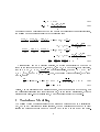
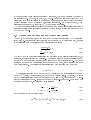
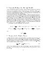
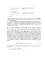
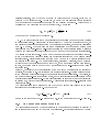
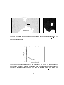
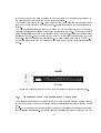
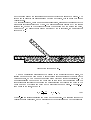
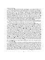
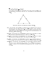
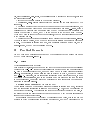
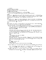
coecient and is the angular velocity of the earth. A schematic representation of some
of these quantities may be seen in Figure 1.
According to the theory of characteristics, if = 0 and the ow is subcritical, two
boundary conditions are to be prescribed at the inow and one at the outow. However,
when considering the case 6= 0, the presence of the diusion term in system (47-48)
requires the imposition of a proper boundary condition for the unit-width discharge on the
whole boundary and, moreover, as is usually very small in the applications, it is natural
to require that these boundary conditions recall the inviscid case as the viscosity coecient
tends to zero. Therefore, the boundary conditions applied here are as follows: as many
Dirichlet conditions as required by the characteristic theory plus Neumann boundary
conditions for each component of the unit-width discharge where its value is not yet
imposed. Note that the weak Neumann condition on q arises naturally in the integration
by parts of the diusive term, when considering the weak form of (47).
13
z
ξ
x
0
-h0
Figure 1: Elevation and depth.
5 The Numerical Scheme for the SWE
The main idea behind the adopted time-advancing scheme is to split the equations at
every time step, in order to decouple the physical contributions. The discretization in
time of the system (47-48) leads to the following equations to be solved:
Step 1
vn = qn=hn ; vn+1=3 = vn X
(49)
Step 2
qn+1=3 = hn vn+1=3
n+2=3 n+1=3
qn+2=3 + t g q h2h1j=q3K 2 j = qn+1=3 + t r rqn+1=3 2
qn+1=3 (50)
Step 3
h
i
n+2=3
qn+1 qn+2=3 + t ghnrn+1 q hn n+1 n = 0
(51)
n+1 n + t r qn+1 = 0
(52)
The symbol vnX indicates the value of the velocity, obtained by a Lagrangian integration
using the method discussed in Section 5.1. At the third step, the equations (51) and (52)
are decoupled by subtracting the divergence of (51) from (52). One then solves the
following Helmholtz{type equation:
n+1 (t)2 r ghnrn+1
n+2=3
+ t r q hn n+1 = n
!
t r qn+2=3 + t r 14
(53)
qn+2=3 n
hn
!
(54)
This new elevation is then used to solve equation (51).
The spatial discretization of equations (50-52) is based on the Galerkin nite element
method; the basic theory of the Galerkin approach may be found, for example, in [1], [3]
and in reference [5], which treats the SWE. The weak formulation of equations (49-52),
is accomplished in a standard way, and is not shown here. An important aspect of the
spatial discretization of equations (50-53) is that two dierent spaces of representation
have been used for the unknowns: the elevation is interpolated by P1 functions, whilst
the unit-width discharge is interpolated by P2 functions. As usual, P1 is the set of
piecewise linear functions on triangles and P2 is the set of piecewise quadratic functions
on triangles. The choice of these interpolation spaces, rst suggested in [4], eliminates
the spurious oscillations that arise in the elevation eld when a P1-P1 representation
is used. To knowledge, no theoretical explanation of incompatibility between spaces of
representation of the unknowns has yet been stated theoretically for the SWE.
main advantage of this fractional step procedure is that the wave traveling at speed
pghThe
is decoupled in the equations and treated implicitly. Therefore, the CFL condition
due to the celerity is cheaply circumvented. Moreover, as the Lagrangian integration is
unconditionally stable and all the terms appearing in eq. (50) are discretized implicitly,
the resulting scheme is unconditionally stable.
A drawback of a fractional step scheme as the one adopted here is that this scheme is
only rst order accurate in time. However, this is not an actual disadvantage as the model
deals with tidal phenomena that vary slowly in time. From a mathematical point of view,
in this fractional step framework one requires, a priori, that the boundary conditions to
be satised by the collection of fractional steps coincide with the boundary conditions to
be satised by the original dierential system, as described in Section 4. Unfortunately, at
Step 3 the solution of the elliptic equation (53) requires the imposition of proper boundary
conditions for the elevation on the whole boundary and, in the practical applications, this
may not be the case. To overcome this diculty, we relax the original requirement and at
this step we impose a Neumann condition on the part of the boundary where the value of
the elevation is not originally given. In the test cases one can observe that this procedure
works well in practice.
In the integration of the weak formulation of eqs. (50) and (51) the lumping technique
has been adopted for the mass matrices of q. By the term \mass lumping" we intend
the use of a low order quadrature formula for the evaluation of the integrals involving the
non dierential terms, yielding a diagonal stiness mass matrix. It is well known that
for P2 elements a nontrivial diagonalization has to be performed (as may be the case
of P1), otherwise a singular matrix is recovered (see appendix 8 of reference [5]). This
diculty has been overcome in the following way: each triangle of the mesh is divided
into four parts by connecting the midpoints of the sides; it is then possible to use the
three vertex-points rule on each subtriangle. The total integral is then the sum of the
subintegrals and automatically leads to a diagonal mass matrix.
A possible objection to this approach is that the mass lumping technique is known
15
to produce large phase errors for unsteady problems, which are precisely the ones we
are interested in. However, at Step 2, no wave-type phenomena are involved and the
dissipation coecient is usually so small that the diusive term can be treated explicitly
without resulting in any additional unphysical constraints. On the other hand, when
considering equation (51), for given n+1 , the equation is explicit.
The computational eort required by this scheme for the solution of algebraic systems
therefore consists of the inversion of one symmetric matrix, with size coinciding with the
number of P1 nodes.
5.1 Lagrangian Scheme for the Convective Terms
At Step 1, the advective part of the momentum equation is integrated by a Lagrangian
scheme [6, 7]. Rewriting the convective terms of equation (47) in Lagrangian form, results
in the solution of two coupled ordinary dierential equations:
dv(X(t); t) = 0
dt
dX = v(X(t); t)
dt
(55)
(56)
The curve X(t) is the characteristic line and its slope is the velocity itself so that, at
this stage, it coincides with the pathline. The velocity eld plays a double role: it is the
unknown to be determined as well as the slope of the characteristic curve. As we are
interested in computing the solution at the nodes of the mesh, let us consider the node
with coordinates y. The initial condition associated with equation (56) must be:
X(tn+1 ) = y
(57)
To integrate equation (56) we need to know the slope of the characteristic curve at y
at time tn+1 which, i unfortunately, is the unknown velocity itself. Therefore, the slope
of the characteristic line has to be approximated in some way, for instance by a zeroorder extrapolation in time. Assuming the use of a second-order Runge-Kutta scheme to
integrate equation (56), the algorithm is as follows:
X = y 2t vn(y)
X(tn ) = y t vn(X )
(58)
(59)
and equations (55) immediately give:
vn+1=3(y) = v X(tn+1 ); tn+1 = v (X(tn); tn)
16
(60)
As the Lagrangian integration requires the primitive form of the equations, the fourth
term that appears in the left hand side of (51) has been added to ensure consistency with
equation (47), which is written in conservative form. We note that, apart from this term,
the discrete counterpart of equations (49-52) requires the inversion of symmetric matrices
only. However, this consistency term is of minor relevance in all the ows in which the
typical time scale is much larger than the time step (as is the case of tides). Therefore,
the usual Conjugate Gradient (CG) algorithm can be condently used in this kind of
simulation.
The Lagrangian discretization of the transport terms has many attractive features: it
avoids spurious oscillations arising due to the centered treatment, without the inclusion
of any unphysical viscosity coecient and it eliminates any restriction on the time step.
However, when using unstructured grids the pathline reconstruction, which requires the
knowledge of the element in which the foot of the pathline falls, consists of a greater
algorithmic eort than that on structured grids. In practice, this diculty has been
overcome in the code by dening an ordered list containing all the elements that are
adjacent to a node or to a given element. In this way the search for the element in which
the pathline foot falls is restricted to clusters of elements. To avoid that the foot of the
pathline reconstructed falls outside of the domain, the rigid boundary of the domain is
always assumed to be a streamline.
It is worthwhile to remark that the quadratic representation of velocities, that has been
adopted for compatibility reasons, fully satises the accuracy requirements recommended
for the reconstruction of the pathline [6].
5.2 Imposition of Boundary Conditions
Particular conditions on the unknowns must be posed on the boundary of the integration
domain. To further investigate which are the dierent possible conditions, we distinguish between open boundaries, across which we can have a net ux of water, and closed
boundaries, i.e. solid walls.
5.2.1 Open Boundaries
In these regions we can impose conditions on the discharge unknown or on the elevation
unknown. We can have Dirichlet b.c. on the discharge, for example at an inow region, to
impose a particular ux of water on that part of the domain, possibly changing in time.
In this case, we will not have conditions on the elevation.
Alternatively we can impose Dirichlet b.c. on the elevation, for example to simulate sea
tides. In this case we usually impose natural b.c. on the discharge, that is the requirement
that the discharge must be normal to the prole of the boundary. This is done projecting
the momentum equation on the normal direction.
17
5.2.2 Close Boundaries
On solid walls we can model the ow in two dierent ways: we can reproduce the physical
situation, in which we nd the water at rest, or we can ignore the friction eect of the
wall, simply imposing a zero ux across the wall. The two dierent models are usually
referred as no-slip and free-slip boundary conditions.
No-slip boundary conditions We impose a null velocity eld all along the closed
boundary, thus
q=0
on the boundary, that is we impose a Dirichlet boundary condition on the unit-width
discharge.
Free-slip boundary conditions We ask for a null ux across the wall, by imposing a null
normal component of the velocity (and thus of the discharge) along the close boundary,
qn = 0
where n is the unit outward normal direction. As we treat the convective terms with a
lagrangian procedure, we must pose this condition in a strong way. It is impossible to
obtain the normal derivative in a weak form. The discretized momentum equations for
the two components of the discharge give rise to two linear systems,
Aqx = bx
(61)
Aqy = by
(62)
(63)
where A is the dierential operator.
Instead of the two systems above, we consider a unique system of the form :
A 0 q=b
(64)
0 A
where q = (qx; qy )T , and b = (bx; by )T . We now couple the equations, solving on the solid
boundary
qxnx + qy ny = 0
(65)
and
A(qxny qy nx) = bxny by nx
(66)
In the code, the rst condition is imposed on the qx variable, and the second on the qy
variable, if jnxj > jny j, and the opposite is done if jny j > jnxj. This procedure ensures
positivity of the diagonal terms of the matrix. Please note that condition (65) imposes a
null normal velocity component, while equation (66) solves the tangential component of
the velocity.
!
18
6 Numerical Scheme for the k " Model
The numerical approximation of the shallow water equations for turbulent ow is almost
the same that was originally developed for laminar ow, and described in Section 5. We
have adopted a fractional step method, where for turbulent ow it has been decided to
adopt only implicit discretization because, by denition, turbulence modeling is used for
ows where diusive eects play a relevant role.
The convection of turbulent quantities is carried out by lagrangian integration, in analogy
to what is done for momentum transport. The source terms are discretized implicitly or
explicitly, depending on their sign. This procedure, known as semi-implicit scheme [1],
reduce the cost of the fully implicit scheme; the idea is to split the terms of order zero
into their positive part and negative part, and treat implicitly the positive terms and
explicitly the other ones. Then all the terms on the left hand side are positive and so are
all the terms on the right hand side. The maximum principle for PDE in the discrete case
insures positive value of k and ". (For physical and mathematical reasons it is essential
that the system of PDE yields positive values for k and ").
The nal scheme for the equations (3) and (4) is then
n
1 + t k"n tr ( + tn )rkn+1 = kn (X ) + tP n + tPkn
(67)
n
n
"n+1 1 + tc2 k"n tr + cc" r"n+1 = "n (X ) + t cc1 k"n P n + tP"n (68)
kn+1
!
!
with
n 2
tn = c (k"n)
7 Transport of a Passive Tracer
A passive tracer is a quantity that is transported by the velocity eld of the uid, but
that does not aect the uid motion itself. It can represent a concentration of a pollutant,
or a thermal eld (where the eects due to the variation of density are neglected). The
equation describing the evolution of the tracer is thus of the form advection-diusion,
with the possible presence of source terms:
@T + u rT 1 r (h rT ) = S
(69)
t
T
@t
h
where T is the vertically integrated value of the tracer, u = (u; v) is the velocity eld of
the uid, h is the water depth, T is the diusion coecient of the tracer and ST is the
source term.
19
This equation is solved in SWEET through the usual algorithms used for the other
equations, that is a lagrangian integration for the advective term and an implicit formulation for the diusive term, giving rise to a linear system, solved through a conjugate
gradient algorithm.
Boundary conditions are imposed only on open boundaries, where the water enters or
leaves the domain. At the inlet, we impose a Dirichlet condition on T , assigning it a given
value (usually zero). At the outlet, we impose the value resulting from the integration of
the advective term.
8 Parallelization Strategy
In the numerical scheme described above, two \computational kernels" can be recognized.
For equations (50-52), since all terms but qn+2=3 are evaluated at previous time levels,
the nite element formulation of equation (50) gives
M qn+2=3 = g
(70)
where g is a known vector and M is the nite element mass matrix, i.e.
Mij =
Z
d
i j
(71)
fig being the set of nodal shape functions which provide a basis of piecewise linear
polynomials. By adopting a mass lumping technique [3], the solution of the Step 2 is
explicit and therefore the main computational eort reduces to the following tasks:
1. Lagrangian integration of the convective term as dened by equations (55-56).
2. Solution of the elliptic problem dened by equation (53).
8.1 Mesh Partitioning
The strategy devised for the parallelization of the above listed computational kernels is
based on domain decomposition. This technique exploits the topology of the problem,
partitioning the computational domain into subregions. The fact that we are dealing
with unstructured meshes poses some additional problems for the implementation of the
parallel algorithms, both for dening properly the decomposition into sub-domains and
for the denition of an ecient communication scheme. However, the exibility ensured
by unstructured grids is a remarkable advantage of the nite element technique when
dealing with complex geometries (as it is often the case in environmental ows) and it
makes the eort worthwhile.
The rst step for a domain decomposition approach is the partition of the computational domain into a given number of sub-domains. The specications characterizing such
partitioning should be:
20
1. Minimization of the number of neighbors for each sub-domain.
2. Minimization of the number of nodal values at interfaces between sub-domains.
3. Balancing the size (i.e. the number of nodes) of each sub-domain; this will result in
a balancing of the computational load between the dierent processors.
To perform the partitioning we have tested three software packages, Metis [11], Chaco [9]
and TopDomDec [10], which implement several algorithms. The interested reader may
consult the given bibliography for details. Our parallel procedure requires that the subdomains partially overlap each other. This feature has been obtained by developing an
ad-hoc software.
8.2 Lagrangian Integration of the Convective Term
The Lagrangian integration of the convective term requires the calculation of the pathlines
and the evaluation of the velocity where the pathline falls. On an unstructured grid
the major computational cost consists in recognizing which elements are crossed by the
pathline. In practice, this operation requires, for each node and at each integration step,
the computation of the area of some triangles for each mesh node. This formulation for
the Lagrangian integration of the convective term does not require any matrix inversion.
It is then a local operation, which needs for each node some information about the old
solution in a cluster of elements around it.
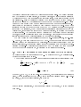
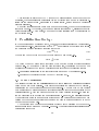
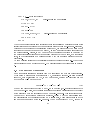
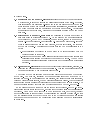
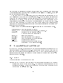
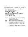
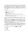
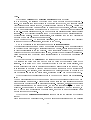
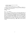
The Lagrangian integration of the convective terms can naturally be performed in
parallel in a domain decomposition framework. Each processor carries out the integration in the nodes belonging to the sub-domain assigned to the processor itself. As the
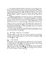
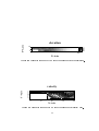
pathline can exit the sub-domain, care must be used when dealing with the nodes posed
in proximity of its boundary. The Lagrangian integration of the nodes belonging to the
overlap region must be computed by the processor which succeeds in the reconstruction
of the pathline. With regard to the nodes in the proximity of the overlap, a limit on the
time step is dictated by the requirement that their pathline does not exit the sub-domain
to which they belong. This means in practice that the CFL velocity number should be
smaller than 2:
jvj )t 2
max
( x
(72)
Such a condition is not restrictive in practical applications, where the wave celerity is
usually much larger than the uid speed.
8.3 Parallel Solution of the Linear System
Equation (53) can be seen as a particular case of elliptic dierential problem of the form:
21
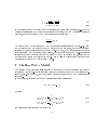
yn+1
Ω2
yn+1
Ω1
δΩ1
yn
δΩ2
pathline
overlap
Figure 2: Lagrangian integration at the boundary between sub-domains.
Lu = f;
(73)
where u = n+1 , L = L(n ; H; qn+2=3; t) indicates a quasi-symmetric linear operator
and
f = f (n ; H; qn+2=3; t).
After being approximated by nite elements, relation (73) can be written in the algebraic
form:
Ax = b
(74)
The matrix A is symmetric, positive denite, sparse and, typically, very large. An eective
algorithm to solve the linear problem (74) is the conjugate gradient (CG), when coupled
with a suitable preconditioner.
We use a parallel implementation of a CG to solve equation (74) on a distributed
memory machine. An eective parallelization of this iterative method can be be obtained
as follows. Let us suppose that the computational domain is partitioned into N subdomains i, with an overlap of one element, such that = i i. We assign at every
processor the job of performing the computations on the elements of the matrix belonging
to a sub-domain i. The following pseudo-code focuses the communications needed in
the parallel version of the algorithm, see for instance [15].
S
r0 := b Ax0; p0 = r0
For j = 1; ::::: until convergence
22
j = (rj ; rj )=(Apj ; pj )
xj+1 = xj + j pj
rj+1 = rj j Apj
j = (rj+1; rj+1 )=(rj ; rj )
pj+1 = rj+1 + j pj
end do
inter-processor communication!
inter-processor communication!
A look at the algorithm listed above shows that the iterative method can be parallelized
by exchanging information only when global scalar quantities are computed; this occurs
twice in each iteration.
An ecient implementation of a standard preconditioner is not straightforward. In
fact, neglecting the trivial case of diagonal preconditioning, eective techniques such as
incomplete LU decomposition are intrinsically sequential. We can indeed say that the
main eort in nding an ecient parallel iterative solver has to be spent in devising the
appropriate preconditioner.
8.4 Additive Schwarz Preconditioning for the Elliptic Problem
In what follows, we briey outline the additive Schwarz preconditioner, more details on
the theory being available, as example, in Ref. [12]. The method of Schwarz has been
originally proposed as a solver. The underlying idea is to solve the elliptic problem
separately on some portions of the original integration domain, exchange information at
the borders of the dierent portions, and then iterate the procedure till convergence,
obtaining, from the union of the solutions on sub-domains, the global, exact solution of
the original problem. In recent years this view of the Schwarz method as a solver has
been practically abandoned, whereas its attractive features as a preconditioner have been
exploited. We dene Ri as the restriction operator relative to the sub-domain i and
Ai = RiARTi . Note that, from a functional point of view, Ai is the local stiness matrix
in i as arises when imposing homogeneous Dirichlet boundary conditions on @ i. If we
consider
M 1=
X
i
RTi Ai 1Ri where Ai = Ri ARTi
(75)
the parallel conjugate gradient algorithm preconditioned with the Additive Schwarz method
then reads:
r0 := b Ax0; z0 = M 1r0; p0 = z0
23
For j = 1; ::::: until convergence
j = (rj ; zj )=(Apj ; pj )
inter-process communication!
xj+1 = xj + j pj
rj+1 = rj j Apj
zj+1 = M 1 rj+1
j = (rj+1; zj+1)=(rj ; zj )
inter-process communication!
pj+1 = zj+1 + j pj
end do
The Schwarz preconditioner is an attractive choice for parallel computations because of its
locality: it does not require any exchange of information between sub-domains. Moreover,
because of the denition of the restriction operator Ri, the elements of the matrix M are
identical to the ones that are in the matrix A, so that no specic storage is required for
the preconditioner. Finally, it may be noted that the local subproblems to be solved at
the preconditioning level are always well posed because they can be seen, at a functional
level, as the discretization of a Poisson problem with homogeneous Dirichlet boundary
conditions.
An open question refers to of the possibility of solving the local problems (i.e. the Schwarz
preconditioning) in an approximate way. We will discuss further this subject in Section
9.
8.5 Coarse Grid Correction
Some theoretical results are available from the analysis of the Schwarz preconditioner.
When using a regular grid of spatial step x, partitioned into sub-domains of linear
length H , with overlap size = H , it may be shown [8, 12] that the condition number
of the matrix M 1A is bounded as
cond(M 1A) CL 2(1 + 2)
(76)
where C is a value independent from H and . In 2D problems, H 2 is proportional to the
number of sub-domains, and therefore this estimate reveals a deterioration of the quality
of the algorithm with the increase of the number of sub-domains. This inconvenience can
be removed by introducing a coarse grid operator. Let's AH be the matrix arising from
the discretization of the elliptic problem on a coarse grid, whose element size is of the
same order of magnitude of the sub-domains. Then we can replace M by Mc, dened as
24
Mc 1 = RTH AH1RH + M 1
(77)
Here, RTH is the prolongation map from coarse to ne grid, given, for example, by a
piecewise linear interpolant from coarse grid nodes. It can be shown that
cond(Mc 1 A) C (1 + 1)
(78)
where, again, C is independent from H and . Thus, the preconditioning property of the
operator Mc does not depend on the number of sub-domains, but only on the amount of
the overlap between them.
The coarsening of an unstructured grid can be a non-trivial task. Therefore, we have
investigated a dierent procedure for the construction of the coarse grid operator AH ,
by resorting to an agglomeration technique similar to that introduced in [13, 14] in the
context of multigrid procedures. We consider RH so that
AH = RH ARTH
(79)
where
8
<
RHij = 1 if j 2 i [ @ 0 otherwise
The construction of AH is thus a completely algebraic procedure and it does not require
to build a coarse triangulation. There are no theoretical results concerning this operator.
We have therefore resorted to numerical investigations to test its eectiveness; in Section
11.3 some computational results are shown and the performance of this algebraic coarse
grid operator is discussed.
After these details, it clear that the choice of this Schwarz preconditioner has been guided
by its intrinsic parallelism and its ability to ensure, when the coarse grid correction is
used, a behavior independent on the number of sub-domains, and thus on the number of
processors, used in the calculation.
:
8.6 Parallelization of the k
"
model
As explained in Section 6, the equations for the k and " quantities are solved using the same
numerical methods for the integration of the advective and diusive terms of the equation
for the momentum, that is a lagrangian integration for the advective terms and a conjugate
gradient to solve the linear system arising from a semi-implicit formulation of the diusive
term. Thus, no new algorithm are introduced in the code, and the parallelization of the
k " model follows the same strategy stated above.
25
8.7 Parallelization of the Transport of the Scalar Tracer
Exactly the same considerations given above hold for the advection-diusion equation for
the passive tracer.
9 Parallelization: Implementation Details
Even if the sub-domains overlap each other there is only one sub-domain where a given
node i is considered as interior. This sub-domain will be termed as the parent sub-domain
for that node.
The domain decomposition approach can be easily applied to the explicit parts of algorithms, since the operations are mainly local. The nodes at the boundary between subdomains must be updated at the end of each step, by receiving the values from their parent
sub-domains. Thus, lists of sending and receiving nodes are dened for every sub-domain,
together with a communication pattern able to guarantee no-blocking communications.
During the Lagrangian step (Step 1), the situation is complicated by the fact that
for a border node it is possible that the pathline falls outside the sub-domain. Thanks
to the overlap, it is possible to perform the Lagrangian integration in the neighboring
sub-domain. However, the list of the border nodes for which the pathline falls outside the
sub-domain can change at each temporal iteration, depending on the velocity direction. A
dynamic mechanism has then been devised for the denition of the sending and receiving
nodes.
The integration of the implicit equation for the elevation at Step 3 poses dierent
problems from the point of view of the parallel implementation of the algorithm. The CG
is parallelized in a genuine domain decomposition way: the matrix, the right hand side and
the unknown vector are distributed among the processors, and the matrix-times-vector
and vector-times-vector operations are performed in parallel on the distributed set of data.
Again, the communication scheme has been designed to avoid blocking patterns. The
interprocessor communications doesn't make any use of pre-dened collective messagepassing instructions, but only the base instructions send and recv of the PVM [17]
message passing library. In this way the code portability is assured and its performance
is reproducible.
As discussed in the previous Section, the CG is preconditioned by an additive Schwarz
algorithm. To exploit all its capabilities, we decided to have the number of sub-domains
for the Schwarz algorithm be independent from the number of processors. We have thus
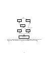
introduced a second level of subdivision into domains, so that several sub-domains can be
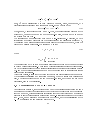
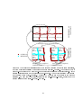
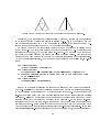
assigned to a single processor. We rst partition the domain into a number of portions Np
equal to the number of processors, then each portion is further subdivided into the nal
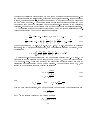
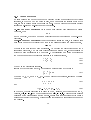
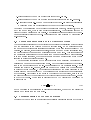
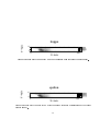
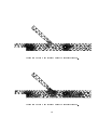
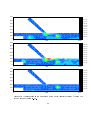
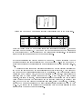
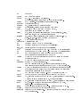
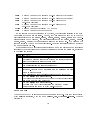
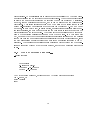
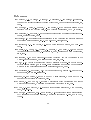
sub-domain pattern. A schematic representation of this two levels partition is presented
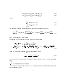
in Figure 3.
26
PROCESSOR
3
PROCESSOR
4
PROCESSOR PROCESSOR
5
6
PROCESSOR
7
PROCESSOR
8
FIRST LEVEL
OF SUBDOMAINS
PROCESSOR PROCESSOR
1
2
Inter-processors communications
OVERLAP
REGIONS
LOCAL
CG+
ILUT
LOCAL
CG+
ILUT
Intra-processors (implicit)
communications
LOCAL
CG+
ILUT
LOCAL
CG+
ILUT
LOCAL
CG+
ILUT
LOCAL
CG+
ILUT
SECOND LEVEL
OF SUBDOMAINS
LOCAL LOCAL
CG+
CG+
ILUT
ILUT
Intra-processors (implicit)
communications
Figure 3: The two level of partitions used in the code: we imagine a run over eight processors,
and thus a rst level partition of the global domain in eight sub-domains. The detail on the two
rst sub-domains shows how every sub-domain is further partitioned in several regions. All the
explicit integrations act on the rst level of sub-domains. The Schwarz algorithm acts locally
on the second level of sub-domains. The global CG uses the same data sets of the Schwarz
algorithm. In dark grey the overlap regions for the rst-level sub-domains, in light grey the
overlap regions for the second-level sub-domains.
27
Using a large number of sub-domains for the Schwarz algorithm may produce a considerable reduction of computational time. In fact, the solution of many small linear
systems can be faster than the solution of few linear systems of larger dimension. The
distribution of the matrix and vectors for the global CG is made at the second level of subdomains: in this way the same data structures are used for carrying out both the global
CG and the Schwarz preconditioning, thus optimizing the memory requirements. This
choice greatly complicates the managing of the communications for the global CG. To gain
the maximum eciency, we have set up a scheme that uses implicit communications via
common blocks when the two communicating sub-domains reside on the same processor,
and explicit message-passing instructions when the communication involves two dierent
processors. Moreover, to minimize the latency time, all the messages from sub-domains
residing on one processor, that are to be delivered to sub-domains all residing on another
processor, are rst collected in a buer and then sent with a unique send instruction.
The linear systems local to the sub-domains resulting from the Schwarz algorithm are
governed by the matrix Ai, which is positive denite. Therefore, we have decided to use
again a CG procedure, preconditioned with an incomplete LU decomposition (ILUT)[15],
for their solution. On the contrary, the coarse grid system is always solved \exactly", by
inverting the matrix AH . We will refer to the CG iterations at sub-domain level used to
solve the Schwarz preconditioning system as the \local" CG.
Since the local CG has to work just as a preconditioner, the solution of the subsystems
would preferably be carried out with a low degree of accuracy. This would correspond
to use an approximation of the preconditioning system. In practice, however, we have
noted that the convergence rate of the global CG is heavily dependent on the accuracy
of the local solutions. We thus have coupled the convergence thresholds of the local and
the global CG's so that the values of the local residuals are always lower than the current
value of the global CG residual. In this way we have obtained a good overall convergence
rate.
The pseudo-code of the parallel shallow water model thus reads as follows:
do i = 1, number of time steps
solve Lagrangian transport in each of the Np sub-domains
exchange boundary conditions among the Np sub-domains
solve Step 2 in each of the Np sub-domains
exchange boundary conditions among the Np sub-domains
do until convergence
precondition solving local linear systems on each of the Ns sub-domains
by CG + ILUT
perform one CG iteration on the global domain (in parallel)
28
end do
solve Step 3 for the unknown q in each of the Np sub-domains
exchange boundary conditions among the Np sub-domains
end do
10 Mesh Adaption
The use of unstructured grids for the numerical approximation of partial dierential equations of applied mathematics has two great attractives. The one most commonly claimed
is the geometrical exibility, that is the capability to handle computational domains with
complicated boundaries of problems that would be almost impossible to solve by a structured approach. However, there is a second aspect of unstructured grids that has even
more relevance: the possibility to rene the computational mesh where needed, in order
to minimize the computational error in some proper sense. Suitable indicators of the
accuracy of the solution allow to rene the mesh where the numerical error is large and
to coarsen it where the error is small, in order to optimize the quality of the computed
solution for a given computational eort. [22]
Mesh adaption techniques have been used since many years ago in several elds of
computational uid dynamics, but adaptivity has not yet much explored in the framework
of free surface hydrostatic ow. At out knowledge only a very recent paper [23] compares
and discusses the use of high order polynomial basis (p adaption) for discretization of
the shallow water equations versus local mesh renement, where the the order of the
polynomial approximation is kept unchanged (h adaption).
The mesh adaption technique adopted, (see section 10.2) is based on the use of a
background grid (see for example [24], [25]). The numerical simulation starts on a grid,
possibly composed by few nodes, which is the coarsest mesh used in the computation: its
nodes are neither moved nor suppressed. Successive levels of renement and coarsening lie
on the background grid. This technique has been adopted because of the very complicated
geometry of the boundary that characterizes environmental applications in river, coastal
areas and so on. By keeping a background grid, the information about the position of
the boundaries and bathymetry can be preserved and is not lost by further interpolations
due to node movements. Remarkably, a relevant by-product of the mesh adaption is that
poor care has to be used in dening the initial grid: "with adaption, any initial grid will
be transformed into a near optimal discretization". [26]
A peculiar aspect of the mesh adaption for shallow water ow is the necessity to
devise proper indicators of the numerical error that should drive the grid renement and
de-renement. In the present paper three possibilities are proposed and investigated: the
second order derivative of the elevation eld, the second order derivative of the magnitude
of the velocity and the local mass conservation in a specic sense. Every error indicator has
29
a mathematical basis or is suggested by numerical or physical reasons. The performance
of these error estimators is discussed together with the numerical results in the last section
of the paper.
10.1 Error estimate and error indicators
The mesh adaption technique requires some a posteriori estimate of the error of the
numerical solution based on the computed solution itself: it is necessary to state locally
how much the numerical solution diers, in a proper sense, from the exact solution of
the dierential problem. In this section we propose a few ways to determine where the
computational mesh should be rened or coarsened.
1. For linear elliptic problems it is possible to estimate rigorously the numerical error
in terms of the second derivative of the exact solution. Let u be the exact solution of the
elliptic problem : ru = v; that is, in weak form
(ru; rv) = (b; v)
(80)
for all v belonging to a suitable space and where ( ; ) indicates the usual internal product
in L2. Then, given a triangulation with maximum side length h, it can be shown [27] that
the distance between the exact and the computed solution linear uh in H 1 is bounded as
follows:
u j
j
(r(u uh); r(u uh)) = k r(u uh) k2L2 h2 max
ij x x
i j
(81)
As the computational kernel of the numerical scheme adopted in section 4 is an elliptic
equation for the elevation of the water , in the rening{coarsening stage we can use
the estimate (81), where the right hand side has to be calculated using the computed
solution uh. The error estimate (81) suggests to dene the following non{dimensional
error indicator:
1;m = h m max
j
m ij
X
k
k
Z
k m d
j
xi xj
(82)
where is the computational domain and k is the k-th linear basis function.
2. From a more physical point of view, considering the whole shallow water equations
system, it can be foreseen that there are typical behaviors of the oweld that the error
indicator 1 could not be able to detect properly. For instance, shear layers between
30
parallel velocities, as may happen at inow of branches into a channel, could not be
detected by the indicator (82). To this aim, it would be more useful to use an indicator
of the gradients of the solution depending on the velocity magnitude. Extending in a
heuristic way the denition (82) to the velocity eld, we propose
2;m = max
j
ij
X
k
where v is the magnitude of the velocity v.
vk xk xm d
j
i j
Z
(83)
3. An important feature that a numerical scheme for shallow water ow should possess
is mass conservation. This property is accomplished by the scheme described above, as
the discrete equations are obtained from the continuity equations, and are then consistent
with it. However. the nite element scheme illustrated above does not ensure mass
conservation in a nite{volume cell{centered sense: the mass variation inside a triangle
during a time step is not exactly equal to the ux through the edges of the triangle itself.
The reason of this is twofold. On one hand the use of quadratic polynomials to approximate the discharge q yields to larger computational stencil than when using a linear
representation. Mass conservation checking must be done an a stencil consistent with
the stencil of the scheme. The mass conservation, triangle by triangle, can be properly
advocated only for nite elements of mixed type, when a special mass lumping is used.
In fact, nite elements of mixed type RT0 just recover the cell{centered nite volume
technique [28].
Secondly, we observe that the substitution of the momentum equation into the continuity
equation, that leads to eq.(53) involves a new spatial derivation. This is a usual approach
in the nite elements context [29], but does ensure local mass conservation. Conversely, in
the nite dierence-nite volumes framework, such a substitution is usually carried out at
an algebraic level: equations (51-52) are rst discretized in space and then the substitution
is carried out, without further derivatives. This ensures local triangle-by-triangle mass
conservation [30].
The considerations above suggest to use the check of local mass balance as an error
indicator for the present scheme. We dene then
3;e = j 1t e(n n 1 )d
+ e q d j
Z
I
(84)
Here is the contour of the e-th element and 3;e is the mass defect in the e-th element.
10.2 The mesh renement technique
Any error estimator among the ones described in the section above allows to identify a
set of elements of the mesh to be rened (or coarsened). Several techniques can be used
31
to this aim [26].
1. Repositioning of the mesh (r-methods): local renement of the mesh is obtained
moving nodes, in order to minimize the distribution function of the error. Of course,
this local renement generates de-renement in the remaining part of the domain.
Since topology of the mesh does not change during repositioning, this strategy is easy
and cheap to implement: the connectivity of the grid is unchanged. Nevertheless
it is a strategy not often used, because of the constrain of using a xed number of
elements.
2. Enrichment of the mesh (h-methods): the triangles of the grid are divided in
elements of lower average side length h. As the error of the numerical solution
behaves like ch, with c and constants, these methods, if used in a proper way,
ensure -power convergence. For this reason h-methods are most popular. although
their implementation is more complex because, at every subdivision, the topology
of the mesh changes. The splitting of the elements can be made essentially in two
ways:
1. edge bisection: midpoint of an edge marked to be rened is joined with the
vertex opposite to this edge.
2. standard renement: a marked triangle (father) is subdivided into four similar
triangles (sons) joining midpoints of the edges of the father. The number of
edges and triangles increases for a factor four and the local length of triangles
is halved.
3. Re-meshing (m-methods): to produce a highest quality triangulation, creation, destruction and repositioning of the nodes is allowed. This is a more general procedure
but also heavier from a computational point of view.
The choice of the more suitable mesh adaption procedure depends on the problem
at the hand. For example, regularity of the element size length and shape can be a
requirement or not. In compressible ow simulations, very stretched elements are useful,
because where shocks are located, the ow direction is strongly biased. Adapted grids for
these problems are in general very irregular both in side length and in shape ([22]). The
more appropriate strategy for these kind of problems seems to be the h-method 2.1.
In the present paper we chosed to use the renement technique 2.2 of the h-method.
Main reason for this choice is that the h-methods keep the information on the original grid
unchanged. When a new node is added in the middle of an edge, bathymetry, velocity
and water elevation in it are obtained by interpolating the values in the element. In this
way the original values of the bathymetry and of the physical unknowns in the initial
mesh are never abandoned and the degradation of the solution due to the interpolation
is minimized.
32
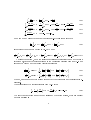
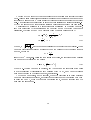
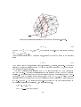
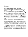
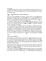
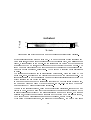
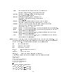
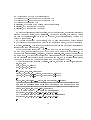
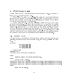
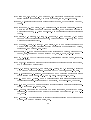
Figure 4: Red Renement (standard or regular) and green of a triangle.
Moreover, when simulating subcritical shallow water ow, regions are more suitable
to be rened instead of lines (see results in section 11.5). So, in the present work the
computations are started on a mesh as regular as possible, then renements and derenements are accomplished in such a way to preserve regularity.
In Figure 4 is shown the subdivision technique known as standard or regular or red
renement [31]. The marked elements are rst divided in standard way. The surrounding
triangles have then one, two or three edges sub-divided. The nodes in the midpoint of
the edges of the elements not yet rened are called \hanging nodes". Elements having
hanging nodes must be rened in a proper way to ensure consistency of the triangulation.
Among the possible strategies, we have chose the one described in the following, in C-like
form:
for (i=0;i<NEL;i++)
if(Err(i)>thresh) StandRef(i);
for (i=0;i<NEL;i++)
if((NHang(i)>1) || (NHang(i)==1 EType(i)==green)) StandRef(i);
if StandRef has been called at least one time in the last block then
it is re-executed;
for (i=0;i<NEL;i++)
if(NHang(i)==1) MakeGreen(i);
is a function evaluating the error on the triangle i with one of the described
methods.
renes the triangle i in standard way; if the triangle is \green",
it and the sibling are substituted by the father before renement. When executing rst
for-block only elements which have an error greater than a xed error threshold thresh
are rened. NHang(i) and EType(i) are functions which respectively return number of
hanging nodes and type (standard or green) of the triangle i. In the second for-block
triangles which have more then one, or green ones which have at least one hanging node
are standard rened. If some element has been rened maybe some other hanging node
has been created and for this reason this last block is re-executed till possible. In the last
block MakeGreen green-renes triangles which have an hanging node, to ensure consistency
Err(i)
StandRef(i)
33
of the mesh.
This algorithm converges in a nite number of iterations; at most all the elements of the
initial grid will be standard rened. The grid rened with the algorithm listed above has
a minimum number of green elements, which are the elements deteriorating the quality
of the initial mesh.
10.2.1 Pre-renement and mesh enhancement
If some of the characteristics of the solution of a given problem is known a{priori it is
possible, in principle, to decide some sort of pre{renement of the mesh. For this reason
a package named prerene has been prepared which read the initial mesh (in SWEET
format) and a vector of integers containing ags to the elements to be rened and re{write
a le (in the same format) with the new mesh pre{rened.
As already mentioned, the renement technique here adopted, generates at the boundaries of a rened area elements of poor quality. When pre{rening the initial mesh such
drawback can be avoided improving the overall mesh quality by means of an algorithm
known as \Laplacian smoothing".
Given a generic node P of the mesh not in the boundary, we will call patch around P
the polygon formed by all the elements which have this point in common. The information
about elements which constitute the patch is contained in the structure VVER (see section
14. Smoothing of Laplace consists in moving every internal point of the triangulation to
the baricentrum of the patch around this point. This can be done without problems when
the patch is convex. When instead the patch is concave the algorithm must be modied
in order to avoid that the node movement would produce an inconsistent triangulation.
The modied Laplace Smoothing used in the pre{rene module is described in detail in
[32].
Rening and coarsening
When designing a practical strategy of mesh renement-coarsening, it would be very
useful to state rst an acceptable numerical error and then use it as a yardstick: coarsen
the mesh where the error indicator is lower than the reference one, rene when larger.
Unfortunately, the error indicators described above only give, at best, estimates of the
numerical error, or hints about where the error is larger: they do not ensure any absolute
evaluation of its magnitude.
When computing steady ows, this diculty is overcome stating rst the computational
resource that can be addressed, that is the maximum number of nodes to be used in the
numerical simulation. Then, starting with a quite coarse mesh, it is rened until that the
desired number of nodes is reached.
When dealing with unsteady ow, also coarsening is useful. In this paper we are addressing
smooth ow, that is subcritical shallow water ow or, at most, locally transcritical ow.
In such regime there are no discontinuities in the physical variables and, typically, the
34
time-dependency is due to the change of boundary conditions which is smooth in time
and has a period of 12-24 hours. As time goes by, the oweld changes and a proper mesh
adaption strategy should modify the mesh, rening it in a optimal way with respect to
the adopted error indicator. In this framework, instead of keeping constant the number
of nodes, as was the case of steady ow, it is more signicative to keep constant the
maximum error indicator of the grid at any time. This ensure a constant control of the
error all along the simulation.
11 Test Cases
To validate the numerical scheme and its sequential and parallel implementation, we
consider dierent examples. The rst two test problems have been specically designed
to test the discretization of the nonlinear terms in the equations and the mass-conservation
property of the numerical scheme. In addition, they are used to test for the presence of
spurious oscillations arising due to the boundary conditions. The third example is a
demonstration of the parallel performance of the code.
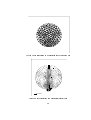
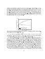
11.1 Jet in a Circular Reservoir
The rst problem is the simulation of a steady jet in a circular reservoir; the details of this
classical test case as well as the experimental results can be found in [19]. The geometry
of the boundary and the computational grid are shown in Figure 5. We use an eddy
coecient = 2:5 10 4 m2=s and a time step of 2 s. The computed velocity eld is shown
in Figure 6. The solution does not dier much from the one shown in [6] and [19]; the
location of the gyre centers are suciently well described, but the maximum computed
velocities in the gyres are underestimated, mainly in the region near the inow. Such a
discrepancy is due to three-dimensional eects, and not to the staircase boundary that
characterizes the nite dierence contours used in the cited references.
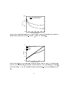
11.2 Hydraulic Jump
The second test case that we consider is the steady 1D ow in a prismatic channel, without
diusion and bottom friction eects. Under these hypotheses the SWE reduce to
q = (Q; 0)
h = h(x)
d
dh = gh dh0
+
gh
dx h
dx
dx
where Q is the (constant) unit-width discharge. If the bottom eld is dened as:
!
Q2
35
(85)
(86)
Figure 5: Jet circulation in a reservoir: computational mesh
0.05 m/s
Figure 6: Jet circulation in a reservoir: velocity eld
36
2
h0(x) = H + x Q2g H12
1
;
(87)
(H + x)2
where H and are constant values, it can be easily veried that the equation (86) has
the following exact solution:
h(x) = H + x;
!
q(x) = Q:
(88)
This test case allows for the verication of the accuracy of the scheme when a strong
gradient is present in the bathymetry, as often occurs in rivers.
The computation for this test has been carried out using an inow depth H = 4, an
inow unit-width discharge Q = 4 and a bottom slope = 0:06. Although this test is
essentially one-dimensional, an analogous case for the 2D code has been run on a channel
300 m. long and 4 m. wide. The computational mesh is almost regular, it is composed
by 580 elements and a detail of it may be seen in Figure 7.
9.786
0
−4.949
110.2
120
130
140
Figure 7: A detail of a regular mesh used in test case 2.
For the boundary conditions, the value of Q has been imposed at the inow whilst
the value of has been imposed at the outow. Figure 8 contains two graphs: a plot of
the exact elevation versus the computed elevation and a plot of the computed unit-width
discharge. The former plot evidences the good accuracy of the scheme for the elevation
as well as the fulllment of the mass conservation property with a small loss of 0.5% for
this mesh.
It should be mentioned that a very large number of time steps were required to reach
the steady state solution, since no mechanism to dissipate the spurious components of the
initial conditions is present in this computation.
37
4.040
0.040
0.030
discharge (m*2/s)
4.020
elevation (m)
0.020
0.010
-0.010
50.0
3.980
exact
computed
0.000
100.0
150.0
x (m)
200.0
4.000
250.0
3.960
0.0
100.0
200.0
300.0
x (m)
Figure 8: Water elevation and unit-width discharge for the 1D test case.
11.3 Parallel Computation on a Complex Geometry
The parallel code has been used for the simulation of the marine circulation in the Bocche
di Bonifacio, the strait separating the Corsica and Sardinia islands in the Mediterranean
sea. In this model, it is assumed that no stratication occurs and that the water circulation
is essentially driven by the tidal boundary conditions, the wind stress and the Coriolis
force. This hydrodynamic problem is characterized by a substantial complexity of the
geometrical data.
We have used a mesh composed of 75053 elements and 38303 vertices. The total
unknowns of the problem are 38303 elevation nodal values and 151661 discharge nodal
values (for every component). The size of this problem does not t into the memory of a
single processor (with 128 MB of RAM), and a minimum of two processors of an IBM-SP2
must be used.
We rst analyze the numerical behavior of the Schwarz algorithm with respect to the
number of sub-domains. In Figure 10 is shown the CPU time required by one global
CG iteration versus the number of sub-domains Ns, for a xed number of processors.
The Schwarz algorithm runs faster when a large number of sub-domains is used, until
the communication overhead for the global CG becomes relevant, eventually preventing
further time savings.
To evaluate the overall code performance, this result has to be considered together
with the result shown in in Figure 11, where we illustrate how the number of global CG
iterations varies with the number of sub-domains. The preconditioning capability of the
38
CORSICA
SARDINIA
Figure 9: On the left: the computational domain for the Bocche di Bonifacio test case. On the
right: a detail of the computational mesh for the zone indicated in the left gure. The entire
mesh has 75053 elements.
4.0
Time (sec)
3.0
2.0
1.0
0.0
2
40
80
120
160
Number of subdomains
200
240
Figure 10: Schwarz preconditioning: CPU time required by one global CG iteration versus the
number of sub-domains Ns , using two processors. Here, the coarse grid correction is used; the
case without correction present the same curve, since the inversion of the coarse system does
not take a signicant amount of time (around 2% for the case with 240 sub-domains).
39
original Schwarz algorithm degrades when the number of sub-domains increases. However,
the algebraic coarse grid correction halts this degeneration completely when more than
ten sub-domains are used. By joining the results shown in Figures 10 and 11 we obtain
the curve for the total CPU time needed to solve the linear system, versus the number
of sub-domains, for a xed number of processors (Figure 12). The best performance for
the present test case has been obtained with 200 sub-domains. This result demonstrates
the usefulness of choosing the number of sub-domains independently from the number of
processors actually used in the calculation.
Number of global CG iterations
300
200
100
No coarse grid correction
Coarse grid correction
0
2
40
80
120
160
Number of subdomains
200
240
Figure 11: Schwarz preconditioning: number of global CG iterations required to reach convergence versus the number of sub-domains Ns .
We now examine the parallel performance of the code, by varying the number of
processors and keeping xed the number of sub-domains for the Schwarz preconditioner;
in the present case, we have used the partition of 200 sub-domains.
In Figure 13 the total speed-up of the shallow water code is shown. As it can be noticed,
both the Lagrangian integration and the Step 2 integration (which are explicit) show a
speed-up which is very near to the ideal one. The speed-up of the implicit step, while not
being ideal, is however satisfying. Since this step has the major computational cost, its
behavior reects largely on the total speed-up (continuous line). The odd behavior of the
curve (the rst derivative does not decrease monotonically, as it would be expected), is
due to the particular setup of sub-domains we use: the shape of the sub-domains for the
preconditioning step changes every time the number of processors changes, even if their
number and size do not. Thus, since the speed and the preconditioning properties of the
Schwarz algorithm can be inuenced also by the shape of the sub-domains, we can need
dierent numbers of iterations for the global CG to reach the given convergence threshold.
In order to further test the behavior of the Schwarz algorithm, we have run the same
40
300.0
No coarse grid correction
Coarse grid correction
Time (sec)
200.0
100.0
0.0
2
40
80
120
160
Number of subdomains
200
240
Figure 12: Schwarz preconditioning: CPU time required to achieve convergence of the conjugate
gradient solver versus number of sub-domains Ns , using two processors.
8.0
Lagrangian Integration
Step 2
Step 3
Total
Speed up
6.0
4.0
2.0
0.0
2
4
8
12
Number of processors
16
Figure 13: Speed-up of the whole shallow water code, for the mesh composed by 75053 elements.
Due to memory requirements, this problem runs on a minimum of two processors, so the speedup are normalized by the two processors value; the ideal speed-up for 16 processors is thus
8.
41
problem on a coarser mesh, to have the possibility of also performing the simulation on a
single processor. The sequential code has been run using an ecient preconditioner, that
is an Incomplete LU decomposition (ILUT). The reduced mesh is composed by 39170
elements and 20169 vertices. We have done both serial and parallel runs, using a RISC
processor of the system IBM-SP2, with 128 MB of RAM. In Figure 14 we report the timing
8.0
Sequential: ILUT prec.
Schwarz + coarse grid prec.
Time (sec)
6.0
4.0
2.0
2
4
6
Number of processors
8
Figure 14: Implicit step: time for the solution of the linear system, on a mesh of 39170 elements.
The horizontal line refers to a sequential run, using an ILUT preconditioner. The other curve
refers to parallel runs, on 2, 4, 6 and 8 processors, with the Schwarz preconditioner.
for the solution of the linear system at the implicit step. The horizontal line represents
the time needed by the scalar run, for the case with ILUT preconditioning. We can see
that the Schwarz preconditioning gives better performance with respect to the sequential
ILUT algorithm when more than three processors are used.
11.4 Abrupt enlargement of a channel; the k
model
To validate the k " model described above, it has been chosen the test case discussed
in [35], corresponding to the ow in an abrupt enlargement of a prismatic channel. The
geometry of the problem may be seen in g.1; it has been supposed that the channel is
4 meters deep and the incoming ow has unit width discharge of 3 square meters per
second. The ow is expected to separate at the edge of the enlargement, with consequent
recirculation.
The most interesting aspect to be compared with experiments is the length of the recirculation zone: the reattachment length for a geometry as the one showed in in g.15
should be slightly less than six times the width of the enlargement, if the ratio of the
width of the former part of the channel over the depth is nearly one [36]. It is worthwhile
42
to remark that such an estimate assumes no dependence of the reattachment length on
the roughness of the channel and on the inowing velocity.
The velocity eld plotted in g.17 shows that the computed solution has a reattachment
length which is smaller then the expected one. This is accordance with the results showed
in [35].
The use of wall functions, at least when using a mesh not stretched at the boundary,
yields to a negligible production of turbulent quantities at the wall. The turbulent kinetic
energy is essentially produced at the enlargement of the channel, because of the transversal
stresses in the uid. In such region is the maximum of turbulent kinetic energy, which is
about 0.03 square meters per square second. The poor performance showed by the k "
model is in accordance with the well known inability of the method to simulate separated
ows.
Y−Axis
mesh
10
0
0
100
X−Axis
Figure 15: Prismatic channel with an abrupt enlargement: computational mesh.
11.5 Automatic Mesh Adaption: steady state case
To investigate numerically the performance of the mesh adaption strategy outlined above,
it has been chosen a test case involving several characteristic features of shallow water
ow.
In g.21 may be seen the geometry of the channel and the initial computational mesh used
for the present calculations. The test is designed to collect in a sketchy fashion a number
43
Y−Axis
elevation
10
1.27
1.27
1.26
1.26
1.26
1.26
1.25
0
0
100
X−Axis
Figure 16: Prismatic channel with an abrupt enlargement: water elevation.
Y−Axis
velocity
7
6
5
4
3
2
1
0
0
10
20
30
40
X−Axis
Figure 17: Prismatic channel with an abrupt enlargement: velocity eld.
44
Y−Axis
kappa
10
0.0152
0.0126
0.0101
0.00758
0.00505
0.00253
1e−07
0
0
100
X−Axis
Figure 18: Prismatic channel with an abrupt enlargement: turbulent kinetic energy.
Y−Axis
epsilon
10
0.000538
0.000448
0.000359
0.000269
0.000179
8.97e−05
3.45e−09
0
0
100
X−Axis
Figure 19: Prismatic channel with an abrupt enlargement: rate of dissipation of turbulent
kinetic energy.
45
Y−Axis
turbulent
10
0.0389
0.0324
0.026
0.0195
0.013
0.00649
1.01e−06
0
0
100
X−Axis
Figure 20: Prismatic channel with an abrupt enlargement: turbulent viscosity.
of typical situations that occur in river ow. The main channel is 2 kilometers long and
100 meters large, it has an abrupt enlargement that doubles its width, a smaller inowing
branch, a square island in the middle. In the initial part the bottom of the channel has
a constant depth of 3 meters, in the nal part the depth rapidly becomes 6 meters. The
inow boundary conditions of the main channel and of the secondary channel are 300 and
100 cubic meters per second, respectively. At the outow a constant water elevation is
imposed.
The initial computational mesh is intentionally quite coarse, being composed by 120
nodes only. In g.22 it is shown the velocity eld computed on the background grid. The
simulation performed on the initial grid does not reveal recirculations neither behind the
abrupt enlargement nor behind the island.
It has been chosen to rene the initial grid adaptively up to three levels of renement,
the nal mesh being composed by about 370 nodes. In gg.23-25 are shown the rened
meshes obtained by using dierent error indicators.
The use of the error indicator 1, based on water elevation derivatives, leads to the mesh
plotted in g 23. It can be seen that the shear layer at the left corner of the inow of the
smaller channel is not devised by the error indicator as a zone to be rened. The channel
enlargement, the right corner between channels and the bottom jump are slightly rened,
but most of the new triangles are posed around the island, mainly behind.
When using the error indicator 2, the secondary channel inow, the bathymetry slope
46
and the region around the stagnation point are not detected as zones to be rened. The
renement is deserved for regions around detachment points, that is zones with larger
velocity shear.
The error indicator 3, based on local mass conservation, renes all the regions that the
other error indicators detect one by one. The global mass error performed by the coarse
initial mesh, dened as the dierence between the inowing and the outowing water,
was about 3%. By using the grid rened as driven by the 4 indicator, the mass defect is
reduced to 1%.
Figure 21: Background mesh.
To get a quantitative evaluation of the quality of the adaptively rened meshes, the
shallow water code has been run on a grid obtained rening uniformly three times the
background grid, up to a nal number of elements which is 64 times the initial one. The
numerical solution computed on the nest grid is then taken as the reference one: the
truncation error is evaluated comparing the water elevation and velocity computed on the
nest mesh and the values computed on the adaptively rened meshes. The gs.26-27
show plots of the error, dened as
^ = ( ) ;
^v = v v;
(89)
where ; v is the reference solution computed on the nest grid. The absolute value of the
velocity error is considered, not to overestimate the contribution due to the stagnation
47
Figure 22: Velocity eld computed on the background mesh.
Figure 23: Rened mesh obtained using the error indicator 1.
48
Figure 24: Rened mesh obtained using the error indicator 2.
Figure 25: Rened mesh obtained using the error indicator 3.
49
points.
Generally speaking, in all the simulations the bigger error is located around the island,
that is the region mostly rened in all the the adapted meshes. Moreover, the results
plotted in gs.26-27 show that both globally and locally the error indicator 3 performs
better in computing the water elevation and gives better global results in computing the
velocity eld.
error indicator
none
1
2
3
(%)
6.1
3.1
2.6
0.5
v (m/s)
0.17
0.06
0.08
0.03
v direction (rad)
0.22
0.08
0.18
0.03
Table 1: Average error of the computed solution.
The maximum relative error in the water elevation is 5 % and is located behind the island;
this value is lower than 8 % and 10 % obtained by the other criteria. In particular, the
error indicator 1 show large errors both at the corner of the enlargement and at the left
inow corner. The error indicator 2 show a large error at the left inow corner The global
behavior of 3 is even better, showing in most of the domain an error of 0.5 %, versus 2-5
% given by the other criteria.
The error in the magnitude of the velocity suggest more or less the same remarks. The
maximum error induced by the criteria 1 is slightly larger than the others, but it is
strongly conned around the island. The other indicators lead to a relevant error also
near to the right inow corner of the secondary channel.
The numerical tests show that mesh adaption is a very reliable tool for numerical simulation of shallow water steady ows. Any error indicator yield to numerical results that are
strongly improved with respect to a uniform mesh, with a minor increase in the computational eort. The mesh renement-coarsening technique is almost decoupled from the
numerical integration aspects. Last, but not least, the initial mesh generation does not
require any a priori knowledge of the oweld, as any quite regular background grid is
automatically rened to an almost optimal one.
Although the numerical results have been obtained for a test case that has been thought to
include more scenarios, general conclusions can be hardly drawn. However, it is possible
to say that all error indicators do their own job, detecting regions where truncation error is
relevant. The local mass conservation criteria performs better in the considered test case,
yielding always to lower error in a global sense. The reason of this behavior is probably
50
700
10%
9%
8%
7%
6%
5%
4%
3%
2%
1%
0%
600
500
400
300
200
100
0
0
1000
2000
700
10%
9%
8%
7%
6%
5%
4%
3%
2%
1%
0%
600
500
400
300
200
100
0
0
1000
2000
700
10%
9%
8%
7%
6%
5%
4%
3%
2%
1%
0%
600
500
400
300
200
100
0
0
1000
2000
Figure 26: Relative error in the water elevation value obtained by using the rened grids
of gures 23-25.
51
700
0.63 m/s
600
0.56 m/s
500
0.49 m/s
0.42 m/s
400
0.35 m/s
300
0.28 m/s
0.21 m/s
200
0.14 m/s
100
0.07 m/s
0.00 m/s
0
0
1000
2000
700
0.63 m/s
600
0.56 m/s
500
0.49 m/s
0.42 m/s
400
0.35 m/s
300
0.28 m/s
0.21 m/s
200
0.14 m/s
100
0.07 m/s
0.00 m/s
0
0
1000
2000
700
0.63 m/s
600
0.56 m/s
500
0.49 m/s
0.42 m/s
400
0.35 m/s
300
0.28 m/s
0.21 m/s
200
0.14 m/s
100
0.07 m/s
0.00 m/s
0
0
1000
2000
Figure 27: Absolute error in the magnitude of the water velocity obtained by using the
rened grids of gures 23-25.
52
that only mass defect check involves both the unknowns (velocity and elevation) of the
problem.
11.6 Automatic Mesh Adaption: unsteady state case
To further investigate the performance of the error indicators and of the adaption procedure in the case of unsteady ow, we chose a case of circulation in a closed basin induced
by a tidal current. This kind of problem, commonly studied using SWEs, have a great
environmental interest. An example is the coupling of a SW code with a transport model
of nutrients, as nitrogen and phosphorus, enable to recognize conditions leading to eutrophication and then to anoxic crisis, in basins characterized by a long time of retention
[33].
The domain used is the same of the steady state case (see Fig. 21); this time the
two inowing branches to the left are closed, and the elevation, measured in meters and
imposed on the right open boundary, is given by the following expression:
(t) = 21 [cos 224t + cos 212t ]
(90)
abs(ne3 (t) ne0 (t))
max
rel = max
x;y;t max abs(ne3 (t))
(91)
This BC simulates the ideal case of a tide of about one meter of amplitude, typical of
the Mediterranean area, with a period of 48h due to the superimposition of a period of
12h and one of 24h (see Fig. 28).
Some general considerations can be made about the solutions of such a problem. First
of all, the values of the elevation eld will be very high almost all the time because they
are imposed in all the domain by the amplitude of the tide ( m). On the contrary the
values of the velocity, and therefore of discharge, will be very small because the tidal
current varies very slowly ( 12h).
To have an idea of the amplitude of the true error of the numerical solution, we
performed a run using the background mesh of Fig. 21 (ne0 solution), and then another
run using the grid obtained by uniformly rening three times the previous one (ne3
solution). These grids are the same we described in the previous section.
Using ne3 as reference solution, we calculated the maximum relative deviation between the two solutions as:
x;y
where ne can be either or q.
The more interesting result is that the maximum deviation for the elevation is very
small (' 10 4 ) but that of the module of the discharge is not negligible (' 0:33). The
fact that the deviation of is so small makes very dicult, if not useless, the location of
53
the elevation errors, in this particular case. The deviation of the module of the discharge
is instead consistent, but -as already- remarked absolute values of discharge in this test
are very small. These observations should highlight the capability of the chosen test case
to assess the goodness of the error estimators and of the whole adaption procedure.
If with the renement of the background mesh the numerical solution is converging
toward the exact one, and ne3 can be considered a good estimate of the exact solution,
then max
rel can be thought as an estimate of the maximum relative error of the ne0 solution. A qualitative proof of the convergence of the numerical solution has been obtained
comparing the solutions ne0 and ne3 and those obtained rening the background mesh
uniformly one and two times (ne1 and ne2 solutions). The maximum deviation for
the module of the discharge of the solutions ne1 and ne2 are respectively ' 0:12 and
' 0:06. This seems indicate with good certainty that with the progressive uniform renement of the mesh the solution is converging and that ne3 represents a quite accurate
solution. For this reason from now on with the sentence "estimated true error" we will
refer to the dierence between a generic and the ne3 solution, evaluated on the nodes of
the background mesh.
To verify the performance of the three error estimators proposed we have calculated
the spatial correlation between these and the corresponding "estimated true error" for the
solution ne0. The correlation is practically zero for the elevation due to the fact that the
errors of the solution for this variable are negligible (see Fig. 28). The temporal evolution
of the correlation for the module of the discharge, appears to be more interesting: this
value generally being equal to about 0.8, but periodically falling to very low values. In
the same gure we show the temporal evolution of the imposed elevation: periods of low
correlation are in correspondence with periods of stagnation of the tide (d=dt = 0). Near
to these instants, velocity of the water, already very small is practically zero. For this
reason, the fact of having obtained a low correlation should not be surprising, nor of
concern: when the correlation is low all the estimated errors has a minimum (see also
Figs. 29,30). Spatial correlation for the other two estimators (not shown) give similar
results and for this reason we will use in the following tests only the estimator 3. The
criteria adopted during the adaption procedure is that described in section 10.2.1 with a
call every 13 minutes. In addition we added the constraint of a maximum number of P1
nodes about 360. Temporal evolution of the mean value of the "estimated true error" of
the module of the discharge is showed in gure 28. In the same gure we also show the
errors of the solutions ne0, ne1 and ne2.
The average errors for the adapt case are very near to those of the solution ne1 (see
also Table 2). Moreover, after about the rst six hours of integration, during which there
is a slow relaxation of the initial condition to the imposed boundary conditions, errors of
the adapt solutions are between those of the solution ne1 and the solution ne2. In Table
2 the errors, averaged spatially and temporally excluding the rst six hours of integration,
are shown. As can be seen, although mean number of nodes used in the adapt run is lower
than that of the ne1 run and about one fth of that in the ne2 run, the global errors
54
0.8
elevation
error
discharge
error
imposed elevation
correlation & elevation (m)
0.6
0.4
0.2
0
-0.2
-0.4
-0.6
0
500
1000
1500
time (min)
2000
2500
Figure 28: Spatial correlation between the 3 error estimators and the \estimated true
error" as a function of the integration time. Dotted line is the imposed elevation expressed
in meters.
module of discharge estimated true error (m^2/s)
0.0012
adapt
fine0
fine1
fine2
0.001
0.0008
0.0006
0.0004
0.0002
0
0
500
1000
1500
time (min)
2000
2500
Figure 29: Average \estimated true error" of the discharge module as a function of the
integration time; solutions ne0, ne1, ne2, adapt.
7e-06
adapt
fine2
elevation estimated true error (m)
6e-06
5e-06
4e-06
3e-06
2e-06
1e-06
0
0
500
1000
1500
time (min)
2000
2500
Figure 30: Average \estimated true error" of the elevation as a function of the integration
time; solutions ne2 and adapt.
55
400
number of P1 nodes
350
300
250
200
150
100
0
500
1000
1500
time (min)
2000
2500
Figure 31: Number of P1 nodes as a function of integration time in the adapt case.
run name (10
ne0
ne1
ne2
adapt
4 m)
2:2
1:2
1:2
0:9
q (10 2 m2=s) v (10 3 m=s) NV
3:1
9:7 120
1:5
4:6 403
0:9
2:7 1458
1:3
4:6 310
Table 2: Average maximum and average \estimated true error" of elevation , module of
discharge q and of velocity v. NV is the number of P1 nodes in each of the meshes used;
in the adaption case NV is the average number during all the integration. Only solutions
after the rst six hours are used in the temporal averages.
of the adapt solutions are between those of the other two. Another indication that the
adaption procedure is working correctly can be deduced from Fig.31: the number of P1
nodes as a function of the integration time is proportional to the error (see also Figs. 29,
30).
The estimated true error of the elevation has instead a more complicated course; every
time the mesh is changed and the interpolation procedure is executed, a high frequency
component of unphysical noise is introduced in the solution. This has been also veried
performing a run during which, at xed time intervals of 13 minutes, we interpolate the
discharge over P2 nodes without changing the mesh. Once more, in the case of tidal
currents, this is not of concern, because relative errors of the elevation are very small; to
verify whether this could be a real problem for the adaption procedure, an unsteady test
case, in which the mean value of the elevation is smaller, should be conceived. Therefore,
although the mean global error of the adapt solution is also smaller than that of ne2
(Tab. 2), we cannot say in general that the elevation eld of the rst solution is more
accurate than the one of the second solution.
56
Part III
User Manual
12 Structure of the Code
SWEET is partly written in Fortran 90. The use of the new Fortran standard allows to
exploit some relevant features at the programming level. However, in order to maintain
as much as possible the structure of the code, only the dynamic memory allocation is
currently used in SWEET.
SWEET is composed by a main routine plus nearly sixty subroutines; some of them are
optional or mutually exclusive, their execution depending from the ag set in the datin
le. The role of each subroutine is described in the following list:
Subroutines of SWEET
Initialization
DATAREAD
MESHREAD
REREAD
READBATI
NORMBOUND
INISPYSTORY
INITVAR
INITFE
INIGLOSTIFF
LISTBOUNDNODE
reads the datin input le
reads the mesh input le
reads the restart le
reads the bati input le for bathymetry (if bati=1)
computes the versors normal to the open boundary
initializes the output les for time dependent problems
initializes the unknowns
initializes the nite element machinery
initializes the stiness matrix
builds the list of the nodes that belong to regions of the open
boundary characterized by dierent values of the index inod
LISTNEAREL
builds the topological lists useful to recover the pathline when
performing the lagrangian integration
SPERELEVBOUND reads the input Fourier amplitudes and frequencies of the elevation
at the open boundary
ELEVBOUND
computes the elevation to be imposed as boundary condition
Step 1
LAGRAN
EVALUATE
computes the momentum transport by the lagrangian method
evaluates the value of the velocity in a given point of the element
57
Turbulence Model
KEPS IMPL
KEPS WALL
KLOCSTIF
K RHS
KEPS DIRBOUND
EPSLOCSTIF
EPS RHS
Step 2
STEP2
Q1LOCSTIFF
QKNOWN
Step 2 (lumping)
STEP2L
QKNOWNL
the k " turbulence model module
boundary wall function for the k "
local stiness matrix for the k
rhs for k
boundary condition for k and "
local stiness matrix for "
r.h.s. for "
the Step 2 of the fractional step procedure in the case of consistent
mass matrix (see eq. (50))
computes the local stiness matrix for discharge at Step 2
computes the right-hand side in the equation for discharge at Step 2
the Step 2 of the fractional step procedure in the case of
lumped mass matrix (see eq. (50))
computes the right-hand side in the equation for discharge at Step 2
in the case of lumped mass matrix
Step 3 elevation
STEP3XI
the Step 3 of the fractional step procedure for the elevation
unknown (see eq. (53))
XILOCSTIFF
computes the local stiness matrix for elevation at Step 3
XIKNOWNTERM computes the right-hand side term in the equation for elevation
XIDIRBOUND
inserts the Dirichlet boundary conditions for elevation in the
linear system
Step3 discharge
STEP3Q
Q2LOCSTIFF
ELEVGRAD
WALLNOSLIP
WALLSLIP
QDIRB
the Step 3 of the fractional step procedure for the unit-width
discharge unknown when mass consistency is adopted (see eq. (51))
computes the local stiness matrix for discharge at Step 3
computes the right-hand side in the equation for discharge at Step 3
introduces the no-slip boundary conditions at the wall in the
linear system
introduces the free-slip boundary conditions at the wall in the
linear system
inserts the Dirichlet boundary conditions for discharge in the
linear system
58
Step3 (lumping)
STEP3QL
the Step 3 of the fractional step procedure the unit-width
discharge unknown when mass lumping is adopted (see eq. (51))
Passive scalar
SCALAR IMPL
SC LOCSTIF
SC RHS
SC DIRBOUND
the passive scalar model
local stiness matrix for the tracer
rhs for the tracer
boundary conditions for the tracer
Common routines
CGPREC
BICGPREC
GLOSTIFF
conjugate gradient iterative solver with diagonal preconditioning
biconjugate gradient iterative solver with diagonal preconditioning
inserts the local contributions into the global matrix
Output
SPYSTORY
BOUNDISCH
REWRITE
writes the value of the unknown in the spy nodes (if steady=0)
computes the discharge through the open boundaries
writes the restart le
Mesh Adaption
INIVARS
some variables used in the adaption module are initialized.
It must be called once before any other call
BUILDSTRUCTURES build all data structures (see section 14)
ERRESTIMATE
one of the error indicators is used to estimate
the error of the numerical solution
ADAPTION
is the main module that calls all the others
MARKGRID
an integer ErrorFlag, based on the error estimate
is assigned to each triangle of the mesh
STOREOLDXYAND- all elds and nodes coordinates are stored
FIELDS
to be used to interpolate elds on the new mesh
ADAPT
de-renement of triangles where ErrorFlag< 0,
renement of triangles where ErrorFlag> 0
REFINE
renement of triangles where ErrorFlag6= 0
DEREFINE
de-renement of triangles where ErrorFlag6= 0
UREFINE
all the triangles of the mesh are standard rened
59
INTERPOLATEFIELDSONP2NODES
All physical elds in the new P1 nodes are obtained using
values on the old P2 nodes. If a new P1 node was
not an old P2 node then the value is obtained
with the proper interpolation.
ADDALLP2NODES
all P2 nodes are queued to vel
DEREFINEALL
the mesh is completely de-rened.
The nal mesh will be the background mesh
STANDARDREFINE standard sub-division of an element
GREENREFINE
green subdivision of an element
GREENREREFINE
a green element is replaced with one standard rened
MAKEGREEN
a standard element is green-rened (midpoint of an edge
is joined with the vertex opposite to it).
STANDARDEREFINE central triangle of a standard rened element is deleted
and replaced by the father
GREENDELETE
a green pair of triangles is replaced by the father
GREENDEREFINE
replacement of a standard rened element with the
pair of green triangles which have generated it
In addition to the routines listed above, the parallel version of the code has several
new routines. Mainly they are parallel versions of corresponding sequential routines:
in this case their name is simply pa or pa , where stands for the name of the
sequential routine. The parallel code has also some new routines, related to the Schwarz
preconditioner for the conjugate gradient at Step 3. These routines will not be explained
in detail.
PA MAKELIST
build the communication lists
COMM
ensemble of communication routines
PARINIT
initializes the parallel environment
MULT TEST RUN access the parallel CG code (substituting PA CGPREC)
12.1 Flow Chart
In Figure 32 it is shown a schematic ow-chart of SWEET, sketching the structure of
the main program. The gure refers to the sequential code, being the ow-chart of the
parallel code very similar.
13 List of the Vectors
The role of many vectors of the code SWEET is explained in the code. However, for sake
of simplicity, we list here a short description of the principal vectors that are introduced
in the main of the code. The names of the vectors follow the standard Fortran rule:
60
INITIALIZATION
DO 1....niter
lump1 = 1
LAGRAN
lump1 = 0
turbo = 1
Keps_impl
STEP2
STEP2L
STEP3XI
lump2 = 0
lump2 = 1
STEP3Q
Scalar_impl
STEP3QL
tracer = 1
REWRITE
END
Figure 32: Flowchart of the code SWEET
61
the names beginning with i,j,k,l,m,n are integer*4, the others are real*8. All the
physical quantities are measured in SI unit system.
x(k,j)
slmax(j)
slmin(j)
h0(j)
lne(k,j)
nen(j)
lee(k,i)
nel(i)
area(i)
dphi1(k,j,i)
dphi2(k,j,l,i)
reint(i,j)
phi01(i,j)
amas1(j,k,i)
amas2(j,k,i)
aloc(j,k)
vn(k,j)
alump(j)
h(j)
xi(j)
xiold(j)
xipo(j)
v(k,j)
qx(j),qy(j)
k-th coordinate of the node j
maximum side length of the triangles surrounding the node j
minimum side length of the triangles surrounding the node j
depth of the bottom in node j
list of the elements surrounding the node j
number of the triangles surrounding the node j
list of the elements surrounding the triangle i
number of the elements surrounding the triangle i
area of the element i
derivative along the coordinate j of the
k-th P1 basis function in the element i
derivative along the j-th coordinate of the
k-th basis function of the element i evaluated
in the quadrature node l
integral of the product of the phi01(i)*phi02(j) shape
functions divided by the area
P1 basis function i on the reference triangle evaluated
in the quadrature node j
P1 mass matrix contribution of the element i in column j
and row k
P2 mass matrix contribution of the element i in column j
and row k
local mass matrix
component k of the versors normal to the boundary node j
lumped mass matrix in node j
total depth of the water in node j
elevation of the water in node j
elevation of the water in node j at the previous time step
elevation to be imposed on the j-th part of the boundary
component k of the velocity in the node j
components of the unit-width discharge in the node j
62
qxold(j),qyold(j)
qxhalf(j),qyhalf(j)
he(i)
inod(j)
e(j)
estory(i)
components of the unit-width discharge in the node j
at the previous time step
components of the unit-width discharge in the node j
at Step 2 of the previous time step
average bottom depth in element i
type of boundary of the node j; the convention is as follows:
0 internal node
10001 wall
10002 discharge imposed
2000x (x=3,4..) elevation imposed
3000x (x=3,4..) corners between wall and elevation imposed
boundary: velocity is zero but elevation is assigned
error estimate of the numerical solution in the j-th element
average of the error estimate at time step i
In the parallel version of the code, the two components of the discharge vectors are
collected in a unique vector, called qxy. Nodes belonging to overlapping elements have
negative inod values.
14 Data structures
When implementing algorithms of grid renement and de-renement, an important role
in determining computational eciency is played by the data structures used.
In particular, when implementing the algorithm described in Section 10.2 one has to
use ecient structures to determine which elements are adjacent to a given one, which
edges delimit it and which side has given vertices. This information can be obtained using
complex structures such as lists, trees, tables etc. [34]. Here we chose to use structures
(see Table at the end of this section) as simple as possible taking into proper account the
computational eciency.
In the discussion which follows a general survey, complete but deliberately simplied,
of the whole adaption module is given.
Information about which nodes must be rened is contained in a vector of integers
named IERR(NEL). If IERR(i)>0 element i will be rened in standard way, creating a
new node at midpoint of each of the edges of the element in hand. Coordinates of these
new nodes are queued to the vector XV and the number of nodes is incremented. As one
or more of these nodes could be already created when rening an adjacent element it is
very convenient to dispose of structures that contain elements adjacent to a given one
and containing the edges delimiting it. To build these structures in an ecient way we
start with an array that is used in SWEET too, to solve the Lagrangian part of time step
here named VVER(MAXAD,NV). This structure contains for every vertex of the mesh all the
elements which have this vertex in common (MAXAD is the maximum number of elements
63
adjacent to a node).
Starting from VVER we built the array VSID(2,NSID) which contain for every side
of the mesh indices of its ending points (NSID is the number of sides in the grid). To
make an ecient search of an edge, given the indices of the ending points, sides in VSID
are specied in such a way that VSID(1,i)<VSID(2,i), and VSID(1,i),i=1,NV is ordered in increasing order. A simple hash table can be realized using a vector of pointers
(PVSID(NV)) to VSID, that contains for every vertex the pointer to the rst side to which
this vertex belong. Search of a side s of given ending point v1 and v2 can be made ordering index v1 and v2 in such a way that v1 < v2 and search of v2 is started from the
position VSID(2,PVSID(v1)). Disposing of VSID and PVSID, SEL(3,NEL) which contains
for every triangle indices of its three sides, can be easily calculated. Lastly, EEL(3,NEL)
which gives for every element indices of adjacent elements, is calculated.
With these structure at our disposal, the renement procedure does not present great
diculties because as already mentioned new nodes are added to the queue of the array
coordinates XV and indices of new triangles to the queue of the VEL array.
The procedure of de-renement is a little more complicated because, generally, when
vertices and triangles are eliminated, holes are created in the structures which describe
the triangulation. To avoid such a problem we have adopted a de-renement procedure
that, every time it is executed, re-builds the mesh, starting from the background mesh,
excluding those elements marked to be de-rened. In this way the same structures and
procedures used for the renement can be used also in the de-renement part of the code.
In order to be able to re-build the mesh one has to know exactly its \history", that
is for every element which does not belong to the background mesh one has to know of
which element it is son, and eventually of which element it is the father. Data structures
more suitable to store such information is tree. In our code this structure, called HISTORY,
is a vector of integers where the beginning of every renement step is labeled by a zero.
Renement operations are listed sequentially in HISTORY storing indices of the elements
created. The end of the re-renement step, that is eventually the beginning of another,
is labeled by a zero. Since a given element can be divided either in a standard way (four
elements) or in a green way (two elements), these last case is distinguished storing indices
of the new elements with negative sign (etype). The major drawback of this procedure is
that when re-building the mesh, dierent indices, in the old and new mesh, can be given
to the same triangle.
To avoid this problem we conceived a procedure of identication of the elements that
on the basis of an integer permits us to locate the position and the relatives with the other
elements. In fact, since the background grid is never modied, all the NELI elements of
the initial grid can be indexed in a unique way. At the end of the rst step of renement,
since a single triangle can generate only four, two or zero new triangles, the mesh can
have at maximum 4NELI elements. It is possible then to identify in a unique way every
triangle created (rst level triangles) dividing a triangle of the background grid (zero level
triangles) assigning to it a number between NELI+1 and 5NELI. Similar considerations
64
can be applied to triangles of the second level, obtained from a triangle of the rst level.
These triangles will be identied using an integer between 5NELI+1 e 21NELI, and so on
for the other levels of renement.
Every time a new P1 node is created, all the physical elds are interpolated in the
new position and the type of the node is determined. When the renement procedure
ends, with the eventual creation of green elements, the P2 nodes are created and they
are queued to P1 nodes. Every time a new node is created an ecient search of the
coordinates of this node is made between the coordinates of the nodes of the old mesh.
If the new node was already in the old mesh then the old values of the elds are used,
otherwise the proper interpolation is executed (quadratic interpolation for velocity and
linear for the other elds).
Follows a summary of the principal data-structures used in the adaption module.
VVER(MAXAD,j)
VSID(2,j)
PVSID(j)
SEL(3,j)
EEL(3,j)
HISTORY
E ID(j)
ETYPE(j)
elements adjacent to vertex j
ending points of side j VSID(1,j)<VSID(2,j)
pointer to the the rst side on VSID
which has vertex j as rst extreme
sides of the element j
elements adjacent to the element j
tree where history of the grid is stored
identier of the element j
level of renement of the element j.
if ETYPE(j) < 0 the element is green.
15 Sequential Input and Output
In the SWEET package, it has been added an example application that is thought to be
useful for starting up in using the code. In this Section we comment on which are the
input and output les that are necessary to run SWEET and which is their format. We
suggest to read this Section comparing to what is written in the given example and then
running the example itself.
15.1 Input
The input les read by the code SWEET are
It is an ASCII le where are stored the informations concerning the dierent
options that are to be run in the code. The content of this le is shown in the
subsequent tabular. The format of the le can be deduced from the source of the
code of from the enclosed example.
datin
65
dt
niter
turbo
visc0
Strickl
tracer
viscT
bati
rest
steady
wx,wy
Coriolis
h0
xi0
qx0,qy0
xiX
qX
rk
itmax
tol
precond
tolan
teta
outbc
lump1
lump2
slip
warn
video
rewrite
time step
number of time steps
if 1, k " turbulent model is used.
In this case, lump1 is switched to 0 (implicit diusion).
eddy viscosity. If turbo=1 it is an initial value.
Strickler coecient
if 1, passive tracer model is activated
if tracer=1, passive tracer diusion coecient
if 1, reads bathymetry from the bati le (1),
else assumes the uniform h0 value
if 1, reads the initial conditions from the le restart.tem,
else uses xi0,qx0 and qy0 initial conditions
if 1, steady state calculation, else unsteady (les elev.time,
disch.time, spy.nodes must then be provided)
wind velocity components
Coriolis parameter
constant bottom depth (when bati=0)
constant elevation of the water (when rest=0)
initial value of the discharge (when rest=0)
elevation to be imposed at the X-th boundary (when steady=1)
discharge to be imposed at the X-th boundary (when steady=1)
number of steps to be used to determine the pathline
in the lagrangian integration of momentum
maximum number of iterations that can be performed to solve
the linear systems
maximum value of residual to stop the linear solver
ignored by the sequential code.
For the parallel code: if 1, Schwarz preconditioning is used,
else diagonal preconditioning is used in the CG for the elevation.
maximum tolerance to recover the pathline in the lagrangian step
(in percentage with respect to the average area of the triangles)
degree of implicitness of the scheme;
it must have a value between 0.5 and 1 (usually equal to 1)
type of boundary conditions to be imposed at the outow
if 1, stiness matrix is lumped at Step 2, else consistent matrix is used.
This ag is automatically set to 0, whenever turbo=1
if 1, stiness matrix is lumped at Step 3, else consistent matrix is used
if 1, free-slip boundary conditions are applied on the wall,
else, no-slip conditions are used.
four verbosity levels for the output. Values range from 0 to 3.
frequency of output on the standard output
frequency of the restart le. A restart le is always written at the end
of the calculation.
66
time interval (in time steps) between two calls to the
adaption procedure; if 0, the adaption is skipped
adtype adaption type; if -1, uniform rene; if 0, rene;
if 1, derene; if 2, adaption;
eetype error estimator; if 1, second derivative of if 2, second derivative of v; if 3, mass defect;
(see sect. 10.1)
reftol error tolerance fraction respect to the maximum error
permitted during the adaption procedure (0 < reftol < 1)
refmax maximum number of elements permitted during the adaption
procedure as a multiple of the elements of the
background mesh (1 < refmax)
procs
ignored by the sequential code. Number of processors for the parallel run.
subd
ignored by the sequential code. Number of subdomains for the Schwarz
preconditioner (if precond=1)
coarse ignored by the sequential code. If 1, coarse correction for the Schwarz
preconditioner (if precond=1)
ilut
ignored by the sequential code. If 1, ILUT acceleration for the Schwarz
preconditioner (if precond=1)
mesh It is an ASCII le, where the informations about the mesh are contained. The
data structure is the standard one: position of the nodes and list of the connections
among the nodes. The informations contained in the mesh le are
ne
number of elements
nv2
total number of nodes
nv1
number of P1 nodes
x(k,j)
k-th coordinate of the node j
inod(j)
type of the node
lel(k,i)
list of the nodes belonging to element i
These informations are given in the mesh le in the following order:
iref
ne,nv2,nv1
x(1,1),x(2,1),inod(1)
x(1,2),x(2,2),inod(2)
..
_
x(1,nv2),x(2,nv2),inod(nv2)
lel(1,1),lel(2,1),_
..,lel(6,1)
lel(1,2),lel(2,2),..,lel(6,2)
_
67
..
_
lel(1,ne),lel(2,ne),..,lel(6,ne)
_
In the list of the nodes, the P1 are grouped in the upper part of the list; in the
connection list, the rst three nodes are the P1 nodes listed in counterclockwise
sense.
3
5
6
1
4
2
Figure 33: Order of the numbering of the nodes in a triangle.
This le is read only if bati=1 in the datin le. It contains the bathymetry of
each node, when the bottom is not at. The le is composed by a number of rows
equal to the number of nodes, and in each row it is written the water depth of the
respective node. In case of constant bathymetry, the depth value is specied in the
datin le, with the variable h0.
elev.time This le is read only if steady=0 in the datin le. It contains the Fourier
components of the elevation value to be imposed on the boundary.
disch.time This le is read only if steady=0 in the datin le. It contains the Fourier
components of the discharge value to be imposed on the boundary.
spy.nodes This le is read only if steady=0 in the datin le. It contains the list of the
spy nodes, that is the nodes for which the value of the transient solution is printed.
tracer.data This le is read only if tracer=1 in the datin le. It contains the list of
nodes in which the scalar is not zero, together with the corresponding value, and
the list of nodes in which the sources are located, together with the value of the
sources.
bati
68
15.2 Output
Output on Video
The output on the standard output of SWEET is printed every video iterations. The
value of video is set in the datin le. The standard output of SWEET is the screen, for
the sequential code, and the le proc0.output for the parallel code. A typical output
can be as the following:
TIME 20. sec.; STEP NUMBER = 1
Step 2: residual= .478D-06 iterations= 62
Step 3: residual= .958D-06 iterations= 138
residual= .760D-06 iterations= 103
Error Max 0.543D-03 Min 0.271D-03 Average 0.520D-03
xires=.7783D-02 qxres=.8256D-01 qyres=.5788D-01
vxmax=.2823D-01 vymax=.2107D-01 qxmax=.2264D+00 qymax=.1689D+00
cflmax=.6588D-01 frmax=.3184D-02
-18.787 -.154 0.000 0.000 0.000 0.000
0.000 0.000 0.000 0.000 0.000 0.000
-18.9417
The meaning of the displayed control parameters is as follows:
residual
is the maximum of the absolute values of the residual; it is always
lower than the desired tol value
iterations is the number of iterations of the linear solver which have been
necessary to reach the desired residual
Error
Max, Min, Average are the maximum the minimum and the
mean value obtained from the chosen error estimator
xires
maximum value of the magnitude of the dierence between the
new elevation and the one computed at the previous time step
qxres
maximum value of the magnitude of the dierence between the new
x-component of the unit-width discharge and the one computed
at the previous time step
qyres
maximum value of the magnitude of the dierence between the
new y-component of the unit-width discharge and the one computed
at the previous time step
69
maximum value of the magnitude of x-component of the velocity
maximum value of the magnitude of y-component of the velocity
maximum value of the magnitude of x-component of the
unit-width discharge
qymax
maximum value of the magnitude of y-component of the
unit-width discharge
cflmax maximum value of the velocity CFL number
frmax
maximum value of the Froude number
In the last row of the text displayed on the video, the discharges referring to the open
boundaries of the domain are listed. Namely, they are ordered in such a way that the
discharges relevant to the 20003, 20004, 20005, 20006, 20007, 20008 type boundaries are listed in the rst row, the discharges relevant to the 10003, 10004, 10005,
10006, 10007, 10008 type boundaries are listed in the second row. The value on the
last row refers to the sum of the all discharges. Negative values indicates ow entering
the computational domain.
It is possible to have additional informations on some numerical and computational
features of the code: this is done by setting the warn ag value in the datin le, according
to the following table :
vxmax
vymax
qxmax
WARN
0
1
2
3
4
OUTPUT
All the indication written above, plus averaged execution times
Parallel run will give also conrmation of the correct starting of
all the processors (on standard error unit)
As with warn=0 plus an indication at the end of every
temporal iteration (on standard error unit)
As with warn=1 plus execution times for every temporal
iteration. Warning on any pathline out of boundary are also
given on standard error
In a parallel run, every processor will produce an output le
As with warn=2 for a sequential run.
Convergence indication for the Schwarz Additive preconditioner
are added in every proc.output le
As with warn=2 for a sequential run.
Detailed (and heavy) indications for the Schwarz Additive
preconditioner are added in every proc.output le
Output on File
The output of SWEET is condensed in a unique unformatted le. This le will be written
every rewrite iterations, with the name restart.tem.<iteration number>. This le
contains :
70
the physical time at which the values refer to
nv2 values of the x-component of the discharge (qx)
nv2 values of the y-component of the discharge (qy)
nv1 values of the elevation (xi)
If tracer=1, nv1 values of the passive tracer concentration
If turbo=1, nv1 values of the k quantity
If turbo=1, nv1 values of the " quantity
In order to visualize all these quantities, and other of interest, an interactive interface
program has been written, named sweetmtv. As its name suggests, this program writes
the data of the restart.tem le in the MTV format, and it visualizes them through the
PlotMTV [20] program.
In the case of unsteady computations, SWEET also produces some output relative
to the values of the solution as computed in some reference nodes, that have been listed
in the spy.nodes le. This output is contained in les that are numerated progressively
starting from 1001 and on: 1002, 1003, ....
When the adaption is used (iref > 0), every time the mesh is changed, a le containing
the new mesh, one containing the new bathymetry and a restart le are created. The
names of this les are: mesh.iter, bati.iter and restart.tem.iter; where iter is the
time step index. The content of the last two les has already been described. In the rst
le are contained all the informations of a usual mesh le, and in addition informations
about how to rebuild the nal mesh starting from the background mesh.
The additional informations in the mesh.iter le, are given in brackets, as follows:
ne,nv2,nv1
x(1,1),x(2,1),inod(1)
x(1,2),x(2,2),inod(2)
..
_
x(1,nv2),x(2,nv2),inod(nv2)
lel(1,1),lel(2,1),..,lel(6,1)
[ETYPE(1),E ID(1)]
_
lel(1,2),lel(2,2),..,lel(6,2)
[ETYPE(2),E ID(2)]
_
..
_
lel(1,ne),lel(2,ne),..,lel(6,ne)
[ETYPE(ne),E ID(ne)]
_
[*****************************************************************]
[** END OF STANDARD MESH FILE; WHAT FOLLOWS IS THE HISTORY FILE **]
[*****************************************************************]
[NELI,NVI,NELF,NVF,LAST LEVEL,PHISTORY]
[0 0 0 THIS IS THE 1 .TH LEVEL OF REFINEMENT]
[phistory,e1,e2,e3,e4,e1 id,e2 id,e3 id,e4 id]
[0 0 phistory THIS IS THE 2 .TH LEVEL OF REFINEMENT]
[phistory,e1,e2,e3,e4,e1 id,e2 id,e3 id,e4 id]
..
_
71
where the ETYPE(i) is the type of the i.th element and E ID(i) its identier; NELI
and NVI are number of elements and of P1 nodes in the background mesh; NELF and
NVF are number of elements and of P1 nodes in the new mesh; PHISTORY is the pointer
to the last element contained in the history tree; phistory is the pointer to the current
element in the history tree; e1,e2,e3,e4 are indices of the four elements obtained from a
standard sub-division of an element and e1 id,e2 id,e3 id,e4 id are the corresponding
identiers. For a more detailed description of these variables see sect. 14.
16 The Parallel Setup
In this Section we illustrate how to setup the input for a parallel run, starting from
the input for the sequential version of SWEET. The parallel code needs much more
informations than the sequential code, so the input system is more elaborated. However,
it has been followed the strategy to maintain some crucial input and output les, like
the restart.tem restart les, so to have the maximum compatibility with the sequential
input.
16.1 Partitioning the Mesh
In order to partition the mesh, we make use of a public domain software call Chaco [9].
Other packages are available, for example Metis [11] and TopDomDec [10]; the user can
freely chose the software he prefers. It must be noted that Metis uses the same input
and output format used by Chaco and so the two programs are freely interchangeable,
while TopDomDec adopts a dierent data format. We will refer, in the following, solely
to the Chaco package. Any partitioning algorithm contained in Chaco can be used. It
is particularly hard to say if an algorithm works better than the others, the behaviour
depending much on the shape of the original integration domain. As a tendency, we have
noted that good partitions are created by the Spectral Bisection and by the Kernighan-Lin
algorithms. The Chaco program works using informations on the graph of the mesh. To
build the input le for Chaco, we must rst run a program called before, which creates
a le called graph in the Chaco input format. The program before reads as input the
datin and the mesh input les of the scalar code. The Chaco package creates a le whose
name must be partition. The same le is read by the program after, which creates
the input le for the parallel SWEET code analogous to the mesh le for the sequential
version of the code. The le is thus called pa mesh, with clear signicance.
The pa mesh le contains indication only on the rst level of subdomains (the one on
which act all the explicit steps). To create the second level of partition and the relative
informations, we must use dierent preprocessing codes. First of all, we must use the code
matrix, which creates the les to be used by the subsequent program setup. The program
setup reads the number of subdomains for the second level-partition in the le datin.
72
The program setup creates a series of input les for the dierent processors involved in
the calculations. The total number of these les depends on the number of processors,
and their size depends on the total number of sub-domains. When a large number of
sub-domains is requested, the time needed by the setup code can be quite long, up to
several minutes. This time depends also on the total number of nodes of the global mesh.
Now we have all the input les for a run of our code: let's briey summarize what the
program needs:
datin le
bati le, if needed (bati=1 in datin)
pa mesh le, created by after
dat*.tmp les, created by setup
elev.time, disch.time and spy.nodes if needed (steady=0 in datin)
restart.tem if requested (rest=1 in datin); this le can be created both by the
sequential and the parallel version of SWEET
Every time that one wants to change the initial conditions of the problem, or the output
level of the code, or the choice of the preconditioning, then the le datin must be modied,
by hand.
Every time that one wants to change the number of the subdomains for the second-level
partition, he must modify the rc.run vars le and rerun the setup code.
Every time that one wants to change the number of the subdomains for the rst-level
partition, he must rerun the chaco code, and then the after and the setup codes.
Every time that one wants to change the mesh, then he must recreate the whole input
system, starting from the matrix code.
A sketch of the dependency relations of the input les is given in Figure 34.
To deal with the managing of the input les, the Unix make command is of great help;
with a simple makefile le like the one shown in the following, it will be necessary only
to launch make and the entire cascade of programs will produce in few seconds all the
input les needed by the program, without any other external intervention.
all :
rhs.dat graph partition dat mtrx m01 p001.tmp pa mesh
rhs.dat : mesh
matrix
graph : mesh
before
partition :
graph
73
mesh
datin
BEFORE
MATRIX
graph
*.dat
METIS
partition
AFTER
rc.run_vars
SETUP
dat_*.tmp
pa_mesh
datin (bati, elev.time, spy.nodes)
SWEET
Figure 34: Relations between the input les and the pre-processing programs for the SWEET
code. Programs are represented in boxes, plain names refers to input/output les.
74
chaco
dat mtrx m01 p001.tmp :
setup
partition rc.run vars
pa mesh : partition
after
17 The Parallel Run
The SWEET code use the PVM message passing library, so the PVM procedure for
running a PVM code must be followed. See Appendix A for a PVM resume.
It is not possible to run the parallel code on a single processor. The minimum partition
is composed by 2 rst-level subdomains and 2 second-level subdomains, running on two
processors. It must be kept in mind that the number of rst-level subdomains must be
equal to the number of processors and that the number of second-level subdomains must
be equal or greater than the number of processors.
Before running a long simulation, the behaviour of the selected combination of parameters, both physical as well numerical, must be checked. The speed of the code can be
strongly inuenced by the number of subdomains used in the Schwarz preconditioning and
by the quality of the partition. Sometimes, a bad partition of the original mesh can lead
even to non-convergence of the global CG, in dependence of the chosen preconditioner.
If a problem is too big to t on the selected pool of processors, other processors must
be added to the pool, when possible. The code is capable to run about 25000 nodes per
processor, in double-precision, considering 128 MB of RAM per node (i.e. the standard
IBM/SP2 conguration).
Some error messages are redirected to the standard error, some other are signaled in
the output les: check both the devices to monitor the run.
When the run is completed, always wait for the
PVMe:
new epoch
signal to access the output les.
17.1 The Parallel Output
Warning: this section only contains the dierences between the sequential and parallel
output. Please read rst the Section 15.2, to understand the output informations of the
SWEET code.
There are some dierences between the output les produced by the sequential and the
parallel version of SWEET. This is primarily due to the fact that every processor produces
distinct output les. However, when some global informations have to be collected into a
75
le, like the restart.tem.* les, the parallel program will produce unique les, just like
the sequential program.
All the output les are written in the working directory.
The restart.tem.* restart les are fully compatible with the ones produced by the
scalar one.
The les to monitor the spy nodes have the same format than the sequential ones, but
with dierent names: while the name in the sequential code are 2001,...2020, after a
parallel run the les will have names like XXYY where XX indicates which processor has
written the le (from 1 to 99), and YY is the number of the spy node (from 1 to 20).
When a spy node is shared between two processors, then two identical les are produced
(with dierent names).
The standard output of the sequential run is now directed to a le called proc0.output.
This le is always written, even when the output level (iwarn ag in datin le) is set
to zero. When iwarn is greater than one, each processor writes an output le, named
procX.output, where X is the processor number.
18 Practical Remarks
We add here some practical remarks about the questions that can arise when using
SWEET to simulate real-life ows.
18.1 Hints
Which time step should I choose?
From strictly physical arguments we can say that the time step dt should not necessarily
be larger than 10 1 10 2 times the characteristic time of the phenomena we are interested
in. From a numerical point of view, an upper bound can be imposed because of stability
reasons. In particular, if mass matrix lumping is adopted at Step 2, it must be veried
t
that 2
x2 < 1. Moreover, for the lagrangian integration of the convective terms, it must
be ensured that cflmax<rk, that is the pathline must not require more than rk steps
to be reconstructed. For steady state computations the time step should be chosen only
according to stability reasons.
Pathline out of boundary: what does it mean?
This message (given on the standard error only if warn is greater than one), indicates
that the lagrangian integration is failed on a given node. Thus, it can be considered as
an inaccuracy indicator. The tolerance for this kind of inaccuracy is left to the user, in
the sense that it is the user himself that has to judge on how many nodes it is possible to
ignore the advection contribution.
It is possible to augment the accuracy by increasing the rk value, that is the number
of steps in which the lagrangian integration is performed, and/or by decreasing the dt
76
value.
Which eddy viscosity and Strickler coecient should I choose?
In a 2D approach, the stress on the bottom can be only modeled and not actually simulated. The Strickler coecient depends on the nature of the bottom, and standard tables
yield values experimentally deduced, typically ranging between 30 and 100. Usually the
eddy viscosity coecient has a secondary importance in the equations, not being necessary to use its stabilizing numerical eect in the SWEET approach; typical values for
it are 0.1-2 for simulations in river, few hundreds for simulations in large areas (coastal
regions). The eddy viscosity is usually tuned by comparison of the numerical results with
experimental measures. For numerical reasons, it is necessary that the eddy viscosity is
not zero when mass matrix lumping is adopted.
Remember that if the k " model is used (turbo=1), then the value for the eddy viscosity
is changed through the calculation, according to the model.
How do the results of the simulation depend on initial conditions?
The initial conditions are often unknown in real life simulations. When one is interested
in the steady state behavior, any initial condition can be used, unless it is not so extreme
to yield to instabilities in the computation. When considering unsteady ow, for instance
because the boundary conditions change in time, usually the only reasonably initial condition is to start from the steady state solution related to the boundary conditions at
time zero.
Which is the minimum tolerance of the residual to get acceptable results?
The residual compared with tol is the maximum value of the absolute value of the
residual. As an error of 1% can be usually accepted in this kind of simulations, that
involve uncertainty for a lot of physical parameters and assumptions in the chosen model,
it is suggested to imposed a value of tol which is one thousandth of the typical value
of the unknown. For instance, if the elevation of the water is expected to change in the
computational domain for few centimeters, a tolerance of 10 4 can be condently used.
What dierence in the results is expected to be found when using mass matrix lumping?
The numerical results computed using mass matrix lumping are less accurate than when
using consistent mass matrix. This is because mass matrix lumping corresponds to using
a lower order quadrature rule in evaluating integrals. Moreover, mass lumping involves
t
explicit discretization of the diusive term, so that the limitations 2
x2 < 1 must be
observed. It is suggested to perform preliminary calculations by lumped approach, in
such a way to tune appropriately the parameters, and then to use the consistent mass
matrix for nal computations.
Which kind of parallel preconditioner should I use for the solution of the linear
system?
Since there is not an universal choice, the code asks for specication about the parallel
77
preconditioner. Two possibilities are implemented in the parallel SWEET code: a diagonal preconditioner and an additive Schwarz preconditioner. The Schwarz preconditioner
is always the most eective algorithm in reducing the number of global CG iterations.
However, its computational cost is high, and it can be slower than the diagonal preconditioner. This latter situation occurs when the matrix of the linear system is not
enough ill-conditioned to represents a dicult task for the global CG. Low number of
unknowns, smooth bathymetry, small time steps, are all indices of relatively \easy" problems; nevertheless, the only mean to determine the best choice is always to test both the
preconditioners on the given problem. The choice of the preconditioner can be inuenced
also by the particular parallel hardware on which the code runs. In a very schematic
way, we can say that the Schwarz preconditioner is particularly suitable when the parallel
system has poor communication performances relatively to its computational speed, since
the Schwarz algorithm greatly reduces the amount of communication requested by the CG
algorithm. The diagonal preconditioning is in principle a better choice when the processors are connected through a very ecient network, so that communication overhead is
small.
18.2 When Everything Else Fails...
...please contact:
Luca Paglieri
e-mail : [email protected]
Phone : 39 - 70 - 2796316
Fax : 39 - 70 - 2796302
CRS4 : Centre for Research, Development and Advanced Studies in Sardinia
via N. Sauro, 10
09123 Cagliari
Italy
78
A PVM Quick Guide
This is a quick guide to PVM [17]: it deals only with the case of PVMe 2.1 on a IBM/SP2
system, with 4.1 Operative System Level.
PVM is a system composed by a message-passing library and an underlying software
running on every machine of the parallel system. In order to be able to use PVM, the
software must be started on the chosen set of processors, and the library must be linked
to the other object les to form the executable.
PVM is a public software. PVMe is a proprietary version of PVM, made by IBM
for its hardware systems. It is nearly fully compatible with PVM, and, on the parallel
systems SPx, it has been designed so to use the High Performance Switch, to enhance its
performance. Dierently from PVM (which runs on the IBM systems as well), PVMe runs
on the SPx nodes in an exclusive way: only a single PVMe daemon can run on a node.
Thus, only a user at a time can access the specied node(s). For this reason, the PVMe
daemon must be stopped when one is not going to use it for some time, since otherwise
the nodes on which the daemon runs will remain unaccessible to the other users.
A.1 Starting PVMe
The rst thing to do is to select a pool of nodes and create a le named, as example,
hostfile, containing the names of the chosen nodes, one per row, without any blank
row.
Example:
isp1n1.sp2.cris.enel.it
isp1n4.sp2.cris.enel.it
isp1n5.sp2.cris.enel.it
At this point, run
pvme hostfile
You should have an output like the following:
PVMD:
Assuming default as control workstation.
PVMD:
Trying to get 3 nodes.
PVMD: Using isp1n1 with dx=/usr/lpp/pvme/bin/pvmd3e, ep=/u/sweet/pvm3/bin/RS6K.
PVMD: Using isp1n4 with dx=/usr/lpp/pvme/bin/pvmd3e, ep=/u/sweet/pvm3/bin/RS6K.
PVMD: Using isp1n5 with dx=/usr/lpp/pvme/bin/pvmd3e, ep=/u/sweet/pvm3/bin/RS6K.
PVMD:
Ready for <3> hosts.
79
The name
/usr/lpp/pvme/bin/pvmd3e
indicates the full path of the PVMe daemon, while
/u/sweet/pvm3/bin/RS6K
indicates the directory containing the PVM executables.
Now the pvme console is started, and you should have the prompt
pvme>
this is the PVMe-console prompt, it is not a shell prompt, and only PVM special commands can be executed from this prompt. If, in the starting operation, any error message
appears, type immediately from the PVMe prompt the command
halt
and restart the PVMe. If the message persists, then consult your system administrator.
Let's suppose that you have successfully started the PVMe console and that now you
have the PVMe prompt. Try to type
help
this will show you all the PVMe special commands, together with a brief explanation.
The main commands that you will probably encounter are:
quit : exits the PVMe console, returning to the unix prompt. This operation leaves
the PVMe daemon (pvmd3e) running in batch mode on all the nodes contained in
the hostfile le. You will have the message
pvmd still running
indicating that everything is ok. PVMe is a software which normally runs in batch
mode, so this is the standard operational mode. From ANY unix prompt on ANY
node of the partition you can reactivate the PVMe console (and thus the PVMe
prompt) by simply typing
pvme
After this, you must have the message
pvmd already running
indicating that the PVMe daemon is already alive. If you do not receive this message, then, for some reasons, the daemon has been killed. If this is the case, type,
from the PVMe prompt, the command
halt
and re-run the command
pvme hostfile
to start again the daemon on every node of the partition.
halt : stops the PVMe daemon on all the nodes of the partition, and then stops
the PVMe console. It stops also every PVM process running on the nodes. After
this, you must rerun the PVMe daemon from the start.
reset : kills all the PVMe jobs running on all the nodes of the partition, leaving
untouched the PVMe daemon. Use this command every time that your PVM job
80
aborts for any reason. You should have the signal
New epoch <number>
indicating that everything is ready for a new PVM job.
When the PVMe daemon is properly running on the partition, it is possible to run
the application. Consider that if you don't give an absolute path for the executable, then
PVM assumes that the executable is in the
$HOME/pvm3/bin/RS6K/
directory.
A.2 PVM Messages
Both PVM and the specic program that use PVM can give some messages during the
execution of the run. A PVM job will run on every node of the partition: we thus have to
think to have several programs running together, but completely independent one from
the another (except that for communications). When one runs the application, a single
program on a given node is started. This program then \spawn" the other programs, one
for each of the remaining nodes of the partition. The standard output and the standard
error for the \father" program are the shell from which it has been executed. For the
other programs, the output and error go to the shell from which the PVMe console has
been started. Note that the two shell can be the actually the same (this is the normal
situation), so all the output will be mixed together. Usually, PVMe puts an indication
of the node that gives a particular output, by writing the name of the node before the
message.
81
References
[1] Agoshkov, V.I., Ambrosi, D., Pennati, V., Quarteroni, A., and Saleri, F.; Mathematical and Numerical Modelling of Shallow Water Flow, Computational Mechanics, 11,
1993.
[2] Ambrosi, D., Corti, S., Pennati, V., and Saleri, F.; Numerical simulation of the
unsteady ow at the Po river delta, J. of Hydraulic Engineering, ASCE, to appear.
[3] Quarteroni, A., and Valli, A.; \Numerical approximation of partial dierential equations", Springer Verlag, 1994.
[4] Walters, A.; Numerically induced oscillations in the nite element approximations to
the shallow water equations, Int. J. Numer. Meth. Fluids,3 1993.
[5] Zienkiewicz, O.C., and Taylor, R.L.; \The nite element method", Mc Graw{Hill
1989.
[6] Benque, J.P., Cunge, J.A., Feuillet, J., Hauguel, A., and Holly, F.M.; New method
for tidal current computation, J. of Waterway, Port, Coastal and Ocean Engineering,
108, 1982.
[7] Pironneau, O.; On the Transport{Diusion Algorithm and its Application to the
Navier{Stokes Equations, Numerische Matematik, 38, 1982.
[8] Cai, X.C.; A family of overlapping Schwarz algorithms for non-symmetric and indenite elliptic problems, in \Domain-based parallelism and problem decomposition
methods in computational science and engineering", SIAM, 1994.
[9] Hendrickson, B., and Leland, R.; The Chaco user's guide, Version 1.0, Sandia Technical Report, SAND93-2339 1993.
[10] Sharp, M., and Farhat, C.; \TOP/DOMDEC User's Manual", PGSoft and The Regents of the University of Colorado, 1995.
[11] Karypis, G., and Kumar, V.; Metis: Unstructured graph partitioning and sparse
matrix ordering system, University of Minnesota Technical Report, 1995.
[12] Chan, T.F., and Mathew, T.P.; Domain decomposition algorithms, Acta Numerica,
1994, pag. 61-143.
[13] Koobus, B., Lallemand, M.H., and Dervieux, A.; Unstructured Volume agglomeration
MG; solution of the Poisson equation, Rapport de recherche RR-1496, INRIA (FR),
(1993).
82
[14] Lallemand, M.H, Steve, H., and Dervieux, A.; Unstructured multigridding by volume
agglomeration: current status, Computer and Fluids, 21 (3), 397-433 (1992).
[15] Saad, Y.; \Iterative Methods for Sparse Linear Systems", PWS Publishing Company,
(1996).
[16] Hinkelmann, R., and Zielke, W.; A parallel three-dimensional Lagrangian-Eulerian
model for the shallow water and transport equations, \Computational methods in
water resources XI", A.A. Aldama et al. eds., Computational Mechanics Publications
(1996).
[17] Beguelin, A., Dongarra, J., Geist, G.A., Manchek, R., and Sunderam, V.; A user's
guide to PVM: Parallel virtual machine, Technical report TM-11826, Oak Ridge
National Laboratories (1991).
[18] Ambrosi, D., Corti, S., Pennati, V., and Saleri, F.; A 2D numerical simulation of the
Po river delta ow, in \ Modelling of Flood Propagation Over Initially Dry Areas",
Molinaro P. and Natale L. eds. (1994)
[19] Falconer, R.A.; Numerical modeling of tidal circulation in harbors, Journal of Waterway, Port, Coastal and Ocean Division ASCE, 106, n.WW1, pp.31-48 (1980)
[20] Toh, K.K.H.; The MTV plot data format, Visualization Working Group, Intel Corporation (1993)
[21] Rodi, W.; Turbulence models and their application in hydraulics: a state of art review,
IAHR Monography Series (1993)
[22] W.G. Habashi, M. Fortin, J. Dompierre, M-G. Vallet, and Y. Bourgault. Certiable
CFD through mesh optimization. submitted to AIAA Journal, pages 1{22, 1996.
[23] R.A. Walters and E.J. Barragy. Comparison of H and P nite element approximations
of the shallow water model. Int. J. Numer. Meth. Fluids, 24:61{79, 1997.
[24] R.E. Bank and A. Weiser. Some a posteriori error estimators for elliptic partial
dierential equations. Mathematics of Computation, 44(170):283{301, April 1985.
[25] R.E. Bank. PLTMG: A software package for solving elliptic partial dierential equations. Uesrs' guide 7.0. SIAM, 1994.
[26] R. Lohner. Finite element methods in CFD: grid generation, adaptivity and parallelization. In Unstructured grids methods for advection dominated ows. AGARD-R787, 1992.
[27] C. Johnson. Numerical solution of partial dierential equations by the nite element
method. Cambridge University Press, 1987.
83
[28] R. Sacco and F. Saleri. Mixed Finite Volume Methods for Semiconductor Device
Simulation. Numerical Methods for Partial Dierential Equations, 3(13):215{236,
1997.
[29] T. Utnes. Finite element modelling of quasi-three-dimensional nearly horizontal ow.
Int. J. Numer. Meth. Fluids, 12:559{576, 1991.
[30] V. Casulli and Cheng R.T. Semi-implicit nite dierence methods for Three dimensional shallow water ow. Int. J. Numer. Meth. Fluids, 15:629{648, 1992.
[31] V. Rudiger. A Review of A Posteriori Error Estimation and Adaptive Mesh Renemnt Techniques. Wiley Teubner, 1996.
[32] L. Formaggia and F. Rapetti. MeSh2D, Unstructured Mesh Generator in 2D, version
1.0. Algorithm overview and description. CRS4 Cagliari, February 1996.
[33] A. Balzano, R. Pastres, and C. Rossi. In Coupling hydrodynamic and biochemical
mathematical models for lagoon ecosystem. XI Int. Conf. on Comp. Meth. in Water
Resources, Cancun, Mexico, 1996.
[34] Various. Handbook of Grid Generation. CRC Press, 1997.
[35] R.S. Chapman and C.Y. Kuo, Application of the two dimensional k " turbulence
model to a two dimensional steady free surface ow problem with separation, Int. J.
Numer. Meth. Fluids, 5, pp.257-268, 1985
[36] D.E. Abbott and S.J. Kline, Experimental investigation of subsonic turbulent ow
over single and double backward facing step, Journal of Basic Engineering, Transactions ASME, 84 (1962)
84