Download Sugi-90-187 Friend A..

EVAL: An Application of SAS/ASSISI" Software 10 Forecast Evaluation
Philip E. Friend and Linda P. Atkinson
Economic Research Service, USDA
2 Development of EVAL as an ASSIST application
SAS/ASSIST" software, currently distributed with base
SASe software of the SAS System for personal computers,
gives applications developers a platform from which to use
SAS/W software to build systems for end users. This
example demonstrates such a system. SAS/ASSIST is used as
a user-friendly front end for a forecast evaluation system.
Full-screen menus guide a user into developing a processing
request without needing to have a knowledge of SAS syntax.
Help screens and automatic validation techniques provide
assistance as the user pulls data in from SAS data sets, DOS
files, or keyboard entry, and then chooses from groups of
forecast evaluation statistics, including descriptive measures
such as mean square error, Theil forecast error statistics,
forecast revision ratios, and directional accuracy tables.
1. Introduction
Analysts at USDA's Economic Research Service are
frequently called upon to compare and evaluate alternate sets
of forecasts, such as predicted scenarios concerning
agricultural production, prices, and so on. The EVAL
Forecast Evaluation System was developed at researchers'
requests for a comprehensive, eas.y to use package for
evaluating price forecasts. Such a system was developed, and
was in use during the 1970s, but it fell into disuse for several
reasons. The database which was the source of the price data
and with which the system interfaced was replaced with a new
database, and the raw Fortran code in which the system itself
was written was lost.
When researchers requested a replacement for the system,
advantages and disadvantages of several languages and
paCkages were considered, and the SAS system. with its
SAS/ETSe econometric software and SAS/IMLe matrix
language software, seemed to offer the most power, with the
most flexibility, for the least code. In addition, the multiplatform development which SAS is following, and the
Institute's famous support, sugge'lted that a forecast evaluation
system written in SAS would be the most accessible to users
with a variety of forecast evaluation problems.
While some of the forecast evaluation measures desired
were available in various places in SAS procedures, others
were not. We decided to develop a comprehensive package by
combining forecast evaluation tools from SAS procedures
already available with statistics calculated by macros using
SASJIMI. software. We wanted to make the system flexible
enough so that newer, more accurate evaluation techniques
could be added as they are developed by econometricians.
At about the same time, an update to the SAS/ASSIST
front end to the SAS System added an "Applications" option
to its Primary Menu. It was envisioned that this could serve
as the vehicle by which applications of general interest could
be shared within the Agency, a function which had been
served by a "Macro Library" on our mainframe system. Until
then we had not had a mechanism for sharing code among
users in the PC environment. It was decided to use the EVAL
system under development as a prototype application to be
incorporated within the SAS/ASSIST framework, to serve as
an example for others interested in developing such multi-user
projects.
The first step in linking an application to SAS/ASSIST is
to tell ASSIST where to find it. This is done by editing (or
creating if it does not already exist) a data set called
SASAPPL in the SASUSER directory which indicates the
catalog where the application is filed. Directions for doing
this can be obtained by choosing APPLICATIONS from the
SAS/ASSIST Primary Menu, and choosing HELP on the next
menu that appears.
In terms of writing the SeL code to provide the front end
to the application, we found it easiest to adapt the programs
already included in SAS/ASSIST. While in general it is often
more difficult to decipher someone else's code than to write
YOllr own, in the case of the SAS/AF software used to develop
ASSIST we found it to be a good learning experience to go
through the programs that already existed. In that way we
could see the results of certain programming techniques and
learn how LO incorporate some of the existing programs for
general functions such as pulling in the variable list of a data
set, without having to ~reinvent the wheel" ourselves.
In order to modify parts of SAS/ASSIST, you must
compile a set of macros that are used throughout ASSIST.
We copied MACROS. PROGRAM from the
SASHELP.ASSIST catalog into our own catalog.
EVALASSIST, and added the following to our ASSIST.SAS
file:
dm Raf c=eval.assist.mactos.program";
This made the macros available to us during development
work. When we were not planning to make changes we would
comment out this line before running the application; leaving
it in the file in case we needed to make later modifications.
As a starting point for the specification screen for EVAI..,
on which a user would indicate details for an analysis to be
perfonned, we looked for a program in ASSIST that did
something similar. In the REGRESSION option chosen from
STATISTICS on the SAS/ASSIST Primary Menu, the user is
plesented with a panel on which to indicate a dependent and
one or more independent variables to use in a regression.
This was similar to our framework of needing to specify an
Actual variable of observed values and one or more Forecast
variables to compare to it.
We copied
SASHELP .ASSIST.STREG. PROGRAM into
EVALASSIST.FCST.PROGRAM and edited it to Change the
labelling to suit our purposes. This gave us already-defined
options along the top of our screen for providing HELP.
electing to RUN the SAS program generated, saving the
program, cllstomi7ing the output, and going back to a previous
screen.
The regression specification screen also had a number of
Yes/No options for analyzing residuals, etc. We modified
these to indicate options for EVAL analysis such as
computing Theil statistics. By seeing how these switches were
implemented we were then able to add additional options,
move things around on the screen, and so OD.
Some references to other ASSIST programs expected them
to be in the current catalog, so we needed to make their calls
more explicit. For example,
call display( 'customiz.program' );
was changed to
call display
('sashelp.assist.customiz.program' );
1085
In terms of adding Help screens for the forecast analysis
specification screen in general and for particular fields, it was
noticed that in SAS/ASSIST CBT entries were used instead of
HELP. It turns out that with a CBT window displayed a urer
only needs to press ENTER to exit, rather than needing to
know to type END. This seemed more intuitive for a novice
user so we also coded CBT type entries in our catalog.
As we became more accustomed to using SAS/AF software,
we also designed. an introductory panel of infonnation for the
system and a preliminary menu before bringing the user into
the main EVAL specification screen. A -Data Management"
option branches the user to the same place that choosing
DATA from the SAS/ASSIST Primal)' Menu would, again by
a call to the same program ('sashelp.assistdatmenu.program').
EVAL was first coded as a set of SAS macros before being
inoorporated into ASSIST. As such, a "parameters" data set
had to be created to pa.~ to the macros information about the
data and variables to be used and the analysis desired. To
store values in the macro symbol table when the data step was
executed required use of the SYMPUT routine. All of this
was no longer necessary when EVAL was moved into ASSIST.
Screen Control Language (SCL) variables. defined as fields on
the EVAL display panel, pass information obtained through
interactive user input to the macros which perform the
requested computations.
used, the time periods to limit the analysis to, the periodicity
of the data (monthly, quarterly, etc.), and the types of analyses
to be performed. Context·specific help is available by pressing
PFI while positioned on any field.
By default the last analyzed data set is presented on the
screen as the one to be used for EVAL The user can change
this by positioning the cursor on ACTIVE data set and
pressing ENlER. and then selecting from a list of data sets
presented (according to any libraries Specified in
ASSIST,SAS)_
Also by default the program expects to use a variable
called TIME as a date indicator. The user can override this
by positioning the cursor on DATE indicator, pressing
ENTER, and selecting from the variables shown.
By working within the ASSIST framework" the user also
has available all of the other menus for commonly performed
ta~ks within the SAS System. If graphics or tabular displays
are wanted, these can be obtained by making appropriate
choices from the SAS/ASSIST Primary Menu before (or after)
choosing APPLICATIONS.
5. The Statistics
The statistics which the current version of EVAL can
calculate and display follow.
Printing of the input data. Each analysis group is specified
by a dataset name, initial time period to be analyzed. last
period to be included in analysis, Actual variable name, and
Forecast variable names. PROC IML is used to retrieve the
data, and PROC PRINT to display it.
Statistics of Fit. These include the mean error, mean
percent error, mean absolute error, mean absolute percent
error, root mean square error, and root mean square percent
error. These are generated by PROC SIMLIN.
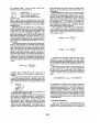
TMil statistics.
There are many Theil inequality
coefficients in use. The ones EVAL calculates are based on
relative change forecast errors, as recommended in, for
example. Leuthold (1975), to overcome sensitivity to an
additive transformation. The calculations are performed in
PROC IML according to the following:
3. Hardware. software. and data requirements
The software requirements for EVAL to run on an mM
or compatible personal computer are SAS, version 6.03 or
higher, with the following products installed: SAS/BASE,
SASiSTA~, SAS/IML, SASIETS, and SAS/ASSIST.
Extended memory is necessary; two megabytes is suggested.
SAS/AF is needed to develop an application and link it to
SAS/ASSIST; however, it is not needed to run it since the
programs are compiled.
Although EVAL was developed with a particular data base
in mind, we have tried to keep the requirements as general as
possible. The SAS data set which is to be analyzed must have
one or more variables containing "actual" values of series of
interest and one or more variables containing Mforecast· values
which are to be compared to the actual observed data.. In
addition, there must be a variable to indicate the time period
represented by each observation. It should be a numeric
variable of the form yyyyppp. with a value of 1979004, for
example. indicating the fourth period (month, quarter, etc.) of
1979 (in the future this may be generalized to handle true
SAS date variables).
n
E
t-'
(F C-AC_l)
2
+
4. Running EVAL
n
To run the EVAL Forecast Evaluation System, a user
moves the cursor on the SAS/ASSIST Primary Menu to
APPLICATIONS and presses ENTER. The next screen
provides a choice of PUBLIC (which we interpreted to mean
applications provided by SAS Institute since they currently
distn'bute some SAS/OR· examples with SAS/ASSIST) or
PRNAm (which is where we put EVAL, an application
developed at our Site). After choosing PRIVATE the user
sees a "list- of applications, of which currently EYAI... is the
only one. Placing an X by Forecast Evaluation System and
pressing ENTER places the user on another screen with
options for running the Forecast Evaluation Program, data
management, and exiting. After indicating that EVAL should
be run, a final screen is presented for specification of such
information as the data set to be analyzed, the variables to be
U2=
L
(Ft-A t ) ,
'"
n
L
t=,
(At-A t _l
) ,
These statistics compare the predictive ability of the model
generating the forecasts to the "naive" no-change model where
the forecast for the next period is this period'S actual
observation. Both VI and V2 have a lower limit of 0 which
refers to an ideal forecast, F,=A, (thUS, the smaller these
statistics, the better). For Vi the upper boundary is I, when
F,=A,.l' so that all models appear to predict at least as well as
1086
the no-change model.
The U2 statistic removes this
limitation, so that its interpretation is:
U2=O
O<U2<1
U2 = 1
U2> 1
large revision ratios may result whenever the initial forecast
itself was a very good forecast, even for revisions made in the
right direction.
Prediction Realizations. There are several steps involved in
computing prediction realization statistics, the first of which
is a -call" for an additional year of input data. In order to
eliminate seasonal bias, computations are made using the
actual values of one time period and the values of the same
relative time period of the previous year, hence the need for
To reduce the possibility of
the additional data.
misunderstanding the nature of the calculations, the input
data. including the additional year, are printed whenever
prediction realization values are requested.
Given a frequency of observation f (4 for quanerly data,
12 for monthly. and so on). a "prediction realization- is
computed as the percent change between the actual or forecast
value at time t and the actual value observed f periods (one
year) previously. That is,
perfect forecast
forecast is better than naive model
naive no-change extrapolation
forecast is worse than naive model
(Leuthold. 1975).
Note: In some cases the computed values of the Theil
statistics differ from those that would have been produced by
the SAS procedure PROe SIMNLlN. We have been unable
to duplicate by hand calculation the values that PROe
SlMNLlN prints.
Regression of actual on predicted values, y=Mx+B, as a
method of testing goodness of fil Here y is the endogenous,
actual variable A" x is the exogenous, forecast variable F" and
M and B are the slope and intercept respectively. The
solution is the result of an ordinary least squares fit of the
actual and forecasted values, with M and B estimated by
PROC REG in SASfSTAT. For perfect forecasts. F,=A,. so
that the resulting regression would have zero intercept Band
unit slope (M=1). Parameters of the regression would be
tested to see if they differed significantly from zero and one
(KosI, 1980).
Revision Ratios table and a Revision Riltio Analysis table.
These are only appropriate for examining forecast variables
from the same source, for the same actual variable, over the
same time period, when the forecasts are made at different
times. Thus more than one forecast variable name must be
Specified! The revision ratios are a measure of how well a
forecast is revised as the forecast is made at a time closer to
the period being predicted. The revision ratio between two
forecasts FA,I and FB,t' where FB,I is the forecast made later, is
calculated as the ratio of the difference between the two
forecasts (the -revision-) and the forecast error (the difference
between the original forecast and the actual observed value).
That is.
RRatio
AB,t
_
PRedR
A, t
A -A
t
t-l
At-t
A directional accuracy table, which relies upon the PR
calculations. is also available through the PR request.
However. you cannot get a directional accuracy table without
the accompanying prediction realization table. This was built
into the system to reduce possible misinterpretations of the
results.
The dire<:tional accuracy table is an interpretation of the
prediction realizations, and it uses a critical value Specified by
the user, used to set a range within which changes are
considered to be essentially zero for the purpose of directional
accuracy. Predicted and actual values that fall within the
range
F
-F
B,t
A,t
A-F
t
=100*
A, C
A forecast made 3 months ago may be a good, bad, or
indifferent revision of a forecast made six months ago, for
example.
The revision ratio analysis table summarizes the revision
ratios for the specified time period. It provides a count of the
Revision ratios which fall into each of five categories for each
of the ordered pairs of forecasts. The dasses of revision ratios
are:
Ratio = 1;
1 < Ratio < 2;
0< Ratio < 1;
Ratio <= 0;
Ratio >= 2.
Revisions falling within each class may be interpreted in
the follOwing manner (Ippolito. 1979):
A ratio equal to 1 indicates a perfect revision (equal to the
forecast error in the original time period). A ratio between 1
and 2 indicates a revision in the correct direction, but too
large. The closer the value is to 1. the better the revision. A
ratio between 0 and 1 indicates a revision in the right
direction, but too small. A ratio equal to zero means that no
revision was made, while a negative ratio indicates that the
revision was in the wrong direction. A ratio greater than or
equal to 2 means a very bad revision was made. Note that
_ Cxiticalvalue <PRedR <+ Critical Value
2
' 2
are considered as -no change.· If no critical value is specified,
a default value of 1.0 is used. The possible values in the
directional accuracy table are 0, 1, and 2, and they should be
interpreted in the following manner: a value of 0 indicates a
correct directional prediction. 1 indicates an incorrect
directional prediction, and 2 indicates a truly bad directional
prediction. Since "no change" is usually considered a direction
in forecasting analysiS, there are two steps from a correct
forecast to a horrible forecast, hence the three possible values
as explained above.
6. Anticipated enhancements
EVAL is an application under development rather than a
finished product. Several additional tests that EVAL should
perform have already been discussed with economists at
1087
USDNERS, They include Fisher Forecast Evaluation, Fisher
Fore<:ast Comparison, Wilcoxin Signed Rank. Kendall
Coefficient of Concordance, and the Mincer-Zamowitz test.
The scope of the system will thus be expanded to allow
comparisons of forecasts from different sources, as well as
evaluations of forecasts.
In order to improve performance somewhat, and to
eliminate the need for the presence ofSAS/E1S (and possibly
SAS/STA1) when running the applicatiun. we intend to
recode several EVAL modules. The menus, help screens, and
flow of the system will be altered as suggestions are made, and
time and resources allow. Output will be improved as needs
or complaints demand.
7. Conclusion
We hope that EVAL will serve as a prototype application
in SAS/ASSIST, so that others can use it as an example for
sharing applications of general interest. This framework
should be a powerful vehicle for disseminating and supporting
such programs, so that we can develop a good library of useful
procedures.
References
Granger, CW.J. and P. Newbold. "Some Comments on the
Evaluation of Economic Forecasts," Applied Economics. 5,
1973.
Ippolito, Pauline and Unda Lynn, Forecast
EYdluation System (EVAL) User's Manual. Data
Services Center Working Paper, USDA/ESCS,
March, 1979.
Kost, William E.. "Model Validation and the Net
Trade Model", Agricultural Economics
Research. Vo1.32, No.2, April, 1980.
Leuthold, Raymond M., "On the Use of Theil's
Inequality Coefficients", Arne£. J. Agr. Econ..
May 1975, p. 344·346.
Pindyck, Robert S. and Daniel L. Rubinfeld,
Econometric Models & Economic Forecasts,
McGraw-Hill, 1981.
SAS Institute Inc., SAS/AF User's Guide. Release
6.03 Edition. 1988.
SAS Institute Inc" SAS/AF Software Applications
Using Screen O)Ot101 Language Course Notes. 1989.
Theil, Henri. Economic Foreca.<:,ts and Policy, North
Holland, N.Y., 1961.
Thomson, James M., "Analysis of the Accuracy of
USDA Hog Farrowings Statistics", Am. 1. Agr.
Econ.. December, 1974.
SAS, SAS/AF, SAS/ASSIST, SASiETS. SAS/IMl> SAS/STAT
and SAS/OR are registered trademarks of SAS Institute Inc.,
Cary, NC, USA
1088
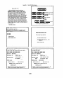
Appendix A
Selected EVAL Screens
rt)SIS'l':
Prl~ tleIllF============-lD:l~H
UelCDIII! to ElML !!!!!!!!
the Forecm. Evaluation ~leIt has been coaed as: an
applicatIon in SASlASSIST. To ICOeS5 il, MGf.Ie the cursor to
flfPLICATIOHS on the ASSIst IIIln Kelll ilM press: EHlER. The next
screen ulIl !l'lue -you 01 choIce or PUBLIC <.ippllClltiollS provided by
SAS Instibte) or PRIlMTE (applications deueloped ilt DtU' slU>.
Choose PRI1#ITE. Vau uill tun see iI. "list" of ilppllcdiou to
SElect rro~ (currentl!l ElML is the onI':! OM), Pullrl X~ Forecast
Euailliltion S!JSlM and prm lItTER. ~ou ulll hi! given iIIOHer list
of Clplions IIiIlch include an!! illY ediU", you llDUid like to do Dr
ruml", th! Forecast Euilillitlon pr0!ll'ifl, Put in Xh!f the approprh.le
option aM press EKIER. Once In the IE'III for MI., !IDlI ulll IIIIUe
!PUr" cursor II'OlU'III tile screen to fill in such inl'ol"'lliltlon is till!
aata set you IIIsh to illai!!ze, tile uarlil.hh ultla conblns tile actual
values: fIr the series of interest, the Virlable or uariules: ubich
conhin farecans !IN uollld lU:e to Co"pll'e t.o the ,dual "dues. w
the tYPe's of ilndyses !jIIU uish to perfort\. Press PFl at illl9 paint al
uIIicll you 1'11!811 help.
TWJe of Application:
Tab to
iI1I
option ilnd press DlTER
to !OVled.
Press EIITER to oontiu.
I
1ST: AppUuUon Seleclio .-======-===18:
•
l1~n
Select the appl!callon
!:IOU UilTll
to
I'IIfI.
Place ill19 Wricler in the field neid to tie application descripUon.
Pres5 DfTEII to ~ the selected ippllcallon: use ;om to return.
plication $elecUo,o=--..;,;,..------------;
Place
In
Xnekt to !jOur selection:
Run Foretisl Euilual10n PI'<Igl'1lI
_
Dib.llaNsenenl (select.. edil. etc., if not
dread9 dore)
Rrlurn to Preulous Hew
Auarlable of actual values is required. DfTER to Klke a selecllon.
Tab ind press 1ltTFJl1o select.
fCClUE data set: _A.PRICIS
fCIUE dab. set: AGMIURltES
MTE Indicalor: TII!E
DIllE IndiCillor: TIllE
~ol'dab.:
INITIAL TII!E PERIOD: 19&1981
InITIAl.. TitlE PERIOD:
ACtIW. value Worlable:
tcML willi! IIIl'lable:
BESCP\JS
LAST TItlE IIRIOD:
FORECASt wrlilhle&:
DISPiJIY Input data: I«l
IEStPUJ] BESCPlIlr.
DISM Input ull: VIS
HIL sliUdics: III
IDilIESSII»t of actllloi In predicted. wlues: III
THEIL shU sUes: YES
REGRESSION af aclUilI an predlcted. wdues.! YES
RlUISIat ratios! 110
HUIS[lxt raUGS: YES
PiEIlICTIIJI - reallntloTl lind directlollill iCcur~ $bUstles: ItO
CriUCil w,lue (for dlrecUol'lll accur'iC!I COltpub.tlons): 1.8
PREDICTION - reaUuUcm and diredlonal iCCur~ shlisllcs:: YES
Critical value <for directional ~ CDltpub.llons): 1.8
1089
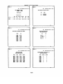
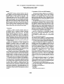
Appendix B. Selected EVAI.. Output
;Mm---====-=======I':I~
jOOII_==============I':11M
ColNniI-)
18:89~.
W
ntEIL:
"""
SAS
llarck 15. 1999
~ - BESCPlIS
IXIIGOOE - JEStIUI3
18:89 ThuNday. llarch 15, 1999
MIL stATISTICS FOIl BEStPIlS, BI:SCPUI3
SIIILIH ProcedUl't!
sm!
tw.IIE
ShtistIcs of fit
Ut:
UZ •
B.3a1i'28l595
'.SS1!898618
lleiln
~
Uirlable
Im>,
,,,"
B&!CIIlS
4.31!lI
'.8m
""nAl><
"""
""" (0,
Yo Error
117.8168
IllS
,,,"
Z.I3G4!I 151.1593
.,"
Im>,
Z.U
1':1""
,oorPllT================1":1,,"
"","",,->
"""'"
SfIS
>
SiIS
18: 89 Ihlll'Sda!l. llarci 15, 1998 18
RIlIISIlii l1IIIIOS ro! 8ESCPUS BlICPUI3 8ESCPUI6
RWIIIO" RAllO
18: M Tlwr>daY. Harch 15, 1998 11
AIIAL~II
!ABLE
BESCPUS BESCPUI3 ECPU!6
PERIOD
lUZ
1981111
ISIIIII£
IliUm
13.6364
1.313'
1.3899
RaUl = 1
l(iaUo(Z
B(RaUo(l
19811114
19BZ1111t
8.8IIB8
hth
-I.M
ISlzseZ
IlIZ81!3
19_
8.SSZ3
8.6151
B.8475
COLI
(=
COLI
B
Ratio); Z
b.===========~:ZOO~~,d
18: 1SA11
CoMml_>
SiIS
,oor1lJI================lj':1IA11
ColNniI - )
18:89 Iktrsday. Hirch 15, 1998 13
$AS
PBEbltTIlii RmLlZOlTIlii
8ESCPIIS 8ESCPUI3 BEScPUI'
PERIOD
ACTIML
1!J911ll1
5.9439'1
3.58489
lSIllII£
lSIl883
lSIl884
l!82881
1!18Z88Z
1982883
198Z81!4
2.91£85
l.Ii47Z7
-1..13
-1.32415
3.41894
Z.48311
IBlDltTl
18:89 Tfwrsday. llarch 15, 1999 14
IIBltTUM ACC\JRAt'I CRITICAL tw.IIE II 1.1
BEScPlIS BESCIIJI3 BESCPUI'
IBlDltT2
PERIOD
8.~U
5.73443
-Z.81564
4.41613
-1.521!3
",.68444
1981881
1981lez
1981883
1981884
198Z8I!1
198Z8I!Z
j98Z8l!3
198Z8I!4
1.15881
-1.89584
-1.5Z1!3
..a.1m1
-1.56394
1.16!lS2
2.166'4
-Z.943i8
1.96115
1.48514
1090
IlEDICTl
lR!Dlcrz